Embed Size (px)
Citation preview
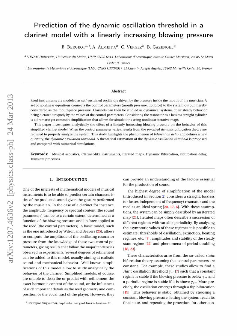
Prediction of the dynamic oscillation threshold in aclarinet model with a linearly increasing blowing pressure
B. BERGEOTa,∗, A. ALMEIDAa , C. VERGEZb , B. GAZENGELa
a LUNAM Université, Université du Maine, UMR CNRS 6613, Laboratoire d’Acoustique, Avenue Olivier Messiaen, 72085 Le Mans
Cedex 9, Franceb Laboratoire de Mécanique et Acoustique (LMA, CNRS UPR7051), 31 Chemin Joseph Aiguier, 13402 Marseille Cedex 20, France
Abstract
Reed instruments are modeled as self-sustained oscillators driven by the pressure inside the mouth of the musician. A
set of nonlinear equations connects the control parameters (mouth pressure, lip force) to the system output, hereby
considered as the mouthpiece pressure. Clarinets can then be studied as dynamical systems, their steady behavior
being dictated uniquely by the values of the control parameters. Considering the resonator as a lossless straight cylinder
is a dramatic yet common simplification that allows for simulations using nonlinear iterative maps.
This paper investigates analytically the effect of a linearly increasing blowing pressure on the behavior of this
simplified clarinet model. When the control parameter varies, results from the so-called dynamic bifurcation theory are
required to properly analyze the system. This study highlights the phenomenon of bifurcation delay and defines a new
quantity, the dynamic oscillation threshold. A theoretical estimation of the dynamic oscillation threshold is proposed
and compared with numerical simulations.
Keywords: Musical acoustics, Clarinet-like instruments, Iterated maps, Dynamic Bifurcation, Bifurcation delay,
Transient processes.
1. INTRODUCTION
One of the interests of mathematical models of musical
instruments is to be able to predict certain characteris-
tics of the produced sound given the gesture performed
by the musician. In the case of a clarinet for instance,
the amplitude, frequency or spectral content (the sound
parameters) can be to a certain extent, determined as a
function of the blowing pressure and lip force applied to
the reed (the control parameters). A basic model, such
as the one introduced by Wilson and Beavers [25], allows
to compute the amplitude of the oscillating resonator
pressure from the knowledge of these two control pa-
rameters, giving results that follow the major tendencies
observed in experiments. Several degrees of refinement
can be added to this model, usually aiming at realistic
sound and mechanical behavior. Well known simpli-
fications of this model allow to study analytically the
behavior of the clarinet. Simplified models, of course,
are unable to describe or predict with refinement the
exact harmonic content of the sound, or the influences
of such important details as the reed geometry and com-
position or the vocal tract of the player. However, they
∗Corresponding author, [email protected]
can provide an understanding of the factors essential
for the production of sound.
The highest degree of simplification of the model
(introduced in Section 2) considers a straight, lossless
(or losses independent of frequency) resonator and the
reed as an ideal spring [20, 17, 6]. With these assump-
tions, the system can be simply described by an iterated
map [21]. Iterated maps often describe a succession of
different regimes with variable periodicity. By analyzing
the asymptotic values of these regimes it is possible to
estimate: thresholds of oscillation, extinction, beating
regimes, etc. [7], amplitudes and stability of the steady
state regime [22] and phenomena of period doubling
[18, 23].
These characteristics arise from the so-called static
bifurcation theory assuming that control parameters are
constant. For example, these studies allow to find a
static oscillation threshold γst [7] such that a constant
regime is stable if the blowing pressure is below γst and
a periodic regime is stable if it is above γst . More pre-
cisely, the oscillation emerges through a flip bifurcation
[19]. This behavior is static, obtained by choosing a
constant blowing pressure, letting the system reach its
final state, and repeating the procedure for other con-
arX
iv:1
207.
4636
v2 [
phys
ics.
clas
s-ph
] 2
4 M
ar 2
013

2 B. Bergeot et al.
stant blowing pressures. Therefore, most studies using
iterated map approach are restricted to a steady state
analysis of the oscillation, even if transients are studied.
They focus on the asymptotic amplitude regardless of
the history of the system.
During a note attack transient the musician varies
the pressure in her/his mouth before reaching a quasi-
constant value. During this transient the blowing pres-
sure cannot be regarded as constant. In a mathematical
point of view increasing the control parameter (here the
blowing pressure) makes the system non-autonomous
and results from static bifurcation theory are not suf-
ficient to describe its evolution. Indeed, it is known
that, when the control parameter varies, the bifurcation
point – i.e. the value of the blowing pressure where
the system begins to oscillate – can be considerably de-
layed [16, 2, 13]. Indeed, the bifurcation point is shifted
from γst to a larger value γd t called dynamic oscillation
threshold. This phenomenon called bifurcation delay
is not predicted by the static theory. Therefore, when
the control parameter varies, results from the so-called
dynamic bifurcation theory are required to properly an-
alyze the system.
The purpose of this paper is to use results from dy-
namic bifurcation theory to describe analytically a sim-
plified clarinet model taking into account a blowing
pressure that varies linearly with time. In particular we
propose a theoretical estimation of the dynamic oscilla-
tion threshold.
Section 2 introduces the simplified mathematical
model of a clarinet and the iterated map method used to
estimate the existence of the oscillations inside the bore
of the clarinet. Some results related to the steady state
are presented in this section. Section 3 is devoted to the
study of the dynamic system that takes into account a
linearly increasing blowing pressure. The phenomenon
of bifurcation delay is demonstrated using numerical
simulations. A theoretical estimation of the dynamic os-
cillation threshold is also presented and compared with
numerical simulations. In Section 4 the limits of this
approach are discussed. It is shown, when the model
is simulated, that the precision (the number of decimal
digits used by the computer) has a dramatic influence
on the bifurcation delay. The influence of the speed at
which the blowing pressure is swept is also discussed.
2. STATE OF THE ART
2.1 Elementary model
The model of the clarinet system used in this article fol-
lows an extreme simplification of the instrument, which
can be found in other theoretical works [20, 6].
y(t)
−H
0 U(t) Ur(t)Uin(t)
P (t)
Mouthpiece
Reed
Lip
Mouth
Pm
Reed channel
Figure 1: Schematic diagram of a single-reed mouthpiece.Presentation of variables, control parameters and choice ofaxis orientation. U is the flow created by the pressure imbal-ance Pm −P between the mouth and the bore, Ur is the flowcreated by the motion of the reed, Ui n is the flow entering theinstrument, y represents the position of the tip of the reed andH is the opening of the reed channel at rest.
This basic model separates the instrument into two
functional elements. One of these is the bore, or res-
onator, a linear element where the pressure waves prop-
agate without losses. The other is the reed-mouthpiece
system, which is considered as a valve controlled by the
pressure difference between the mouth and the mouth-
piece. It is often called the generator and is the only
nonlinear part of the instrument. A table of notation is
provided in Appendix A.
2.1.1 The reed-mouthpiece system
The reed-mouthpiece system is depicted in Fig. 1. The
reed is assumed to behave as an ideal spring charac-
terized by its static stiffness per unit area Ks . So, its
response y to the pressure difference ∆P = Pm −P is
linear and is given by:
y =−∆P
Ks. (1)
From (1) we can define the static closing pressure
PM which corresponds to the lowest pressure that com-
pletely closes the reed channel (y =−H):
PM = Ks H . (2)
The reed model also considers that the flow created
by the motion of the reed Ur is equal to zero, so that
the only flow entering the instrument is created by the
pressure imbalance between the mouth and the bore:
Ui n =U . (3)
The non-linearity of the reed-mouthpiece system is
introduced by the Bernoulli equation which relates the
flow U to the acoustic pressure P [15, 14]. This relation
is the nonlinear characteristics of the exciter, given by:
Prediction of the dynamic oscillation threshold in a clarinet model with a linearly increasing blowing pressure 3
U =
UA
(1− ∆P
PM
)√|∆P |PM
sgn(∆P )
if ∆P < PM ; (4a)
0
if ∆P > PM . (4b)
The flow UA is calculated using the Bernoulli theo-
rem:
UA = S
√2PM
ρ, (5)
where S is the opening cross section of the reed channel
at rest and ρ the density of the air.
Introducing the dimensionless variables and control
parameters [6]:
∆p =∆P/PM
p = P/PM
u = Zc U /PM
γ = Pm/PM
ζ = Zc UA/PM .
(6)
Zc = ρc/Sr es is the characteristic impedance of the cylin-
drical resonator of cross-section Sr es (c is the sound
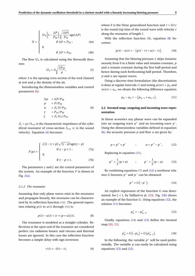
velocity). Equation (4) becomes:
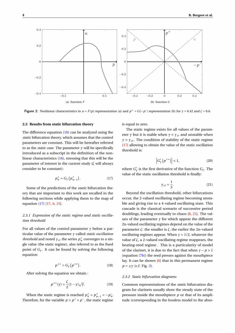
F (p) =
ζ(1−γ+p
)√|γ−p|sgn(γ−p)
if γ−p < 1 ; (7a)
0
if γ−p > 1. (7b)
The parameters γ and ζ are the control parameters of
the system. An example of the function F is shown in
Fig. 2(a).
2.1.2 The resonator
Assuming that only plane waves exist in the resonator
and propagate linearly, the resonator can be character-
ized by its reflection function r (t). The general expres-
sion relating p(t ) to u(t ) through r (t ) is:
p(t )−u(t ) = [r ∗ (p +u)](t ). (8)
The resonator is modeled as a straight cylinder. Re-
flections at the open end of the resonator are considered
perfect (no radiation losses) and viscous and thermal
losses are ignored. In this case the reflection function
becomes a simple delay with sign inversion:
r (t ) =−δ(t −τ), (9)
where δ is the Dirac generalized function and τ= 2l/c
is the round trip time of the sound wave with velocity c
along the resonator of length l .
With the reflection function (9), equation (8) be-
comes:
p(t )−u(t ) =−[p(t −τ)+u(t −τ)
]. (10)
Assuming that the blowing pressure γ skips instanta-
neously from 0 to a finite value and remains constant, p
and u remain constant during the first half-period and
hence during each forthcoming half-period. Therefore,
p and u are square waves.
Using a discrete time formulation (the discretization
is done at regular intervals τ) and noting p(nτ) = pn and
u(nτ) = un , we obtain the following difference equation:
pn −un =−(pn−1 +un−1
). (11)
2.2 Iterated map: outgoing and incoming wave repre-sentation
In linear acoustics any planar wave can be expanded
into an outgoing wave p+ and an incoming wave p−.
Using the dimensionless variables defined in equation
(6), the acoustic pressure p and flow u are given by:
p = p++p− ; u = p+−p−, (12)
Replacing in equation (11),
p+ = 1
2(p +u) ; p− = 1
2(p −u). (13)
By combining equations (7) and (12) a nonlinear rela-
tion G between p+ and p− can be obtained:
p+ =G(−p−)
. (14)
An explicit expression of the function G was deter-
mined, for ζ< 1, by Taillard et al. [23]. Fig. 2(b) shows
an example of the function G . Using equations (12), the
relation (11) becomes:
p−n =−p+
n−1. (15)
Finally, equations (14) and (15) define the iterated
map [20, 21]:
p+n =G
(−p−n
)=G(p+
n−1
). (16)
In the following, the variable p+ will be used prefer-
entially. The variable p can easily be calculated using
equations (15) and (12).
4 B. Bergeot et al.
−0.5 0.5−0.4
−0.2
0
0.2
0.4u
p
(a) function F
−0.4 −0.2 0 0.2 0.4
−0.4
−0.2
0
0.2
0.4up
−p−
p+
(b) function G
Figure 2: Nonlinear characteristics in u = F (p) representation (a) and p+ =G(−p-) representation (b) for γ= 0.42 and ζ= 0.6.
2.3 Results from static bifurcation theory
The difference equation (16) can be analyzed using the
static bifurcation theory, which assumes that the control
parameters are constant. This will be hereafter referred
to as the static case. The parameter γ will be specifically
introduced as a subscript in the definition of the non-
linear characteristics (16), stressing that this will be the
parameter of interest in the current study (ζ will always
consider to be constant):
p+n =Gγ
(p+
n−1
). (17)
Some of the predictions of the static bifurcation the-
ory that are important to this work are recalled in the
following sections while applying them to the map of
equation (17) [17, 6, 23].
2.3.1 Expression of the static regime and static oscilla-
tion threshold
For all values of the control parameter γ below a par-
ticular value of the parameter γ called static oscillation
threshold and noted γst the series p+n converges to a sin-
gle value (the static regime), also referred to as the fixed
point of Gγ. It can be found by solving the following
equation:
p+∗ =Gγ
(p+∗)
. (18)
After solving the equation we obtain :
p+∗(γ) = ζ
2(1−γ)
pγ. (19)
When the static regime is reached p+n = p+
n−1 =−p−n .
Therefore, for the variable p = p++p−, the static regime
is equal to zero.
The static regime exists for all values of the param-
eter γ but it is stable when γ< γst and unstable when
γ > γst . The condition of stability of the static regime
[17] allowing to obtain the value of the static oscillation
threshold is: ∣∣∣G ′γ
(p+∗)∣∣∣< 1, (20)
where G ′γ is the first derivative of the function Gγ. The
value of the static oscillation threshold is finally:
γst = 1
3. (21)
Beyond the oscillation threshold, other bifurcations
occur, the 2-valued oscillating regime becoming unsta-
ble and giving rise to a 4-valued oscillating state. This
cascade is the classical scenario of successive period
doublings, leading eventually to chaos [8, 23]. The val-
ues of the parameter γ for which appear the different
2n-valued oscillating regimes depend on the value of the
parameter ζ: the smaller is ζ, the earlier the 2n-valued
oscillating regimes appear. When γ= 1/2, whatever the
value of ζ, a 2-valued oscillating regime reappears, the
beating-reed regime . This is a particularity of model
of the clarinet, it is due to the fact that when γ−p > 1
(equation (7b)) the reed presses against the mouthpiece
lay. It can be shown [6] that in this permanent regime
p =±γ (c.f. Fig. 3).
2.3.2 Static bifurcation diagrams
Common representations of the static bifurcation dia-
gram for clarinets usually show the steady state of the
pressure inside the mouthpiece p or that of its ampli-
tude (corresponding in the lossless model to the abso-
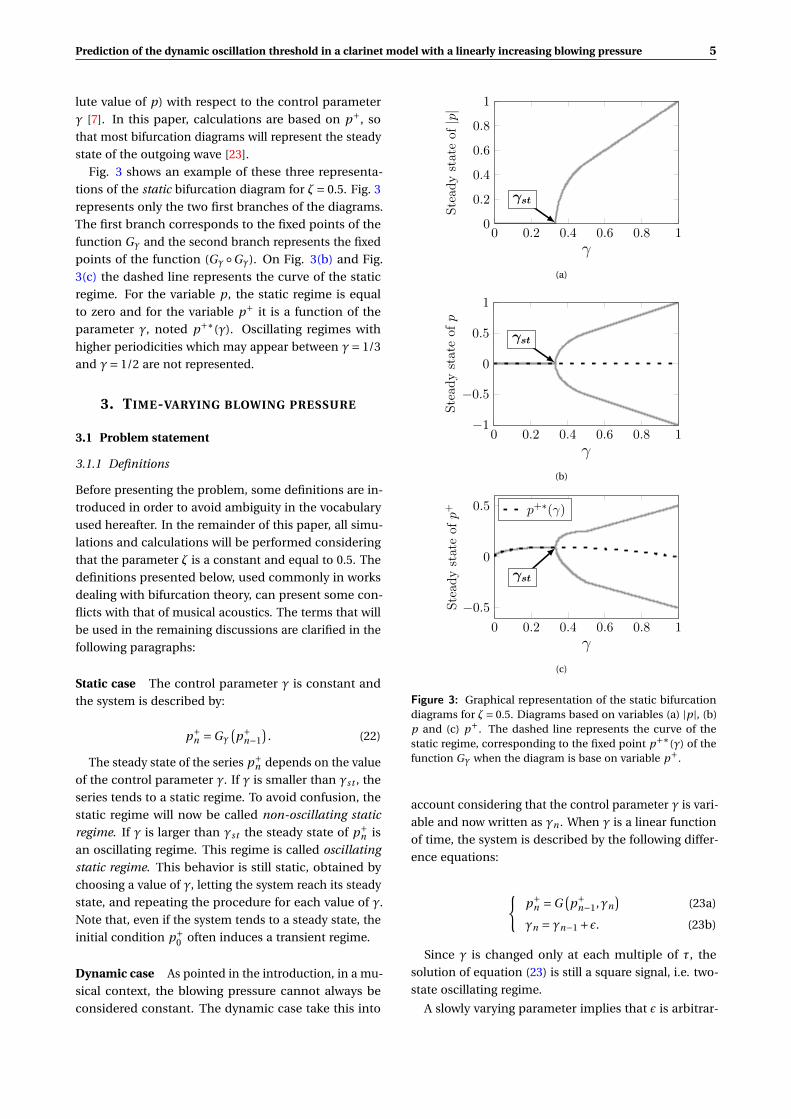
Prediction of the dynamic oscillation threshold in a clarinet model with a linearly increasing blowing pressure 5
lute value of p) with respect to the control parameter
γ [7]. In this paper, calculations are based on p+, so
that most bifurcation diagrams will represent the steady
state of the outgoing wave [23].
Fig. 3 shows an example of these three representa-
tions of the static bifurcation diagram for ζ= 0.5. Fig. 3
represents only the two first branches of the diagrams.
The first branch corresponds to the fixed points of the
function Gγ and the second branch represents the fixed
points of the function (Gγ ◦Gγ). On Fig. 3(b) and Fig.
3(c) the dashed line represents the curve of the static
regime. For the variable p, the static regime is equal
to zero and for the variable p+ it is a function of the
parameter γ, noted p+∗(γ). Oscillating regimes with
higher periodicities which may appear between γ= 1/3
and γ= 1/2 are not represented.
3. TIME-VARYING BLOWING PRESSURE
3.1 Problem statement
3.1.1 Definitions
Before presenting the problem, some definitions are in-
troduced in order to avoid ambiguity in the vocabulary
used hereafter. In the remainder of this paper, all simu-
lations and calculations will be performed considering
that the parameter ζ is a constant and equal to 0.5. The
definitions presented below, used commonly in works
dealing with bifurcation theory, can present some con-
flicts with that of musical acoustics. The terms that will
be used in the remaining discussions are clarified in the
following paragraphs:
Static case The control parameter γ is constant and
the system is described by:
p+n =Gγ
(p+
n−1
). (22)
The steady state of the series p+n depends on the value
of the control parameter γ. If γ is smaller than γst , the
series tends to a static regime. To avoid confusion, the
static regime will now be called non-oscillating static
regime. If γ is larger than γst the steady state of p+n is
an oscillating regime. This regime is called oscillating
static regime. This behavior is still static, obtained by
choosing a value of γ, letting the system reach its steady
state, and repeating the procedure for each value of γ.
Note that, even if the system tends to a steady state, the
initial condition p+0 often induces a transient regime.
Dynamic case As pointed in the introduction, in a mu-
sical context, the blowing pressure cannot always be
considered constant. The dynamic case take this into
γst
0 0.2 0.4 0.6 0.8 10
0.2
0.4
0.6
0.8
1
γ
Stea
dyst
ate
of|p|
(a)
γst
0 0.2 0.4 0.6 0.8 1−1
−0.5
0
0.5
1
γSt
eady
stat
eof
p
(b)
γst
0 0.2 0.4 0.6 0.8 1
−0.5
0
0.5
γ
Stea
dyst
ate
ofp+ p+∗(γ)
(c)
Figure 3: Graphical representation of the static bifurcationdiagrams for ζ= 0.5. Diagrams based on variables (a) |p|, (b)p and (c) p+. The dashed line represents the curve of thestatic regime, corresponding to the fixed point p+∗(γ) of thefunction Gγ when the diagram is base on variable p+.
account considering that the control parameter γ is vari-
able and now written as γn . When γ is a linear function
of time, the system is described by the following differ-
ence equations:
{p+
n =G(p+
n−1,γn)
(23a)
γn = γn−1 +ε. (23b)
Since γ is changed only at each multiple of τ, the
solution of equation (23) is still a square signal, i.e. two-
state oscillating regime.
A slowly varying parameter implies that ε is arbitrar-

6 B. Bergeot et al.
0 100 200 300 400 500 600 700 800
−0.4
−0.2
0
0.2
0.4
0.6
0.8
1
n
p+ n
p+nγn
(a)
Non-oscillating dynamic regime
Transient oscillatingdynamic regime
Final oscillatingdynamic regime
0 50 100 150 200 250 3000.04
0.06
0.08
0.1
0.12
0.14
n
p+ n
(b)
Figure 4: Numerical simulation performed on the system (23). (a) complete orbit of the series and (b) zoom near the non-oscillation dynamic regime. ζ= 0.5, ε= 10−3, γ0 = 0.2 and p+
0 =G(0,γ0).
ily small (ε¿ 1). The hypothesis of an arbitrarily small
ε could be questioned in the context of the playing of
a musical instrument. However, this hypothesis is re-
quired in order to use the framework of dynamic bifur-
cation theory (see forthcoming sections).
An example of a numerical simulation performed on
the system (23) is shown in Fig. 4 for ζ = 0.5, ε = 10−3
and an initial condition γ0 = 0.2. The initial value of the
outgoing wave is p+0 =G(−p−
0 = 0,γ0). Indeed, for n = 0
the incoming wave p− is clearly zero, otherwise sound
would have traveled back and forth with an infinite ve-
locity.
The series p+n first shows a short oscillating transient,
which will be called transient oscillating dynamic regime.
This oscillation decays into a non-oscillating dynamic
regime. Beyond a certain threshold, a new oscillation
grows, giving rise to the final oscillating dynamic regime.
This paper will focus on the transition (i.e. the bi-
furcation) from the non-oscillating dynamic regime to
the final oscillating dynamic regime. The value of the
parameter γ for which the bifurcation occurs is called
dynamic oscillation threshold, noted γd t .
3.1.2 Bifurcation delay
Bifurcation delay occurs in nonlinear-systems with time
varying control parameters. Fruchard and Schäfke [13]
published an overview of the problem of bifurcation
delay.
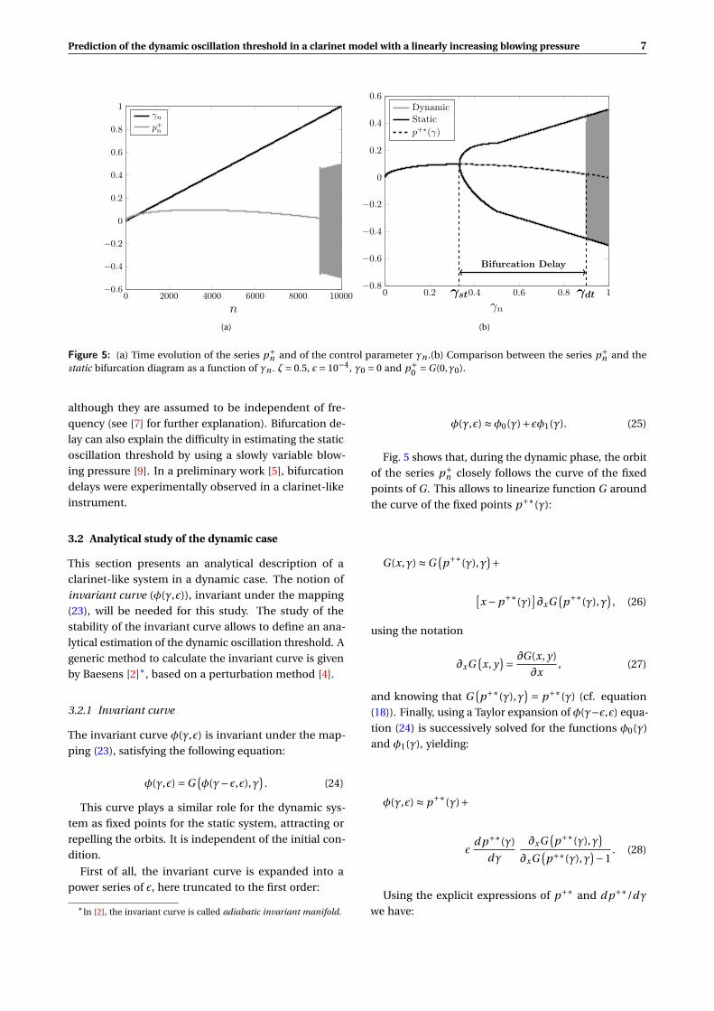
In fig. 5, the system (23) was simulated numerically,
showing the time evolution of the series p+n and of the
control parameter γn (cf. Fig. 5(a)). To better under-
stand the consequence of a time-varying parameter, the
orbit of the series p+n is plotted as a function of the pa-
rameter γn – in this case the evolution of the system can
be interpreted as a dynamic bifurcation diagram. This is
compared to the static bifurcation diagram in Fig. 5(b).
We can observe that the static and the dynamic bifur-
cation diagrams coincide far from the static oscillation
threshold γst . However, in the dynamic case, we can see
that the orbit continues to follow closely the branch of
the fixed point of function G throughout a remarkable
extent of its unstable range, i.e. after γst : the bifurca-
tion point is shifted from the static oscillation threshold
γst to the dynamic oscillation threshold γd t . The term
bifurcation delay is used to state the fact that the static
oscillation threshold γst is smaller than the dynamic
oscillation threshold γd t .
Non-standard analysis has been used in the past to
study the phenomenon of bifurcation delay [11, 12], ex-
plaing that one of the causes of the bifurcation delay is
the exponential proximity between the orbit of the se-
ries p+n and the curve of the the fixed point of G . Other
studies of bifurcation delay using standard mathemat-
ical tools – mathematics [2, 3] or physics publications
[16, 24] – explain bifurcation delay as an accumulation
of stability during the range of γ for which the fixed
point of G is stable (i.e. 0 < γn < γst ). The dynamic os-
cillation threshold therefore appears as the value of the
parameter γ at which the stability previously accumu-
lated is compensated.
In musical acoustics literature some papers present
results showing the phenomenon of bifurcation delay
without never making a connection to the concept of
dynamic bifurcation. For example this phenomenon is
observed in simulations of clarinet-like systems using
a slightly more sophisticated clarinet model (Raman’s
model) [1]. Raman’s model takes losses into account
Prediction of the dynamic oscillation threshold in a clarinet model with a linearly increasing blowing pressure 7
0 2000 4000 6000 8000 10000−0.6
−0.4
−0.2
0
0.2
0.4
0.6
0.8
1
n
γnp+n
(a)
0 0.2 γst0.4 0.6 0.8 γdt 1−0.8
−0.6
−0.4
−0.2
0
0.2
0.4
0.6
Bifurcation Delay
γn
DynamicStaticp+∗(γ)
(b)
Figure 5: (a) Time evolution of the series p+n and of the control parameter γn .(b) Comparison between the series p+
n and thestatic bifurcation diagram as a function of γn . ζ= 0.5, ε= 10−4, γ0 = 0 and p+
0 =G(0,γ0).
although they are assumed to be independent of fre-
quency (see [7] for further explanation). Bifurcation de-
lay can also explain the difficulty in estimating the static
oscillation threshold by using a slowly variable blow-
ing pressure [9]. In a preliminary work [5], bifurcation
delays were experimentally observed in a clarinet-like
instrument.
3.2 Analytical study of the dynamic case
This section presents an analytical description of a
clarinet-like system in a dynamic case. The notion of
invariant curve (φ(γ,ε)), invariant under the mapping
(23), will be needed for this study. The study of the
stability of the invariant curve allows to define an ana-
lytical estimation of the dynamic oscillation threshold. A
generic method to calculate the invariant curve is given
by Baesens [2]∗, based on a perturbation method [4].
3.2.1 Invariant curve
The invariant curve φ(γ,ε) is invariant under the map-
ping (23), satisfying the following equation:
φ(γ,ε) =G(φ(γ−ε,ε),γ
). (24)
This curve plays a similar role for the dynamic sys-
tem as fixed points for the static system, attracting or
repelling the orbits. It is independent of the initial con-
dition.
First of all, the invariant curve is expanded into a
power series of ε, here truncated to the first order:
∗In [2], the invariant curve is called adiabatic invariant manifold.
φ(γ,ε) ≈φ0(γ)+εφ1(γ). (25)
Fig. 5 shows that, during the dynamic phase, the orbit
of the series p+n closely follows the curve of the fixed
points of G . This allows to linearize function G around
the curve of the fixed points p+∗(γ):
G(x,γ) ≈G(p+∗(γ),γ
)+[x −p+∗(γ)
]∂xG
(p+∗(γ),γ
), (26)
using the notation
∂xG(x, y
)= ∂G(x, y)
∂x, (27)
and knowing that G(p+∗(γ),γ
) = p+∗(γ) (cf. equation
(18)). Finally, using a Taylor expansion of φ(γ−ε,ε) equa-
tion (24) is successively solved for the functions φ0(γ)
and φ1(γ), yielding:
φ(γ,ε) ≈ p+∗(γ)+
εd p+∗(γ)
dγ
∂xG(p+∗(γ),γ
)∂xG
(p+∗(γ),γ
)−1. (28)
Using the explicit expressions of p+∗ and d p+∗/dγ
we have:
8 B. Bergeot et al.
0 5 · 10−2 0.1 0.15 0.2 0.25 0.3
0.4
0.6
0.8
1
©
γ0
γth dt
(a) ε= 10−2
0 5 · 10−2 0.1 0.15 0.2 0.25 0.3
0.4
0.6
0.8
1
©
γ0
γth dt
(b) ε= 10−3
0 5 · 10−2 0.1 0.15 0.2 0.25 0.3
0.4
0.6
0.8
1
©
γ0
γth dt
(c) ε= 10−4
0 5 · 10−2 0.1 0.15 0.2 0.25 0.3
0.4
0.6
0.8
1
γ0
γth dt
ε = 10−2
ε = 10−3
ε = 10−4
(d)
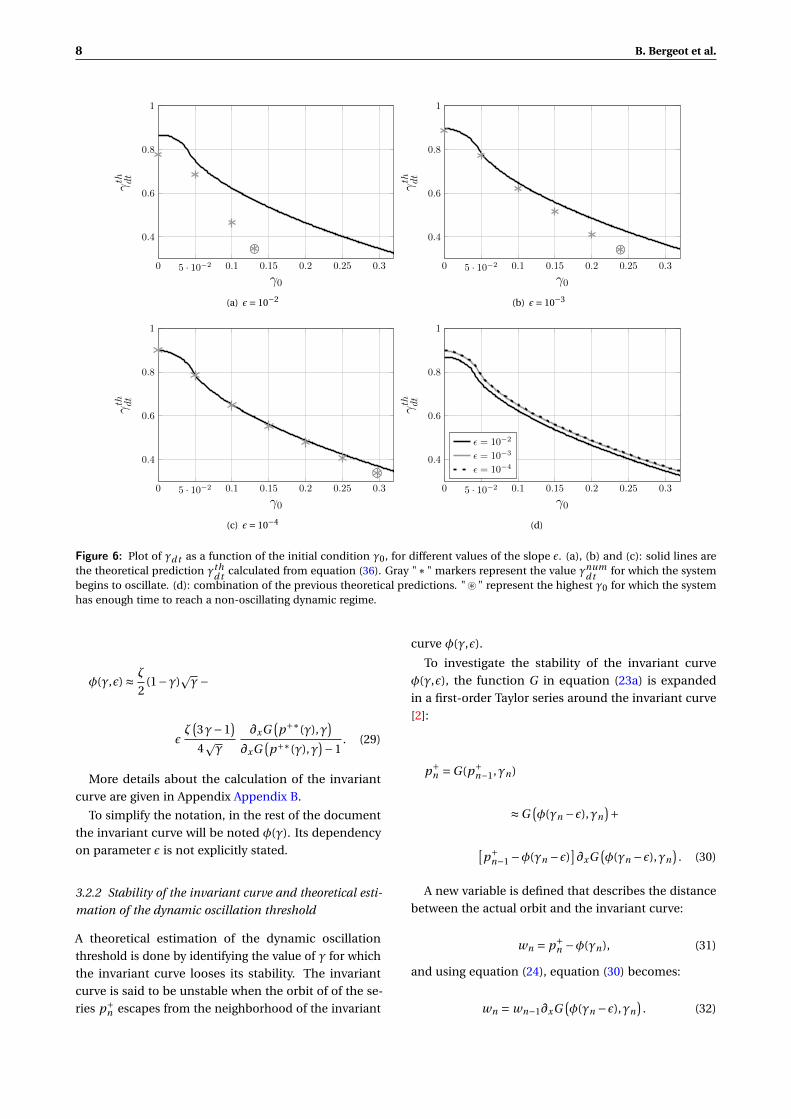
Figure 6: Plot of γd t as a function of the initial condition γ0, for different values of the slope ε. (a), (b) and (c): solid lines arethe theoretical prediction γth
d t calculated from equation (36). Gray "∗" markers represent the value γnumd t for which the system
begins to oscillate. (d): combination of the previous theoretical predictions. "~" represent the highest γ0 for which the systemhas enough time to reach a non-oscillating dynamic regime.
φ(γ,ε) ≈ ζ
2(1−γ)
pγ−
εζ(3γ−1
)4pγ
∂xG(p+∗(γ),γ
)∂xG
(p+∗(γ),γ
)−1. (29)
More details about the calculation of the invariant
curve are given in Appendix Appendix B.
To simplify the notation, in the rest of the document
the invariant curve will be noted φ(γ). Its dependency
on parameter ε is not explicitly stated.
3.2.2 Stability of the invariant curve and theoretical esti-
mation of the dynamic oscillation threshold
A theoretical estimation of the dynamic oscillation
threshold is done by identifying the value of γ for which
the invariant curve looses its stability. The invariant
curve is said to be unstable when the orbit of of the se-
ries p+n escapes from the neighborhood of the invariant
curve φ(γ,ε).
To investigate the stability of the invariant curve
φ(γ,ε), the function G in equation (23a) is expanded
in a first-order Taylor series around the invariant curve
[2]:
p+n =G(p+
n−1,γn)
≈G(φ(γn −ε),γn
)+[p+
n−1 −φ(γn −ε)]∂xG
(φ(γn −ε),γn
). (30)
A new variable is defined that describes the distance
between the actual orbit and the invariant curve:
wn = p+n −φ(γn), (31)
and using equation (24), equation (30) becomes:
wn = wn−1∂xG(φ(γn −ε),γn
). (32)
Prediction of the dynamic oscillation threshold in a clarinet model with a linearly increasing blowing pressure 9
The solution of equation (32) is formally:
wn = w0
n∏i=1
∂xG(φ(γi −ε),γi
), (33)
for n ≥ 1 and where w0 is the initial value of wn . The
absolute value of wn can be written as follow:
|wn | =
|w0|exp
(n∑
i=1ln
∣∣∂xG(φ(γi −ε),γi
)∣∣) . (34)
Finally, using Euler’s approximation the sum is re-
placed by an integral:
|wn | ≈
|w0|exp
(∫ γn+ε
γ0+εln
∣∣∂xG(φ(γ′−ε),γ′
)∣∣ dγ′
ε
). (35)
Equation (35) shows that the variable p+ starts to
diverge from the invariant curve φ(γ,ε) when the argu-
ment of the exponential function changes from negative
to positive. Therefore, the analytical estimation of the
dynamic oscillation threshold γthd t is defined by:
∫ γthd t+ε
γ0+εln
∣∣∂xG(φ(γ′−ε),γ′
)∣∣dγ′ = 0, (36)
where γ0 is the initial value of γ. This result can be de-
duced from [2] (equation (2.18)), it may also be obtained
in the framework of non-standard analysis [10].
The theoretical estimation γthd t of the dynamic oscilla-
tion threshold depends on the initial condition γ0 and
on the increase rate ε, it is therefore written γthd t (γ0,ε).
A numerical solution γthd t (γ0,ε) of the implicit equa-
tion (36) is plotted in Fig. 6 as a function of the initial
condition γ0 and for ε= 10−2, 10−3 and 10−4. γthd t can be
much larger than static oscillation threshold γst = 1/3
for small initial conditions γ0. When the initial condi-
tion value γ0 increases, γthd t approaches the static thresh-
old. Fig. 6(d) shows that the bifurcation delay seems
to be independent of the increase rate ε if this value is
sufficiently small (typically ≤ 10−3).
Equation (36) states that when γ= γthd t we have |wn | ≈
|w0|, providing a good estimation of the dynamic oscil-
lation threshold γd t if |w0| is sufficiently small, i.e. if p+0
is sufficiently close to φ(γ0). γ0 = 0 can be problematic
since φ(0,ε) =−∞, but a single iteration is sufficient to
bring the orbit to a neighborhood of the invariant curve.
Therefore, we make the assumption that
γthd t (0,ε) ≈ γth
d t (ε,ε). (37)
0.3 0.35 0.4 0.45 0.5−0.4
−0.3
−0.2
−0.1
0
0.1
0.2
0.3
γn
p+ n
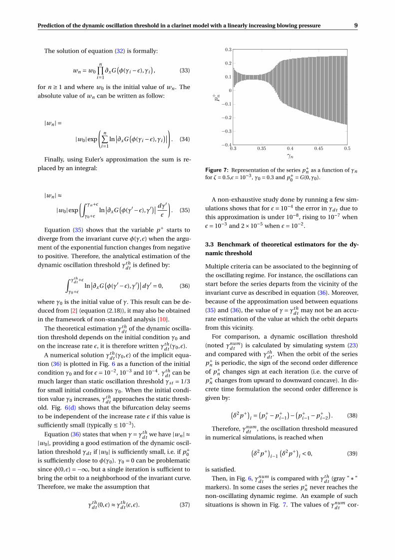
Figure 7: Representation of the series p+n as a function of γn
for ζ= 0.5,ε= 10−3, γ0 = 0.3 and p+0 =G(0,γ0).
A non-exhaustive study done by running a few sim-
ulations shows that for ε= 10−4 the error in γd t due to
this approximation is under 10−8, rising to 10−7 when
ε= 10−3 and 2×10⁻⁵ when ε= 10−2.
3.3 Benchmark of theoretical estimators for the dy-namic threshold
Multiple criteria can be associated to the beginning of
the oscillating regime. For instance, the oscillations can
start before the series departs from the vicinity of the
invariant curve as described in equation (36). Moreover,
because of the approximation used between equations
(35) and (36), the value of γ= γthd t may not be an accu-
rate estimation of the value at which the orbit departs
from this vicinity.
For comparison, a dynamic oscillation threshold
(noted γnumd t ) is calculated by simulating system (23)
and compared with γthd t . When the orbit of the series
p+n is periodic, the sign of the second order difference
of p+n changes sign at each iteration (i.e. the curve of
p+n changes from upward to downward concave). In dis-
crete time formulation the second order difference is
given by:
(δ2p+)
i =(p+
i −p+i−1
)− (p+
i−1 −p+i−2
). (38)
Therefore, γnumd t , the oscillation threshold measured
in numerical simulations, is reached when(δ2p+)
i−1
(δ2p+)
i < 0, (39)
is satisfied.
Then, in Fig. 6, γnumd t is compared with γth
d t (gray "∗"
markers). In some cases the series p+n never reaches the
non-oscillating dynamic regime. An example of such
situations is shown in Fig. 7. The values of γnumd t cor-
10 B. Bergeot et al.
0 0.2 γst 0.4 0.6 0.8 γthdt1
−0.6
−0.4
−0.2
0
0.2
0.4
0.6
0.8
γn
p+ n
(a) precision = 5000
0 0.2 γst 0.4 0.6 0.8 γthdt1
−0.6
−0.4
−0.2
0
0.2
0.4
0.6
0.8
γn
p+ n
(b) precision = 15
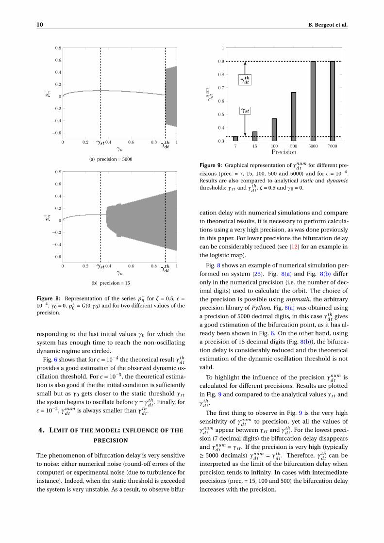
Figure 8: Representation of the series p+n for ζ = 0.5, ε =
10−4, γ0 = 0, p+0 =G(0,γ0) and for two different values of the
precision.
responding to the last initial values γ0 for which the
system has enough time to reach the non-oscillating
dynamic regime are circled.
Fig. 6 shows that for ε= 10−4 the theoretical result γthd t
provides a good estimation of the observed dynamic os-
cillation threshold. For ε= 10−3, the theoretical estima-
tion is also good if the the initial condition is sufficiently
small but as γ0 gets closer to the static threshold γst
the system begins to oscillate before γ= γthd t . Finally, for
ε= 10−2, γnumd t is always smaller than γth
d t .
4. LIMIT OF THE MODEL: INFLUENCE OF THE
PRECISION
The phenomenon of bifurcation delay is very sensitive
to noise: either numerical noise (round-off errors of the
computer) or experimental noise (due to turbulence for
instance). Indeed, when the static threshold is exceeded
the system is very unstable. As a result, to observe bifur-
7 15 100 500 5000 70000.3
0.4
0.5
0.6
0.7
0.8
0.9
1
γthdt
γst
Precision
γnum
dt
Figure 9: Graphical representation of γnumd t for different pre-
cisions (prec. = 7, 15, 100, 500 and 5000) and for ε = 10−4.Results are also compared to analytical static and dynamicthresholds: γst and γth
d t . ζ= 0.5 and γ0 = 0.
cation delay with numerical simulations and compare
to theoretical results, it is necessary to perform calcula-
tions using a very high precision, as was done previously
in this paper. For lower precisions the bifurcation delay
can be considerably reduced (see [12] for an example in
the logistic map).
Fig. 8 shows an example of numerical simulation per-
formed on system (23). Fig. 8(a) and Fig. 8(b) differ
only in the numerical precision (i.e. the number of dec-
imal digits) used to calculate the orbit. The choice of
the precision is possible using mpmath, the arbitrary
precision library of Python. Fig. 8(a) was obtained using
a precision of 5000 decimal digits, in this case γthd t gives
a good estimation of the bifurcation point, as it has al-
ready been shown in Fig. 6. On the other hand, using
a precision of 15 decimal digits (Fig. 8(b)), the bifurca-
tion delay is considerably reduced and the theoretical
estimation of the dynamic oscillation threshold is not
valid.
To highlight the influence of the precision γnumd t is
calculated for different precisions. Results are plotted
in Fig. 9 and compared to the analytical values γst and
γthd t .
The first thing to observe in Fig. 9 is the very high
sensitivity of γnumd t to precision, yet all the values of
γnumd t appear between γst and γth
d t . For the lowest preci-
sion (7 decimal digits) the bifurcation delay disappears
and γnumd t = γst . If the precision is very high (typically
≥ 5000 decimals) γnumd t = γth
d t . Therefore, γthd t can be
interpreted as the limit of the bifurcation delay when
precision tends to infinity. In cases with intermediate
precisions (prec. = 15, 100 and 500) the bifurcation delay
increases with the precision.

Prediction of the dynamic oscillation threshold in a clarinet model with a linearly increasing blowing pressure 11
10−4 10−3 10−20.1
0.2
0.3
0.4
0.5
0.6
0.7
0.8
0.9
1
1.1
1.2
prec. = 5000
prec. = 500
prec. = 100
prec. = 15 prec. = 7
γst
γthdt
ε
γnum
dt
Figure 10: Graphical representation of γnumd t as a function of ε for ζ= 0.5, γ0 = 0 and using five different precisions. A logarithmic
scale is used in abscissa.
The sensitivity to the precision depends on the value
of the increase rate ε: Fig. 10 plots γnumd t with respect to
ε for different values of the numerical precision. Results
are also compared with γst and γthd t .
As above, for the lowest precision (7 decimals) the
bifurcation delay disappears when ε is sufficiently small.
Indeed, γnumd t is constant and equal to γst . Then bifur-
cation delay occurs and increases with ε. The case of
the highest precision (5000 decimals) is identical to an
analytical case which would correspond to infinite pre-
cision. When ε is sufficiently small, the curves of γnumd t
and γthd t overlap. In this case when ε is small γnum
d t is al-
most constant suggesting that the bifurcation delay does
not depend on the increase rate, as previously shown in
Fig. 6(d). Then, still in the case of a precision of 5000
decimals, γnumd t decreases for increasing ε, and γth
d t also
decreases but to a lesser extent. For intermediate preci-
sions (15, 100 and 500 decimals) the curve of γnumd t first
increases before stabilizing close to the curve of γthd t .
For a given value of the precision, the larger the ε,
the smaller is the accumulation of round-off errors cre-
ated by the computer to reach a certain value of γ. This
explains why the bifurcation delay first increases if the
precision is not sufficiently high to simulate an analytic
case. Beyond a certain value, all curves coincide with
the one corresponding to the highest precision. That
means that the system has reached the pair of parame-
ters [precison ; ε] needed to simulate an analytic case.
5. CONCLUSION
When considering mathematical models of musical in-
struments, oscillation threshold obtained through a
static bifurcation analysis may be possibly very different
from the threshold detected on a numerical simulation
of this model.
For the first time for musical instruments, the differ-
ences between these two thresholds have been inter-
preted as the appearance of the phenomenon of bifur-
cation delay in connection with the concept of dynamic
bifurcation.
Theoretical estimations of the dynamic bifurcation
provided in this paper have to be compared with care
to numerical simulations since the numerical precision
used in computations plays a key role: for numerical
precisions close to standard machine precision, the bi-
furcation towards the oscillating regime can occur at sig-
nificantly lower mouth pressure values (while different
most of the time from the threshold obtained through
static bifurcation theory). Moreover, in that case, the
threshold at which the oscillations start becomes more
dependent on the increase rate of the mouth pressure.
The dependency on precision can be linked to the
influence of noise generated by turbulence as the musi-
cian blows into the instrument. This would explain why
the delays observed in artificially blown instruments are
shorter than the predicted theoretical ones [5]. This will
be the subject of further work on this subject, as well
as the validity of these results for smoother curves of
variation of the mouth pressure.
Moreover, in the light of results presented here for a
basic model of wind instruments, varying the blowing
pressure (even slowly) does not appear as the best way
to experimentally determine Hopf bifurcations (static).
In a musical context, since the blowing pressure varies
through time, the dynamic threshold is likely to give
more relevant informations than the static threshold,
even if, in a real situation the influence of noise must

12 B. Bergeot et al.
be considered.
As a final remark, the simplistic model used in this
work only describes one point per half-period of the
sound played by the instrument. It is thus not suitable
to describe different regimes (whose frequencies are har-
monics of the fundamental one) that can be obtained
by the instrument. However a simple extension of this
model calculating the orbits of different instants within
the half-period may be able to provide some insight on
this subject.
acknowledgements
We wish to thank Mr. Jean Kergomard for his valuable
comments on the manuscript.
This work was done within the framework of
the project SDNS-AIMV "Systèmes Dynamiques Non-
Stationnaires - Application aux Instruments à Vent" fi-
nanced by Agence Nationale de la Recherche (ANR).
APPENDIX A. TABLE OF NOTATION
Appendix A.1 Physical variables
Symbol Explanation Unit
Zc characteristic impedance Pa·s·m−3
Ks static stiffness of the reed per
unit area
Pa·m−1
PM static closing pressure of the
reed
Pa
H opening height of the reed
channel at rest
m
U flow created by the pressure
imbalance between the mouth
and the mouthpiece
m3·s−1
Ur flow created by the motion of
the reed
m3·s−1
Ui n flow at the entrance of the res-
onator
m3·s−1
UA flow amplitude parameter m3·s−1
Pm musician mouth pressure Pa
P pressure inside the mouthpiece Pa
∆P pressure difference Pm −P Pa
y displacement of the tip of the
reed
m
τ round trip travel time of a wave
along the resonator
s
Appendix A.2 Dimensionless variables
Symbol Associated physical variable
γ musician mouth pressure
ζ flow amplitude parameter
u flow at the entrance of the resonator
p pressure inside the mouthpiece
r reflexion function of the resonator
p+ outgoing wave
p− incoming wave
p+∗ non-oscillating static regime of p+
(fixed points of the function G)
φ invariant curve
w difference between p+ and φ
ε increase rate of the parameter γ
γst static oscillation threshold
γd t dynamic oscillation threshold
γthd t theoretical estimation of the dynamic
oscillation threshold
γnumd t value of γ when the system begins to
oscillate (calculated numerically)
Appendix A.3 Nonlinear characteristic of the em-bouchure
Function Associated repre-sentation
Definition
F {u ; p} u = F (p)
G {p+ ; p−} p+ =G(−p−)
APPENDIX B. INVARIANT CURVE
The invariant curve φ(γ,ε) is invariant under the map-
ping (23), it therefore satisfies the following equation:
φ(γ,ε) =G(φ(γ−ε,ε),γ
). (40)
First of all, the invariant curve is expanded into a
power series of ε and only he first-order is retained:
φ(γ,ε) ≈φ0(γ)+εφ1(γ). (41)
Secondly, the function G is linearized around the
curve p+∗(γ) of the fixed points:
G(x,γ) ≈ G(p+∗(γ),γ
)+[x −p+∗(γ)
]∂xG
(p+∗(γ),γ
)(42)
= p+∗(γ)+ [x −p+∗(γ)
]∂xG
(p+∗(γ),γ
),(43)
where
∂xG(x, y
)= ∂G(x, y)
∂x. (44)
Then, we make a Taylor expansion of φ(γ−ε,ε):

Prediction of the dynamic oscillation threshold in a clarinet model with a linearly increasing blowing pressure 13
φ(γ−ε,ε) ≈ φ(γ,ε)−ε∂φ∂γ
(γ,ε)+O(ε2); (45)
= φ0(γ)+εφ1(γ)−ε∂φ0(γ)
∂γ+O(ε2).(46)
Finally, neglecting the second-order terms in ε, equa-
tion (40) becomes:
φ0(γ)+εφ1(γ) = p+∗(γ)+[φ0(γ)+εφ1(γ)−ε∂φ0(γ)
∂γ−p+∗(γ)
]×
∂xG(p+∗(γ),γ
). (47)
To obtain the approximate analytical expression of
the invariant cure φ, equation (47) is successively solved
for the functions φ0(γ) and φ1(γ).
As expected, to order 0 we find:
φ0(γ) = p+∗(γ). (48)
To order 1, we have to solve:
φ1(γ) =[φ1(γ)− ∂φ0(γ)
∂γ
]∂xG
(p+∗(γ),γ
); (49)
=[φ1(γ)− ∂p+∗(γ)
∂γ
]∂xG
(p+∗(γ),γ
), (50)
and therefore:
φ1(γ) = ∂p+∗(γ)
∂γ
∂xG(p+∗(γ),γ
)∂xG
(p+∗(γ),γ
)−1. (51)
Finally the expression of the invariant curve is:
φ(γ,ε) ≈
p+∗(γ) + ε∂p+∗(γ)
∂γ
∂xG(p+∗(γ),γ
)∂xG
(p+∗(γ),γ
)−1. (52)
REFERENCES
[1] Atig, M., Dalmont, J.P., Gilbert, J.: Saturation mech-
anism in clarinet-like instruments, the effect of the
localised nonlinear losses. Appl. Acoust. 65(12),
1133–1154 (2004)
[2] Baesens, C.: Slow sweep through a period-doubling
cascade: Delayed bifurcations and renormalisation.
Physica D 53, 319–375 (1991)
[3] Baesens, C.: Gevrey series and dynamic bifurca-
tions for analytic slow-fast mappings. Nonlinearity
8, 179–201 (1995)
[4] Bender, C., Orszag, S.: Advanced mathematical
methods for scientists and engineers. McGraw-Hill
Book Company (1987)
[5] Bergeot, B., Vergez, C., Almeida, A., Gazengel, B.:
Measurement of attack transients in a clarinet
driven by a ramp-like varying pressure. In: 11ème
Congrès Français d’Acoustique and 2012 Annual
IOA Meeting (Nantes, France, April 23rd-27th 2012)
[6] Chaigne, A., Kergomard, J.: Instruments à an-
che. In: Acoustique des instruments de musique,
chap. 9, pp. 400–468. Belin (2008)
[7] Dalmont, J., Gilbert, J., Kergomard, J., Ollivier, S.:
An analytical prediction of the oscillation and ex-
tinction thresholds of a clarinet. J. Acoust. Soc. Am.
118(5), 3294–3305 (2005)
[8] Feigenbaum, M.J.: The universal metric properties
of nonlinear transformations. J. Stat. Phy. 21(6),
669–706 (1979)
[9] Ferrand, D., Vergez, C., Silva, F.: Seuils d’oscillation
de la clarinette : validité de la représentation
excitateur-résonateur. In: 10ème Congrès Français
d’Acoustique (Lyon, France, April 12nd-16th 2010)
[10] Fruchard, A.: Canards et râteaux. Ann. Inst. Fourier
42(4), 825–855 (1992)
[11] Fruchard, A.: Sur l’équation aux différences affine
du premier ordre unidimensionnelle. Ann. Inst.
Fourier 46(1), 139–181 (1996)
[12] Fruchard, A., Schäfke, R.: Bifurcation delay and
difference equations. Nonlinearity 16, 2199–2220
(2003)
[13] Fruchard, A., Schäfke, R.: Sur le retard à
la bifurcation. In: International confer-
ence in honor of claude Lobry (2007). URL
http://intranet.inria.fr/international/arima/009/pdf/arima00925.pdf
[14] Hirschberg, A.: Aero-acoustics of wind instru-
ments. In: Mechanics of musical instruments by A.
Hirschberg/ J. Kergomard/ G. Weinreich, vol. 335
of CISM Courses and lectures, chap. 7, pp. 291–361.
Springer-Verlag (1995)
[15] Hirschberg, A., de Laar, R.W.A.V., Maurires, J.P., Wij-
nands, A.P.J., Dane, H.J., Kruijswijk, S.G., Houtsma,

14 B. Bergeot et al.
A.J.M.: A quasi-stationary model of air flow in the
reed channel of single-reed woodwind instruments.
Acustica 70, 146–154 (1990)
[16] Kapral, R., Mandel, P.: Bifurcation structure of the
nonautonomous quadratic map. Phys. Rev. A 32(2),
1076–1081 (1985)
[17] Kergomard, J.: Elementary considerations on reed-
instrument oscillations. In: Mechanics of musi-
cal instruments by A. Hirschberg/ J. Kergomard/ G.
Weinreich, vol. 335 of CISM Courses and lectures,
chap. 6, pp. 229–290. Springer-Verlag (1995)
[18] Kergomard, J., Dalmont, J.P., Gilbert, J., Guillemain,
P.: Period doubling on cylindrical reed instruments.
In: Proceeding of the Joint congress CFA/DAGA
04, pp. 113–114. Société Française d’Acoustique
- Deutsche Gesellschaft für Akustik (2004, Stras-
bourg, France)
[19] Kuznetsov, Y.A.: Elements of Applied Bifurcation
Theory, vol. 112, 3rd edn. chap. 4, p. 136, Springer
(2004)
[20] Maganza, C., Caussé, R., Laloë, F.: Bifurcations, pe-
riod doublings and chaos in clarinet-like systems.
EPL (Europhysics Letters) 1(6), 295 (1986)
[21] Mcintyre, M.E., Schumacher, R.T., Woodhouse, J.:
On the oscillations of musical instruments. J.
Acoust. Soc. Am. 74(5), 1325–1345 (1983)
[22] Ollivier, S., Dalmont, J.P., Kergomard, J.: Idealized
models of reed woodwinds. part 2 : On the stability
of two-step oscillations. Acta. Acust. united Ac. 91,
166–179 (2005)
[23] Taillard, P., Kergomard, J., Laloë, F.: Iterated maps
for clarinet-like systems. Nonlinear Dyn. 62, 253–
271 (2010)
[24] Tredicce, J.R., Lippi, G., Mandel, P., Charasse, B.,
Chevalier, A., Picqué, B.: Critical slowing down at a
bifurcation. Am. J. Phys. 72(6), 799–809 (2004)
[25] Wilson, T., Beavers, G.: Operating modes of the
clarinet. J. Acoust. Soc. Am. 56(2), 653–658 (1974)