Embed Size (px)
Citation preview
Clark
Opening Thoughts
Outside of a few technical sections, this is a very process-oriented paper. Practice problems are
key!
Outline
I. Introduction
� Objectives in creating a formal model of loss reserving:
• Describe loss emergence in simple mathematical terms as a guide to selecting amounts
for carried reserves
• Provide a means of estimating the range of possible outcomes around the “expected”
reserve
� A statistical loss reserving model has two key elements:
• The expected amount of loss to emerge in some time period
• The distribution of actual emergence around the expected value
II. Expected Loss Emergence
� Model will estimate the expected amount of loss to emerge based on:
• An estimate of the ultimate loss by year
• An estimate of the pattern of loss emergence
� Let G(x) = 1/LDFx be the cumulative % of loss reported (or paid) as of time x, where x
represents the time (in months) from the “average” accident date to the evaluation date
� Assume that the loss emergence pattern is described by one of the following curves with
scale θ and shape ω
• Loglogistic
G(x|ω, θ) =xω
xω + θω
LDFx = 1 + θω · x−ω
c©2014 A Casual Fellow’s Exam Seminars 201 2015 CAS Exam 7
Clark
• Weibull
G(x|ω, θ) = 1− exp(−(x/θ)ω)
� With these curves, we assume a strictly increasing pattern. If there is real expected negative
development (salvage recoveries), different models should be used
� Advantages to using parameterized curves to describe the emergence pattern:
• Estimation is simple since we only have to estimate two parameters
• We can use data that is not from a triangle with evenly spaced evaluation data – such
as the case in which the latest diagonal is only nine months from the second latest
diagonal
• The final pattern is smooth and does not follow random movements in the historical
age-to-age factors
� In order to estimate the loss emergence amount, we require an estimate of the ultimate loss
by AY. There are two methods described in the paper:
• LDF method – assumes the loss amount in each AY is independent from all other years
(this is the standard chain-ladder method)
• Cape Cod method – assumes that there is a known relationship between expected
ultimate losses across accident years, where the relationship is identified by an exposure
base (on-level premium, sales, payroll, etc.)
� Let µAY ;x,y = expected incremental loss dollars in accident year AY between ages x and y
� Combining the loss emergence pattern with the estimate of the ultimate loss by year, we
obtain the following for each method:
• LDF method
µAY ;x,y = ULTAY · [G(y|ω, θ)−G(x|ω, θ)]
• Cape Cod method
µAY ;x,y = PremiumAY · ELR · [G(y|ω, θ)−G(x|ω, θ)]
� In general, the Cape Cod method is preferred since data is summarized into a loss triangle
with relatively few data points. Since the LDF method requires an estimation of a number
of parameters (one for each AY ultimate loss, as well as θ and ω), it tends to be over-
parameterized when few data points exist
� Due to the additional information given by the exposure base (as well as fewer parameters),
the Cape Cod method has a smaller parameter variance. The process variance can be higher
2015 CAS Exam 7 202 c©2014 A Casual Fellow’s Exam Seminars

Clark
or lower than the LDF method. In general, the Cape Cod method produces a lower total
variance than the LDF method
III. The Distribution of Actual Loss Emergence and Maximum Likelihood
� The variance of the actual loss emergence can be estimated in two pieces: process variance
(the “random” amount) and parameter variance (the uncertainty in the estimator, also
known as the estimation error)
� Process variance
• Assume that the loss in any period has a constant ratio of variance/mean:
Variance
Mean= σ2 ≈ 1
n− p
n∑AY,t
(cAY,t − µAY,t)2
µAY,t
where n = # of data points, p = # of parameters, cAY,t = actual incremental loss
emergence and µAY,t = expected incremental loss emergence
• For estimating the parameters of our model, let’s assume that the actual loss emergence
“c” follows an over-dispersed Poisson distribution with scaling factor σ2
• Assuming λ represents the mean of a standard Poisson random variable, the mean and
variance of an over-dispersed Poisson are as follows:
� E[c] = λσ2 = µ
� V ar(c) = λσ4 = µσ2
• Key advantages of using the over-dispersed Poisson distribution:
� Inclusion of scaling factors allows us to match the first and second moments of
any distribution, allowing high flexibility
� Maximum likelihood estimation produces the LDF and Cape Cod estimates of
ultimate losses, so the results can be presented in a familiar format
� The likelihood function
• For an over-dispersed Poisson distribution, the Pr(c) = λc/σ2e−λ
(c/σ2)!
• Likelihood =∏i
Pr(ci) =∏i
λci/σ
2
i e−λi
(ci/σ2)!=∏i
(µi/σ2)ci/σ
2e−(µi/σ
2)
(ci/σ2)!
• After taking the log of the likelihood function above, we obtain the loglikelihood, l,
which we need to maximize:
l =∑i
ci · ln(µi)− µi
c©2014 A Casual Fellow’s Exam Seminars 203 2015 CAS Exam 7
Clark
• Before applying this loglikelihood formula to our two methods, let’s define a few things:
� ci,t = actual loss in AY i, development period t
� Pi = premium for AY i
� xt−1 = beginning age for development period t
� xt = ending age for development period t
• LDF method
� Taking the derivative of l and setting it equal to zero yields the following MLE
estimate for ULTi:
ULTi =
∑tci,t∑
t[G(xt)−G(xt−1)]
� The MLE estimate for each ULTi is equivalent to the “LDF Ultimate”
• Cape Cod method
� Taking the derivative of l and setting it equal to zero yields the following MLE
estimate for the ELR:
ELR =
∑i,tci,t∑
i,tPi · [G(xt)−G(xt−1)]
� The MLE estimate for the ELR is equivalent to the “Cape Cod” Ultimate
• An advantage of the maximum loglikelihood function is that it works in the presence
of negative or zero incremental losses (since we never actually take the log of ci,t)
� Parameter variance
• We need the covariance matrix (inverse of the information matrix) to calculate the
parameter variance
• Due to the complexity involved (it would be downright impossible for the LDF method),
I don’t expect you will need to calculate the parameter variance on the exam
� Variance of the reserves
• As usual, in order to calculate the variance of an estimate of loss reserves R, we need
the process variance and parameter variance:
� Process Variance of R = σ2 ·∑µAY ;x,y
� Parameter Variance of R = too complicated for the exam
2015 CAS Exam 7 204 c©2014 A Casual Fellow’s Exam Seminars
Clark
IV. Key Assumptions of this Model
� Assumption 1: Incremental losses are independent and identically distributed (iid)
• “Independence” means that one period does not affect the surrounding periods
� Can be tested using residual analysis
� Positive correlation could exist if all periods are equally impacted by a change
in loss inflation
� Negative correlation could exist if a large settlement in one period replaces a
stream of payments in later periods
• “Identically distributed” assumes that the emergence pattern is the same for all acci-
dent years, which is clearly over-simplified
� Different risks and a different mix of business would have been written in each
historical period, each subject to different claims handling and settlement prac-
tices
� Assumption 2: The variance/mean scale parameter σ2 is fixed and known
• Technically, σ2 should be estimated simultaneously with the other model parameters,
with the variance around its estimate included in the covariance matrix
• However, doing so results in messy mathematics. For convenience and simplicity, we
assume that σ2 is fixed and known
� Assumption 3: Variance estimates are based on an approximation to the Rao-Cramer lower
bound
• The estimate of variance based on the information matrix is only exact when we are
using linear functions
• Since our model is non-linear, the variance estimate is a Rao-Cramer lower bound (i.e.
the variance estimate is as low as it possibly can be)
V. A Practical Example
� In the paper, Clark applies his methodology to 10 x 10 triangle. To simplify things, we will be
studying a 5 x 5 triangle. In general, this example will focus on estimating the reserves using
the LDF and Cape Cod methods. For the more detailed calculations (such as determining
model parameters or calculating residuals), see the Clark Example excel spreadsheet on the
website. The Clark Example spreadsheet includes the giant example found in the text as
well
c©2014 A Casual Fellow’s Exam Seminars 205 2015 CAS Exam 7
Clark
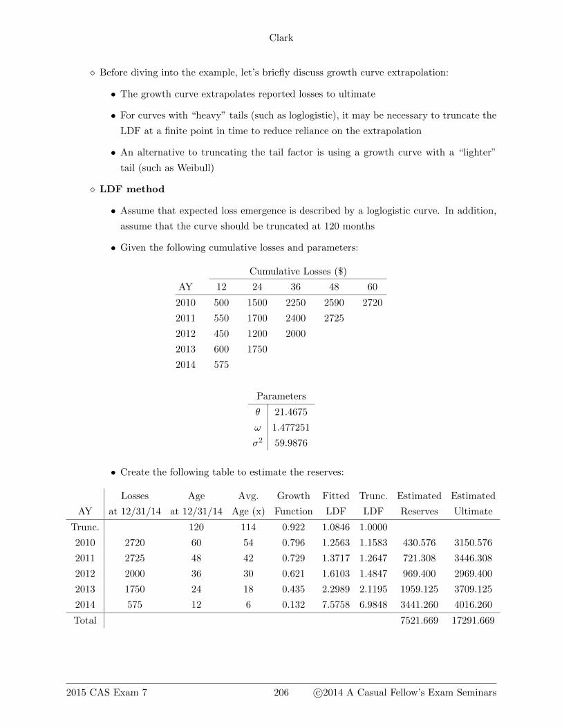
� Before diving into the example, let’s briefly discuss growth curve extrapolation:
• The growth curve extrapolates reported losses to ultimate
• For curves with “heavy” tails (such as loglogistic), it may be necessary to truncate the
LDF at a finite point in time to reduce reliance on the extrapolation
• An alternative to truncating the tail factor is using a growth curve with a “lighter”
tail (such as Weibull)
� LDF method
• Assume that expected loss emergence is described by a loglogistic curve. In addition,
assume that the curve should be truncated at 120 months
• Given the following cumulative losses and parameters:
Cumulative Losses ($)
AY 12 24 36 48 60
2010 500 1500 2250 2590 2720
2011 550 1700 2400 2725
2012 450 1200 2000
2013 600 1750
2014 575
Parameters
θ 21.4675
ω 1.477251
σ2 59.9876
• Create the following table to estimate the reserves:
Losses Age Avg. Growth Fitted Trunc. Estimated Estimated
AY at 12/31/14 at 12/31/14 Age (x) Function LDF LDF Reserves Ultimate
Trunc. 120 114 0.922 1.0846 1.0000
2010 2720 60 54 0.796 1.2563 1.1583 430.576 3150.576
2011 2725 48 42 0.729 1.3717 1.2647 721.308 3446.308
2012 2000 36 30 0.621 1.6103 1.4847 969.400 2969.400
2013 1750 24 18 0.435 2.2989 2.1195 1959.125 3709.125
2014 575 12 6 0.132 7.5758 6.9848 3441.260 4016.260
Total 7521.669 17291.669
2015 CAS Exam 7 206 c©2014 A Casual Fellow’s Exam Seminars
Clark
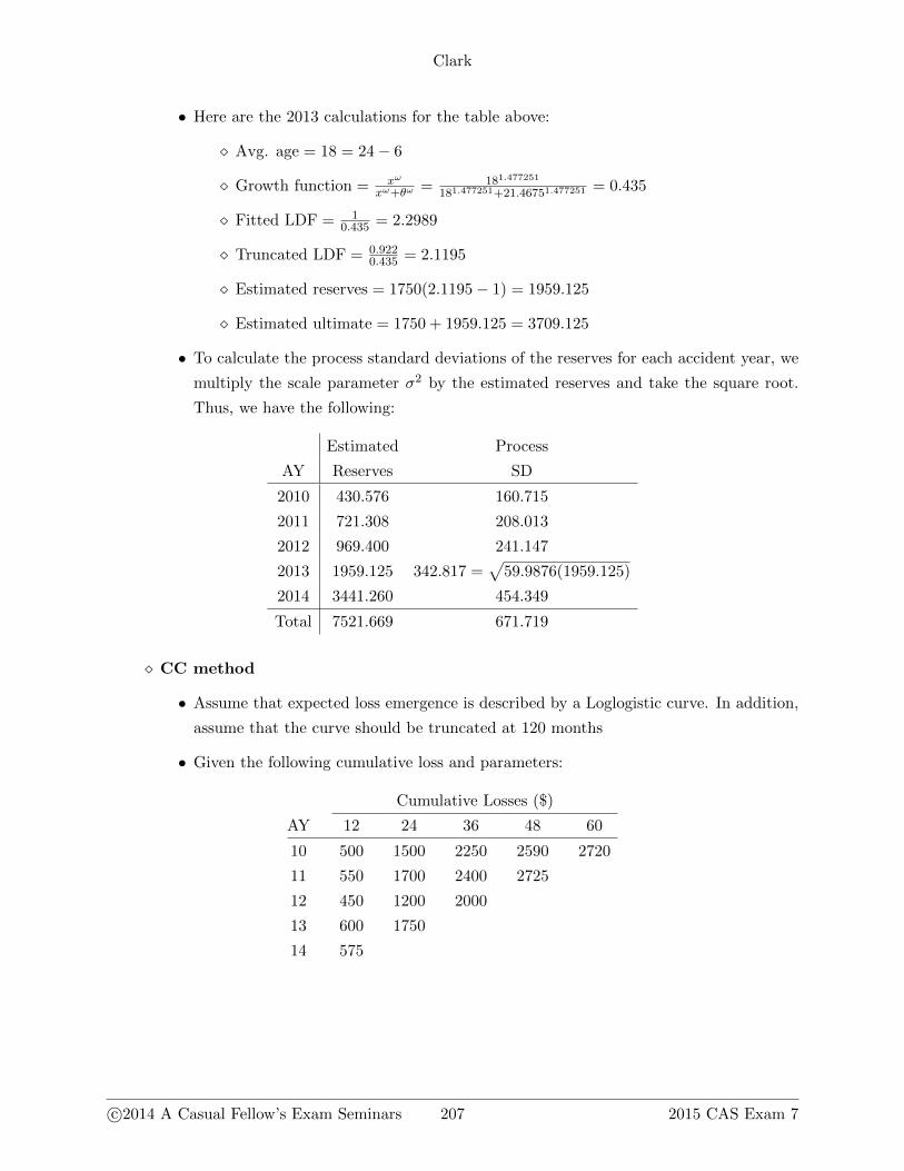
• Here are the 2013 calculations for the table above:
� Avg. age = 18 = 24− 6
� Growth function = xω
xω+θω = 181.477251
181.477251+21.46751.477251= 0.435
� Fitted LDF = 10.435 = 2.2989
� Truncated LDF = 0.9220.435 = 2.1195
� Estimated reserves = 1750(2.1195− 1) = 1959.125
� Estimated ultimate = 1750 + 1959.125 = 3709.125
• To calculate the process standard deviations of the reserves for each accident year, we
multiply the scale parameter σ2 by the estimated reserves and take the square root.
Thus, we have the following:
Estimated Process
AY Reserves SD
2010 430.576 160.715
2011 721.308 208.013
2012 969.400 241.147
2013 1959.125 342.817 =√
59.9876(1959.125)
2014 3441.260 454.349
Total 7521.669 671.719
� CC method
• Assume that expected loss emergence is described by a Loglogistic curve. In addition,
assume that the curve should be truncated at 120 months
• Given the following cumulative loss and parameters:
Cumulative Losses ($)
AY 12 24 36 48 60
10 500 1500 2250 2590 2720
11 550 1700 2400 2725
12 450 1200 2000
13 600 1750
14 575
c©2014 A Casual Fellow’s Exam Seminars 207 2015 CAS Exam 7
Clark
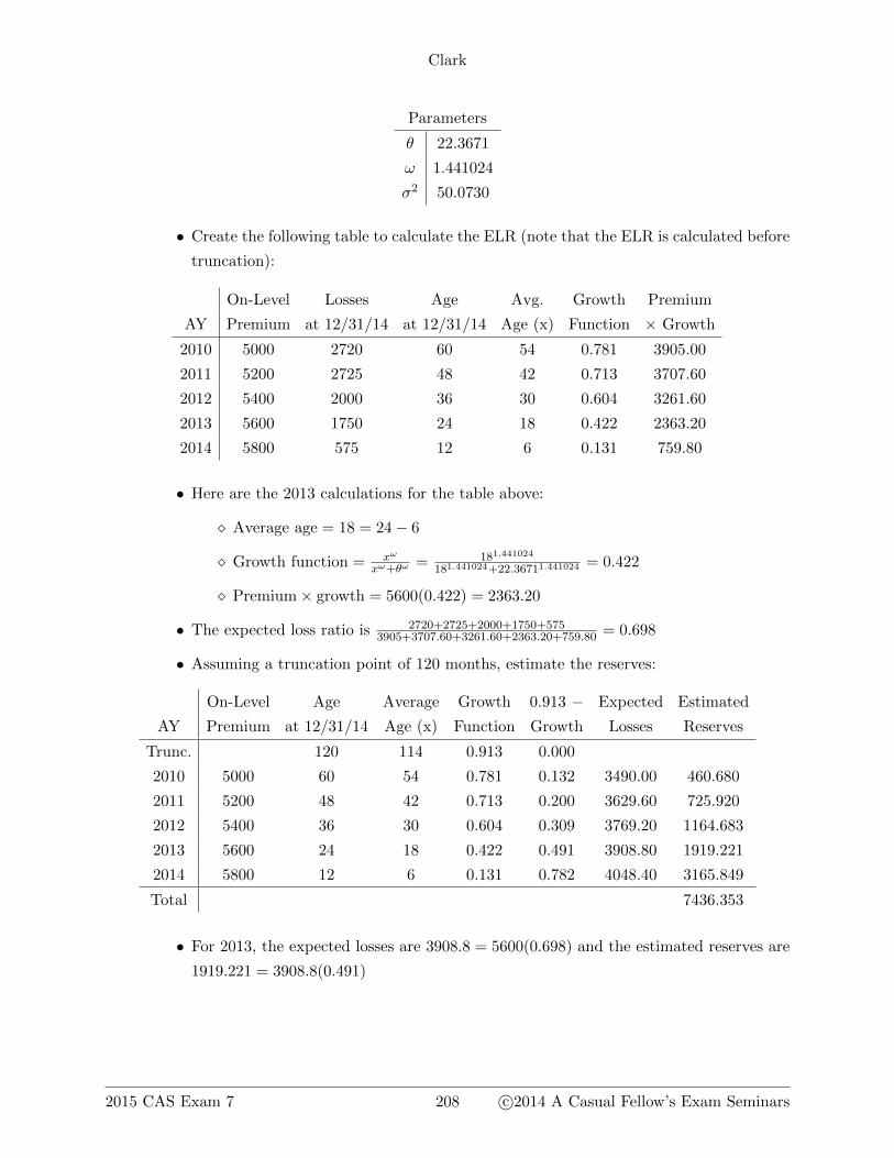
Parameters
θ 22.3671
ω 1.441024
σ2 50.0730
• Create the following table to calculate the ELR (note that the ELR is calculated before
truncation):
On-Level Losses Age Avg. Growth Premium
AY Premium at 12/31/14 at 12/31/14 Age (x) Function × Growth
2010 5000 2720 60 54 0.781 3905.00
2011 5200 2725 48 42 0.713 3707.60
2012 5400 2000 36 30 0.604 3261.60
2013 5600 1750 24 18 0.422 2363.20
2014 5800 575 12 6 0.131 759.80
• Here are the 2013 calculations for the table above:
� Average age = 18 = 24− 6
� Growth function = xω
xω+θω = 181.441024
181.441024+22.36711.441024= 0.422
� Premium× growth = 5600(0.422) = 2363.20
• The expected loss ratio is 2720+2725+2000+1750+5753905+3707.60+3261.60+2363.20+759.80 = 0.698
• Assuming a truncation point of 120 months, estimate the reserves:
On-Level Age Average Growth 0.913 − Expected Estimated
AY Premium at 12/31/14 Age (x) Function Growth Losses Reserves
Trunc. 120 114 0.913 0.000
2010 5000 60 54 0.781 0.132 3490.00 460.680
2011 5200 48 42 0.713 0.200 3629.60 725.920
2012 5400 36 30 0.604 0.309 3769.20 1164.683
2013 5600 24 18 0.422 0.491 3908.80 1919.221
2014 5800 12 6 0.131 0.782 4048.40 3165.849
Total 7436.353
• For 2013, the expected losses are 3908.8 = 5600(0.698) and the estimated reserves are
1919.221 = 3908.8(0.491)
2015 CAS Exam 7 208 c©2014 A Casual Fellow’s Exam Seminars
Clark
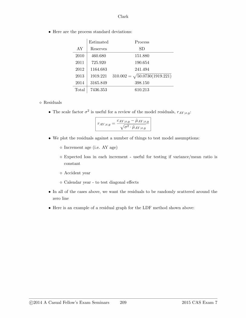
• Here are the process standard deviations:
Estimated Process
AY Reserves SD
2010 460.680 151.880
2011 725.920 190.654
2012 1164.683 241.494
2013 1919.221 310.002 =√
50.0730(1919.221)
2014 3165.849 398.150
Total 7436.353 610.213
� Residuals
• The scale factor σ2 is useful for a review of the model residuals, rAY ;x,y:
rAY ;x,y =cAY ;x,y − µ̂AY ;x,y√
σ2 · µ̂AY ;x,y
• We plot the residuals against a number of things to test model assumptions:
� Increment age (i.e. AY age)
� Expected loss in each increment - useful for testing if variance/mean ratio is
constant
� Accident year
� Calendar year - to test diagonal effects
• In all of the cases above, we want the residuals to be randomly scattered around the
zero line
• Here is an example of a residual graph for the LDF method shown above:
c©2014 A Casual Fellow’s Exam Seminars 209 2015 CAS Exam 7
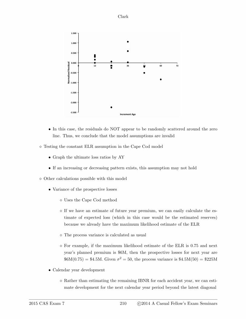
Clark
!"#$%%&
!"#%%%&
!'#$%%&
!'#%%%&
!%#$%%&
%#%%%&
%#$%%&
'#%%%&
'#$%%&
%& '"& "(& )*& (+& *%& ,"&
-./0
123456&75836912&
:;</505;=&>?5&
• In this case, the residuals do NOT appear to be randomly scattered around the zero
line. Thus, we conclude that the model assumptions are invalid
� Testing the constant ELR assumption in the Cape Cod model
• Graph the ultimate loss ratios by AY
• If an increasing or decreasing pattern exists, this assumption may not hold
� Other calculations possible with this model
• Variance of the prospective losses
� Uses the Cape Cod method
� If we have an estimate of future year premium, we can easily calculate the es-
timate of expected loss (which in this case would be the estimated reserves)
because we already have the maximum likelihood estimate of the ELR
� The process variance is calculated as usual
� For example, if the maximum likelihood estimate of the ELR is 0.75 and next
year’s planned premium is $6M, then the prospective losses for next year are
$6M(0.75) = $4.5M. Given σ2 = 50, the process variance is $4.5M(50) = $225M
• Calendar year development
� Rather than estimating the remaining IBNR for each accident year, we can esti-
mate development for the next calendar year period beyond the latest diagonal
2015 CAS Exam 7 210 c©2014 A Casual Fellow’s Exam Seminars
Clark
� To estimate development for the next 12-month calendar period, we take the
difference in growth functions at the two evaluation ages and multiply it by the
estimated ultimate losses
� The process variance and parameter variance are calculated as usual
� A major reason for calculating the 12-month development is that the estimate
is testable within a short timeframe. One year later, we can compare it to the
actual development and see if it was within the forecast range
• Variability in discounted reserves
� Use the same payout pattern and model parameters that were used with undis-
counted reserves
� The CV for discounted reserves is lower since the tail of the payout curve has
the greatest parameter variance and also receives the deepest discount
� See Appendix C section below for the calculation of discounted reserves, as well
as an example
VI. Comments and Conclusion
� Abandon your triangles
• The MLE model works best when using a tabular format of data (see exhibits in paper
for an example) rather than a triangular format
• All we need is a consistent aggregation of losses evaluated at more than one date
� The CV goes with the mean
• If we selected a carried reserve other than the maximum likelihood estimate, can we
still use the CV from the model?
� Technically, the answer is “no”. The estimate of the standard deviation in the
MLE model is directly tied to the maximum likelihood estimate
� However, for practical purposes, the answer is “yes”. Since the final carried
reserve is a selection based on a number of factors (some of which are not captured
in the model), it stands to reason that the standard deviation should also be a
selection. The output from the MLE model is a reasonable basis for that selection
� Other curve forms
• This paper focused on the loglogistic and weibull growth curves for a few reasons:
� Smoothly move from 0% to 100%
c©2014 A Casual Fellow’s Exam Seminars 211 2015 CAS Exam 7
Clark
� Closely match the empirical data
� First and second derivatives are calculable
• The method is not limited to these forms; other curves could be used
� The main conclusion of the paper is that parameter variance is generally larger
than the process variance, implying that our need for more complete data (such as the
exposure information in the Cape Cod method) outweighs the need for more sophisticated
models
VII. Appendix B: Adjustments for Different Exposure Periods
� Before showing the final formula, let’s walk through a quick example:
• Assume we are 9 months into an accident year
• Then G∗(4.5|ω, θ) represents the cumulative percent of ultimate of the 9-month period
only (not the entire AY since a full AY exposure period is 12 months)
• In order to estimate the cumulative percent of ultimate for the full accident year, we
must multiply by a scaling factor that represents the portion of the AY that has been
earned
• Thus, the AY cumulative percent of ultimate as of 9 months is GAY (9|ω, θ) =
( 912) ·G∗(4.5|ω, θ)
� Generalizing this process, there are two steps:
• Step 1: Calculate the percent of the period that is exposed:
For accident years (AY):
Expos(t) =
t/12, t ≤ 12
1, t > 12
• Step 2: Calculate the average accident date of the period that is earned:
For accident years (AY):
AvgAge(t) =
t/2, t ≤ 12
t− 6, t > 12
� The final cumulative percent of ultimate curve, including annualization, is given by:
GAY (t|ω, θ) = Expos(t) ·G∗(AvgAge(t)|ω, θ)
2015 CAS Exam 7 212 c©2014 A Casual Fellow’s Exam Seminars
Clark
� Note: Since the PY versions of the formulas above are unlikely to be tested, I have not
included them
VIII. Appendix C: Variance in Discounted Reserves
� Calculation of the discounted reserve, Rd:
Rd =∑AY
y−x∑k=1
ULTAY · vk−12 · (G(x+ k)−G(x+ k − 1))
where v = 11+i and i is the constant discount rate
� Process variance of Rd:
V ar(Rd) = σ2 ·∑AY
y−x∑k=1
ULTAY · v2k−1 · (G(x+ k)−G(x+ k − 1))
� LDF method
• For consistency, we will use the same LDF example shown earlier in the outline. Assume
that expected loss emergence is described by a loglogistic curve. In addition, assume
that the curve should be truncated at 120 months
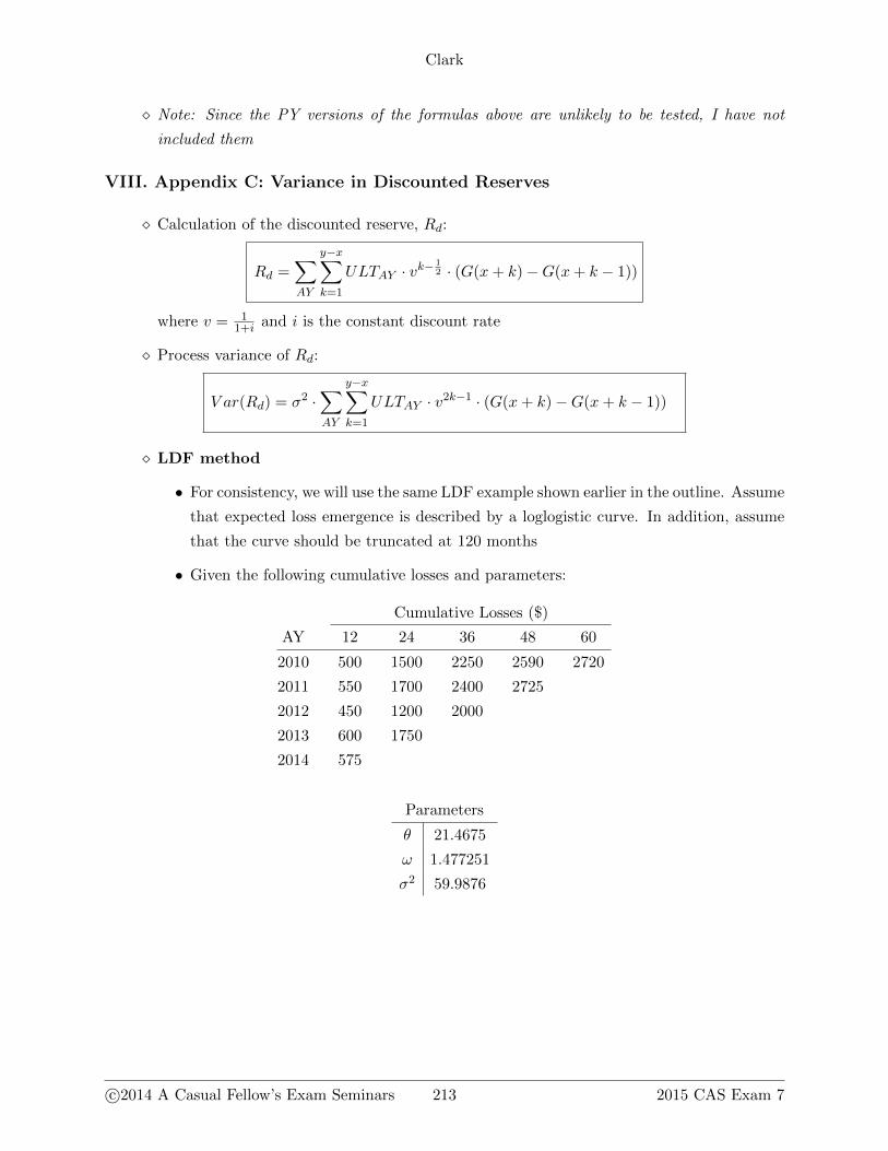
• Given the following cumulative losses and parameters:
Cumulative Losses ($)
AY 12 24 36 48 60
2010 500 1500 2250 2590 2720
2011 550 1700 2400 2725
2012 450 1200 2000
2013 600 1750
2014 575
Parameters
θ 21.4675
ω 1.477251
σ2 59.9876
c©2014 A Casual Fellow’s Exam Seminars 213 2015 CAS Exam 7
Clark
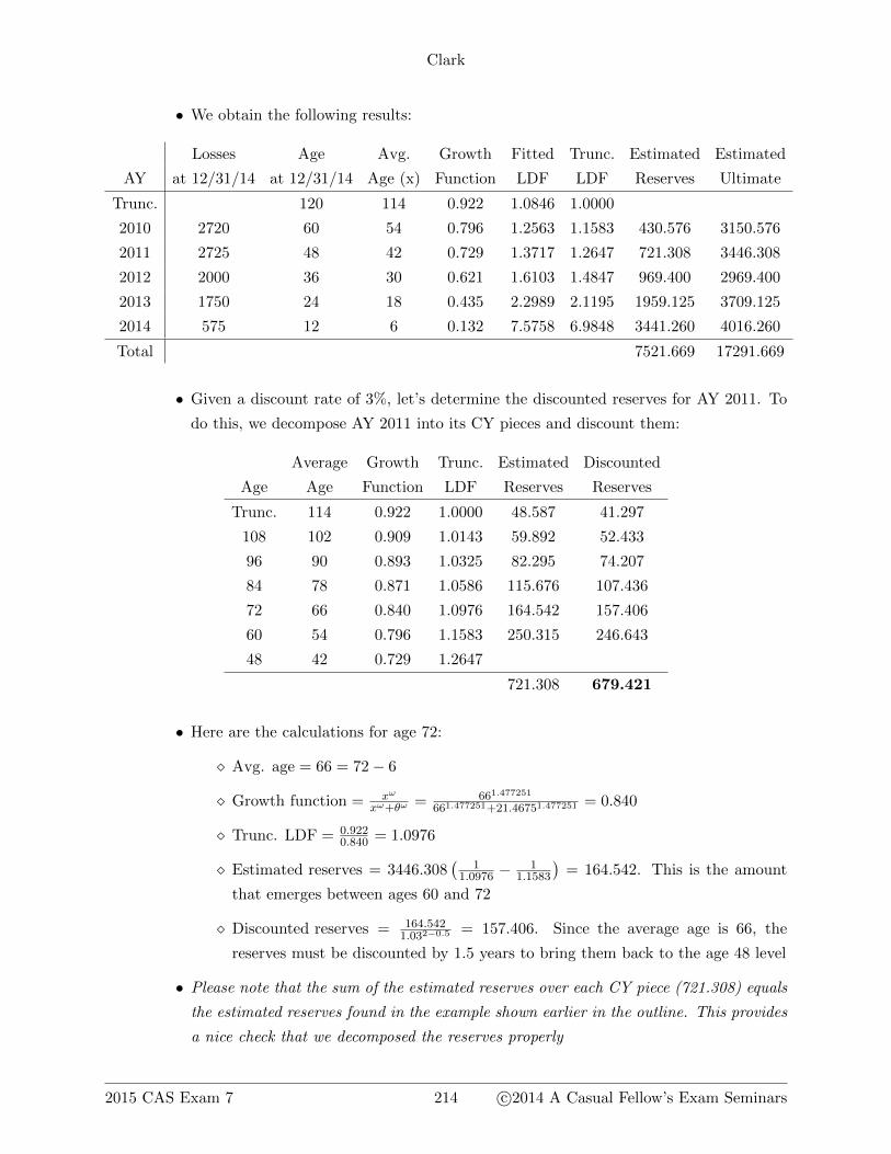
• We obtain the following results:
Losses Age Avg. Growth Fitted Trunc. Estimated Estimated
AY at 12/31/14 at 12/31/14 Age (x) Function LDF LDF Reserves Ultimate
Trunc. 120 114 0.922 1.0846 1.0000
2010 2720 60 54 0.796 1.2563 1.1583 430.576 3150.576
2011 2725 48 42 0.729 1.3717 1.2647 721.308 3446.308
2012 2000 36 30 0.621 1.6103 1.4847 969.400 2969.400
2013 1750 24 18 0.435 2.2989 2.1195 1959.125 3709.125
2014 575 12 6 0.132 7.5758 6.9848 3441.260 4016.260
Total 7521.669 17291.669
• Given a discount rate of 3%, let’s determine the discounted reserves for AY 2011. To
do this, we decompose AY 2011 into its CY pieces and discount them:
Average Growth Trunc. Estimated Discounted
Age Age Function LDF Reserves Reserves
Trunc. 114 0.922 1.0000 48.587 41.297
108 102 0.909 1.0143 59.892 52.433
96 90 0.893 1.0325 82.295 74.207
84 78 0.871 1.0586 115.676 107.436
72 66 0.840 1.0976 164.542 157.406
60 54 0.796 1.1583 250.315 246.643
48 42 0.729 1.2647
721.308 679.421
• Here are the calculations for age 72:
� Avg. age = 66 = 72− 6
� Growth function = xω
xω+θω = 661.477251
661.477251+21.46751.477251= 0.840
� Trunc. LDF = 0.9220.840 = 1.0976
� Estimated reserves = 3446.308(
11.0976 −
11.1583
)= 164.542. This is the amount
that emerges between ages 60 and 72
� Discounted reserves = 164.5421.032−0.5 = 157.406. Since the average age is 66, the
reserves must be discounted by 1.5 years to bring them back to the age 48 level
• Please note that the sum of the estimated reserves over each CY piece (721.308) equals
the estimated reserves found in the example shown earlier in the outline. This provides
a nice check that we decomposed the reserves properly
2015 CAS Exam 7 214 c©2014 A Casual Fellow’s Exam Seminars

Clark
� CC method
• Given the following parameters for the CC method:
Parameters
θ 22.3671
ω 1.441024
σ2 50.0730
• As shown earlier in the outline, we obtain the following results:
On-Level Age Average Growth 0.913 − Expected Estimated
AY Premium at 12/31/14 Age (x) Function Growth Losses Reserves
Trunc. 120 114 0.913 0.000
2010 5000 60 54 0.781 0.132 3490.00 460.680
2011 5200 48 42 0.713 0.200 3629.60 725.920
2012 5400 36 30 0.604 0.309 3769.20 1164.683
2013 5600 24 18 0.422 0.491 3908.80 1919.221
2014 5800 12 6 0.131 0.782 4048.40 3165.849
Total 7436.353
• Given a discount rate of 3%, let’s determine the discounted reserves for AY 2011. To
do this, we decompose AY 2011 into its CY pieces and discount them:
Average Growth 0.913 − Trunc. Estimated Discounted
Age Age Function Growth Growth Reserves Reserves
Trunc. 114 0.913 0.000 1.000 50.814 43.190
108 102 0.899 0.014 0.986 65.333 57.196
96 90 0.881 0.032 0.968 83.481 75.276
84 78 0.858 0.055 0.945 116.147 107.874
72 66 0.826 0.087 0.913 163.332 156.248
60 54 0.781 0.132 0.868 246.813 243.192
48 42 0.713 0.200 0.800
725.920 682.976
• Here are the calculations for age 72:
� Avg. age = 66 = 72− 6
� Growth function = xω
xω+θω = 661.441024
661.441024+22.36711.441024= 0826
� 0.913− Growth = 0.913 - 0.826 = 0.087
c©2014 A Casual Fellow’s Exam Seminars 215 2015 CAS Exam 7
Clark
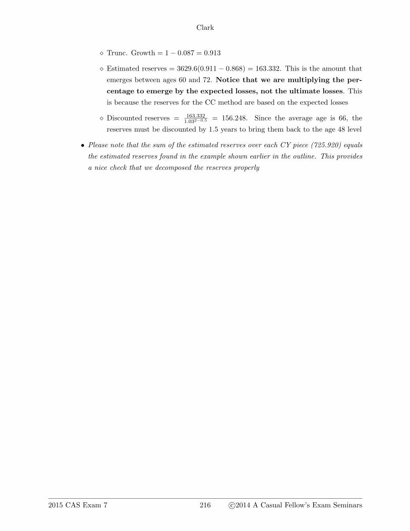
� Trunc. Growth = 1− 0.087 = 0.913
� Estimated reserves = 3629.6(0.911− 0.868) = 163.332. This is the amount that
emerges between ages 60 and 72. Notice that we are multiplying the per-
centage to emerge by the expected losses, not the ultimate losses. This
is because the reserves for the CC method are based on the expected losses
� Discounted reserves = 163.3321.032−0.5 = 156.248. Since the average age is 66, the
reserves must be discounted by 1.5 years to bring them back to the age 48 level
• Please note that the sum of the estimated reserves over each CY piece (725.920) equals
the estimated reserves found in the example shown earlier in the outline. This provides
a nice check that we decomposed the reserves properly
2015 CAS Exam 7 216 c©2014 A Casual Fellow’s Exam Seminars
Clark
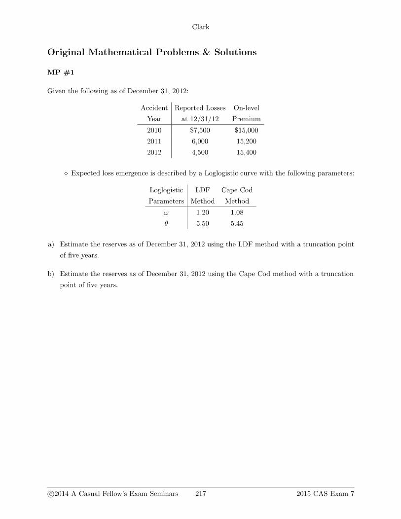
Original Mathematical Problems & Solutions
MP #1
Given the following as of December 31, 2012:
Accident Reported Losses On-level
Year at 12/31/12 Premium
2010 $7,500 $15,000
2011 6,000 15,200
2012 4,500 15,400
� Expected loss emergence is described by a Loglogistic curve with the following parameters:
Loglogistic LDF Cape Cod
Parameters Method Method
ω 1.20 1.08
θ 5.50 5.45
a) Estimate the reserves as of December 31, 2012 using the LDF method with a truncation point
of five years.
b) Estimate the reserves as of December 31, 2012 using the Cape Cod method with a truncation
point of five years.
c©2014 A Casual Fellow’s Exam Seminars 217 2015 CAS Exam 7
Clark
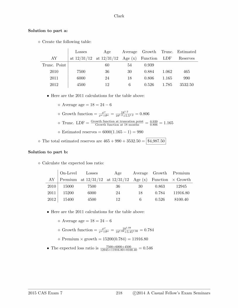
Solution to part a:
� Create the following table:
Losses Age Average Growth Trunc. Estimated
AY at 12/31/12 at 12/31/12 Age (x) Function LDF Reserves
Trunc. Point 60 54 0.939
2010 7500 36 30 0.884 1.062 465
2011 6000 24 18 0.806 1.165 990
2012 4500 12 6 0.526 1.785 3532.50
• Here are the 2011 calculations for the table above:
� Average age = 18 = 24− 6
� Growth function = xω
xω+θω = 181.2
181.2+5.51.2= 0.806
� Trunc. LDF = Growth function at truncation pointGrowth function at 18 months = 0.939
0.806 = 1.165
� Estimated reserves = 6000(1.165− 1) = 990
� The total estimated reserves are 465 + 990 + 3532.50 = $4,987.50
Solution to part b:
� Calculate the expected loss ratio:
On-Level Losses Age Average Growth Premium
AY Premium at 12/31/12 at 12/31/12 Age (x) Function × Growth
2010 15000 7500 36 30 0.863 12945
2011 15200 6000 24 18 0.784 11916.80
2012 15400 4500 12 6 0.526 8100.40
• Here are the 2011 calculations for the table above:
� Average age = 18 = 24− 6
� Growth function = xω
xω+θω = 181.08
181.08+5.451.08= 0.784
� Premium× growth = 15200(0.784) = 11916.80
• The expected loss ratio is 7500+6000+450012945+11916.80+8100.40 = 0.546
2015 CAS Exam 7 218 c©2014 A Casual Fellow’s Exam Seminars
Clark
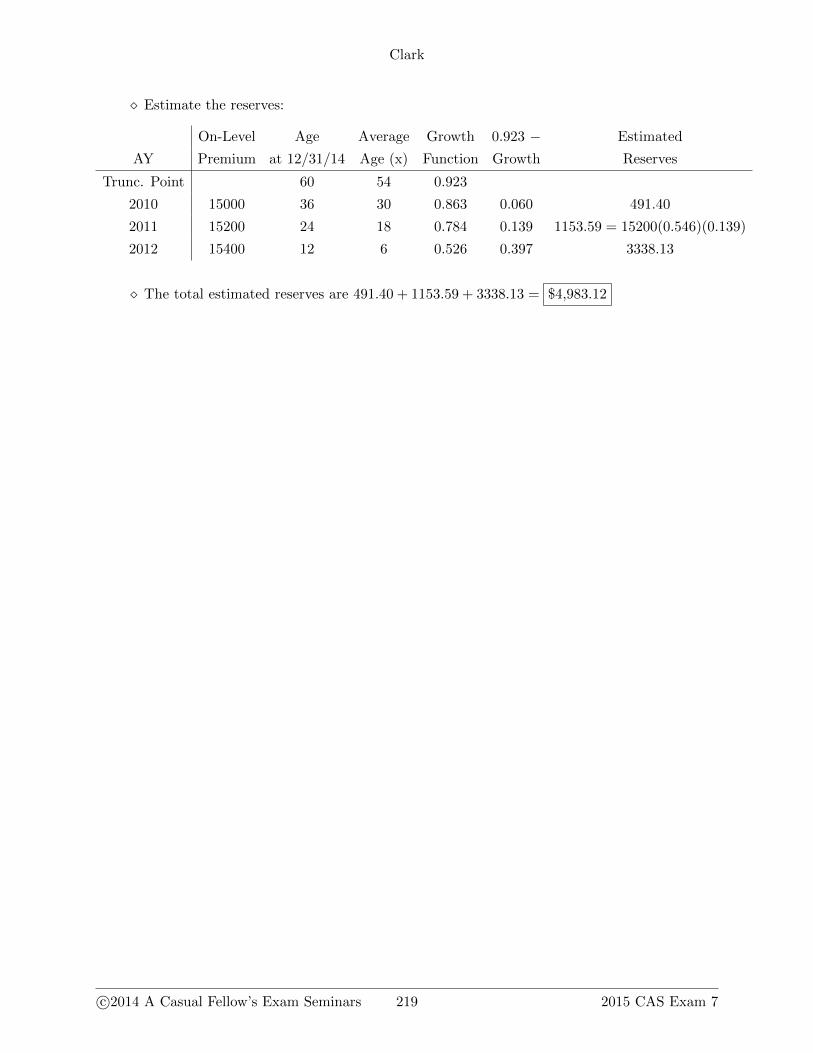
� Estimate the reserves:
On-Level Age Average Growth 0.923 − Estimated
AY Premium at 12/31/14 Age (x) Function Growth Reserves
Trunc. Point 60 54 0.923
2010 15000 36 30 0.863 0.060 491.40
2011 15200 24 18 0.784 0.139 1153.59 = 15200(0.546)(0.139)
2012 15400 12 6 0.526 0.397 3338.13
� The total estimated reserves are 491.40 + 1153.59 + 3338.13 = $4,983.12
c©2014 A Casual Fellow’s Exam Seminars 219 2015 CAS Exam 7

Clark
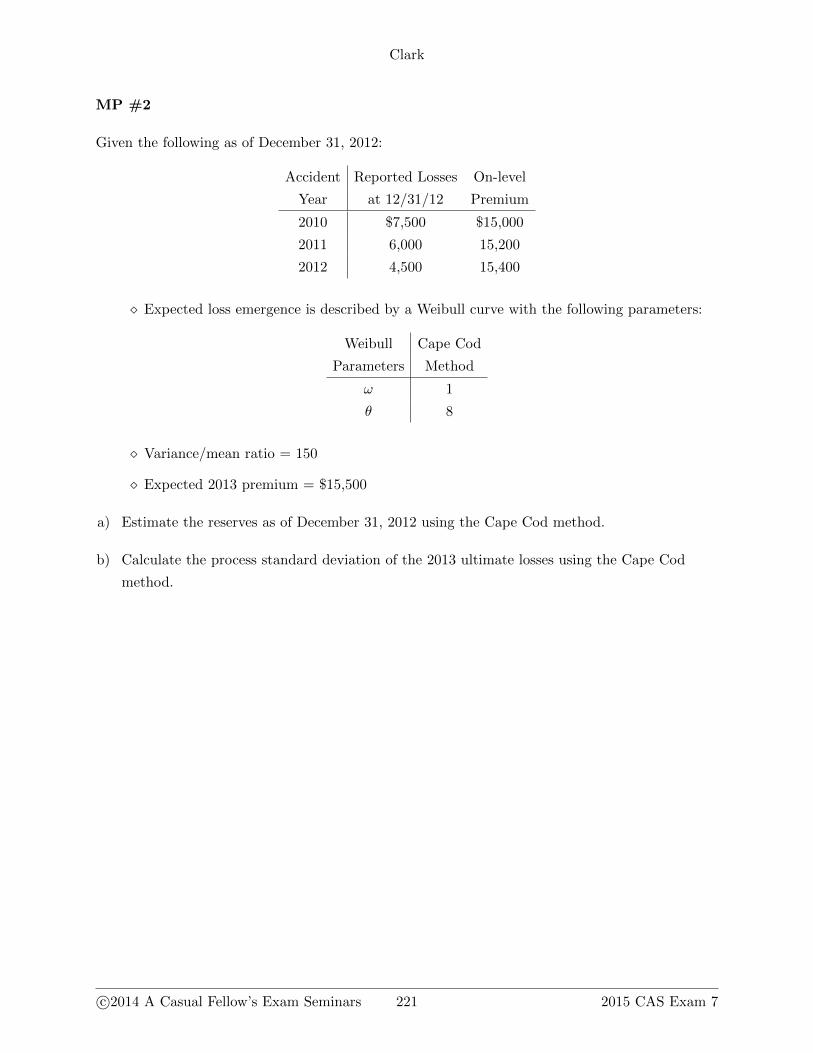
MP #2
Given the following as of December 31, 2012:
Accident Reported Losses On-level
Year at 12/31/12 Premium
2010 $7,500 $15,000
2011 6,000 15,200
2012 4,500 15,400
� Expected loss emergence is described by a Weibull curve with the following parameters:
Weibull Cape Cod
Parameters Method
ω 1
θ 8
� Variance/mean ratio = 150
� Expected 2013 premium = $15,500
a) Estimate the reserves as of December 31, 2012 using the Cape Cod method.
b) Calculate the process standard deviation of the 2013 ultimate losses using the Cape Cod
method.
c©2014 A Casual Fellow’s Exam Seminars 221 2015 CAS Exam 7

Clark
Solution to part a:
� Calculate the expected loss ratio:
On-Level Losses Age Average Growth Premium
AY Premium at 12/31/12 at 12/31/12 Age (x) Function 1 − Growth × Growth
2010 15000 7500 36 30 0.976 0.024 14640
2011 15200 6000 24 18 0.895 0.105 13604
2012 15400 4500 12 6 0.528 0.472 8131.20
• Here are the 2011 calculations for the table above:
� Average age = 18 = 24− 6
� Growth function = 1− exp(−(x/θ)ω) = 1− exp(−(18/8)1) = 0.895
� 1−Growth = 1− 0.895 = 0.105
� Premium× growth = 15200(0.895) = 13604
• The expected loss ratio is 7500+6000+450014640+13604+8131.20 = 0.495
� Estimate the reserves:
AY Premium × ELR 1 − Growth Estimated Reserves
2010 7425 0.024 178.20
2011 7524 = 15200(0.495) 0.105 790.02 = 7524(0.105)
2012 7623 0.472 3598.06
� The total estimated reserves are 178.20 + 790.02 + 3598.06 = $4,566.28
Solution to part b:
� The estimated 2013 ultimate losses are 15500(0.495) = 7672.50
� The process variance for the 2013 ultimate losses is the variance/mean ratio times the
estimated 2013 ultimate losses
� Thus, the process standard deviation of the 2013 ultimate losses is√
150(7672.50) =
$1,072.79
2015 CAS Exam 7 222 c©2014 A Casual Fellow’s Exam Seminars
Clark
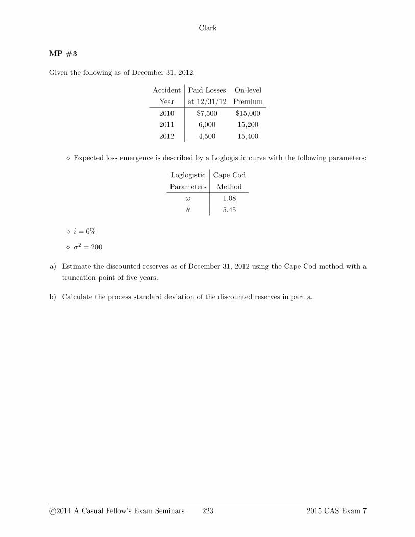
MP #3
Given the following as of December 31, 2012:
Accident Paid Losses On-level
Year at 12/31/12 Premium
2010 $7,500 $15,000
2011 6,000 15,200
2012 4,500 15,400
� Expected loss emergence is described by a Loglogistic curve with the following parameters:
Loglogistic Cape Cod
Parameters Method
ω 1.08
θ 5.45
� i = 6%
� σ2 = 200
a) Estimate the discounted reserves as of December 31, 2012 using the Cape Cod method with a
truncation point of five years.
b) Calculate the process standard deviation of the discounted reserves in part a.
c©2014 A Casual Fellow’s Exam Seminars 223 2015 CAS Exam 7
Clark
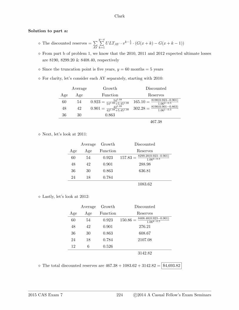
Solution to part a:
� The discounted reserves =∑AY
y−x∑k=1
ULTAY · vk−12 · (G(x+ k)−G(x+ k − 1))
� From part b of problem 1, we know that the 2010, 2011 and 2012 expected ultimate losses
are 8190, 8299.20 & 8408.40, respectively
� Since the truncation point is five years, y = 60 months = 5 years
� For clarity, let’s consider each AY separately, starting with 2010:
Average Growth Discounted
Age Age Function Reserves
60 54 0.923 = 541.08
541.08+5.451.08165.10 = 8190(0.923−0.901)
1.062−0.5
48 42 0.901 = 421.08
421.08+5.451.08302.28 = 8190(0.901−0.863)
1.061−0.5
36 30 0.863
467.38
� Next, let’s look at 2011:
Average Growth Discounted
Age Age Function Reserves
60 54 0.923 157.83 = 8299.20(0.923−0.901)1.063−0.5
48 42 0.901 288.98
36 30 0.863 636.81
24 18 0.784
1083.62
� Lastly, let’s look at 2012:
Average Growth Discounted
Age Age Function Reserves
60 54 0.923 150.86 = 8408.40(0.923−0.901)1.064−0.5
48 42 0.901 276.21
36 30 0.863 608.67
24 18 0.784 2107.08
12 6 0.526
3142.82
� The total discounted reserves are 467.38 + 1083.62 + 3142.82 = $4,693.82
2015 CAS Exam 7 224 c©2014 A Casual Fellow’s Exam Seminars
Clark
Solution to part b:
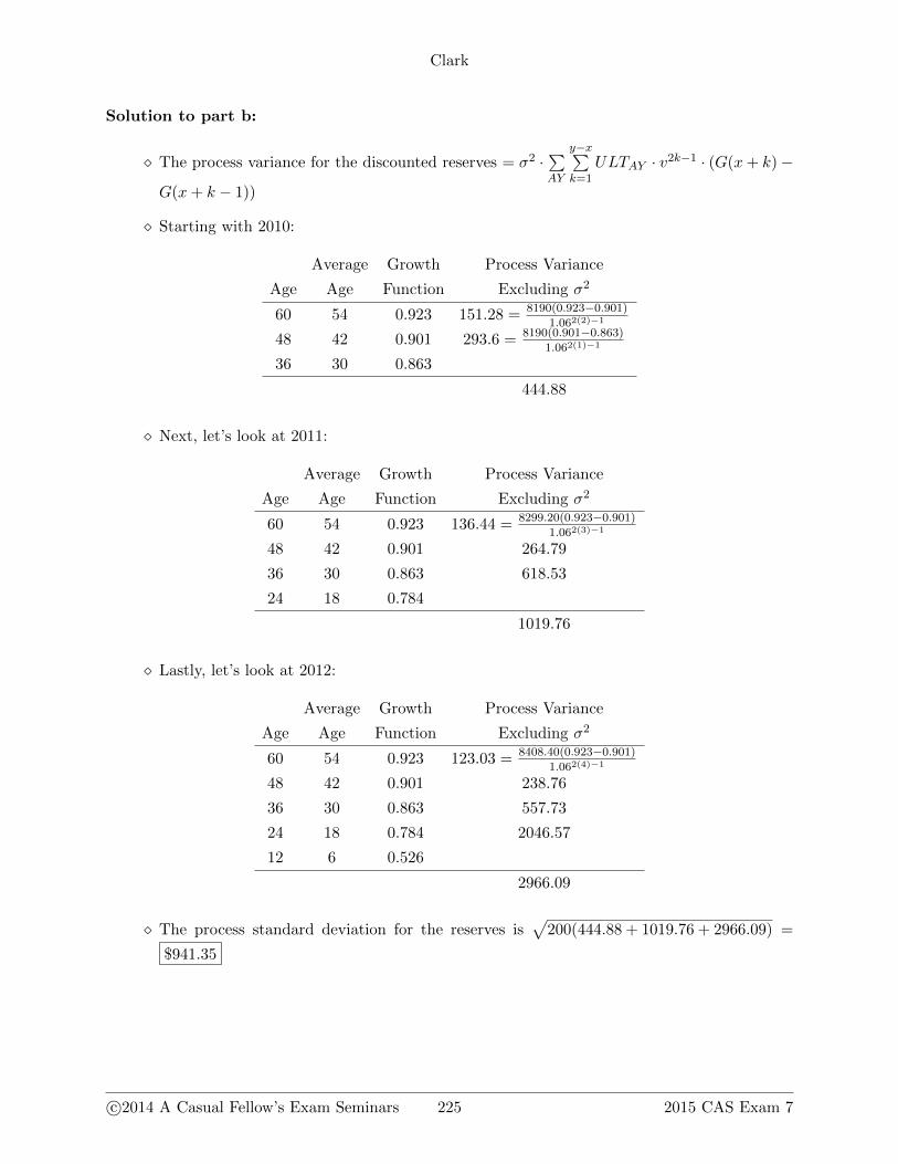
� The process variance for the discounted reserves = σ2 ·∑AY
y−x∑k=1
ULTAY · v2k−1 · (G(x+ k)−
G(x+ k − 1))
� Starting with 2010:
Average Growth Process Variance
Age Age Function Excluding σ2
60 54 0.923 151.28 = 8190(0.923−0.901)
1.062(2)−1
48 42 0.901 293.6 = 8190(0.901−0.863)
1.062(1)−1
36 30 0.863
444.88
� Next, let’s look at 2011:
Average Growth Process Variance
Age Age Function Excluding σ2
60 54 0.923 136.44 = 8299.20(0.923−0.901)
1.062(3)−1
48 42 0.901 264.79
36 30 0.863 618.53
24 18 0.784
1019.76
� Lastly, let’s look at 2012:
Average Growth Process Variance
Age Age Function Excluding σ2
60 54 0.923 123.03 = 8408.40(0.923−0.901)
1.062(4)−1
48 42 0.901 238.76
36 30 0.863 557.73
24 18 0.784 2046.57
12 6 0.526
2966.09
� The process standard deviation for the reserves is√
200(444.88 + 1019.76 + 2966.09) =
$941.35
c©2014 A Casual Fellow’s Exam Seminars 225 2015 CAS Exam 7

Clark
MP #4
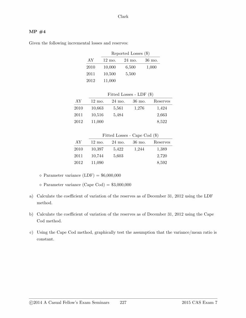
Given the following incremental losses and reserves:
Reported Losses ($)
AY 12 mo. 24 mo. 36 mo.
2010 10,000 6,500 1,000
2011 10,500 5,500
2012 11,000
Fitted Losses - LDF ($)
AY 12 mo. 24 mo. 36 mo. Reserves
2010 10,663 5,561 1,276 1,424
2011 10,516 5,484 2,663
2012 11,000 8,522
Fitted Losses - Cape Cod ($)
AY 12 mo. 24 mo. 36 mo. Reserves
2010 10,397 5,422 1,244 1,389
2011 10,744 5,603 2,720
2012 11,090 8,592
� Parameter variance (LDF) = $6,000,000
� Parameter variance (Cape Cod) = $3,000,000
a) Calculate the coefficient of variation of the reserves as of December 31, 2012 using the LDF
method.
b) Calculate the coefficient of variation of the reserves as of December 31, 2012 using the Cape
Cod method.
c) Using the Cape Cod method, graphically test the assumption that the variance/mean ratio is
constant.
c©2014 A Casual Fellow’s Exam Seminars 227 2015 CAS Exam 7
Clark
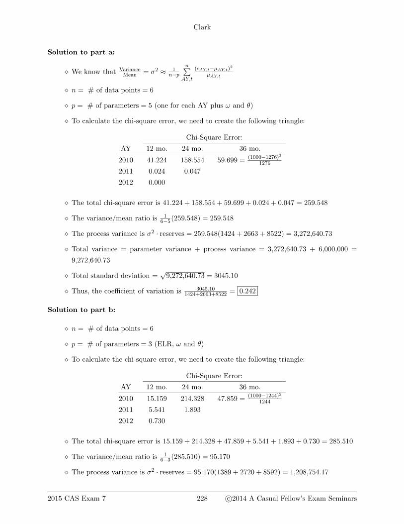
Solution to part a:
� We know that VarianceMean = σ2 ≈ 1
n−p
n∑AY,t
(cAY,t−µAY,t)2µAY,t
� n = # of data points = 6
� p = # of parameters = 5 (one for each AY plus ω and θ)
� To calculate the chi-square error, we need to create the following triangle:
Chi-Square Error:
AY 12 mo. 24 mo. 36 mo.
2010 41.224 158.554 59.699 = (1000−1276)2
1276
2011 0.024 0.047
2012 0.000
� The total chi-square error is 41.224 + 158.554 + 59.699 + 0.024 + 0.047 = 259.548
� The variance/mean ratio is 16−5(259.548) = 259.548
� The process variance is σ2 · reserves = 259.548(1424 + 2663 + 8522) = 3,272,640.73
� Total variance = parameter variance + process variance = 3,272,640.73 + 6,000,000 =
9,272,640.73
� Total standard deviation =√
9,272,640.73 = 3045.10
� Thus, the coefficient of variation is 3045.101424+2663+8522 = 0.242
Solution to part b:
� n = # of data points = 6
� p = # of parameters = 3 (ELR, ω and θ)
� To calculate the chi-square error, we need to create the following triangle:
Chi-Square Error:
AY 12 mo. 24 mo. 36 mo.
2010 15.159 214.328 47.859 = (1000−1244)2
1244
2011 5.541 1.893
2012 0.730
� The total chi-square error is 15.159 + 214.328 + 47.859 + 5.541 + 1.893 + 0.730 = 285.510
� The variance/mean ratio is 16−3(285.510) = 95.170
� The process variance is σ2 · reserves = 95.170(1389 + 2720 + 8592) = 1,208,754.17
2015 CAS Exam 7 228 c©2014 A Casual Fellow’s Exam Seminars

Clark
� Total variance = process variance + parameter variance = 1,208,754.17 + 3,000,000 =
4,208,754.17
� Total standard deviation =√
4,208,754.17 = 2051.52
� Thus, the coefficient of variation is 2051.521389+2720+8592 = 0.162
Solution to part c:
� To test the assumption that the variance/mean ratio is constant, we can graph the normal-
ized residuals against the expected incremental losses
� The normalized residual, rAY ;x,y =cAY ;x,y−µ̂AY ;x,y√
σ2·µ̂AY ;x,y. Using this formula, we can create the
following normalized residual triangle:
Normalized Residuals:
AY 12 mo. 24 mo. 36 mo.
2010 -0.399 1.501 -0.709 = (1000−1244)√95.17(1244)
2011 -0.241 -0.141
2012 -0.088
� We now have the following data pairs:
Expected Normalized
Incremental Loss Residual
1244 -0.709
5422 1.501
5603 -0.141
10397 -0.399
10744 -0.241
11090 -0.088
c©2014 A Casual Fellow’s Exam Seminars 229 2015 CAS Exam 7
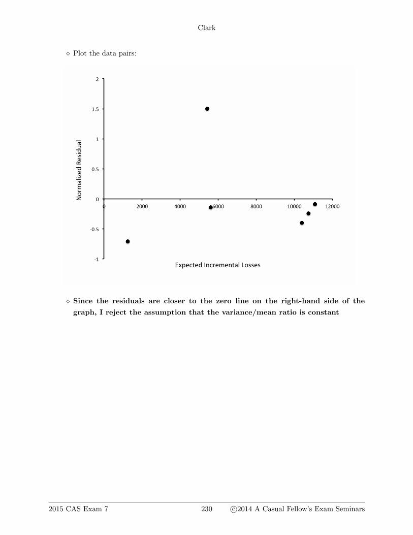
Clark
� Plot the data pairs:
!"#
!$%&#
$#
$%&#
"#
"%&#
'#
$# '$$$# ($$$# )$$$# *$$$# "$$$$# "'$$$#
+,-./0.1#23/4.5.3067#89::.:#
;945
67<=.1#>.:<1?67#
� Since the residuals are closer to the zero line on the right-hand side of the
graph, I reject the assumption that the variance/mean ratio is constant
2015 CAS Exam 7 230 c©2014 A Casual Fellow’s Exam Seminars
Clark
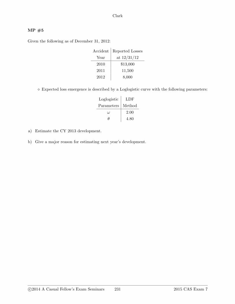
MP #5
Given the following as of December 31, 2012:
Accident Reported Losses
Year at 12/31/12
2010 $13,000
2011 11,500
2012 8,000
� Expected loss emergence is described by a Loglogistic curve with the following parameters:
Loglogistic LDF
Parameters Method
ω 2.00
θ 4.80
a) Estimate the CY 2013 development.
b) Give a major reason for estimating next year’s development.
c©2014 A Casual Fellow’s Exam Seminars 231 2015 CAS Exam 7

Clark
Solution to part a:
� Create the following table:
Losses at Avg. Age at Growth at Avg. Age at Growth at Estimated Estimated
AY 12/31/12 12/31/12 12/31/12 12/31/13 12/31/13 Ultimate CY 2013 Dev.
2010 13000 30 0.975 42 0.987 13333.33 160.00
2011 11500 18 0.934 30 0.975 12312.63 504.82
2012 8000 6 0.610 18 0.934 13114.75 4249.18
• Here are the 2011 calculations for the table above:
� Growth at 12/31/12 = 182
182+4.82= 0.934
� Growth at 12/31/13 = 302
302+4.82= 0.975
� Estimated ultimate = 11500/0.934 = 12312.63
� Estimate CY 2013 development = (0.975− 0.934)(12312.63) = 504.82
� The total CY 2013 development is 160 + 504.82 + 4249.18 = $4,914
Solution to part b:
� A major reason for calculating the CY 2013 development is that the estimate is quickly
testable. One year later, we can compare it to the actual development and see if it was
within the forecast range
2015 CAS Exam 7 232 c©2014 A Casual Fellow’s Exam Seminars
Clark
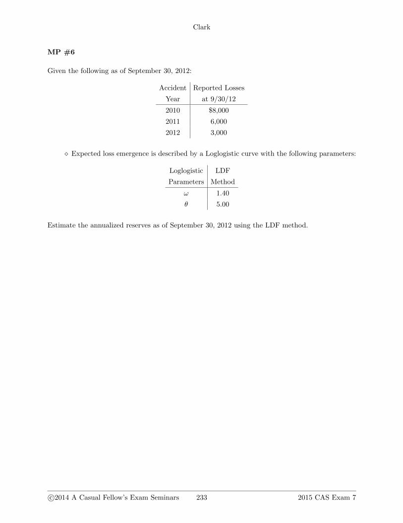
MP #6
Given the following as of September 30, 2012:
Accident Reported Losses
Year at 9/30/12
2010 $8,000
2011 6,000
2012 3,000
� Expected loss emergence is described by a Loglogistic curve with the following parameters:
Loglogistic LDF
Parameters Method
ω 1.40
θ 5.00
Estimate the annualized reserves as of September 30, 2012 using the LDF method.
c©2014 A Casual Fellow’s Exam Seminars 233 2015 CAS Exam 7
Clark
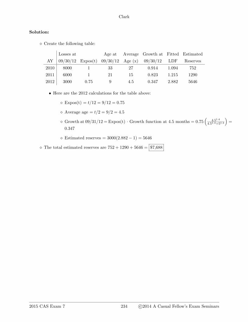
Solution:
� Create the following table:
Losses at Age at Average Growth at Fitted Estimated
AY 09/30/12 Expos(t) 09/30/12 Age (x) 09/30/12 LDF Reserves
2010 8000 1 33 27 0.914 1.094 752
2011 6000 1 21 15 0.823 1.215 1290
2012 3000 0.75 9 4.5 0.347 2.882 5646
• Here are the 2012 calculations for the table above:
� Expos(t) = t/12 = 9/12 = 0.75
� Average age = t/2 = 9/2 = 4.5
� Growth at 09/31/12 = Expos(t) · Growth function at 4.5 months = 0.75(
4.51.4
4.51.4+51.4
)=
0.347
� Estimated reserves = 3000(2.882− 1) = 5646
� The total estimated reserves are 752 + 1290 + 5646 = $7,688
2015 CAS Exam 7 234 c©2014 A Casual Fellow’s Exam Seminars
Clark
Original Essay Problems
EP #1
Provide three advantages of using parameterized curves to describe loss emergence patterns.
EP #2
In a stochastic framework, explain why the Cape Cod method is preferred over the LDF method
when few data points exist.
EP #3
Briefly describe the two components of the variance of the actual loss emergence.
EP #4
Provide two advantages of using the over-dispersed Poisson distribution to model the actual loss
emergence.
EP #5
Fully describe the key assumptions underlying the model outlined in Clark.
EP #6
Briefly describe three graphical tests that can be used to validate Clark’s model assumptions.
EP #7
Briefly explain why it might be necessary to truncate LDFs when using growth curves.
EP #8
Compare and contrast the process and parameter variances of the Cape Cod method and the LDF
method.
EP #9
An actuary used maximum likelihood to parameterize a reserving model. Due to management
discretion, the carried reserves differ from the maximum likelihood estimate.
a) Explain why it may NOT be appropriate to use the coefficient of variation in the model to
describe the carried reserve.
c©2014 A Casual Fellow’s Exam Seminars 235 2015 CAS Exam 7

Clark
b) Explain why it may be appropriate to use the coefficient of variation in the model to describe
the carried reserve.
2015 CAS Exam 7 236 c©2014 A Casual Fellow’s Exam Seminars
Clark
Original Essay Solutions
ES #1
� Estimation is simple since we only have to estimate two parameters
� We can use data from triangles that do NOT have evenly spaced evaluation data
� The final pattern is smooth and does not follow random movements in the historical age-
to-age factors
ES #2
� The Cape Cod method is preferred since it requires the estimation of fewer parameters.
Since the LDF method requires a parameter for each AY, as well as the parameters for the
growth curve, it tends to be over-parameterized when few data points exist
ES #3
� Process variance – the random variation in the actual loss emergence
� Parameter variance – the uncertainty in the estimator
ES #4
� Inclusion of scaling factors allows us to match the first and second moments of any distri-
bution. Thus, there is high flexibility
� Maximum likelihood estimation produces the LDF and Cape Cod estimates of ultimate
losses. Thus, the results can be presented in a familiar format
ES #5
� Assumption 1: Incremental losses are independent and identically distributed (iid)
• “Independence” means that one period does not affect the surrounding periods
• “Identically distributed” assumes that the emergence pattern is the same for all acci-
dent years, which is clearly over-simplified
� Assumption 2: The variance/mean scale parameter σ2 is fixed and known
• Technically, σ2 should be estimated simultaneously with the other model parameters,
with the variance around its estimate included in the covariance matrix. However,
doing so results in messy mathematics. For convenience and simplicity, we assume
that σ2 is fixed and known
c©2014 A Casual Fellow’s Exam Seminars 237 2015 CAS Exam 7
Clark
� Assumption 3: Variance estimates are based on an approximation to the Rao-Cramer lower
bound
• The estimate of variance based on the information matrix is only exact when we are
using linear functions
• Since our model is non-linear, the variance estimate is a Rao-Cramer lower bound (i.e.
the variance estimate is as low as it possibly can be)
ES #6
� Plot the normalized residuals against the following:
• Increment age – if residuals are randomly scattered around zero with a roughly constant
variance, we can assume the growth curve is appropriate
• Expected loss in each increment age – if residuals are randomly scattered around zero
with a roughly constant variance, we can assume the variance/mean ratio is constant
• Calendar year – if residuals are randomly scattered around zero with a roughly constant
variance, we can assume that there are no calendar year effects
ES #7
� For curves with heavy tails (such as loglogistic), it may be necessary to truncate the LDF
at a finite point in time to reduce reliance on the extrapolation
ES #8
� Process variance – the Cape Cod method can produce a higher or lower process variance
than the LDF method
� Parameter variance – the Cape Cod method produces a lower parameter variance than
the LDF method since it requires fewer parameters and incorporates information from the
exposure base
ES #9
Part a:
� Since the standard deviation in the MLE model is directly tied to the maximum likelihood
estimate, it may not appropriate for the carried reserves
2015 CAS Exam 7 238 c©2014 A Casual Fellow’s Exam Seminars

Clark
Part b:
� Since the final carried reserve is a selection based on a number of factors, it stands to reason
that the standard deviation should also be a selection. The output from the MLE model is
a reasonable basis for that selection
c©2014 A Casual Fellow’s Exam Seminars 239 2015 CAS Exam 7


Clark
Past CAS Exam Problems & Solutions
E7 2014 #3
Given the following data for a Cape Cod reserve analysis:
Actual Incremental
Reported Losses ($000)
Accident 12 24 36
Year Months Months Months
2010 100 255 180
2011 120 280
2012 120
Expected Incremental
Reported Losses ($000)
Accident 12 24 36
Year Months Months Months
2010 80 300 200
2011 80 320
2012 100
The parameters of the loglogistic growth curve (ω and θ) and the expected loss ratio (ELR) were
previously estimated, resulting in a total estimated reserve of $1,500,000. The parameter standard
deviation of the total estimated reserve is $350,000.
Calculate the standard deviation of the reserve due to parameter and process variance com-
bined.
c©2014 A Casual Fellow’s Exam Seminars 241 2015 CAS Exam 7
Clark
Solution:
� We know that VarianceMean = σ2 ≈ 1
n−p
n∑AY,t
(cAY,t−µAY,t)2µAY,t
� n = # of data points = 6
� p = # of parameters = 3 (ELR, ω and θ)
� To calculate the chi-square error, we need to create the following triangle:
Chi-Square Error:
AY 12 mo. 24 mo. 36 mo.
2010 5 6.75 2 = (180−200)2
200
2011 20 5
2012 4
� The total chi-square error is 5 + 6.75 + 2 + 20 + 5 + 4 = 42.75
� The variance/mean ratio is 16−3(42.75) = 14.25. Since the numbers in the table above are
in thousands, we convert this to 14250
� The process variance is σ2 · reserves = 14250(1500000)
� Total variance = parameter variance + process variance = 3500002 + 14250(1500000)
� Total standard deviation =√
3500002 + 14250(1500000) = $379,308.58
2015 CAS Exam 7 242 c©2014 A Casual Fellow’s Exam Seminars

Clark
E7 2014 #5
An insurance company has 1,000 exposures uniformly distributed throughout the accident year.
The a priori ultimate loss is $800 per exposure unit.
The expected loss payment pattern is approximated by the following loglogistic function where G
is the cumulative proportion of ultimate losses paid and x represents the average age of reported
losses in months.
� G(x) = xω
xω+θω
� ω = 2.5
� θ = 24
a) Calculate the expected losses paid in the first 36 months after the beginning of the accident
year.
b) Assume the actual cumulative paid losses at 36 months after the beginning of the accident year
are $650,000. Estimate the ultimate loss for the accident year using assumptions based upon
the Cape Cod method.
c) Estimate the ultimate loss for the accident year based on the loglogistic payment model and
the actual payments through 36 months, disregarding the a priori expectation.
d) Calculate a reserve estimate for the accident year by credibility-weighting two estimates of
ultimate loss in parts b. and c. above using the Benktander method.
c©2014 A Casual Fellow’s Exam Seminars 243 2015 CAS Exam 7
Clark
Solution to part a:
� At 36 months after the beginning of the accident year, the average age of the reported losses
is 30 months
� G(30) = 302.5
302.5+242.5= 0.636
� Expected losses = 1000(800)(0.636) = $508,800
Solution to part b:
� Ultimate loss = paid + IBNR = 650000 + 1000(800)(1− 0.636) = $941,200
� Note: I am not a fan of the wording in this part. The problem says “based upon the Cape
Cod method”, but this is more of a BF problem where we use the a priori loss to inform
the IBNR. As an exam taker, use the other parts to help you understand what the CAS is
asking for. In part d., they ask for a Benktander credibility weighting between parts b. and
c. With this in mind, we can deduce that part b. must be asking for a BF ultimate loss
Solution to part c:
� 6500000.636 = $1,022,013
Solution to part d:
� For the Benktander method, Z = pk = G(30) = 0.636
� Ultimate loss = 1022013(0.636) + (1− 0.636)(941200) = 992597
� Reserve = 992597− 650000 = $342,597
2015 CAS Exam 7 244 c©2014 A Casual Fellow’s Exam Seminars
Clark
E7 2013 #3
Given the following information:
Cumulative Paid Loss ($000)
Accident Year 12 24 36
2010 2,750 4,250 5,100
2011 2,700 4,300
2012 2,900
� The expected accident year loss emergence pattern (growth function) is approximated by a
Weibull function of the form:
G(x|ω, θ) = 1− exp(−(x/θ)ω)
� Parameter estimates are: ω = 1.5 and θ = 20
a) Calculate the process standard deviation of the reserve estimate for accident years 2010 through
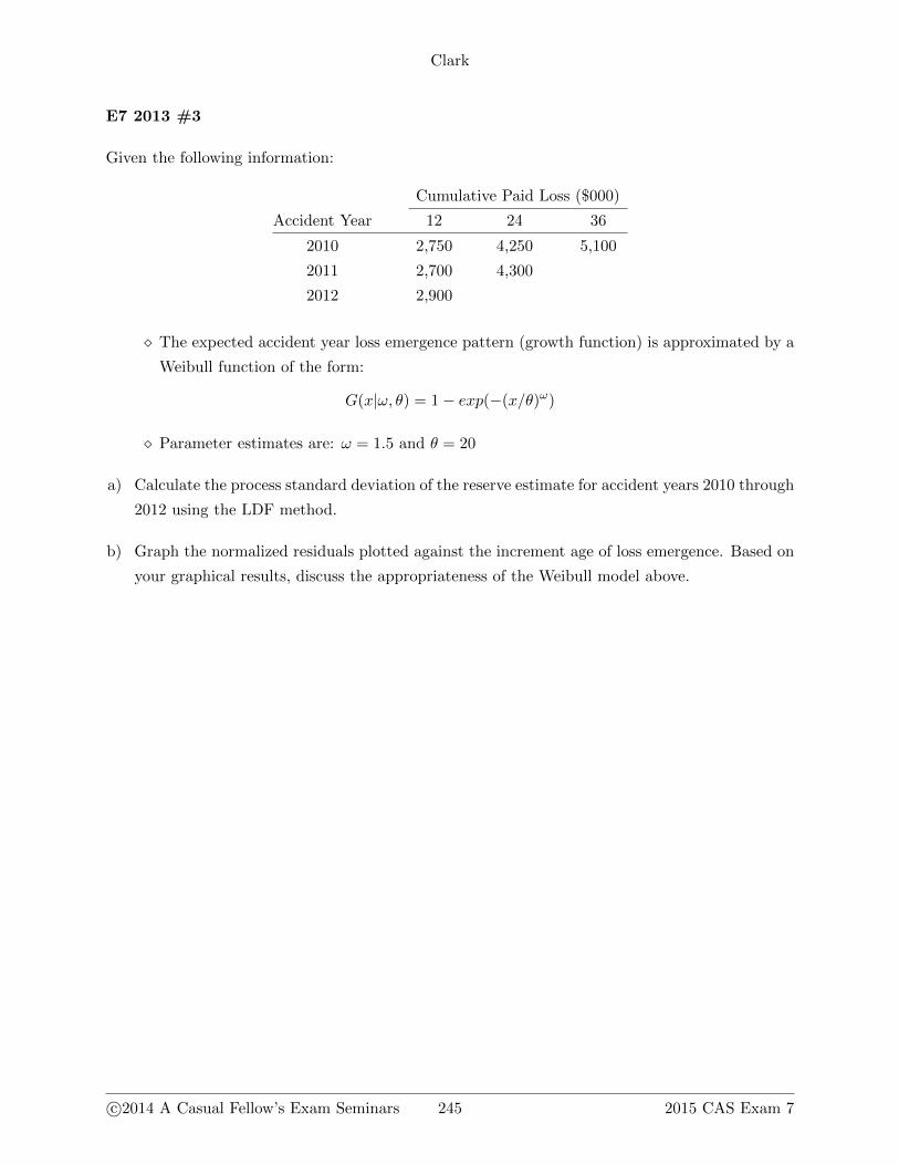
2012 using the LDF method.
b) Graph the normalized residuals plotted against the increment age of loss emergence. Based on
your graphical results, discuss the appropriateness of the Weibull model above.
c©2014 A Casual Fellow’s Exam Seminars 245 2015 CAS Exam 7
Clark
Solution to part a:
� Calculate the reserves
• Create the following table:
Losses Age Average Growth Estimated
AY at 12/31/12 at 12/31/12 Age (x) Function LDF Reserves
2010 5100 36 30 0.841 1.189 963.90
2011 4300 24 18 0.574 1.742 3190.60
2012 2900 12 6 0.152 6.579 16179.10
• Here are the 2011 calculations for the table above:
� Average age = 18 = 24− 6
� Growth function = 1− exp(−(x/θ)ω) = 1− exp(−(18/20)1.5) = 0.574
� LDF = 10.574 = 1.742
� Estimated reserves = 4300(1.742− 1) = 3190.60
• The total estimated reserves are 963.90 + 3190.60 + 16179.10 = 20333.60
� Calculate the process standard deviation
• Create the fitted incremental triangle:
Fitted Incremental Losses:
AY 12 mo. 24 mo. 36 mo.
2010 921.713 = 0.152(5100 + 963.9) 2558.966 1619.061
2011 1138.571 3161.033
2012 2900.023
• Create the chi-square error incremental triangle:
Chi-Square Error:
AY 12 mo. 24 mo. 36 mo.
2010 3626.545 = (2750−921.713)2
921.713 438.227 365.307
2011 2141.334 770.895
2012 0.000
• The total chi-square error is 3626.545 + 438.227 + 365.307 + 2141.334 + 770.895 =
7342.308
• We know that VarianceMean = σ2 ≈ 1
n−p
n∑AY,t
(cAY,t−µAY,t)2µAY,t
2015 CAS Exam 7 246 c©2014 A Casual Fellow’s Exam Seminars
Clark
• n = # of data points = 6
• p = # of parameters = 5 (one for each AY plus ω and θ)
• The variance/mean ratio is 16−5(7342.308) = 7342.308
• The process standard deviation is√σ2 · reserves =
√7342.308(20333.60) = $12,218,656
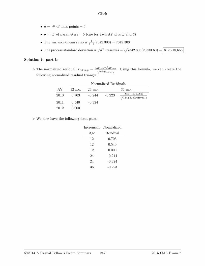
Solution to part b:
� The normalized residual, rAY ;x,y =cAY ;x,y−µ̂AY ;x,y√
σ2·µ̂AY ;x,y. Using this formula, we can create the
following normalized residual triangle:
Normalized Residuals:
AY 12 mo. 24 mo. 36 mo.
2010 0.703 -0.244 -0.223 = (850−1619.061)√7342.308(1619.061)
2011 0.540 -0.324
2012 0.000
� We now have the following data pairs:
Increment Normalized
Age Residual
12 0.703
12 0.540
12 0.000
24 -0.244
24 -0.324
36 -0.223
c©2014 A Casual Fellow’s Exam Seminars 247 2015 CAS Exam 7
Clark
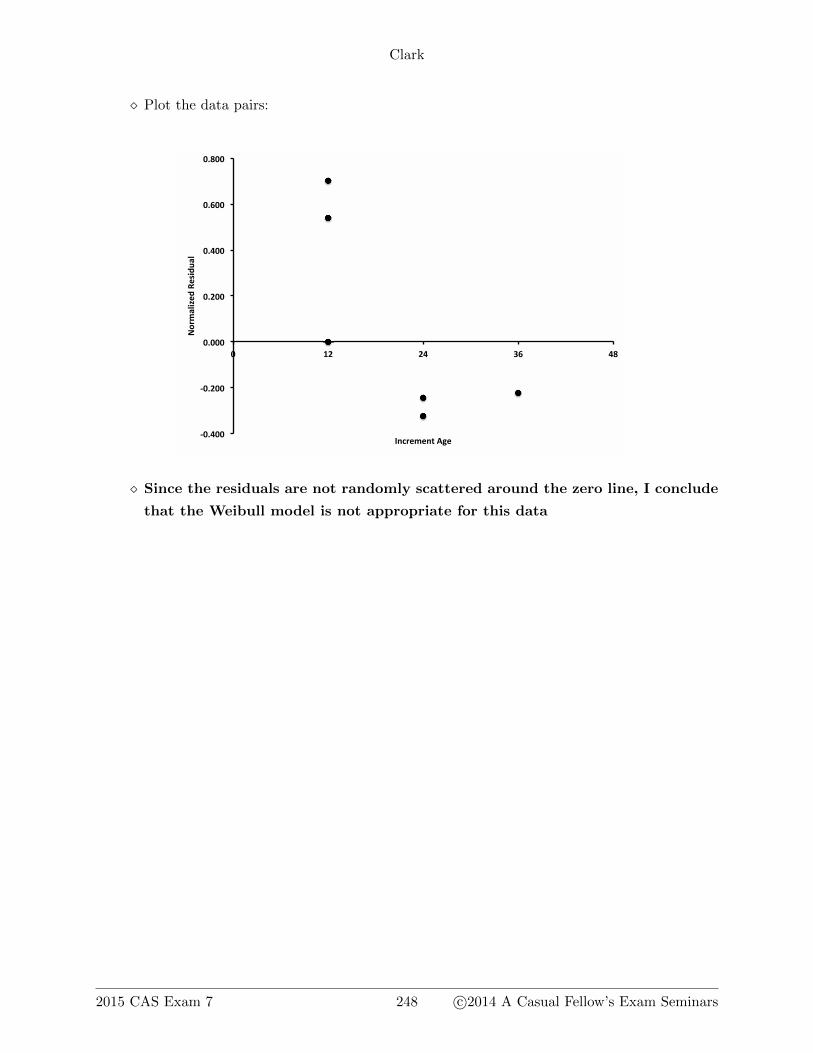
� Plot the data pairs:
!"#$""%
!"#&""%
"#"""%
"#&""%
"#$""%
"#'""%
"#(""%
"% )&% &$% *'% $(%
+,-.
/01234%536147/0%
89:-3.39;%<=3%
� Since the residuals are not randomly scattered around the zero line, I conclude
that the Weibull model is not appropriate for this data
2015 CAS Exam 7 248 c©2014 A Casual Fellow’s Exam Seminars
Clark
E7 2012 #2
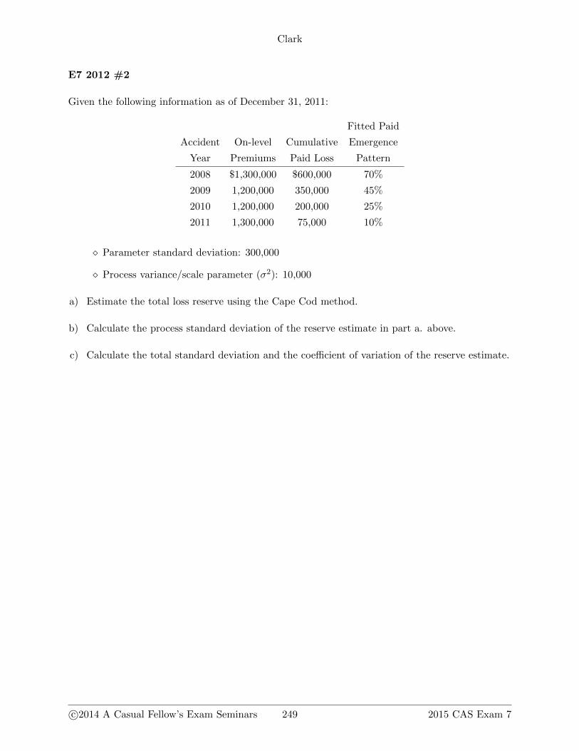
Given the following information as of December 31, 2011:
Fitted Paid
Accident On-level Cumulative Emergence
Year Premiums Paid Loss Pattern
2008 $1,300,000 $600,000 70%
2009 1,200,000 350,000 45%
2010 1,200,000 200,000 25%
2011 1,300,000 75,000 10%
� Parameter standard deviation: 300,000
� Process variance/scale parameter (σ2): 10,000
a) Estimate the total loss reserve using the Cape Cod method.
b) Calculate the process standard deviation of the reserve estimate in part a. above.
c) Calculate the total standard deviation and the coefficient of variation of the reserve estimate.
c©2014 A Casual Fellow’s Exam Seminars 249 2015 CAS Exam 7
Clark
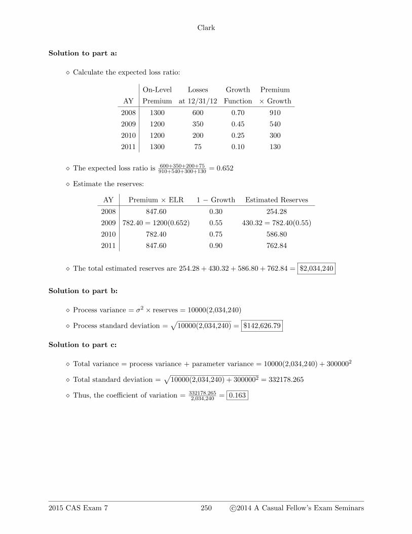
Solution to part a:
� Calculate the expected loss ratio:
On-Level Losses Growth Premium
AY Premium at 12/31/12 Function × Growth
2008 1300 600 0.70 910
2009 1200 350 0.45 540
2010 1200 200 0.25 300
2011 1300 75 0.10 130
� The expected loss ratio is 600+350+200+75910+540+300+130 = 0.652
� Estimate the reserves:
AY Premium × ELR 1 − Growth Estimated Reserves
2008 847.60 0.30 254.28
2009 782.40 = 1200(0.652) 0.55 430.32 = 782.40(0.55)
2010 782.40 0.75 586.80
2011 847.60 0.90 762.84
� The total estimated reserves are 254.28 + 430.32 + 586.80 + 762.84 = $2,034,240
Solution to part b:
� Process variance = σ2 × reserves = 10000(2,034,240)
� Process standard deviation =√
10000(2,034,240) = $142,626.79
Solution to part c:
� Total variance = process variance + parameter variance = 10000(2,034,240) + 3000002
� Total standard deviation =√
10000(2,034,240) + 3000002 = 332178.265
� Thus, the coefficient of variation = 332178.2652,034,240 = 0.163
2015 CAS Exam 7 250 c©2014 A Casual Fellow’s Exam Seminars
Clark
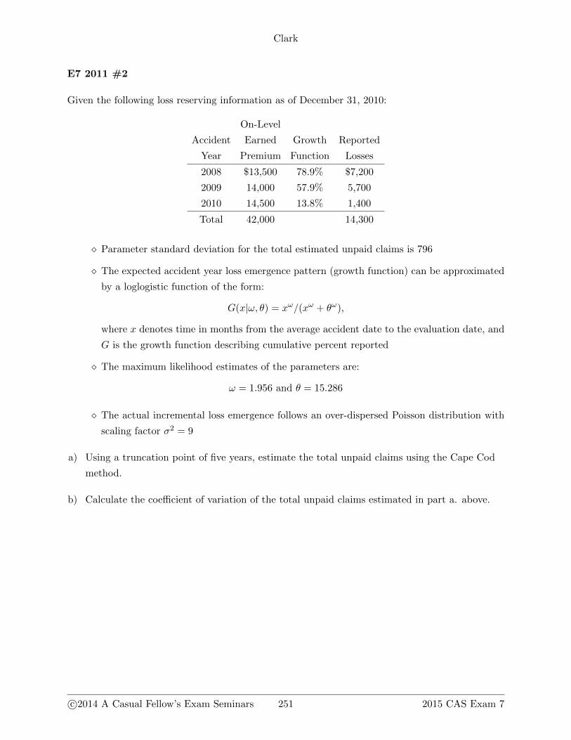
E7 2011 #2
Given the following loss reserving information as of December 31, 2010:
On-Level
Accident Earned Growth Reported
Year Premium Function Losses
2008 $13,500 78.9% $7,200
2009 14,000 57.9% 5,700
2010 14,500 13.8% 1,400
Total 42,000 14,300
� Parameter standard deviation for the total estimated unpaid claims is 796
� The expected accident year loss emergence pattern (growth function) can be approximated
by a loglogistic function of the form:
G(x|ω, θ) = xω/(xω + θω),
where x denotes time in months from the average accident date to the evaluation date, and
G is the growth function describing cumulative percent reported
� The maximum likelihood estimates of the parameters are:
ω = 1.956 and θ = 15.286
� The actual incremental loss emergence follows an over-dispersed Poisson distribution with
scaling factor σ2 = 9
a) Using a truncation point of five years, estimate the total unpaid claims using the Cape Cod
method.
b) Calculate the coefficient of variation of the total unpaid claims estimated in part a. above.
c©2014 A Casual Fellow’s Exam Seminars 251 2015 CAS Exam 7
Clark
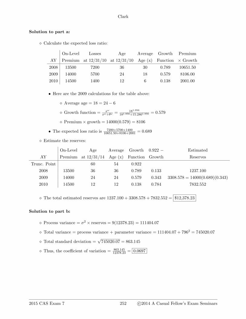
Solution to part a:
� Calculate the expected loss ratio:
On-Level Losses Age Average Growth Premium
AY Premium at 12/31/10 at 12/31/10 Age (x) Function × Growth
2008 13500 7200 36 30 0.789 10651.50
2009 14000 5700 24 18 0.579 8106.00
2010 14500 1400 12 6 0.138 2001.00
• Here are the 2009 calculations for the table above:
� Average age = 18 = 24− 6
� Growth function = xω
xω+θω = 181.956
181.956+15.2861.956= 0.579
� Premium× growth = 14000(0.579) = 8106
• The expected loss ratio is 7200+5700+140010651.50+8106+2001 = 0.689
� Estimate the reserves:
On-Level Age Average Growth 0.922 − Estimated
AY Premium at 12/31/14 Age (x) Function Growth Reserves
Trunc. Point 60 54 0.922
2008 13500 36 36 0.789 0.133 1237.100
2009 14000 24 24 0.579 0.343 3308.578 = 14000(0.689)(0.343)
2010 14500 12 12 0.138 0.784 7832.552
� The total estimated reserves are 1237.100 + 3308.578 + 7832.552 = $12,378.23
Solution to part b:
� Process variance = σ2 × reserves = 9(12378.23) = 111404.07
� Total variance = process variance + parameter variance = 111404.07 + 7962 = 745020.07
� Total standard deviation =√
745020.07 = 863.145
� Thus, the coefficient of variation = 863.14512378.23 = 0.0697
2015 CAS Exam 7 252 c©2014 A Casual Fellow’s Exam Seminars


![Message in a Bottle.1cs229.stanford.edu/proj2017/final-posters/5145028.pdf · binning estimate with a first order correction [2] is unbiased but suffers from large variance. Center:](https://img.pdfslide.net/doc/110x75/5e687851f08186014d5bd90e/message-in-a-bottle-binning-estimate-with-a-first-order-correction-2-is-unbiased.jpg)