Embed Size (px)
Citation preview
Clash of the Titans: MapReduce vs. Spark for Large ScaleData Analytics
Juwei Shi‡, Yunjie Qiu†, Umar Farooq Minhas§, Limei Jiao†, Chen Wang♯, BertholdReinwald§, and Fatma Ozcan§
∗
†IBM Research China §IBM Almaden Research Center‡DEKE, MOE and School of Information, Renmin University of China ♯Tsinghua University
ABSTRACTMapReduce and Spark are two very popular open source clustercomputing frameworks for large scale data analytics. These frame-works hide the complexity of task parallelism and fault-tolerance,by exposing a simple programming API to users. In this paper,we evaluate the major architectural components in MapReduce andSpark frameworks including: shuffle, execution model, and caching,by using a set of important analytic workloads. To conduct a de-tailed analysis, we developed two profiling tools: (1) We corre-late the task execution plan with the resource utilization for bothMapReduce and Spark, and visually present this correlation; (2)We provide a break-down of the task execution time for in-depthanalysis. Through detailed experiments, we quantify the perfor-mance differences between MapReduce and Spark. Furthermore,we attribute these performance differences to different componentswhich are architected differently in the two frameworks. We fur-ther expose the source of these performance differences by usinga set of micro-benchmark experiments. Overall, our experimentsshow that Spark is about 2.5x, 5x, and 5x faster than MapReduce,for Word Count, k-means, and PageRank, respectively. The maincauses of these speedups are the efficiency of the hash-based aggre-gation component for combine, as well as reduced CPU and diskoverheads due to RDD caching in Spark. An exception to this isthe Sort workload, for which MapReduce is 2x faster than Spark.We show that MapReduce’s execution model is more efficient forshuffling data than Spark, thus making Sort run faster on MapRe-duce.
1. INTRODUCTIONIn the past decade, open source analytic software running on
commodity hardware made it easier to run jobs which previouslyused to be complex and tedious to run. Examples include: textanalytics, log analytics, and SQL like query processing, runningat a very large scale. The two most popular open source frame-works for such large scale data processing on commodity hardware
∗This work has been done while Juwei Shi and Chen Wang wereResearch Staff Members at IBM Research-China.
This work is licensed under the Creative Commons AttributionNonCommercialNoDerivs 3.0 Unported License. To view a copy of this license, visit http://creativecommons.org/licenses/byncnd/3.0/. Obtain permission prior to any use beyond those covered by the license. Contactcopyright holder by emailing [email protected]. Articles from this volumewere invited to present their results at the 42nd International Conference onVery Large Data Bases, September 5th September 9th 2016, New Delhi,India.Proceedings of the VLDB Endowment, Vol. 8, No. 13Copyright 2015 VLDB Endowment 21508097/15/09.
are: MapReduce [7] and Spark [19]. These systems provide sim-ple APIs, and hide the complexity of parallel task execution andfault-tolerance from the user.
1.1 Cluster Computing ArchitecturesMapReduce is one of the earliest and best known commodity
cluster frameworks. MapReduce follows the functional program-ming model [8], and performs explicit synchronization across com-putational stages. MapReduce exposes a simple programming APIin terms of map() and reduce() functions. Apache Hadoop [1]is a widely used open source implementation of MapReduce.
The simplicity of MapReduce is attractive for users, but the frame-work has several limitations. Applications such as machine learn-ing and graph analytics iteratively process the data, which meansmultiple rounds of computation are performed on the same data. InMapReduce, every job reads its input data, processes it, and thenwrites it back to HDFS. For the next job to consume the output of apreviously run job, it has to repeat the read, process, and write cy-cle. For iterative algorithms, which want to read once, and iterateover the data many times, the MapReduce model poses a signifi-cant overhead. To overcome the above limitations of MapReduce,Spark [19] uses Resilient Distributed Datasets (RDDs) [19] whichimplement in-memory data structures used to cache intermediatedata across a set of nodes. Since RDDs can be kept in memory,algorithms can iterate over RDD data many times very efficiently.
Although MapReduce is designed for batch jobs, it is widelyused for iterative jobs. On the other hand, Spark has been de-signed mainly for iterative jobs, but it is also used for batch jobs.This is because the new big data architecture brings multiple frame-works together working on the same data, which is already storedin HDFS [17]. We choose to compare these two frameworks dueto their wide spread adoption in big data analytics. All the majorHadoop vendors such as IBM, Cloudera, Hortonworks, and MapRbundle both MapReduce and Spark with their Hadoop distributions.
1.2 Key Architectural ComponentsIn this paper, we conduct a detailed analysis to understand how
Spark and MapReduce process batch and iterative jobs, and whatarchitectural components play a key role for each type of job. Inparticular, we (1) explain the behavior of a set of important ana-lytic workloads which are typically run on MapReduce and Spark,(2) quantify the performance differences between the two frame-works, (3) attribute these performance differences to the differencesin their architectural components.
We identify the following three architectural components andevaluate them through detailed experiments. Studying these com-ponents covers the majority of architectural differences betweenMapReduce and Spark.
2110
Shuffle: The shuffle component is responsible for exchanging in-termediate data between two computational stages 1. For example,in the case of MapReduce, data is shuffled between the map stageand the reduce stage for bulk synchronization. The shuffle compo-nent often affects the scalability of a framework. Very frequently,a sort operation is executed during the shuffle stage. An externalsorting algorithm, such as merge sort, is often required to handlevery large data that does not fit in main memory. Furthermore, ag-gregation and combine are often performed during a shuffle.Execution Model: The execution model component determineshow user defined functions are translated into a physical executionplan. The execution model often affects the resource utilizationfor parallel task execution. In particular, we are interested in (1)parallelism among tasks, (2) overlap of computational stages, and(3) data pipelining among computational stages.Caching: The caching component allows reuse of intermediatedata across multiple stages. Effective caching speeds up iterativealgorithms at the cost of additional space in memory or on disk.In this study, we evaluate the effectiveness of caching availableat different levels including OS buffer cache, HDFS caching [3],Tachyon [11], and RDD caching.
For our experiments, we use five workloads including WordCount, Sort, k-means, linear regression, and PageRank. We choosethese workloads because collectively they cover the important char-acteristics of analytic workloads which are typically run on MapRe-duce and Spark, and they stress the key architectural componentswe are interested in, and hence are important to study. Word Countis used to evaluate the aggregation component because the size ofintermediate data can be significantly reduced by the map side com-biner. Sort is used to evaluate the external sort, data transfer, andthe overlap between map and reduce stages because the size of in-termediate data is large for sort. K-Means and PageRank are usedto evaluate the effectiveness of caching since they are both iterativealgorithms. We believe that the conclusions which we draw fromthese workloads running on MapReduce and Spark can be gener-alized to other workloads with similar characteristics, and thus arevaluable.
1.3 Profiling ToolsTo help us quantify the differences in the above architectural
components between MapReduce and Spark, as well as the behav-ior of a set of important analytic workloads on both frameworks,we developed the following tools for this study.Execution Plan Visualization: To understand a physical exe-cution plan, and the corresponding resource utilization behavior,we correlate the task level execution plan with the resource utiliza-tion, and visually present this correlation, for both MapReduce andSpark.Fine-grained Time Break-down: To understand where time goesfor the key components, we add timers to the Spark source code toprovide the fine-grained execution time break-down. For MapRe-duce, we get this time break-down by extracting this informationfrom the task level logs available in the MapReduce framework.
1.4 ContributionsThe key contributions of this paper are as follows. (1) We con-
duct experiments to thoroughly understand how MapReduce andSpark solve a set of important analytic workloads including bothbatch and iterative jobs. (2) We dissect MapReduce and Sparkframeworks and collect statistics from detailed timers to quantify1For MapReduce, there are two stages: map and reduce. For Spark,there may be many stages, which are built at shuffle dependencies.
differences in their shuffle component. (3) Through a detailed anal-ysis of the execution plan with the corresponding resource utiliza-tion, we attribute performance differences to differences in majorarchitectural components for the two frameworks. (4) We conductmicro-benchmark experiments to further explain non-trivial obser-vations regarding RDD caching.
The rest of the paper is organized as follows. We provide theworkload description in Section 2. In Section 3, we present ourexperimental results along with a detailed analysis. Finally, wepresent a discussion and summary of our findings in Section 4.
2. WORKLOAD DESCRIPTIONIn this section, we identify a set of important analytic workloads
including Word Count (WC), Sort, k-means, linear regression (LR),and PageRank.
Table 1: Characteristics of Selected WorkloadsWordCount
Sort K-Means(LR)
Page-Rank
TypeOne Pass
√ √
Iterative√ √
Shuffle Sel.High
√
Medium√
Low√ √
Job/Iter. Sel.High
√
Medium√
Low√ √
As shown in Table 1, the selected workloads collectively coverthe characteristics of typical batch and iterative analytic applica-tions run on MapReduce and Spark. We evaluate both one-passand iterative jobs. For each type of job, we cover different shuf-fle selectivity (i.e., the ratio of the map output size to the job inputsize, which represents the amount of disk and network I/O for ashuffle), job selectivity (i.e., the ratio of the reduce output size tothe job input size, which represents the amount of HDFS writes),and iteration selectivity (i.e., the ratio of the output size to the inputsize for each iteration, which represents the amount of intermedi-ate data exchanged across iterations). For each workload, giventhe I/O behavior represented by these selectivities, we evaluate itssystem behavior (e.g., CPU-bound, disk-bound, network-bound) tofurther identify the architectural differences between MapReduceand Spark.
Furthermore, we use these workloads to quantitatively evalu-ate different aspects of key architectural components including (1)shuffle, (2) execution model, and (3) caching. As shown in Table 2,for the shuffle component, we evaluate the aggregation framework,external sort, and transfers of intermediate data. For the execu-tion model component, we evaluate how user defined functions aretranslated into to a physical execution plan, with a focus on taskparallelism, stage overlap, and data pipelining. For the cachingcomponent, we evaluate the effectiveness of caching available atdifferent levels for caching both input and intermediate data. Asexplained in Section 1.2, the selected workloads collectively coverall the characteristics required to evaluate these three components.
3. EXPERIMENTS
3.1 Experimental Setup
3.1.1 Hardware ConfigurationOur Spark and MapReduce clusters are deployed on the same
hardware, with a total of four servers. Each node has 32 CPU coresat 2.9 GHz, 9 disk drives at 7.2k RPM with 1 TB each, and 190
2111
Metric Selection
CPU_SYSTEM
CPU_USER
CPU_WIO
MEM_CACHED
MEM_TOTAL
MEM_USED
BYTES_IN
BYTES_OUT
sdb_READ
sdb_WRITE
sdc_READ
sdc_WRITE
sdb_
sdc_
0 20 40 60 80 100 120 140Time (sec)
0 20 40 60 80 100 120 140
Time (sec)20406080100
(%) CPU
0%
0 20 40 60 80 100 120 140
Time (sec)4080120160200
(GB) MEMORY
0 20 40 60 80 100 120 140
Time (sec)20406080100
(MB/s) NETWORK
0 20 40 60 80 100 120 140
Time (sec)20406080100
(MB/s) DISK_IO
0 20 40 60 80 100 120 140
Time (sec)20406080100
(%) DISK_USAGE
(a) MapReduce
Metric Selection
CPU_SYSTEM
CPU_USER
CPU_WIO
MEM_CACHED
MEM_TOTAL
MEM_USED
BYTES_IN
BYTES_OUT
sdb_READ
sdb_WRITE
sdc_READ
sdc_WRITE
sdb_
sdc_
0 5 10 15 20 25 30 35 40 45Time (sec)
0 5 10 15 20 25 30 35 40 45
Time (sec)20406080100
(%) CPU
9%
0 5 10 15 20 25 30 35 40 45
Time (sec)4080120160200
(GB) MEMORY
0 5 10 15 20 25 30 35 40 45
Time (sec)20406080100
(MB/s) NETWORK
0 5 10 15 20 25 30 35 40 45
Time (sec)20406080100
(MB/s) DISK_IO
0 5 10 15 20 25 30 35 40 45
Time (sec)20406080100
(%) DISK_USAGE
(b) Spark
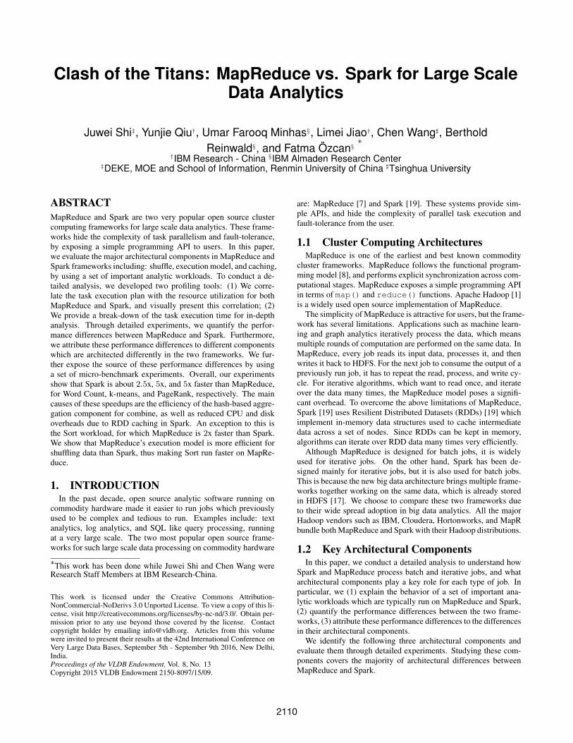
Figure 1: The Execution Details of Word Count (40 GB)
Table 2: Key Architectural Components of InterestWordCount
Sort K-Means(LR)
Page-Rank
ShuffleAggregation
√ √ √
External sort√
Data transfer√ √
ExecutionTask parallelism
√ √ √ √
Stage overlap√
Data pipelining√
CachingInput
√ √
Intermediate data√
GB of physical memory. In aggregate, our four node cluster has128 CPU cores, 760 GB RAM, and 36 TB locally attached storage.The hard disks deliver an aggregate bandwidth of about 125 GB/secfor reads and 45 GB/sec for writes across all nodes, as measuredusing dd. Nodes are connected using a 1 Gbps Ethernet switch.Each node runs 64-bit Red Hat Enterprise Linux 6.4 (kernel version2.6.32).
As a comparison, hardware specifications of our physical clusterare roughly equivalent to a cluster with about 100 virtual machines(VMs) (e.g., m3.medium on AWS2). Our hardware setup is suitablefor evaluating various scalability bottlenecks in Spark and MapRe-duce frameworks. For example, we have enough physical cores inthe system to run many concurrent tasks and thus expose any syn-chronization overheads. However, experiments which may need alarge number of servers (e.g., evaluating the scalability of masternodes) are out of the scope of this paper.
3.1.2 Software ConfigurationBoth MapReduce and Spark are deployed on Java 1.7.0.
Hadoop: We use Hadoop version 2.4.0 to run MapReduce onYARN [17]. We use 8 disks to store intermediate data for MapRe-duce and for storing HDFS data as well. We configure HDFS with128 MB block size and a replication factor of 3. We configureHadoop to run 32 containers per node (i.e., one per CPU core). Tobetter control the degree of parallelism for jobs, we enable CGroupsin YARN and also enable CPU-Scheduling 3. The default JVMheap size is set to 3 GB per task. We tune the following parametersto optimize performance: (1) We use Snappy compression for map
2http://aws.amazon.com/ec2/instance-types/3https://www.kernel.org/doc/Documentation/cgroups/cgroups.txt
output; (2) For all workloads except Sort, we disable the overlapbetween map and reduce stages. This overlap hides the networkoverhead by overlapping computation and network transfer. But itcomes at a cost of reduction in map parallelism, and the networkoverhead is not a bottleneck for any workload except Sort; (3) ForSort, we set the number of reduce tasks to 60 to overlap the shufflestage (network-bound) with the map stage (without network over-head), and for other workloads, we set the number of reduce tasksto 120; (4) We set the number of parallel copiers per task to 2 toreduce the context switching overhead [16]; (5) We set the mapoutput buffer to 550 MB to avoid additional spills for sorting themap output; (6) For Sort, we set the reduce input buffer to 75% ofthe JVM heap size to reduce the disk overhead caused by spills.
Spark: We use Spark version 1.3.0 running in the standalonemode on HDFS 2.4.0. We also use 8 disks for storing Spark in-termediate data. For each node, we run 8 Spark workers whereeach worker is configured with 4 threads (i.e., one thread per CPUcore). We also tested other configurations. We found that when werun 1 worker with 32 threads, the CPU utilization is significantlyreduced. For example, under this configuration, the CPU utilizationdecreases to 33% and 25%, for Word Count and the first iteration ofk-means, respectively. This may be caused by the synchronizationoverhead of memory allocation for multi-threaded tasks. However,CPU can be 100% utilized for all the CPU-bound workloads whenusing 8 workers with 4 threads each. Thus, we use this setting forour experiments. We set the JVM heap size to 16 GB for both theSpark driver and the executors. Furthermore, we tune the followingparameters for Spark: (1) We use Snappy to compress the interme-diate results during a shuffle; (2) For Sort with 500 GB input, we setthe number of tasks for shuffle reads to 2000. For other workloads,this parameter is set to 120.
3.1.3 Profiling toolsIn this section, we present the visualization and profiling tools
which we have developed to perform an in-depth analysis of theselected workloads running on Spark and MapReduce.
Execution Plan Visualization: To understand parallel executionbehavior, we visualize task level execution plans for both MapRe-duce and Spark. First, we extract the execution time of tasks fromjob history of MapReduce and Spark. In order to create a compactview to show parallelism among tasks, we group tasks to horizontal
2112

Table 3: Overall Results: Word CountPlatform Spark MR Spark MR Spark MRInput size (GB) 1 1 40 40 200 200Number of map tasks 9 9 360 360 1800 1800Number of reduce tasks 8 8 120 120 120 120Job time (Sec) 30 64 70 180 232 630Median time of map tasks (Sec) 6 34 9 40 9 40Median time of reduce tasks (Sec) 4 4 8 15 33 50Map Output on disk (GB) 0.03 0.015 1.15 0.7 5.8 3.5
lines. We deploy Ganglia [13] over the cluster, and persist Round-Robin Database [5] to MySQL database periodically. Finally, wecorrelate the system resource utilization (CPU, memory, disk, andnetwork) with the execution plan of tasks using a time line view.
Figure 1 is an example of such an execution plan visualization.At the very top, we present a visualization of the physical execu-tion plan where each task is represented as an horizontal line. Thelength of this line is proportional to the actual execution time of atask. Tasks belonging to different stages are represented in differ-ent colors. The physical execution plan can then be visually corre-lated with the CPU, memory, network, and disk resources, whichare also presented in Figure 1. In the resource utilization graphs,x-axis presents the elapsed time in seconds, and is correlated withthe horizontal axis of the physical execution plan. Moreover, webreak down reduce tasks for MapReduce to three sub-stages: copy,sort, and reduce. For each batch of simultaneously running task(i.e., wave), we can read directly down to correlate resources withthe processing that occurs during that wave.
This tool can show: (1) parallelism of tasks (i.e., waves), e.g.,the first wave is marked in Figure 1 (a), (2) the overlap of stages,e.g., the overlap between map and reduce stages is shown in Fig-ure 2 (b), (3) skewness of tasks, e.g., the skewness of map tasksis shown in Figure 3 (b), and (4) the resource usage behavior foreach stage, e.g., we can see that the map stage is CPU-bound inFigure 3 (a). Note that the goal of our visualization tool is to helpa user analyze details of the physical execution plan, and the corre-sponding resource utilization, in order to gain deeper insights intoa workload’s behavior.
Fine-grained Time Break-down: To understand where time goesfor the shuffle component, we provide the fine-grained executiontime break-down for selected tasks. For Spark, we use System.na-noTime() to add timers to each sub-stage, and aggregate the timeafter a task finishes. In particular, we add timers to the followingcomponents: (1) compute() method for RDD transformation, (2)ShuffleWriter for combine, and (3) BlockObjectWriter forserialization, compression, and shuffle writes. For MapReduce, weuse the task logs to provide the execution time break-down. We findthat such detailed break-downs are sufficient to quantify differencesin the shuffle components of MapReduce and Spark.
3.2 Word CountWe use Word Count (WC) to evaluate the aggregation compo-
nent for both MapReduce and Spark. For these experiments, weuse the example WC program included with both MapReduce andSpark, and we use Hadoop’s random text writer to generate input.
3.2.1 Overall ResultTable 3 presents the overall results for WC for various input
sizes, for both Spark and MapReduce. Spark is about 2.1x, 2.6x,and 2.7x faster than MapReduce for 1 GB, 40 GB, and 200 GBinput, respectively.
Interestingly, Spark is about 3x faster than MapReduce in themap stage. For both frameworks, the application logic and the
Table 4: Time Break-down of Map Tasks for Word CountPlatform Load
(sec)Read(sec)
Map(sec)
Combine(sec)
Serialization(sec)
Compression&write (sec)
Spark 0.1 2.6 1.8 2.3 2.6 0.1MapReduce 6.2 12.6 14.3 5.0
amount of intermediate data is similar. We believe that this dif-ference is due to the differences in the aggregation component. Weevaluate this observation further in Section 3.2.3 below.
For the reduce stage, the execution time is very similar in Sparkand MapReduce because the reduce stage is network-bound and theamount of data to shuffle is similar in both cases.
3.2.2 Execution DetailsFigure 1 shows the detailed execution plan for WC with 40 GB
input. Our deployment of both MapReduce and Spark can exe-cute 128 tasks in parallel, and each task processes 128 MB of data.Therefore, it takes three waves of map tasks (shown in blue in Fig-ure 1) to process the 40 GB input. As we show the execution timewhen the first task starts on the cluster, there may be some initial-ization lag on worker nodes (e.g., 0 to 4 seconds in Figure 1 (b)).Map Stage: We observe that in Spark, the map stage is disk-boundwhile in MapReduce it is CPU-bound. As each task processes thesame amount of data (i.e., 128 MB), this indicates that Spark takesless CPU time than MapReduce in the map stage. This is consistentwith the 3x speed-up shown in Table 3.Reduce Stage: The network resource utilization in Figure 1 showsthat the reduce stage is network-bound for both Spark and MapRe-duce. However, the reduce stage is not a bottleneck for WC because(1) most of the computation is done during the map side combine,and (2) the shuffle selectivity is low (< 2%), which means thatreduce tasks have less data to process.
3.2.3 Breakdown for the Map StageIn order to explain the 3x performance difference during the map
stage, we present the execution time break-down for map tasks inboth Spark and MapReduce in Table 4. The reported executiontimes are an average over 360 map tasks with 40 GB input to WC.First, MapReduce is much slower than Spark in task initialization.Second, Spark is about 2.9x faster than MapReduce in input readand map operations. Last, Spark is about 6.2x faster than MapRe-duce in the combine stage. This is because the hash-based combineis more efficient than the sort-based combine for WC. Spark haslower complexity in its in-memory collection and combine compo-nents, and thus is faster than MapReduce.
3.2.4 Summary of InsightsFor WC and similar workloads such as descriptive statistics, the
shuffle selectivity can be significantly reduced by using a map sidecombiner. For this type of workloads, hash-based aggregation inSpark is more efficient than sort-based aggregation in MapReducedue to the complexity differences in its in-memory collection andcombine components.
3.3 SortFor experiments with Sort, we use TeraSort [15] for MapRe-
duce, and implement Sort using sortByKey() for Spark. Weuse gensort 4 to generate the input for both.
We use experiments with Sort to analyze the architecture of theshuffle component in MapReduce and Spark. The shuffle compo-nent is used by Sort to get a total order on the input and is a bottle-neck for this workload.4http://www.ordinal.com/gensort.html
2113

Metric Selection
CPU_SYSTEM
CPU_USER
CPU_WIO
MEM_CACHED
MEM_TOTAL
MEM_USED
BYTES_IN
BYTES_OUT
sdb_READ
sdb_WRITE
sdc_READ
sdc_WRITE
sdb_
sdc_
0 20 40 60 80 100 120 140 160 180Time (sec)
0 20 40 60 80 100 120 140 160 180
Time (sec)20406080100
(%) CPU
0 20 40 60 80 100 120 140 160 180
Time (sec)4080120160200
(GB) MEMORY
0 20 40 60 80 100 120 140 160 180
Time (sec)20406080100
(MB/s) NETWORK
0 20 40 60 80 100 120 140 160 180
Time (sec)20406080100
(MB/s) DISK_IO
0 20 40 60 80 100 120 140 160 180
Time (sec)20406080100
(%) DISK_USAGE
(a) MapReduce
Metric Selection
CPU_SYSTEM
CPU_USER
CPU_WIO
MEM_CACHED
MEM_TOTAL
MEM_USED
BYTES_IN
BYTES_OUT
sdb_READ
sdb_WRITE
sdc_READ
sdc_WRITE
sdb_
sdc_
0 30 60 90 120 150 180 210 240 270Time (sec)
0 30 60 90 120 150 180 210 240 270
Time (sec)20406080100
(%) CPU
0 30 60 90 120 150 180 210 240 270
Time (sec)4080120160200
(GB) MEMORY
0 30 60 90 120 150 180 210 240 270
Time (sec)20406080100
(MB/s) NETWORK
0 30 60 90 120 150 180 210 240 270
Time (sec)20406080100
(MB/s) DISK_IO
0 30 60 90 120 150 180 210 240 270
Time (sec)20406080100
(%) DISK_USAGE
(b) Spark
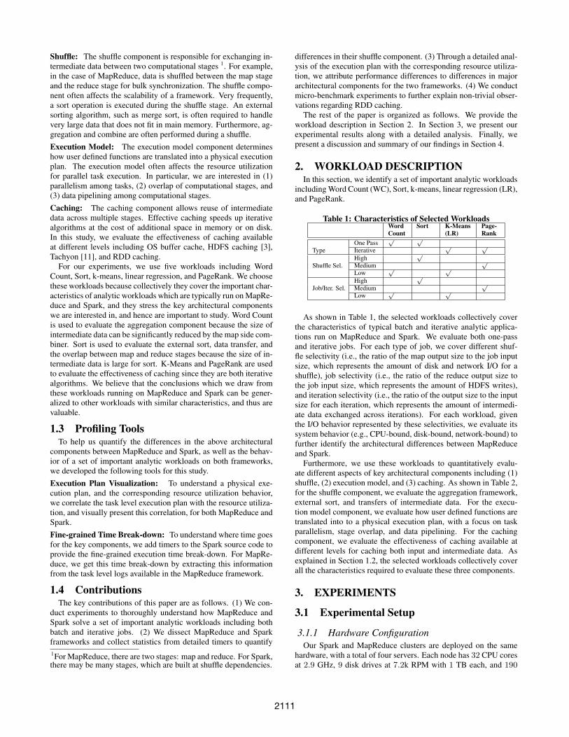
Figure 2: The Execution Details of Sort (100 GB Input)
Table 5: Overall Results: Sort
Platform Spark MR Spark MR Spark MRInput size (GB) 1 1 100 100 500 500Number of map tasks 9 9 745 745 4000 4000Number of reduce tasks 8 8 248 60 2000 60Job time 32s 35s 4.8m 3.3m 44m 24mSampling stage time 3s 1s 1.1m 1s 5.2m 1sMap stage time 7s 11s 1.0m 2.5m 12m 13.9mReduce stage time 11s 24s 2.5m 45s 26m 9.2mMap output on disk (GB) 0.63 0.44 62.9 41.3 317.0 227.2
3.3.1 Overall ResultTable 5 presents the overall results for Sort for 1 GB, 100 GB,
and 500 GB input, for both Spark and MapReduce. For 1 GB input,Spark is faster than MapReduce because Spark has lower controloverhead (e.g., task load time) than MapReduce. MapReduce is1.5x and 1.8x faster than Spark for 100 GB and 500 GB inputs,respectively. Note that the results presented in [6] show that Sparkoutperformed MapReduce in the Daytona Gray Sort benchmark.This difference is mainly because our cluster is connected using 1Gbps Ethernet, as compared to a 10 Gbps Ethernet in [6], i.e., inour cluster configuration network can become a bottleneck for Sortin Spark, as explained in Section 3.3.2 below.
From Table 5 we can see that for the sampling stage, MapReduceis much faster than Spark because of the following reason: MapRe-duce reads a small portion of the input file (100, 000 records from10 selected splits), while Spark scans the whole file. For the mapstage, Spark is 2.5x and 1.2x faster than MapReduce for 100 GBand 500 GB input, respectively. For the reduce stage, MapReduceis 3.3x and 2.8x faster than Spark for 100 GB and 500 GB input,respectively. To better explain this difference, we present a detailedanalysis of the execution plan in Section 3.3.2 and a break-down ofthe execution time in Section 3.3.3 below.
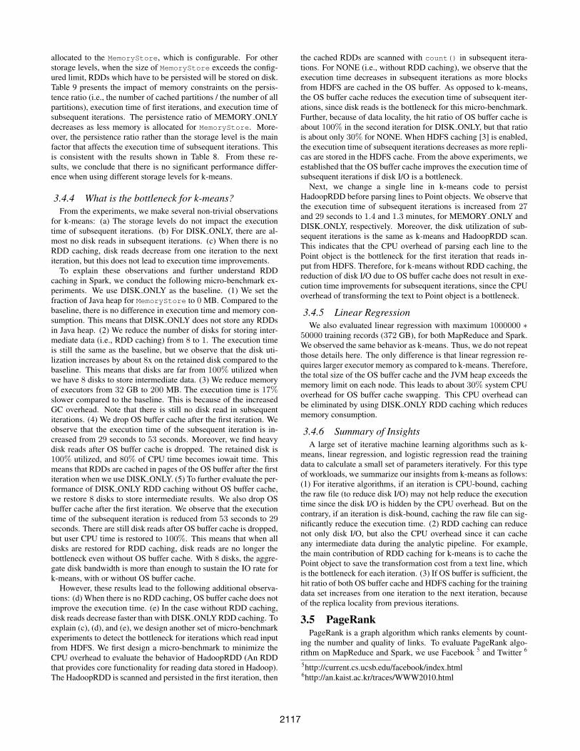
3.3.2 Execution DetailsFigure 2 shows the detailed execution plan of 100 GB Sort for
MapReduce and Spark along with the resource utilization graphs.
Sampling Stage: The sampling stage of MapReduce is performedby a lightweight central program in less than 1 second, so it is notshown in the execution plan. Figure 2 (b) shows that during theinitial part of execution (i.e., sampling stage) in Spark, the diskutilization is quite high while the CPU utilization is low. As we
Table 6: Time Break-down of Map Tasks for SortPlatform Load
(sec)Read(sec)
Map(sec)
Combine(sec)
Serialization(sec)
Compression&write (sec)
Spark-Hash 0.1 1.1 0.8 - 3.0 5.5Spark-Sort 0.1 1.2 0.6 6.4 2.3 2.4MapReduce 6.6 10.5 4.1 2.0
mentioned earlier, Spark scans the whole input file during samplingand is therefore disk-bound.Map Stage: As shown in Figure 2, both Spark and MapReduce areCPU-bound in the map stage. Note that the second stage is the mapstage for Spark. Even though Spark and MapReduce use differentshuffle frameworks, their map stages are bounded by map outputcompression. Furthermore, for Spark, we observe that disk I/O issignificantly reduced in the map stage compared to the samplingstage, although its map stage also scans the whole input file. Thereduced disk I/O is a result of reading input file blocks cached inthe OS buffer during the sampling stage.Reduce Stage: The reduce stage in both Spark and MapReduceuses external sort to get a total ordering on the shuffled map output.MapReduce is 2.8x faster than Spark for this stage. As the execu-tion plan for MapReduce in Figure 2 (a) shows, the main cause ofthis speed-up is that the shuffle stage is overlapped with the mapstage, which hides the network overhead. The current implemen-tation of Spark does not support the overlap between shuffle writeand read stages. This is a notable architectural difference betweenMapReduce and Spark. Spark may want to support this overlap inthe future to improve performance. Last, note that the number ofreplicas in this experiment is set to 1 according to the sort bench-mark [15], thus there is no network overhead for HDFS writes inreduce tasks.
When the input size increases from 100 GB to 500 GB, duringthe map stage in Spark, there is significant CPU overhead for swap-ping pages in OS buffer cache. However, for MapReduce, we ob-serve much less system CPU overhead during the map stage. Thisis the main reason that the map stage speed-up between Spark andMapReduce is reduced from 2.5x to 1.2x.
3.3.3 Breakdown for the Map StageTable 6 shows a break-down of the map task execution time for
both MapReduce and Spark, with 100 GB input. A total of 745map tasks are executed, and we present the average execution time.
2114
We find that there are two stages where MapReduce is slower thanSpark. First, the load time in MapReduce is much slower than thatin Spark. Second, the total times of (1) reading the input (Read),and (2) for applying the map function on the input (Map), is higherthan Spark. The reasons why Spark performs better include: (1)Spark reads part of the input from the OS buffer cache since its sam-pling stage scans the whole input file. On the other hand, MapRe-duce only partially reads the input file during sampling thus OSbuffer cache is not very effective during the map stage. (2) MapRe-duce collects the map output in a map side buffer before flushingit to disk, but Spark’s hash-based shuffle writer, writes each mapoutput record directly to disk, which reduces latency.
3.3.4 Comparison of Shuffle ComponentsSince Sort is dominated by the shuffle stage, we evaluate differ-
ent shuffle frameworks including hash-based shuffle (Spark-Hash),sort-based shuffle (Spark-Sort), and MapReduce.
First, we find that the execution time of the map stage increasesas we increase the number of reduce tasks, for both Spark-Hash andSpark-Sort. This is because of the increased overhead for handlingopened files and the commit operation of disk writes. As opposed toSpark, the number of reduce tasks has little effect on the executiontime of the map stage for MapReduce.
The number of reduce tasks has no affect on the execution timeof Spark’s reduce stage. However, for MapReduce, the executiontime of the reduce stage increases as more reduce tasks are usedbecause less map output can be copied in parallel with the mapstage as the number of reduce tasks increases.
Second, we evaluate the impact of buffer sizes for both Sparkand MapReduce. For both MapReduce and Spark, when the buffersize increases, the reduced disk spills cannot lead to the reductionin the execution time since disk I/O is not a bottleneck. However,the increased buffer size may lead to slow-down in Spark due to theincreased overhead for GC and page swapping in OS buffer cache.
3.3.5 Summary of InsightsFor Sort and similar workloads such as Nutch Indexing and
TFIDF [10], the shuffle selectivity is high. For this type of work-loads, we summarize our insights from Sort experiments as follows:(1) In MapReduce, the reduce stage is faster than Spark becauseMapReduce can overlap the shuffle stage with the map stage, whicheffectively hides the network overhead. (2) In Spark, the executiontime of the map stage increases as the number of reduce tasks in-crease. This overhead is caused by and is proportional to the num-ber of files opened simultaneously. (3) For both MapReduce andSpark, the reduction of disk spills during the shuffle stage may notlead to the speed-up since disk I/O is not a bottleneck. However,for Spark, the increased buffer may lead to the slow-down becauseof increased overhead for GC and OS page swapping.
3.4 Iterative Algorithms: KMeans and Linear Regression
K-Means is a popular clustering algorithm which partitions Nobservations into K clusters in which each observation belongs tothe cluster with the nearest mean. We use the generator from Hi-Bench [10] to generate training data for k-means. Each trainingrecord (point) has 20 dimensions. We use Mahout [2] k-means forMapReduce, and the k-means program from the example packagefor Spark. We revised the Mahout code to use the same initial cen-troids and convergence condition for both MapReduce and Spark.
K-Means is representative of iterative machine learning algo-rithms. For each iteration, it reads the training data to calculateupdated parameters (i.e., centroids). This pattern for parameter
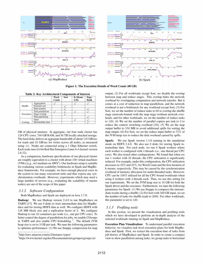
Table 7: Overall Results: K-MeansPlatform Spark MR Spark MR Spark MRInput size (million records) 1 1 200 200 1000 1000Iteration time 1st 13s 20s 1.6m 2.3m 8.4m 9.4mIteration time Subseq. 3s 20s 26s 2.3m 2.1m 10.6mMedian map task time 1st 11s 19s 15s 46s 15s 46sMedian reduce task time 1st 1s 1s 1s 1s 8s 1sMedian map task time Subseq. 2s 19s 4s 46s 4s 50sMedian reduce task time Subseq. 1s 1s 1s 1s 3s 1sCached input data (GB) 0.2 - 41.0 - 204.9 -
optimization covers a large set of iterative machine learning algo-rithms such as linear regression, logistic regression, and supportvector machine. Therefore, the observations we draw from the re-sults presented in this section for k-means are generally applicableto the above mentioned algorithms.
As shown in Table 1, both the shuffle selectivity and the iterationselectivity of k-means is low. Suppose there are N input recordsto train K centroids, both map output (for each task) and job out-put only have K records . Since K is often much smaller than N ,both the shuffle and iteration selectivities are very small. As shownin Table 2, the training data can be cached in-memory for subse-quent iterations. This is common in machine learning algorithms.Therefore, we use k-means to evaluate the caching component.
3.4.1 Overall ResultTable 7 presents the overall results for k-means for various in-
put sizes, for both Spark and MapReduce. For the first iteration,Spark is about 1.5x faster than MapReduce. For subsequent itera-tions, because of RDD caching, Spark is more than 5x faster thanMapReduce for all input sizes.
We compare the performance of various RDD caching options(i.e., storage levels) available in Spark, and we find that the effec-tiveness of all the persistence mechanisms is almost the same forthis workload. We explain the reason in Section 3.4.3.
Another interesting observation is that when there is no in-heapcaching (i.e., for Spark without RDD caching and MapReduce), thedisk I/O decreases from one iteration to the next iteration becauseof the increased hit ratio of OS buffer cache for input from HDFS.However, this does not result in a reduction in the execution time.We explain these observations in Section 3.4.4.
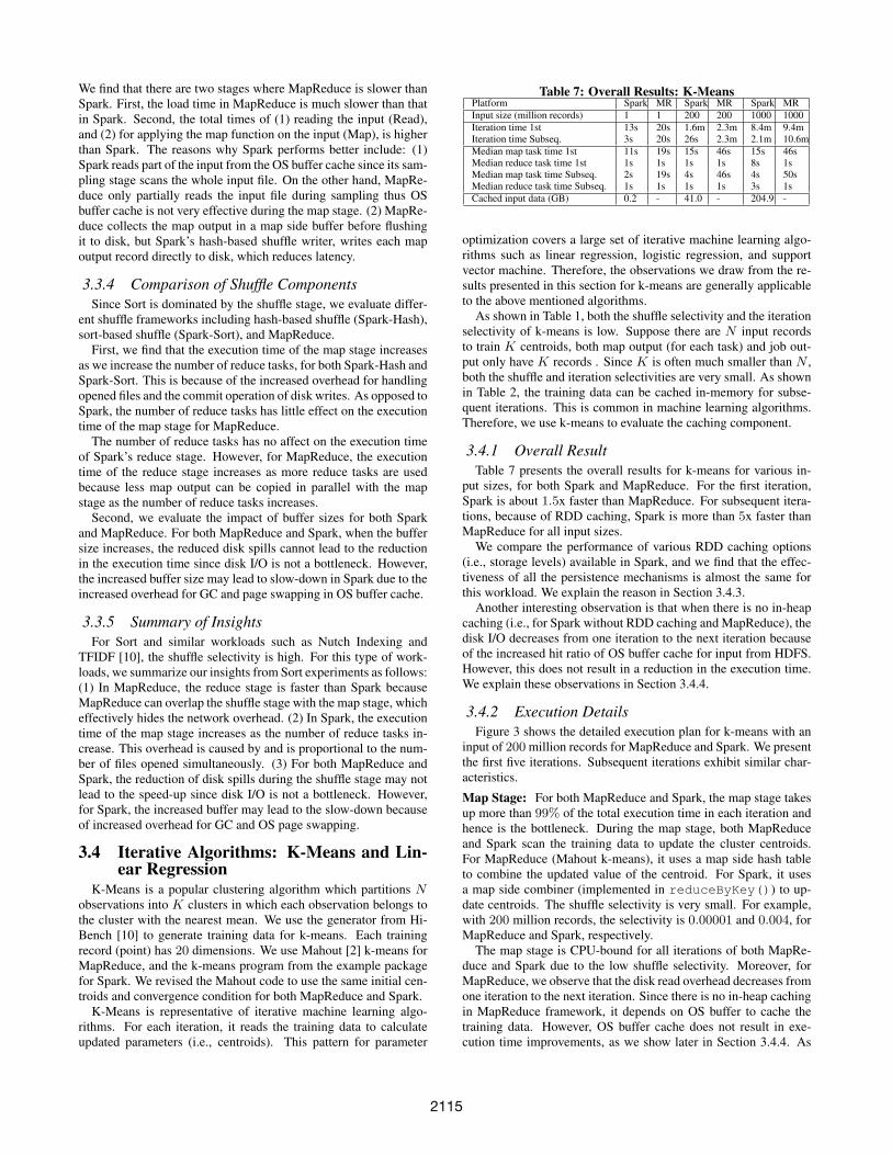
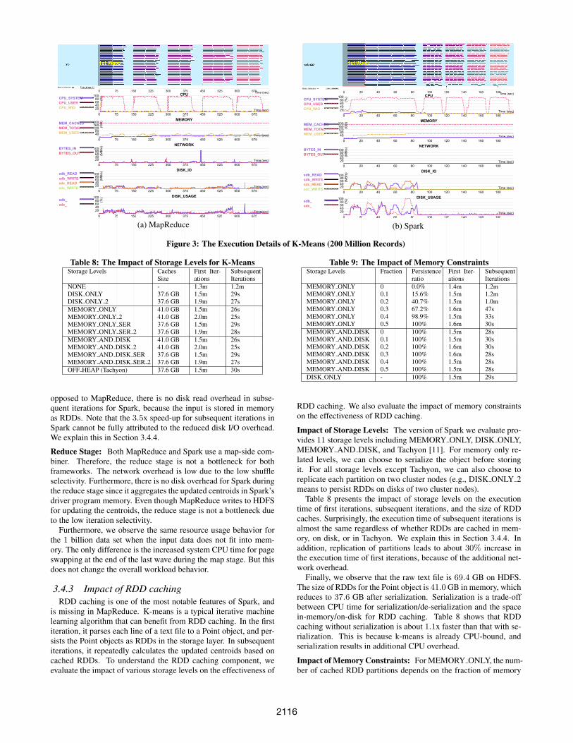
3.4.2 Execution DetailsFigure 3 shows the detailed execution plan for k-means with an
input of 200 million records for MapReduce and Spark. We presentthe first five iterations. Subsequent iterations exhibit similar char-acteristics.
Map Stage: For both MapReduce and Spark, the map stage takesup more than 99% of the total execution time in each iteration andhence is the bottleneck. During the map stage, both MapReduceand Spark scan the training data to update the cluster centroids.For MapReduce (Mahout k-means), it uses a map side hash tableto combine the updated value of the centroid. For Spark, it usesa map side combiner (implemented in reduceByKey()) to up-date centroids. The shuffle selectivity is very small. For example,with 200 million records, the selectivity is 0.00001 and 0.004, forMapReduce and Spark, respectively.
The map stage is CPU-bound for all iterations of both MapRe-duce and Spark due to the low shuffle selectivity. Moreover, forMapReduce, we observe that the disk read overhead decreases fromone iteration to the next iteration. Since there is no in-heap cachingin MapReduce framework, it depends on OS buffer to cache thetraining data. However, OS buffer cache does not result in exe-cution time improvements, as we show later in Section 3.4.4. As
2115
Metric Selection
CPU_SYSTEM
CPU_USER
CPU_WIO
MEM_CACHED
MEM_TOTAL
MEM_USED
BYTES_IN
BYTES_OUT
sdb_READ
sdb_WRITE
sdc_READ
sdc_WRITE
sdb_
sdc_
0 75 150 225 300 375 450 525 600 675Time (sec)
0 75 150 225 300 375 450 525 600 675
Time (sec)20406080100
(%) CPU
0%
0 75 150 225 300 375 450 525 600 675
Time (sec)4080120160200
(GB) MEMORY
0 75 150 225 300 375 450 525 600 675
Time (sec)20406080100
(MB/s) NETWORK
0 75 150 225 300 375 450 525 600 675
Time (sec)20406080100
(MB/s) DISK_IO
0 75 150 225 300 375 450 525 600 675
Time (sec)20406080100
(%) DISK_USAGE
(a) MapReduce
Metric Selection
CPU_SYSTEM
CPU_USER
CPU_WIO
MEM_CACHED
MEM_TOTAL
MEM_USED
BYTES_IN
BYTES_OUT
sdb_READ
sdb_WRITE
sdc_READ
sdc_WRITE
sdb_
sdc_
0 20 40 60 80 100 120 140 160 180Time (sec)
0 20 40 60 80 100 120 140 160 180
Time (sec)20406080100
(%) CPU
0 20 40 60 80 100 120 140 160 180
Time (sec)4080120160200
(GB) MEMORY
0 20 40 60 80 100 120 140 160 180
Time (sec)20406080100
(MB/s) NETWORK
0 20 40 60 80 100 120 140 160 180
Time (sec)20406080100
(MB/s) DISK_IO
0 20 40 60 80 100 120 140 160 180
Time (sec)20406080100
(%) DISK_USAGE
(b) Spark
Figure 3: The Execution Details of K-Means (200 Million Records)
Table 8: The Impact of Storage Levels for K-MeansStorage Levels Caches
SizeFirst Iter-ations
SubsequentIterations
NONE - 1.3m 1.2mDISK ONLY 37.6 GB 1.5m 29sDISK ONLY 2 37.6 GB 1.9m 27sMEMORY ONLY 41.0 GB 1.5m 26sMEMORY ONLY 2 41.0 GB 2.0m 25sMEMORY ONLY SER 37.6 GB 1.5m 29sMEMORY ONLY SER 2 37.6 GB 1.9m 28sMEMORY AND DISK 41.0 GB 1.5m 26sMEMORY AND DISK 2 41.0 GB 2.0m 25sMEMORY AND DISK SER 37.6 GB 1.5m 29sMEMORY AND DISK SER 2 37.6 GB 1.9m 27sOFF HEAP (Tachyon) 37.6 GB 1.5m 30s
opposed to MapReduce, there is no disk read overhead in subse-quent iterations for Spark, because the input is stored in memoryas RDDs. Note that the 3.5x speed-up for subsequent iterations inSpark cannot be fully attributed to the reduced disk I/O overhead.We explain this in Section 3.4.4.
Reduce Stage: Both MapReduce and Spark use a map-side com-biner. Therefore, the reduce stage is not a bottleneck for bothframeworks. The network overhead is low due to the low shuffleselectivity. Furthermore, there is no disk overhead for Spark duringthe reduce stage since it aggregates the updated centroids in Spark’sdriver program memory. Even though MapReduce writes to HDFSfor updating the centroids, the reduce stage is not a bottleneck dueto the low iteration selectivity.
Furthermore, we observe the same resource usage behavior forthe 1 billion data set when the input data does not fit into mem-ory. The only difference is the increased system CPU time for pageswapping at the end of the last wave during the map stage. But thisdoes not change the overall workload behavior.
3.4.3 Impact of RDD cachingRDD caching is one of the most notable features of Spark, and
is missing in MapReduce. K-means is a typical iterative machinelearning algorithm that can benefit from RDD caching. In the firstiteration, it parses each line of a text file to a Point object, and per-sists the Point objects as RDDs in the storage layer. In subsequentiterations, it repeatedly calculates the updated centroids based oncached RDDs. To understand the RDD caching component, weevaluate the impact of various storage levels on the effectiveness of
Table 9: The Impact of Memory ConstraintsStorage Levels Fraction Persistence
ratioFirst Iter-ations
SubsequentIterations
MEMORY ONLY 0 0.0% 1.4m 1.2mMEMORY ONLY 0.1 15.6% 1.5m 1.2mMEMORY ONLY 0.2 40.7% 1.5m 1.0mMEMORY ONLY 0.3 67.2% 1.6m 47sMEMORY ONLY 0.4 98.9% 1.5m 33sMEMORY ONLY 0.5 100% 1.6m 30sMEMORY AND DISK 0 100% 1.5m 28sMEMORY AND DISK 0.1 100% 1.5m 30sMEMORY AND DISK 0.2 100% 1.6m 30sMEMORY AND DISK 0.3 100% 1.6m 28sMEMORY AND DISK 0.4 100% 1.5m 28sMEMORY AND DISK 0.5 100% 1.5m 28sDISK ONLY - 100% 1.5m 29s
RDD caching. We also evaluate the impact of memory constraintson the effectiveness of RDD caching.
Impact of Storage Levels: The version of Spark we evaluate pro-vides 11 storage levels including MEMORY ONLY, DISK ONLY,MEMORY AND DISK, and Tachyon [11]. For memory only re-lated levels, we can choose to serialize the object before storingit. For all storage levels except Tachyon, we can also choose toreplicate each partition on two cluster nodes (e.g., DISK ONLY 2means to persist RDDs on disks of two cluster nodes).
Table 8 presents the impact of storage levels on the executiontime of first iterations, subsequent iterations, and the size of RDDcaches. Surprisingly, the execution time of subsequent iterations isalmost the same regardless of whether RDDs are cached in mem-ory, on disk, or in Tachyon. We explain this in Section 3.4.4. Inaddition, replication of partitions leads to about 30% increase inthe execution time of first iterations, because of the additional net-work overhead.
Finally, we observe that the raw text file is 69.4 GB on HDFS.The size of RDDs for the Point object is 41.0 GB in memory, whichreduces to 37.6 GB after serialization. Serialization is a trade-offbetween CPU time for serialization/de-serialization and the spacein-memory/on-disk for RDD caching. Table 8 shows that RDDcaching without serialization is about 1.1x faster than that with se-rialization. This is because k-means is already CPU-bound, andserialization results in additional CPU overhead.
Impact of Memory Constraints: For MEMORY ONLY, the num-ber of cached RDD partitions depends on the fraction of memory
2116
allocated to the MemoryStore, which is configurable. For otherstorage levels, when the size of MemoryStore exceeds the config-ured limit, RDDs which have to be persisted will be stored on disk.Table 9 presents the impact of memory constraints on the persis-tence ratio (i.e., the number of cached partitions / the number of allpartitions), execution time of first iterations, and execution time ofsubsequent iterations. The persistence ratio of MEMORY ONLYdecreases as less memory is allocated for MemoryStore. More-over, the persistence ratio rather than the storage level is the mainfactor that affects the execution time of subsequent iterations. Thisis consistent with the results shown in Table 8. From these re-sults, we conclude that there is no significant performance differ-ence when using different storage levels for k-means.
3.4.4 What is the bottleneck for kmeans?From the experiments, we make several non-trivial observations
for k-means: (a) The storage levels do not impact the executiontime of subsequent iterations. (b) For DISK ONLY, there are al-most no disk reads in subsequent iterations. (c) When there is noRDD caching, disk reads decrease from one iteration to the nextiteration, but this does not lead to execution time improvements.
To explain these observations and further understand RDDcaching in Spark, we conduct the following micro-benchmark ex-periments. We use DISK ONLY as the baseline. (1) We set thefraction of Java heap for MemoryStore to 0 MB. Compared to thebaseline, there is no difference in execution time and memory con-sumption. This means that DISK ONLY does not store any RDDsin Java heap. (2) We reduce the number of disks for storing inter-mediate data (i.e., RDD caching) from 8 to 1. The execution timeis still the same as the baseline, but we observe that the disk uti-lization increases by about 8x on the retained disk compared to thebaseline. This means that disks are far from 100% utilized whenwe have 8 disks to store intermediate data. (3) We reduce memoryof executors from 32 GB to 200 MB. The execution time is 17%slower compared to the baseline. This is because of the increasedGC overhead. Note that there is still no disk read in subsequentiterations. (4) We drop OS buffer cache after the first iteration. Weobserve that the execution time of the subsequent iteration is in-creased from 29 seconds to 53 seconds. Moreover, we find heavydisk reads after OS buffer cache is dropped. The retained disk is100% utilized, and 80% of CPU time becomes iowait time. Thismeans that RDDs are cached in pages of the OS buffer after the firstiteration when we use DISK ONLY. (5) To further evaluate the per-formance of DISK ONLY RDD caching without OS buffer cache,we restore 8 disks to store intermediate results. We also drop OSbuffer cache after the first iteration. We observe that the executiontime of the subsequent iteration is reduced from 53 seconds to 29seconds. There are still disk reads after OS buffer cache is dropped,but user CPU time is restored to 100%. This means that when alldisks are restored for RDD caching, disk reads are no longer thebottleneck even without OS buffer cache. With 8 disks, the aggre-gate disk bandwidth is more than enough to sustain the IO rate fork-means, with or without OS buffer cache.
However, these results lead to the following additional observa-tions: (d) When there is no RDD caching, OS buffer cache does notimprove the execution time. (e) In the case without RDD caching,disk reads decrease faster than with DISK ONLY RDD caching. Toexplain (c), (d), and (e), we design another set of micro-benchmarkexperiments to detect the bottleneck for iterations which read inputfrom HDFS. We first design a micro-benchmark to minimize theCPU overhead to evaluate the behavior of HadoopRDD (An RDDthat provides core functionality for reading data stored in Hadoop).The HadoopRDD is scanned and persisted in the first iteration, then
the cached RDDs are scanned with count() in subsequent itera-tions. For NONE (i.e., without RDD caching), we observe that theexecution time decreases in subsequent iterations as more blocksfrom HDFS are cached in the OS buffer. As opposed to k-means,the OS buffer cache reduces the execution time of subsequent iter-ations, since disk reads is the bottleneck for this micro-benchmark.Further, because of data locality, the hit ratio of OS buffer cache isabout 100% in the second iteration for DISK ONLY, but that ratiois about only 30% for NONE. When HDFS caching [3] is enabled,the execution time of subsequent iterations decreases as more repli-cas are stored in the HDFS cache. From the above experiments, weestablished that the OS buffer cache improves the execution time ofsubsequent iterations if disk I/O is a bottleneck.
Next, we change a single line in k-means code to persistHadoopRDD before parsing lines to Point objects. We observe thatthe execution time of subsequent iterations is increased from 27and 29 seconds to 1.4 and 1.3 minutes, for MEMORY ONLY andDISK ONLY, respectively. Moreover, the disk utilization of sub-sequent iterations is the same as k-means and HadoopRDD scan.This indicates that the CPU overhead of parsing each line to thePoint object is the bottleneck for the first iteration that reads in-put from HDFS. Therefore, for k-means without RDD caching, thereduction of disk I/O due to OS buffer cache does not result in exe-cution time improvements for subsequent iterations, since the CPUoverhead of transforming the text to Point object is a bottleneck.
3.4.5 Linear RegressionWe also evaluated linear regression with maximum 1000000 ∗
50000 training records (372 GB), for both MapReduce and Spark.We observed the same behavior as k-means. Thus, we do not repeatthose details here. The only difference is that linear regression re-quires larger executor memory as compared to k-means. Therefore,the total size of the OS buffer cache and the JVM heap exceeds thememory limit on each node. This leads to about 30% system CPUoverhead for OS buffer cache swapping. This CPU overhead canbe eliminated by using DISK ONLY RDD caching which reducesmemory consumption.
3.4.6 Summary of InsightsA large set of iterative machine learning algorithms such as k-
means, linear regression, and logistic regression read the trainingdata to calculate a small set of parameters iteratively. For this typeof workloads, we summarize our insights from k-means as follows:(1) For iterative algorithms, if an iteration is CPU-bound, cachingthe raw file (to reduce disk I/O) may not help reduce the executiontime since the disk I/O is hidden by the CPU overhead. But on thecontrary, if an iteration is disk-bound, caching the raw file can sig-nificantly reduce the execution time. (2) RDD caching can reducenot only disk I/O, but also the CPU overhead since it can cacheany intermediate data during the analytic pipeline. For example,the main contribution of RDD caching for k-means is to cache thePoint object to save the transformation cost from a text line, whichis the bottleneck for each iteration. (3) If OS buffer is sufficient, thehit ratio of both OS buffer cache and HDFS caching for the trainingdata set increases from one iteration to the next iteration, becauseof the replica locality from previous iterations.
3.5 PageRankPageRank is a graph algorithm which ranks elements by count-
ing the number and quality of links. To evaluate PageRank algo-rithm on MapReduce and Spark, we use Facebook 5 and Twitter 6
5http://current.cs.ucsb.edu/facebook/index.html6http://an.kaist.ac.kr/traces/WWW2010.html
2117
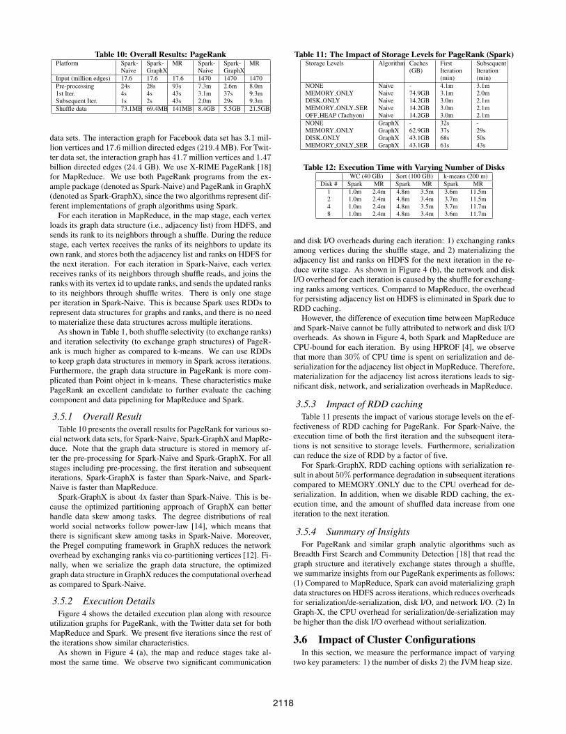
Table 10: Overall Results: PageRankPlatform Spark-
NaiveSpark-GraphX
MR Spark-Naive
Spark-GraphX
MR
Input (million edges) 17.6 17.6 17.6 1470 1470 1470Pre-processing 24s 28s 93s 7.3m 2.6m 8.0m1st Iter. 4s 4s 43s 3.1m 37s 9.3mSubsequent Iter. 1s 2s 43s 2.0m 29s 9.3mShuffle data 73.1MB 69.4MB 141MB 8.4GB 5.5GB 21.5GB
data sets. The interaction graph for Facebook data set has 3.1 mil-lion vertices and 17.6 million directed edges (219.4 MB). For Twit-ter data set, the interaction graph has 41.7 million vertices and 1.47billion directed edges (24.4 GB). We use X-RIME PageRank [18]for MapReduce. We use both PageRank programs from the ex-ample package (denoted as Spark-Naive) and PageRank in GraphX(denoted as Spark-GraphX), since the two algorithms represent dif-ferent implementations of graph algorithms using Spark.
For each iteration in MapReduce, in the map stage, each vertexloads its graph data structure (i.e., adjacency list) from HDFS, andsends its rank to its neighbors through a shuffle. During the reducestage, each vertex receives the ranks of its neighbors to update itsown rank, and stores both the adjacency list and ranks on HDFS forthe next iteration. For each iteration in Spark-Naive, each vertexreceives ranks of its neighbors through shuffle reads, and joins theranks with its vertex id to update ranks, and sends the updated ranksto its neighbors through shuffle writes. There is only one stageper iteration in Spark-Naive. This is because Spark uses RDDs torepresent data structures for graphs and ranks, and there is no needto materialize these data structures across multiple iterations.
As shown in Table 1, both shuffle selectivity (to exchange ranks)and iteration selectivity (to exchange graph structures) of PageR-ank is much higher as compared to k-means. We can use RDDsto keep graph data structures in memory in Spark across iterations.Furthermore, the graph data structure in PageRank is more com-plicated than Point object in k-means. These characteristics makePageRank an excellent candidate to further evaluate the cachingcomponent and data pipelining for MapReduce and Spark.
3.5.1 Overall ResultTable 10 presents the overall results for PageRank for various so-
cial network data sets, for Spark-Naive, Spark-GraphX and MapRe-duce. Note that the graph data structure is stored in memory af-ter the pre-processing for Spark-Naive and Spark-GraphX. For allstages including pre-processing, the first iteration and subsequentiterations, Spark-GraphX is faster than Spark-Naive, and Spark-Naive is faster than MapReduce.
Spark-GraphX is about 4x faster than Spark-Naive. This is be-cause the optimized partitioning approach of GraphX can betterhandle data skew among tasks. The degree distributions of realworld social networks follow power-law [14], which means thatthere is significant skew among tasks in Spark-Naive. Moreover,the Pregel computing framework in GraphX reduces the networkoverhead by exchanging ranks via co-partitioning vertices [12]. Fi-nally, when we serialize the graph data structure, the optimizedgraph data structure in GraphX reduces the computational overheadas compared to Spark-Naive.
3.5.2 Execution DetailsFigure 4 shows the detailed execution plan along with resource
utilization graphs for PageRank, with the Twitter data set for bothMapReduce and Spark. We present five iterations since the rest ofthe iterations show similar characteristics.
As shown in Figure 4 (a), the map and reduce stages take al-most the same time. We observe two significant communication
Table 11: The Impact of Storage Levels for PageRank (Spark)Storage Levels Algorithm Caches
(GB)FirstIteration(min)
SubsequentIteration(min)
NONE Naive - 4.1m 3.1mMEMORY ONLY Naive 74.9GB 3.1m 2.0mDISK ONLY Naive 14.2GB 3.0m 2.1mMEMORY ONLY SER Naive 14.2GB 3.0m 2.1mOFF HEAP (Tachyon) Naive 14.2GB 3.0m 2.1mNONE GraphX - 32s -MEMORY ONLY GraphX 62.9GB 37s 29sDISK ONLY GraphX 43.1GB 68s 50sMEMORY ONLY SER GraphX 43.1GB 61s 43s
Table 12: Execution Time with Varying Number of DisksWC (40 GB) Sort (100 GB) k-means (200 m)
Disk # Spark MR Spark MR Spark MR1 1.0m 2.4m 4.8m 3.5m 3.6m 11.5m2 1.0m 2.4m 4.8m 3.4m 3.7m 11.5m4 1.0m 2.4m 4.8m 3.5m 3.7m 11.7m8 1.0m 2.4m 4.8m 3.4m 3.6m 11.7m
and disk I/O overheads during each iteration: 1) exchanging ranksamong vertices during the shuffle stage, and 2) materializing theadjacency list and ranks on HDFS for the next iteration in the re-duce write stage. As shown in Figure 4 (b), the network and diskI/O overhead for each iteration is caused by the shuffle for exchang-ing ranks among vertices. Compared to MapReduce, the overheadfor persisting adjacency list on HDFS is eliminated in Spark due toRDD caching.
However, the difference of execution time between MapReduceand Spark-Naive cannot be fully attributed to network and disk I/Ooverheads. As shown in Figure 4, both Spark and MapReduce areCPU-bound for each iteration. By using HPROF [4], we observethat more than 30% of CPU time is spent on serialization and de-serialization for the adjacency list object in MapReduce. Therefore,materialization for the adjacency list across iterations leads to sig-nificant disk, network, and serialization overheads in MapReduce.
3.5.3 Impact of RDD cachingTable 11 presents the impact of various storage levels on the ef-
fectiveness of RDD caching for PageRank. For Spark-Naive, theexecution time of both the first iteration and the subsequent itera-tions is not sensitive to storage levels. Furthermore, serializationcan reduce the size of RDD by a factor of five.
For Spark-GraphX, RDD caching options with serialization re-sult in about 50% performance degradation in subsequent iterationscompared to MEMORY ONLY due to the CPU overhead for de-serialization. In addition, when we disable RDD caching, the ex-ecution time, and the amount of shuffled data increase from oneiteration to the next iteration.
3.5.4 Summary of InsightsFor PageRank and similar graph analytic algorithms such as
Breadth First Search and Community Detection [18] that read thegraph structure and iteratively exchange states through a shuffle,we summarize insights from our PageRank experiments as follows:(1) Compared to MapReduce, Spark can avoid materializing graphdata structures on HDFS across iterations, which reduces overheadsfor serialization/de-serialization, disk I/O, and network I/O. (2) InGraph-X, the CPU overhead for serialization/de-serialization maybe higher than the disk I/O overhead without serialization.
3.6 Impact of Cluster ConfigurationsIn this section, we measure the performance impact of varying
two key parameters: 1) the number of disks 2) the JVM heap size.
2118

Metric Selection
CPU_SYSTEM
CPU_USER
CPU_WIO
MEM_CACHED
MEM_TOTAL
MEM_USED
BYTES_IN
BYTES_OUT
sdb_READ
sdb_WRITE
sdc_READ
sdc_WRITE
sdb_
sdc_
0 330 660 990 1320 1650 1980 2310 2640 2970Time (sec)
0 330 660 990 1320 1650 1980 2310 2640 2970
Time (sec)20406080100
(%) CPU
0 330 660 990 1320 1650 1980 2310 2640 2970
Time (sec)4080120160200
(GB) MEMORY
0 330 660 990 1320 1650 1980 2310 2640 2970
Time (sec)20406080100
(MB/s) NETWORK
0 330 660 990 1320 1650 1980 2310 2640 2970
Time (sec)20406080100
(MB/s) DISK_IO
0 330 660 990 1320 1650 1980 2310 2640 2970
Time (sec)20406080100
(%) DISK_USAGE
(a) MapReduce
Metric Selection
CPU_SYSTEM
CPU_USER
CPU_WIO
MEM_CACHED
MEM_TOTAL
MEM_USED
BYTES_IN
BYTES_OUT
sdb_READ
sdb_WRITE
sdc_READ
sdc_WRITE
sdb_
sdc_
0 120 240 360 480 600 720 840 960 1080Time (sec)
0 120 240 360 480 600 720 840 960 1080
Time (sec)20406080100
(%) CPU
0 120 240 360 480 600 720 840 960 1080
Time (sec)4080120160200
(GB) MEMORY
0 120 240 360 480 600 720 840 960 1080
Time (sec)20406080100
(MB/s) NETWORK
0 120 240 360 480 600 720 840 960 1080
Time (sec)20406080100
(MB/s) DISK_IO
0 120 240 360 480 600 720 840 960 1080
Time (sec)20406080100
(%) DISK_USAGE
(b) Spark-Naive
Figure 4: The Execution Details of PageRank (Twitter Data)
3.6.1 Execution Time with Varying Number of DisksIn this set of experiments, we vary the number of disks used to
store intermediate data (i.e., map output for MapReduce and Spark,RDD caching on disk for Spark) to measure its impact on perfor-mance. We use DISK ONLY configuration for Spark k-means toensure that RDDs are cached on disk. As shown in Table 12, theexecution time for these workloads is not sensitive to the numberof disks for intermediate data storage. Also, through the analysis ofthe detailed execution plan, even for the single disk case, we findthat the disk is not fully utilized.
Next, we manually drop OS buffer cache during the executionof a job to ensure that the intermediate data is read from the disks.This has little impact on most of the workloads. The only excep-tion is Spark k-means when using only 1 disk for RDD caching.By breaking down the execution time for this case, we find thatclearing the OS cache results in approximately 80% performancedegradation for the next iteration.
From the above results, we conclude that disk I/O for intermedi-ate data is not a bottleneck for typical cluster configurations, for amajority of MapReduce and Spark workloads. On the other hand,for some extremely unbalanced cluster configurations (e.g., 24 CPUcores with 1 disk and no OS buffer cache), disk I/O becomes a bot-tleneck.
3.6.2 Impact of Memory LimitsIn the next set of experiments, we vary the JVM heap size to
evaluate the impact of various memory limits including the case inwhich data does not fit in main memory. For a fair comparison,we disable the overlap between map and reduce stages for MapRe-duce. We run these experiments with 40 GB WC, 100 GB Sortand 200 million records k-means. Table 13 presents the impact ofthe JVM heap size on the task execution time, the fraction of timespent in GC, and additional data spilling. All the metrics presentedin this table are median values among the tasks. We find that: (1)The fraction of GC time decreases as the JVM heap size increases,except for the reduce stage for Spark-Sort with 4 GB heap size pertask. This is caused by the additional overhead for OS page swap-ping (explained in Section 3.3.4); (2) When the JVM heap size islarger than 256 MB, the fraction of GC time becomes relatively sta-ble; (3) The execution time is not sensitive to additional data spillsto disks since disk I/O is not a bottleneck for WC and Sort, for both
Table 15: The Execution Times with Task FailuresSort (mapkilled)
Sort (reducekilled)
k-means (1st&4thiter killed)
Nf %killed
%slow-down
%killed
%slow-down
%killed
%slow-down(1st)
%slow-down(4th)
Spark
1 1.6% 2.1% 33.3% 108.3% 1.2% 7.1% 57.7%1 1.6% 6.3% 49.2% 129.2% 4.9% 14.3% 80.8%1 4% 6.3% 63.3% 129.2% 9.8% 14.3% 92.3%4 3.6% 4.2% 40% 81.3% 4.9% 7.1% 57.7%4 14.6% 6% 106% 62.5% 18.2% 21.4% 176.9%4 27.3% 12.5% 122% 70.8% 37.4% 42.9% 269.2%
MapReduce
1 0.5% 36.8% 3.3% 18.2% 1.3% 7.9% 7.1%1 1.9% 40.0% 13.3% 18.6% 5% 18.6% 6.4%1 3.1% 58.2% 25.8% 18.6% 10% 26.4% 27.9%4 1.9% 7.3% 13.3% 14.1% 5% 5.7% 2.9%4 7.3% 10.5% 26.75% 13.6% 20% 10.0% 6.4%4 10.5% 18.2% 53.3% 29.1% 39.7% 22.1% 24.3%
MapReduce and Spark. As shown in Table 14, the impact of theJVM heap size on k-means performance is very similar in compar-ison to WC and Sort. In summary, if tasks run with the JVM heapsize above a certain level (e.g., larger than 256 MB), the JVM heapsize will not significantly affect the execution time for most of theMapReduce and Spark workloads even with additional data spillsto disks.
3.7 FaultToleranceThis section evaluates the effectiveness of the built-in fault-
tolerance mechanisms in MapReduce and Spark. We present theresults for Sort and k-means in Table 15 (the results for other work-loads are similar). The killed tasks are evenly distributed on Nf
nodes, ranging from a single node to all four nodes in the clus-ter. These experiments confirm that both frameworks provide fault-tolerance for tasks. As shown in Table 15, when tasks are killedduring the reduce stage for Sort, the slow-down for Spark is muchworse than that for MapReduce. Comparing to MapReduce, whereonly reduce tasks are re-executed, in Spark the loss of an executorwill lead to the re-execution of the portion of map tasks which lostthe block information. Thus, a potential improvement for Spark isto increase the availability of the block information in case of fail-ure. In the experiments with k-means, tasks are killed during thefirst, and the fourth iteration. As shown in the rightmost column
2119
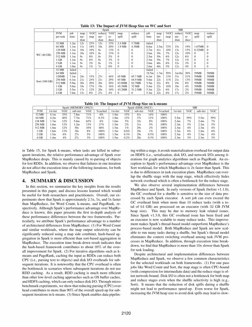
Table 13: The Impact of JVM Heap Size on WC and SortSpark MR
JVMper task
jobtime
mapme-dian
%GCmap
reduceme-dian
%GCre-duce
mapspill
reducespill
jobtime
mapme-dian
%GCmap
reduceme-dian
%GCre-duce
mapspill
reducespill
WC (40 GB)
32 MB 1.2m 12s 25% 12s 33% 2.4 MB 5.7MB failed - - - - - -64 MB 1.1m 11s 18% 10s 20% 1.9 MB 4.3MB 8.6m 2.5m 72% 15s 19% 1.67MB 0128 MB 1.1m 10s 10% 8s 13% 0 0 2.7m 41s 10% 13s 15% 0.32MB 0256 MB 1.1m 10s 10% 8s 13% 0 0 2.6m 39s 7% 12s 10% 0 0512 MB 1.1m 9s 8% 8s 5% 0 0 2.5m 39s 6% 12s 6% 0 01 GB 1.1m 9s 6% 8s 3% 0 0 2.5m 39s 7% 12s 1% 0 02 GB 1.1m 9s 2% 8s 1% 0 0 2.6m 40s 6% 12s 3% 0 04 GB 1.0m 9s 1% 7s 0% 0 0 2.6m 40s 5% 12s 4% 0 0
Sort (100 GB)
32 MB failed - - - - - - failed - - - - - -64 MB failed - - - - - - 19.5m 1.7m 59% 1m16s 30% 59MB 58MB128MB 7.1m 24s 33% 27s 44% 65 MB 65.7 MB 6.1m 20s 13% 31s 21% 59MB 58MB256 MB 6.1m 21s 24% 21s 29% 65 MB 64.9 MB 5.6m 22s 11% 21s 13% 59MB 58MB512 MB 5.9m 20s 20% 20s 20% 63.8MB 62.7MB 5.5m 22s 8% 19s 8% 59MB 58MB1 GB 5.6m 18s 17% 19s 16% 45.3MB 52 MB 5.4m 22s 10% 18s 4% 59MB 58MB2 GB 5.5m 17s 12% 20s 10% 43.2MB 51.2 MB 5.3m 22s 6% 17s 2% 59MB 58MB4 GB 7.6m 13s 8% 27s 4% 0 0 5.3m 22s 6% 17s 2% 59MB 58MB
Table 14: The Impact of JVM Heap Size on k-meansSpark (MEMORY ONLY) Spark (DISK ONLY) MR
JVM 1st-iter %GC sub-iter %GC %cached 1st-iter %GC sub-iter %GC %cached 1st-iter %GC sub-iter %GC32 MB 4.1m 35% 7.8m 71% 0% 1.9m 15% 41s 14% 100% - - - -64 MB 4.2m 40% 7.7m 71% 0.3% 1.8m 12% 37s 12% 100% 5.5m 59% 5.5m 59%
128 MB 1.7m 12% 5.6m 65% 6% 1.6m 5% 32s 8% 100% 2.4m 7% 2.4m 7%256 MB 1.6m 12% 1.2m 13% 27% 1.5m 2% 31s 5% 100% 2.3m 5% 2.3m 5%512 MB 1.6m 12% 50s 10% 68% 1.5m 1% 29s 2% 100% 2.3m 4% 2.3m 4%
1 GB 1.6m 13% 30s 8% 100% 1.5m 0.6% 29s 1% 100% 2.3m 6% 2.4m 6%2 GB 1.5m 6% 27s 5% 100% 1.5m 0.3% 29s 0.5% 100% 2.3m 4% 2.3m 4%4 GB 1.4m 4% 27s 3% 100% 1.5m 0.2% 28s 0.3% 100% 2.3m 3% 2.3m 3%
in Table 15, for Spark k-means, when tasks are killed in subse-quent iterations, the relative performance advantage of Spark overMapReduce drops. This is mainly caused by re-parsing of objectsfor lost RDDs. In addition, we observe that failures in one iterationdo not affect the execution time of the following iterations, for bothMapReduce and Spark.
4. SUMMARY & DISCUSSIONIn this section, we summarize the key insights from the results
presented in this paper, and discuss lessons learned which wouldbe useful for both researchers and practitioners. Overall, our ex-periments show that Spark is approximately 2.5x, 5x, and 5x fasterthan MapReduce, for Word Count, k-means, and PageRank, re-spectively. Although Spark’s performance advantage over MapRe-duce is known, this paper presents the first in-depth analysis ofthese performance differences between the two frameworks. Par-ticularly, we attribute Spark’s performance advantage to a numberof architectural differences from MapReduce: (1) For Word Countand similar workloads, where the map output selectivity can besignificantly reduced using a map side combiner, hash-based ag-gregation in Spark is more efficient than sort-based aggregation inMapReduce. The execution time break-down result indicates thatthe hash-based framework contributes to about 39% of the over-all improvement for Spark. (2) For iterative algorithms such as k-means and PageRank, caching the input as RDDs can reduce bothCPU (i.e., parsing text to objects) and disk I/O overheads for sub-sequent iterations. It is noteworthy that the CPU overhead is oftenthe bottleneck in scenarios where subsequent iterations do not useRDD caching. As a result, RDD caching is much more efficientthan other low-level caching approaches such as OS buffer caches,and HDFS caching, which can only reduce disk I/O. Through micro-benchmark experiments, we show that reducing parsing (CPU) over-head contributes to more than 90% of the overall speed-up for sub-sequent iterations in k-means. (3) Since Spark enables data pipelin-
ing within a stage, it avoids materialization overhead for output dataon HDFS (i.e., serialization, disk I/O, and network I/O) among it-erations for graph analytics algorithms such as PageRank. An ex-ception to Spark’s performance advantage over MapReduce is theSort workload, for which MapReduce is 2x faster than Spark. Thisis due to differences in task execution plans. MapReduce can over-lap the shuffle stage with the map stage, which effectively hidesnetwork overhead which is often a bottleneck for the reduce stage.
We also observe several implementation differences betweenMapReduce and Spark. In early versions of Spark (before v1.1.0),the GC overhead for a shuffle is sensitive to the size of data pro-cessed by each Spark executor. A sort job can even exceed theGC overhead limit when more than 10 reduce tasks (with a to-tal of 64 GB) are processed on an executor (with 32 GB JVMheap size). This may be due to memory leak related issues.Since Spark v1.3.0, this GC overhead issue has been fixed andan executor is now scalable to many reduce tasks. This improve-ment makes Spark’s thread-based model outperform MapReduce’sprocess-based model. Both MapReduce and Spark are now scal-able to run many tasks during a shuffle, but Spark’s thread modeleliminates the context switching overhead among task JVM pro-cesses in MapReduce. In addition, through execution time break-down, we find that MapReduce is more than 10x slower than Sparkfor task loading.
Despite architectural and implementation differences betweenMapReduce and Spark, we observe a few common characteristicsfor the selected workloads on both frameworks. (1) For one passjobs like Word Count and Sort, the map stage is often CPU-bound(with compression for intermediate data) and the reduce stage is of-ten network-bound. Disk I/O is often not a bottleneck for both mapand reduce stages even when the shuffle selectivity is high (e.g.,Sort). It means that the reduction of disk spills during a shufflemight not lead to performance speed-up. Even worse for Spark,increasing the JVM heap size to avoid disk spills may lead to slow-
2120
down because of unexpected overhead for GC and OS page swap-ping. (2) For typical machine learning (e.g., k-means and linearregression) and graph analytics (e.g., PageRank) algorithms, pars-ing text to objects is often the bottleneck for each iteration. RDDcaching addresses this issue effectively by reducing the CPU over-head for parsing. OS buffer cache and HDFS caching to eliminatedisk I/O, are ineffective from this perspective.
To establish the generality of our key insights, we evaluate WordCount, Sort, and k-means under varying cluster configurations in-cluding varying the number of disks (for storing intermediate data)and the JVM heap size. The results indicate that our findings,in particular, the identified system behavior is not sensitive tothese configurations in most cases: (1) for Spark, k-means usingDISK ONLY RDD caching remains CPU-bound when the numberof disks for storing RDD caches is reduced from 8 to 1 on eachnode; (2) for both MapReduce and Spark, the map stage of Sortis CPU-bound when there is only one disk used to store the mapoutput on each node; (3) for both MapReduce and Spark, there isno significant performance degradation for all the selected work-loads when the JVM heap size per task (using 128 MB input split)is reduced from 4 GB to 128 MB. In addition to these findings,we also identified a few cases where the bottleneck changes withvarying configuration: (1) GC overhead becomes a major bottle-neck when the JVM heap size per task is reduced to be less than 64MB, for both MapReduce and Spark; (2) disk I/O becomes the bot-tleneck when we perform disk-based RDD caching on nodes withextremely unbalanced I/O and CPU capacities.
We evaluated the effectiveness of fault-tolerance mechanismsbuilt in both MapReduce and Spark, during different stages for eachworkloads. A potential improvement for Spark is on the availabilityof the block information in case of an executor failure to avoid re-computation of the portion of tasks that lose the block informationin case of failure.
To the best of our knowledge, this is the first experimental studythat drills-down sufficiently to explain the reasons for performancedifferences, attributes these differences to architectural and imple-mentation differences, and summarizes the workload behaviors ac-cordingly. To summarize, our detailed analysis of the behavior ofthe selected workloads on the two frameworks would be of par-ticular interest to developers of core engines, system administra-tors/users, and researchers of MapReduce/Spark.Developers: The core-engine developer of MapReduce/Spark canimprove both the architecture and implementation through our ob-servations. To improve the architecture, Spark might: (1) supportthe overlap between two stages with the shuffle dependency to hidethe network overhead; (2) improve the availability of block infor-mation in case of an executor failure to avoid re-computation ofsome tasks from the previous stage. To catch up with the perfor-mance of Spark, the potential improvements to MapReduce are: (1)significantly reduce the task load time; (2) consider thread-basedparallelism among tasks to reduce the context switching overhead;(3) provide hash-based framework as an alternative to the sort-based shuffle; (4) consider caching the serialized intermediate datain memory, or on disk for reuse across multiple jobs.System Administrators/Users: The system administrators/userscould have an in-depth understanding about the system behaviorfor typical workloads under various configurations, and gain in-sights for system tuning from OS, JVM to MapReduce/Spark pa-rameters: (1) Once tuned properly, the majority of workloads areCPU-bound for both MapReduce and Spark, and hence are scal-able to the number of CPU cores. (2) For MapReduce, the networkoverhead during a shuffle can be hidden by overlapping the map andreduce stages. For Spark, the intermediate data should always be
compressed, because its shuffle cannot be overlapped. (3) For bothMapReduce and Spark, more attention should be paid to GC andOS page swapping overhead rather than additional disk spills. (4)For iterative algorithms in Spark, counter-intuitively, DISK ONLYconfiguration might be better than MEMORY ONLY. Because bothof them address the object parsing bottleneck, but the former avoidsGC and page swapping issues by eliminating memory consumptionwhich makes it scalable to very large data sets.Researchers: The detailed analysis of workload behaviors char-acterize the nature of physical execution plans for both MapReduceand Spark. The researchers can further derive the trade-offs duringthe execution of a MapReduce or Spark jobs such as (1) trade-offbetween parallelism and context switching, (2) trade-off betweenin-memory and on-disk caching, and (3) trade-off between serial-ization and memory consumption. These trade-offs are the founda-tions for researchers to explore new cost models [9, 16] for MapRe-duce and Spark, which could be widely used for optimizations suchas self-tuning jobs and capacity planning on the cloud.
5. REFERENCES[1] Apache Hadoop. http://hadoop.apache.org/.[2] Apache Mahout. https://mahout.apache.org/.[3] HDFS caching. http://hadoop.apache.org/docs/current/hadoop-
project-dist/hadoop-hdfs/CentralizedCacheManagement.html.[4] HPROF: A heap/cpu profiling tool.
http://docs.oracle.com/javase/7/docs/technotes/samples/hprof.html.[5] RRDtool. http://oss.oetiker.ch/rrdtool/.[6] Spark wins 2014 graysort competition.
http://databricks.com/blog/2014/11/05/spark-officially-sets-a-new-record-in-large-scale-sorting.html.
[7] J. Dean and S. Ghemawat. Mapreduce: simplified data processing onlarge clusters. CACM, 51(1):107–113, 2008.
[8] P. Henderson. Functional Programming: Application andImplementation. Prentice-Hall International London, 1980.
[9] H. Herodotou and S. Babu. Profiling, what-if analysis, andcost-based optimization of mapreduce programs. VLDB,4(11):1111–1122, 2011.
[10] S. Huang, J. Huang, J. Dai, T. Xie, and B. Huang. The hibenchbenchmark suite: Characterization of the mapreduce-based dataanalysis. In ICDEW, pages 41–51, 2010.
[11] H. Li, A. Ghodsi, M. Zaharia, S. Shenker, and I. Stoica. Tachyon:Reliable, memory speed storage for cluster computing frameworks.In SOCC, pages 1–15, 2014.
[12] G. Malewicz, M. H. Austern, A. J. Bik, J. C. Dehnert, I. Horn,N. Leiser, and G. Czajkowski. Pregel: a system for large-scale graphprocessing. In SIGMOD, pages 135–146, 2010.
[13] M. L. Massie, B. N. Chun, and D. E. Culler. The ganglia distributedmonitoring system: design, implementation, and experience. ParallelComputing, 30(7):817–840, 2004.
[14] A. Mislove, M. Marcon, K. Gummadi, P. Druschel, andB. Bhattacharjee. Measurement and analysis of online socialnetworks. In IMC, pages 29–42, 2007.
[15] O. OMalley and A. C. Murthy. Winning a 60 second dash with ayellow elephant. Sort Benchmark, 2009.
[16] J. Shi, J. Zou, J. Lu, Z. Cao, S. Li, and C. Wang. MRTuner: A toolkitto enable holistic optimization for mapreduce jobs. VLDB,7(13):1319–1330, 2014.
[17] V. K. Vavilapalli, A. C. Murthy, C. Douglas, S. Agarwal, M. Konar,R. Evans, T. Graves, J. Lowe, H. Shah, S. Seth, B. Saha, C. Curino,O. O’Malley, S. Radia, B. Reed, and E. Baldeschwieler. ApacheHadoop YARN: Yet another resource negotiator. In SOCC, pages5:1–5:16, 2013.
[18] W. Xue, J. Shi, and B. Yang. X-RIME: Cloud-based large scale socialnetwork analysis. In SCC, pages 506–513, 2010.
[19] M. Zaharia, M. Chowdhury, T. Das, A. Dave, J. Ma, M. McCauley,M. J. Franklin, S. Shenker, and I. Stoica. Resilient distributeddatasets: A fault-tolerant abstraction for in-memory clustercomputing. In NSDI, 2012.
2121