Embed Size (px)
Citation preview
2009 Spring ME451 - GGZ Page 1Week 14-15: Frequency Design
Control Design based upon
• RL (Root Locus)
• Frequency Response Design– Bode Diagram (BD)
– Nyquist Approach
Control Design (CD) Control Design (CD) –– Control Design ProcessControl Design Process
1. Modeling
Mathematical modelMathematical model
2. Analysis
ControllerController
3. Design/Synthesis
4. Implementation
PlantPlantOutputOutput
ActuatorActuatorControllerController
SensorSensor
InputInput
Control Method to be discussed:
• PID control
• Gain compensation
• Phase lead/lag compensation
• Lead/lag compensation
2009 Spring ME451 - GGZ Page 2Week 14-15: Frequency Design
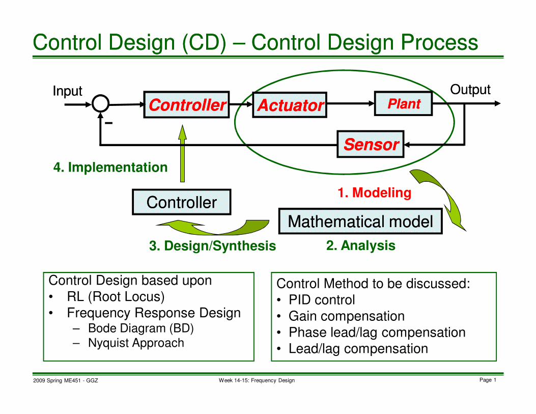
-
tt--domain:domain:
ss--domain:domain:
CD CD –– PID ControllerPID Controller
)(ty)(sP
)(tr
sKi/
pK
sKd
4342143421321
DerivativeIntegal
0alProportion
)()()()(
dt
tdeKdeKteKtu
d
t
ip++= ∫ ττ
++=++= sK
sKKsK
s
KKsC
D
I
pd
i
p
11)(
)(te)(tu

2009 Spring ME451 - GGZ Page 3Week 14-15: Frequency Design
• Most popular in process and robotics industries
– Good performance
– Functional simplicity (Operators can easily tune.)
• To avoid high frequency noise amplification, derivative term
is implemented as
with τd much smaller than plant time constant.
• PI controller
• PD controller
CD CD –– PID Controller RemarksPID Controller Remarks
1+≈
s
sKsK
d
d
dτ
s
KKsC i
p+=)(
sKKsCdp
+=)(

2009 Spring ME451 - GGZ Page 4Week 14-15: Frequency Design
• We plot y(t) for step reference r(t) with
– P controller
– PI controller
– PID controller
CD CD –– A Simple Example A Simple Example (1)(1)
-
)(ty)(sP
)(tr
sKi/
pK
sKd
)(te)(tu
3)1(
1)(
+=
ssP

2009 Spring ME451 - GGZ Page 5Week 14-15: Frequency Design
• Simple
• Steady state error
– Higher gain gives
smaller error
• Stability
– Higher gain gives
faster and more
oscillatory response
0 5 10 15 200
0.2
0.4
0.6
0.8
1
1.2
1.4
CD CD –– A Simple Example A Simple Example (P Controller (2))(P Controller (2))
pKsC =)(
1=p
K
2=p
K
5=p
K

2009 Spring ME451 - GGZ Page 6Week 14-15: Frequency Design
0 5 10 15 200
0.2
0.4
0.6
0.8
1
1.2
1.4
1.6
• Zero steady state error
(provided that CL is
stable.)
• Stability
– Higher gain gives
faster and more
oscillatory response
CD CD –– A Simple Example A Simple Example (PI Controller (3))(PI Controller (3))
s
KKsC i
p+=)(1=
pK
1=iK
5.0=iK
2.0=i
K
0=iK

2009 Spring ME451 - GGZ Page 7Week 14-15: Frequency Design
0 5 10 15 200
0.5
1
1.5
2
• Zero steady state error
(due to integral control)
• Stability
– Higher gain gives
more damped
response
• Too high gain worsen
performance.
CD CD –– A Simple Example A Simple Example (PID Controller (4))(PID Controller (4))
sKs
KKsC
d
i
p++=)(5.1,5.2 ==
ipKK
0
1
2
4
=
=
=
=
d
d
d
d
K
K
K
K

2009 Spring ME451 - GGZ Page 8Week 14-15: Frequency Design
• Model-based
– Root locus
– Frequency response approach
– Useful only when a model is available
– Necessary if a system has to work at the first trial
• Empirical (without model)
– Ziegler-Nichols tuning rule (1942)
– Simple
– Useful even if a system is too complex to model
– Useful only when trial-and-error tuning is allowed
CD CD –– How to Turn PID ParametersHow to Turn PID Parameters

2009 Spring ME451 - GGZ Page 9Week 14-15: Frequency Design
• Step response method (for only stable systems)
tt
OpenOpen--loop step responseloop step response
Steepest tangentSteepest tangent
PID parametersPID parameters
CD CD –– ZieglerZiegler--Nichols PID Tuning Rules Nichols PID Tuning Rules (1)(1)
)1
1()( sTsT
KsCd
I
p++=
)(ty
τ
α− ττα
τα
α
5.02/2.1
3/9.0
/1
Type
PID
PI
P
TTKDIP

2009 Spring ME451 - GGZ Page 10Week 14-15: Frequency Design
• Ultimate sensitivity method
ClosedClosed--loop step responseloop step response
with a gain controller with a gain controller
Increase gain and find Increase gain and find KKcc
generating oscillation generating oscillation
(marginally stable case).(marginally stable case).
PID parametersPID parameters
CD CD –– ZieglerZiegler--Nichols PID Tuning Rules Nichols PID Tuning Rules (2)(2)
)1
1()( sTsT
KsCd
I
p++=
CCC
CC
C
DIP
TTKPID
TKPI
KP
TTK
125.05.06.0
8.04.0
5.0
Type
)(ty
CT
t

2009 Spring ME451 - GGZ Page 11Week 14-15: Frequency Design
0 2 4 6 8 10 12 14 16 18 200
0.2
0.4
0.6
0.8
1
1.2
1.4
1.6
• Step response method • Ultimate sensitivity
0 2 4 6 8 10 12 14 16 18 200
0.2
0.4
0.6
0.8
1
1.2
1.4
1.6
PP
PIPI
PIDPID
PP
PIPI
PIDPID
CD CD –– A Simple Example A Simple Example (Revisited (5))(Revisited (5))

2009 Spring ME451 - GGZ Page 12Week 14-15: Frequency Design
0 2 4 6 8 100
0.2
0.4
0.6
0.8
1
0.790.79--0.280.28
CD CD –– OL Step Response for OL Step Response for “Step Response method”“Step Response method”

2009 Spring ME451 - GGZ Page 13Week 14-15: Frequency Design
0 5 100
0.5
1
0 5 100
0.5
1
0 5 100
1
2
0 5 100
0.5
1
1.5
CD CD –– CL Step Responses forCL Step Responses for “Ultimate Sensitivity method”“Ultimate Sensitivity method”
1=P
K
4=P
K
2=P
K
8=P
K 8=C
K
7.3=C
T

2009 Spring ME451 - GGZ Page 14Week 14-15: Frequency Design
• One example: Using OP amp
--
++--
++
Exercise: Derive this!Exercise: Derive this!
CD CD –– PID Controller Realization PID Controller Realization
++
+−
sCRsCR
C
C
R
R
21
12
2
1
1
2 1
)(tvi )(tv
o
1C 2
C
2R
1R
3R
4R

2009 Spring ME451 - GGZ Page 15Week 14-15: Frequency Design
• PID control
– Most popular controller in industry
– Model-free methods for design are available.
– Simple controller structure
– Simple controller tuning
– Widely applicable
• Ziegler-Nichols tuning rules provide a starting point for
fine tuning, rather than final settings of controller
parameters in a single shot.
CD CD –– PID Control Summary and Exercise PID Control Summary and Exercise

2009 Spring ME451 - GGZ Page 16Week 14-15: Frequency Design
• Z: # of CL poles in open RHP
• P: # of OL poles in open RHP (given)
• N: # of clockwise encirclement around -1
by Nyquist plot of OL transfer function L(s)
(counted by using Nyquist plot of L(s))
Remark: N = -1: a counter-clockwise encirclement
CD CD –– Nyquist Stability Criterion (Review)Nyquist Stability Criterion (Review)
0: stable is system CL =+=⇔ NPZ

2009 Spring ME451 - GGZ Page 17Week 14-15: Frequency Design
• IF P=0 (i.e., if L(s) has no pole in open RHP or stable)
This fact is very important since openThis fact is very important since open--loop systems loop systems
in many practical problems have no pole in open RHP!in many practical problems have no pole in open RHP!
CD CD –– Nyquist Stability Criterion: A Special CaseNyquist Stability Criterion: A Special Case
0stable is system CL =+=⇔ NPZ:
0stable is system CL =⇔ N

2009 Spring ME451 - GGZ Page 18Week 14-15: Frequency Design
ReRe
ImIm
ReRe
ImIm
CL stableCL stable CL unstableCL unstable
CD CD –– Examples with P = 0 (stable OL system) Examples with P = 0 (stable OL system)
)( ωjL )( ωjL

2009 Spring ME451 - GGZ Page 19Week 14-15: Frequency Design
• Nyquist stability criterion gives not only absolute but also
relative stability.
– Absolute stability: Is the closed-loop system stable or
not? (Answer is yes or no.)
– Relative stability: How “much” is the closed-loop
system stable? (Margin of safety)
• Relative stability is important because a math model is
never accurate.
• How to measure relative stability?
– Use a “distance” from the critical point -1.
– Gain margin (GM) & Phase margin (PM)
CD CD –– Nyquist Stability Remarks Nyquist Stability Remarks
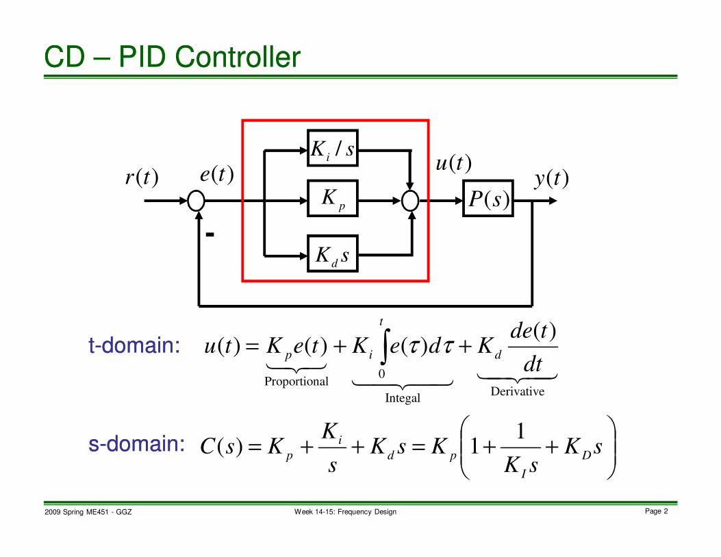
2009 Spring ME451 - GGZ Page 20Week 14-15: Frequency Design
• Phase crossover
frequency ωp:
• Gain margin (in dB)
• Indicates how much OL
gain can be multiplied
without violating CL
stability.
Nyquist plot of L(s)Nyquist plot of L(s)
CD CD –– Nyquist Gain Margin (GM) Nyquist Gain Margin (GM)
180)( −=∠p
jL ω
)(
1log20 10
pjLGM
ω=

2009 Spring ME451 - GGZ Page 21Week 14-15: Frequency Design
ReRe
ImIm
ReRe
ImIm
CD CD –– GM Examples GM Examples
dB6)(
1log20
2
10≈=
43421p
jLGM
ω
2
1)( −=
pjL ω
)( ωjL )( ωjL
3
1)( −=
pjL ω
dB5.9)(
1log20
3
10 ≈=
43421p
jLGM
ω

2009 Spring ME451 - GGZ Page 22Week 14-15: Frequency Design
Same gain margin,Same gain margin,
but different relative stabilitybut different relative stability
Gain margin is often inadequateGain margin is often inadequate
to indicate relative stabilityto indicate relative stability
Phase margin!Phase margin!
CD CD –– Why GM Alone is Inadequate Why GM Alone is Inadequate

2009 Spring ME451 - GGZ Page 23Week 14-15: Frequency Design
• Gain crossover
frequency ωg:
• Phase margin
• Indicates how much OL
phase can be added
without violating CL
stability.
Nyquist plot of L(s)Nyquist plot of L(s)
CD CD –– Nyquist Phase Margin (PM) Nyquist Phase Margin (PM)
1)( =∠g
jL ω
o
gjLPM 180)( +∠= ω

2009 Spring ME451 - GGZ Page 24Week 14-15: Frequency Design
CD CD –– PM Example PM Example
)50)(5(
2500)(
++=
ssssL
dB80.14182.0
1log20
10==GM

2009 Spring ME451 - GGZ Page 25Week 14-15: Frequency Design
• Advantages
– Nyquist plot can be used for study of closed-loop
stability, for open loop systems which is unstable and
includes time-delay.
• Disadvantage
– Controller design on Nyquist plot is difficult.
(Controller design on Bode plot is much simpler.)
We translate GM and PM on Nyquist plot We translate GM and PM on Nyquist plot
into those in Bode plot!into those in Bode plot!
CD CD –– Nyquist Plot Remarks Nyquist Plot Remarks

2009 Spring ME451 - GGZ Page 26Week 14-15: Frequency Design
ωωgg
ωωpp
GMGM
PMPM
CD CD –– Bode Diagram Relative Stability Bode Diagram Relative Stability
)( ωjL∠
)(log2010
ωjL
ω
ω

2009 Spring ME451 - GGZ Page 27Week 14-15: Frequency Design
• Advantages
– Without computer, Bode plot can be sketched easily.
– GM, PM, crossover frequencies are easily determined
on Bode plot.
– Controller design on Bode plot is simple.
• Disadvantage
– If OL system is unstable, we cannot use Bode plot for
stability analysis.
CD CD –– Bode Diagram Remarks Bode Diagram Remarks

2009 Spring ME451 - GGZ Page 28Week 14-15: Frequency Design
100
101
102
103
-100
-50
0
100
101
102
103
-180
-270
ωωgg ωωpp
GMGM
PMPM
CD CD –– Bode Diagram Example Bode Diagram Example
)50)(5(
2500)(
++=
ssssL

2009 Spring ME451 - GGZ Page 29Week 14-15: Frequency Design
10-1
100
-20
0
20
10-1
100
-180
-90
PMPM
GMGM
Time delay reducesTime delay reduces
relative stability!relative stability!
Delay timeDelay time
CD CD –– Bode Diagram Relative Stability Bode Diagram Relative Stability (time Delay)(time Delay)
)2)(1(
1)(
++=
ssssL
)2)(1()(
++=
−
sss
esL
s
lag phase deg 3.57 dTω

2009 Spring ME451 - GGZ Page 30Week 14-15: Frequency Design
1 0-2
1 0-1
1 00
1 01
1 02
-1
-0 .5
0
0 .5
1
1 0-2
1 0-1
1 00
1 01
1 02
-6 0 0 0
-4 0 0 0
-2 0 0 0
0
• TF
Huge phase lag!Huge phase lag!
As can be explained with Nyquist stability criterion, As can be explained with Nyquist stability criterion,
this phase lag causes instability of the closedthis phase lag causes instability of the closed--loop system,loop system,
and hence, the difficulty in control.and hence, the difficulty in control.
(rad) )( , ,1)()( TjGjGesGTs ωωωω −=∠∀=⇒= −
CD CD –– Body Diagram of A Time DelayBody Diagram of A Time Delay
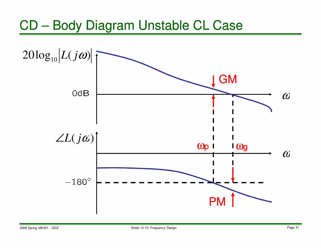
2009 Spring ME451 - GGZ Page 31Week 14-15: Frequency Design
ωωggωωpp
GMGM
PMPM
CD CD –– Body Diagram Unstable CL Case Body Diagram Unstable CL Case
ω
ω
)( ωjL∠
)(log2010
ωjL

2009 Spring ME451 - GGZ Page 32Week 14-15: Frequency Design
• Relative stability: Closeness of Nyquist plot to the critical
point -1
– Gain margin, phase crossover frequency
– Phase margin, gain crossover frequency
• Relative stability on Bode plot
• We normally emphasize PM in controller design.
CD CD –– Body Diagram Summary and Exercises Body Diagram Summary and Exercises

2009 Spring ME451 - GGZ Page 33Week 14-15: Frequency Design
Design specifications in time domainDesign specifications in time domain
(Rise time, settling time, overshoot, steady state error, etc.)(Rise time, settling time, overshoot, steady state error, etc.)
Desired closedDesired closed--loop loop
pole location pole location
in sin s--domaindomain
Constraints on openConstraints on open--loop loop
frequency response frequency response
in sin s--domaindomain
Root locus shapingRoot locus shaping Frequency response shapingFrequency response shaping
(Loop shaping)(Loop shaping)
Approximate translationApproximate translation
CD CD –– Control Design Comparison Control Design Comparison

2009 Spring ME451 - GGZ Page 34Week 14-15: Frequency Design
• Given G(s), design C(s) that satisfies time domain specs,
such as stability, transient, and steady-state responses.
• We learn typical qualitative relationships between open-
loop Bode plot and time-domain specifications.
PlantPlantControllerController
OL:OL:
CL:CL:
CD CD –– Feedback Control System Design Feedback Control System Design
)(ty)(tr)(sG)(sC
)()(:)( sCsGsL =
)(1
)(:)(
sL
sLsT
+=

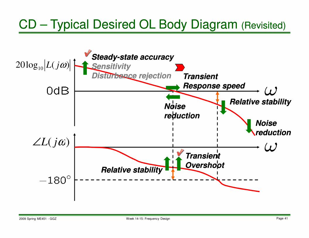
2009 Spring ME451 - GGZ Page 35Week 14-15: Frequency Design
SteadySteady--state accuracystate accuracy
SensitivitySensitivity
Disturbance rejectionDisturbance rejection
Noise Noise
reductionreduction
TransientTransient
Response speedResponse speed
Transient Transient
OvershootOvershootRelative stabilityRelative stability
Relative stabilityRelative stabilityNoise Noise
reductionreduction
CD CD –– Typical Desired OL Body DiagramTypical Desired OL Body Diagram
)( ωjL∠
)(log2010
ωjL

2009 Spring ME451 - GGZ Page 36Week 14-15: Frequency Design
For steadyFor steady--state accuracy, state accuracy,
L should have high gain at low frequencies.L should have high gain at low frequencies.
yy((tt)) tracks tracks rr((tt)) composed of composed of
low frequencies very well.low frequencies very well.
CD CD –– Steady State Accuracy Steady State Accuracy (1)(1)
PlantPlantControllerController
OL:OL:
CL:CL:
)(ty)(tr)(sG)(sC
)()(:)( sCsGsL =
)(1
)(:)(
sL
sLsT
+=
)( Large ωjL)(log2010
ωjL
1)(1
)()( ≈
+=
ω
ωω
jL
jLjY

2009 Spring ME451 - GGZ Page 37Week 14-15: Frequency Design
• Step r(t)
Increase
• Ramp r(t)
Increase • Parabolic r(t)
Increase
For Kv to be nonzero,For Kv to be nonzero,
L must contain L must contain
at least one integrator.at least one integrator.
For Ka to be nonzero,For Ka to be nonzero,
L must contain L must contain
at least two integrators.at least two integrators.
<<--2020 <<--4040
CD CD –– Steady State Accuracy (2)Steady State Accuracy (2)
)0(: LKp
=
)(log2010
ωjL )(log2010
ωjL )(log2010
ωjL
ω ω ω
)(lim:0
ssLKs
v→
= )(lim: 2
0sLsK
sa
→=

2009 Spring ME451 - GGZ Page 38Week 14-15: Frequency Design
Noise Noise
reductionreduction
TransientTransient
Response speedResponse speed
Transient Transient
OvershootOvershootRelative stabilityRelative stability
Relative stabilityRelative stabilityNoise Noise
reductionreduction
SteadySteady--state accuracystate accuracy
SensitivitySensitivity
Disturbance rejectionDisturbance rejection
CD CD –– Typical Desired OL Body Diagram Typical Desired OL Body Diagram (Revisited)(Revisited)
)( ωjL∠
)(log2010
ωjL

2009 Spring ME451 - GGZ Page 39Week 14-15: Frequency Design
• For illustration, we use the feedback system:
CD CD –– A 2A 2ndnd Order System ExampleOrder System Example
PlantPlantControllerController
)(ty)(tr)(sG)(sC
)2()()(:)(
2
n
n
sssCsGsL
ςω
ω
+==
22
2
2)(1
)(:)(
nn
n
sssL
sLsT
ωςω
ω
++=
+=

2009 Spring ME451 - GGZ Page 40Week 14-15: Frequency Design
0 5 10 150
0.2
0.4
0.6
0.8
1
1.2
1.4
1.6
1.8
For small percent overshoot, For small percent overshoot,
L should have larger phase margin.L should have larger phase margin.
10-1
100
101
-20
0
20
10-1
100
101
-180
-160
-140
-120
-100
CL step responseCL step responseOL Bode plotOL Bode plot
PMPM
CD CD –– Percent OvershootPercent Overshoot
1=n
ω5.0
3.0
1.0
=
=
=
ς
ς
ς
2009 Spring ME451 - GGZ Page 41Week 14-15: Frequency Design
Noise Noise
reductionreduction
TransientTransient
Response speedResponse speed
Transient Transient
OvershootOvershootRelative stabilityRelative stability
Relative stabilityRelative stabilityNoise Noise
reductionreduction
SteadySteady--state accuracystate accuracy
SensitivitySensitivity
Disturbance rejectionDisturbance rejection
CD CD –– Typical Desired OL Body Diagram Typical Desired OL Body Diagram (Revisited)(Revisited)
)( ωjL∠
)(log2010
ωjL

2009 Spring ME451 - GGZ Page 42Week 14-15: Frequency Design
0 5 10 150
0.2
0.4
0.6
0.8
1
1.2
1.4
100
-20
0
20
10-1
100
101
-180
-160
-140
-120
-100
For fast response, For fast response,
L should have larger gain crossover frequency.L should have larger gain crossover frequency.
CL step responseCL step responseOL Bode plotOL Bode plot
CD CD –– Response SpeedResponse Speed
3.0=ς3
2
1
=
=
=
n
n
n
ω
ω
ω

2009 Spring ME451 - GGZ Page 43Week 14-15: Frequency Design
Noise Noise
reductionreduction
TransientTransient
Response speedResponse speed
Transient Transient
OvershootOvershootRelative stabilityRelative stability
Relative stabilityRelative stabilityNoise Noise
reductionreduction
SteadySteady--state accuracystate accuracy
SensitivitySensitivity
Disturbance rejectionDisturbance rejection
CD CD –– Typical Desired OL Body Diagram Typical Desired OL Body Diagram (Revisited)(Revisited)
)( ωjL∠
)(log2010
ωjL
ω
ω
ω

2009 Spring ME451 - GGZ Page 44Week 14-15: Frequency Design
• We require adequate GM and PM for:
– safety against inaccuracies in modeling
– reasonable transient response
• It is difficult to give reasonable numbers of GM and PM for
general cases, but usually,
– GM should be at least 6dB
– PM should be at least 45deg
(These values are not absolute but approximate!)
• In controller design, we are especially interested in PM
(which typically gives good GM).
CD CD –– Relative StabilityRelative Stability
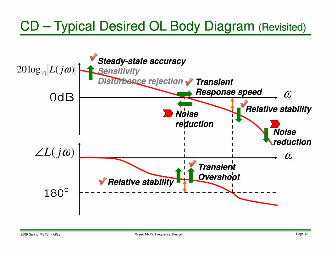
2009 Spring ME451 - GGZ Page 45Week 14-15: Frequency Design
Noise Noise
reductionreduction
TransientTransient
Response speedResponse speed
Transient Transient
OvershootOvershootRelative stabilityRelative stability
Relative stabilityRelative stabilityNoise Noise
reductionreduction
SteadySteady--state accuracystate accuracy
SensitivitySensitivity
Disturbance rejectionDisturbance rejection
CD CD –– Typical Desired OL Body Diagram Typical Desired OL Body Diagram (Revisited)(Revisited)
)( ωjL∠
)(log2010
ωjL
ω
ω
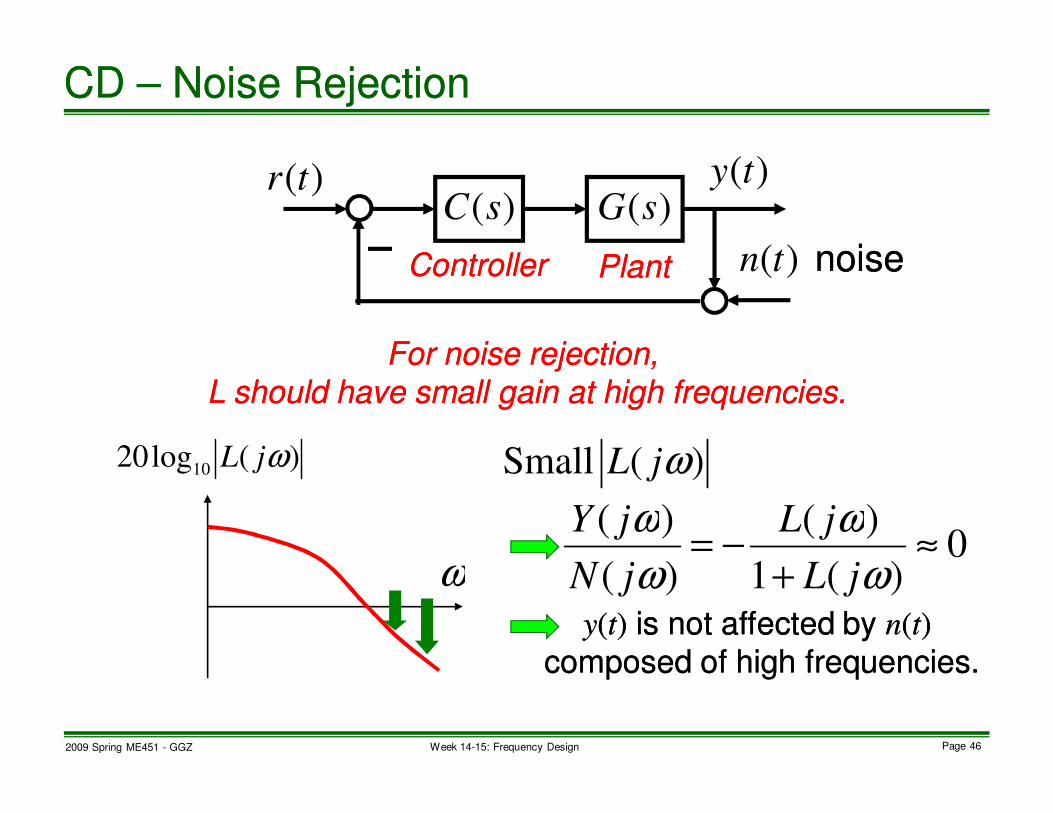
2009 Spring ME451 - GGZ Page 46Week 14-15: Frequency Design
yy((tt)) is not affected by is not affected by nn((tt))
composed of high frequencies.composed of high frequencies.
noisenoise
For noise rejection, For noise rejection,
L should have small gain at high frequencies.L should have small gain at high frequencies.
CD CD –– Noise RejectionNoise Rejection
PlantPlantControllerController
)(ty)(tr)(sG)(sC
)(tn
)( Small ωjL)(log2010
ωjL
0)(1
)(
)(
)(≈
+−=
ω
ω
ω
ω
jL
jL
jN
jY
ω
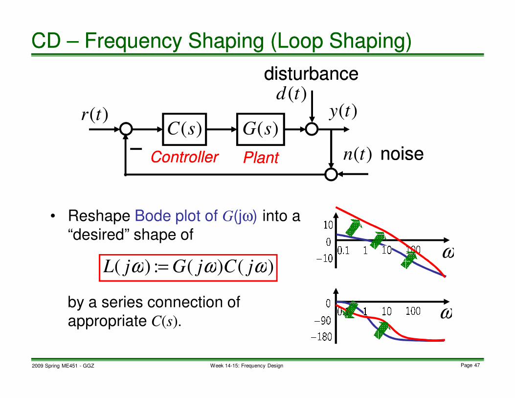
2009 Spring ME451 - GGZ Page 47Week 14-15: Frequency Design
• Reshape Bode plot of G(jω) into a
“desired” shape of
by a series connection of
appropriate C(s).
CD CD –– Frequency Shaping (Loop Shaping)Frequency Shaping (Loop Shaping)
noisenoisePlantPlantControllerController
)(ty)(tr)(sG)(sC
)(tn
)(tddisturbancedisturbance
)()(:)( ωωω jCjGjL =
ω
ω

2009 Spring ME451 - GGZ Page 48Week 14-15: Frequency Design
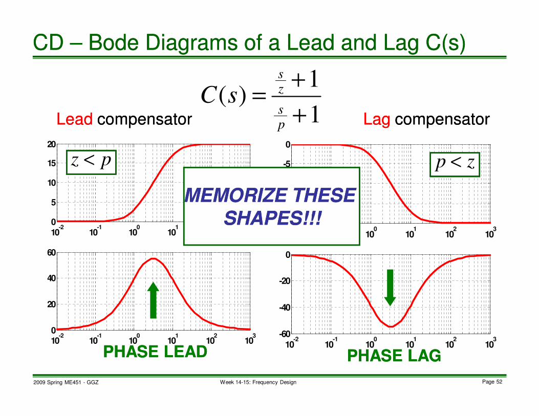
• Bode plot of a series connection G1(s)G2(s) is the addition of
each Bode plot of G1 and G2.
– Gain
– Phase
• We use this property to design C(s) so that G(s)C(s) has a
“desired” shape of Bode plot.
CD CD –– Advantages of Body DiagramAdvantages of Body Diagram
)(log20)(log20)()(log202101102110
ωωωω jGjGjGjG +=
)()()()(1121
ωωωω jGjGjGjG ∠+∠=∠

2009 Spring ME451 - GGZ Page 49Week 14-15: Frequency Design
• We use simple controllers for shaping.
– Gain
– Lead and lag compensators
CD CD –– Simple ControllersSimple Controllers
noisenoiseStable PlantStable PlantControllerController
)(ty)(tr)(sG)(sC
)(tn
)(tddisturbancedisturbance
KsC =)(
1
1
poly.)order -(1st
poly.)order -(1st)(
+
+==
ps
zs
sC
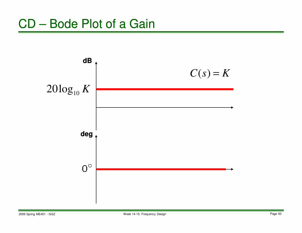
2009 Spring ME451 - GGZ Page 50Week 14-15: Frequency Design
dBdB
degdeg
CD CD –– Bode Plot of a GainBode Plot of a Gain
KsC =)(
K10
log20

2009 Spring ME451 - GGZ Page 51Week 14-15: Frequency Design
10-2
10-1
100
101
102
103
-100
-50
0
50
100
10-2
10-1
100
101
102
103
-180
-160
-140
-120
-100
In case of In case of K K > 1,> 1,
�� Gain increases Gain increases
uniformly, but phase does uniformly, but phase does
not change.not change.
�� Typically, Typically,
�� (Steady state) (Steady state) LL(0)(0)
�� (Speed) (Speed) ωωgg
�� (Stability & (Stability &
overshoot) PMovershoot) PM PMPM
CD CD –– Effect of a Gain C(s) of L(s) Effect of a Gain C(s) of L(s)
)0()( >= KsC
)(10)( sGsL =
)25(
2500)(
+=
sssG
2009 Spring ME451 - GGZ Page 52Week 14-15: Frequency Design
10-2
10-1
100
101
102
103
-20
-15
-10
-5
0
10-2
10-1
100
101
102
103
-60
-40
-20
0
10-2
10-1
100
101
102
103
0
5
10
15
20
10-2
10-1
100
101
102
103
0
20
40
60
LeadLead compensatorcompensator LagLag compensatorcompensator
PHASE LEADPHASE LEAD PHASE LAGPHASE LAG
MEMORIZE THESE MEMORIZE THESE SHAPES!!!SHAPES!!!
CD CD –– Bode Diagrams of a Lead and Lag C(s)Bode Diagrams of a Lead and Lag C(s)
pz <
1
1)(
+
+=
ps
zs
sC
zp <
2009 Spring ME451 - GGZ Page 53Week 14-15: Frequency Design
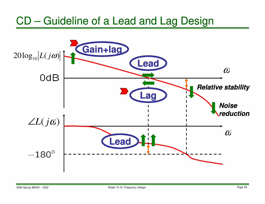
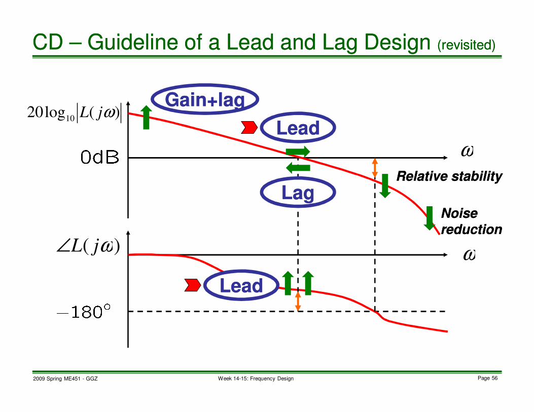
Noise Noise
reductionreduction
Relative stabilityRelative stability
Gain+lagGain+lag
LeadLead
LagLag
LeadLead
CD CD –– Guideline of a Lead and Lag DesignGuideline of a Lead and Lag Design
)( ωjL∠
)(log2010
ωjL
ω
ω

2009 Spring ME451 - GGZ Page 54Week 14-15: Frequency Design
Destabilizing effectDestabilizing effect
•• Decreasing Decreasing ωωωωωωωωgg
Select z much (at least 1 Select z much (at least 1
decade) less than decade) less than ωωgg
10-2
10-1
100
101
102
103
-20
-15
-10
-5
0
10-2
10-1
100
101
102
103
-60
-40
-20
0
CD CD –– Effect of a Lag C(s) on L(s) Effect of a Lag C(s) on L(s)
p
z10
log20

2009 Spring ME451 - GGZ Page 55Week 14-15: Frequency Design
30/1
3/1
1
110)(
s
s
LagsC
+
+=
10-2
10-1
100
101
102
103
-100
-50
0
50
100
10-2
10-1
100
101
102
103
-180
-160
-140
-120
-100
PM: 28 deg at PM: 28 deg at
ωωgg=47 rad/s=47 rad/s
PMPMPM: 27 deg at PM: 27 deg at
ωωgg=47 rad/s=47 rad/s
CD CD –– Lag + Gain C(s) DesignLag + Gain C(s) Design
)(sG)25(
2500)(
+=
sssG
)()( sCsGLag
)(sG
)()( sCsGLag
2009 Spring ME451 - GGZ Page 56Week 14-15: Frequency Design
Noise Noise
reductionreduction
Relative stabilityRelative stability
Gain+lagGain+lag
LeadLead
LagLag
LeadLead
CD CD –– Guideline of a Lead and Lag Design Guideline of a Lead and Lag Design (revisited)(revisited)
)( ωjL∠
)(log2010
ωjL
ω
ω

2009 Spring ME451 - GGZ Page 57Week 14-15: Frequency Design
10-2
10-1
100
101
102
103
0
5
10
15
20
10-2
10-1
100
101
102
103
0
20
40
60
Stabilizing effectStabilizing effect
Increasing Increasing ωωωωωωωωgg
Select z&p around Select z&p around ωωgg
CD CD –– Effect of a Lead C(s) on L(s) Effect of a Lead C(s) on L(s)

2009 Spring ME451 - GGZ Page 58Week 14-15: Frequency Design
101
102
103
-60
-40
-20
0
20
101
102
103
-180
-160
-140
-120
-100
PM: 28 deg at PM: 28 deg at
ωωgg=47 rad/s=47 rad/s
PMPMPM: 47 deg at PM: 47 deg at
ωωgg=60 rad/s=60 rad/s
CD CD –– Example of a Lead DesignExample of a Lead Design
)(sG
)()( sCsGLead
)()( sCsGLead
)(sG
1.94
21.38
1
1)(
s
s
LeadsC
+
+=
)25(
2500)(
+=
sssG

2009 Spring ME451 - GGZ Page 59Week 14-15: Frequency Design
10-2
10-1
100
101
102
103
0
5
10
15
20
10-2
10-1
100
101
102
103
-60
-40
-20
0
20
40
CD CD –– LeadLead--Lag Compensator Lag Compensator
321321Lead
s
s
LagGain
s
s
sC1.94
21.38
30/1
3/1
1
1
1
110)(
+
+⋅
+
+⋅=
+

2009 Spring ME451 - GGZ Page 60Week 14-15: Frequency Design
10-2
10-1
100
101
102
103
-100
-50
0
50
100
10-2
10-1
100
101
102
103
-180
-160
-140
-120
-100
PM: 28 deg at PM: 28 deg at
ωωg g = 47 rad/s= 47 rad/s
PMPMPM: 47 deg at PM: 47 deg at
ωωg g = 60 rad/s= 60 rad/s
CD CD –– Example of a LeadExample of a Lead--Lag DesignLag Design
)()( sCsG
)(sG
)(sG
)()( sCsG
)()()( sCsCsCLagLead
=
)25(
2500)(
+=
sssG
2009 Spring ME451 - GGZ Page 61Week 14-15: Frequency Design
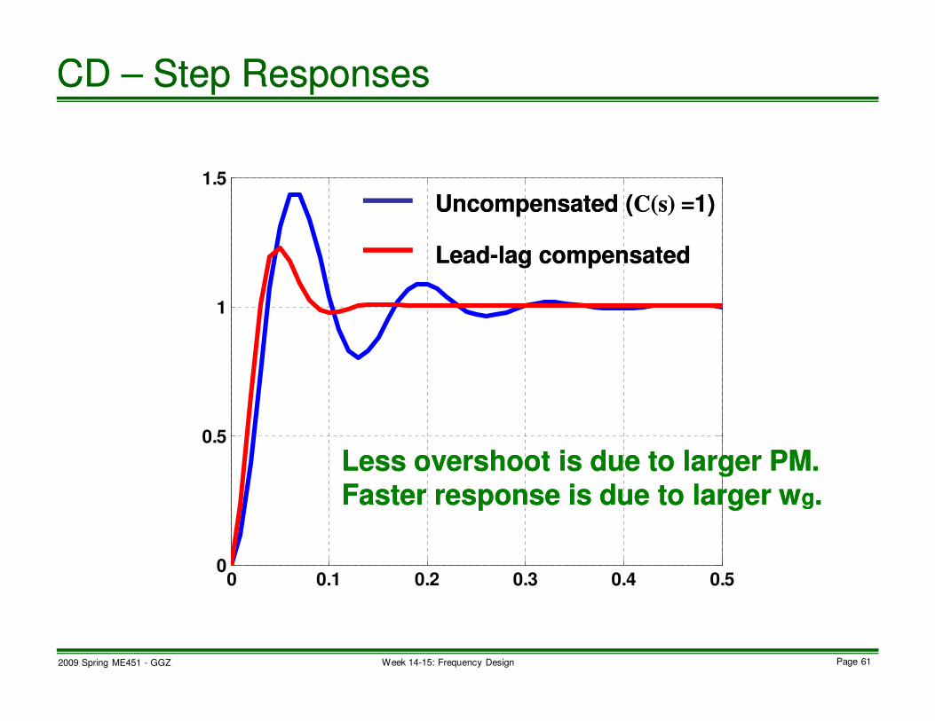
0 0.1 0.2 0.3 0.4 0.50
0.5
1
1.5
Uncompensated (Uncompensated (C(s) =C(s) =1)1)
LeadLead--lag compensatedlag compensated
Less overshoot is due to larger PM.Less overshoot is due to larger PM.
Faster response is due to larger wFaster response is due to larger wgg. .
CD CD –– Step ResponsesStep Responses

2009 Spring ME451 - GGZ Page 62Week 14-15: Frequency Design
• Frequency shaping (Loop shaping) on Bode plot
• Effect of lead, lag, and lead-lag compensators
• Qualitative explanation
• In actual design, one needs to use Matlab.
• Next, more detail about
– Lag design
– Lead design
CD CD –– Loop Shaping SummaryLoop Shaping Summary

2009 Spring ME451 - GGZ Page 63Week 14-15: Frequency Design
SteadySteady--state accuracystate accuracy
SensitivitySensitivity
Disturbance rejectionDisturbance rejection
Noise Noise
reductionreduction
TransientTransient
Response speedResponse speed
Transient Transient
OvershootOvershootRelative stabilityRelative stability
Relative stabilityRelative stabilityNoise reductionNoise reduction
• Next, frequency shaping (loop shaping) design
CD CD –– SummarySummary
)( ωjL∠
)(log2010
ωjL
ω
ω
ω

2009 Spring ME451 - GGZ Page 64Week 14-15: Frequency Design
CD CD –– Body Diagram of a Lead/Lag C(s) (Review)Body Diagram of a Lead/Lag C(s) (Review)
10-2
10-1
100
101
102
103
-20
-15
-10
-5
0
10-2
10-1
100
101
102
103
-60
-40
-20
0
10-2
10-1
100
101
102
103
0
5
10
15
20
10-2
10-1
100
101
102
103
0
20
40
60
LeadLead compensatorcompensator LagLag compensatorcompensator
PHASE LEADPHASE LEAD PHASE LAGPHASE LAG
MEMORIZE THESE MEMORIZE THESE SHAPES!!!SHAPES!!!
pz <
1
1)(
+
+=
ps
zs
sC
zp <

2009 Spring ME451 - GGZ Page 65Week 14-15: Frequency Design
dBdB +20+20
degdeg+45+45
dBdB
--2020
degdeg
--4545
Lead (z < p)Lead (z < p)
Lag (p < z)Lag (p < z)
dBdB+20+20
degdeg
+45+45
dBdB
--2020
degdeg
--4545
--4545 +45+45
CD CD –– StraightStraight--Line ApproximationsLine Approximations
1
1)(
+
+=
ps
zs
sG
1)( +=z
ssG
1
1)(
+=
ps
sG
2009 Spring ME451 - GGZ Page 66Week 14-15: Frequency Design
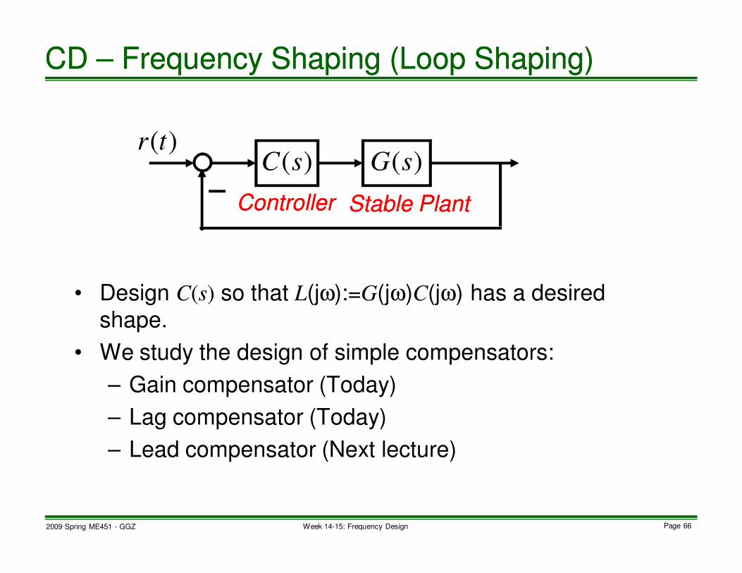
• Design C(s) so that L(jω):=G(jω)C(jω) has a desired
shape.
• We study the design of simple compensators:
– Gain compensator (Today)
– Lag compensator (Today)
– Lead compensator (Next lecture)
CD CD –– Frequency Shaping (Loop Shaping)Frequency Shaping (Loop Shaping)
Stable PlantStable PlantControllerController
)(tr)(sG)(sC

2009 Spring ME451 - GGZ Page 67Week 14-15: Frequency Design
Noise Noise
reductionreduction
Relative stabilityRelative stability
Gain+lagGain+lag
LeadLead
LagLag
LeadLead
CD CD –– Guideline of LeadGuideline of Lead--Lag Design (Review)Lag Design (Review)
)( ωjL∠
)(log2010
ωjL
ω
ω

2009 Spring ME451 - GGZ Page 68Week 14-15: Frequency Design
• Consider a system
• Analysis for C(s) = 1
– Stable
– PM at least 12 deg
– GM at least 3.5 dBThese values are too These values are too
small for good small for good
transient response!transient response!
10-2
10-1
100
101
102
-100
-50
0
50
10-2
10-1
100
101
102
-250
-200
-150
-100
CD CD –– An Example (LeadAn Example (Lead--Lag Design)Lag Design)
Stable PlantStable PlantControllerController
)(tr)(sG)(sC
)(ty
)2)(1(
4)(
++=
ssssG

2009 Spring ME451 - GGZ Page 69Week 14-15: Frequency Design
• PM is specified to be 50 deg.
• In this example, to increase PM by gain compensation,
we need to lower the gain curve.
CD CD –– Gain Margin Compensation Gain Margin Compensation (Example (2))(Example (2))

2009 Spring ME451 - GGZ Page 70Week 14-15: Frequency Design
10-2
10-1
100
101
102
-100
-50
0
50
10-2
10-1
100
101
102
-250
-200
-150
-100Uncompensated (C(s)=1)Uncompensated (C(s)=1)
Gain compensatedGain compensated
Low freq. gain Low freq. gain
decreases.decreases.
CD CD –– Bode Diagram for C(s) = 0.286 Bode Diagram for C(s) = 0.286 (Example (3))(Example (3))

2009 Spring ME451 - GGZ Page 71Week 14-15: Frequency Design
0 5 10 150
0.2
0.4
0.6
0.8
1
1.2
1.4
K=0.455 (PM=35deg)K=0.455 (PM=35deg)
K=0.286 (PM=50deg)K=0.286 (PM=50deg)
K=0.158 (PM=65deg)K=0.158 (PM=65deg)
CD CD –– Step Responses Step Responses (Example (4))(Example (4))
2009 Spring ME451 - GGZ Page 72Week 14-15: Frequency Design
dBdB
degdeg
--4545
--2020
10-2
10-1
100
101
102
103
-20
-15
-10
-5
0
10-2
10-1
100
101
102
103
-60
-40
-20
0
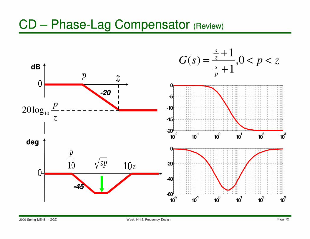
CD CD –– PhasePhase--Lag Compensator Lag Compensator (Review)(Review)
zpsGps
zs
<<+
+= 0,
1
1)(
z
p10log20
2009 Spring ME451 - GGZ Page 73Week 14-15: Frequency Design
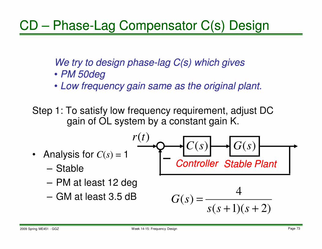
Step 1: To satisfy low frequency requirement, adjust DC gain of OL system by a constant gain K.
• Analysis for C(s) = 1
– Stable
– PM at least 12 deg
– GM at least 3.5 dB
We try to design phaseWe try to design phase--lag C(s) which giveslag C(s) which gives
•• PM 50degPM 50deg
•• Low frequency gain same as the original plant.Low frequency gain same as the original plant.
CD CD –– PhasePhase--Lag Compensator C(s) DesignLag Compensator C(s) Design
Stable PlantStable PlantControllerController
)(tr)(sG)(sC
)2)(1(
4)(
++=
ssssG
2009 Spring ME451 - GGZ Page 74Week 14-15: Frequency Design
10-2
10-1
100
101
102
-100
-50
0
50
10-2
10-1
100
101
102
-250
-200
-150
-100
OKOK
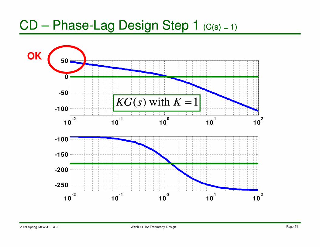
CD CD –– PhasePhase--Lag Design Step 1 Lag Design Step 1 (C(s) = 1)(C(s) = 1)
1 with )( =KsKG

2009 Spring ME451 - GGZ Page 75Week 14-15: Frequency Design
Step 2: Find the frequency ωg (which will become gain
crossover frequency after compensation) where
In this example,
Note: The reason of +5 deg is explained later.
CD CD –– PhasePhase--Lag Design Step 2 Lag Design Step 2 (C(s) = 1)(C(s) = 1)
4.0=g
ω
PM required : ,5180)(m
o
m
o
gjG φφω ++−=∠
{oooo
g
m
jG 125550180)( −=++−=∠φ
ω

2009 Spring ME451 - GGZ Page 76Week 14-15: Frequency Design
10-2
10-1
100
101
102
-100
-50
0
50
10-2
10-1
100
101
102
-250
-200
-150
-100
PM=55PM=55
CD CD –– PhasePhase--Lag Design Step 2 Lag Design Step 2 (C(s) = 1)(C(s) = 1)
)(sKG
gω

2009 Spring ME451 - GGZ Page 77Week 14-15: Frequency Design
Step 3:
dBdB
--2020
degdeg
--4545
For small phase lag at For small phase lag at ωωgg
For setting new gain crossover at For setting new gain crossover at ωωgg
CD CD –– PhasePhase--Lag Design Step 3 Lag Design Step 3 (C(s) = 1)(C(s) = 1)
)55.4
04.0(
)(
1.0==
g
g
jKGp
ω
ω
)04.0(1.0 ==g
z ω
)(
1log20log20
1010
gjKGz
p
ω=

2009 Spring ME451 - GGZ Page 78Week 14-15: Frequency Design
10-2
10-1
100
101
102
-100
-50
0
50
10-2
10-1
100
101
102
-250
-200
-150
-100
PM=50PM=50
CD CD –– PhasePhase--Lag Design Step 3 Lag Design Step 3 (C(s) = C(C(s) = Claglag(s))(s))
)(sKG
1
1)(
0088.0
04.0
+
+=
s
s
LagsC
)()( sCsKGLag
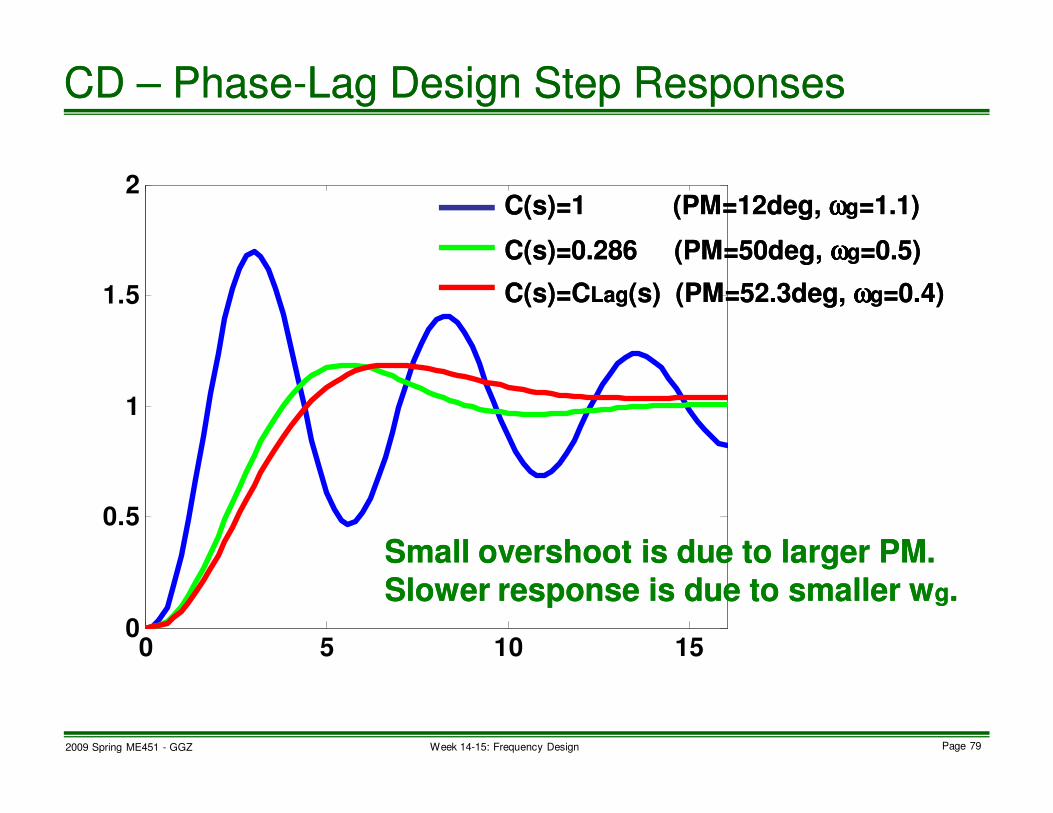
2009 Spring ME451 - GGZ Page 79Week 14-15: Frequency Design
0 5 10 150
0.5
1
1.5
2
C(s)=0.286 (PM=50deg, C(s)=0.286 (PM=50deg, ωωωωωωωωgg=0.5)=0.5)
C(s)=CC(s)=CLagLag(s) (PM=52.3deg, (s) (PM=52.3deg, ωωωωωωωωgg=0.4)=0.4)
Small overshoot is due to larger PM.Small overshoot is due to larger PM.
Slower response is due to smaller wSlower response is due to smaller wgg. .
C(s)=1C(s)=1 (PM=12deg, (PM=12deg, ωωωωωωωωgg=1.1)=1.1)
CD CD –– PhasePhase--Lag Design Step ResponsesLag Design Step Responses
2009 Spring ME451 - GGZ Page 80Week 14-15: Frequency Design
• Gain controller design in Bode plot
– Gain changes uniformly over frequencies.
– Phase does not change.
• Lag compensator design in Bode plot
– Lag compensator can be used for
• Improving PM by maintaining low freq. gain, or
• Improving low freq. gain by maintaining PM
• Low freq. gain determines steady state error, disturbance
rejection, while PM does overshoot.
• Next, lead compensator design
CD CD –– PhasePhase--Lag Design SummaryLag Design Summary

2009 Spring ME451 - GGZ Page 81Week 14-15: Frequency Design
• What is problematic?
– Nyquist stability criterion says that, for closed-loop
stability, Nyquist plot of open-loop system must
encircle -1 point.
– It is hard to translate this condition into Bode plot.
• To use FR technique…
UnstableUnstableControllerController
Stabilize first!Stabilize first!
CD CD –– If G(s) has OL RHP PolesIf G(s) has OL RHP Poles
)(sG)(sC
)(sH

2009 Spring ME451 - GGZ Page 82Week 14-15: Frequency Design
1. Select z near uncompensated ωg.
In the example, ωg = 1.14. So, select, for example, z = 1.
2. Select p > z by trial-and-error.
3. Check PM and settling time. If not satisfactory, move the
pole p. If moving pole does not give the desired results,
try to move the zero z.
CD CD –– PhasePhase--Lead Design ProcedureLead Design Procedure

2009 Spring ME451 - GGZ Page 83Week 14-15: Frequency Design
10-2
10-1
100
101
102
-100
-50
0
50
10-2
10-1
100
101
102
-250
-200
-150
-100
PM=50PM=50
CD CD –– PhasePhase--Lead Design ExampleLead Design Example
)(sG
1
1)(
50+
+=
sLead
ssC
)()( sCsGLead
57.1=g
ω

2009 Spring ME451 - GGZ Page 84Week 14-15: Frequency Design
0 5 10 150
0.5
1
1.5
2C(s)=0.286 (PM=50deg, C(s)=0.286 (PM=50deg, ωωωωωωωωgg=0.5)=0.5)
C(s)=CC(s)=CLagLag(s) (PM=52.3deg, (s) (PM=52.3deg, ωωωωωωωωgg=0.4)=0.4)
C(s)=1C(s)=1 (PM=12deg, (PM=12deg, ωωωωωωωωgg=1.1)=1.1)
C(s)=CC(s)=CLeadLead(s) (PM=50deg, (s) (PM=50deg, ωωωωωωωωgg=1.6)=1.6)
Faster response is due to larger wFaster response is due to larger wgg..
(Compare crossover frequencies.) (Compare crossover frequencies.)
CD CD –– PhasePhase--Lead Design Step ResponsesLead Design Step Responses

2009 Spring ME451 - GGZ Page 85Week 14-15: Frequency Design
69 69.2 69.4 69.6 69.8 7067
67.5
68
68.5
69
69.5
70
C(s)=0.286 (Kv=0.572)C(s)=0.286 (Kv=0.572)
Ramp referenceRamp reference
C(s)=CC(s)=CLagLag(s) (Kv=2)(s) (Kv=2)
C(s)=1C(s)=1 (Kv=2)(Kv=2)
C(s)=CC(s)=CLeadLead(s) (Kv=2)(s) (Kv=2)
CD CD –– PhasePhase--Lead Design Ramp ResponsesLead Design Ramp Responses

2009 Spring ME451 - GGZ Page 86Week 14-15: Frequency Design
10-2
10-1
100
101
102
-100
-50
0
50
10-2
10-1
100
101
102
-250
-200
-150
-100
We recover the gain loss We recover the gain loss
at gain crossover freq.at gain crossover freq.
by adding a gain.by adding a gain.
CD CD –– Phase LeadPhase Lead--Lag Design Example (1)Lag Design Example (1)
)(sG
)()( sCsGLead
)()()( sCsCsGLagLead

2009 Spring ME451 - GGZ Page 87Week 14-15: Frequency Design
10-2
10-1
100
101
102
-100
-50
0
50
10-2
10-1
100
101
102
-250
-200
-150
-100
PM=51PM=51
IncreasedIncreased
CD CD –– Phase LeadPhase Lead--Lag Design Example (2)Lag Design Example (2)
)(sG
)()(4)( sCsCsCLagLeadLL
=
)()( sCsGLL
43.1=g
ω

2009 Spring ME451 - GGZ Page 88Week 14-15: Frequency Design
0 5 10 150
0.5
1
1.5
2
C(s)=0.286C(s)=0.286
C(s)=CC(s)=CLagLag(s)(s)
C(s)=1C(s)=1
C(s)=4CC(s)=4CLeadLead(s)C(s)CLagLag(s)(s)
CD CD –– Phase LeadPhase Lead--Lag Design Step ResponsesLag Design Step Responses

2009 Spring ME451 - GGZ Page 89Week 14-15: Frequency Design
• Lead compensator can be used for improving
• Gain crossover frequency
• Phase margin
by maintaining low frequency gain,
• Lead-lag compensator can improve
– Transient (ωg for speed, PM for overshoot)
– Steady state (low frequency gain for error constant)
• Next, case studies
– Antenna azimuth position control
– Hard disk drive control
CD CD –– LeadLead--Lag Compensator SummaryLag Compensator Summary

2009 Spring ME451 - GGZ Page 90Week 14-15: Frequency Design
• Characteristics
CD CD –– Design Example Design Example –– PD Controller (1)PD Controller (1)
KKKbKbsKsCDp
==+= , where),()(
When K = 1/b, we have
dB20
o90
b1.0 b10b
o0
dB0
φ
ω
ωφ
tan
,tan1
=
=−
b
b

2009 Spring ME451 - GGZ Page 91Week 14-15: Frequency Design
CD CD –– Design Example Design Example –– PD Controller (2)PD Controller (2)
)3)(1(
21)(
++=
ssssG
A Design Example (9.9)
71.23.5tan40
8
tan)(
81
===o
DsT φω
)(sG)(sC-
Design Target: %)2( sec)( 5.3 ,40 : ≤=sD
TPMoφ
Select crossover frequency (see text book page 373, Eq. 9-33):
0.3Select =cω
Bode Diagram (Blue Line next page):
)1)(1(
7)(
3++
=sss
sG
Step 1:
Step 2:

2009 Spring ME451 - GGZ Page 92Week 14-15: Frequency Design
CD CD –– Design Example Design Example –– PD Controller (3)PD Controller (3)
-100
-50
0
50
Ma
gnitu
de
(d
B)
10-1
100
101
102
-270
-225
-180
-135
-90
Pha
se
(d
eg)
Bode Diagram
Frequency (rad/sec)
Open Loop Bode Diagram (Blue Line):
3=c
ω
o8.206−o8.66
Phase Error
dB01.7Gain Error

2009 Spring ME451 - GGZ Page 93Week 14-15: Frequency Design
CD CD –– Design Example Design Example –– PD Controller (4)PD Controller (4)
ooo 8.661808.206 =+−=DMAX
Ph φ
Find Phase Margin at ωc:
284.1tan66.8
3
tan===
oφ
ωCb
8.206)( o−=COL
PM ω
PD Controller Compensate Phase to have desired PM:
444 3444 21Controller
)284.1()(
PD
sKsC +=
Step 3:
Step 4:

2009 Spring ME451 - GGZ Page 94Week 14-15: Frequency Design
CD CD –– Design Example Design Example –– PD Controller (5)PD Controller (5)
dBK 01.7log2010
−=
Plot Bode Diagram (Mag. only – Green) with K = 1.
And then find gain error:
2.242)()()( ==CCCGN
jLjCERR ωωω
Calculate the controller gain K:
)284.1(446.0)( += ssC
Step 5:
Step 6:
dB 7.01)( =CGN
ERR ω
)()( sLsC
446.010 20
01.7
==
−
K
Resulting PD controller:

2009 Spring ME451 - GGZ Page 95Week 14-15: Frequency Design
CD CD –– Design Example Design Example –– PD Controller (6)PD Controller (6)
Plot Bode Diagram (Red) with K = 0.446 results
o4.39=PM
3=Cω
)()( sLsC
)180 than lessdelay (Phase o∞=GM

2009 Spring ME451 - GGZ Page 96Week 14-15: Frequency Design
CD CD –– Design Example Design Example –– PD Controller (7)PD Controller (7)
)3)(1(
21)(
++=
ssssC
Design by Root Locus:
4.0100
40
100===
oo
Dφ
ς
)(sL)(sC-
Design Target: %)2( sec)( 5.3 ,40 : ≤=sD
TPMoφ
Select desired damp coefficient (text book page 328, Eq. 8-50):
Select desired frequency ωn:
5.34
=n
ςω
Step 1:
Step 2:
86.25.34.0
4=
⋅=
nω 86.23Select ≥=
nω
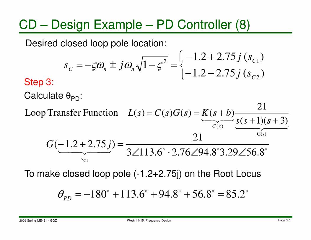
2009 Spring ME451 - GGZ Page 97Week 14-15: Frequency Design
CD CD –– Design Example Design Example –– PD Controller (8)PD Controller (8)
−−
+−=−±−=
)( 75.22.1
)( 75.22.11
2
12
C
C
nnCsj
sjjs ςωςω
Desired closed loop pole location:
ooo4434421 8.5629.38.9476.26.1133
21)75.22.1(
1
∠∠⋅∠=+−
Cs
jG
)3)(1(
21)()()()( Function Transfer Loop
G(s)
)( 44 344 2143421 +++==
sssbsKsGsCsL
sC
Calculate θPD:
To make closed loop pole (-1.2+2.75j) on the Root Locus
Step 3:
ooooo 2.858.568.946.113180 =+++−=PD
θ

2009 Spring ME451 - GGZ Page 98Week 14-15: Frequency Design
CD CD –– Design Example Design Example –– PD Controller (9)PD Controller (9)
43.12.12.85tan
75.2
tan
12
=+=+−
=on
PD
nb ςωθ
ςω
47.076.221
29.376.23=
⋅
⋅⋅=K
o
44344212.8576.275.22.1
1
∠=++− bj
Cs
Calculate b:
To make closed loop pole (-1.2+2.75j) on the Root Locus
Step 4:
129.376.23
2176.2)()()(
)(
)(
111
1
1
=⋅⋅
⋅==4434421
321
C
C
sG
sC
CCCKsGsCsL
Step 5:
Calculate K:
)43.1(47.0)( += ssC

2009 Spring ME451 - GGZ Page 99Week 14-15: Frequency Design
CD CD –– Design Example Design Example –– PD Controller (10)PD Controller (10)
Bode Diagram Design
Root Locus Design
)43.1(47.0)( += ssC
)284.1(446.0)( += ssC
-3 -2.5 -2 -1.5 -1 -0.5 0-5
-4
-3
-2
-1
0
1
2
3
4
5
0.84
0.050.110.170.240.340.46
0.62
0.84
1
2
3
4
5
1
2
3
4
5
0.050.110.170.240.340.46
0.62
Root Locus
Real Axis
Imagin
ary
Axi
s
-3 -2.5 -2 -1.5 -1 -0.5 0-5
-4
-3
-2
-1
0
1
2
3
4
5
0.84
0.050.110.170.240.340.46
0.62
0.84
1
2
3
4
5
1
2
3
4
5
0.050.110.170.240.340.46
0.62
Root Locus
Real Axis
Imagin
ary
Axi
s

2009 Spring ME451 - GGZ Page
100Week 14-15: Frequency Design
• Characteristics
CD CD –– Design Example Design Example –– Lead Controller (1)Lead Controller (1)
1 controller lead afor ,1
1)( >
+
+= α
τ
ατ
s
sKsC
When K = 1, we have the following Bode plot
α10
log20
o90
ατ
1
o0
dB0
1
1sin
+
−=
α
αφ
m
α10
log10
τ
1
τα
1
mφ
m
m
φ
φα
sin1
sin1
−
+=
Key Formula:

2009 Spring ME451 - GGZ Page
101Week 14-15: Frequency Design
CD CD –– Design Example Design Example –– Lead Controller (2)Lead Controller (2)
)2(
1)(
+=
sssG
A Design Example – Lead Controller
error SS %5
)(sG)(sC-
Design Target: %5error Ramp StateSteady ,45 : ≤= o
DPM φ
Determine control gain K by steady state error requirement:
2
1)()(lim20
05.0
1
0KsGssCK
sv
====→
Step 1:
Controller to be designed: s
sKsC
τ
ατ
+
+=
1
1)(
40=K

2009 Spring ME451 - GGZ Page
102Week 14-15: Frequency Design
CD CD –– Design Example Design Example –– Lead Controller (3)Lead Controller (3)
Draw Bode diagram of )1s(
20
)2(
40)(
2s +
=+
=ss
sG
Step 2:
dB40
OLC _ω
o90−
dB0
dB20
202
o18=OL
PM
dB20−
o180−
85.4 5.14
dB8.4−m
ω

2009 Spring ME451 - GGZ Page
103Week 14-15: Frequency Design
CD CD –– Design Example Design Example –– Lead Controller (4)Lead Controller (4)
Calculate α:
To get PM = 45° we target φm=30°, leading to PM =48°:
o30=m
φ
Step 3:
Step 4:
3-1
1
30sin1
30sin1
21
21
=+
=−
+=
o
o
α
)()( sLsC
44444 344444 21rCompensatoLeadtodueIncreaseGain
dB
10108.43log10log10 ==α
Find τ:
To find τ, we need to find ωm such that:
dBjGm
8.4log10)(log201010
−=−= αω

2009 Spring ME451 - GGZ Page
104Week 14-15: Frequency Design
CD CD –– Design Example Design Example –– Lead Controller (5)Lead Controller (5)
From Bode diagram, we have
0687.034.8
1==τ
85.40687.03
11=
⋅==
ατz
rad/s 4.8=m
ω
s
ssC
s
s
0687.01
2061.0140
)1(
)1(40)(
5.14
85.4
+
+=
+
+=
Therefore,
Then
8.41
==ατ
ωm
5.140687.0
11===
τp

2009 Spring ME451 - GGZ Page
105Week 14-15: Frequency Design
CD CD –– Design Example Design Example –– Lead Controller Lead Controller (6)(6)
-100
-50
0
50M
agnitu
de (
dB
)
10-1
100
101
102
103
-180
-135
-90
Phase (
deg)
Bode Diagram
Frequency (rad/sec)
PM=39.4
ωωωωc=8.4
)1)(1(
)1(20)()(
5.142
85.4
ss
s
ssGsC
++
+=