Embed Size (px)
Citation preview

Classical Decomposition Model Revisited: I
• recall classical decomposition model for time series Yt, namely,
Yt = mt + st + Wt, (∗)where mt is trend; st is periodic with known period s (i.e.,st−s = st for all t ∈ Z) satisfying
∑sj=1 sj = 0; and Wt is a
stationary process with zero mean
•mt & st often taken to be deterministic
• as we have seen, SARIMA processes can model stochastic st,but can also handle deterministic mt & st through differencing
• differencing to eliminate deterministic mt and/or st can leadto undesirable overdifferencing of Wt
• alternative approach: regard (∗) to be a regression model withstationary errors
BD: 20, CC: 27, 30, 32, SS: 45 XVII–1

Classical Decomposition Model Revisited: II
• will now consider a linear regression approach in which mtand/or st depend linearly on a small number of parameters
• note: nonparametric regression another option (expands uponideas discussed earlier of using filtering operations to extracttrends – see overhead III–25 and discussion following it)
BD: 20, CC: 27, 30, 32, SS: 45 XVII–2
Regression with Stationary Errors: I
• in context of time series analysis, standard linear regressionmodel would take form
Y = Xβ +Z,
where
− Y = [Y1, . . . , Yn]′ is vector containing series;
−X is an n× k design matrix whose tth row x′t has values ofexplanatory variables for Yt;
− β = [β1, . . . , βk]′ is vector of regression coefficients; and
− Z = [Z1, . . . , Zn]′ is vector of WN(0, σ2) RVs
• example: Yt = β1 +β2t+Zt, for which tth row of n× 2 designmatrix X would be x′t = [1, t]
• second example: Yt = β1 + β2 cos (2πft) + β3 sin (2πft) + Zt
BD: 184, CC: 30, SS: 47 XVII–3

Regression with Stationary Errors: II
• ordinary least squares (OLS) estimator of β is vector βOLSminimizing sum of squared errors:
S(β) =
n∑t=1
(Yt − x′tβ)2 = (Y −Xβ)′(Y −Xβ)
• βOLS is solution to so-called normal equations:
X ′Xβ = X ′Y and hence βOLS = (X ′X)−1X ′Y
if X ′X has full rank
• βOLS is best linear unbiased estimator of β (best in that, if βis any other unbiased estimator, then var{c′βOLS} ≤ var{c′β}for any vector c of constants)
• covariance matrix for βOLS given by σ2(X ′X)−1
BD: 184, SS: 47 XVII–4
Regression with Stationary Errors: III
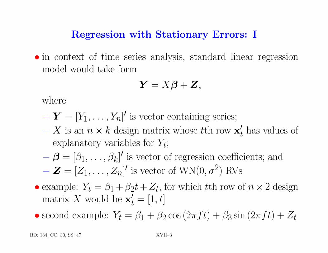
• for time series, uncorrelated errors Z are usually unrealistic
• often a more realistic model is
Y = Xβ +W ,
where W contains RVs from a stationary process with zeromean, an example being a causal ARMA(p, q) process:
φ(B)Wt = θ(B)Zt, {Zt} ∼WN(0, σ2)
• under this alternative model, βOLS is still an unbiased estimatorof β, but best linear unbiased estimator is generalized leastsquares (GLS) estimator
• in the full rank case, this estimator takes the form
βGLS = (X ′Γ−1n X)−1X ′Γ−1
n Y ,
where Γn is covariance matrix for W
BD: 184–185 XVII–5

Regression with Stationary Errors: IV
• βGLS is minimizer of weighted sum of squares:
S(β) = (Y −Xβ)′Γ−1n (Y −Xβ)
• to motivate this estimator, recall innovations representation forstationary process says that W = CnU , where U = W − W(U are the innovations, and W are 1-step-ahead predictions)
• recall that, if V has covariance matrix Σn, then covariancematrix for AV is AΣnA
′
• sinceU has diagonal covariance matrixDn, get Γn = CnDnC′n
• let D−1/2n be diagonal matrix such that D
−1/2n D
−1/2n = D−1
n
• covariance matrix for D−1/2n C−1
n W is identity matrix In since
D−1/2n C−1
n Γn(C−1n )′D−1/2
n = D−1/2n C−1
n CnDnC′n(C−1
n )′D−1/2n = In
BD: 185–186 XVII–6

Regression with Stationary Errors: V
• returning now to model Y = Xβ+W , multiplication of both
sides by D−1/2n C−1
n yields
D−1/2n C−1
n Y = D−1/2n C−1
n Xβ + D−1/2n C−1
n W ,
which can be reexpressed as
Y = Xβ +Z, {Zt} ∼WN(0, 1)
• for this regression model, best linear unbiased estimator is
βOLS = (X ′X)−1X ′Y
= (X ′(C−1n )′D−1/2
n D−1/2n C−1
n X)−1X ′(C−1n )′D−1/2
n D−1/2n C−1
n Y
= (X ′(C−1n )′D−1
n C−1n X)−1X ′(C−1
n )′D−1n C−1
n Y
= (X ′Γ−1n X)−1X ′Γ−1
n Y = βGLS
since Γn = CnDnC′n says Γ−1
n = (C ′n)−1DnC−1n = (C−1
n )′DnC−1n
BD: 185–186 XVII–7

Regression with Stationary Errors: VI
• in principle, can use ML under a Gaussian assumption to esti-mate all parameters in model Y = Xβ+W (i.e., both β andparameters associated with, e.g., ARMA model)
• in practice, following simpler (but sub-optimal) iterative schemefor parameter estimation often works well
1. compute βOLS and form residuals Yt − x′tβOLS2. fit ARMA(p,q) or other stationary model to residuals
3. using fitted model, compute βGLS and form residuals Yt −x′tβGLS
4. fit same model to residuals again
5. repeat steps 3 and 4 until parameter estimates have stabilized
BD: 185–186, SS: 144 XVII–8

1st Difference of Atomic Clock Data Revisited: I
• let’s reconsider modeling 1st difference of atomic clock data Xt,i.e., ∇Xt• 2nd difference∇2Xt well-modeled by ARMA(1,1) process (over-
heads XIII–129 to 135), with support for need for 2nd differ-encing coming from augmented Dickey–Fuller (ADF) unit roottest (overhead XIV–44)
• modeling∇Xt as a stationary fractionally differenced (FD) pro-cess proved to be questionable (overheads XVI–72 to 77)
• apparent linear increase in ∇Xt suggests exploring model oflinear trend + stationary noise more seriously (looked brieflyat this approach in context of ADF unit root test, where wefound that linear detrending obviated need for 2nd differencing– see overheads XIV–44 and 45)
XVII–9

1st Difference of Atomic Clock Time Series
0 200 400 600 800 1000
−17
0−
150
−13
0
t
x t
XVII–10
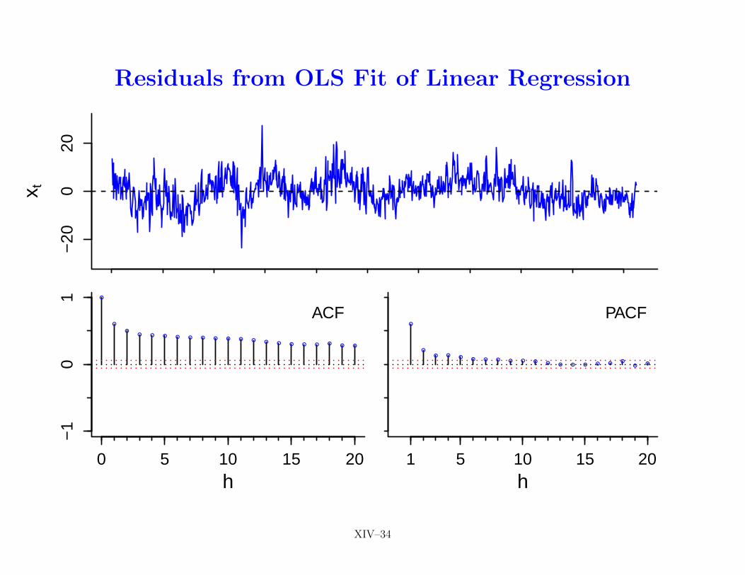
Residuals from OLS Fit of Linear Regression−
200
20
x t
●
●
●● ● ● ● ● ● ● ● ● ● ● ● ● ● ● ● ● ●
0 5 10 15 20h
−1
01
ACF●
●
● ● ●● ● ● ● ● ● ● ● ● ● ● ●
●●
●
1 5 10 15 20h
PACF
XIV–34

1st Difference of Atomic Clock Data Revisited: II
• sample ACF and PACF suggest three models for residuals:
− AR(p), with p somewhere around 7 or 8
− ARMA(p,q), with p + q small
− ARFIMA(p,δ,q), with p + q small (= 0 gives FD(δ))
• let’s consider various possibilities, using
− maximum likelihood to fit each model
− AICC to evaluate different models
• start by considering AR(p) models of orders p = 1, . . . , 20
XVIII–11

ML-Based AICC for Residuals Modeled by AR(p)
●
●
●
●
●●
●● ● ● ● ●
●●
●● ● ● ● ●
5 10 15 20
6020
6040
6060
6080
6100
6120
p (AR model order)
AIC
C
XVIII–12

1st Difference of Atomic Clock Data Revisited: III
• AR(11) best amongst AR(p) with AICC of 6020.89
• here are AICCs for ARMA(p,q) models with p + q ≤ 4
p q AICC0 1 6301.190 2 6197.770 3 6159.830 4 6135.891 1 6033.781 2 6010.361 3 6008.192 1 6007.072 2 6009.013 1 6008.98
XVIII–13

1st Difference of Atomic Clock Data Revisited: IV
• let’s compare AICC for ARMA(2,1) with ones for ARMA(p,q)models with p + q = 5
p q AICC2 1 6007.070 5 6114.911 4 6010.182 3 6010.193 2 6010.714 1 6010.01
• let’s now see if we can find an ARFIMA(p,δ,q) model that hasa better AICC than one for ARMA(2,1) model
XVIII–14

1st Difference of Atomic Clock Data Revisited: V
p δ q AICC2 0 1 6007.070 0.405 0 6015.170 0.391 1 6015.100 0.426 2 6015.450 0.430 3 6015.571 0.395 0 6015.141 0.398 1 6008.701 0.097 2 6007.302 0.417 0 6015.852 0.000 1 6007.613 0.432 0 6015.08
• conclusion: will go with ARMA(2,1) model
XVIII–15

1st Difference of Atomic Clock Data Revisited: VI
• using R function arima to fit model
∇Xt = a + bt + Wt, {Wt} ∼ ARMA(2,1),
ML estimates of model parameters a, b, φ1, φ2 and θ1 (alongwith standard errors (SEs)) are
a b φ1 φ1 θ1value −159.2759 0.0334 1.2218 −0.2432 −0.8315SE 2.0863 0.0035 0.0453 0.0412 0.0299
• estimate of σ2 is σ2 .= 20.3653; next plots show
−∇Xt & lines fitted by OLS (red) & GLS (black dashed)
− comparison of ARMA(2,1) ACF & PACF with sample ACF& PACF for ∇Xt − a− bt
− residuals Rt returned by arima and associated diagnostics
XVIII–16

1st Difference of Atomic Clock Time Series
0 200 400 600 800 1000
−17
0−
150
−13
0
t
x t
XVIII–17

Sample ACF for ∇Xt − a− bt & ARMA(2,1) ACF
●
●● ● ● ● ● ● ● ● ● ● ● ● ● ● ● ● ● ● ● ● ● ● ● ● ● ● ● ● ● ● ● ● ● ● ● ● ● ●
0 10 20 30 40
−0.
50.
00.
51.
0
h (lag)
AC
F
XVIII–18
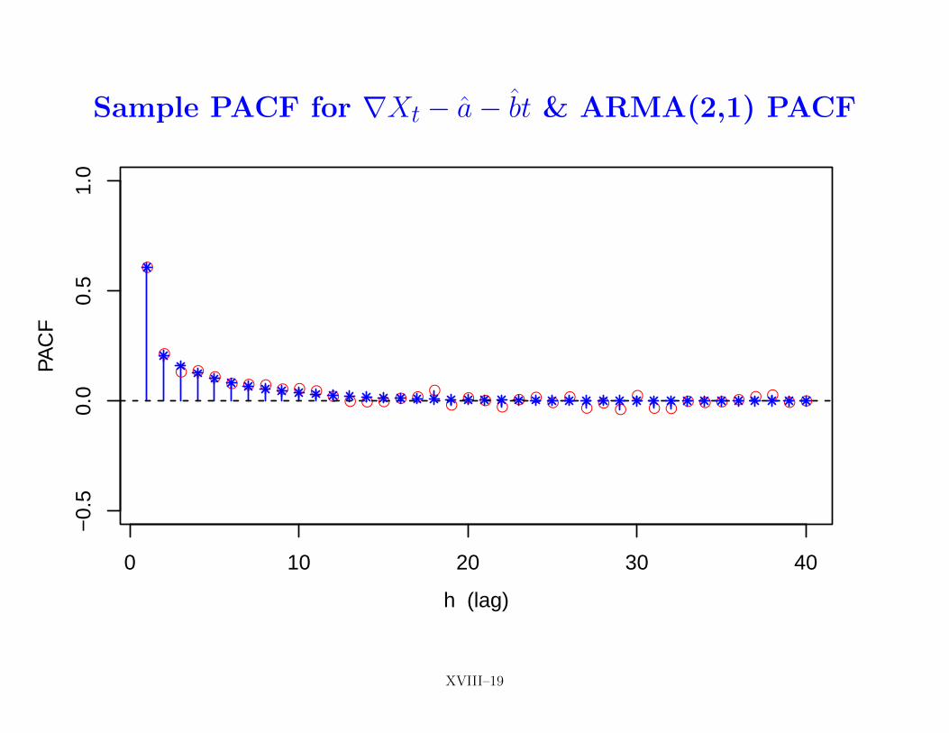
Sample PACF for ∇Xt − a− bt & ARMA(2,1) PACF
●
●
● ● ●● ● ● ● ● ● ● ● ● ● ● ●
●●
● ●●
● ● ● ●● ●
●●
● ●● ● ● ● ● ●
● ●
0 10 20 30 40
−0.
50.
00.
51.
0
h (lag)
PAC
F
XVIII–19

ARMA(2,1) Residuals Rt for Atomic Clock
0 200 400 600 800 1000
−20
−10
010
20
t
Rt
XVIII–20

Sample ACF for ARMA(2,1) Residuals Rt
●
●
●
●●
● ●● ●
●●
●
●● ●
● ●
●
●
● ●
●●
●●
●
●
●
●
●
●
●● ● ● ●
●
●
●●
0 10 20 30 40
−0.
2−
0.1
0.0
0.1
0.2
h (lag)
AC
F
XVIII–21

Sample PACF for ARMA(2,1) Residuals Rt
●
●
●
●●
● ●● ●
●●
●
●● ●
● ●
●
●
● ●
●●
●
●
●
●●
●
●
●
●
● ● ● ●●
●
●●
0 10 20 30 40
−0.
2−
0.1
0.0
0.1
0.2
h (lag)
PAC
F
XVIII–22

Portmanteau Tests of ARMA(2,1) Residuals Rt
● ● ● ● ●● ● ● ● ● ● ●
● ● ●
0 5 10 15 20
05
1015
2025
h (lag)
QLB
(h)
and
95%
qua
ntile
XVIII–23

Diagnostics Tests of ARMA(2,1) Residuals Rt
expected testtest value statistic p-value
turning point 682 708 0.054difference-sign 512 512 1.00
rank 262400 263233 0.879runs 513.2 525 0.460
AR method AICC order AIC orderYule–Walker 0 0
Burg 0 0OLS 0 4MLE 0 0
XVIII–24

Regression with Stationary Errors: VII
• cautionary note: Y ′Y 6= Y ′Y = Y ′Γ−1n Y , so portion of sum
of squares explained by transformed model cannot be relateddirectly to sum of squares for untransformed data
• assuming W in model Y = Xβ +W has covariance matrixΓn, covariance matrices for βOLS and βGLS are, respectively,
(X ′X)−1X ′ΓnX(X ′X)−1 and (X ′Γ−1n X)−1
• assuming W for ∇Xt clock data is ARMA(2,1) process, canassess standard errors (SEs) for estimated slopes
OLS GLSslope 0.03437 0.03337 (≈ 3% difference between estimates)SE 0.00358 0.00346 (≈ 3% increase for OLS over GLS)
• if assumeW is WN, SE for OLS slope estimate would be takenas 0.00064 (5× smaller than when correlation is accounted for)
XVIII–25

Harmonic Regression and CO2 Series: I
• atomic clock ∇Xt illustrates handling deterministic trend mtin model
Yt = mt + Wt
via a parametric regression approach (mt = a + bt)
• as a second example, reconsider CO2 series from Mauna Loa,Hawaii (subject of Problem 8)
• appropriate model here is full classical decomposition model:
Yt = mt + st + Wt
where mt is trend; st is seasonal component with period s = 12(i.e., st−12 = st for all t ∈ Z) satisfying
∑12j=1 sj = 0; and Wt
is a stationary process with zero mean
• for illustrative purposes, will take mt & st to be deterministic
XVIII–26

2nd Example: CO2 Series from Mauna Loa, Hawaii
1960 1970 1980 1990 2000 2010 2020
320
340
360
380
400
year
y t
III–2

Preliminary Nonparametric Estimate of Trend
1960 1970 1980 1990 2000 2010 2020
320
340
360
380
400
year
y t a
nd m
t
XVIII–27

Preliminary Detrended Series
1960 1970 1980 1990 2000 2010 2020
−4
−2
02
4
year
u t=
y t−
mt
XVIII–28

Estimated Seasonal Component
●
●
●
●
●
●
●
●
● ●
●
●
Jan Feb Mar Apr May June July Aug Sep Oct Nov Dec
−3
−2
−1
01
23
month
year
ly p
atte
rn o
f st
XVIII–29

Harmonic Regression and CO2 Series: II
• factoid: can represent any deterministic st with period 12 by
st =
6∑j=1
Aj cos (2πfjt) + Bj sin (2πfjt) =
6∑j=1
Dj cos (2πfjt + ϕj),
where fjdef= j/12 is a frequency with associated period 1/fj:
treating t momentarily as t ∈ R rather than t ∈ Z, have
cos (2πfj(t + 1fj
)) = cos (2πfjt + 2π) = cos (2πfjt)
with a similar result holding for sin (2πfjt).
• since∑12j=1 sj = 0, any eleven sj’s determine remaining twelfth
• six Aj’s and six Bj’s seem one too many, but in fact there areonly five relevant Bj’s: B6 doesn’t enter in play because
B6 sin (2πf6t) = B6 sin (2π 612t) = B6 sin (πt) = 0 for all t
XVIII–30
Harmonic Regression and CO2 Series: III
• f1 is known as the fundamental frequency, whereas f2, . . . , f6are called first, . . . , fifth harmonics
• since fj = j/12, have fj = jf1 for j = 2, . . . , 6, so harmonicsare integer multiples of fundamental frequency
• if seasonal component st slowly varying from one month tonext, can often get by with using just fundamental frequencyand a small number of harmonics:
st ≈J∑j=1
Aj cos (2πfjt) + Bj sin (2πfjt), 1 ≤ J < 6
• following plots show approximations of orders J = 1, . . . 5 toseasonal component st estimated in Problem 8 for CO2 series
XVIII–31

J = 1 Approximation to Seasonal Component
●
●
●
●
●
●
●
●
● ●
●
●
Jan Feb Mar Apr May June July Aug Sep Oct Nov Dec
−3
−2
−1
01
23
month
year
ly p
atte
rn o
f st
XVIII–32

J = 2 Approximation to Seasonal Component
●
●
●
●
●
●
●
●
● ●
●
●
Jan Feb Mar Apr May June July Aug Sep Oct Nov Dec
−3
−2
−1
01
23
month
year
ly p
atte
rn o
f st
XVIII–33

J = 3 Approximation to Seasonal Component
●
●
●
●
●
●
●
●
● ●
●
●
Jan Feb Mar Apr May June July Aug Sep Oct Nov Dec
−3
−2
−1
01
23
month
year
ly p
atte
rn o
f st
XVIII–34

J = 4 Approximation to Seasonal Component
●
●
●
●
●
●
●
●
● ●
●
●
Jan Feb Mar Apr May June July Aug Sep Oct Nov Dec
−3
−2
−1
01
23
month
year
ly p
atte
rn o
f st
XVIII–35

J = 5 Approximation to Seasonal Component
●
●
●
●
●
●
●
●
● ●
●
●
Jan Feb Mar Apr May June July Aug Sep Oct Nov Dec
−3
−2
−1
01
23
month
year
ly p
atte
rn o
f st
XVIII–36

J = 6 Perfect Fit to Seasonal Component
●
●
●
●
●
●
●
●
● ●
●
●
Jan Feb Mar Apr May June July Aug Sep Oct Nov Dec
−3
−2
−1
01
23
month
year
ly p
atte
rn o
f st
XVIII–37

Harmonic Regression and CO2 Series: IV
• J = 2 approximation looks reasonable, so will entertain model
Yt = mt + st + Wt
= a + bt + ct2 +
2∑j=1
Aj cos (2πfjt) + Bj sin (2πfjt) + Wt
(Aj’s & Bj’s are coefficients for so-called harmonic regressors)
• start analysis by fitting model using OLS to get estimates
mt = a + bt + ct2 and st =
2∑j=1
Aj cos (2πfjt) + Bj sin (2πfjt)
• following plots look at
− mt + st as compared to Yt− Wt = Yt − mt − st (surrogates for Wt) and also ∇Wt
XVIII–38

Parametric Estimate mt + st and CO2 Series
1960 1970 1980 1990 2000 2010 2020
320
340
360
380
400
year
y t a
nd m
t+s t
XVIII–39

Residuals Wt from Parametric Fit of mt + st−
2−
10
12
Wt
●
●●
●● ● ● ● ● ● ● ● ●
●● ●
● ● ● ● ●
0 5 10 15 20h
−1
01
ACF●
●●
● ● ● ●● ●
●
●●
●●
●● ●
●●
●
1 5 10 15 20h
PACF
XVIII–40

First Difference of Residuals Wt−
1.0
0.0
1.0
∇W
t
●
●
●
●● ● ● ●
●
●
●
●
●
●●
●●
●
●
●
●
0 5 10 15 20h
−1
01
ACF
●●
● ● ● ●● ●
●
●●
●●
●● ●
●●
●●
1 5 10 15 20h
PACF
XVIII–41
Harmonic Regression and CO2 Series: V
• sample ACFs & PACFs for Wt & ∇Wt do not point to obvioussimple model – more work needed to find reasonable model
• starting with Wt, consideration of
− AR(p), with p = 1, . . . , 35 (ar.mle bombs for p = 28, 29,30 & 33)
− ARMA(p,q), with p + q small
− ARFIMA(p,δ,q), with p + q small
using
− maximum likelihood to fit each model
− AICC to evaluate individual models
leads to somewhat unsatisfying AR(26) model
− for details, see R code for this overhead
XVIII–42

Harmonic Regression and CO2 Series: VI
• ADF unit root test on Wt suggests need to difference, but notstrongly so (p-value hovers around 0.05, but depends on choiceof AR order p to be used with test)
• need for differencing also hinted at by δ estimates, which areclose to upper limit of 1/2
• sample ACF & PACF for ∇Wt have large values at lag h = 12,suggesting that deterministic st might be too simplistic
• SARIMA model with either d = 1 or D = 1 (or both) worthyof consideration (more work is needed!)
• bottom line: finding suitable model for Wt for atomic clockdata relatively easy, but finding one for CO2 series more of achallenge
XVIII–43


![Classical Scaling Revisited - Technionron/PAPERS/Conference/ShamaiAflaloZibule… · ods, such as principal component analysis (PCA) [29], self-organizing map (SOM) [17], Local Coordinate](https://img.pdfslide.net/doc/110x75/60f850816de55c3e715ecb22/classical-scaling-revisited-ronpapersconferenceshamaiaflalozibule-ods-such.jpg)