Classical Fields and Quantum Time-Evolution in the

Aharonov-Bohm Effect

James Mattingly

February 14, 2007

Abstract: I display, by explicit construction, an account of the Aharonov-Bohm effect that em-

ploys only locally operative electrodynamical field strengths. The terms in the account are the

components of the magnetic field of the solenoid at the location of electron, and even though the

total field vanishes there, the components do not. That such a construction can be carried out

demonstrates at least that whatever virtues they have for understanding and constructing new

field theories, gauge fields in general make no metaphysical demands, and commit us to no novel

ontology. I reflect on the significance of this for our understanding of quantum time evolution and

conclude that we should think of quantized matter as interacting individually with the other matter

in the systems of which it is a part.

Keywords: Aharonov-Bohm effect; electrodynamics; gauge theory; field theory.

1

0 Introduction

This essay is a first attempt to try to understand more clearly the nature of linearity in some classical

field theories, and how that linearity is manifested in the time-evolution of quantum theories. I

will focus my attention, in this instance, on a narrow target, the Aharonov-Bohm (AB) effect.

In what follows I will highlight a feature of electrodynamics involving quantum matter that has

been neglected in analyses of the AB effect: net electromagnetic fields do not encode all of the

features of the component electromagnetic fields in their interaction with quantum systems. The

linearity of electrodynamics allows one to show that the AB effect arises purely as a result of the

peculiar nature of quantum time-evolution, and that it is governed by component rather than net

field quantities. The effect shows us nothing at all about the ontological status of the gauge field

of electrodynamics.

Analyzing our physical theories using the techniques of gauge theory, and indeed using the insights

gained therefrom to construct new physical theories, has resulted in significant theoretical advances

in recent decades1. However these uses do not underwrite the various kinds of metaphysical ad-

justment claimed for them by the students of gauge theory. My aim here is to show that one can,

if one wishes, deny any metaphysical novelty attendant to gauge theories in general, and toward

this end I show that the Aharonov-Bohm (AB) effect poses no threat to locality, supervenience,

or determinism—in short that it has nothing to teach us about metaphysics. Worries about the

implications of the AB effect are largely responsible for the seeming plausibility of certain meta-

physically novel, and otherwise unwelcome responses to gauge theory; we will be well rid of them.

Here I demonstrate an entirely new construction of the Aharonov-Bohm effect, one that employs1But see Martin (2002) for a critique.

2

only electrodynamical field strengths (as opposed to potentials) and yet is completely local. There

is no gauge dependence, nor do any non-local terms or integrals appear in the formulation. My

argument is simple: since the one gauge theory we understand best is shown to require no meta-

physical novelty, then general facts about gauge theories will have no interesting metaphysical

implications. That is, since no new metaphysics is associated with a paradigm gauge theory, then

basic facts about gauge theories as a class cannot require novel metaphysics. My aim is to establish

the antecedent of this implication. A full discussion of how to extend this analysis to other gauge

theories will be reserved for another occasion.

The construction is quite trivial: Calculate the magnetic (electromagnetic) field of a single element

of the electric current (electromagnetic charge-current density). Calculate the infinitesimal effect of

this field on the phase of the electron. Sum these results over all current elements. This procedure

gives the phase change along the electron path for an infinitesimal element of path length. Now

integrate the phase change, ∆φ along the whole path for each separate component of the electron

wave function and (in general) the electron wave functions will have undergone different phase

changes and so the diffraction pattern will have shifted. However at no time will the electron have

been in a region with a non-zero magnetic field. Thus distributivity fails for this interaction; that

is, the electron’s phase is sensitive to component fields not net field quantities. The interaction will

have a form much like the cross-product of two vectors, and in the same way that distributivity

fails for the cross-product, it fails for this interaction. I.e., for Bi the magnetic field of an element of

current, there exists an f such that∑

i f(Bi) = ∆φ; whereas there is no g such that g(∑

iBi) = ∆φ.

The sum of the effects cannot be rewritten as the effect of a sum.

In what follows I will clarify the details of the construction, demonstrate that the construction

3

works as advertised, and attempt to motivate the construction on physical grounds.

In Section 1 I present the essential features of the AB effect in its semiclassical form, leaving aside

for now the question of how these features change when we consider quantum field theories. In

Sections 2 and 3 I show how to understand the effect as arising from field quantities alone, and

motivate my interpretation on physical grounds. In Section 4 I address the question of the “reality”

of the quantum phase. I will conclude with some speculative suggestions for how we should begin

addressing the question of the relation between gauge ontology and the enforcers of constraints in

foundational physics.

1 The AB effect

Here I display the physical set-up leading to the AB effect and consider Aharonov and Bohm’s

original analysis. Even though the effect has been extensively studied in both the philosophical

and physics literature, it will be well to revisit the key physical features of the experiment. Doing

so will illuminate the construction to follow.

In the standard set-up for an AB-type experiment, we have the following items: an electron beam;

a practically infinite or a toroidal solenoid2; a beam splitter; a detector screen. The beam is split

into two components that take different paths around the solenoid and create a familiar interference

pattern on the screen. When current flows through the solenoid the diffraction pattern at the screen

is shifted from that observed when there is no current. The amount of the shift is determined by

the quantity∮

A·dl where A is the vector potential generated by the current in the solenoid3.

2I concentrate on the practically infinite solenoid for clarity and ease of exposition, but what works for one worksfor the other as can be shown by, e.g., the method of images.

3In what follows I set ~ = 1.

4

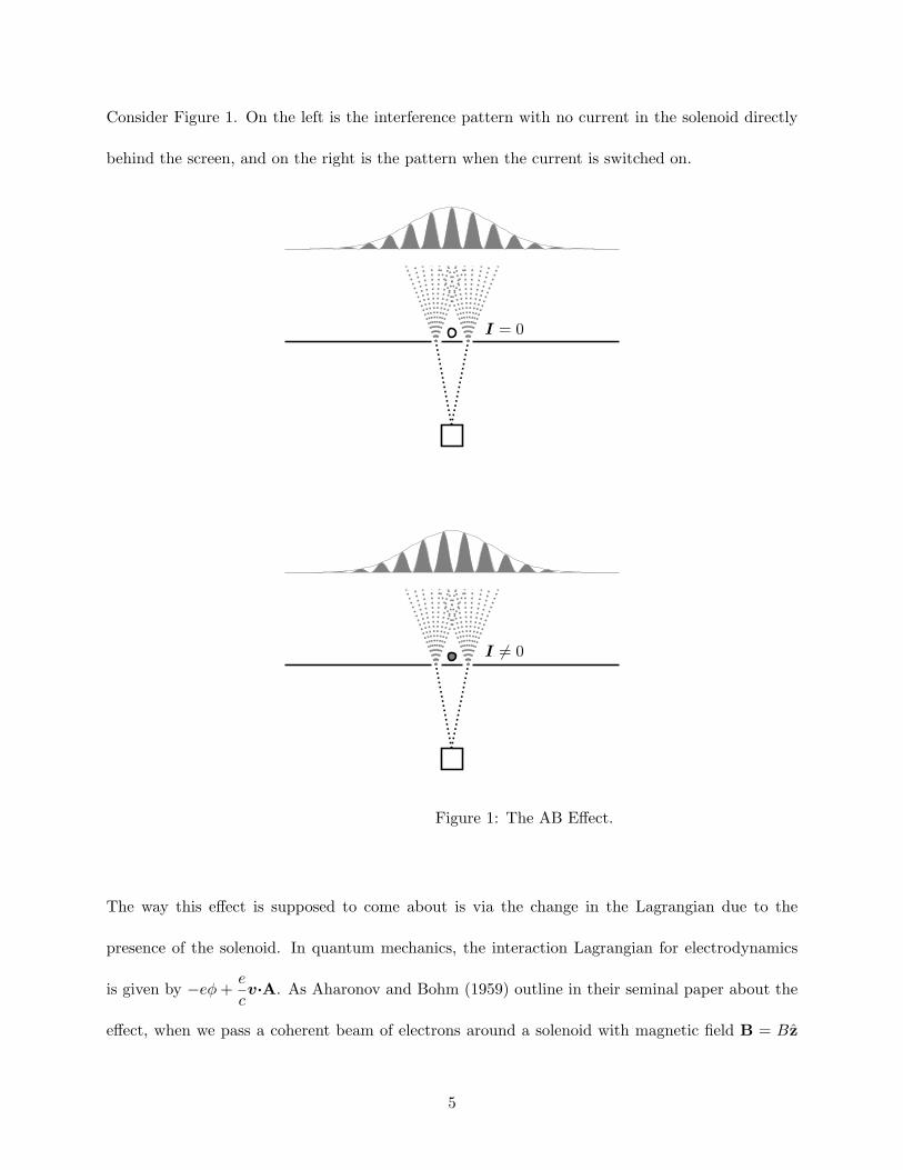
Consider Figure 1. On the left is the interference pattern with no current in the solenoid directly

behind the screen, and on the right is the pattern when the current is switched on.

I = 0

I 6= 0

Figure 1: The AB Effect.

The way this effect is supposed to come about is via the change in the Lagrangian due to the

presence of the solenoid. In quantum mechanics, the interaction Lagrangian for electrodynamics

is given by −eφ+e

cv·A. As Aharonov and Bohm (1959) outline in their seminal paper about the

effect, when we pass a coherent beam of electrons around a solenoid with magnetic field B = Bz

5

and vector-potential A =1ρBφ, we may consider the wave-function as split into two parts: ψ1

and ψ2. The phase of each beam will change along its path by a factore

c

xf∫xi

A · dx and thus

when the beams are brought back together the peaks of the interference pattern will have changed

from the situation when there is no current flowing in the solenoid. According to Aharonov and

Bohm, their thought experiment (now confirmed many times) shows that in quantum versions of

electrodynamics “we are led to regard Aµ(x) as a physical variable.”(491) Such a conclusion is

especially striking because in the classical theory, the potentials are no more than calculational

devices. Aharonov and Bohm make two related claims: that the potentials are ineleminable in

the formulation of quantum mechanics; that their effect shows that the potentials are necessarily

physically efficacious.

In the time since their paper was written it has been shown quite clearly that both claims are false

as stated. See, e.g., DeWitt (1962), Belinfante (1962), Mattingly (2006). See as well Aharonov and

Bohm (1962) in which they concede the formal correctness of DeWitt’s and Belinfante’s construc-

tions. This much at least is plain: there are several different ways to formulate electrodynamics

without potentials and still derive the AB effect within the theory. Naturally then it cannot be

necessary to take the potentials to be physically efficacious. However, it has become dogma that

we must either accept the reality of potentials in quantum mechanics and the problems attendant

thereto or accept other even less palatable and/or even less intuitive conclusions (e.g., nonlocal

field effects, or non-supervenience of the properties of a region on facts about that region alone,

etc.). This latter dogma is somewhat more plausible than Aharonov and Bohm’s 1959 claim, and

one flavor of it is given in their 1962 paper. The fact remains that the vast majority of physi-

cists and philosophers now do take the potentials as physically efficacious and then attempt to

6

make clear what philosophical consequences flow from such an adoption. As far as I know I am

the only philosopher who has attempted to show that the above dichotomy between non-locality

and novel metaphysics is incomplete. In my (2006) I display a gauge independent “potential” (a

proper, well-defined vector field) that can account for the effect, and I show how adopting this

potential commits us to none of the thorny problems associated with other methods of rejecting

gauge dependent potentials. But apparently even that construction has certain metaphysical nov-

elties, principally that my field appears to carry information but neither momentum nor energy.

Whether that appearance is correct will be considered another time, but for now I will set aside

that interpretation and give what is, in any case, a much more straightforward option4.

The various interpretations that have been proposed to account for the AB effect are now well-

known. See, e.g., Belot (1998), Leeds (1999), Mattingly (2006), and Healey (1997), (1999), and

also see especially Healey (forthcoming) for an exhaustive breakdown of all the various options

and his reactions to them. I will not canvas those options here but will merely note that it is

uncontroversially the consensus view that our understanding of electrodynamics must now change

markedly—either by introducing some form of non-locality, or indeterminism, or by reifying the

potential. I reject that view and claim instead that the AB effect shows us that field interactions

play a different role in quantum theory than in classical. Of course that is well-known, but I argue

that a full understanding of the AB effect highlights one important way in which those interactions

conflict with our classical intuitions: quantum objects are affected not by the net field of the various

objects with which they interact, but by the individual fields of those objects. Distributivity, in

the sense outlined above fails for quantum interactions.4Even if my potential does bear information, that feature of the potential is present in all analyses of the effect

that do not make use of the field strengths alone. So we might think that even if some metaphysical novelty is presentit is minimal in some sense.

7

2 The electromagnetic field

In the long and fascinating early history of electrodynamics, from the observations of the peculiar

effects of rubbed amber among the pre-socratics and of the stone of Heraclea (or magnet) described

by Socrates in Plato’s Ion, to the parlor tricks of the 17th and 18th Centuries, to the two-fluid model

developed by Franklin, Faraday’s contributions stand out for their striking clarity and for their im-

pressive novelty and explanatory power. The field concept changed forever our understanding not

only of electrodynamics, but of basic physics itself. Faraday’s conception of substantial lines of

electric and magnetic flux made possible our present understanding of forces between separated

bodies mediated by locally acting fields. However, after Maxwell’s mathematization of the the-

ory, and his attempts to find mechanical models, and then Einstein’s demonstration that electric

and magnetic fields cannot be uniquely separated out of a more general “electromagnetic” field,

Faraday’s intuitions seem to have lost their hold on our imaginations.

I suggest that Faraday’s insights can be adapted to the case of semiclassical electrodynamics (and

possibly quantum electrodynamics) to give an intuitive picture of how to account for the AB effect

completely locally in terms of electromagnetic field strengths alone. Thinking about the lines of flux

encountered by the moving electron will make sense of the electromagnetic term in the Lagrangian.

Notice now one key factor of Faraday’s lines of flux: they do not vanish when in contact with each

other, but rather “squeeze in” together. Beyond the imagery, what is the point of this suggestion?

I claim that focusing on the individual components of the electromagnetic field—rather than the

net field—will show quite clearly how the solenoid can appear to act where it is not. I claim further

that an appeal to the components of the field will show that all that is involved in the AB effect

are electromagnetic fields, and the peculiar non-distributive nature of quantum mechanical time

8

evolution.

2.1 Piecewise field descriptions

The theory of electrodynamics is linear, and we can think about this in two ways. First it is linear

in its solutions: for φ1 and φ2 possible solutions to the field equations, a1φ1 + a2φ2 is also possible

a solution for a1, a2 ∈ R. The values of a1, a2 are determined by boundary conditions.

Likewise the theory is linear in its solutions with respect to sources. That is, if the field of source S1

is φ1 and that of S2 is φ2 then the field of the combined sources S1, S2 is φ1 +φ2. For example, the

electric field of a point charge q at a distance r from the charge is Eq(r) = −∇φq(r) = −∇q

r=

q

r2r;

for two charges q1, q2 the field at the origin with q1 at r1 and q2 at r2 is Eq1,q2(r) = −∇φq1,q2(r) =

−∇[q1r1

+q2r2

]=q1r21

r1 +q2r22

r2 = Eq1 + Eq2 .

I will take advantage of this second sense of linearity in what follows to characterize the change in

the electron’s phase as arising from field strengths alone. The solenoid itself is a spiral of current

wrapped so tightly that it is essentially a stack of current loops. Likewise, these current loops are

themselves arrays of moving charges confined to the loops. Thus, we build the full solenoid out of

very many moving charges. Here’s how.

2.1.1 The field of a single element of current.

For what follows see, e.g., (Jackson, 1975, ch 14). The Lienard-Wiechert potential at space-

time point x of a single moving charge q moving with 4-velocity vµ at x′ is given by: Aµ(x) =

4πc

∫d4x′Dr(x− x′)Jµ(x′). Jµ(x) = qc

∫dτvµ(τ)δ(4)[x− r(τ)] is the effective current of the charge.

9

Dr(x− x′) =12πθ(x0 − x′

0)δ[(x− x′)2] is the retarded Green’s function restricting the influence of

the charge to the past light-cone of the observation point. The resulting expression for the magnetic

field B, in a frame where the velocity of the charge is v, divides into a part that goes like1R2

and

a part that goes like1R

(the radiative term):

B(x) = q

[β×n

γ2(1− β · n)3R2

]ret

+q

c

[n × (n− β) × β

(1− β · n)3R

]ret

(1)

Here R is the spatial distance from the observation point to the location of the charge when it

intersects the past light-cone of x, β =v

c, γ =

1√1− v2

c2

, β =dβ

dt, and n is a unit vector in that

(spatial) direction.

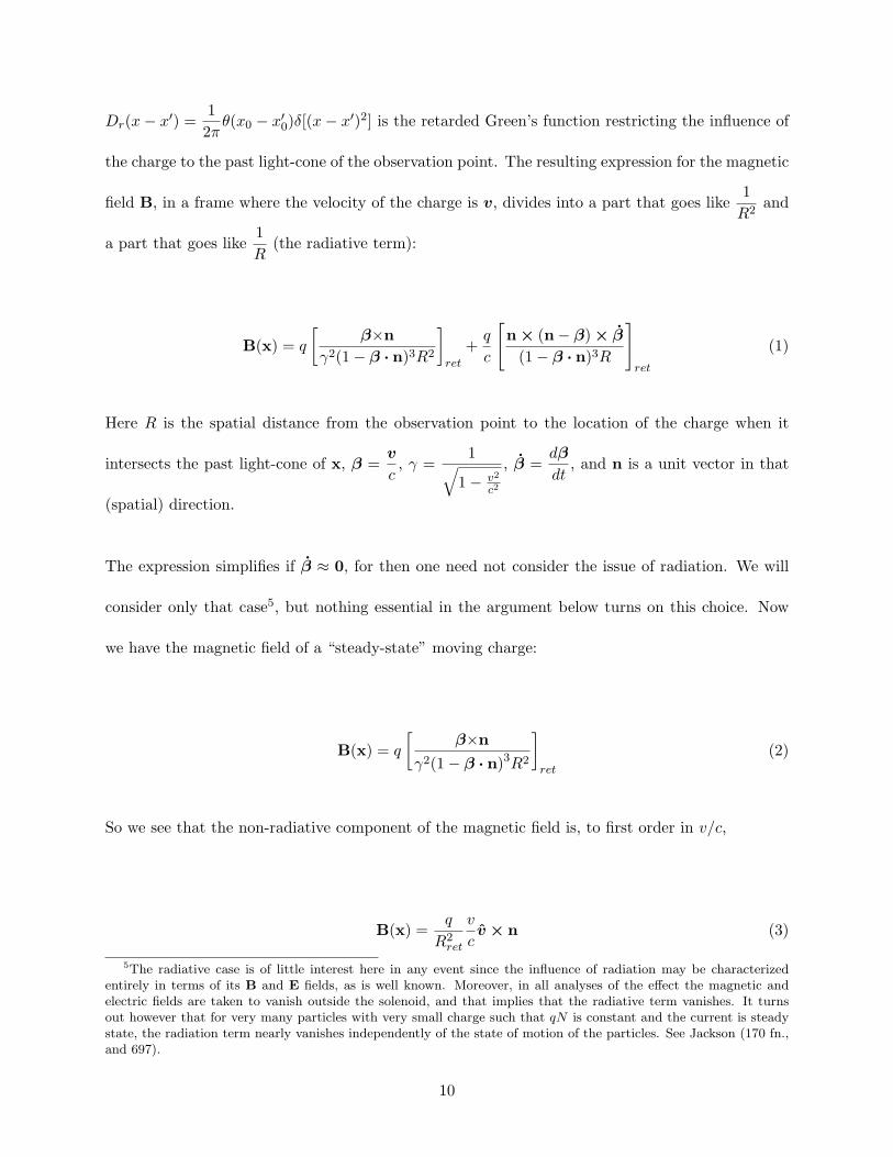
The expression simplifies if β ≈ 0, for then one need not consider the issue of radiation. We will

consider only that case5, but nothing essential in the argument below turns on this choice. Now

we have the magnetic field of a “steady-state” moving charge:

B(x) = q

[β×n

γ2(1− β · n)3R2

]ret

(2)

So we see that the non-radiative component of the magnetic field is, to first order in v/c,

B(x) =q

R2ret

v

cv × n (3)

5The radiative case is of little interest here in any event since the influence of radiation may be characterizedentirely in terms of its B and E fields, as is well known. Moreover, in all analyses of the effect the magnetic andelectric fields are taken to vanish outside the solenoid, and that implies that the radiative term vanishes. It turnsout however that for very many particles with very small charge such that qN is constant and the current is steadystate, the radiation term nearly vanishes independently of the state of motion of the particles. See Jackson (170 fn.,and 697).

10

and we recover the familiar1R2

dependence modified by a factorv

c.

2.2 The field of a single loop of current.

For further illustration we now confine the charge to a conducting loop and consider the magnetic

field that results from adding more individual charges. For slow-moving charges in a relatively

large loop, the acceleration of the individual charges is negligible, and we can continue to ignore

the radiative component of the field. For an observation point in the plane of the loop, the direction

of the field is either down into or up out of the plane of the loop, for the perpendicular component

of the motion of the charge to the right or left of the observation point respectively. Now, because

of the linearity of the theory, we can simply sum the first term on the right-hand side of Equation

2 over each of the charges in the loop:

B(x) =n∑i=1

qi

[β×n

γ2(1− β · n)3R2

]ret

(4)

2.3 The field of an infinite solenoid.

We could now continue and take a vertical array of current loops, tightly stacked, and extending

upward and downward effectively infinitely, i.e., an infinite solenoid. We will not carry out this

construction explicitly. First it would generate little insight because the mathematical burden is

so great, and would be carried out in terms of complete sets of orthogonal functions rather than

by way of elementary integrations over the field of the current loops themselves. This is because

the field of each loop outside the plane of that loop is extraordinarily complicated. Second, the

11

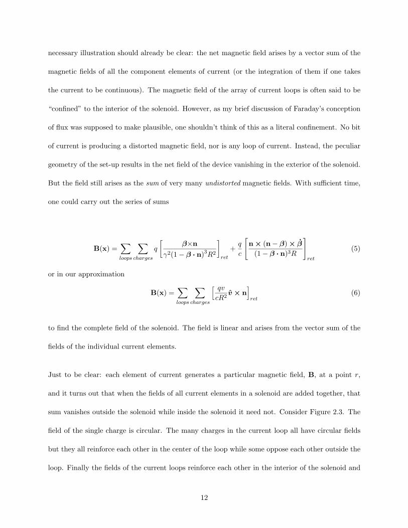
necessary illustration should already be clear: the net magnetic field arises by a vector sum of the

magnetic fields of all the component elements of current (or the integration of them if one takes

the current to be continuous). The magnetic field of the array of current loops is often said to be

“confined” to the interior of the solenoid. However, as my brief discussion of Faraday’s conception

of flux was supposed to make plausible, one shouldn’t think of this as a literal confinement. No bit

of current is producing a distorted magnetic field, nor is any loop of current. Instead, the peculiar

geometry of the set-up results in the net field of the device vanishing in the exterior of the solenoid.

But the field still arises as the sum of very many undistorted magnetic fields. With sufficient time,

one could carry out the series of sums

B(x) =∑loops

∑charges

q

[β×n

γ2(1− β · n)3R2

]ret

+q

c

[n × (n− β) × β

(1− β · n)3R

]ret

(5)

or in our approximation

B(x) =∑loops

∑charges

[ qv

cR2v × n

]ret

(6)

to find the complete field of the solenoid. The field is linear and arises from the vector sum of the

fields of the individual current elements.

Just to be clear: each element of current generates a particular magnetic field, B, at a point r,

and it turns out that when the fields of all current elements in a solenoid are added together, that

sum vanishes outside the solenoid while inside the solenoid it need not. Consider Figure 2.3. The

field of the single charge is circular. The many charges in the current loop all have circular fields

but they all reinforce each other in the center of the loop while some oppose each other outside the

loop. Finally the fields of the current loops reinforce each other in the interior of the solenoid and

12

oppose each other in its exterior.

B 6= 0

qa

qb

p1

p2Figure 2.1: Field of a (practically) infinite solenoid.

B(p1) =q

c

[v

(Rap1)2nap1×v +

v

(Rbp1)2nbp1×v + etc.

]ret

= 0

B(p2) =q

c

[v

(Rap2)2nap2×v +

v

(Rbp2)2nbp2×v + etc.

]ret

6= 0

Figure 2.2: Field of a current loop.

B(R) =n∑i=1

qi

[n × β

γ2(1− β · n)3(Rqi −R)2

]ret

Figure 2.3: Field of a current element.

B(R) =[ q

R2

v

cn × v

]ret

Now that we have been reminded of how the magnetic field comes about from the action of individual

charges, we can easily see how to understand the phase shift of electrons moving in the neighborhood

of a solenoid as arising directly from the magnetic fields of the current elements in the solenoid. It

13

will, I hope, become obvious that one can tell a story that involves nothing more than field strengths

and the motions of individual current elements. Neither novel fields nor indefinite potentials are

required.

I now move on to the main part of the construction. We will see how the action of the magnetic

fields of these current elements on the electron in the AB effect suffices to generate the phase shifts

responsible for the effect.

3 The AB Effect from magnetic fields alone

In outline, the construction is as follows: calculate the phase change of the electron due to the field

of a single element of current; sum over the current elements in a single loop; sum over loops in the

solenoid. We will see that calculating the phase change due to each element of current before we

sum over current elements can reproduce the total phase change required for the AB effect.

The force on a charge, q, moving in a magnetic field isq

cv × B. But what is the potential energy

associated with this force? Normally, for forces that are derivable from a potential, the difference

in potential energy between two points is simply the integral from one point to the other of F·dx.

But magnetic forces are funny in that they do no work (since the force is always perpendicular

to the velocity), and so for the actual travel of the particle, F·dx = F·dvdt = 0. So in the case

of magnetic interactions there is a question of what choice to make for the magnetic term that is

analogous to the electrostatic potential energy term. Jackson (1975) offers the following (I think

fairly typical) rationale: Since the interaction Lagrangian must be invariant under translations and

Lorentz transformations, the coordinates cannot appear explicitly. And this then constrains the

14

Lagrangian to the form (Jackson, 1975, p574):

Lint = − e

γcvαA

α or Lint = −eφ+e

cv · A (7)

The following considerations may give some further physical insight into this choice. Given the

parity between electric and magnetic fields that is made clear in the theory of relativity, presumably

there should be some parity of reasoning in how we arrive at the potential energy associated with

the two types of field. It cannot be, for example, that a shift to a frame where there is no magnetic

field changes the work required to produce a given configuration. And yet there seems to be little

discussion in the literature of how terms in v · A come to be associated with the potential energy

term in the Lagrangian. The geometry of spacetime itself helps us to understand the requirement

that the Lagrangian be covariant. But it does not give physical insight into the interactions recorded

by that Lagrangian. What we do know is that something is doing the work to bring about and

maintain the configuration of the system. So how should we think about this?

Here is Faraday’s intuitive picture of the energy state between two moving charges. Between the

charges, if they’re moving co-linearly, is an array of oppositely directed lines of flux (the circular

magnetic field created by moving charges), but these lines of flux are in the same direction for

points to the outside of both charges. By coming closer together, the width of the array, and hence

the total number of oppositely directed flux lines, is reduced. Similarly, for anti-co-linearly moving

charges, the widening of the array decreases the number of oppositely directed flux lines—but here

it is the opposing flux lines on the exterior of the array between the charges that decrease. As

Faraday observed, magnets distribute themselves so as to increase the co-linear and decrease the

15

anti-co-linear lines of flux between them. Packing anti-co-linear lines of flux together requires that

work be done on the field. One needn’t adopt this interpretation of course, but doing so can, I

hope, offer some insight into the nature of the potential energy as well as into how the magnetic

field is causing the fringe shift in the AB effect. The idea is that since these flux lines do not vanish

in the presence of other flux lines, they will still be acting on the electron. Although one needs to

generalize from magnetic and electric fields to electromagnetic, one can still suppose that lines of

flux (4-lines of flux) are indestructible, and interact directly with charges at their locations.

Another intuitive picture by which one might motivate the view that the flux from individual

charges can affect other charges comes this time from quantum field theory in its standard model

of particle physics. One common explanation for the interaction of charges on the standard model is

that the particles exchange the so-called force carriers—the gauge particles—of the theory. Without

going too deeply into this, and with all due caveats about the proper interpretation of Feynman

diagrams, and about the well-known interpretive problems of trying to give a particle ontology

for quantum field theory, and even about the fact that the way in which we standardly calculate

these forces is by passing to the potential formalism, one can see at least this: the action of these

particles, in exchanging force carriers, takes place independently of the action of other particles in

the system (assuming that the particles are not entangled). We treat the exchange between charges

individually even for very complicated field configurations. Looked at this way, the action of the

field on a moving charge is really the individual action of the many other charges in its vicinity.

Exchange of a virtual photon (in the electrodynamical case) is the field action between just two

charges, and it changes their phases accordingly.

Given these two intuitive stories then, we can see the potential as arising from the individual actions

16

of the various components of the current, even in the case of no net external magnetic field. Again

though, the facts of the matter seem to be independent of the persuasiveness or lack thereof that

one finds in these stories. We can, whatever story one likes to tell, sum the individual terms arising

from the individual current elements and even though the particle experiences no net force it still

responds to the presence of the component charges of the current through its change in phase; the

phase change itself arises from the time spent in the field, time spent with a given potential energy.

Clearly we can do the same trick with the dual AB effect. There, again, there is no net force but

we can see the potential energy as arising from a peculiar arrangement of charges, and the work

required to produce that arrangement. Were we to consider the interaction between each charge

in the Faraday cages and the electron wave components within those cages, we would find that

the integration of the forces over the distance separating the various charges sums to U , the total

potential energy.

We have now what I think is a clear proposal for how to eliminate all reference to potentials, and

moreover a clear proposal for how to account for the phenomena in terms of well-established physical

quantities—the magnetic and electric fields (electromagnetic field). We take the electromagnetic

potential energy terms in the Lagrangian to express the electromagnetic field energy necessary to

produce the field configuration, not the net field but rather the individual components of the field.

Whatever one thinks of the intuition pumps above, it should be obvious that we can carry out our

analysis in terms of electromagnetic fields alone—for the standard potential of a single charge is

non-zero just in case its electromagnetic field is non-zero, and the potential energy is a Lorentz

scalar in E and B.

Let me pause here to make two clarifying points. First it may appear to be obvious that there is

17

interaction between the solenoid and the external electron. For suppose that the net field inside the

solenoid is constant, then there must be work done to keep it constant as the magnetic field of the

electron increases at the location of the solenoid. Then suppose that the interior field is not constant,

in that case the current will have to overcome an increasing back-reaction force. Suggestions of

this sort that appeal to the possibility that the electron’s magnetic field penetrates the solenoid are

considered from time to time; see Boyer (2006) and references therein. Boyer also is challenging

the orthodoxy that the AB effect cannot arise from local field interactions, but from a perspective

significantly different from mine. If fact Boyer is attempting to account for the effect in terms of the

scattering of the electron’s magnetic field off the fields in the interior of the solenoid. There seems to

be a consensus that Peshkin’s critique of such programs is decisive (Peshkin and Tonomura, 1989).

(Thanks to an anonymous referee for prompting me to highlight Peshkin’s account.) However my

proposal here is independent of the above issue, for I consider only the component magnetic fields

exterior to the solenoid. However a related worry does arise concerning the possibility of magnetic

fields exterior to the solenoid. In the most definitive tests of the effect by Tonomura et al. (Peshkin

and Tonomura, 1989) the solenoid is enclosed in a superconducting shield. In that case the Meissner

effect would prevent all magnetic fields from penetrating the superconductor and so there would

be no magnetic fields at all in the path of the electron. (An anonymous referee has made this

suggestion as did Yakir Aharonov in conversation.) But that is simply to assume the point at issue:

whether there are component fields acting in a region in which the net fields vanish identically.

The Meissner effect appears to be perfectly consistent with the vanishing of net but not component

fields. For what but a redistribution of currents, and hence the fields that they produce, enforces

the vanishing of the net field in the interior of the superconductor? Absent further argument, and

I am not aware of any explicit treatment of this in the literature, there is simply no reason to think

18

that the physics of superconductivity is at odds with the proposal that component fields are active

in the exterior of the superconducting shield. If my proposal is correct then only a test along the

lines of the AB effect would reveal the action of these component fields, and on my proposal that

is just what the AB effect does reveal.

3.1 The AB Lagrangian

To show explicitly that it is possible to account for the AB effect in terms of the interaction between

the individual charges, I now display that account for the simple case we have been considering. In

our approximation of slowly changing and hence non-radiating fields, the appropriate Lagrangian

is properly expressed in the Darwin form, which is correct to second order inv

c. This form is also

instructive because it expresses the potential energy explicitly in terms of the interactions between

the charges.

The Darwin Lagrangian for a charge, a, in the field produced by a collection of charges, for fixed

motion of the other charges is:

La =mav

2a

2+

18mav

4a

c2− ea

∑b6=a

ebRab

+ea2c2

∑b6=a

ebRab

[va · vb + (va · nab)(vb · nab)] (8)

Although messy, it is instructive to express the final term as an interaction between the moving

charge, a and the magnetic fields of the other charges. For a given charge b:

ebRab

vb = Bb|aRab c vb

sin(θRab,vb)

def= Bb|aκ (9)

19

Here Bb|a is the magnetic field of the charge b evaluated at the location of charge a. κ is a vector

characterizing b’s state of motion and location relative to a.

We may now express the Lagrangian as:

La =mav

2a

2+

18mav

4a

c2− ea

∑b6=a

ebRab

+ea2c2

∑b6=a

Bb|a κ · [va + nab(va · nab)] (10)

Now we examine the terms on the right hand side of the equation. The first term is the kinetic

energy of the moving charge to first order inv

c; the second term is the second order correction

to the kinetic energy. The third term is the Coulomb interaction between the moving charge and

each of the charges in the collection. Since the net charge vanishes, so too does this term in the

Lagrangian. The last term is the magnetic interaction energy between the moving charge and the

moving charges in the array.

In standard presentations of the AB effect (for example Quigg (1997) and indeed implicitly in

Aharonov and Bohm’s (1959)) it is recalled that if ψ0(t,x) is a given wave function of a free

particle with charge e in the absence of electromagnetic fields then in the presence of such fields:

ψ(t,x) = eiSemψ0(t,x) = ei

tR0

Lemdt′

ψ0(t,x) (11)

where Sem, Lem are the action and Lagrangian respectively that arise from the interaction of the

particle with the fields.6 We can then take the change in phase due to the electromagnetic interac-6For an illuminating discussion of the action principle for electromagnetism see Landau and Lifshitz (1975) §§16,

20

tion for a time, t, to bet∫0

Ldt′ and the infinitesimal phase change to be Ldt. And we can conclude

that for otherwise free particles travelling different paths under the influence of electromagnetic

fields that after a time t the change in phase due to that influence is:

∆φ = ∆φψ1 −∆φψ2 =

t∫0

(Lem1 − Lem2)dt (12)

A suitable choice for the Lagrangian, and the one we normally choose is

Lem =e

cA·dv − eφ (13)

On the other hand, one is also free in this limit to make the choice of the Darwin Lagrangian.

Therefore we can simply take

ψ(t,x) = ei

tR0

−eaP

b6=aeb

Rab+ ea

2c2

Pb6=a Bb|a κ·[va+nab(va·nab)]dt

′

ψ0(t,x)

= ei

tR0

ea2c2

Pb6=a Bb|a κ·[va+nab(va·nab)]dt

′

ψ0(t,x)

(14)

for the situation described above.

If we now assume, arguendo, that the phase of each of the components of the electron wave function

is determinate at each instant7 we can see that the instantaneous change in the phase difference

26, and 27.7This is not strictly speaking necessary, though I think it is correct. We need only assume only that the instanta-

21

between the components is (Lψ1 − Lψ2)dt. But note that Lψ1 and Lψ2 are, as we have shown,

expressible in terms of the individual magnetic fields of the current elements. Thus it is possible to

write the infinitesimal relative change in phase as a function of the magnetic interaction between

the travelling electron and the charges in the solenoid. Then integrating over the time of travel will

give the total phase difference between the components in agreement with the standard prediction

for the AB effect. That is:

∆φ = ∆φψ1 −∆φψ2 =

t∫0

(Lem1 − Lem2)dt

=

t∫0

e

2c2

∑b6=e1

Bb κ · [ve1 + nbe1(ve1·nbe1)]−∑b6=e2

Bb κ · [ve2 + nbe2(ve2·nbe2)]

dt′=e

c

t∫0

(A1 · v1 −A2 · v2)dt′ =e

c

x∫0

(A1 · dx1 −A2·dx2) =e

c

∮A·dx

(15)

And this equation holds for any A whatever, since all differences between potentials vanish under

loop integration.

Note that we have not “fixed a gauge” here. Gauge fixing is a mathematical operation that

one carries out in choosing a particular vector potential consistent with Maxwell’s equations and

satisfying some desiderata or other. We have not done that. Instead we have written down an

expression characterizing the effect on the wave function that arises from what I am arguing are

the actual magnetic fields that are present at the location of the electron. It is an interesting fact,

neous change in the relative phase between the beam components that is in fact due to the electromagnetic fields isitself determinate—that suffices to account for the effect itself in terms of the magnetic fields alone. The question ofhow to think about the phase remains. See Section 4 for a speculative and necessarily brief discussion of this point.

22

worth some analysis, that one can translate this expression into one involving a particular choice of

vector potential. But that fact is irrelevant to the present analysis. We have assumed at the outset

some determinate wave function when the beam first divides, and we observe the change in phase

due to the magnetic field that results from travel along the different paths. Of course one may

choose to add terms to the Lagrangian of the form ∇λ or one may instead choose to add terms

to the electron phase—and then these choices will have to be made mutually consistent. But one

virtue of the preceding account is to make clear that such terms are merely additions allowed by

the formalism that have nothing to do with the interactions between the charges.

Because of the way the terms in the Darwin Lagrangian arise they appear to correspond to terms

in the non-relativistic Lienard-Wiechert potentials, which can be arrived at by imposing a Lorentz

gauge condition. So one may well still wonder how this discussion does connect to various proposals

for “fixing a gauge”. The best way to look at the issue is, I think, to stop thinking of gauge as con-

nected to electrodynamics itself and to think of it as part of our choice of representational strategy.

There is an important mathematical relationship between how we represent the Lagrangian and

how we represent the electron phase. There is, however, no obvious reason why one should connect

that relationship directly to electrodynamics. Further discussion of this point is beyond my scope

here.8

The AB effect, and all of electrodynamics essentially, is encoded in the electromagnetic field

strengths (together with the charge-current diistribution); for understanding the actual physics,

the potentials are an irrelevant artifact. The vector potential remains merely a powerful calcu-

lational device—as it was in the classical theory. At the same time note that the AB effect is a8I am very grateful to an anonymous referee both for urging me to make the above discussion more explicit and to

clarify the role of the Darwin Lagrangian in the application of the action principle, and also for helpful suggestionsabout how to do so.

23

terrible device for measuring the actual current since it is sensitive only to the value of the holon-

omy and that under-determines the value of the current. It would seem an illegitimate return to

verificationist scruples to assume that the only physics is the physics that is revealed directly by

that effect.

We have now seen the AB effect accounted for entirely in terms of locally operative, deterministic,

electrodynamical field strengths. I think the conclusion is obvious. We should not take seriously

such quantities as the net field. When we do take these quantities seriously, and think that only the

net field can act we are led naturally to think that in certain circumstances new fields are required.

The fact that there is no net field however has very little to say about what processes are actually

taking place. The construction laid out here shows clearly that there is a function, f , such that∑i f(Bi) = ∆φ; whereas there is no g such that g(

∑iBi) = ∆φ. The sum of the effects cannot

be rewritten as the effect of a sum. Because the peculiar geometry of the solenoid leads to the

vanishing of the net magnetic field (and hence our normal measure of the field, the Lorentz force)

we are tempted to think that there are no locally present magnetic fields. While the vanishing of

the net field obscures the role of the magnetic field in changing the electron phase, the AB effect

should remind us of just this fact: the phase of the wave function is affected not by net fields but

by the individual field components.

3.2 Other gauge theories

Before I conclude this section, I raise the question of how this story is to connect with our accounts

of other gauge theories. First, the electromagnetic account—compelling physical story or no—

certainly establishes my main claim: Gauge theories do not, in general, entail any fancy new

24

metaphysics. But second I speculate that an exclusive focus on the mathematical form of the

constraints arising in our physics is a mistake and that a more fruitful approach would involve

explicitly addressing the origin of these constraints. We can learn much from the methods of

gauge-theoretic analysis, but what we cannot learn directly through these methods is what the

underlying fields are. When we focus on the gauge field itself as causally relevant we close off any

route to an intrinsic causal account in terms of the underlying physical fields. The equations of

motion follow from the constraints acting on the system, and the Lagrangian itself—but insight into

the causally relevant formulation of the Lagrangian, and hence the causally relevant field does not

follow. We have seen over the last several decades the fruitfulness of trying to extract deep insight

into quantum electrodynamics from a consideration alone of its character as a gauge theory. Perhaps

now it is time to turn our attention back to the underlying physical system itself—the currents

and their electromagnetic fields. The general question of how to understand the application of

Lagrangian methods to physical systems, though of crucial importance, is beyond the scope of this

work.

4 Interlude on the quantum phase

A standard view of the role of the quantum phase is endemic in the literature, and a difficulty with

this view for understanding the way physical systems are best to be represented in their interactions

is clearly apparent in treatments of the AB effect. What follows is an attempt to overcome my own

difficulty in coming fully to understand the quantum phase and is therefore quite tentative. All I

have to offer is an analogy that may help make clear how I think the phase is best understood.

Consider the case of velocity. There is a sense in which relativity (Galilean and Einsteinian) has

25

shown us that velocity is irreal. We are free, at each point on the trajectory of a particle, to choose

the inertial frame in which we will describe the motion of that particle, and we are therefore free

to assign to it any velocity we choose (but less than c, of course, in STR). In analogy with the

phase case, I can adopt infinitesimal local inertial frames and knit them together in just the right

way so that there are no observable consequences of my local choices. Doesn’t this freedom then

demonstrates that velocity is unreal? Not necessarily. Such freedom shows only that velocity is

relative to a choice of inertial frame and, moreover, once I specify an inertial frame, no-one suggests

that those forces in my frame of description that change the velocity of the particle in that frame

are not really changing the velocity of the particle. It may be possible to make a time-dependent

choice of frame such that the particle is always described as moving at the same velocity under

that choice. But clearly the constancy of the particle’s velocity is an artifact of my choice of

representation scheme. The freedom I have to make this choice does not by itself suggest that there

is something unreal about velocity.

Similarly the fact that I have complete liberty to specify locally the phase of a quantum system—as

long as these local choices knit together properly where they overlap—should not suggest to me

that the phase itself is unreal. The numerical value of the phase is certainly highly non-trivially

influenced by my choices, but there is reason to think that there is a fact about the phase itself and

the way it is being affected physically that is independent of these representational schemes. Two

electron wave functions that arise from splitting a single wave function into two components have

phases that are real, and that are similarly affected by the magnetic fields of the elements of the

current in the solenoid. And as the time parameter increases, the phases have real significance for

the behavior of the total system. So while the actual value of the phase at any point on the electron’s

path is not independent of my choice of phase assignment, the difference between the phase that

26

arises from travelling distinct paths is determinate and independent of my phase convention.

That the phase of the electron components in the AB effect are only specified relative to each

other no more suggests that their phases are unreal than does the relativity of velocity suggest

that velocity itself is unreal. It is then, I maintain, perfectly appropriate to treat the change in

phase along the electron path as determinate at each point on that path. This treatment involves

reifying the phase, but not making distinct wave functions out of wave functions differing only in

phase value (as Leeds (1999) for example fears). Nothing in my account should suggest that I take

the value of the phase to be fixed by the theory. One is still free to assign a phase transformation,

but one needn’t think of that as having anything to do with electrodynamics itself. Rather such a

transformation requires its own complementary, compensatory term in the Lagrangian.

5 Conclusion

One might not be persuaded by the physical explanation of the Lagrangian term above. Indeed, an

obvious objection to the above story is the following: Why should we think of the magnetic field

as changing the phase, and more generally, why should the Lagrangian be modified by that factor

rather than by the potential term as is more traditional? Even granting that we can calculate the

lines of flux as claimed, why should those be part of our causal story?

To this objection there is little to respond that is truly decisive. But the following considerations are

relevant, and I think powerful. First, why should the vector potential itself modify the Lagrangian?

Is it only because it arises in the mathematical form that it does—as that quantity vector calculus

tells us must arise whenever there is a divergenceless field in the neighborhood, or a quantity that

27

has the right transformation properties? But if that is our only motivation for using the potential

term, then it has no conceptual advantage over the more familiar electromagnetic field. If that is

right, then having a conceptual story about the action of the fields of the individual elements of

current should be an advantage. That advantage is enhanced when we note that the story in terms

of magnetic field components is completely well-defined, gauge independent, and local. (And for

those for whom such is itself an advantage, the account is ontologically parsimonious.)

There is a kind of blend of prospective and retrospective physical legitimacy account to be given

here. We do, in fact, as the vast literature on the AB effect makes clear, consider the electromagnetic

field strengths to be better physical quantities than the potentials. All things being equal, a story

told in terms of electromagnetic fields should be more compelling than one that relies on the

unphysical potential terms. Given the mathematical form of the account above, the insight that

the density of flux experienced by the electron is at the root of its phase shift arises naturally.

I merely highlight now the following claim, but I will not here argue for it in detail. The story as

I have told it in terms of current elements is not restricted to any particular account of the micro-

physics. As long as the smallest portions of any bulk matter that gives rise to magnetic fields are

treated as themselves giving rise to sub-components of the net field, the technique above will work

as advertised. For the traditional potentials can themselves be generated from the infinitesimal

charge-current elements, and these infinitesimal components can be re-conceived as generating the

infinitesimal components of the flux field. And all of the standard story underlying the AB effect

does treat the bits of matter in bulk as required on such a view.

A serious question remains however. How is it that the fields arising from the individual elements

do not simply vanish? How can they continue to be causally active when their net field vanishes?

28

Here another analogy might help. When we illustrate the force composition law for mechanical

systems, it is sometimes useful to consider many strings attached to a single mass. As forces are

applied to these various strings and equilibrium is reached, we do not claim that there is no force

acting on the mass. Instead, we calculate the acceleration of the mass by finding the result due

to each individual string. The strings are still there, as are the components of the force. Even

more relevant is the case of a boat tied at dock. If the tensions in the various ropes are such that

their vector sum vanishes, then the boat will be stationary. But it would be madness to think that

no forces are acting on the boat. Clearly sufficient tension in the ropes will tear the boat apart.

(Similarly, as a colleague has quipped, the assurance that no net forces are present will be cold

comfort to a prisoner sentenced to be drawn and quartered—our victim is torn apart in any case.)

I claim that something relevantly analogous is happening in the case of electrodynamics; I claim

that the individual field elements are still present and that they interact individually with the

electron as though it were in the flux field whose action is as I have described above. Naturally the

electron is not torn apart, but its phase does change—and continues to change even when no net

force is acting.

Consider how one might react who is ignorant of the history of this debate: When told about

the Lagrangian for electromagnetism she might reply that the A term appearing there is simply a

mathematical convenience, but that what is really going on arises from the B field. Challenged,

she might follow just the line of argument outlined above and claim that something to do with the

magnetic flux density along the path of a charge is the relevant term to add to the Lagrangian.

One important lesson to be drawn from this discussion is that it is sensible to suppose that the net

field is fictional while the component field is factual. But how can this be? First note that there

29

is nothing the net field does that the components of the field together cannot do—if there is a net

force it is equal in strength to the vector sum of the component forces; the radiative propagation

of the net magnetic field is equal in magnitude to the sum of the radiation from the components

fields; etc. But here we have found something else that can be done by the component fields that

manifestly cannot be done by the net field.

So since we know that the individual bits of charge-current are still producing their own fields (how

else could a net field arise?) why should we hesitate to recognize the distinction between net and

component fields, and accord significance only to the latter? On the other hand in light of the

well-known worries over non-locality, etc., that arise out of standard accounts of the effect, it is

perhaps no longer sensible to suppose the contrary and to insist that, since the net field cannot

produce all of the relevant physical effects, there must be some novel entity that does. At any rate,

there is no particular pressure on us to adopt new metaphysics in the light of the Aharonov-Bohm

effect. Surely this is what Faraday would reply.

30

References

Aharonov, Y. and Bohm, D. (1959). Significance of electromagnetic potentials in the quantumtheory. Physical Review, 115 (3): 485-491

Aharonov, Y. and Bohm, D. (1962). Remarks on the possibility of quantum electrodynamicswithout potentials. Physical Review, 125 (6), 2192-2193.

Belinfante, F. (1962). Consequences of the postulate of a complete commuting set of observablesin quantum electrodynamics. Physical Review, 128 (6), 2832-2837.

Boyer, T. ( 2006). Darwin-Lagrangian analysis for the interaction of a point charge and a magnet:considerations related to the controversy regarding the AharonovBohm and AharonovCasher phaseshifts. Journal of Physics A, 39, 3455-3477.

Belot, G. (1998). Understanding electromagnetism. British Journal for Philosophy of Science, 49(4), 531-555.

Cao, T. (1999) (ed.). Conceptual foundations of quantum field theory (pp. 298-309). Cambridge:Cambridge University Press.

DeWitt, B. (1962). Quantum theory without electromagnetic potentials. Physical Review 125 (6),2189-2191.

Healey, R. (1997). Non-locality and the Aharonov-Bohm effect. Philosophy of Science, 64, 18-41.

Healey, R. (1999). Is the Aharonov-Bohm effect local? In Cao, T. (1999).

Healey, R. (In press). Gauging what’s real. Cambridge: Cambridge University Press.

Jackson, J. (1975). Classical electrodynamics. New York: John Wiley & Sons.

Landau, L. and Lifshitz, E. (1975). The classical theory of fields. New York, NY: Elsevier.

Leeds, S. (1999). Gauges, Aharonov, Bohm, Yang, Healey. Philosophy of Science (4), 66, 606-627.

Martin, C. (2002). Gauge principles, gauge arguments, and the logic of nature”, Philosophy ofScience, 69 (3), S221-S234.

Mattingly, J. (2006). Which gauge matters. Studies in History and Philosophy of Modern Physics,37, 243-262.

Peshkin, M. and Tonomura, A. (1989). The Aharonov-Bohm effect, lecture notes in physics 340.New York, NY: Springer-Verlag.

Quigg, C. (1997). Gauge theories of the strong, weak, and electromagnetic interactions. Reading,

31

MA: Addison-Wesley.

32