Classical Inflow Models

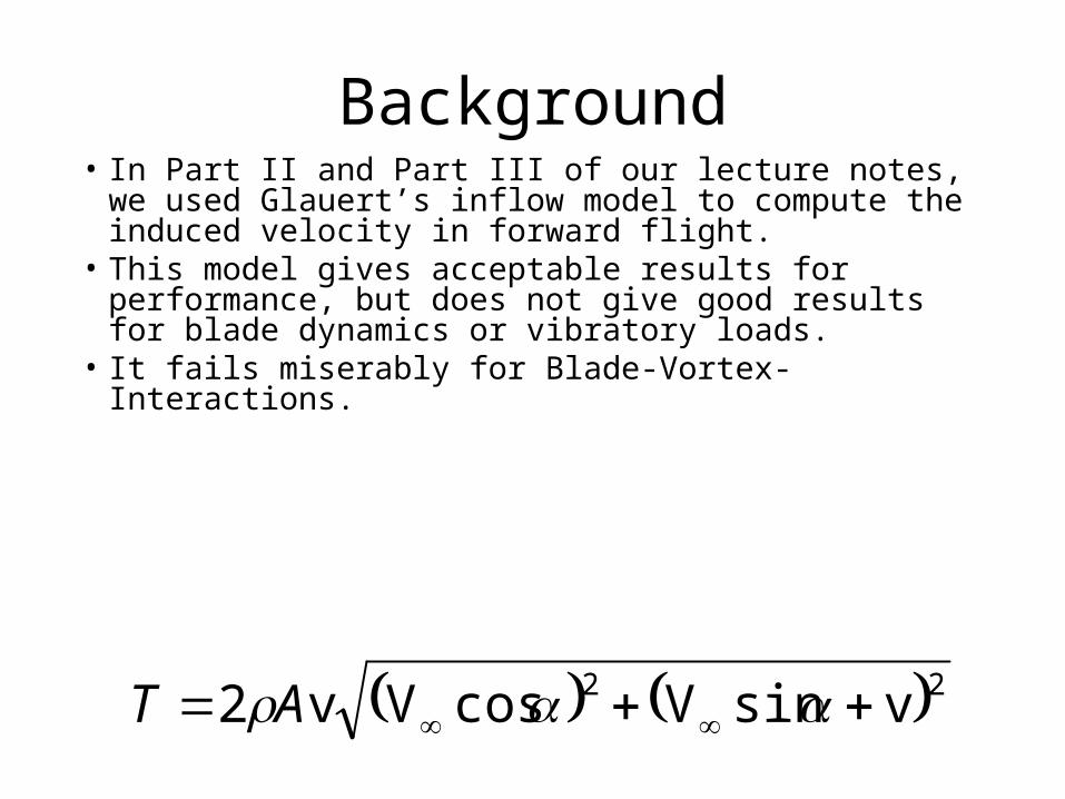
Background• In Part II and Part III of our lecture notes, we used

Glauert’s inflow model to compute the induced velocity in forward flight.

• This model gives acceptable results for performance, but does not give good results for blade dynamics or vibratory loads.

• It fails miserably for Blade-Vortex-Interactions.

22 vsinVcosVv2 AT

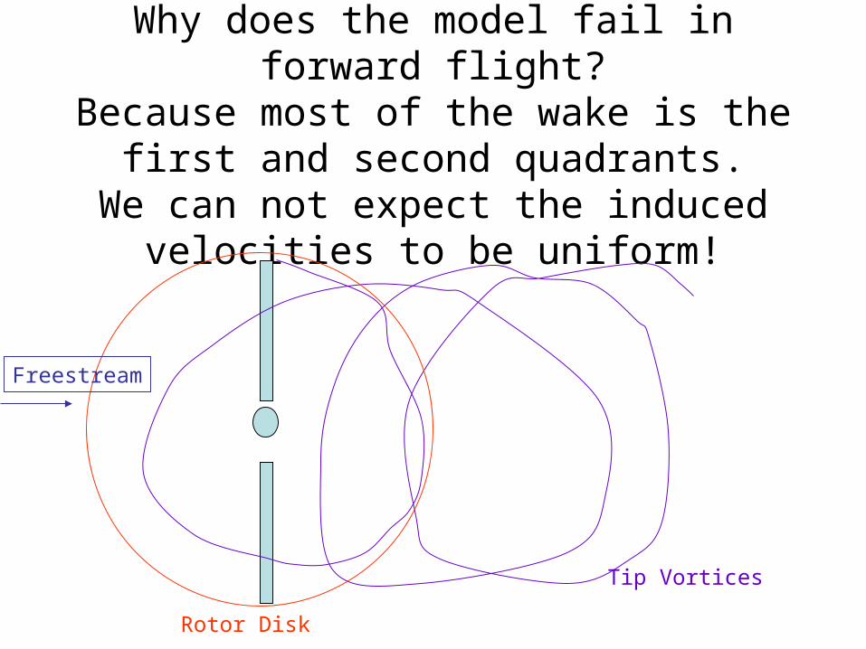
Why does the model fail in forward flight?Because most of the wake is the first and

second quadrants.We can not expect the induced velocities to

be uniform!

Rotor Disk

Tip Vortices

Freestream

Experiment by Harris

• Because most of the tip vortices are in the first and fourth quadrants, the induced velocity associated with these vorticies (i.e. the inflow) is very high in the first and fourth quadrants.

• The resultant reduced angle of attack leads to smaller lift forces in the aft region, compared to uniform inflow model.

• The blade responds to this reduced loads 90 degrees later.

• It flaps down (leading to a more negative 1s) more than expected.

• Harris experimentally observed this, in a paper published in 1972 in the Journal of the American Helicopter Society (See Wayne Johnson, page 274, figure 5-39).

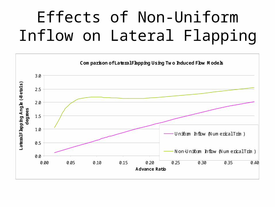
Effects of Non-Uniform Inflow on Lateral Flapping

Comparison of Lateral Flapping Using Two Induced Flow Models

0.0

0.5

1.0

1.5

2.0

2.5

3.0

0.00 0.05 0.10 0.15 0.20 0.25 0.30 0.35 0.40

Advance Ratio

Lat

eral

Fla

pp

ing

An

gle

(-B

eta1

s)

deg

rees

Uniform Inflow (Numerical Trim)

Non-Uniform Inflow (Numerical Trim)

Effects of Non-Uniform Inflow on Blade-Vortex-Interaction Loads

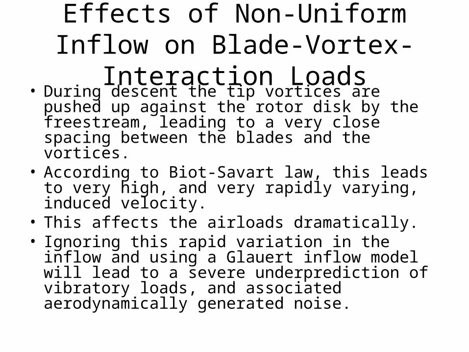
• During descent the tip vortices are pushed up against the rotor disk by the freestream, leading to a very close spacing between the blades and the vortices.

• According to Biot-Savart law, this leads to very high, and very rapidly varying, induced velocity.

• This affects the airloads dramatically.• Ignoring this rapid variation in the inflow and

using a Glauert inflow model will lead to a severe underprediction of vibratory loads, and associated aerodynamically generated noise.

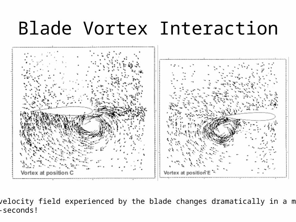
Blade Vortex Interaction

The velocity field experienced by the blade changes dramatically in a matter ofmili-seconds!

Efforts to Improve Inflow Models

• Engineers and researchers recognized very quickly that there is need for improvements in the inflow model.

• Until the mid 1960s, the work was analytical or semi-empirical. This approach is called classical vortex theory. See pages 134-141 of text, and our web site.

• Starting 1960s, numerical approaches based on Biot-Savart law became popular.

Coleman’s Model

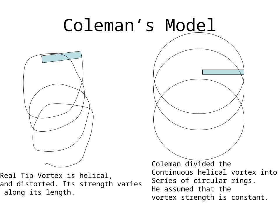
Real Tip Vortex is helical,and distorted. Its strength varies along its length.

Coleman divided theContinuous helical vortex into aSeries of circular rings.He assumed that the vortex strength is constant.

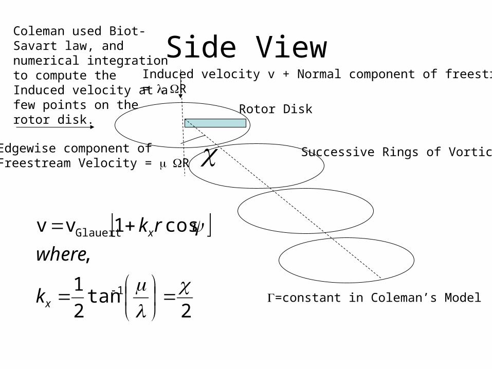
Side View

2tan

2

1

,

cos1vv

1

Glauert

x

x

k

where

rk

Rotor Disk

Successive Rings of VorticesEdgewise component ofFreestream Velocity = R

Induced velocity v + Normal component of freestream= R

=constant in Coleman’s Model

Coleman used Biot-Savart law, and numerical integration to compute theInduced velocity at a few points on the rotor disk.

Castles’ et al’s Model

• This model is discussed in NACA report 1184. A pdf file may be found at the web site: http://www.ae.gatech.edu/~lsankar/AE6070.Fall2002/castles.pdf

• Castles replaced the numerical integration in Coleman’s model with analytical integration.

• These authors also replaced the individual rings by a continuous sheet of vorticity.

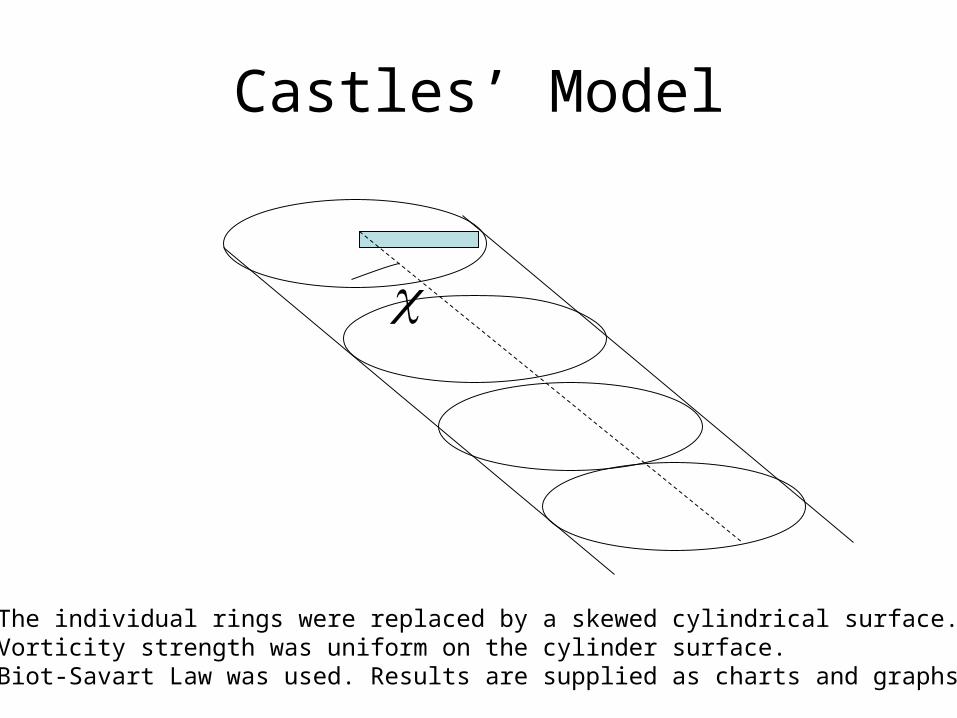
Castles’ Model

The individual rings were replaced by a skewed cylindrical surface.Vorticity strength was uniform on the cylinder surface.Biot-Savart Law was used. Results are supplied as charts and graphs.

Heyson et al’s Model

• This model is discussed in the NACA Report 1319. An electronic version may be found at: http://www.ae.gatech.edu/~lsankar/AE6070.Fall2002/heyson.pdf

• This model rectifies one of the assumptions in Castles’ and Coleman’s models, namely that the rotor only sheds tip vortices.

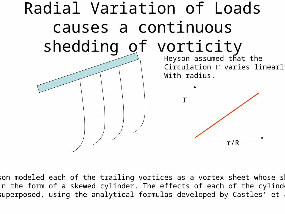
Radial Variation of Loads causes a continuous shedding of vorticity

Heyson assumed that theCirculation varies linearlyWith radius.

r/R

Heyson modeled each of the trailing vortices as a vortex sheet whose shapeis in the form of a skewed cylinder. The effects of each of the cylinders maybe superposed, using the analytical formulas developed by Castles’ et al.

Heyson’s Model

At each radial locationA vortex sheet of shapeSimilar to a circularCylinder is shed.

The strength is constant,Both along the axis of the Cylinder and around the azimuth.

Advanced Inflow Models

Background

• Around 1965, more powerful digital computers became readily available.

• Engineers began to model the tip vortex as a skewed, distorted, helix.

• The strength of the tip vortex was allowed to vary with azimuth, acknowledging the fact that the blade loading changes with the azimuthal position of the blade.

Background (Continued)

• Sadler at Bell Helicopter, and Scully at MIT developed some of the earliest techniques.

• Sadler used a rigid helical wake, while Scully allowed for the wake to deform due to self-induced velocities.

• The induced velocity at the “strips” on the blade were computed using Biot-Savart Law.

• Modern methods (e.g. CAMRAD-II) not only model the tip vortex, but also the inboard vortices, and shed vortices.

• See our web site for several publications related to CAMRAD-II.

Shed Wake

When the lift (or bound circulation) around an airfoil changes with time, Circulation that is equal in magnitude to the bound circulation but oppositeIn strength is shed into the wake.

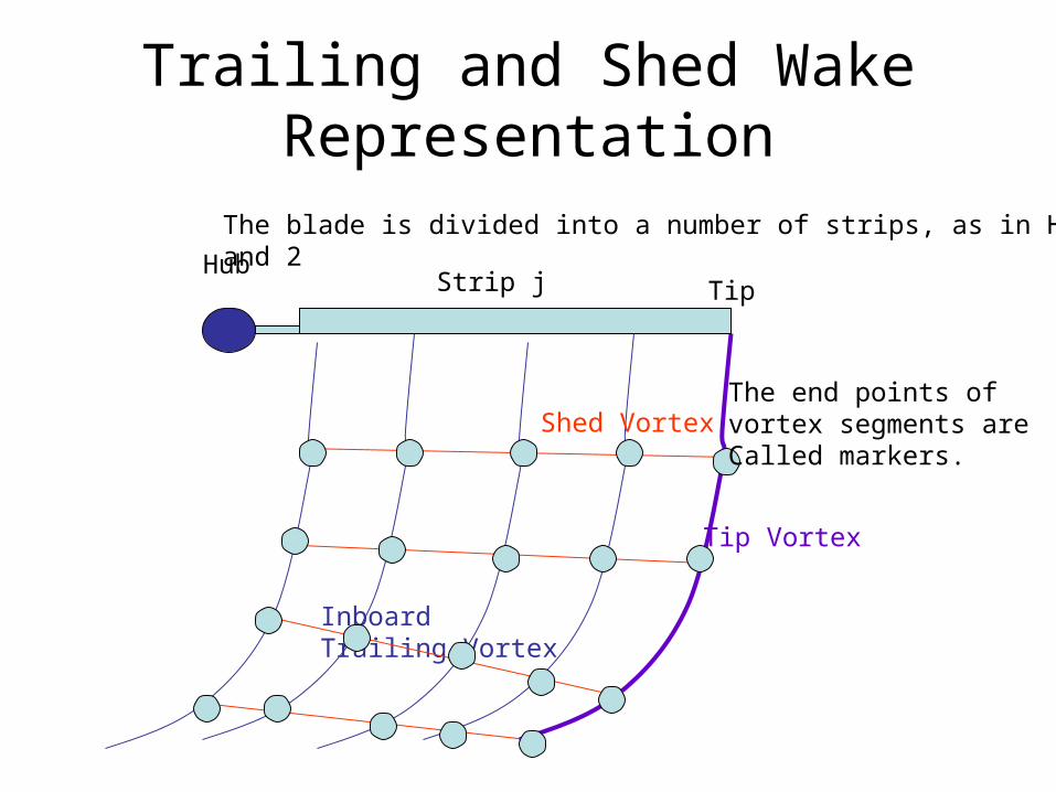
Trailing and Shed Wake Representation

Tip Vortex

InboardTrailing Vortex

Shed Vortex

HubTip

The blade is divided into a number of strips, as in HW#1 and 2

Strip j

The end points of vortex segments areCalled markers.

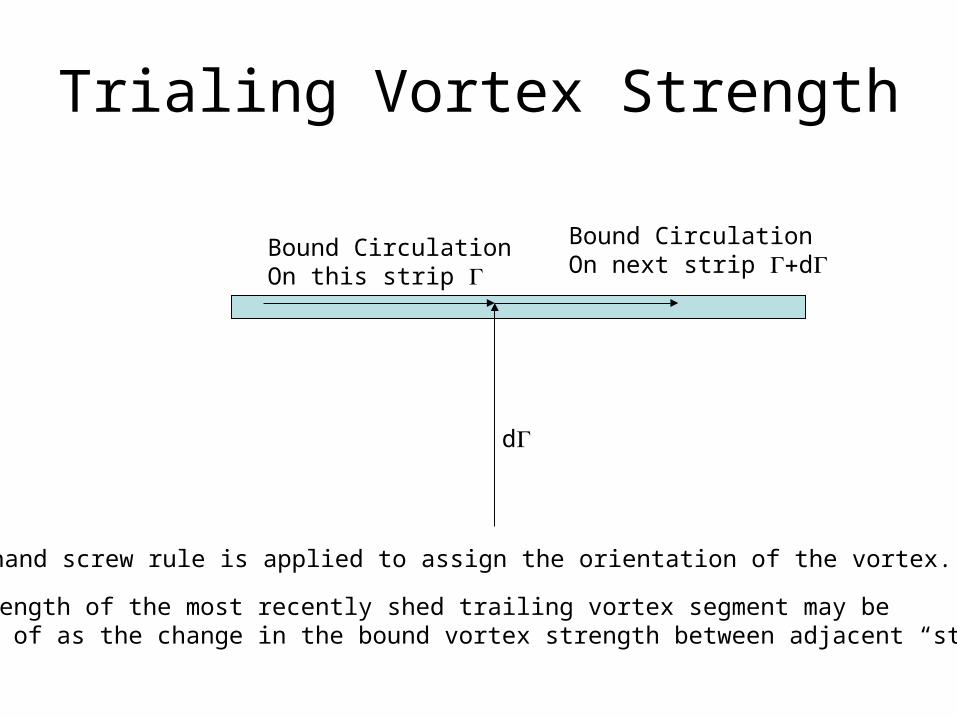
Trialing Vortex Strength

Bound CirculationOn this strip

Bound CirculationOn next strip d

d

The strength of the most recently shed trailing vortex segment may bethought of as the change in the bound vortex strength between adjacent “strips.”

Right hand screw rule is applied to assign the orientation of the vortex.

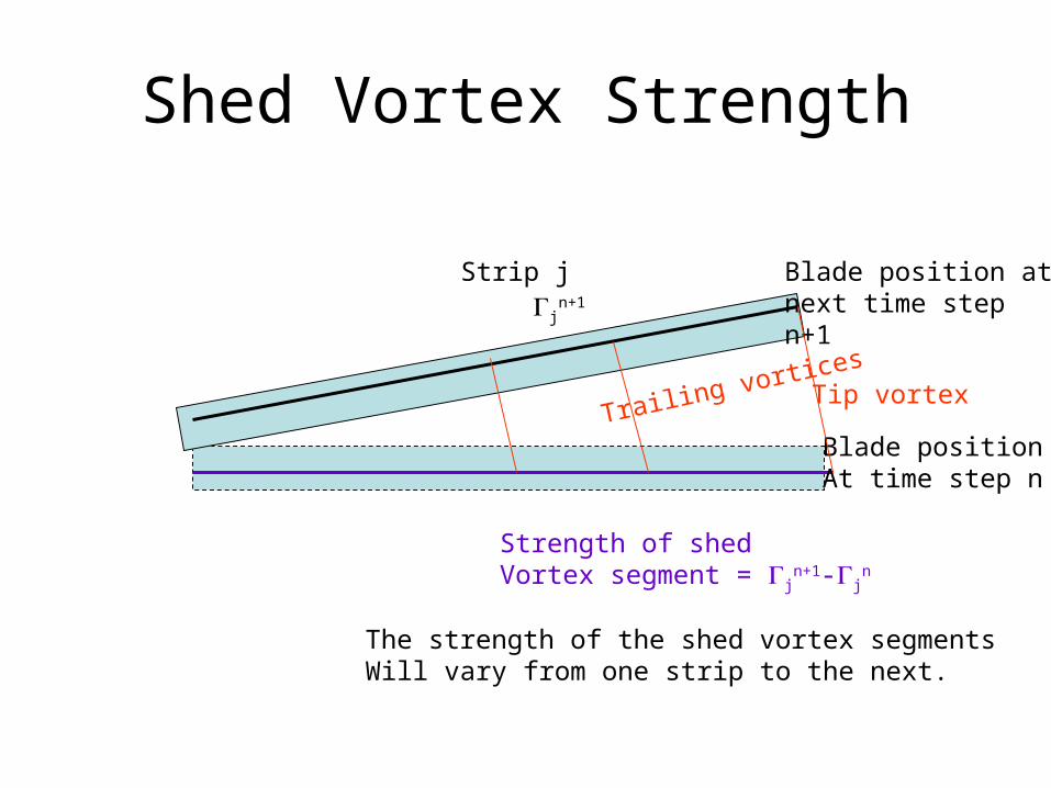
Shed Vortex Strength

Blade positionAt time step n

Blade position at next time stepn+1

jn+1

Strength of shedVortex segment = j

n+1-jn

Trailing vortices

The strength of the shed vortex segmentsWill vary from one strip to the next.

Tip vortex

Strip j

Induced Velocity Calculation

• The calculations are done in a time marching mode.

• The strength of the shed and trailing vortices are known from the previous time steps.

• The geometry of the wake is assumed to be a helix (rigid), prescribed (deformed wake, curve fitted from experiments) or free wake.

• Free wake geometry is computed by allowing the wake to move at the freestream velocity plus the induced velocity computed at the junction points (markers).

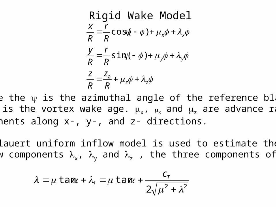
Rigid Wake Model

where the is the azimuthal angle of the reference blade, and is the vortex wake age. x, x and z are advance ratioComponents along x-, y-, and z- directions.

The Glauert uniform inflow model is used to estimate the inflow components x, y and z , the three components of .

222tantan

T

i

c

zz

yy

xx

R

z

R

zR

r

R

yR

r

R

x

0

)sin(

)cos(

Wake Age

Tip Vortex

x

zz

yy

xx

R

z

R

zR

r

R

yR

r

R

x

0

)sin(

)cos(

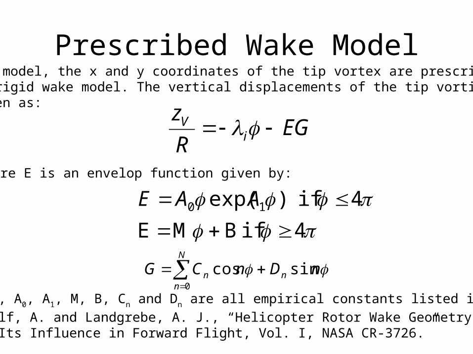
Prescribed Wake ModelIn this model, the x and y coordinates of the tip vortex are prescribed from a rigid wake model. The vertical displacements of the tip vortices are given as:

EGR

zi

V

where E is an envelop function given by:

4 if BME

4 if )exp( 10

AAE

N

nnn nDnCG

0

sincos

Here, A0, A1, M, B, Cn and Dn are all empirical constants listed in

“Egolf, A. and Landgrebe, A. J., “Helicopter Rotor Wake Geometry and Its Influence in Forward Flight, Vol. I, NASA CR-3726.”

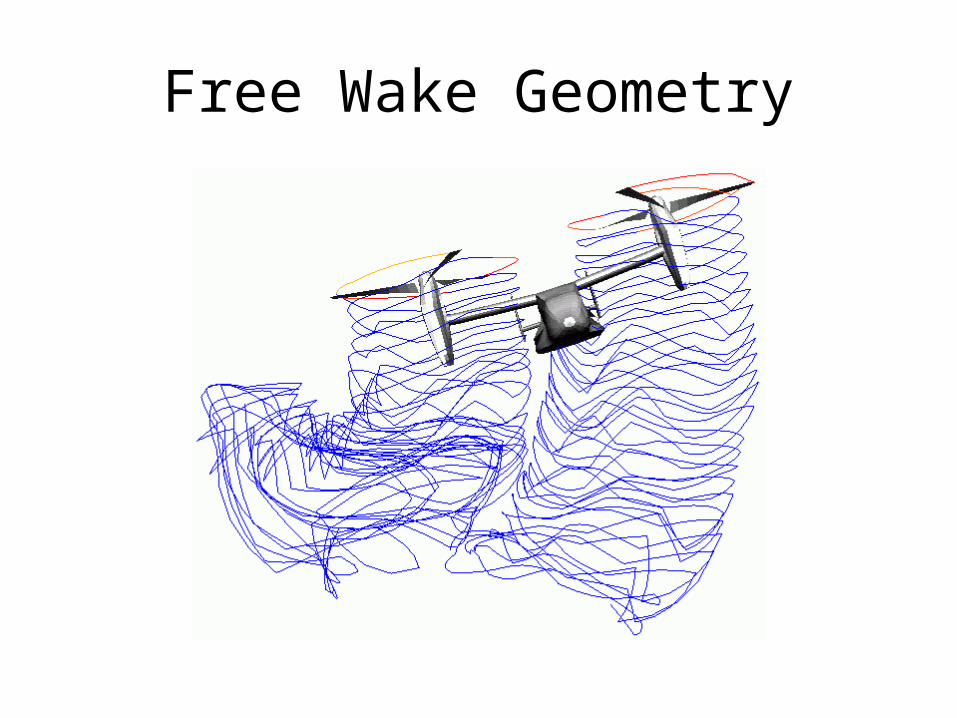
Free Wake Geometry