Embed Size (px)
Citation preview
Classical Mechanics
Babis Anastasioua, Vittorio del Ducab
Institute for Theoretical Physics, ETH Zurich,8093 Zurich, SwitzerlandaE-mail: [email protected]
bE-mail: [email protected]: Patrik Weber
December 17, 2015
Abstract
The subject of the course is classical mechanics. The followingtopics are discussed:
• Galileian transformations and Newtonian mechanics
• Variational methods
• Principle of least action
• Lagrangian mechanics
• Symmetries and conservation laws
• Two body systems
• Oscillations
• Rigid body dynamics
• Hamiltonian mechanics
• Hamilton-Jacobi equation
• Special Relativity
1
References[1] Landau and Lifshitz, Mechanics, Course of Theoretical Physics Vol. 1.,
Pergamon Press
[2] Classical Mechanics, 3rd Edition, Goldstein, Poole and Safko, AddisonWesley
[3] F. Gantmacher, Lectures in Analytical Mechanics, Mir Publications.
2
Contents1 Principle of relativity and Galileian transformations 6
1.1 Time intervals and distances in two inertial frames . . . . . . . 71.2 Vectors, scalars and rotations . . . . . . . . . . . . . . . . . . 71.3 The form of laws in classical mechanics . . . . . . . . . . . . . 10
2 Variational methods 122.1 The brachistochrone (βραχιστos χρoνos= shortest time) prob-
lem . . . . . . . . . . . . . . . . . . . . . . . . . . . . . . . . . 122.2 Euler-Lagrange equations . . . . . . . . . . . . . . . . . . . . . 132.3 Propagation of light . . . . . . . . . . . . . . . . . . . . . . . . 162.4 Solution of the brachistochrone problem . . . . . . . . . . . . 21
3 Hamilton’s principle of least action 243.1 The Lagrangian of a free particle in an inertial frame . . . . . 253.2 Lagrangian of a particle in a homogeneous force field . . . . . 273.3 Lagrangian of a system of particles with conserved forces . . . 293.4 Lagrangian for a charge inside an electromagnetic field . . . . 30
4 Dynamics of constrained systems 334.1 Constraints . . . . . . . . . . . . . . . . . . . . . . . . . . . . 334.2 Possible and virtual displacements . . . . . . . . . . . . . . . . 374.3 Smooth constraints . . . . . . . . . . . . . . . . . . . . . . . . 404.4 The general equation of the dynamics . . . . . . . . . . . . . . 434.5 Independent generalised coordinates . . . . . . . . . . . . . . . 444.6 Euler-Lagrange equations for systems with smooth constraints
and potential forces . . . . . . . . . . . . . . . . . . . . . . . . 45
5 Application of Euler-Lagrange equations: Simple pendulum 49
6 Minimization with Lagrange multipliers 536.1 Minimization of a multivariate function with Lagrange multi-
pliers . . . . . . . . . . . . . . . . . . . . . . . . . . . . . . . . 536.2 Minimizing the action with Lagrange multipliers . . . . . . . . 57
7 Conservation Laws 617.1 Conservation of energy . . . . . . . . . . . . . . . . . . . . . . 617.2 Conservation of momentum . . . . . . . . . . . . . . . . . . . 62
3
7.3 Angular momentum . . . . . . . . . . . . . . . . . . . . . . . . 657.4 Summary of conservation laws & symmetry . . . . . . . . . . 677.5 Conservation of generalized momenta . . . . . . . . . . . . . . 687.6 Noether’s Theorem . . . . . . . . . . . . . . . . . . . . . . . . 687.7 Noether’s theorem & time symmetries . . . . . . . . . . . . . 717.8 Continuous Symmetry Transformations . . . . . . . . . . . . . 73
8 Motion in one dimension 79
9 Two-body problem 829.1 1
rpotential . . . . . . . . . . . . . . . . . . . . . . . . . . . . . 89
9.2 Laplace-Runge-Lenz vector . . . . . . . . . . . . . . . . . . . . 949.3 Scattering . . . . . . . . . . . . . . . . . . . . . . . . . . . . . 97
9.3.1 Rutherford’s formula . . . . . . . . . . . . . . . . . . . 99
10 Virial Theorem 101
11 Oscillations 10411.1 Small Oscillations . . . . . . . . . . . . . . . . . . . . . . . . . 10411.2 Forced Oscillations . . . . . . . . . . . . . . . . . . . . . . . . 10611.3 Oscillations of systems with many degrees of freedom . . . . . 10911.4 Damped Oscillations . . . . . . . . . . . . . . . . . . . . . . . 112
12 Rigid Body 11512.1 Tensor of inertia . . . . . . . . . . . . . . . . . . . . . . . . . . 118
12.1.1 Examples of moments of inertia . . . . . . . . . . . . . 12012.2 Angular momentum . . . . . . . . . . . . . . . . . . . . . . . . 125
12.2.1 Precession . . . . . . . . . . . . . . . . . . . . . . . . . 12712.3 Equations of motion of rigid body . . . . . . . . . . . . . . . . 130
12.3.1 Applications: Free rotational motion . . . . . . . . . . 13412.3.2 Euler angles . . . . . . . . . . . . . . . . . . . . . . . . 136
13 Hamiltonian mechanics 13913.1 Hamilton equations . . . . . . . . . . . . . . . . . . . . . . . . 14013.2 The Hamiltonian as a conserved quantity and/or the total energy14513.3 Cyclic coordinates . . . . . . . . . . . . . . . . . . . . . . . . . 15013.4 Hamilton’s equations and Hamilton’s principle . . . . . . . . . 15213.5 Canonical transformations . . . . . . . . . . . . . . . . . . . . 15313.6 A canonical transformation for the harmonic oscillator . . . . 156
4
13.7 Canonical transformations in symplectic notation . . . . . . . 15813.8 Infinitesimal canonical transformations . . . . . . . . . . . . . 16113.9 Integrals of the equations of motion, Poisson brackets and
canonical invariants . . . . . . . . . . . . . . . . . . . . . . . . 16413.10Conservation theorems & canonical transformations through
the Poisson bracket . . . . . . . . . . . . . . . . . . . . . . . . 16913.11More on angular momentum and Poisson brackets . . . . . . . 17413.12Kepler problem in the Hamiltonian formalism . . . . . . . . . 17613.13Poincare (Cartan) integral invariants . . . . . . . . . . . . . . 178
14 Hamilton-Jacobi formalism 18614.1 Hamilton-Jacobi equation . . . . . . . . . . . . . . . . . . . . 18614.2 Simple harmonic oscillator . . . . . . . . . . . . . . . . . . . . 19114.3 2-dimensional harmonic oscillator . . . . . . . . . . . . . . . . 19214.4 Separation of variables . . . . . . . . . . . . . . . . . . . . . . 19314.5 Action-angle variables . . . . . . . . . . . . . . . . . . . . . . 195
15 Special Relativity 19715.1 Proper time . . . . . . . . . . . . . . . . . . . . . . . . . . . . 19715.2 Subgroups of Lorentz transformations . . . . . . . . . . . . . . 19915.3 Time dilation . . . . . . . . . . . . . . . . . . . . . . . . . . . 20115.4 Doppler effect . . . . . . . . . . . . . . . . . . . . . . . . . . . 20215.5 Particle dynamics . . . . . . . . . . . . . . . . . . . . . . . . . 20315.6 Energy and momentum . . . . . . . . . . . . . . . . . . . . . . 20515.7 The inverse of a Lorentz transformation . . . . . . . . . . . . . 20715.8 Vectors and Tensors . . . . . . . . . . . . . . . . . . . . . . . 208
5
1 Principle of relativity and Galileian transfor-mations
We will assume the existence of frames of reference (a system of coordinates)in which the motion of a free particle (on which no force is applied) is uniform,i.e. it moves with a constant velocity.
free particle: v = constant. (1.1)
Such reference frames are called inertial.The principle of relativity states that the laws of physics take the
exact same form in all inertial frames.Let us assume that we know the trajectory (position as a function of time)
of all the particles which constitute a physical system as they are observed inone inertial reference frame S. Can we compute the trajectories in a differentinertial frame S ′? To achieve that, we need to transform the space and timecoordinates (r, t) in the frame S to the corresponding coordinates (r′, t′) inthe frame S ′. A good guess for (Cartesian) coordinate transformations arethe so called Galilei transformations:
r′ = R r − r0 − V t, t′ = t0 + t. (1.2)
or, equivalently,
r′i =3∑j=1
Rijrj − r0,i − Vit. (1.3)
where V is the apparent velocity for a point in the frame S ′ according to anobserver in the frame S. r0 is the position of the origin of S ′ as seen in S ata time t = 0 and t0 is the time shown in the clock of S ′ at t = 0. The 3× 3matrix R describes the rotation of the axes of S ′ with respect to the axes ofS and it satisfies:
RTR = 13×3 , (1.4)
where 13×3 is the 3× 3 identity matrix. Equivalently, we write
RijRik = δjk, (1.5)
where δij is the Kronecker delta symbol. In addition, the determinant of therotation matrix is:
detR = 1. (1.6)
6
It turns out that Galileo’s transformations are only accurate for smallvelocities in comparison to the speed of light: V c. We will discussthe correct generalisation of Galileo’s transformations (the so called Lorentztransformations) towards the end of this course. In the mean time, we willassume that Eq 1.2 is valid; this is an excellent approximation for a plethoraof phenomena.
1.1 Time intervals and distances in two inertial frames
Consider two events:Event A: (tA, rA),
Event B: (tB, rB),
as observed in the reference frame S.In the reference frame S ′ these events are described by the time and space
coordinates:
Event A: (t′A, r′A) = (tA + t0,RrA + r0 − V tA),
Event B: (t′B, r′B) = (tB + t0,RrB + r0 − V tB).
The time difference of the two events is equal in the two frames S and S ′:
t′A − t′B = tA − tB. (1.7)
Therefore, time intervals are measured to be the same in all inertial frames.Space distances are also the same in all inertial frames. For two eventsoccurring at the same time t, their space distance is
∆r′ = |r′A − r′B| = |R rA −RrB| =√
(rA − rB)TRTR(rA − rB)
=√
(rA − rB)T (rA − rB) = |rA − rB| = ∆r. (1.8)
1.2 Vectors, scalars and rotations
The position of a particle r, under a rotation, transforms as:
r → r′ = R r, detR = 1, RTR = 1. (1.9)
The position is one of many other objects with the same transformationunder rotations. We can formally define a vector A to be a set of three
7
numbers which transforms in the same way as the position vector does undera rotation:
A→ A′ = RA, detR = 1, RTR = 1. (1.10)
For example, time derivatives of the position vector (velocity, acceleration,. . .) are also vectors:
dr
dt→ dr′
dt′=d(R r)
dt= R
dr
dt(1.11)
We can define a dot-product of two vectors as
A ·B =3∑i=1
AiBi. (1.12)
The dot product is invariant under rotations:
A ·B → A′ ·B′ =∑i
A′iB′i =
∑ijk
(RijAj)(RikBk)
=∑ijk
RTjiRikAjBk =
∑jk
δjkAjBk =∑k
AkBk
= A ·B. (1.13)
All objects which are invariant under rotation transformations are calledscalars.
The cross-product of two vectors (such as the angular momentum) is alsoa vector. Indeed, if A,B are vectors then their cross-product transforms as:
A×B → A′ ×B′ = R(A×B). (1.14)
To prove the above, consider the dot product
(A×B) · C =∑i
(∑jk
εijkAjBk
)Ci = det
(A , B , C
)Under a rotation, this dot product is invariant,
det(A , B , C
)→ det
(A′ , B′ , C ′
)= det
(RA , RB , RC
)= det
R(A , B , C
)= det(R) det
(A , B , C
)= det
(A , B , C
)(1.15)
8
and it is therefore a scalar:
(A′ ×B′) · C ′ = (A×B) · C; (A′ ×B′) · (RC) = (A×B) · C
;
[RT (A′ ×B′)
]· C = (A×B) · C
; (A′ ×B′) · C =[R (A×B)
]· C (1.16)
Since the above is valid for any vector C, we conclude that
A′ ×B′ = R (A×B). (1.17)
Finally, the gradient differential operator
∇ ≡(
∂
∂x1
,∂
∂x2
,∂
∂x3
)(1.18)
is also a vector. To see this, we first note that
x′i =∑j
Rijxj ;∂x′i∂xj
= Rij (1.19)
andxi =
∑j
RTijx′j ;
∂xi∂x′j
= RTij = Rji. (1.20)
Then∇ → ∇′ = ∂
∂x′i=∑j
∂xj∂x′i
∂
∂xj=∑j
Rij∂
∂xj= R∇. (1.21)
The rotation matrix R is a particular case of a Jacobian matrix, in thiscase the one for a change of variables. In general, given a vector-valuedfunction, f : Rn → Rm which maps a vector x ∈ Rn onto a vector f(x) ∈Rm, that is, given m functions, f1, . . . , fm, each depending on n variables,x1, . . . , xn, the Jacobian matrix is defined as,
Jij =∂fi∂xj
, i = 1, . . . ,m , j = 1, . . . , n . (1.22)
Note that the gradient (1.18) is the particular case of a Jacobian matrix withm = 1.
9
Jacobian matrices are also needed to invert functions. In fact, noting thata function is continuously differentiable if its derivative is also a continuousfunction, a vector-valued function is continuously differentiable if the entriesof the Jacobian matrix are continuous functions. If m = n, we can define thedeterminant of the Jacobian matrix, usually called the Jacobian,
|Jij| =∣∣∣∣ ∂fi∂xj
∣∣∣∣ , i, j = 1, . . . , n .
The inverse function theorem states that if a continuously differentiable func-tion f : Rn → Rn has a non-vanishing Jacobian at a point x, then f is in-vertible near x, and the inverse function is also a continuously differentiablefunction.
1.3 The form of laws in classical mechanics
The Galileian principle of relativity requires that all laws of physics are thesame in inertial reference frames. If we can cast our physics laws as vectorequalities, it is then guaranteed that they will have the same form for allframes which are related by a rotation transformation.
Physics law in frame S: A = B
; RA = RB
; Physics law in frame with rotated axes S ′: A′ = B′ (1.23)
The principle of relativity requires that the laws of physics take the sameform not only under rotation transformations but also under “boosts” wheretwo reference frames appear to move with a relative velocity with respect toeach other:
r → r′ = r + V t (1.24)
Notice that the acceleration vector
a ≡ d2r
dt2=d2r′
dt2= a′ (1.25)
is the same for all inertial observers with parallel axes. Newton’s law:
F = ma (1.26)
10
connects the acceleration, a boost invariant quantity, to the force. As longas the latter is also boost invariant then the Galileian principle of relativityis satisfied.
You will soon figure out that the acceleration vector is not boost invariantwhen using the correct principle of relativity as it is formulated in Einstein’sspecial relativity. Therefore, we should not expect that the physical forces ofnature are boost invariant either. Having said that, we will be able to ignorespecial relativity in most of our classical mechanics investigations, in the sameway that Newton and many others were oblivious about it when they set thefoundations of modern physics. In particular, our Newtonian understandingof gravity is consistent with the Galileian principle of relativity.
Consider an isolated system of N-particles which interact with each otherthrough the gravitational force only. The force acting on the i-th particle ina reference frame S is
mid2ridt2
= −G∑j 6=i
mimjri − rj|ri − rj|3
(1.27)
According to the principle of relativity, a Galileian transformation
(t, r)→ (t′, r′) = (t+ t0,R r + V t+ r0)
should leave Eq. 1.27 invariant. Indeed, this is satisfied. In the new frame,
mid2ri
′
dt′2= −G
∑j 6=i
mimjri′ − rj ′
|ri′ − rj ′|3
; Rmid2ridt2
= −RG∑j 6=i
mimjri − rj|ri − rj|3
; mid2ridt2
= −G∑j 6=i
mimjri − rj|ri − rj|3
(1.28)
Question: Is the electromagnetic force boost invariant?
11
2 Variational methodsClassical mechanics is usually formulated in terms of Newton’s laws in theform of second order differential equations as in Eq. 1.27. There is an al-ternative, where we can formulate the laws of classical mechanics by meansof the so called variational principle. It is based on a scalar quantity, calledthe action. Before we present this formulation, let us warm up with a fewphysics and mathematics problems in using variation calculus techniques.
2.1 The brachistochrone (βραχιστos χρoνos = shortesttime) problem
x
z(xa, za)
(xb, zb)
~v
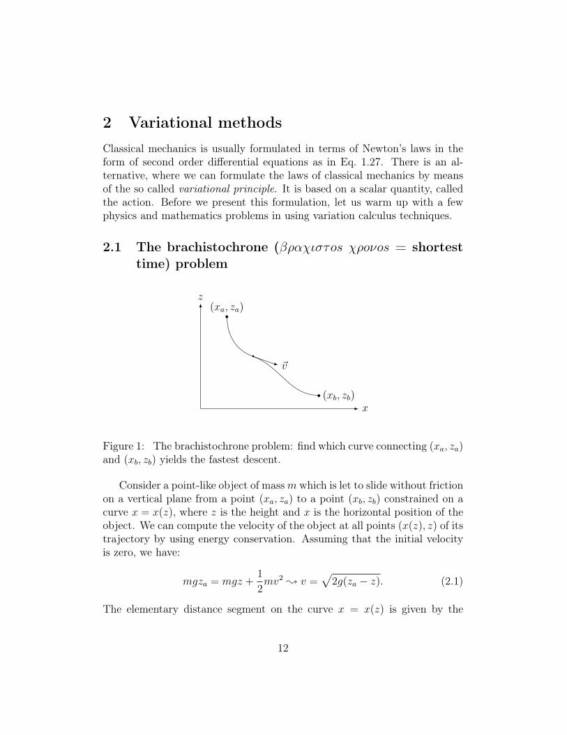
Figure 1: The brachistochrone problem: find which curve connecting (xa, za)and (xb, zb) yields the fastest descent.
Consider a point-like object of massm which is let to slide without frictionon a vertical plane from a point (xa, za) to a point (xb, zb) constrained on acurve x = x(z), where z is the height and x is the horizontal position of theobject. We can compute the velocity of the object at all points (x(z), z) of itstrajectory by using energy conservation. Assuming that the initial velocityis zero, we have:
mgza = mgz +1
2mv2 ; v =
√2g(za − z). (2.1)
The elementary distance segment on the curve x = x(z) is given by the
12
Pythagorean theorem as:
ds =√dx2 + dz2 = dz
√1 +
(dx
dz
)2
(2.2)
and the magnitude of the velocity is
v =ds
dt; dt =
ds
v= dz
√1 +
(dxdz
)2
2g(za − z)(2.3)
The total time for the transition is:
T =
∫dt =
∫ zb
za
dz
√1 +
(dxdz
)2
2g(za − z)(2.4)
We are seeking the function x(z) which minimizes the time T .
2.2 Euler-Lagrange equations
The problem that we have just described above belongs to a more gen-eral class of variational calculus problems. We seek to find which functiony(t) = ys(t) among all good-behaved functions y(t) yields an extreme value(minimum or maximum) for the integral
I[y] =
∫ tb
ta
dtF (y(t), y′(t)) (2.5)
given that the values of the function at the initial and final points in theintegration domain y(ta) = ya, y(tb) = yb are known.
Assume that we have found the curve ys(t) with
ys(ta) = ya, ys(tb) = yb (2.6)
for which I[ys] is a minimum of I[y] 1. Consider now a small deformationaround ys(t)
y(t) = ys(t) + δys(t) , δys(t) = εη(t), ε→ 0 , (2.7)1Notice that I[y] is an integral function of a function. Such integrals are usually called
functionals
13
where η(t) is a smooth function which vanishes at the boundaries
η(ta) = η(tb) = 0, (2.8)
in order to satisfy that y(ta) = ya, y(tb) = yb. Since I[ys] is an extremum,we must have that our small deformation (ignoring O(ε2) terms) does notchange its value,
I[ys] = I[ys + δys]
=
∫ tb
ta
dt F (ys(t) + δys(t), y′s(t) + δy′s(t)) . (2.9)
We observe that the operations of varying a function and taking its derivativewith respect to its argument commute:
δy′s(t) =d
dtδys(t) = εη′(t) (2.10)
Thus we can Taylor expand the arguments of F , and write
I[ys] =
∫ tb
ta
dt F (ys(t), y′s(t)) +
∫ tb
ta
dt
[∂F
∂ysεη(t) +
∂F
∂y′sεη′(t)
]+O(ε2)
= I[ys] + ε
∫ tb
ta
dt
[∂F
∂ysη(t) +
∂F
∂y′sη′(t)
]+O(ε2) (2.11)
This yields that
0 =
∫ tb
ta
dt
[∂F
∂ysη(t) +
∂F
∂y′sη′(t)
]=
∫ tb
ta
dt
[∂F
∂ys− d
dt
∂F
∂y′s
]η(t) +
∫ tb
ta
dtd
dt
[∂F
∂y′sη(t)
]=
∫ tb
ta
dt
[∂F
∂ys− d
dt
∂F
∂y′s
]η(t) +
∂F
∂y′sη(t)
∣∣∣∣tbta
dt (2.12)
The last term is zero due to η(t) vanishing on the boundaries. Thus, theintegral ∫ tb
ta
dt
[∂F
∂ys− d
dt
∂F
∂y′s
]η(t) = 0 (2.13)
14
vanishes for every function η(t). In order for this to happen, we must have:
∂F
∂ys− d
dt
∂F
∂y′s= 0. (2.14)
This is the Euler-Lagrange equation.A completely analogous derivation of Euler-Lagrange differential equa-
tions can be made for minimising multidimensional integrals which are func-tionals of many functions. Given a vector-valued function, y : Rn → Rm
which maps a vector x ∈ Rn onto a vector y(x) ∈ Rm, that is, given m func-tions, y1, . . . , ym, each depending on n variables, x1, . . . , xn, we may considerthe integral,
I[y1, . . . , ym] =
∫dx1 . . . dxnF
[yi(x),
∂yi(x)
∂xj
]. (2.15)
Requiring that the above integral takes a minimum or maximum value undersmall variations of the functions
yi(x)→ yi(x) + δyi(x) = yi(x) + εηi(x) , i = 1, . . . ,m ,
the integral value should be unchanged:
0 = δI[y1, . . . , ym]
= δ
∫dx1 . . . dxnF
[yi(x),
∂yi(x)
∂xj
]=
∫dx1 . . . dxn
[m∑i=1
∂F
∂yiδyi(x) +
m∑i=1
n∑j=1
∂F
∂(∂jyi)δ∂jyi(x)
], (2.16)
where we have introduced the shorthand notation,
∂j ≡∂
∂xj.
We use again that the operations of varying a function and taking its deriva-tive with respect to its arguments commute:
δ∂jyi(x) = ∂jδyi(x) (2.17)
15
and after performing integration by parts, we have
0 = ε
∫dx1 . . . dxn
m∑i=1
ηi
[∂F
∂yi−
n∑j=1
∂j∂F
∂(∂jyi)
]
+ε∑ij
∫dx1 . . . dxm∂j
[ηi
∂F
∂(∂jyi)
]. (2.18)
The second term is a total derivative in the xj integration and it vanishes byrequiring that the variations yi(x) vanish at the boundaries of the integration.Since the above identity must be valid for an arbitrary choice of functionsηi(x) we arrive at the general Euler-Lagrange equations:
∂F
∂yi−
n∑j=1
∂j∂F
∂(∂jyi)= 0 , i = 1, . . . ,m . (2.19)
A particularly useful case is the one of a vector-valued function of one vari-able, y : R → Rm which maps a variable x ∈ R onto a vector y(x) ∈ Rm,that is, the case treated above with n = 1. Then the general Euler-Lagrangeequations become
∂F
∂yi− d
dx
∂F
∂y′i= 0 , i = 1, . . . ,m . (2.20)
2.3 Propagation of light
Equipped with the Euler-Lagrange equations (2.20) we consider the propa-gation of light. Fermat formulated the homonymous principle, stating thatlight travels from point to point choosing the path which yields the fastesttime. For such a transition, the total time is
T =
∫dt =
∫ds
v(x), (2.21)
where ds is the distance element and v(x) is the speed of light at the pointx. This is usually normalised to the speed of light in the vacuum c,
v(x) =c
n(x), (2.22)
16
where n(x) is the refraction index. Fermat’s principle requires that
T =1
c
∫ds n(x) =
1
c
∫ √dx2 + dy2 + dz2n(x)
=1
c
∫dx
√1 +
(dy
dx
)2
+
(dz
dx
)2
n(x) (2.23)
is a minimum.Let us assume that the index of refraction is a constant,
n(x) = n = const.
Then
T =n
c
∫dx
√1 +
(dy
dx
)2
+
(dz
dx
)2
. (2.24)
Formally, we can write it as,
T [y, z] =
∫dxF (y′(x), z′(x)) (2.25)
withF (y′(x), z′(x)) =
n
c
√1 + y′2(x) + z′2(x) . (2.26)
Note that F does not depend explicitly on y and z.The Euler-Lagrange equations read:
∂F
∂y− d
dx
∂F
∂y′= 0
∂F
∂z− d
dx
∂F
∂z′= 0 . (2.27)
Then computing the derivatives,
∂F
∂y= 0 ,
∂F
∂y′=n
c
y′√1 + y′2 + z′2
∂F
∂z= 0 ,
∂F
∂z′=n
c
z′√1 + y′2 + z′2
(2.28)
17
the Euler-Lagrange equations become,
d
dx
y′√1 + y′2 + z′2
= 0
d
dx
z′√1 + y′2 + z′2
= 0 , (2.29)
which can be trivially integrated,
y′√1 + y′2 + z′2
= c1
z′√1 + y′2 + z′2
= c2 , (2.30)
where c1 and c2 are constants. The solution of these equations is a straightline.
Hint: In order to see it, solve first the simpler case of a light ray in thex− y plane. Then the Euler-Lagrange equation is
d
dx
y′√1 + y′2
= 0 (2.31)
which is integrated toy′√
1 + y′2= c (2.32)
where c is a constant. This can be solved in y′,
y′ = ± c√1− c2
= a (2.33)
where a is a constant. Integrating it, we get the equation of a straight line
y(x) = ax+ b . (2.34)
Likewise, the coupled system (2.30) can be solved to find that
y(x) = a1x+ b1
z(x) = a2x+ b2 . (2.35)
which are the parametric equations of a straight line.
18
n1
n2
θI
A
θR
B
θT
C
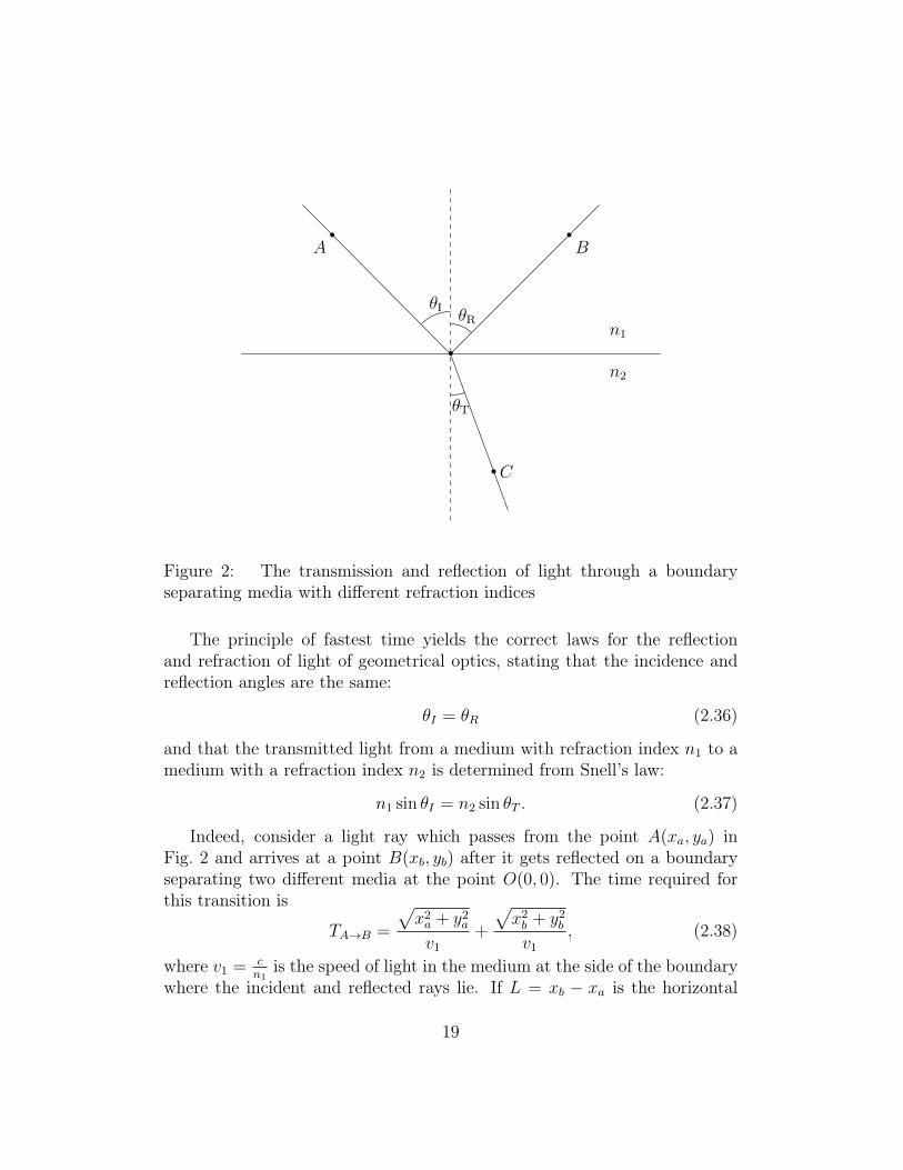
Figure 2: The transmission and reflection of light through a boundaryseparating media with different refraction indices
The principle of fastest time yields the correct laws for the reflectionand refraction of light of geometrical optics, stating that the incidence andreflection angles are the same:
θI = θR (2.36)
and that the transmitted light from a medium with refraction index n1 to amedium with a refraction index n2 is determined from Snell’s law:
n1 sin θI = n2 sin θT . (2.37)
Indeed, consider a light ray which passes from the point A(xa, ya) inFig. 2 and arrives at a point B(xb, yb) after it gets reflected on a boundaryseparating two different media at the point O(0, 0). The time required forthis transition is
TA→B =
√x2a + y2
a
v1
+
√x2b + y2
b
v1
, (2.38)
where v1 = cn1
is the speed of light in the medium at the side of the boundarywhere the incident and reflected rays lie. If L = xb − xa is the horizontal
19
distance with the two points, then we write:
cTA→B = n1
√x2a + y2
a + n1
√(L+ xa)2 + y2
b (2.39)
Requiring the above to be a minimum, we find that the horizontal positionxa must satisfy
∂TA→B∂xa
= 0
;xa√x2a + y2
a
+(L+ xa)√
(L+ xa)2 + y2b
= 0
; − sin θI + sin θR = 0 , (2.40)
which yields that the incident and reflected light angles are the same,
θI = θR. (2.41)
Repeating the same steps for a transition from the point A inside the mediumwith a refraction index n1 to a point C inside the medium with refractionindex n2,
∂TA→C∂xa
= 0
; n1xa√x2a + y2
a
+ n2(L+ xa)√
(L+ xa)2 + y2c
= 0
; −n1 sin θI + n2 sin θT = 0 , (2.42)
we find Snell’s law,n1 sin θI = n2 sin θT . (2.43)
Interesting phenomena occur when the index of refraction is not uniform.For example, the atmospheric air density changes with the temperature. Thenon-uniformity of the density is responsible for for interesting phenomena,such as mirage images in deserts or on the surface of a hot road in thesummer and the twinkling of stars. In such media, the trajectory of the lightis not a straight line.
20
2.4 Solution of the brachistochrone problem
We can return now to the problem of subsection 2.1. The functional T ofEq. 2.4 can be written as
T [x] =
∫ zb
za
dzF (x′(z)) (2.44)
with
F =
√1 + x′2(z)
2g(za − z)(2.45)
Note that F does not depend explicitly on x.Requiring that the functional (2.44) be a minimum, we can write the
Euler-Lagrange equation 2.14
∂F
∂x− d
dz
∂F
∂x′= 0. (2.46)
Performing the differentiations,
∂F
∂x= 0 ,
∂F
∂x′=
x′√2g(za − z)(1 + x′2(z))
, (2.47)
we obtain the second order differential equation:
d
dz
x′√(za − z)(1 + x′2)
= 0 (2.48)
which, after a trivial first integration, gives:
x′√(za − z)(1 + x′2)
= −C, (2.49)
with C a constant to be fixed by our boundary conditions. Solving for x′, weobtain:
x′2
=C2(za − z)
1− C2(za − z)(2.50)
For the rhs to be a positive definite variable, we must have either
z ≥ za and C2(za − z) ≥ 1,
21
orz ≤ za and C2(za − z) ≤ 1.
The first possibility is not physically allowed, since it is not satisfied by thefinal point (xb, zb) which lies lower than (xa, za).
Let’s now change variables:
C2(za − z) = sin2 φ, φ ∈[0,π
2
](2.51)
withdz
dφ= − 1
C2sin(2φ). (2.52)
The differential equation for x(φ) becomes:
dx
dφ= 2
C
|C|3sin2 φ (2.53)
It is now straightforward to perform the integrations over φ and computex = x(φ), z = z(φ). We can choose that φ = 0 corresponds to the first point(xa, za) of the curve. This gives the solutions:
x(φ) = xa +C
2|C|3[2φ− sin(2φ)] (2.54)
z(φ) = za −1
2C2[1− cos(2φ)] (2.55)
Setting φ = θ/2 with θ ∈ [0, π], we have
x(θ) = xa +C
2|C|3[θ − sin θ] (2.56)
z(θ) = za −1
2C2[1− cos θ] (2.57)
Choosing a positive value for C we obtain solutions where the curve lies tothe right of the starting point (as in Figure 1) while for C < 0 we obtainsolutions where the curve lies to the left of the starting point. For C > 0 wehave
x(θ) = xa +1
2C2[θ − sin θ] (2.58)
22
z(θ) = za −1
2C2[1− cos θ] (2.59)
These are the equations of a cycloid. To determine the constant C2 werequire that the final point (xb, zb) belongs to the curve, i.e. there exists avalue θ = θb such that
xb = xa +1
2C2[θb − sin θb] (2.60)
zb = za −1
2C2[1− cos θb] (2.61)
For any specific value of the pairs (xa, za) and (xb, zb) one can use eqs. (2.60)and (2.61) to determine numerically θb and C, and from this the radius ofthe cycle generating the required cycloid curve,
r =1
2C2(2.62)
Exercise 2.1. Determine C and r for (xa, za) = (0, 1) and (xb, zb) = (2, 0).
You can find a nice demonstration of the brachistochrone problem in thisvideo.
23
3 Hamilton’s principle of least actionAfter the observation that the behaviour of light can be understood by meansof a “least time principle” and variational techniques, the question ariseswhether variational methods can also be used more generally for the studyof physical systems.
The main result of variational methods is the Euler-Lagrange differen-tial equations. The laws of classical physics, Newton’s laws and Maxwellequations of electrodynamics were first discovered in the form of differentialequations. The question we are posing here is a reverse-engineering prob-lem. If we know the Euler-Lagrange equations (physics laws in differentialequations form) can we find the integral functional from which they arise?Hamilton’s principle of least action states that this is possible.
Consider an isolated system of many particles i = 1 . . . N for which wewould like to know their trajectories, i.e their positions at all times. While itis common to use Cartesian coordinates, ri(t), it is often useful to use othervariables such as angles, radii, or even more exotic variables to describe thetrajectory of a particle. We call these generic variables which describe atrajectory as generalised coordinates.
Assume now that we know at an initial time ti the values of a set ofindependent generalised coordinates
q1(ti), . . . , qm(ti)
as well as the initial values of their time derivarives (generalised velocities)
·q1 (ti), . . . ,
·qm (ti).
Hamilton’s principle of least action states that the generalised coordinatesand generalised velocities of the system are determined at a later time tf byrequiring that action:
S ≡∫ tf
ti
dt L[qj(t),
·qj (t)
](3.1)
is minimum:δS = 0. (3.2)
The integrand L of the action is called the Lagrangian. The Euler-Lagrangeequations derived from the principle of least action for physical systems are
24
called equations of motion and are given:
d
dt
∂L
∂·qi− ∂L
∂qi= 0. (3.3)
We note that the Lagrangian of a system is not uniquely defined. Considertwo Lagrangians L,L′ which differ by a total derivative:
L′ = L+df
dt, (3.4)
where f is an arbitrary function. The corresponding actions
S ′ =
∫ tf
ti
dt L′ =
∫ tf
ti
dt L+
∫ tf
ti
dtdf
dt= S + f(tf )− f(ti) (3.5)
differ by a constant which vanishes upon taking a variation of the generalisedcoordinates:
δS ′ = δS + δ (f(tf )− f(ti)) = δS. (3.6)
Therefore, Lagrangians which differ by a total derivative yield the same equa-tions of motion.
3.1 The Lagrangian of a free particle in an inertial frame
We will now find Lagrangians which govern known physical systems, startingfrom the simplest case. This is a free isolated particle (does not interact withother particles) which is observed in an inertial frame. The equation ofmotion of the particle is given by
a = 0, (3.7)
where the acceleration of the free particle is
a ≡ r =(··r1,··r2,··r3
). (3.8)
The Lagrangian:
L =1
2mv2 =
1
2m
3∑i=1
·r
2
i , (3.9)
25
yields the correct equation of motion:
0 =d
dt
∂L
∂·ri− ∂L
∂ri= m
··ri;
··ri= 0. (3.10)
Could we have guessed a different Lagrangian, which results to the acceler-ation being zero for a freely moving particle? For example, a Lagrangian:
L = (v2)n (3.11)
yields the equations of motion ( ·r
2
i
)n−1 ··ri= 0. (3.12)
For n 6= 1, in a rest frame where the particle is moving at a certain momentwith a velocity r 6= 0, we find that the acceleration must be zero. Never-theless, such equations of motion do not conform with Galileo’s principle ofrelativity which requires that under, for example, a boost
r → r′ = r + vt, (3.13)
Eq. 3.12 must maintain the same form, i.e.( ·r′2i
)n−1 ··ri′= 0. (3.14)
It does not, except for n = 1! Instead, one finds a frame dependent form:( ·r
2
i
)n−1 ··ri= 0
ri→r′i;
((·r′i −vi)2
)n−1 ··ri′= 0. (3.15)
A comment is appropriate on the constant factor m2in the Lagrangian of
the free particle of Eq. 3.9. Obviously, this factor is immaterial in derivingthe equations of motion. However, we will soon extend the Lagrangian toaccount for interactions with other particles. When this happens, we willassociate m with the physical mass of the particle. The principle of leastaction tells us that the physical mass is a positive quantity m > 0. Indeed,the general solution of the equations of motion is:
r = 0 ; r(t) = A+Bt. (3.16)
26
We can fix the constants A,B for a given transition from a space-time point(ti, ri) to a space-time point (tf , rf ). Then, the physical trajectory is givenby
rphys(t) = ri +t− titf − ti
(rf − ri) . (3.17)
The value of the action for the physical trajectory is
S [rphys(t)] =
∫ tf
ti
dtL[rphys(t)] =1
2m
(rf − ri)2
tf − ti. (3.18)
According to the principle of least action, any other trajectory than thephysical that we can think of to join the space-time points (ti, ri) and (tf , rf )should yield a value for the action which is greater. Consider, for example anon-physical trajectory:
rnon−phys(t) = ri +
(t− titf − ti
)2
(rf − ri) . (3.19)
It must beS [rnon−phys(t)]− S [rphys(t)] > 0. (3.20)
An explicit calculation shows that
S [rnon−phys(t)] =
∫ tf
ti
dtL[rnon−phys(t)] =2
3m
(rf − ri)2
tf − ti=
4
3S [rphys(t)] .
(3.21)Eq. 3.20 leads to the conclusion that the value of the action for the physicaltrajectory must be positive:
S [rphys(t)] =1
2m
(rf − ri)2
tf − ti> 0 (3.22)
and, since tf > ti, we must have that the mass is positive m > 0.
3.2 Lagrangian of a particle in a homogeneous forcefield
Consider a particle subjected to a constant force F . According to Newton’slaw, the equation of motion is
mr − F = 0, (3.23)
27
or, in components,m··ri −Fi = 0. (3.24)
As for the earlier case of the free particle, the first term of the above equationcan be written as
m··ri=
d
dt
∂T
∂·ri, (3.25)
whereT =
1
2m·r
2, (3.26)
the kinetic energy of the particle. We can write the second term as a deriva-tive:
Fi =∂(Firi)
∂ri=
∂
∂ri
3∑j=1
Fjrj = −∂(−F · r)∂ri
(3.27)
The dot product −F ·r is the work done against the force to bring the particlefrom the origin of our reference frame to the position r, or in other wordsthe potential energy of the particle:
U(r) = −F · r. (3.28)
Therefore, Newton’s law for a constant force takes the form:
d
dt
∂T
∂·ri− ∂(−U)
∂ri= 0. (3.29)
Given that the potential energy U does not depend on velocities·ri and that
the kinetic energy T does not depend on positions, we can rewrite the aboveequation as:
d
dt
∂(T − U)
∂·ri
− ∂(T − U)
∂ri= 0. (3.30)
This has taken the form of Euler-Lagrange equations,
d
dt
∂L
∂·ri− ∂L
∂ri= 0. (3.31)
where the LagrangianL = T − U (3.32)
is the difference of the kinetic and potential energy of the particle. While wehave derived this result for a constant force F , we shall see that it is moregeneral.
28
3.3 Lagrangian of a system of particles with conservedforces
Consider an isolated system of N -particles, i.e. particles which interact onlywith each other. We will postulate that the Lagrangian of the system is thedifference of the kinetic energy of the particles and the potential energy ofthe system:
L =∑a
1
2mar
2a − U (r1, . . . , rn) . (3.33)
The Euler-Lagrange equations for this Lagrangian read:
d
dt
∂L
∂·ra,i
=∂L
∂ra,i, (3.34)
where ra,i denotes the i−th component of the vector ra denoting the positionof the a−the particle. Performing the differentiations we obtain:
ma··ra,i= −
∂U
∂ra,i(3.35)
or, in vector notation,mra = −∇aU (3.36)
with ∇a ≡ (∂/∂ra,1, ∂/∂ra,2, ∂/∂ra,3). This is the known equation of motionaccording to Newton’s law for a conserved force, i.e. a force which can bewritten as the gradient of a potential:
Fa = −∇aU. (3.37)
As an example consider an isolated system of N particles with massesma which interact among themselves gravitationally. The Lagrangian of thesystem is
L = T − U (3.38)
where
T =N∑a=1
1
2mara (3.39)
andU = −1
2
∑a
∑b6=a
Gmamb
|ra − rb|(3.40)
29
The Euler-Lagrange equations are:
mara = −∇aU, (3.41)
where the subscript in ∇a denotes that the differentiations are made withrespect to the coordinates of the a-th particle.
Exercise 3.1. To carry out the differentiations in the rhs, we first provethat:
∇a1
|ra − rb|= − ra − rb|ra − rb|3
. (3.42)
We then obtain the equations of motion:
mara = −∑b6=a
Gmambra − rb|ra − rb|3
, (3.43)
in agreement with Newton’s law of gravitation.
3.4 Lagrangian for a charge inside an electromagneticfield
We now turn our attention to the force experienced by an electric chargewhich is in the vicinity of other electric charges. We can sum up the effectsof all other charges into two vectors:
• E(t, r), the electric field and
• B(t, r), the magnetic field.
The force is then given by:
mr = q(E + r ×B
), (3.44)
where m is the mass of the charge q. The electric and magnetic fields aredetermined from the equations of Maxwell:
∇ · E =ρ
ε0, (3.45)
∇× E = −∂B∂t, (3.46)
∇ ·B = 0, (3.47)
∇×B =j
c2ε0+
1
c2
∂E
∂t.(3.48)
30
where ρ(r) is the electric charge density and j is the electric current density.ε0 is a constant, the so-called vacuum permittivity, and has the value
ε0 = 8.854187817 . . . 1012 A · sVolt ·m
. (3.49)
c is the speed of light
c = 2.99792458 . . . 108m
s. (3.50)
We will not attempt here to find explicit solutions of Maxwell equationsfor the E and B fields, but we will assume that such solutions exist andare known to us. Can we obtain the equation of motion Eq. 3.44 fromHamilton’s variational principle? Unlike the example that we have seen sofar, the electormagnetic force depends not only on the position of the chargedparticle but also its velocity. Nevetheless, we will be able to find a Lagrangianwhich gives the correct equation of motion.
To achieve that, we introduce first the scalar and vector potentials, φ(t, r)and A(t, r) respectively, defined as:
E = −∂A∂t−∇φ (3.51)
B = ∇× A (3.52)
You can easily verify that the second and third of Maxwell equations areautomatically satisfied if we substitute the electric and magnetic field withthe scalar and vector potentials. Consider now the Lagrangian:
L =1
2mr
2 − qφ+ qr · A. (3.53)
Euler-Lagrange equations give the form
m··ri +q
dAidt
= −q∂iφ+ q∑j
·rj ∂iAj, (3.54)
where we use the shorthand notation
∂i ≡∂
∂ri.
31
The total time derivative of the vector potential is:
dAidt
=∂Ai∂t
+∑j
·rj (∂jAi) (3.55)
Then, Euler-Lagrange equations take the form
m··ri = q
[−∂Ai∂t− ∂iφ
]+ q
∑j
[ ·rj ∂iAj−
·rj (∂jAi)
]. (3.56)
In the first bracket, we recognize the i-th component of the electric field:
−∂Ai∂t− ∂iφ = Ei (3.57)
The second bracket is not as obvious to decipher, but we can prove it tobe the i-th component of the cross-product of the velocity and the magneticfield. Indeed
(r ×B)i =[r ×
(∇× A
)]i
=∑jklm
εijk·rj (εklm∂lAm)
=∑jlm
(δilδjm − δjlδim)·rj ∂lAm
=∑j
[ ·rj ∂iAj−
·rj (∂jAi)
]. (3.58)
Thus, we have proven that the Euler-Lagrange equations of the Lagrangianof Eq. 3.53 give the known Lorentz equation for the force of a charge insidean electromagnetic field:
m··ri= qEi + q
(r ×B
)i
(3.59)
32
4 Dynamics of constrained systemsIn the last section, we showed the equivalency of traditional Newtonian me-chanics and Hamilton’s variational principle for a variety of forces acting onsystems of particles. In this section, we will show that the principle of leastaction can be applied to dynamical systems for which we do not have a pri-ori knowledge of all forces acting on the particles but for some of them weonly know their effect in limiting the allowed motion of the particles. Forexample, particles which make up a ball are constrained to be kept togetherwith electromagnetic forces. It is difficult to account for these microscopicelectromagnetic interactions in our Lagrangian when our aim is simply todescribe the motion of the ball inside the gravitational field. However, ina variety of problems with constraints an explicit description of the forcesresponsible for the constraints can be avoided and we can implement directlytheir effect.
4.1 Constraints
The configuration of a system ofN particles Pj is given by the positions rj andthe velocities rj of the N particles. If all possible configurations are allowed,the system is free. If there are limitations to the possible configurations, themotion of the system is constrained. The geometric or kinematic restrictionsto the positions rj of the particles of the system are called constraints.
We will study a class of constraints which limit the positions and/or thevelocities of the particles, through equations of the form
f(r1, . . . , rN , r1, . . . , rN , t) = 0 . (4.1)
We call these constraints differential. If a differential constraint can be castin a form that it does not depend explicitly on the velocities, it is calledholonomic,
f(r1, . . . , rN , t) = 0 , (4.2)
thus it will limit only the positions of the particles. If, in particular, aholonomic constraint (Eq. 4.2) does not depend explicitly on time,
∂f
∂t= 0 , (4.3)
it is called stationary. Constraints which are not holonomic are called non-holonomic.
33
Examples of holonomic constraints are:
1. A rigid body may be thought as a collection of N particles whosereciprocal distances Lij define geometric stationary constraints like ineq. (4.10),
(ri − rj)2 − L2ij = 0 , i, j = 1, . . . , N . (4.4)
This is a stationary holonomic constraint. The rigid body may be inmotion, therefore the coordinates ri = ri(t), rj = rj(t) change withtime. However the time-dependence of Eq. 4.10 is implicit (throughthe coordinates) and not explicit; thus we classify the constraint asstationary.
2. A particle is constrained to move on a fixed surface,
f(r) = f(x, y, z) = 0 . (4.5)
This is also a stationary holonomic constraint.
3. A particle is constrained to move on a surface which is itself in motion,
f(r, t) = 0 . (4.6)
This is a holonomic constraint, but it depends explicitly on time. There-fore, the constraint is not stationary.
4. An ideal moving fluid (i.e. without viscosity) may be thought as acollection of N particles whose reciprocal distances Lij(t) change withtime and which define holonomic constraints which are not stationary:
(ri − rj)2 − L2ij(t) = 0 , i, j = 1, . . . , N . (4.7)
Differential constraints may appear, at a first sight, to depend on veloci-ties. We may then rush to conclude that they are not holonomic. However,sometimes the apparent velocity dependence can be eliminated upon inte-gration and we can, after all, cast the constraint in the form of Eq. 4.2 whichis manifestly holonomic. To convince you that such a possibility exists, itsuffices to observe that we can always produce a constraint with an apparent
34
velocity dependence starting from a holonomic constraint. Let us start froma constraint of the form of Eq. 4.2 and take a total time derivative:
f = 0 −→ df
dt= 0 −→
N∑j=1
∇j · rj +∂f
∂t= 0 , (4.8)
which in Cartesian coordinates rj ≡ (xj, yj, zj) is written as,N∑j=1
(∂f
∂xjxj +
∂f
∂yjyj +
∂f
∂zjzj
)+∂f
∂t= 0 . (4.9)
In the form of Eq. 4.9, the constraint has an apparent velocity dependence.As a concrete example, consider a pendulum which moves on the x−z plane,and it is attached to a string of length R. This yields a holonomic stationaryconstraint which is given by the equation,
r2 −R2 = x2 + z2 −R2 = 0 . (4.10)
which states that the distance of the pendulum from the center is fixed. Wecan make the constraint to have an apparent velocity dependence. Differen-tiating Eq. (4.10) with respect to time, we obtain
d
dt(x2 + z2 −R2) = 2xx+ 2zz = 0 , −→ r · r = 0 , (4.11)
In this form, we read the constraint to state that the motion of the pendulumis orthogonal to the string. Had we been given the constraint in this secondform, we would not be able to classify it as holonomic. Of course, once werealize that the differential constraint of Eq. 4.11 is a total differential, it canbe integrated back making the form of the constraint manifestly holonomic.
Differential constraints which are total time differentials (Eq. 4.8) can beintegrated and we obtain
f(r1, . . . , rN , t) = c , (4.12)
with c an arbitrary constant. Differential constraints of the form of Eq. 4.8are said to be integrable and they are holonomic.
We shall consider only the simplest class of differential non-integrableconstraints: the ones which depend linearly on the velocities rj of the Nparticles,
N∑j=1
lj · rj +D = 0 , (4.13)
35
where the vectors lj and the scalar D are functions of the positions rj andof time t, lj = lj(r1, . . . , rN , t) and D = D(r1, . . . , rN , t). In Cartesian coor-dinates, eq. (4.13) reads,
N∑j=1
(Ajxj +Bjyj + Cjzj) +D = 0 . (4.14)
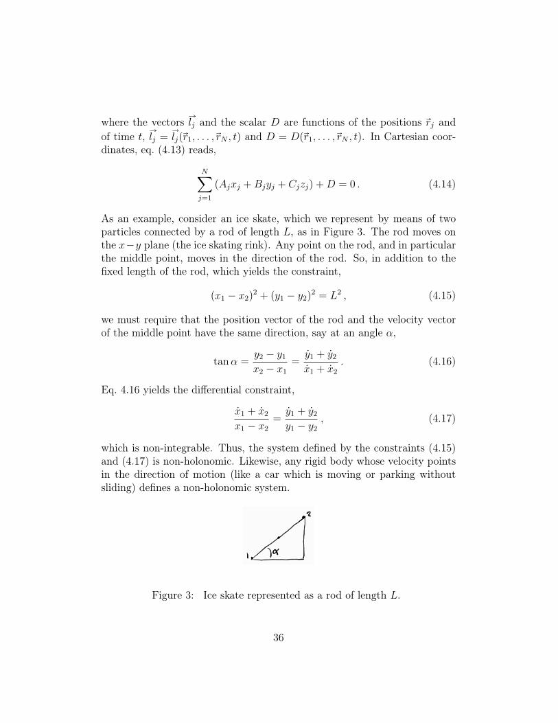
As an example, consider an ice skate, which we represent by means of twoparticles connected by a rod of length L, as in Figure 3. The rod moves onthe x−y plane (the ice skating rink). Any point on the rod, and in particularthe middle point, moves in the direction of the rod. So, in addition to thefixed length of the rod, which yields the constraint,
(x1 − x2)2 + (y1 − y2)2 = L2 , (4.15)
we must require that the position vector of the rod and the velocity vectorof the middle point have the same direction, say at an angle α,
tanα =y2 − y1
x2 − x1
=y1 + y2
x1 + x2
. (4.16)
Eq. 4.16 yields the differential constraint,
x1 + x2
x1 − x2
=y1 + y2
y1 − y2
, (4.17)
which is non-integrable. Thus, the system defined by the constraints (4.15)and (4.17) is non-holonomic. Likewise, any rigid body whose velocity pointsin the direction of motion (like a car which is moving or parking withoutsliding) defines a non-holonomic system.
Figure 3: Ice skate represented as a rod of length L.
36
4.2 Possible and virtual displacements
Let us take a system of N particles Pj, with j = 1, . . . , N , subject to dmanifestly holonomic constraints,
fi(r1, . . . , rN , t) = 0 , i = 1, . . . , d , (4.18)
and to g linear differential constraints,
N∑j=1
lkj · rj +Dk = 0 , k = 1, . . . , g . (4.19)
By taking the total time derivative of the manifestly holonomic contraints,like in Eq. 4.8,
N∑j=1
∇jfi · rj +∂fi∂t
= 0 , i = 1, . . . , d , (4.20)
we replace them by linear differential constraints as well. We see that theconstraints of Eqs 4.19-4.20 limit the allowed velocities rj of the particles.The velocities rj which are allowed by the constraints Eqs 4.19-4.20 are calledpossible. At a given time t and positions rj of the particles Pj, there areinfinitely many sets of possible velocities, since we have not yet consideredthe other forces (not responsible for constraints) which are acting on thesystem. Once we do so, only one set of possible particle velocities is actuallyrealised in the motion of the system.
Multiplying eqs. (4.19) and (4.20) by the time interval dt,
N∑j=1
∇jfi · drj +∂fi∂tdt = 0 , i = 1, . . . , d ,
N∑j=1
lkj · drj +Dkdt = 0 , k = 1, . . . , g , (4.21)
we write the linear differential constraints in terms of the possible displace-ments, drj = rjdt.
For two possible displacements,
drj = rjdt , dr′j = r′jdt , (4.22)
37
satisfying the constraints of Eq. 4.21, the difference
δrj = drj − dr′j , (4.23)
fulfils the constraintsN∑j=1
∇jfi · δrj = 0 , i = 1, . . . , d ,
N∑j=1
lkj · δrj = 0 , k = 1, . . . , g , (4.24)
In Cartesian coordinates the above can be written explicitly as:
N∑j=1
(∂fi∂xj
δxj +∂fi∂yj
δyj +∂fi∂zj
δzj
)= 0 , i = 1, . . . , d ,
N∑j=1
(Akjxj +Bkjyj + Ckjzj) = 0 , k = 1, . . . , g . (4.25)
The displacements of Eq. 4.23 are called virtual. We can think of virtualdisplacements as the ones which take a possible configuration of the systemat a time t to another one infinitely close to it, at the same time t. Forstationary constraints, which have a vanishing time derivative, the set ofvirtual displacements coincides with the one of the possible displacements.
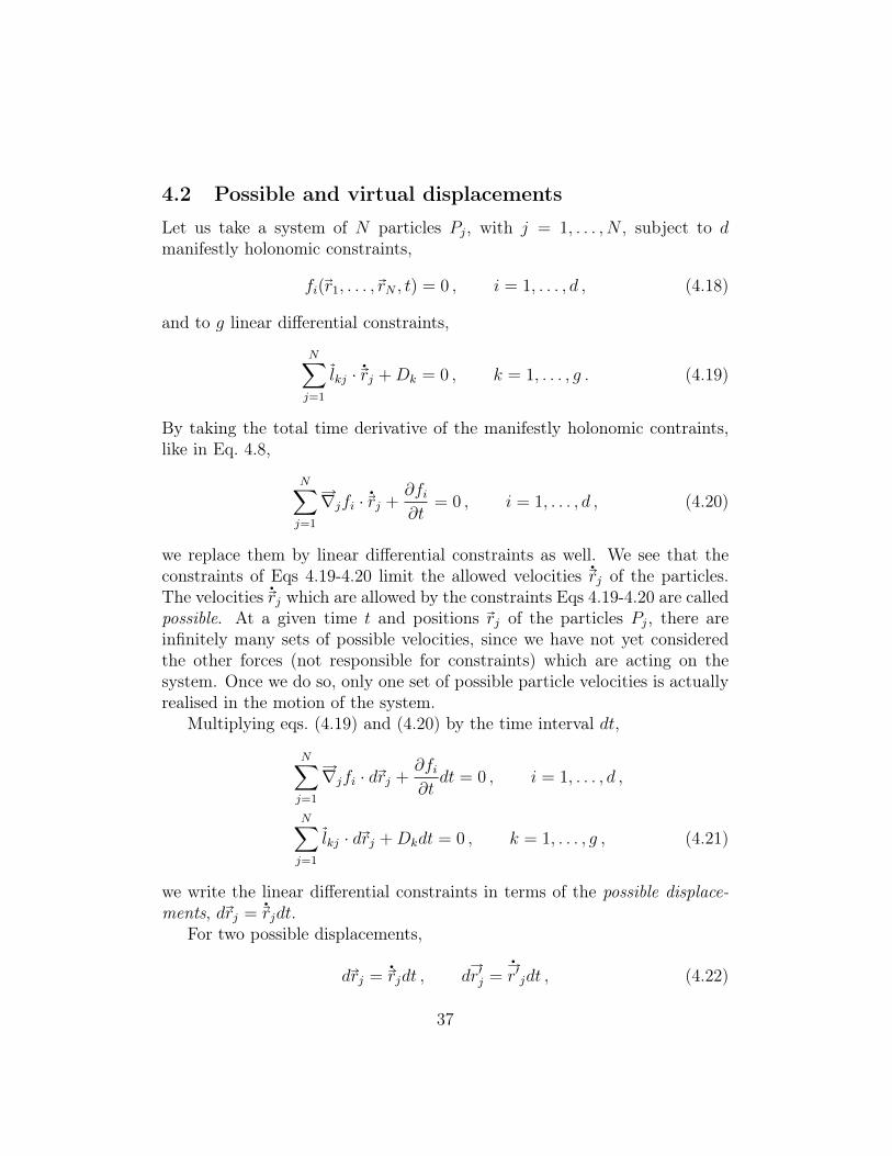
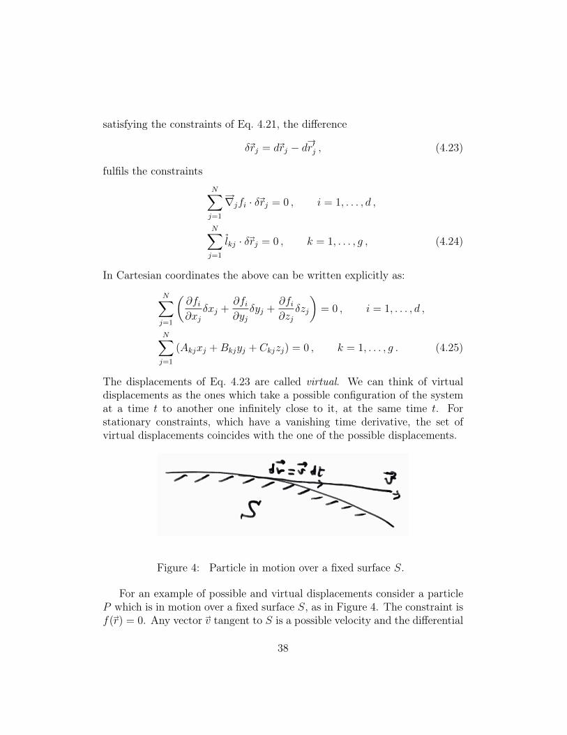
Figure 4: Particle in motion over a fixed surface S.
For an example of possible and virtual displacements consider a particleP which is in motion over a fixed surface S, as in Figure 4. The constraint isf(r) = 0. Any vector v tangent to S is a possible velocity and the differential
38
elements dr = v dt are possible displacements. The difference δr = dr−dr′ oftwo tangent vectors is also a tangent vector. In this case, the sets of virtualand possible displacements coincide, as we expect since the constraint isstationary.
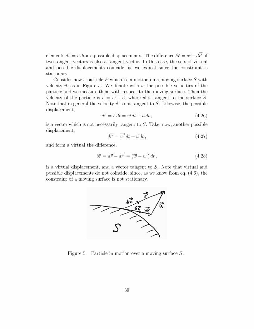
Consider now a particle P which is in motion on a moving surface S withvelocity u, as in Figure 5. We denote with w the possible velocities of theparticle and we measure them with respect to the moving surface. Then thevelocity of the particle is v = w + u, where w is tangent to the surface S.Note that in general the velocity v is not tangent to S. Likewise, the possibledisplacement,
dr = v dt = w dt+ u dt , (4.26)
is a vector which is not necessarily tangent to S. Take, now, another possibledisplacement,
dr′ = w′ dt+ u dt , (4.27)
and form a virtual the difference,
δr = dr − dr′ = (w − w′) dt , (4.28)
is a virtual displacement, and a vector tangent to S. Note that virtual andpossible displacements do not coincide, since, as we know from eq. (4.6), theconstraint of a moving surface is not stationary.
Figure 5: Particle in motion over a moving surface S.
39
4.3 Smooth constraints
From eq. (4.25), we know that for a system of N particles Pj, with j =1, . . . , N , we have 3N virtual displacements constrained by d geometric con-straints (4.18) and g differential constraints (4.19). Thus there are 3N−d−gindependent virtual displacements. We can say that our system ofN particleshas 3N − d− g degrees of freedom. The constraints, imply some restrictionsin the acceleration of the particles. In fact, taking the total time derivativeof eq. (4.8) for d constraints, we obtain
N∑j=1
∇jfi · rj +N∑j=1
(d
dt∇jfi
)· rj +
d
dt
∂fi∂t
= 0 , i = 1, . . . , d ,
N∑j=1
lkj · rj +N∑j=1
dlkjdt· rj +
dDk
dt= 0 , k = 1, . . . , g . (4.29)
Let us imagine for a moment the system without constraints. On thesystem are applied forces,
Fj = Fj(ri, ri, t) , j = 1, . . . , N , (4.30)
which are known functions of the positions ri and the velocities ri of theparticles. Without constraints, the forces would induce accelerations:
Fj = mjrj j = 1, . . . , N , (4.31)
where mj are the masses of the particles. However, if the system is con-strained, the accelerations rj are also due to additional forces Rj, calledreaction forces, which are responsible for the constraints. The accelerationsconsistent with Eq. 4.29 should satisfy:
mjrj = Fj +Rj , j = 1, . . . , N . (4.32)
The general problem of the dynamics of a constrained system is as fol-lows: given the forces Fj and the initial positions r0,i and velocities r0,i ofthe particles, we need to determine the trajectories of the particles and thereaction forces Rj of the constraints:
ri(t) , Rj , j = 1, . . . , N , (4.33)
40
Often ( if d+ g < 3N), the known equations of motion and constraints
mjrj = Fj +Rj , j = 1, . . . , N ,
fi(rj, t) = 0 , i = 1, . . . , d , (4.34)N∑j=1
lkj · rj +Dk = 0 , k = 1, . . . , g .
do not suffice to determine all unknowns, leaving n = 3N − d− g degrees offreedom undetermined. In order to determine the motion of the system, weneed additional n = 3N − d − g independent relations among the variables(4.33). We will find the necessary additional equations by examining theproperties of the constraints and making an assumption for the reactionforces which generate them.
There is a large class of constraints, called smooth, for which the work ofthe reaction forces vanishes over the virtual displacements,
N∑j=1
Rj · δrj = 0 , (4.35)
which in Cartesian coordinates is
N∑j=1
(Rj,xδxj +Rj,yδyj +Rj,zδzj) = 0 . (4.36)
Consider the following examples:
Example 4.1. Consider a particle P which moves on a fixed smooth surfaceS, as in Figure 6. As we have seen, the virtual and possible displacementscoincide in that case; they are vectors tangent to S. Because S is smooth(there are no frictions), the reaction force R is orthogonal to S. Then R·dr =0 and R · δr = 0. Therefore, the constraint is smooth.
Example 4.2. We now consider a pendulum, for which we have cast theconstraint, Eq. 4.11, in the differential form r · r = 0. Because the virtualand possible displacements coincide, it is also true that r · δr = 0, where thedirection of the string r identifies also the direction of the reaction force R.Thus, we have that R · δr = 0 and the constraint is therefore smooth.
41
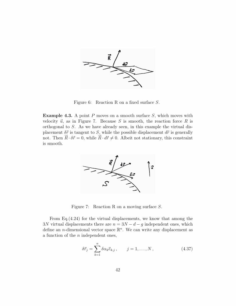
Figure 6: Reaction R on a fixed surface S.
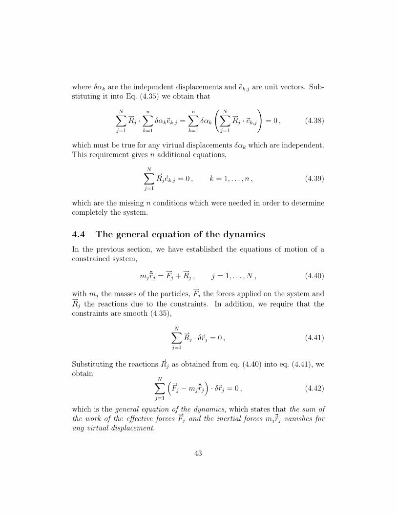
Example 4.3. A point P moves on a smooth surface S, which moves withvelocity u, as in Figure 7. Because S is smooth, the reaction force R isorthogonal to S. As we have already seen, in this example the virtual dis-placement δr is tangent to S, while the possible displacement dr is generallynot. Then R · δr = 0, while R · dr 6= 0. Albeit not stationary, this constraintis smooth.
Figure 7: Reaction R on a moving surface S.
From Eq.(4.24) for the virtual displacements, we know that among the3N virtual displacements there are n = 3N − d− g independent ones, whichdefine an n-dimensional vector space Rn. We can write any displacement asa function of the n independent ones,
δrj =n∑k=1
δαkek,j , j = 1, . . . , N , (4.37)
42
where δαk are the independent displacements and ek,j are unit vectors. Sub-stituting it into Eq. (4.35) we obtain that
N∑j=1
Rj ·n∑k=1
δαkek,j =n∑k=1
δαk
(N∑j=1
Rj · ek,j
)= 0 , (4.38)
which must be true for any virtual displacements δαk which are independent.This requirement gives n additional equations,
N∑j=1
Rjek,j = 0 , k = 1, . . . , n , (4.39)
which are the missing n conditions which were needed in order to determinecompletely the system.
4.4 The general equation of the dynamics
In the previous section, we have established the equations of motion of aconstrained system,
mjrj = Fj +Rj , j = 1, . . . , N , (4.40)
with mj the masses of the particles, Fj the forces applied on the system andRj the reactions due to the constraints. In addition, we require that theconstraints are smooth (4.35),
N∑j=1
Rj · δrj = 0 , (4.41)
Substituting the reactions Rj as obtained from eq. (4.40) into eq. (4.41), weobtain
N∑j=1
(Fj −mjrj
)· δrj = 0 , (4.42)
which is the general equation of the dynamics, which states that the sum ofthe work of the effective forces Fj and the inertial forces mjrj vanishes forany virtual displacement.
43
4.5 Independent generalised coordinates
In what follows, we will limit ourselves to a system of N particles, with dconstraints,
fi(rj, t) = 0 , i = 1, . . . , d . (4.43)
written in a manifestly holonomic form.We know from eq.(4.24) that among the 3N virtual displacements there
are n = 3N − d independent ones. Thus we can express the d equations(4.43) as functions of n independent coordinates, qi with i = 1, . . . , n, and ofthe time t. Also the positions of the particles can be taken as functions ofthe n independent coordinates,
rj = rj(q1(t), . . . , qn(t), t) , j = 1, . . . , N , (4.44)
In the specific case of stationary contraints (4.3), the positions of the particlesrj do not depend explicitly on the time t but only through qi(t).
The essential information about the degrees of freedom being reducedfrom 3N to n is encoded into the n independent coordinates of eq. (4.44),thus if we substitute eq. (4.44) into eq. (4.43), these become identities. Then independent coordinates qi are called independent generalised coordinates.Consider the following examples:
Example 4.4. A pendulum is moving on the x− z plane and it is attachedto a string of length R. the motion of the pendulum spans an angle φ:the pendulum has only one degree of freedom. The stationary holonomicconstraint is given by the equation,
x2 + z2 −R2 = 0 . (4.45)
If we take φ as the independent coordinate, then Eqs. 4.44 become
x = R cosφ ,
z = R sinφ . (4.46)
If we substitute the Eqs. 4.46 into Eq. 4.45, we obtain the identity,
cos2 φ+ sin2 φ− 1 = 0 . (4.47)
Example 4.5. A particle is constrained to move on a sphere of radius R: itcan move with two degrees of freedom. As independent coordinates, we can
44
take the longitude φ and the latitude θ. The holonomic stationary constraintis given by the equation,
x2 + y2 + z2 −R2 = 0 . (4.48)
In terms of the φ and θ angles, Eqs. 4.44 become
x = R cosφ cos θ ,
y = R sinφ cos θ , (4.49)z = R sin θ .
If we substitute the Eqs. (4.50) into the constraint of Eq. (4.48), we obtainthe identity,
(cos2 φ+ sin2 φ) cos2 θ + sin2 θ − 1 = 0 . (4.50)
4.6 Euler-Lagrange equations for systems with smoothconstraints and potential forces
We may now express the 3N virtual displacements as a function of the n =3N − d independent coordinates Eq. 4.44,
δrj =n∑i=1
∂rj∂qi
δqi , j = 1, . . . , N , (4.51)
and substitute it into the general equation of the dynamics (Eq. 4.42),
n∑i=1
N∑j=1
(Fj −mjrj
)· ∂rj∂qi
δqi = 0 , (4.52)
where we have inverted the order of the sums. Because the coordinates qi areindependent, so are their virtual displacements δqi. Thus, their coefficientsmust identically vanish, yielding:
N∑j=1
(Fj −mjrj
)· ∂rj∂qi
= 0 , i = 1, . . . , n . (4.53)
The first term of Eq. 4.53,N∑j=1
Fj ·∂rj∂qi≡ Qi , i = 1, . . . , n . (4.54)
45
is called the generalised force. The generalised force has the dimension ofa force only if the independent coordinates have the dimension of a length.Now let us analyse the second term of Eqs. 4.53,
N∑j=1
mjrj ·∂rj∂qi
, i = 1, . . . , n , (4.55)
which we rewrite as
N∑j=1
mjdrjdt· ∂rj∂qi
=d
dt
(N∑j=1
mjrj ·∂rj∂qi
)−
N∑j=1
mjrj ·d
dt
∂rj∂qi
, (4.56)
Next, we derive a couple of useful identities. We start from the velocities interms of independent coordinates,
rj =n∑i=1
∂rj∂qi
qi +∂rj∂t
, (4.57)
from which we immediately obtain that
∂rj∂qi
=∂rj∂qi
. (4.58)
Then we derive eq. (4.57) with respect to the independent coordinates,
∂rj∂qi
=n∑k=1
∂2rj∂qi∂qk
qk +∂2rj∂qi∂t
=d
dt
∂rj∂qi
. (4.59)
We substitute the identities (4.58) and (4.59) into eq. (4.56) and we obtain,
N∑j=1
mjrj ·∂rj∂qi
=d
dt
(N∑j=1
mjrj ·∂rj∂qi
)−
N∑j=1
mjrj ·∂rj∂qi
. (4.60)
Considering that the kinetic energy of the holonomic system of N particlesis,
T =1
2
N∑j=1
mj r2j , (4.61)
46
we can rewrite eq. (4.60) as
N∑j=1
mjrj ·∂rj∂qi
=d
dt
∂T
∂qi− ∂T
∂qi, i = 1, . . . , n . (4.62)
Substituting it into eq. (4.53) and remembering the definition of generalisedforce (4.54), we obtain:
d
dt
∂T
∂qi− ∂T
∂qi= Qi , i = 1, . . . , n . (4.63)
These equations form a system of n second order differential equations in nunknown variables qi. Therefore, the motion of the holonomic system withn degrees of freedom is determined fully if the values of qi and qi are givenat an initial time t0.
Note that the reaction forces Rj do not appear explicitly in Eqs. 4.63.They can be obtained by solving Eqs. 4.63 first, and then using Eq. 4.40.
Now, let us suppose that some forces can be derived from a potentialenergy U = U(qi, t),
Fj = −∂U∂rj
, (4.64)
such that the generalised forces become
Qi =N∑j=1
Fj ·∂rj∂qi
= −N∑j=1
∂U
∂rj· ∂rj∂qi
= −∂U∂qi
, i = 1, . . . , n , (4.65)
and that in addition there are non-potential generalised forces,
Qi = Qi(qk, qk, t) . (4.66)
Eqs. 4.63) become
d
dt
∂T
∂qi− ∂T
∂qi= −∂U
∂qi+ Qi , i = 1, . . . , n . (4.67)
Recalling the defintion of the Lagrangian,
L = T − U , (4.68)
47
we can cast Eq. 4.67 in the form:
d
dt
∂L∂qi− ∂L∂qi
= Qi , i = 1, . . . , n . (4.69)
In the absence of non-potential forces equations 4.67) give the Euler-Lagrangeequations:
d
dt
∂L
∂qi− ∂L
∂qi= 0 , i = 1, . . . , n . (4.70)
We have therefore proved that Hamilton’s principle of least action, whichyields the same Euler-Lagrange equations, should also hold for constrainedsystems with smooth holonomic constraints and potential forces.
48
5 Application of Euler-Lagrange equations: Sim-ple pendulum
We have seen that we can obtain the equations of motion for a system withholonomic constraints from a Lagrangian L by requiring that the action inte-gral is ninimum. This gives rise to Euler-Lagrange equations (the equationsof motion):
d
dt
∂L∂qi− ∂L∂qi
= 0 (5.1)
In the above, all generalised coordinates qi are independent, and we havefirst used the holonomic constraints to eliminate additional variables whichare not independent.
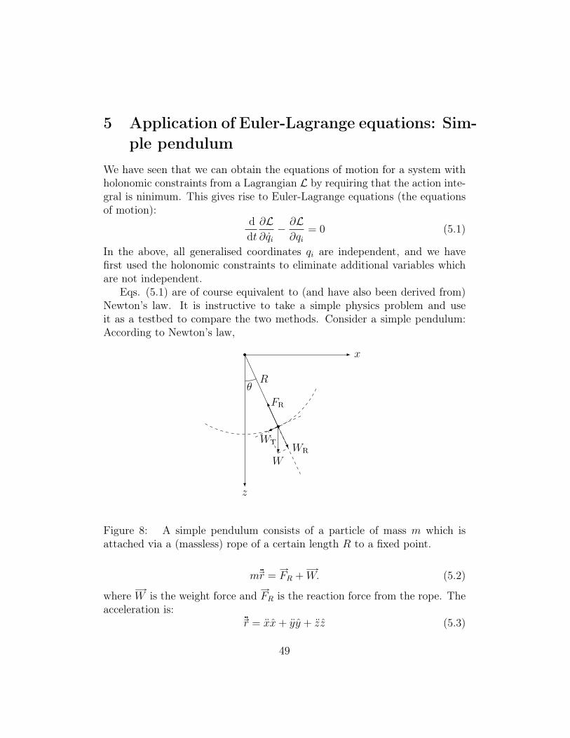
Eqs. (5.1) are of course equivalent to (and have also been derived from)Newton’s law. It is instructive to take a simple physics problem and useit as a testbed to compare the two methods. Consider a simple pendulum:According to Newton’s law,
x
z
FR
θ
W
WTWR
R
Figure 8: A simple pendulum consists of a particle of mass m which isattached via a (massless) rope of a certain length R to a fixed point.
mr = FR +W. (5.2)
where W is the weight force and FR is the reaction force from the rope. Theacceleration is:
r = xx+ yy + zz (5.3)
49
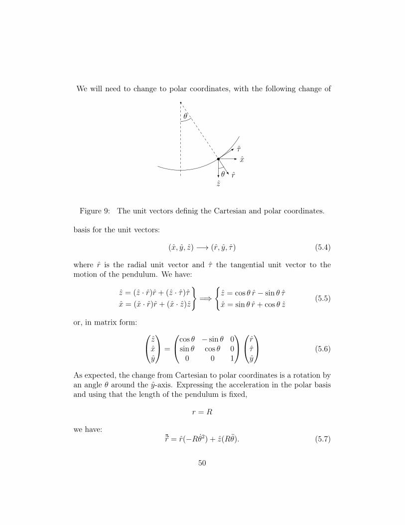
We will need to change to polar coordinates, with the following change of
θ
rz
x
τ
θ
Figure 9: The unit vectors definig the Cartesian and polar coordinates.
basis for the unit vectors:
(x, y, z) −→ (r, y, τ) (5.4)
where r is the radial unit vector and τ the tangential unit vector to themotion of the pendulum. We have:
z = (z · r)r + (z · τ)τ
x = (x · r)r + (x · z)z
=⇒
z = cos θ r − sin θ τ
x = sin θ r + cos θ z(5.5)
or, in matrix form: zxy
=
cos θ − sin θ 0sin θ cos θ 0
0 0 1
rτy
(5.6)
As expected, the change from Cartesian to polar coordinates is a rotation byan angle θ around the y-axis. Expressing the acceleration in the polar basisand using that the length of the pendulum is fixed,
r = R
we have:r = r(−Rθ2) + z(Rθ). (5.7)
50
The force acting on the pendulum is decomposed as:
F = W + FR = −(mg sin θ)z + (mg cos θ − FR)r.
Newton’s law gives then two equations: The equation of motion determiningthe evolution of the angle θ:
mRθ = −mg sin θ ; θ +g
Rsin θ = 0 (5.8)
and an equation which determines the reaction force:
−mRθ2 = mg cos θ − FR ; FR = m(Rθ2 + g cos θ) (5.9)
Let us now use the Euler-Lagrange method. The Lagrangian is
L = T − V =1
2mr2 −mg(z0 − z).
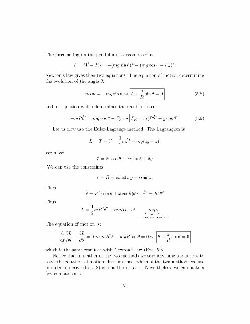
We have:r = zr cos θ + xr sin θ + yy
We can use the constraints
r = R = const., y = const..
Then,r = R(z sin θ + x cos θ)θ ; r2 = R2θ2
Thus,
L =1
2mR2θ2 +mgR cos θ −mgz0︸ ︷︷ ︸
unimportant constant
The equation of motion is:
d
dt
∂L
∂θ− ∂L
∂θ= 0 ; mR2θ +mgR sin θ = 0 ; θ +
g
Rsin θ = 0
which is the same result as with Newton’s law (Eqs. 5.8).Notice that in neither of the two methods we said anything about how to
solve the equation of motion. In this sence, which of the two methods we usein order to derive (Eq 5.8) is a matter of taste. Nevertheless, we can make afew comparisons:
51
x
z
r cos θ
r sin θ
r
θ
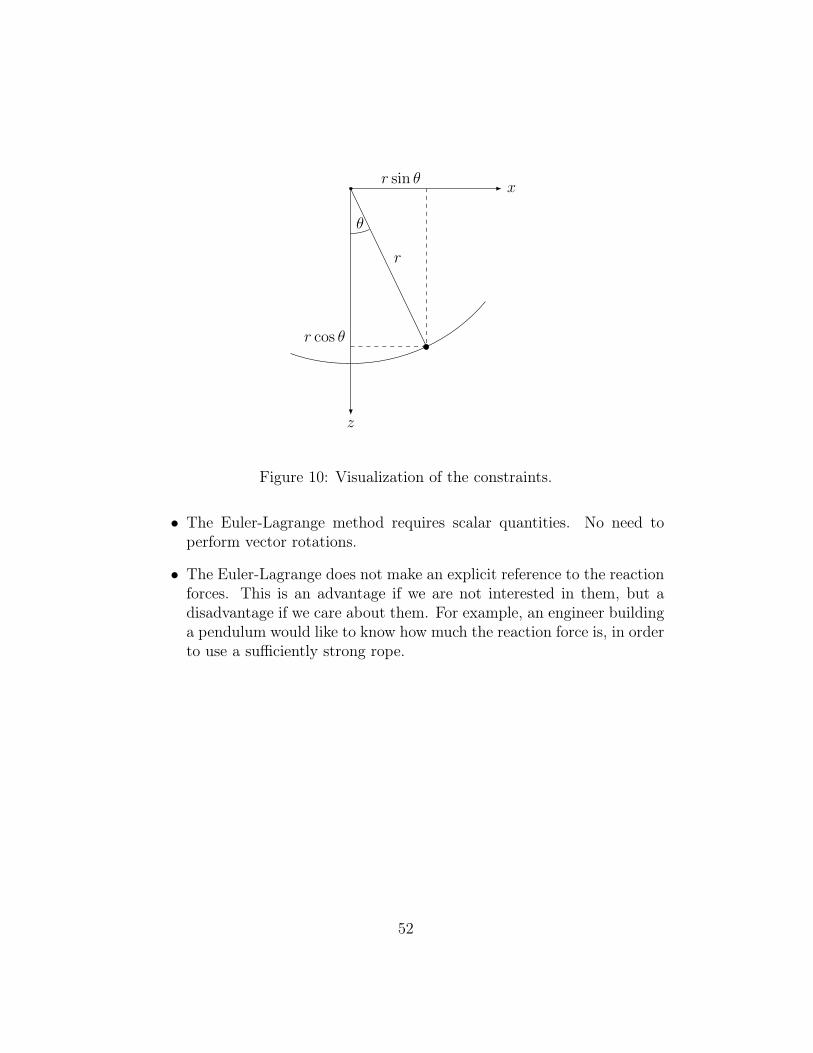
Figure 10: Visualization of the constraints.
• The Euler-Lagrange method requires scalar quantities. No need toperform vector rotations.
• The Euler-Lagrange does not make an explicit reference to the reactionforces. This is an advantage if we are not interested in them, but adisadvantage if we care about them. For example, an engineer buildinga pendulum would like to know how much the reaction force is, in orderto use a sufficiently strong rope.
52
6 Minimization with Lagrange multipliersThe mathematical problem that we are facing in classical mechanics is oneof minimization of a functional (the action). This problem becomes morecomplicated due to contstraints which make the variables of the functional(generalized coordinates) not independent. We have seen that for simple con-straints (holonomic) it may be possible to eliminate the dependent variables.When this is not possible, we may consider the more sophisticated techniqueof Lagrange multipliers. We will recall the salient features of this method forthe minimization of functions with constraints first and then we will see howto apply it for functionals and the action specifically.
6.1 Minimization of a multivariate function with La-grange multipliers
Consider a functionu = f(x1, . . . , xN)
where x1, . . . , xN are all independent variables. We are interested in findingthe extrema (minima or maxima) of the function. These are given by thecondition that the total differential of the function vanishes:
du = 0⇒N∑i=1
∂f
∂xidxi = 0.
Since we have taken the variables xi to be independent, the coefficients ofdxi must all vanish. Thus, we have that an extremum occurs if
∂f
∂xi= 0 ∀i = 1, . . . , N.
Let us now assume that the variables xi are not all independent due to, forexample, a constraint:
φ(x1, . . . , xN) = 0.
The extrema of the function are given in this case too by the condition
du = 0,
53
but unlike earlier one of the variables, let’s say xN , is not independent anymore. A straightforward way to find the minimum would be to solve theconstraint
φ(x1, . . . , xN) = 0 ; xN = xN(x1, . . . , xN−1)
and eliminate this variable from the function:
u = f(x1, . . . , xN(x1, . . . , xN−1)) = g(x1, . . . , xN−1)
Then, we can minimize g(x1, . . . , xN−1) as before, since the remaining vari-ables are all independent. However, there is an alternative way where we donot need to solve the constraint explicitly. We start from
du = 0 ;
N−1∑i=1
(∂f
∂xi+
∂f
∂xN
∂xN∂xi
)dxi = 0
;
N−1∑i=1
∂f
∂xidxi +
∂f
∂xN
N−1∑i=1
∂xN∂xi
dxi = 0. (6.1)
The sum in the last term is:N−1∑i=1
∂xN∂xi
dxi = dxN .
We therefore find again the same condition
du = 0 ;∂f
∂xidxi + · · ·+ ∂f
∂xN−1
dxN−1 +∂f
∂xNdxN = 0, (6.2)
although now the dxi’s are not all independent and we cannot demand thattheir coefficients vanish independently. Consider now the constraint:
φ(x1, . . . , xN) = 0 ; dφ(x1, . . . , xN) = 0
⇒ ∂φ
∂x1
dx1 + · · ·+ ∂φ
∂xNdxN = 0 (6.3)
We can multiply (6.3) with a constant λ, the so called Lagrange multiplier,and subtract it from (6.2):
N∑i=1
[∂f
∂xi− λ ∂f
∂xi
]dxi = 0
54
It can be proven (Analysis course) that we can use the extra parameter λ inorder to make all terms in the brackets to vanish,
∂f
∂xi− λ ∂φ
∂xi= 0 i = 1, . . . , N.
Solving the system of equations above will determine the minimum.Therefore, the procedure to find the extremum in the presence of a con-
straint is identical to the one without contraints, replacing the original func-tion
f(x1, . . . , xN)
with a function which includes the constraint
fλ(x1, . . . , xN) ≡ f(x1, . . . , xN)− λφ(x1, . . . , xN).
Let’s see how this works in a couple of examples.
Example 6.1. Find the minimum distance of a straight line from the origin.We will solve this problem in two ways:
1. Eliminating dependent variables.The square of the distance of a point (x, y) from the origin is:
f(x, y) ≡ d(x, y)2 = x2 + y2.
The constraint demands that the point belongs to a line
y = ax+ b a, b ∈ R.
Eliminating the y-variable, we have:
f(x, y) = f(x, y(x)) = x2 + (ax+ b)2 ≡ g(x).
We now have one independent variable x. We can minimize, by de-manding:
∂g(x)
∂x= 0 ; 2x+ 2a(ax+ b) = 0⇒ x =
−ab1 + a2
Theny = a
(−ab
1 + a2
)+ b =
b
1 + a2.
The mininum distance of the line to the origin is therefore at the point
(x, y) =
(−ab
1 + a2,
b
1 + a2
)
55
2. Using Lagrange multipliers.We first define the function
fλ(x, y) = x2 + y2 − λ(y − ax− b)
which contains the square of the distance of the pont (x,y) as well asa Lagrange multiplier with the constraint that the point must belongto a line y− ax− b = 0. We require that the partial derivatives of thisfunction with respect to all variables must vanish:
∂
∂xfλ(x, y) = 0
∂
∂yfλ(x, y) = 0
⇒ 2x+ λa = 0
2y − λ = 0
⇒ x = −λ2a
y =λ
2
We can now use the constraint:
y − ax− b = 0⇒ λ
2(1 + a2) = b⇒ λ =
2b
1 + a2.
Thus the minimum is at
(x, y) =
(−a
1 + a2b,
b
1 + a2
)as expected.
You may wonder what is the advantage of Lagrange multipliers sincein our first example it was trivial to solve the problem by eliminating thedependent variable. However, it occurs in other problems to be easier (or theonly possibility) to solve for a Lagrange multiplier instead. We demonstratethis in the following more complicated example.
Example 6.2. Find the minimum and maximum distance from the originon an ellipse
x2
a2+y2
b2= 1.
We introduce a Lagrange mutiplier for the constraint and minimize the func-tion
fλ(x, y) = x2 + y2 − λ(x2
a2+y2
b2− 1
)
56
by demanding that
∂fλ∂x
= 0 ; x
(1− λ
a2
)= 0
∂fλ∂y
= 0 ; y
(1− λ
b2
)= 0
andx2
a2+y2
b2= 1.
The solutions of the three equation are:
x = 0, λ = b2, y = ±bor
y = 0, λ = a2, x = ±a
The extrema are then
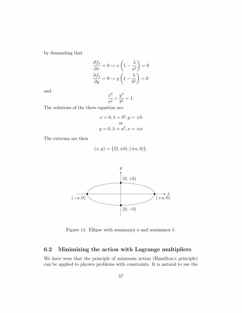
(x, y) = (0,±b), (±a, 0).
x
y
(+a, 0)(−a, 0)
(0,+b)
(0,−b)
Figure 11: Ellipse with semimajor a and semiminor b.
6.2 Minimizing the action with Lagrange multipliers
We have seen that the principle of minimum action (Hamilton’s principle)can be applied to physics problems with constraints. It is natural to use the
57
method of Lagrange multipliers in order to impose these constraints. We canachieve this as follows. Consider a system with qi independent coordinatesdescribed by the action
S =
∫dt L[qi, qi].
Minimizing the action gives
δS = 0 ;
∫dt∑i
δqi
[d
dt
∂L
∂qi− ∂L
∂qi
]= 0.
Since δqi’s are all independent of each other the coefficients must vanish,yielding the familiar Euler-Lagrange equations
d
dt
∂L
∂qi− ∂L
∂qi= 0.
In the presence of a constraint
f(qi, qi) = 0
the δqi’s are not independent independent anymore. From the constraint, wededuce that the following integral vanishes∫
dt λf(qi, qi) = 0
and thusδSλ = 0 with Sλ =
∫dt Lλ(qi, qi)
andLλ(qi, qi) = L(qi, qi)︸ ︷︷ ︸
originalLagrangian
− λxLagrangemultiplier
f(qi, qi)︸ ︷︷ ︸constraint
gives us
δSλ = 0 ;
∫dt∑i
δqi
[d
dt
∂Lλ∂qi− ∂Lλ
∂qi
]= 0.
The presence of the λ parameter allows us to take all the coefficients of δqito vanish
d
dt
∂Lλ∂qi− ∂L
∂qi= 0
besides the fact that the δqi’s are not independent.
58
Example 6.3. Let us solve the simple pendulum problem once again by usingLagrange multipliers this time. The Lagrangian with a Lagrange multiplierfor the constraint is
Lλ = T − V − λ(r− Rxconstant
)
withT =
1
2mr2 =
1
2mr2 +
1
2mr2θ2 and V = mgr cos θ.
The corresponding Euler-Lagrange equations are:
d
dt
∂Lλ∂r− ∂Lλ
∂r= 0 ; mr +mrθ2 +mg cos θ − λ = 0
d
dt
∂Lλ
∂θ− ∂Lλ
∂θ= 0 ; mr2θ +mg sin θ = 0.
Using in addition the constraint
r = R = const.
we have
θ +g
Lsin θ = 0 (6.4)
mg cos θ +mRθ2 = λ (6.5)
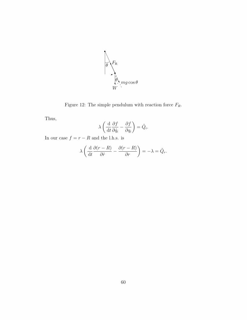
(6.4) is the equation of motion for the pendulum.(6.5) is very interesting. In the l.h.s. we recognize the reaction force FRthrough the rope. We see then that the Lagrange multiplier has some physicalmeaning in terms of the reaction force. This is not an accident. On one hand,we have:
d
dt
∂Lλ∂qi− ∂Lλ
∂qi= 0
;d
dt
∂L
∂qi− ∂L
∂qi= λ
(d
dt
∂f
∂qi− ∂f
∂qi
).
On the other hand, we have proven in general that
d
dt
∂L
∂qi− ∂L
∂qi= Qixgeneralized
forces
=N∑j=1
FR,jxnon-potential
forces
·∂rj∂qi
.
59
FRθ
θ
Wmg cos θ
Figure 12: The simple pendulum with reaction force FR.
Thus,
λ
(d
dt
∂f
∂qi− ∂f
∂qi
)= Qi.
In our case f = r −R and the l.h.s. is
λ
(d
dt
∂(r −R)
∂r− ∂(r −R)
∂r
)= −λ = Qr.
60
7 Conservation LawsObserving the time evolution of many physical systems, we often find thatcertain quantities remain invariant at all times. A classical example is the en-ergy of mechanical systems without friction. The Lagrangian formalism willallow us to gain a deeper understanding for the conservation of such quanti-ties. We will realize that conservation and symmetry are interconnected.
7.1 Conservation of energy
Let us take a look at systems with a Lagrangian
L[qi(t), qi(t), t] = L[qi(t), qi(t)].
The lack of explicit time dependence of the Lagrangian means that there isno special time. Whenever we let the system to evolve, it will be so in exactlythe same way irrespective of what is the starting time t0.
The total time derivative of the Lagrangian is:
d
dtL =
∑i
∂L∂qi
∂qi∂t
+∂L
∂qi
∂qi∂t
+∂L
∂t︸︷︷︸=0
=∑i
[∂L
∂qiqi +
∂L
∂qiqi
].
Let us now recall Euler-Lagrange equations
∂L
∂qi=
d
dt
∂L
∂qi.
Then we have:
dL
dt=∑i
[(d
dt
∂L
∂qi
)qi +
∂L
∂qiqi
]=
d
dt
∑i
∂L
∂qiqi
This implies thatd
dt
[∑i
∂L
∂qiqi − L
]= 0
61
and therefore ∑i
∂L
∂qiqi − L ≡ E = const. . (7.1)
We have found a conserved quantity, which we call energy. The reason forits invariance is the fact that the behaviour of the system does not change ifwe let it evolve at a different starting time.
We will now justify why the expression (7.1) is the familiar energy. Con-sider a particle with potential energy U(r). The Lagrangian is
L = T − U(r)
=1
2mr2 − U(r).
According to (7.1), the energy is
E =∂L
∂xx+
∂L
∂yy +
∂L
∂zz − L
= mx2 +my2 +mz2 − 1
2mr2 + U(r)
= mr2 − 1
2mr2 + U(r)
=1
2r2 + U(r) = T︸︷︷︸
kinetic
+ U︸︷︷︸potential
.
This is indeed the sum od the kinetic and potential energy.
7.2 Conservation of momentum
Let us now trace the origin of the conservation of momentum. We willfind that momentum is conserved for physical systems for which we canshift the position of all of their constituents without changing their physicalbehavior. For example, if a physical system can be studied in an experimentin Zürich but also in an independent experiment in New York, where the twoexperiments are anticipated to find the same results then the total momentumof the system is conserved. Formally, we assume that performing a translationfor the positions of all particles
ri → ri + ε
62
should leave the equations of motion invariant. Let us see how the Lagrangianchanges if ε is taken to be infinitesimal.
∆L = L[ri + ε, ri + ε, t]− L[ri, ri, t]
=N∑i=1
[∂L
∂ri,xεx +
∂L
∂ri,yεy +
∂L
∂ri,zεz
]
=N∑i=1
(∇iL · ε
).
The equations of motion are invariant by this displacement if the change inthe Lagrangian is zero:
∆L = 0 ; ε ·N∑i=1
∇iL = 0 .
The direction of ε is arbitrary. Choosing for example
ε = (1, 0, 0) or ε = (0, 1, 0) or ε = (0, 0, 1),
we obtainN∑i=1
∂L
∂xi= 0 and
N∑i=1
∂L
∂yi= 0 and
N∑i=1
∂L
∂xi= 0 (7.2)
where (xi, yi, zi) ≡ ri the position vector of the i-th particle. For the La-grangian of the form L = T − U Eq. (7.2) gives
∇iU = 0.
However, Fi = −∇U is the force acting on the i-th particle. Thus we concludethat
N∑i=1
Fi = 0 ,
where N is the number of particles in the system. In the special case of twoonly particles, N = 2, we have that
F1 = −F2
63
which is Newton’s “action and reaction” law.Let us now recall the Euler-Lagrange equations:
d
dt
∂L
∂xi=∂L
∂xid
dt
∂L
∂yi=∂L
∂yid
dt
∂L
∂zi=∂L
∂zi.
Then, we conclude that
d
dt
(∑i
∂L
∂xi
)=
d
dt
(∑i
∂L
∂yi
)=
d
dt
(∑i
∂L
∂zi
)= 0.
Therefore the quantities
Px ≡∑i
∂L
∂xi= const.
Py ≡∑i
∂L
∂yi= const.
Pz ≡∑i
∂L
∂zi= const..
are constant and the vector
P = (Px, Py, Pz)
is conserved. We can associate P with the total momentum of the system.
Exercise 7.1. For a Lagrangian
L =∑i
1
2mir
2
i − V (r1, . . . , rn) (7.3)
verify that∂L
∂xi= mixi,
∂L
∂yi= miyi,
∂L
∂zi= mizi. (7.4)
64
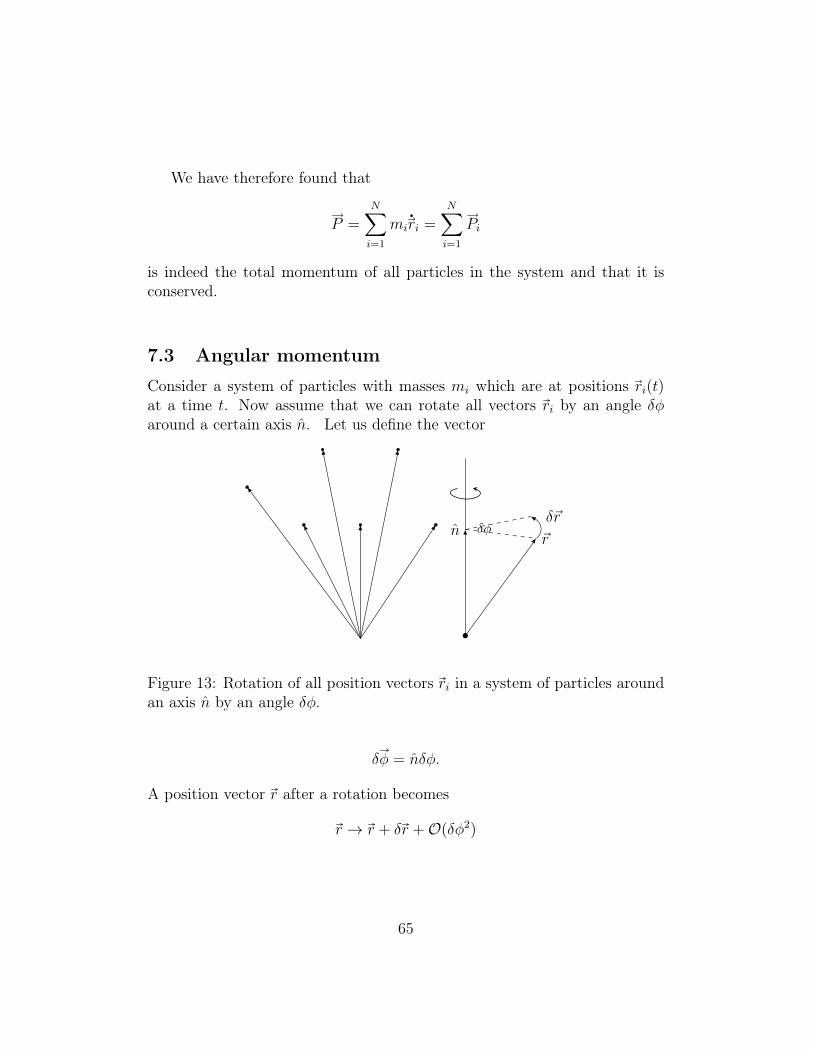
We have therefore found that
P =N∑i=1
miri =N∑i=1
Pi
is indeed the total momentum of all particles in the system and that it isconserved.
7.3 Angular momentum
Consider a system of particles with masses mi which are at positions ri(t)at a time t. Now assume that we can rotate all vectors ri by an angle δφaround a certain axis n. Let us define the vector
nδ~r
~rδφ
Figure 13: Rotation of all position vectors ri in a system of particles aroundan axis n by an angle δφ.
δφ = nδφ.
A position vector r after a rotation becomes
r → r + δr +O(δφ2)
65
with δr = δφ × r. For illustration, we can verify this for a rotation aroundthe z-axis:
r → r′ = R · r
=
cos δφ − sin δφ 0sin δφ cos δφ 0
0 0 1
xyz
≈
1 −δφ 0δφ 1 00 0 1
xyz
+O(δφ2)
=
xyz
+ δφ
0 −1 01 0 00 0 0
xyz
= r + δφ
−yx0
.
Consider
(n× r)i =∑j,k
εijknjrk n =
001
= εi3krk
Thus
(n× r)1 = ε132r2 = −1y = −y(n× r)2 = ε231r1 = +1x = x
(n× r)3 = ε133rk = 0
and
r → r′ = r + δr
= r + δφ× r +O(δφ2).
Now we can find what are the conserved quantities associated with rota-tion symmetry by repeating the same steps as for space translations in the
66
previous section. Under a rotation transformation the Lagrangian changesby
L→ L′ = L+ δL
with
δL ≡ L[r + δφ× r, r + δφ× r]− L[r, r]
=∑i
[∂L
∂xi(δri)x +
∂L
∂yi(δri)y +
∂L
∂zi(δri)z +
∂L
∂xi(δri)x +
∂L
∂yi(δri)y +
∂L
∂zi(δri)z
]=∑i
[Px,i(δri)x + Py,i(δri)y + Pz,i(δri)z + Px,i(δri)x + Py,i(δri)y + Pz,i(δri)z
]=
d
dtδφ ·
[∑i
ri × Pi
]
= δφ · d
dt
∑i
ri × Pi.
If this change of the Lagrangian is zero, then the rotation has no effect onthe physical system. This implies that
δL = 0 ; δφ · d
dt
∑i
ri × Pi = 0.
Since δφ is an arbitrary vector (we can choose the rotation axis at wish) wemust have:
d
dt
∑i
ri × Pi = 0⇒ M =∑i
ri × Pi = const. .
We have therefore found that the total angular momentum is conserved.
7.4 Summary of conservation laws & symmetry
We have realized that symmetry plays an important role in conservationlaws. In the following table we summarize out findings, for typical conservedquantities and their symmetry origin.
67
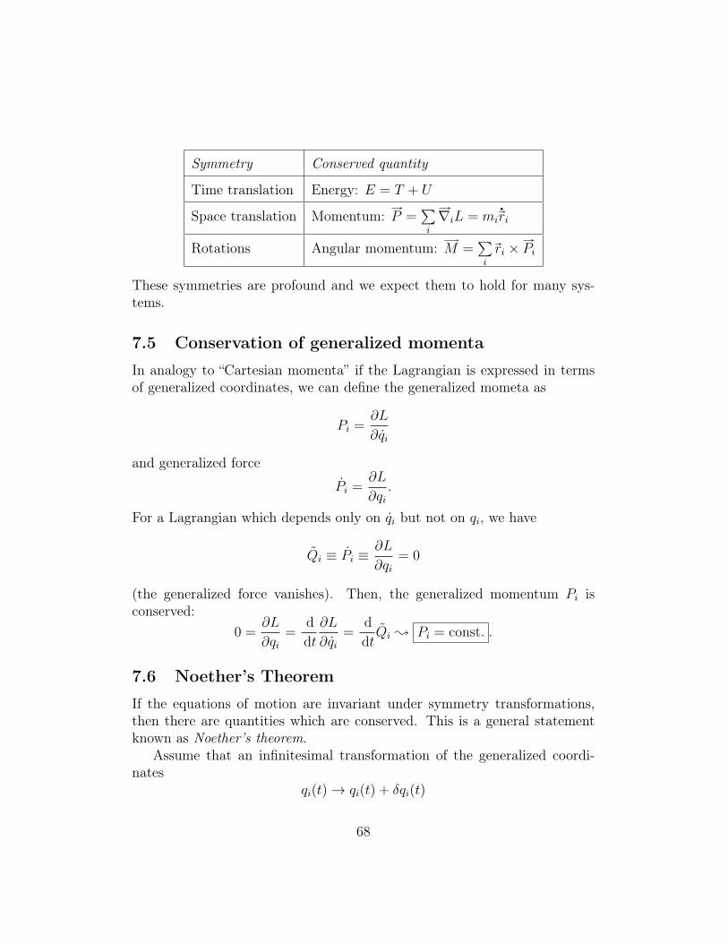
Symmetry Conserved quantity
Time translation Energy: E = T + U
Space translation Momentum: P =∑i
∇iL = miri
Rotations Angular momentum: M =∑i
ri × Pi
These symmetries are profound and we expect them to hold for many sys-tems.
7.5 Conservation of generalized momenta
In analogy to “Cartesian momenta” if the Lagrangian is expressed in termsof generalized coordinates, we can define the generalized mometa as
Pi =∂L
∂qi
and generalized force
Pi =∂L
∂qi.
For a Lagrangian which depends only on qi but not on qi, we have
Qi ≡ Pi ≡∂L
∂qi= 0
(the generalized force vanishes). Then, the generalized momentum Pi isconserved:
0 =∂L
∂qi=
d
dt
∂L
∂qi=
d
dtQi ; Pi = const. .
7.6 Noether’s Theorem
If the equations of motion are invariant under symmetry transformations,then there are quantities which are conserved. This is a general statementknown as Noether’s theorem.
Assume that an infinitesimal transformation of the generalized coordi-nates
qi(t)→ qi(t) + δqi(t)
68
is a symmetry transformation, i.e. it let’s the equations of motion invariant.The change that this transformation induces to the Lagrangian is
∆L =∑i
[∂L
∂qi∆qi +
∂L
∂qi∆qi
].
Using the Euler-Lagrange equations we substitute
∂L
∂qi=
d
dt
∂L
∂qi.
Then
∆L =∑i
[(d
dt
∂L
∂qi
)∆qi +
∂L
∂qi
d
dt(∆qi)
]=
d
dt
∑i
∂L
∂qi∆qi
⇒ ∆L =d
dt
∑i
∂L
∂qi∆qi .
If ∆L = 0, then the Lagrangian is invariant and the action is also invari-ant, leading to the same equations of motion. But we should be more careful!More generally, the action is invariant if the Lagrangian changes under thesymmetry transformation by a total time derivative:
∆L =dF
dt;
d
dt
∑i
∂L
∂qi∆qi =
dF
dt;
d
dt
(∑i
∂L
∂qi∆qi − F
)= 0.
Then we have that the quantity
J =∑i
∂L
∂qi∆qi − F
is a conserved quantity.
Example 7.1. Consider a particle in a homogeneous gravitational field:
L =1
2m(x2 + y2 + z2)−mgz.
69
Since the field along the z−axis, we expect that translations
z → z + a
to be a symmetry. With this transformation, the Lagrangian changes by
L→ L−mga⇒ ∆L = −mga = −a d
dt(mgt).
We have been able to cast the change as a total derivative. Then, accordingto Noether’s theorem,
∂L
∂z∆z = ∆L
∂L
∂z∆z = −a d
dt(mgt)
⇒ d
dt(mza) = −a d
dt(mgt)
⇒ d
dt(z + gt) = 0
⇒ z + gt = const. .
We have then found that there is a conserved quantity. We can verify thatthis is correct directly from the equation of motion:
d
dt
∂L
∂z− ∂L
∂z= 0⇒ mz +mg = 0
∫dt⇒ z + gt = const. .
For the other possible translations along the x and y directions induce nochange in the Lagrangian:
x→ x+ a⇒ ∆L = 0.
These are symmetry transformations. According to Noether’s theorem:
∂L
∂x∆x = const.⇒ mxa = const.⇒ x = const..
The equations of motion give
d
dt
∂L
∂x− ∂L
∂x= 0 ; mx = 0 ; x = const. .
and y → y + a; y = const., confirming the result of Noether’s theorem.
70
7.7 Noether’s theorem & time symmetries2
In the action integral,
S =
∫ tf
ti
dtL[qi(t), qi(t)] (7.5)
time is an integration variable, while the generalised coordinates qi and theircorresponding velocities qi are unintegrated parameters. In Eq. 7.6 we ex-amined a symmetry transformation which acts on the coordinates (integralparameters). However, as we have seen in Sec 7.1 a time symmetry (timetranslation), which affects the integration variable t of the action integral,leads to a conservation law. Our proof of Noether’s theorem in the previoussection does not cover this case. We will see here that Noether’s theorem canbe extended for symmetries of the integration variable as well. This proofwill be particularly useful in the future, when we study continuum systemsand fields. For convenience, in this Section we will use Einstein’s summationconvention: AiBi ≡
∑iAiBi.
Consider a symmetry transformation
t→ t′ = t′(t) = t+ δt
which leaves the action invariant:∫ tf
ti
dtL[qi(t), qi(t)] =
∫ t′f
t′i
dt′ L[q′i(t′), q′i(t
′)]
=
∫ tf
ti
dt
(dt′
dt
)L[q′(t′), q′i(t
′)]
=
∫ tf
ti
dt
[1 +
d
dtδt
]L[qi(t) + ∆q′i(t
′), qi(t′) + ∆qi(t
′)].
(7.6)
We have assumed that the coordinates also change by a certain amount whenwe perform this transformation:
qi(t)→ q′i(t′) = qi(t) + ∆q′i(t
′).
We can now write
L[q(t) + ∆q′i(t′), qi(t) + ∆q′i(t
′)] = L[qi(t), qi(t)] +∂L
∂qi∆q′i(t
′) +∂L
∂qi∆q′i(t
′).
2This section can be ommitted in a first reading. It is not part of an exam
71
Then, (7.6) gives that∫ tf
ti
dt
[L
dδt
dt+∂L
∂qi∆q′(t′) +
∂L
∂qi∆q′i(t
′) +∂L
∂tδt
]= 0. (7.7)
We decompose the change in the coordinates as follows:
∆q′i(t′) ≡ q′i(t
′)− qi(t)= q′i(t
′)− qi(t′)︸ ︷︷ ︸δ∗qi
+qi(t′)− qi(t)
= δ∗qi + qi(t) +d
dtqi(t)δt− qi(t)
= δ∗qi + qiδt
; ∆q′i(t′) = q′i(t
′)− qi(t′) + qiδt
where we separate the change due to changing the argument of the coordinatefunction from one time instant t to another t′ and an instantaneous changeof the function itself qi to q′i at the same time t′. Similarly,
∆q′i(t′) = q′i(t
′)− qi(t′) + qi(t′)− qi(t)
; ∆q′i =d
dt(δ∗qi) + qiδt.
Substituting into (7.7), we obtain:
0 =
∫ tf
ti
dt
[L
d
dtδt+
∂L
∂qi(δ∗qi + qδt) +
∂L
∂qi
(d
dtδ∗qi + qiδt
)]=
∫ tf
ti
dt
[L
d
dtδt+
(∂L
∂qiqi +
∂L
∂qiq
)δt
]+
(∂L
∂qiδ∗qi +
∂L
∂qi
d
dtδ∗qi
).
The term in the square bracket is:
d
dt[(δt)L[qi, qi]] = L
d
dt(δt) + δt
(∂L
∂qiqi +
∂L
∂qiqi
).
Thus
0 =
∫dt
[d
dt(Lδt) +
d
dt
∂L
∂qiδ∗qi +
∂L
∂qi
d
dtδ∗qi
]=
∫dt
d
dt
[Lδt+
∂L
∂qiδ∗qi
].
72
The above should hold for arbitrary boundaries. Thus we must have thatthe integrand must vanish:
⇒ Lδt+∂L
∂qiδ∗qi = const..
We can now write
δ∗qi = ∆qi − qiδt with ∆qi ≡ q′i(t′)− qi(t).
We then have (L− ∂L
∂qiqi
)δt+
∂L
∂qi∆qi = const. .
For the special case (but also very common) of ∆q = 0, we recover the resultof Section 7.1 that the energy is conserved:(
L− ∂L
∂qiqi
)= E = constant. (7.8)
7.8 Continuous Symmetry Transformations
As we have seen, symmetry plays an important role for the conservation ofphysical quantities. In this section, we will review some of the mathematicalproperties of continuous symmetry transformations.
Consider a set of generalized coordinates q1...qN
describing a system with a Lagrangian
L[qi(t), qi(t), t].
Assume that the system is symmetric under a symmetry transformation
qi → q′i = Tij(θa)qj where a = 1, . . . , N and i, j = 1, . . . ,M.
We take the parameters θa to be continuous. For example, if a system isdescribed by two Cartesian coordinates on a plane(
xy
)73
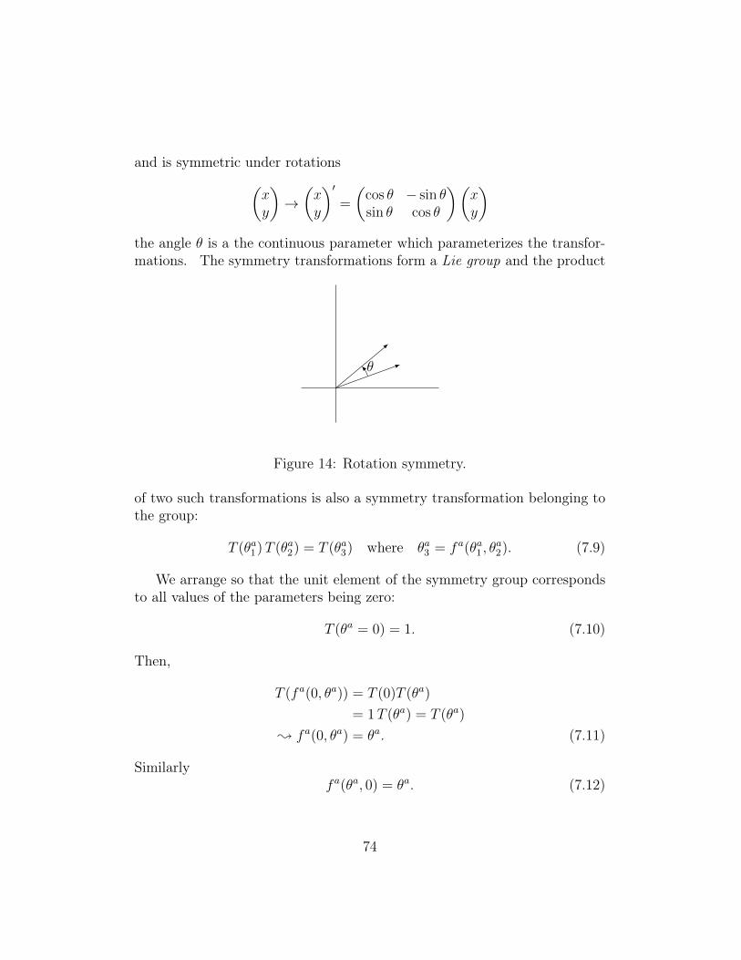
and is symmetric under rotations(xy
)→(xy
)′=
(cos θ − sin θsin θ cos θ
)(xy
)the angle θ is a the continuous parameter which parameterizes the transfor-mations. The symmetry transformations form a Lie group and the product
θ
Figure 14: Rotation symmetry.
of two such transformations is also a symmetry transformation belonging tothe group:
T (θa1)T (θa2) = T (θa3) where θa3 = fa(θa1 , θa2). (7.9)
We arrange so that the unit element of the symmetry group correspondsto all values of the parameters being zero:
T (θa = 0) = 1. (7.10)
Then,
T (fa(0, θa)) = T (0)T (θa)
= 1T (θa) = T (θa)
; fa(0, θa) = θa. (7.11)
Similarlyfa(θa, 0) = θa. (7.12)
74
Let us now perform a Taylor expansion around θa = 0:
θa1 = fa(θa1 ,7
0θa2 ) =fa(0, 0) +
∂fa
∂θb2θb1 +
@
@@@
∂fa
∂θb2θb2
+
*0
1
2
∂2fa
∂θb1∂θc1
θb1θc1 +
HHHH
HHH
1
2
∂2fa
∂θb2∂θc2
θb2θc2 +
HH
HHHH
∂2fa
∂θb1∂θc1
θb1θc2 + . . .
Impressing (7.11) and (7.12), we have
fa(θa1 , θa2) = θa1 + θa2 +
∑b,c
fabcθb1θc2 + . . .
For small θa parameters, we can expand:
T (θa) = 1 + iθata +1
2
∑b,c
θbθctbc + . . .
where 1, ta, tbc are matrices of the same dimensionality as T (θa). In addition
tbc = tcb (symmetric).
Making a Taylor expansion of (7.9), we have:(1 + iθa1ta +
1
2θb1θ
c2tbc
)(1 + iθd2td +
1
2θd1θ
e2tde
)=1 + i
(θa1 + θa2 + fabcθ
b1θc2 + . . .
)ta
+1
2
(θb1 + θb2 + . . .
)(θc1 + θc2 + . . . ) tbc + . . .
Matching the terms of the expansion, we have:
tbc = −tbtc − ifabcta.
From the symmetry of tbc = tcb:
tbtc + ifabcta = tctb + ifabcta
; tbtc − tctb = i(facb − fabc)ta
For reasons to become clear later, the matrices ta are called the generators ofthe symmetry transformations. We also define the commutator of two suchgenerators as:
[ta, tb] ≡ tatb − tbta.
75
The combinationsCabc ≡ facb − fabc
are called the structure constants and they are antisymmetric:
Cabc = −Ca
cb .
The equation[ta, tb] = iCa
bcta (7.13)
defines the Lie algebra of the group. Notice that
[ta, [tb, tc]] + [tb, [tc, ta]] + [tc, [ta, tb]] = 0. (7.14)
This is the so called Jacobi identity and it is satisfied by the generators. Thisgives an identity for the structure constants. Using the Lie algebra, we have:
[ta, ifdbctd] + [tb, if
dcatd] + [tc, if
dabtd] = 0
; CeadC
dbc + Ce
bdCdca + Ce
cdCdab = 0 .
Let us now define:tbac = iCc
ab.
Then the above equation becomes:
[ta, tb] = iCdabt
d, i.e.,
the structure constant furnish another representation of the Lie algebra. Wecall this the adjoint representation.
It is now time to justify why we call the ta matrices generators. Usingthe product rule of Eq. 7.9 an infinite amount of times, we can write for asymmetry transformation with parameters θa
T (θa) = limN→∞
T
(θa
N
)N(product rule)
= limN→∞
(1 + i
θa
Nta
)N= exp(iθata).
76
In other words, the generators ta, together with the product rule are sufficientto produce any ťťlarge” transformation from infinitesimal ones by means ofa simple exponentiation:
T (θa) = exp(iθata). (7.15)
Example 7.2. For rotations on a plane, we have:(x′
y′
)=
(cos θ − sin θsin θ cos θ
)︸ ︷︷ ︸
T (θ)
.
For a small θ angle:
T (θ) ≈(
1 00 1
)+ θ
(0 −11 0
)+O(θ2)
=
(1 00 1
)+ iθ
(0 i−i 0
)+O(θ2).
The generator is
t ≡(
0 i−i 0
)(we have only one). Notice that
t2 =
(0 i−i 0
)(0 i−i 0
)=
(1 00 1
)= 1.
Thus,
exp(iθt) =∞∑n=0
inθntn︸ ︷︷ ︸n!
=∞∑n=0
i2nθ2n(t2)n
(2n)!+∞∑n=0
i2n+1θ2n+1t2n+1
(2n+ 1)!
=∞∑n=0
(iθ)2n
(2n)!+ i
∞∑n=0
(iθ)2n+1
(2n+ 1)!.
77
But
eiθ = cos θ + i sin θ
=∞∑n=0
(iθ)2n
(2n)!+∞∑n=0
(iθ)2n+1
(2n+ 1)!.
Thus:
exp(iθt) = cos θ 1 + it sin θ
=
(cos θ 0
0 cos θ
)+
(0 −11 0
)sin θ
=
(cos θ − sin θsin θ cos θ
).
Exercise 7.2. Find the generators and structure constants for rotations in3 dimensions (SO(3) group).
78
8 Motion in one dimensionThe knowledge of conservation laws such as energy conservation can be help-ful for solving the equations of motion of a system and determining thetrajectories of its particles. We can demonstrate this in the simplest possibleexample, an one-particle system which is specified by one only generalizedcoordinate.
Let’s consider a Lagrangian of the form
L =1
2a(q)q2 − V (q)
with q a generalized coordinate. This Lagrangian does not depend explicitlyon time. Thus, the energy of the system is conserved:
E =∂L
∂qq − L =
1
2a(q)q2 + V (q) = const..
It now becomes easier to solve the equations of motion, without even havingwritten the Euler-Lagrange equation down. From energy conservation, wehave (
dq
dt
)2
=2(E − V (q))
a(q)
;
∫dt =
∫dq
a(q)12√
2(E − V (q))
⇒ t =
∫dq
√a(q)
2(E − V (q))+ const. .
For a particle moving in one dimension
q = x, a(q) = m, L =1
2mx2 − V (x)
we have
t− t0 =
√m
2
∫dx√
(E − V (x)).
The kinetic energy of the particle must always be a positive definite quantity
1
2mx2 = E − V (x) ≥ 0.
79
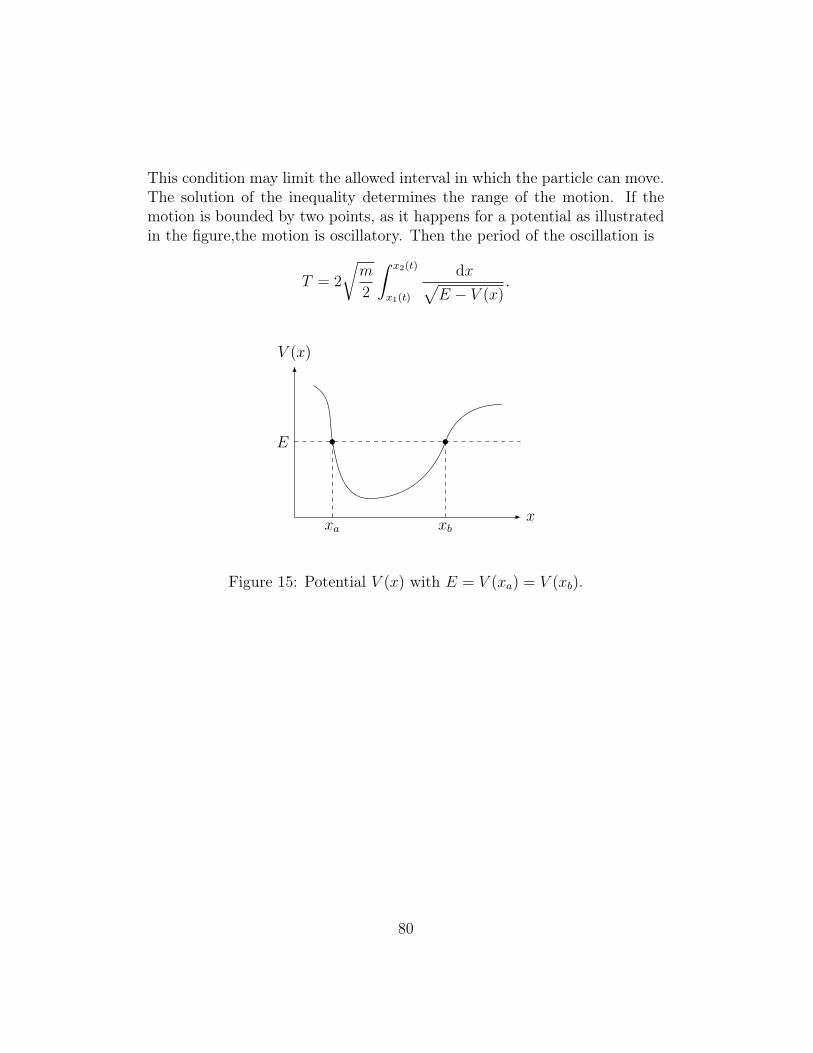
This condition may limit the allowed interval in which the particle can move.The solution of the inequality determines the range of the motion. If themotion is bounded by two points, as it happens for a potential as illustratedin the figure,the motion is oscillatory. Then the period of the oscillation is
T = 2
√m
2
∫ x2(t)
x1(t)
dx√E − V (x)
.
x
V (x)
E
xa xb
Figure 15: Potential V (x) with E = V (xa) = V (xb).
80

UNEDITED
81
9 Two-body problemIn this chapter we will discuss the interaction of two particles with massesm1 and m2, assuming that the force which exerts on each other depends onlyon their relative distance. The Lagrangian which describes such a system is
L =1
2m1r
21 +
1
2m2r
22 − V (|r1 − r2|).
We need to find the trajectories r1 = r1(t) and r2 = r2(t) of the two particles.We shall see that the symmetry of the problem simplifies this task.A first simplification we can make is to use a clever frame of reference. Thisis the, so called, center of mass frame in which the total momentum of allparticles in a system is zero. To determine this frame, we first find the averageposition of the masses:
R =
∑imiri∑imi
=m1r1 +m2r2
m1 +m2
. (9.1)
We also define the distance vector of the two particles. Assuming that m2 >m1, we define conventionally:
r = r1 − r2. (9.2)
We can express the position vectors of the two particles in terms of r and R.After a little algebra, we find:
r1 = R +m2
m1 +m2
r (9.3)
r2 = R− m1
m1 +m2
r. (9.4)
In terms of the (r, R) variables, the Lagrangian becomes:
L =1
2(m1 +m2)R2 +
1
2µr2 − V (r), (9.5)
where r ≡ |r| and µ is the reduced mass
µ =m1m2
m1 +m2
. (9.6)
82
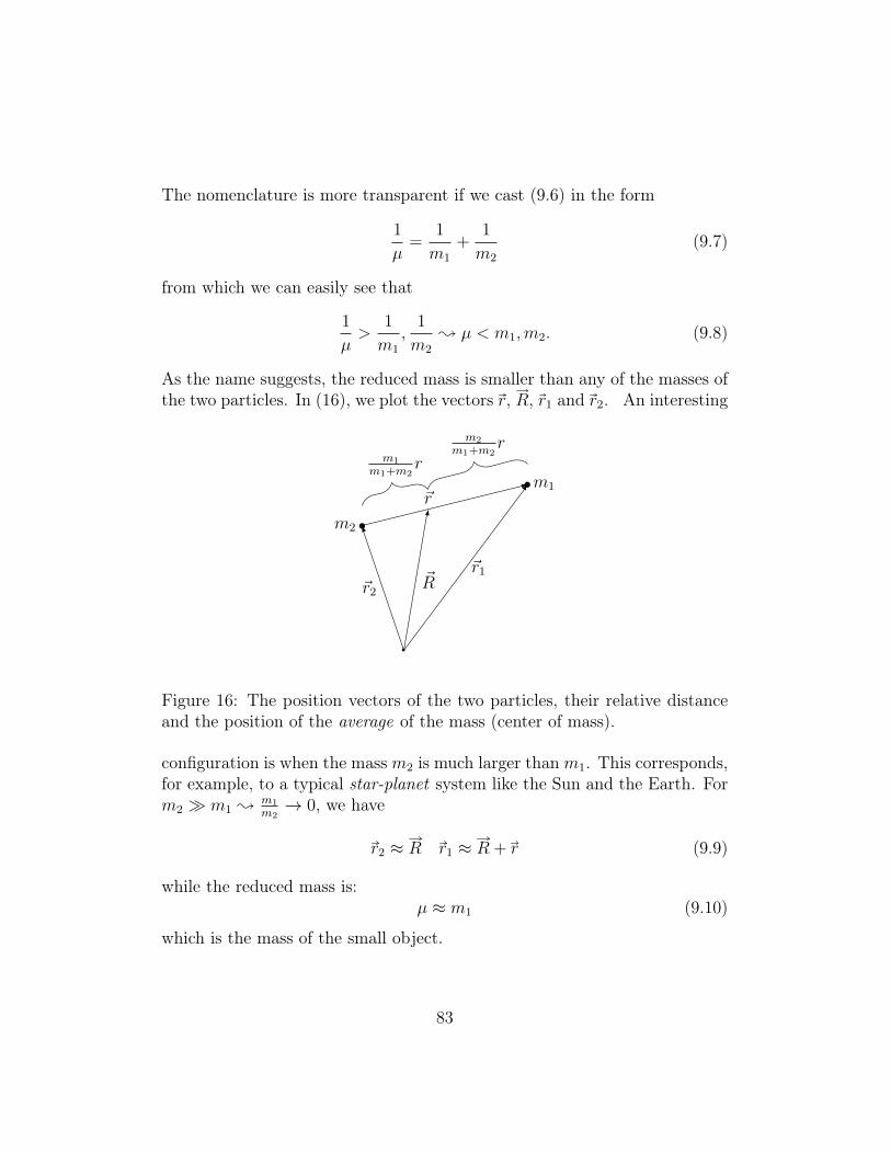
The nomenclature is more transparent if we cast (9.6) in the form
1
µ=
1
m1
+1
m2
(9.7)
from which we can easily see that
1
µ>
1
m1
,1
m2
; µ < m1,m2. (9.8)
As the name suggests, the reduced mass is smaller than any of the masses ofthe two particles. In (16), we plot the vectors r, R, r1 and r2. An interesting
~r2
m2
m1
~r1~R
~r
m1
m1+m2r
m2
m1+m2r
Figure 16: The position vectors of the two particles, their relative distanceand the position of the average of the mass (center of mass).
configuration is when the massm2 is much larger thanm1. This corresponds,for example, to a typical star-planet system like the Sun and the Earth. Form2 m1 ;
m1
m2→ 0, we have
r2 ≈ R r1 ≈ R + r (9.9)
while the reduced mass is:µ ≈ m1 (9.10)
which is the mass of the small object.
83

Let us now observe the structure of the Lagrangian of (9.8). We no-tice that the coordinates of the center of mass vector R ≡ (Rx, Ry, Rz) donot appear in the Lagrangian, but only the velocities R = (Rx, Ry, Rz) do.Therefore, the velocity of the center of mass must be constant:
R = const.. (9.11)
Indeed, we recall that
∂L
∂Rx
= 0 ;d
dt
∂L
∂Rx
= 0 ;d
dt[(m1+m2)Rx] = 0 ; Rx = const.. (similarly for Ry, Rz).
We can now exercise our freedom to choose our frame of reference such asthe center of mass is stationary:
R = 0. (9.12)
In this frame, the Lagrangian takes the form:
L =1
2µr2 − V (r). (9.13)
We have turned the two-body problem into a dual problem of a single particlewith “mass” equal to the reduced mass and a “position” the original distancevector of the two particles.The potential in (9.13) does not depend on the direction of r but only onits magnitude. Therefore, we expect the Lagrangian to be symmetric underrotations:
r → r′ = δφ× r. (9.14)
Then, the angular-momentum
M = r × P (9.15)
withP =
(∂L
∂x,∂L
∂y,∂L
∂z
)= µ(x, y, z) = µr (9.16)
is conserved:
d
dtM = 0 ; r × P = µ(r × r) = const.. (9.17)
84
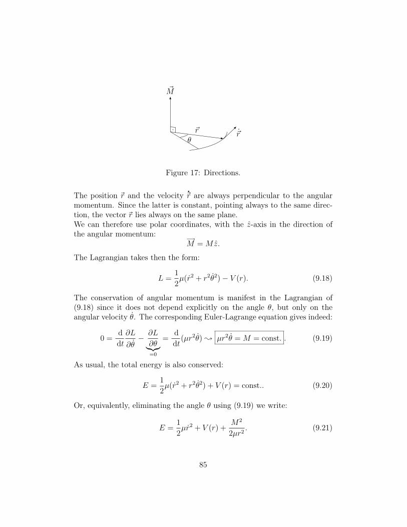
~M
~rθ
~r
Figure 17: Directions.
The position r and the velocity r are always perpendicular to the angularmomentum. Since the latter is constant, pointing always to the same direc-tion, the vector r lies always on the same plane.We can therefore use polar coordinates, with the z-axis in the direction ofthe angular momentum:
M = Mz.
The Lagrangian takes then the form:
L =1
2µ(r2 + r2θ2)− V (r). (9.18)
The conservation of angular momentum is manifest in the Lagrangian of(9.18) since it does not depend explicitly on the angle θ, but only on theangular velocity θ. The corresponding Euler-Lagrange equation gives indeed:
0 =d
dt
∂L
∂θ− ∂L
∂θ︸︷︷︸=0
=d
dt(µr2θ) ; µr2θ = M = const. . (9.19)
As usual, the total energy is also conserved:
E =1
2µ(r2 + r2θ2) + V (r) = const.. (9.20)
Or, equivalently, eliminating the angle θ using (9.19) we write:
E =1
2µr2 + V (r) +
M2
2µr2. (9.21)
85
Exercise 9.1. Verify that by taking the time derivative of (9.20) or (9.21)
dE
dt= 0
you can obtain the second equation of motion
d
dt
∂L
∂r− ∂L
∂r= 0. (9.22)
We can interpret (9.21) as the energy of a particle with mass µ movingin one only dimension and a potential
Veff(r) = V (r) +M2
2µr2︸ ︷︷ ︸”centrifugalenergy”
. (9.23)
Let us rewrite (9.21) in the form:
1
2µr2 = E − Veff(r) = E − M2
2µr2− V (r). (9.24)
The kinetic energy on the l.h.s. must be positive:
1
2µr2 ≥ 0 ; E − Veff(r) ≥ 0. (9.25)
The motion is therefore restricted to distances for which the total energyexceeds the effective potential energy Veff . The extrema of the motion arethe solutions of the equation
E = Veff(r). (9.26)
This can yield different types of trajectories:
Example 9.1. In figure (18), the motion is restricted in a finite range ofdistances in between [rmin, rmax].
Example 9.2. In figure (19), the energy is larger than Veff(r) up to infinitedistances.
86
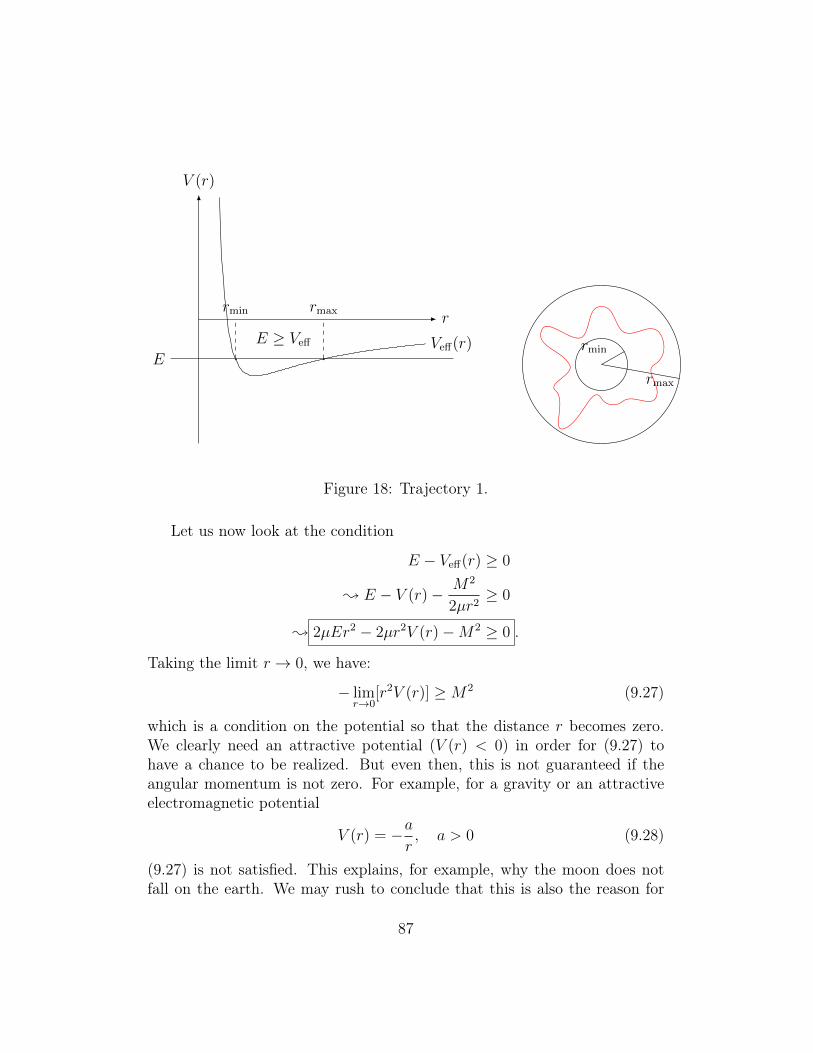
r
V (r)
Veff(r)
rmin rmax
E ≥ Veff
Ermin
rmax
Figure 18: Trajectory 1.
Let us now look at the condition
E − Veff(r) ≥ 0
; E − V (r)− M2
2µr2≥ 0
; 2µEr2 − 2µr2V (r)−M2 ≥ 0 .
Taking the limit r → 0, we have:
− limr→0
[r2V (r)] ≥M2 (9.27)
which is a condition on the potential so that the distance r becomes zero.We clearly need an attractive potential (V (r) < 0) in order for (9.27) tohave a chance to be realized. But even then, this is not guaranteed if theangular momentum is not zero. For example, for a gravity or an attractiveelectromagnetic potential
V (r) = −ar, a > 0 (9.28)
(9.27) is not satisfied. This explains, for example, why the moon does notfall on the earth. We may rush to conclude that this is also the reason for
87
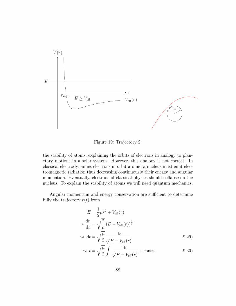
r
V (r)
Veff(r)rmin
E ≥ Veff
E
rmin
Figure 19: Trajectory 2.
the stability of atoms, explaining the orbits of electrons in analogy to plan-etary motions in a solar system. However, this analogy is not correct. Inclassical electrodynamics electrons in orbit around a nucleus must emit elec-tromagnetic radiation thus decreasing continuously their energy and angularmomentum. Eventually, electrons of classical physics should collapse on thenucleus. To explain the stability of atoms we will need quantum mechanics.
Angular momentum and energy conservation are sufficient to determinefully the trajectory r(t) from
E =1
2µr2 + Veff(r)
;dr
dt=
√2
µ(E − Veff(r))
12
; dt =
õ
2
dr√E − Veff(r)
(9.29)
; t =
õ
2
∫dr√
E − Veff(r)+ const.. (9.30)
88
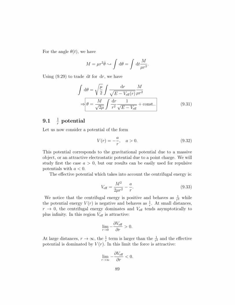
For the angle θ(t), we have
M = µr2θ ;
∫dθ =
∫dtM
µr2.
Using (9.29) to trade dt for dr, we have∫dθ =
õ
2
∫dr√
E − Veff(r)
M
µr2
⇒ θ =M√2µ
∫dr
r2
1√E − Veff
+ const.. (9.31)
9.1 1r potential
Let us now consider a potential of the form
V (r) = −ar, a > 0. (9.32)
This potential corresponds to the gravitational potential due to a massiveobject, or an attractive electrostatic potential due to a point charge. We willstudy first the case a > 0, but our results can be easily used for repulsivepotentials with a < 0.
The effective potential which takes into account the centrifugal energy is:
Veff =M2
2µr2− a
r. (9.33)
We notice that the centrifugal energy is positive and behaves as 1r2
whilethe potential energy V (r) is negative and behaves as 1
r. At small distances,
r → 0, the centrifugal energy dominates and Veff tends asymptotically toplus infinity. In this region Veff is attractive:
limr→0−∂Veff
∂r> 0.
At large distances, r →∞, the 1rterm is larger than the 1
r2and the effective
potential is dominated by V (r). In this limit the force is attractive:
limr→∞−∂Veff
∂r< 0.
89
r
V (r)
M2
2µr2
−ar
Veff(r)
r0
Figure 20: Effective potential.
In the intermediate region the potential develops a minimum:
∂Veff
∂r
∣∣∣∣r=r0
; r0 =M2
µa. (9.34)
The shape of the potential is shown in Figure (20). To calculate the tra-jectory, we need to calculate the integral of (9.31) for Veff given by (9.33):
θ(r) =1√2µ
∫dr
r2
1√E − M2
2µr2+ a
r
+ const.. (9.35)
We can cast the above formula as
θ(r) =
∫dr
r2
1√−(
1r− 1
p
)2
+ ε2
p2
+ const. (9.36)
90
wherep ≡ M2
µa(9.37)
and
ε ≡
√1 +
2EM2
µa2. (9.38)
With the change of variables,
1
r=
1
p+e
pcosω (9.39)
the integral of (9.36) becomes
θ =
∫dω + const.
which leads toθ = ω + θ0. (9.40)
Thus, from (9.39) we find the trajectory
1
r=
1
p+e
pcos(θ − θ0)
or, equivalently:p
r= 1 + e cos(θ − θ0) . (9.41)
(9.41) describes the trajectory r = r(θ) for the distance of the two particles.As we can see, the trajectory depends on the value of the two parameters(e, p) which in term depend on the energy E and angular momentumM . Wewill find three types of trajectories, according to the following table. For the
e > 1 E > 0 hyperbola
e = 1 E = 0 parabola
e < 1 E < 0 ellipsis
91
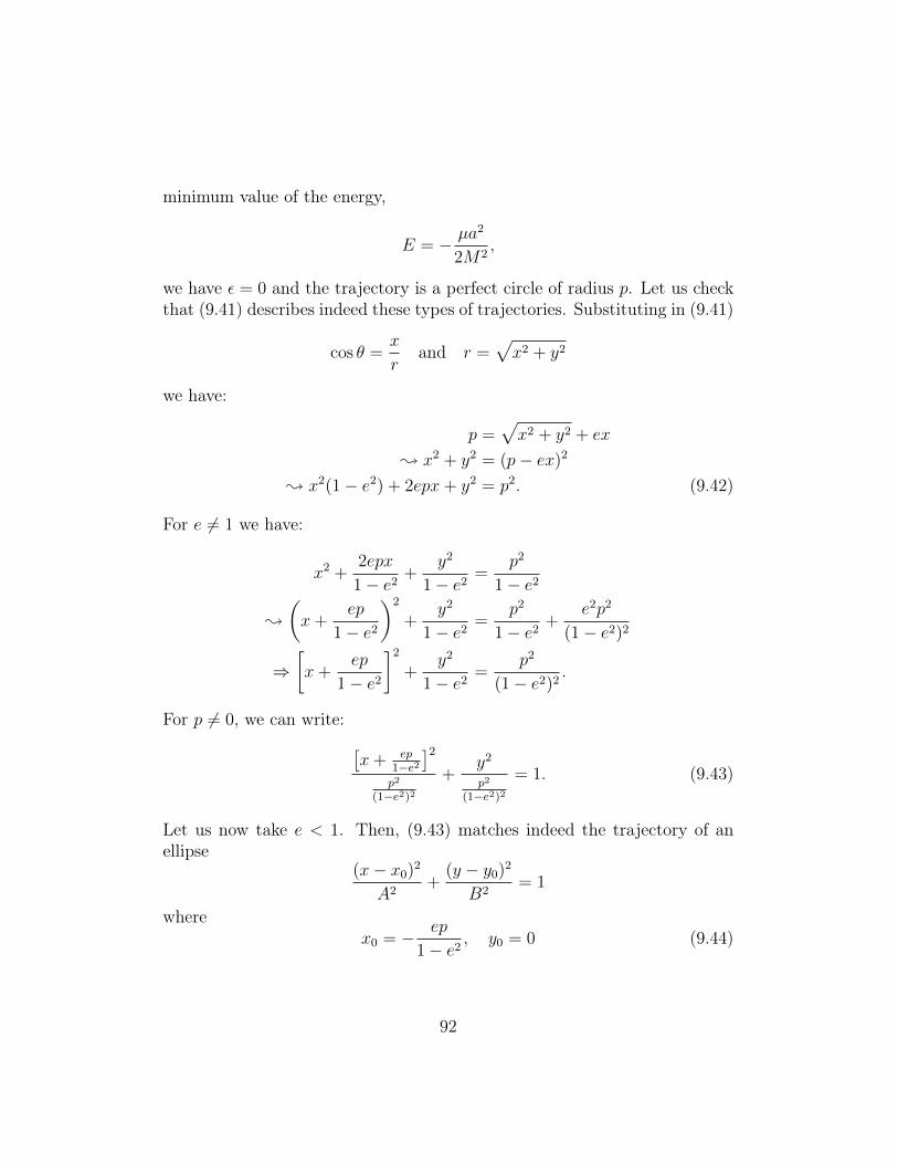
minimum value of the energy,
E = − µa2
2M2,
we have ε = 0 and the trajectory is a perfect circle of radius p. Let us checkthat (9.41) describes indeed these types of trajectories. Substituting in (9.41)
cos θ =x
rand r =
√x2 + y2
we have:
p =√x2 + y2 + ex
; x2 + y2 = (p− ex)2
; x2(1− e2) + 2epx+ y2 = p2. (9.42)
For e 6= 1 we have:
x2 +2epx
1− e2+
y2
1− e2=
p2
1− e2
;
(x+
ep
1− e2
)2
+y2
1− e2=
p2
1− e2+
e2p2
(1− e2)2
⇒[x+
ep
1− e2
]2
+y2
1− e2=
p2
(1− e2)2.
For p 6= 0, we can write: [x+ ep
1−e2]2
p2
(1−e2)2
+y2
p2
(1−e2)2
= 1. (9.43)
Let us now take e < 1. Then, (9.43) matches indeed the trajectory of anellipse
(x− x0)2
A2+
(y − y0)2
B2= 1
wherex0 = − ep
1− e2, y0 = 0 (9.44)
92
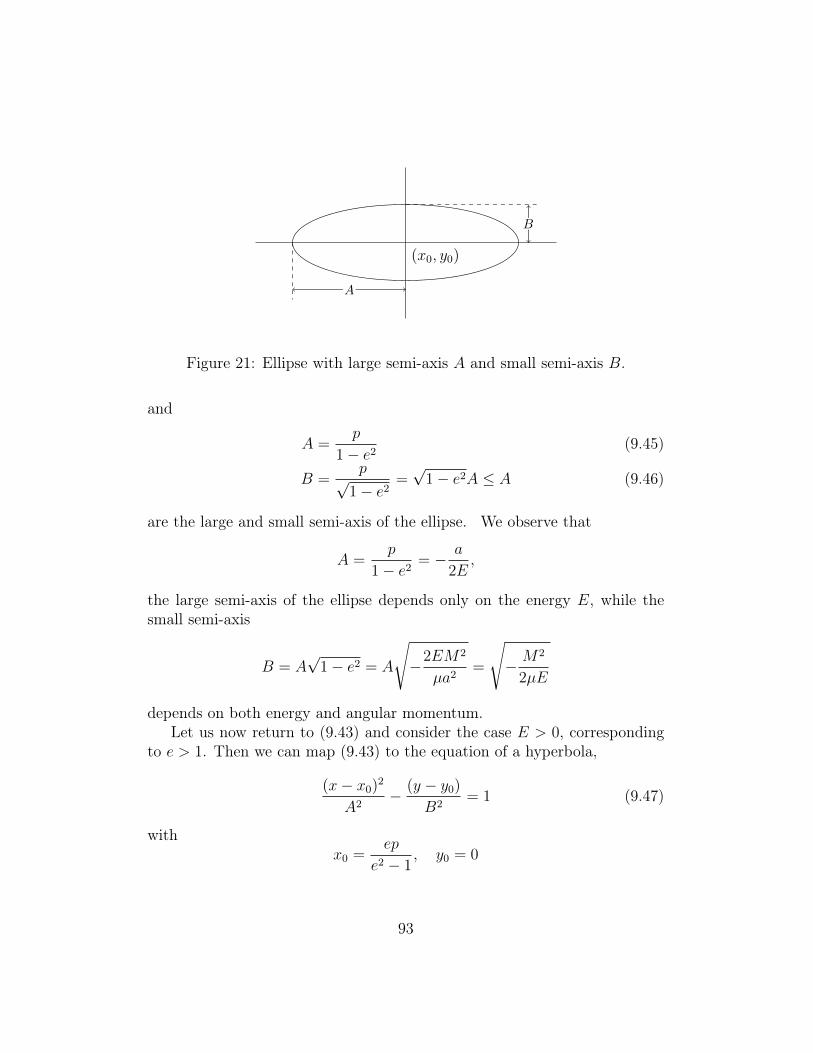
(x0, y0)
B
A
Figure 21: Ellipse with large semi-axis A and small semi-axis B.
and
A =p
1− e2(9.45)
B =p√
1− e2=√
1− e2A ≤ A (9.46)
are the large and small semi-axis of the ellipse. We observe that
A =p
1− e2= − a
2E,
the large semi-axis of the ellipse depends only on the energy E, while thesmall semi-axis
B = A√
1− e2 = A
√−2EM2
µa2=
√− M2
2µE
depends on both energy and angular momentum.Let us now return to (9.43) and consider the case E > 0, corresponding
to e > 1. Then we can map (9.43) to the equation of a hyperbola,
(x− x0)2
A2− (y − y0)
B2= 1 (9.47)
withx0 =
ep
e2 − 1, y0 = 0
93
and
A =p
e2 − 1(9.48)
B =p√e2 − 1
=√e2 − 1A (9.49)
We let the reader as an exercise to investigate the special cases of ε = 1 and
C =√B2 + A2
2A
2C
Figure 22: Hyperbola.
E = 0.
9.2 Laplace-Runge-Lenz vector
Consider the Lagrangian of a particle in a central arpotential:
L =1
2mr2 +
a
r. (9.50)
94
The Euler-Lagrange equations yield Newton’s law:
mr = −a rr3. (9.51)
Now let’s consider the cross product of the momentum and the angular mo-mentum
P ×M.
Differentiating with time, we have:
d
dt(P ×M) =
dP
dt×M
= − a
r3(r ×M)
= − a
r3
[r × (r × P )
]= −ma
r3
[r × (r × r)
]. (9.52)
Exercise 9.2. Prove the identity:
r × (r × r) = r(r · r)− r2r,
where2rr =
dr2
dt=
d
dt(r · r) = 2rr ; rr = rr.
Thus,
r × (r × r) = r3
(rr
r2− r r
r3
)= −r3 d
dt
(r
r
).
Returning to (9.52), we find:
d
dtP ×M = ma
d
dt
(r
r
);
d
dt
[P ×M − amr
r
]= 0.
Thus, the vector
A ≡ P ×M − r
rma = const. (9.53)
is conserved. The vector is known as the Laplace-Runge-Lenz vector.
95
It is easy to verify that the LRL vector is vertical to the angular momen-tum
A ·M = 0 (9.54)
and, thus, it must lay on the plane of the motion. We will see in late lecturesthat the LRL vector is conserved due to a special symmetry, owed to thespecial form (1
r) of the potential.
Exercise 9.3. Find the size and the orientation of the LRL vector for
(i) an elliptical orbit
(ii) a hyperbolic orbit.
It is important to note that any variations of the LRL vector indicatepossible deviations from Newton’s law of gravity. Thus, measurements ofA(t) as a function of time are stringent tests of Newton’s law. Such deviationsare expected, for example, in Einstein’s theory of General Relativity.
What is the symmetry giving use to the conservation law of LRL?
ri → ri + δkri
withδkri = εµ
(rirk −
1
2rirk − δik
(1
2r · r
))(9.55)
where we change all three ri’s simultaneously. From (9.55), we obtain:
δkri =εµ
2
[rirk − δikr2 − a
µ
rirkr3
+ δika
µ
1
r
]. (9.56)
The Lagrangian changes by:
δL = µr · δr − ar · δrr3
(9.55),(9.56)⇒ δkL = εd
dt
(µarkr
).
Then, we can use Noether’s theorem:
∂L
∂kriδkri − F = const.
⇒ A = P ×M − µarr
= const..
Exercise 9.4. Fill the gaps.
96
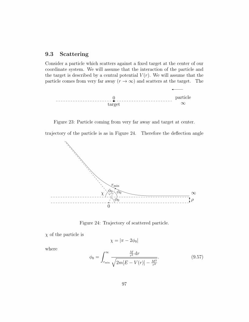
9.3 Scattering
Consider a particle which scatters against a fixed target at the center of ourcoordinate system. We will assume that the interaction of the particle andthe target is described by a central potential V (r). We will assume that theparticle comes from very far away (r →∞) and scatters at the target. The
0
target ∞particle
Figure 23: Particle coming from very far away and target at center.
trajectory of the particle is as in Figure 24. Therefore the deflection angle
ρ
0
φ0
φ0φ0χ
rmin
∞
Figure 24: Trajectory of scattered particle.
χ of the particle isχ = |π − 2φ0|
where
φ0 =
∫ ∞rmin
Mr2
dr√2m[E − V (r)]− M2
r2
. (9.57)
97
To compute rmin, we note that
1
2mr2 = E − V (r)− M2
2mr2(9.58)
and r = 0 for r = rmin leads to
E − V (rmin) +M2
2mr2min
= 0. (9.59)
Let us now express the energy and the angular momentum in terms of thevelocity of the particle at infinity, v∞, and the impact parameter ρ. We have:
E =1
2mv2∞ (9.60)
M = mρv∞. (9.61)
Thus:φ0 =
∫ ∞rmin
ρr2
dr√1− ρ2
r2− 2V
mv2∞
. (9.62)
Let us now consider a beam of particles with the same velocity at infin-ity which scatter on the target. The beam particles have different impactparameters. Thus they scatter at different angles. We denote with
dN ≡ # of scattered particles in between χ and χ+ dχ
unit time. (9.63)
This rate depends on the flux of particles in the incoming beam. We definethe flux as
n ≡ # of incoming particlestime · area
.
We can measure experimentally the ratio
dσ =dN
n. (9.64)
This ratio is called the effective scattering cross-section. It has units of areand it characterizes the physical properties of the scattering process and thepotential. Let’s assume that particles with impact factor ρ(χ) to ρ(χ) + dρscatter in between χ and dχ. Then
98
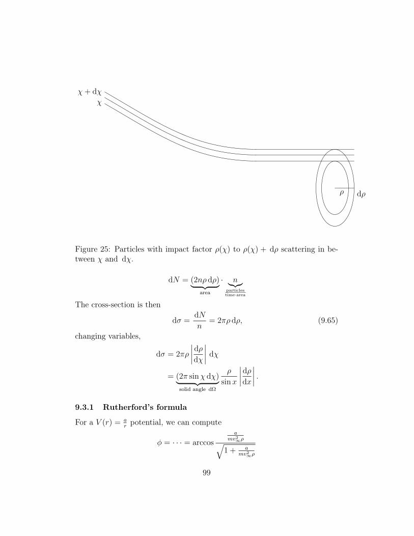
ρ dρ
χ+ dχ
χ
Figure 25: Particles with impact factor ρ(χ) to ρ(χ) + dρ scattering in be-tween χ and dχ.
dN = (2nρ dρ)︸ ︷︷ ︸area
· n︸︷︷︸particlestime·area
The cross-section is then
dσ =dN
n= 2πρ dρ, (9.65)
changing variables,
dσ = 2πρ
∣∣∣∣dρdχ
∣∣∣∣ dχ
= (2π sinχ dχ)︸ ︷︷ ︸solid angle dΩ
ρ
sinx
∣∣∣∣dρdx
∣∣∣∣ .9.3.1 Rutherford’s formula
For a V (r) = arpotential, we can compute
φ = · · · = arccos
amv2∞ρ√
1 + amv2∞ρ
99
Exercise 9.5. Verify this result.
; ρ2 =a2
m2v4∞
cot2 χ
2
(φ0 =
π − χ2
).
Then dρ2 = 2ρ dρ is easy to compute. We then obtain
dσ = πa
(2mv2∞)2
dΩ
sin4 χ2
.
100
10 Virial TheoremConsider N particles interacting via Newton’s law. If positions are bounded,
〈T 〉 = −〈V 〉2.
Consider
G =∑i
Pi · ri
;dG
dt=∑i
dPidt· ri +
∑i
Pi ·dridt
=∑i
Fi · ri + 2T
;d
dt
∑i
Pi · ri = 2T +∑i
Fi · ri.
The time average is
〈F 〉 =1
τ
∫ τ
0
F (t) dt.
Thus
1
τ
∫ τ
0
dtd
dt
∑i
Pi · ri = 2 〈T 〉+
⟨∑i
Fi · ri
⟩
⇒ 2 〈T 〉+
⟨∑i
Fi · ri
⟩= G(τ)−G(0).
Assume that the motions are bounded. Then G(τ) is bounded as well. If wethen take τ →∞, we have
G(τ)−G(0)
τ
τ→∞−→ 0.
Then
〈T 〉 = −1
2
⟨∑i
Fi · ri
⟩.
101
This is known as the virial theorem.
For a single particle,
〈T 〉 = −1
2
⟨1∑i=1
Fi · ri
⟩= −1
2
⟨(−∇V ) · r
⟩.
For a central potential, we get
〈T 〉 =1
2
⟨∂V
∂rr
⟩.
If V = arn, we have∂V
∂r= narn = nV , thus:
〈T 〉 =n
2〈V 〉 .
For a gravity or electrostatic potential, we have:
n = −1 ; 〈T 〉 = −〈V 〉2
.
102
For many particles and a 1rpotential:
−∑i
(∇iV ) · ri = −∑i
ri∇1
2
∑k 6=l
a
|rk − rl|
= +21
2
∑i
ri∇∑l 6=i
a(ri − rl)|ri − rl|3
= +∑l<i
a(ri − rl) · ri|ri − rl|3
+∑i<l
a(ri − rl) · ri|ri − rl|3
= +∑l<i
a(ri − rl) · ri|ri − rl|3
+∑l<i
a(rl − ri) · rl|ri − rl|3
= +∑l<i
a [(ri − rl) · ri − (ri − rl) · rl]|ri − rl|3
= +∑l<i
a(ri − rl)2
|ri − rl|3
= +∑l<i
a
|ri − rl|= V
Thus we have proven that
〈T 〉 = −1
2〈V 〉 .
Application in astrophysics
Velocities
measured 〈T 〉 = 12〈V 〉
Distances
“measured”+
geometricalsymmetries
Estimate ofmass. Dark matter!
103
11 Oscillations
11.1 Small Oscillations
ROUGH DRAFT
Oscillations can occur in potentials with stable points of equilibrium. Forsystems with one degree of freedom, this means that for a potential V (q) itexists a q0 with
∂V
∂q0
> 0 and − ∂V
∂q0
< 0.
This returns the particle to q0. The Taylor expansion for this potential is
V (q) = V (q0) +:0
V ′(q0) (q − q0) +1
2V ′′(q0)(q − q0)2 +O
[(q − q0)3
].
If we set V (q0) = 0, which is the shifting value of the potential by a constant,we need to find
V (k) ≈ 1
2k(q − q0)2 with k > 0.
For a simple particle, we have
L ≈ 1
2mx2 − 1
2kx2
which gives us the following Euler-Lagrange equations:
d
dt
∂L
∂x− ∂L
∂x= 0
; mx+ kx = 0
; x+k
mx = 0
x+ ω2x = 0 with ω =
√k
m.
Then the solution isx = c1 cosωt+ c2 sinωt.
Indeed,
x = ω [−c1 sinωt+ c2 cosωt]
x = ω2 [−c1 cosωt− c2 sinωt] = −ω2x .
104
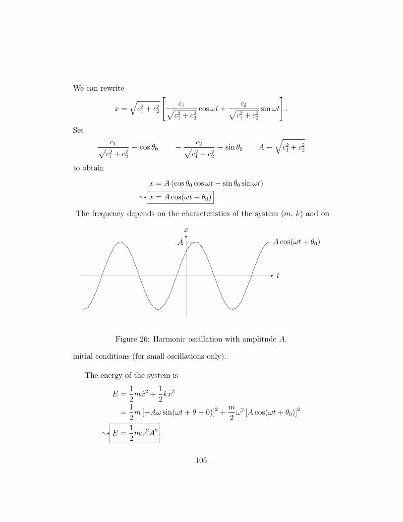
We can rewrite
x =√c2
1 + c22
[c1√c2
1 + c22
cosωt+c2√c2
1 + c22
sinωt
].
Setc1√c2
1 + c22
≡ cos θ0 − c2√c2
1 + c22
≡ sin θ0 A ≡√c2
1 + c22
to obtain
x = A (cos θ0 cosωt− sin θ0 sinωt)
; x = A cos(ωt+ θ0) .
The frequency depends on the characteristics of the system (m, k) and on
t
x
A cos(ωt+ θ0)A
Figure 26: Harmonic oscillation with amplitude A.
initial conditions (for small oscillations only).
The energy of the system is
E =1
2mx2 +
1
2kx2
=1
2m [−Aω sin(ωt+ θ − 0)]2 +
m
2ω2 [A cos(ωt+ θ0)]2
; E =1
2mω2A2 .
105
Thus,
x =
√2E
mωcos(ωt+ θ0).
The amplitude A of the oscillation depends on the energy, as expected.
It is often convenient to “complexify” the amplitude:
A = |A|eiθ0 .
Then,x = Re
(Aeiωt
).
Indeed,
x = Re(|A|ei(ωt+θ0)
)= |A| cos(ωt+ θ0).
11.2 Forced Oscillations
Exert an external time-dependent force on an oscillatory system, then
V ≈ 1
2kx2 + Vex(x, t)
≈ 1
2kx2 +
[∂Vex
∂x
]x=0
+ Vex(0, t)︸ ︷︷ ︸can be written
as a time derivative
.
Thus,
V (x, t) ≈ 1
2kx2 − xF (t)
L =1
2mx2 − 1
2kx2 + xF (t) (11.1)
which yields the following equation of motion:
d
dt
∂L
∂x− ∂L
∂x= 0
; mx = −kx+ F (t)
; x+ ω2x =F (t)
m. (11.2)
106
For the general solution, we set
ζ = x+ iωx (11.3)
ζ = x+ iωx
−iωζ = −iωx+ ω2x
which gives usd
dtζ − iωζ =
F (t)
m. (11.4)
Set now ζ = eiωty, then
eiωty + iωζ − iωζ =F (t)
m
⇒ y =e−iωtF (t)
m
⇒ y =
∫dte−iωtF (t)
m+ y0
⇒ ζ = eiωt
[y0 +
∫dte−iωtF (t)
m
]. (11.5)
The energy of the system is
E =1
2mx2 +
1
2kx2
=1
2m(x2 + ω2x2) =
1
2mζ2
=1
2m(x− iωx)(x+ iωx)
⇒ E =1
2m |ζ(t)|2 (11.6)
The energy is not conserved. Assuming that we “pump” all energy in viaF (t), we have for the energy of the system after infinite time,
E =1
2m |ζ(+∞)|2
=1
2m
∣∣∣∣∫ ∞−∞
dtF (t)
me−iωt + y0
∣∣∣∣2 . (11.7)
107
where the last integral can be recognized as the Fourier transform of the force.
Let us now work out explicitly the trajectory for
F (t) = f cos(γt+ β). (11.8)
Then
ζ(t) = e+iωt
[∫dt e−iωt cos(γt+ β)
f
m+ y0
]⇒ ζ(t) = eiωty0 +
fγ
m(γ2 − ω2)sin(γt+ β)− i
fω
m(γ2 − ω2)cos(γt+ β)
(11.9)
But
ζ(t) = x+ iωx
⇒ e+iωtζ(t) =d
dt(eiωtx)
⇒ x = e−iωt
(c+
∫dt e+iωtζ(t)
). (11.10)
Performing the integrations, we have
x(t) = − f/m
γ2 − ω2cos(γt+ β) + Ae−iωt.
The real part of the solution is
x(t) = |A| cos(ωt+ θ0) +f/m
ω2 − γ2cos(γt+ β) . (11.11)
The first term is the solution of the homogeneous equation and it is the sameas when the external force is absent. The second term is new. It is also anoscillatory function of time, but with the frequency of the external force.
The amplitude of the oscillation increases as the frequency of the externalforce γ approaches the value of the characteristic frequency of the system ω.This phenomenon is called resonance. To calculate the motion at exactlyω = γ, we write:
x(t) = |B| cos(ωt+ θ0) +f
m(ω2 − γ2)[cos(γt+ β)− cos(ωt+ beta)] (11.12)
108
At γ → ω, we have
x(t) = |B| cos(ωt+ θ0) +f
2mωt sin(ωt+ β) (11.13)
Notice that the amplitude increases with time. The above formula is notvalid if our Lagrangian of (11.1) is only valid for small x, since after sometime the amplitude of the oscillation becomes large.
Let us now complexify (11.11):
x = A1eiωt + A2eiγt
=[A1 + A2ei(γ−ω)t
]eiωt. (11.14)
For γ = ω + ε, close the resonance with ε being small, we can write
x(t) =[A1 + A2eiεt
]eiωt
= C(t)eiωt (11.15)
where the “amplitude” C(t) varies very slowly in time. Setting
A1 = |A1|eiθ1 and A2 = |A2|eiθ2 ,
we obtain:
|C(t)|2 = |A1|2 + |A2|2 + 2|A1||A2| cos(θ2 − θ1 + εt)
⇒ (|A1||A2|)2 ≤ |C(t)|2 ≤ (|A1||A2|)2
⇒ ||A1| − |A2|| ≤ C(t) ≤ |A1|+ |A2|. (11.16)
The amplitude varies periodically in between two values. This phenomenonis known as beats.
11.3 Oscillations of systems with many degrees of free-dom
We will now study oscillatory behaviour in systems with many degrees offreedom. A Lagrangian describing such a system is of the form
L =1
2
∑i,j
(mijxixj − kijxixj) (11.17)
109

where
mij = mji (11.18)kij = kji. (11.19)
To compute the equations of motion, we need first
∂L
∂xi=∑j
mijxj (11.20)
∂L
∂xi=∑j
kijxj. (11.21)
The Euler-Lagrange equations give then:∑j
(mijxj + kijxj) = 0, i = 1, . . . , N. (11.22)
This is a system of N differential equations with N unknowns. We can set
xj = Ajeiωt (11.23)
(and only need to remember to keep the real part of this expression at theend of the calculation).Substituting into (11.22), we obtain:∑
j
(kij − ω2mij)Aj = 0 (11.24)
or, in a matrix formk11 − ω2m11 k12 − ω2m12 . . .k21 − ω2m21 k22 − ω2m22 . . .
...... . . .
A1
A2...
=
0...0
. (11.25)
The condition for the system to have oscillatory solutions of the form of(11.23) is then
det(kij − ω2mij) = 0 (11.26)
110
The solutions of (11.26), if they exist, are real and positive. Indeed:∑j
(kij −mijω2)Aj = 0
;∑i,j
(kij −mijω2)A?iAj = 0
⇒ ω2 =
∑i,j kijA
?iAj∑
i,jmijA?iAj
=
∑i,j kjiA
?iAj∑
i,jmjiA?iAj
=
∑i,j kijAiA
?j∑
i,jmijAiA?j=(ω2)?
; ω2 is real.
Notice also that∑i,j
AiA?j =
∑i,j
kij(ai + ibi)(aj − ibj)
=∑i,j
kij(aiaj + bibj) + i
:0∑i,j
kij︸︷︷︸symmetric
(biaj − aibj)
=∑i,j
kij(aiaj + bibj) ≥ 0.
The roots of ω2a of (11.26) give the characteristic frequencies (eigenfrequen-
cies) of the system. To construct solutions xj(t) after this step becomes asimple exercise in Linear Algebra to find the eigenvectors corresponding toeach ωa. Let us assume, for simplicity, that there is no degeneracy. Then thesolutions are
xj(t) =∑a
∆jaθa(t) (11.27)
with ∆ja the minors of the determinant and
θa(t) = Re [Caexp(iωat)] . (11.28)
We can regard the equation
xj =∑a
∆jaθa
111
as a change from one set of generalized coordinates to another. The θacoordinates satisfy the differential equations
θa + ω2aθa = 0 (11.29)
and are called normal coordinates. They describe independent oscillators. Innormal coordinates, the Lagrangian takes the form
L =∑a
1
2ma(θ
2a − ω2
aω2a).
Exercise 11.1. Consider the Lagrangian
L =1
2
[x2
1 + 2x1x2 + x22 − 3x2
1 − 4x22 + 2x1x2
].
Find the eigenfrequencies and normal coordinates.
11.4 Damped Oscillations
We now consider oscillatory systems with some friction losses. The equationfo motion for the simplest one-dimensional oscillator is
mx+ kx+ αx = 0
or, equivalently,x+ ω2
0x+ 2λx = 0
withω2
0 =k
mand 2λ =
a
m.
The solution is of the formx(t) = ekt,
then
k2 + ω20 + 2λk = 0
; (k + λ)2 = λ2 − ω20
⇒ k = −λ±√λ2 − ω2
0
112
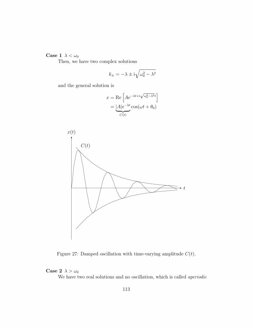
Case 1 λ < ω0
Then, we have two complex solutions
k± = −λ± i√ω2
0 − λ2
and the general solution is
x = Re[Ae−λt+i
√ω20−λ2t
]= |A|e−λt︸ ︷︷ ︸
C(t)
cos(ωt+ θ0)
t
x(t)
C(t)
Figure 27: Damped oscillation with time-varying amplitude C(t).
Case 2 λ > ω0
We have two real solutions and no oscillation, which is called aperiodic
113
damping :x = e−λt
[c1e−√λ2−ω2
0t + c2e+√λ2−ω2
0t].
For many degrees of freedom, the frictional forces take the form:
fi = −∑j
αijxj.
Then, we can write
fi = −∂F∂xi
with F =1
2
∑i,j
αijxixj.
Then, the equations of motion can originate from
d
dt
∂L
∂xi− ∂L
∂xi= −∂F
∂xi.
The function F is known as the dissipative function.Let us now compute the energy change vote:
dE
dt=
d
dt
(∑i
xi∂L
∂xi− L
)
= x∂L
∂xi− dL
dt+ xi
d
dt
∂L
∂xi
= x∂L
∂xi− ∂L
∂xixi −
∂L
∂xixi + xi
d
dt
∂L
∂xi
= xi
[d
dt
∂L
∂xi− ∂L
∂xi
]= −xi
∂F
∂xi= −2F.
For the system to lose energy, we require that
F > 0.
114
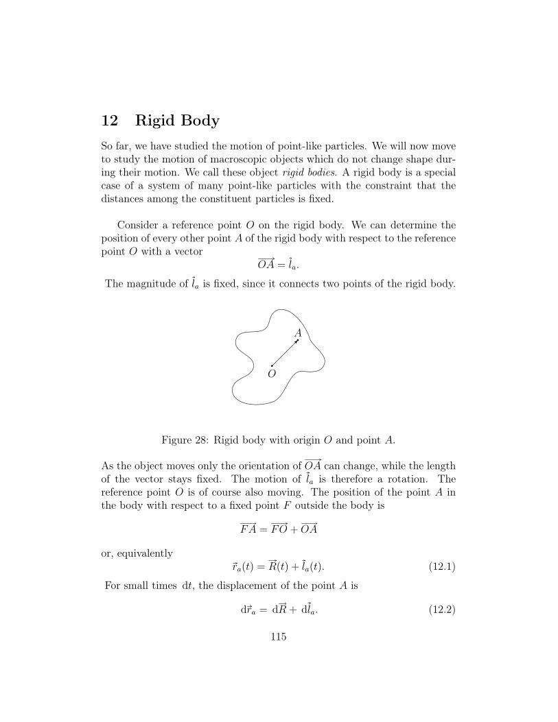
12 Rigid BodySo far, we have studied the motion of point-like particles. We will now moveto study the motion of macroscopic objects which do not change shape dur-ing their motion. We call these object rigid bodies. A rigid body is a specialcase of a system of many point-like particles with the constraint that thedistances among the constituent particles is fixed.
Consider a reference point O on the rigid body. We can determine theposition of every other point A of the rigid body with respect to the referencepoint O with a vector
OA = la.
The magnitude of la is fixed, since it connects two points of the rigid body.
O
A
Figure 28: Rigid body with origin O and point A.
As the object moves only the orientation of OA can change, while the lengthof the vector stays fixed. The motion of la is therefore a rotation. Thereference point O is of course also moving. The position of the point A inthe body with respect to a fixed point F outside the body is
FA = FO +OA
or, equivalentlyra(t) = R(t) + la(t). (12.1)
For small times dt, the displacement of the point A is
dra = dR + dla. (12.2)
115

O
A~la(t1)
O
A~la(t2)
F
~R(t1)
~r(t1) ~R(t2)
~r(t2)
Figure 29: Same body with different orientation.
We can write the change dla as an infinitesimal rotation
dla = dφ× la. (12.3)
Thus, we have thatdradt
=dR
dt+
dφ
dt× la . (12.4)
This is an equation which relates the velocity of a particle A in the rigidbody to the velocity of a reference point O and the angular velocity
ω =dφ
dt(12.5)
of a point A with respect to the fixed point O. All points in a rigid body ro-tate simultaneously, as they are required to have fixed distances. Therefore,the angular velocity ω is common to all particles.
Let us call
V ≡ dR
dt(12.6)
the velocity of the reference point O.We will assume that a body is composed of a = 1, . . . , N particles with
116
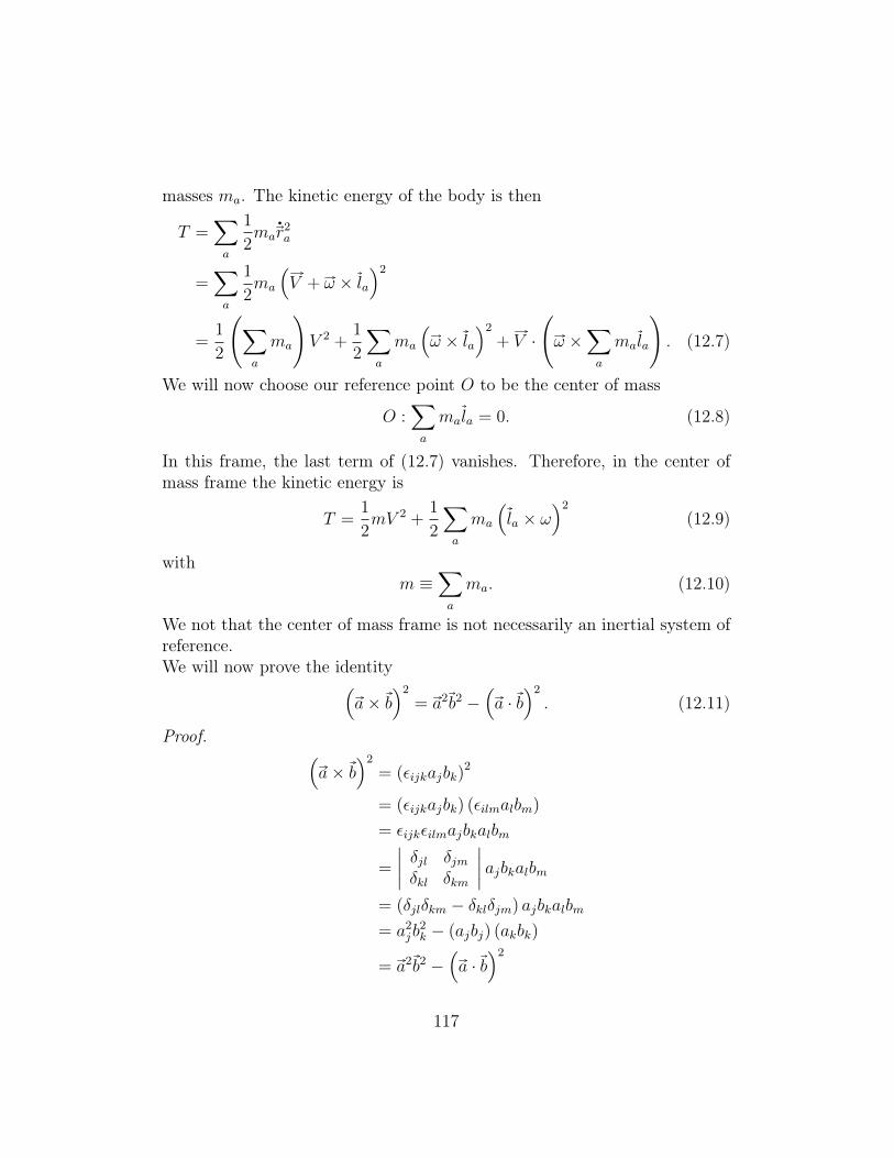
masses ma. The kinetic energy of the body is then
T =∑a
1
2mar
2a
=∑a
1
2ma
(V + ω × la
)2
=1
2
(∑a
ma
)V 2 +
1
2
∑a
ma
(ω × la
)2
+ V ·
(ω ×
∑a
mala
). (12.7)
We will now choose our reference point O to be the center of mass
O :∑a
mala = 0. (12.8)
In this frame, the last term of (12.7) vanishes. Therefore, in the center ofmass frame the kinetic energy is
T =1
2mV 2 +
1
2
∑a
ma
(la × ω
)2
(12.9)
withm ≡
∑a
ma. (12.10)
We not that the center of mass frame is not necessarily an inertial system ofreference.We will now prove the identity(
a× b)2
= a2b2 −(a · b
)2
. (12.11)
Proof. (a× b
)2
= (εijkajbk)2
= (εijkajbk) (εilmalbm)
= εijkεilmajbkalbm
=
∣∣∣∣ δjl δjmδkl δkm
∣∣∣∣ ajbkalbm= (δjlδkm − δklδjm) ajbkalbm
= a2jb
2k − (ajbj) (akbk)
= a2b2 −(a · b
)2
117
Therefore, the “rotational” term of the kinetic energy in (12.9) becomes
1
2
∑a
ma
(ω × la
)2
=1
2
∑a
ma
(ω2l2a −
(ω · la
)2). (12.12)
Let us now write the above in terms of the Cartesian components of theposition vectors
la ≡ (la1, la2, la3) ≡ (lai) .
We have
ω2l2a −(ω · la
)2
= (ωiωi) l2a − (ωilai)
2
= ωiωjδijl2a − ωiωjlailaj
=(δijl
2a − lailaj
)ωiωj (12.13)
Therefore, the kinetic energy takes the form
T =1
2mV 2 +
1
2Iijωiωj (12.14)
where m ≡∑
ama is the total mass of the rigid body and Iij is the so calledtensor of inertia.
12.1 Tensor of inertia
The tensor of inertia is characteristic of the geometry and mass distributionof the rigid body. From its definition,
Iij ≡∑a
ma
(l2i δij − lailaj
)(12.15)
we see that it is a symmetric tensor:
Ijk = Ikj.
It therefore consists of six components. In a matrix notation, the tensor ofinertia is
Ijk =∑a
l2a2 + l2a3 −la1la2 −la1la3
−la1la2 l2a1 + l2a3 −la2la3
−la1la3 −la2la3 l2a1 + l2a2
ma. (12.16)
118
Using standard linear algebra methods, we can diagonalize this matrix. Thediagonalization corresponds to a change of axes for the vectors la. The axesfor which the tensor of inertia is diagonal are called principal axes.I11 I12 I13
I21 I22 I23
I31 I32 I33
Rotation−→of axes
I1 0 00 I2 00 0 I3
. (12.17)
The eigenvalues I1, I2, I3 are called the principal moments of inertia.
Exercise 12.1. Demonstrate that principal axes always exist.
We can prove the following inequalities:
I1 + I2 ≥ I3
I2 + I3 ≥ I1
I3 + I1 ≥ I2. (12.18)
Indeed,
I1 + I2 =∑a
(l2a2 + l2a3 + l2a1 + l2a3
)≥∑a
ma
(l2a1 + l2a2
)= I3.
In the definition of the tensor of inertia of (12.16), the position vectors of therigid body points la are measured with respect to the center of mass. Let usnow consider an analogous expression
I ′ij ≡∑a
ma
(r2aδij − rairaj
)(12.19)
where the vectors ra ≡ la + c are measured with respect to a different point.Then,
I ′ij =∑a
ma
((la + c
)2
δij − (lai + ci) (laj + cj)
)
=∑a
ma
(l2aδij − lailaj
)+
(∑a
ma
)(c2δij − cicj
)+ 2
(∑a
mala
)· cδij
(∑a
malai
)cj −
(∑a
malaj
)ci.
119

However,∑
amala = 0. Therefore, we obtain
I ′ij = Iij +m(c2δij − cicj
). (12.20)
(12.20) is a convenient formula to use if the summation over all particles isperformed easier in I ′ij for position vectors with a different origin than thecenter of mass.
Finally, we remark that in the case of a continuous solid body, the sumover all particles must be replaces with an integral over a continuous density:
Iij =
∫d3lρ(l)
[l2δij − lilj
]. (12.21)
We can classify rigid objects according to their moments of inertia.
I1 6= I2 6= I3 asymmetric top
I1 = I2 6= I3 symmetric top
I1 = I2 = I3 spherical top
Figure 30: Classification of rigid objects.
12.1.1 Examples of moments of inertia
Example 12.1. Consider a system of particles in the same line.The tensor of inertia is
x
y
zm1 m2 m3 m4 m5
Figure 31: System of particles in the same line.
Ijk =∑a
ma
(r2aδjk − rakraj
),
120
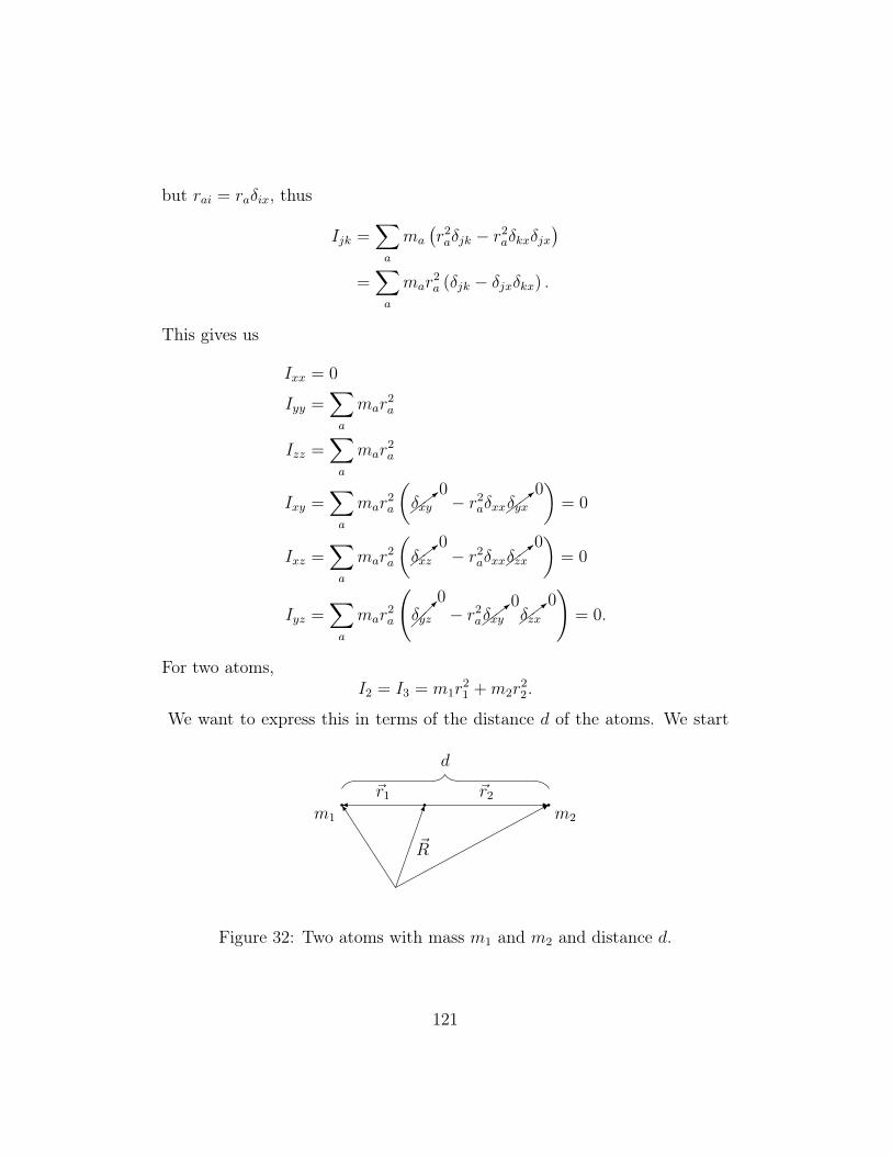
but rai = raδix, thus
Ijk =∑a
ma
(r2aδjk − r2
aδkxδjx)
=∑a
mar2a (δjk − δjxδkx) .
This gives us
Ixx = 0
Iyy =∑a
mar2a
Izz =∑a
mar2a
Ixy =∑a
mar2a
(>
0δxy − r2
aδxx>
0δyx
)= 0
Ixz =∑a
mar2a
(>
0δxz − r2
aδxx>
0δzx
)= 0
Iyz =∑a
mar2a
(
0δyz − r2
a>
0δxy
>0
δzx
)= 0.
For two atoms,I2 = I3 = m1r
21 +m2r
22.
We want to express this in terms of the distance d of the atoms. We start
m2m1
~R
~r1 ~r2
d
Figure 32: Two atoms with mass m1 and m2 and distance d.
121
with the center of mass equation:
0 = m1r1 +m2r2
⇒ r2 = −m1
m2
r1.
We obtain for the distance:
d = r1 − r2
= r1
(1 +
m1
m2
)= r1
m1 +m2
m2
and thus
r1 =m2
m1 +m2
d
r2 = − m1
m1 +m2
d .
Then, the moments of inertia are
I2,3 = m1r21 +m2r
22
=
[m1
(m2
m1 +m2
)2
+m2
(m1
m1 +m2
)2]d2
=m1 +m2
(m1 +m2)2·m1m2
⇒ Iyy = Izz =m1m2
m1 +m2
d2
Now, recallIjk =
∑a
ma
(r2aδjk − rajrak
)and let us shift
ra → ra + c,
thenI ′jk =
∑a
[(ra + c)− (raj + cj)(rak + ck)] .
122
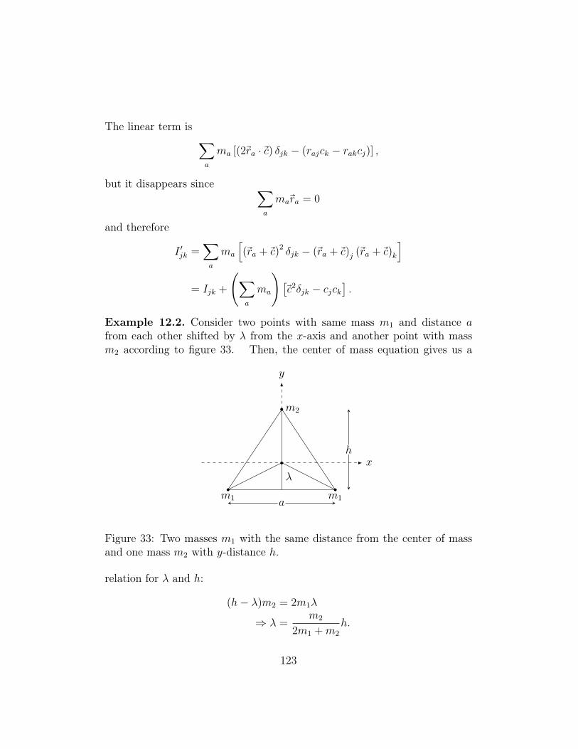
The linear term is ∑a
ma [(2ra · c) δjk − (rajck − rakcj)] ,
but it disappears since ∑a
mara = 0
and therefore
I ′jk =∑a
ma
[(ra + c)2 δjk − (ra + c)j (ra + c)k
]= Ijk +
(∑a
ma
)[c2δjk − cjck
].
Example 12.2. Consider two points with same mass m1 and distance afrom each other shifted by λ from the x-axis and another point with massm2 according to figure 33. Then, the center of mass equation gives us a
x
y
m1 m1
m2
a
h
λ
Figure 33: Two masses m1 with the same distance from the center of massand one mass m2 with y-distance h.
relation for λ and h:
(h− λ)m2 = 2m1λ
⇒ λ =m2
2m1 +m2
h.
123
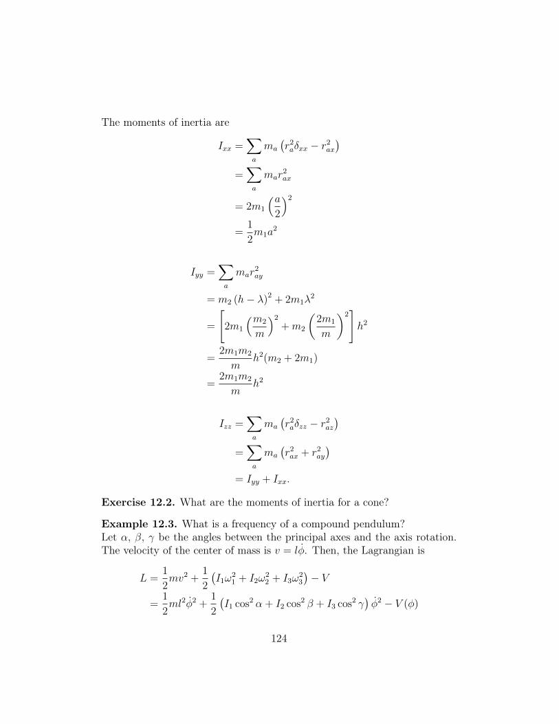
The moments of inertia are
Ixx =∑a
ma
(r2aδxx − r2
ax
)=∑a
mar2ax
= 2m1
(a2
)2
=1
2m1a
2
Iyy =∑a
mar2ay
= m2 (h− λ)2 + 2m1λ2
=
[2m1
(m2
m
)2
+m2
(2m1
m
)2]h2
=2m1m2
mh2(m2 + 2m1)
=2m1m2
mh2
Izz =∑a
ma
(r2aδzz − r2
az
)=∑a
ma
(r2ax + r2
ay
)= Iyy + Ixx.
Exercise 12.2. What are the moments of inertia for a cone?
Example 12.3. What is a frequency of a compound pendulum?Let α, β, γ be the angles between the principal axes and the axis rotation.The velocity of the center of mass is v = lφ. Then, the Lagrangian is
L =1
2mv2 +
1
2
(I1ω
21 + I2ω
22 + I3ω
23
)− V
=1
2ml2φ2 +
1
2
(I1 cos2 α + I2 cos2 β + I3 cos2 γ
)φ2 − V (φ)
124
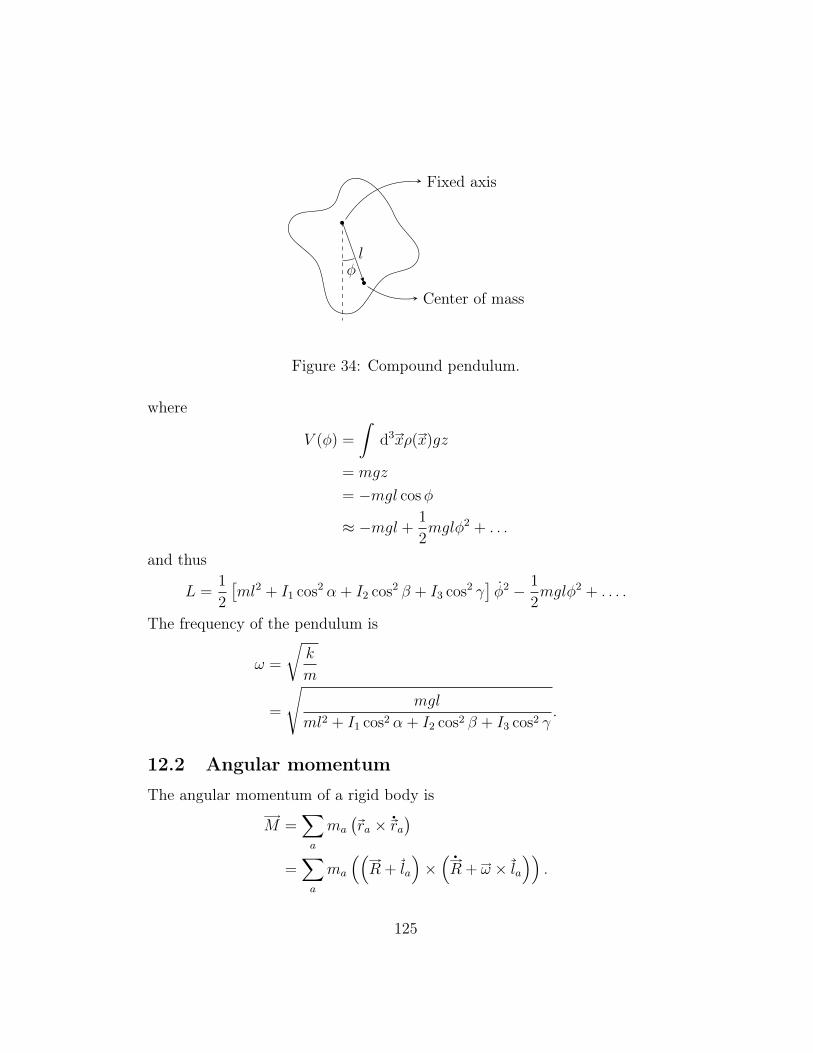
lφ
Fixed axis
Center of mass
Figure 34: Compound pendulum.
where
V (φ) =
∫d3xρ(x)gz
= mgz
= −mgl cosφ
≈ −mgl +1
2mglφ2 + . . .
and thus
L =1
2
[ml2 + I1 cos2 α + I2 cos2 β + I3 cos2 γ
]φ2 − 1
2mglφ2 + . . . .
The frequency of the pendulum is
ω =
√k
m
=
√mgl
ml2 + I1 cos2 α + I2 cos2 β + I3 cos2 γ.
12.2 Angular momentum
The angular momentum of a rigid body is
M =∑a
ma
(ra × ra
)=∑a
ma
((R + la
)×(R + ω × la
)).
125
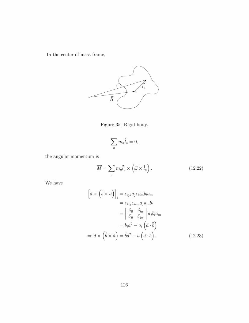
In the center of mass frame,
~la
~R
~r
Figure 35: Rigid body.
∑a
mala = 0,
the angular momentum is
M =∑a
mala ×(ω × la
). (12.22)
We have [a×
(b× a
)]i
= εijkajεklmblam
= εkijεklmajambl
=
∣∣∣∣ δil δinδjl δjn
∣∣∣∣ ajblam= bia
2 − ai(a · b
)⇒ a×
(b× a
)= ba2 − a
(a · b
). (12.23)
126
Thus,
M =∑a
ma
[l2aω − la
(ω · la
)]Mi =
∑a
ma
[l2aωi − lai (lajωj)
]=
(∑a
ma
[l2aδij − lailaj
])ωj
⇒Mi = Iijωj . (12.24)
Changing our axes to the principal axes of inertia, we have
Mi = Iiωi. (12.25)
We observe that the angular momentum is not necessarily aligned to thedirection of the angular velocity. This happens for a spherical top,
I1 = I2 = I3 = I,
for whichM = Iω. (12.26)
12.2.1 Precession
We now examine the motion of a symmetrical top,
I1 = I2 6= I3,
which moves freely, without the influence of external forces. In the center ofmass frame, the motion to the symmetrical top is purely rotational. We candetermine it completely by using angular momentum conservation.One principal axis is the axis of symmetry x3, as shown in Figure 37.
The other two principal axes are perpendicular to it. Due to the symmetry,we have the freedom to choose their orientation. We choose x2-axis to beperpendicular to the plane defined by x3 and the angular momentum M .Then,
M ⊥ x2 ⇒M2 ≡M · x2 = 0,
butM2 = I2ω2 ⇒ ω2 = 0 ,
127
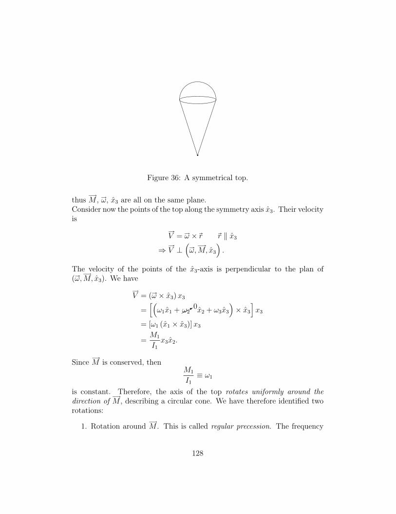
Figure 36: A symmetrical top.
thus M , ω, x3 are all on the same plane.Consider now the points of the top along the symmetry axis x3. Their velocityis
V = ω × r r ‖ x3
⇒ V ⊥(ω,M, x3
).
The velocity of the points of the x3-axis is perpendicular to the plan of(ω,M, x3). We have
V = (ω × x3)x3
=[(ω1x1 +*
0ω2 x2 + ω3x3
)× x3
]x3
= [ω1 (x1 × x3)]x3
=M1
I1
x3x2.
Since M is conserved, thenM1
I1
≡ ω1
is constant. Therefore, the axis of the top rotates uniformly around thedirection of M , describing a circular cone. We have therefore identified tworotations:
1. Rotation around M . This is called regular precession. The frequency
128
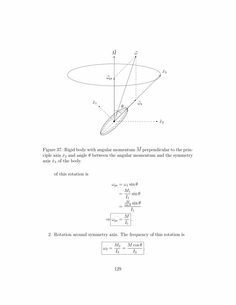
~M
x3
x1
~ω
~ω3
~ωpr
θ
x2
Figure 37: Rigid body with angular momentumM perpendicular to the prin-ciple axis x2 and angle θ between the angular momentum and the symmetryaxis x3 of the body.
of this rotation is
ωpr = ω1 sin θ
=M1
I1
sin θ
=M
sin θsin θ
I1
⇒ ωpr =M
I1
.
2. Rotation around symmetry axis. The frequency of this rotation is
ω3 =M3
I3
=M cos θ
I3
.
129
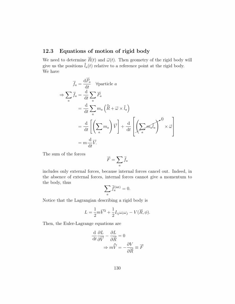
12.3 Equations of motion of rigid body
We need to determine R(t) and ω(t). Then geometry of the rigid body willgive us the positions la(t) relative to a reference point at the rigid body.We have
fa =dPadt
∀particle a
⇒∑a
fa =d
dt
∑a
Pa
=d
dt
∑a
ma
(R + ω × la
)
=d
dt
[(∑a
ma
)V
]+
d
dt
*0(∑
a
mala
)× ω
= m
d
dtV.
The sum of the forcesF =
∑a
fa
includes only external forces, because internal forces cancel out. Indeed, inthe absence of external forces, internal forces cannot give a momentum tothe body, thus ∑
a
f (int)a = 0.
Notice that the Lagrangian describing a rigid body is
L =1
2mV 2 +
1
2Iijωiωj − V (R, φ).
Then, the Euler-Lagrange equations are
d
dt
∂L
∂V− ∂L
∂R= 0
⇒ mV = −∂V∂R≡ F
130
where we have used the shorthand notation∂
∂x= ∇
x≡(
∂
∂x1
,∂
∂x2
,∂
∂x3
).
Now let us look at the rate of change of the total angular momentum. Let usspecify the reference frame to be so that the center of mass does not move:
V = 0.
This is not necessarily an inertial frame.Then,
dM
dt=
d
dt
(∑a
la × Pa
)
=∑a
d
dtla × Pa +
∑a
la ×dPadt
=∑a
:0d
dtla ×
(ma
dladt
)+∑a
la ×dPadt
=∑a
la × fa.
The sumK ≡
∑a
la × fa
is the total torque. The above sum includes only external forces, since theinternal forces alone cannot produce angular momentum.
dM
dt= K
can be derived from the Lagrangian:d
dt
∂L
∂ω− ∂L
∂φ= 0,
where
∂L
∂ωi=
∂
∂ωi
(1
2ωi∑j
Iijωj
)=∑j
Iijωj = Mi
∂L
∂φi= −∂V
∂φi.
131
For
∂V = −∑a
fa · ∂la︸ ︷︷ ︸work
= −∑a
fa ·(∂φ× la
)= −∂φ ·
∑a
(la × fa
)︸ ︷︷ ︸
=K
= −∂φ ·K,we obtain
−∂V∂φ
= K.
The equations of motion
dP
dt= F (total force)
dM
dt= K (total torque)
have been derived for a reference frame where the axes have a fixed orienta-tion.However, it is often convenient to use a reference frame with rotating axes.Typically, these are the principal axes of inertia. Consider two coordinatesystems where (x1, x2, x3) are fixed and (y1(t), y2(t), y3(t)) are rotating.If we express a vector A in terms of the rotating system, we have
A =∑i
Aiyi(t).
The total derivative isdA
dt=∑i
dAidt
yi(t) +∑i
Ai(t)dyi(t)
dt
=∑i
dAidt
yi(t) +∑i
Ai(t)ω × yi(t)
⇒ dA
dt=
(dA
dt
)rot
+ ω × A . (12.27)
132
In (12.27),
(dA
dt
)rot
is the rate of change of the vector A as it is perceived
in the rotating frame.
Therefore, in a rotating reference frame with a fixed (or freely moving)center the equations of motion take the form(
dP
dt
)rot
+ ω × P = F(dM
dt
)rot
+ ω ×M = K
where ω is the angular velocity vector for the rotation of the rotating frame.In terms of components, we have
m
(dV1
dt+ ω2v3 − ω3v2
)= F1
m
(dV2
dt+ ω3v1 − ω1v3
)= F2
m
(dV3
dt+ ω1v2 − ω2v1
)= F3.
We can choose the axes of the rotating system to be the principal axes ofinertia. Then, using
M1 = I1ω1 M2 = I2ω2 M3 = I3ω3
and substituting into (dM
dt
)rot
+ ω ×M = K,
we have
I1dω1
dt+ (I3 − I1)ω2ω3 = K1
I1dω2
dt+ (I1 − I3)ω3ω1 = K2
I1dω3
dt+ (I2 − I1)ω1ω2 = K3.
Euler’s equations
133
12.3.1 Applications: Free rotational motion
Example 12.4 (Symmetrical top). In this case, we have
I1 = I2 6= I3 K = 0
and fordω3
dt= 0 ⇒ ω3 = const,
we obtain
dω1
dt+ Ωω2 = 0 (12.28)
dω2
dt− Ωω1 = 0 (12.29)
withΩ ≡ ω3
I3 − I1
I1
.
This leads to
ω1 = −Ωω2
ω2 = Ωω1
and we can decouple this system of differential equations:
d
dt(ω1 + iω2) = Ω(−ω2 + iω1)
= iΩ(ω1 + iω2)
⇒ ω1 + iω2 = AeiΩt
= A(cosωt+ i sinωt)
⇒ ω1 = A cosωt ω2 = A sinωt .
Notice that
ω21 + ω2
2 + ω23 = A2 + ω2
3 = const. ⇒ |ω| = const.,
i.e. the magnitude of the angular velocity is constant.Since ω3 is constant too, then ω rotates around the symmetry axis of the topwith angular velocity Ω.
134
Example 12.5 (Asymmetrical top). Let us now consider the general case ofan asymmetric top:
I3 > I2 > I1.
Energy and angular momentum conservation give
1
2I1ω
21 +
1
2I2ω
22 +
1
2I3ω
23 = E
⇒ M21
I1
+M2
2
I2
+M2
3
I3
= 2E
andM2
1 +M22 +M2
3 = M2.
This is the intersection of a sphere and an ellipsoid.We can prove easily the inequalities
2EI1 ≤M2 ≤ 2EI3 .
If M2 = 2EI1 (smallest value),
M2 = M3 = 0.
For M2 = 2EI3,
M21
I1
+M2
2
I2
+M2
3
I3
= 2E
M21 +M2
2 +M23 = M2.
For M2 = 2EI2,
M21
I1
+M2
2
I2
+M2
3
I3
= 2E
M21
I2
+M2
2
I2
+M2
3
I2
= 2E
⇒M21
(1
I1
− 1
I2
)+M2
3
(1
I3
− 1
I2
)= 0
⇒M21 = M2
3 .
135
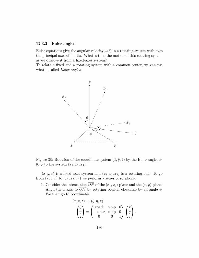
12.3.2 Euler angles
Euler equations give the angular velocity ω(t) in a rotating system with axesthe principal axes of inertia. What is then the motion of this rotating systemas we observe it from a fixed-axes system?To relate a fixed and a rotating system with a common center, we can usewhat is called Euler angles.
x
y
z
x1
x2
x3
ξ
φ
ψ
θ
Figure 38: Rotation of the coordinate system (x, y, z) by the Euler angles φ,θ, ψ to the system (x1, x2, x3).
(x, y, z) is a fixed axes system and (x1, x2, x3) is a rotating one. To gofrom (x, y, z) to (x1, x2, x3) we perform a series of rotations.
1. Consider the intersection ON of the (x1, x2)-plane and the (x, y)-plane.Align the x-axis to ON by rotating counter-clockwise by an angle φ.We then go to coordinates
(x, y, z)→ (ξ, η, z)ξηz
=
cosφ sinφ 0− sinφ cosφ 0
0 0 1
xyz
.
136
2. Then we rotate around the ξ(≡ ON)-axis counter-clockwise: ξη′
z′
=
1 0 00 cos θ sin θ0 − sin θ cos θ
ξηz
.
3. Finally, we rotate around the z′-axis by ψ:x1
x2
x3
=
cosψ sinψ 0− sinψ cosψ 0
0 0 1
ξη′
z′
.
Collectively, we can write:x1
x2
x3
=
cosψ sinψ 0− sinψ cosψ 0
0 0 1
1 0 00 cos θ sin θ0 − sin θ cos θ
cosφ sinφ 0− sinφ cosφ 0
0 0 1
xyz
.
We can now relate the angular velocity
ω = (θ1, θ2, θ3)
as seen in the (x1, x2, x3)-frame in terms of the Euler angles and angularvelocities.For the Euler angular velocities we have:
φ = φz
θ = θξ
ψ = ψz′.
We want to express these rotation axes in terms of x1, x2 and x3:
ξ = (ξ · x1) · x1 + (ξ · x2) · x2 +*
0(ξ · x3) · x3
= cosψx1 + cos(ψ +
π
2
)x2
= cosψx1 − sinψx2
137
z = cos θx3 + sin θ cos(π
2− ψ
)x1 + sin θ cosψx2
= cos θx3 + sin θ sinψx1 + sin θ cosψx2
z′ = x3,
then
ω = θ + φ+ ψ
= (φ sin θ sinψ + θ cosψ)x1 + (ψ sin θ cosψ − θ sinψ)x2 + (φ cos θ + ψ)x3.
138
13 Hamiltonian mechanicsAs we established in Sect. 4.6, the motion of a holonomic system with ndegrees of freedom is determined by the Lagrange equations, that is a setof n second order differential equations in n unknown variables qi, where wespecify the initial conditions given by qi and qi at a given time t.
It has been known since Lagrange’s times that higher order differentialequations can be reduced to systems of first order differential equations.Thus, we expect that a system of n second order differential equations canbe reduced to a system of 2n first order differential equations. In general, itis more convenient to deal with a system of first order differential equations,because an approximate solution may be found even when an exact solutionis not known. To illustrate this point, let us consider a point whose motionis described by the first order differential equation,
r(t) = f (r(t); t) . (13.1)
Given an initial condition at a time t0, eq. (13.1) can be integrated to,
r(t) = r(t0) +
∫ t
t0
f (r(τ); τ) dτ . (13.2)
The integral equation (13.2) is more convenient than the differential one(13.1) because it can be approximated. In fact, given the initial conditionr(t0), we can build a series of successive approximations through the iterativeformula,
rk+1(t) = r(t0) +
∫ t
t0
f (rk(τ); τ) dτ , k = 0, 1, 2, . . . . (13.3)
For example, let us take the non-linear differential equation in one dimension,
x(t) = x2 + t2 , (13.4)
with t0 = 0 and initial condition x(t0) = x0(t) = 0. Then,
x1(t) =
∫ t
0
[x2
0(τ) + τ 2]
dτ =
∫ t
0
τ 2dτ =t3
3,
x2(t) =
∫ t
0
[x2
1(τ) + τ 2]
dτ =
∫ t
0
(τ 6
9+ τ 2
)dτ =
t3
3+t7
63, (13.5)
139
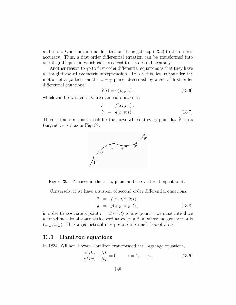
and so on. One can continue like this until one gets eq. (13.2) to the desiredaccuracy. Thus, a first order differential equation can be transformed intoan integral equation which can be solved to the desired accuracy.
Another reason to go to first order differential equations is that they havea straightforward geometric interpretation. To see this, let us consider themotion of a particle on the x − y plane, described by a set of first orderdifferential equations,
r(t) = v(x, y; t) , (13.6)which can be written in Cartesian coordinates as,
x = f(x, y; t) ,
y = g(x, y; t) . (13.7)
Then to find r means to look for the curve which at every point has r as itstangent vector, as in Fig. 39.
Figure 39: A curve in the x− y plane and the vectors tangent to it.
Conversely, if we have a system of second order differential equations,
x = f(x, y, x, y; t) ,
y = g(x, y, x, y; t) , (13.8)
in order to associate a point r = a(r, r; t) to any point r, we must introducea four-dimensional space with coordinates (x, y, x, y) whose tangent vector is(x, y, x, y). Thus a geometrical interpretation is much less obvious.
13.1 Hamilton equations
In 1834, William Rowan Hamilton transformed the Lagrange equations,d
dt
∂L
∂qi− ∂L
∂qi= 0 , i = 1, . . . , n , (13.9)
140
into a system of 2n first order differential equations. To do so, he introducedthe conjugate momenta pi to the generalized coordinates qi,
pi =∂L
∂qi, i = 1, . . . , n , (13.10)
and proposed to use qi, pi and t as the canonical variables, rather than thevariables qi, qi and t used by Lagrange. If the Jacobian of pi in eq. (13.10) isnon-vanishing, ∣∣∣∣∂pi∂qj
∣∣∣∣ =
∣∣∣∣ ∂2L
∂qi∂qj
∣∣∣∣ 6= 0 , (13.11)
then we can invert eq. (13.10), and write that
qi = qi(qk, pk, t) , (13.12)
that is, we can express the Lagrange variables in terms of Hamilton variablesand viceversa. In particular, for natural systems, for which the Lagrangianis a quadratic function of the generalized velocities, eq. (13.10) expresses alinear relation between conjugate momenta and generalized velocities.
Hamilton introduced a functionH(qk, pk, t), called theHamiltonian, whichis defined through the Legendre transformation,
H =n∑i=1
piqi − L , (13.13)
and showed that one can transform the Lagrange equations into a system offirst order differential equations,
qi =∂H
∂pi, pi = −∂H
∂qi, i = 1, . . . , n , (13.14)
which are called the Hamilton equations.In order to prove Hamilton equations, we shall use Donkin’s theorem,
which states that given a function of n variables, X(x1, . . . , xn), with a non-vanishing Hessian, ∣∣∣∣ ∂2X
∂xi∂xj
∣∣∣∣ 6= 0 , (13.15)
and given a set of auxiliary variables,
yi =∂X
∂xi, i = 1, . . . , n , (13.16)
141
there is a transformation which is the inverse of eq. (13.16) and is generatedby a function Y (y1, . . . , yn), such that,
xi =∂Y
∂yi, i = 1, . . . , n . (13.17)
The function Y generating the inverse transformation is related to the func-tion X by the Legendre transformation,
Y =n∑i=1
xiyi −X . (13.18)
Furthermore, ifX depends onmmore variables,X = X(x1, . . . , xn;α1, . . . , αm),then also Y depends on m more variables, Y = Y (y1, . . . , yn;α1, . . . , αm),with the relation,
∂X
∂αk= − ∂Y
∂αk, k = 1, . . . ,m . (13.19)
Proof of Donkin’s theorem. Because the Hessian of X, which is the Jaco-bian of yi is non-vanishing,∣∣∣∣ ∂2X
∂xi∂xj
∣∣∣∣ =
∣∣∣∣ ∂yi∂xj
∣∣∣∣ 6= 0 , (13.20)
eq. (13.16) can be inverted, and we can write xi = xi(y1, . . . , yn). Let us takea function Y (y1, . . . , yn) to be given by a Legendre transformation (13.18).Then,
∂Y
∂yi=
∂
∂yi
(n∑k=1
xkyk −X
)
=∂xk∂yi
yk + xi −∂X
∂yi
=∂xk∂yi
yk + xi −∑k
∂X
∂xk
∂xk∂yi
= xi , (13.21)
where in the last step above we used the chain rule and eq. (13.16).
142
If X depends on m more variables, X = X(x1, . . . , xn;α1, . . . , αm), thosevariables appear in eq. (13.16) and in the inverse transformation as well,
xi = xi(y1, . . . , yn;α1, . . . , αm) . (13.22)
The function Y is given by the Legendre transformation (13.18) with thevariables xi given by the inverse transformation (13.22),
∂Y
∂αi
∣∣∣∣yj
=∂
∂αi
(n∑k=1
xkyk −X
)
=∑k
∂xk∂αi
yk −∑k
∂X
∂xk
∂xk∂αi− ∂X
∂αi
= −∂X∂αi
, (13.23)
which completes the proof of Donkin’s theorem.In order to obtain Hamilton equations, we identify,
X ≡ L ,
xi ≡ qi ,
yi ≡ pi ,
αi ≡ qi, t , (13.24)
with i = 1, . . . , n. Then Donkin’s theorem implies that given a functionL(q1, . . . , qn; q1, . . . , qn; t), and a set of auxiliary variables (13.10), there is afunction H(q1, . . . , qn; p1, . . . , pn; t) which generates the inverse transforma-tion of eq. (13.10),
qi =∂H
∂pi, i = 1, . . . , n . (13.25)
The Hamiltonian H is related to the Lagrangian L by the Legendre trans-formation (13.18),
H =n∑i=1
piqi − L , (13.26)
with∂L
∂qi= −∂H
∂qi,
∂L
∂t= −∂H
∂t. (13.27)
143
Lagrange equations (13.9) and eq. (13.10) imply that,
pi =∂L
∂qi, (13.28)
and using eq. (13.27), we get that,
pi = −∂H∂qi
. (13.29)
Eqs. (13.25) and (13.29) form a system of 2n first order differential equations,the Hamilton equations (13.14).
Hamilton equations imply that the total time derivative of the Hamilto-nian H equals the partial time derivative,
dH
dt=∑i
(∂H
∂pipi +
∂H
∂qiqi
)+∂H
∂t=∂H
∂t. (13.30)
From eq. (7.1) and from the Legendre transformation (13.13), we realizethat for a conservative system the Hamiltonian is the total energy of thesystem. But for a conservative system the total energy is conserved, so
dH
dt=∂H
∂t= 0 , (13.31)
that is, the HamiltonianH = H(q1, . . . , qn; p1, . . . , pn) is a constant of motion.For elementary systems, solving a system of Hamilton equations is not
usually simpler than solving the analogous system of Lagrange equations.However, the strength of the Hamilton equations may be appreciated whendealing with complex dynamic systems, like the planetary orbits in celestialmechanics, which can be treated through approximate methods of perturba-tion theory using Hamiltonian mechanics. Furthermore, Hamilton equationsnaturally incorporate the concept of symmetry: if a coordinate q is associatedto a symmetry, its conjugate momentum p is conserved and the Hamiltoniandoes not depend on q, effectively reducing the system to n−1 variables. Thatis not apparent with Lagrange equations, which in that case will still dependon n velocities qi. Also, although Hamilton equations cannot be used as suchin quantum mechanics, their structure inspires the equations of quantum me-chanics. Finally, Hamiltonian mechanics has a natural geometric structure interms of simplectic manifolds (to be defined later). In the following lectures,we will briefly explore some of the benefits of Hamiltonian mechanics listedabove.
144
13.2 The Hamiltonian as a conserved quantity and/orthe total energy
The simplest Hamiltonian we can consider is for a particle moving on a planexy under the action of a central potential. The Lagrangian is
L =m
2
(x2 + y2
)− V (x, y).
The conjugate momenta are
px =∂L
∂x= mx
py =∂L
∂y= my
which we invert tox =
pxm
y =pym
such that the Lagrangian becomes
L =1
2m
(p2x + p2
y
)− V (x, y).
The Hamiltonian is
H = pxx+ pyy − L
=1
m
(p2x + p2
y
)− 1
2m
(p2x + p2
y
)+ V (x, y)
=1
2m
(p2x + p2
y
)+ V (x, y).
Note that the Hamiltonian is the total energy of the particle, and it is also aconserved quantity, since
∂L
∂t= −∂H
∂t= 0.
Let us examine these concept more in detail. We said that for a conserva-tive system, the kinetic and potential energies do not depend on time. Thenthe Lagrangian does not either,
∂L
∂t= 0,
145
and thus ∑i
∂L
∂qiqi − L
is a conserved quantity which we identify with the Hamiltonian
H =∑i
piqi − L.
We just saw that for a particle in central potential, H is also the total energyE, and that is true in fact for any conservative system.
In the tutorials, we showed that for a conservative system, defined as aholonomic system with:
• only stationary contraints,
• the potential energy which does not depend explicitly on time,
• no non-potential forces
the total energy is conserved:
dE
dt= 0.
Let us examine the concepts of total energy and conserved quantity in theHamiltonian language. We know that if
∂L
∂t= −∂H
∂t= 0,
H is a conserved quantity. Under what conditions is H the total energy ofthe system?
In the Lagrangian formalism, we established that for a holonomic system,the Euler-Lagrange equations are
d
dt
∂L
∂qi− ∂L
∂qi= Qi
with L = T − V and the non-potential force Qi(qj, qj, t).Let us suppose that the non-potential force Qi (called so because it does not
146
come from an ordinary potential V (qi, t)) comes actually from a generalizedpotential V (qi, qi, t), through the equation
Qi =d
dt
∂V
∂qi− ∂V
∂qi(13.32)
then we can still write the Euler-Lagrange equations as
d
dt
∂L
∂qi− ∂L
∂qi= 0
if we require that L = T − V . Then (13.32) implies that
Qi =∑n
∂2V
∂qi∂qnqn + . . . .
However, in the generalized force there is no explicit dependence on acceler-ations qn, since
Qi = Qi(qn, qn, t).
Thus∂2V
∂qi∂qn= 0,
so the potential V can be at most linear in the velocities:
V =∑i
aiqi + U
= V1 + U
where U is the ordinary potential.We have already seen an example of such a potential: a particle in an elec-tromagnetic field has potential
V = eφ− e
cr · A.
Next, we restrict ourselves to “natural” systems, i.e. systems for whichthe kinetic energy, and thus the Lagrangian, are at most quadratic in thevelocities (so far we have only met “natural” systems, but there is an im-portant “non-natural” system: a relativistic particle). However, apart from
147
this restriction, the following discussion is general. The kinetic energy of anatural system is
T = T2 + T1 + T0
withT2 =
∑i,n
ainqiqn T1 =∑i
biqi
and the Lagrangian is
L = T − V = L2 + L1 + L0
withL2 = T2 L1 = T1 − V1 L0 = T0 − U.
The Hamiltonian is
H =∑i
piqi − L =∑i
∂L
∂qiqi − L.
Then we use Euler’s theorem on homogeneous functions,∑i
∂L2
∂qiqi = 2L2
∑i
∂L1
∂qiqi = L1,
thus
H = 2L2 + L1 − (L2 + L1 + L0)
= L2 − L0
which is independent of whether a potential dependent on velocities is presentor not. In particular,
H = T2 − T0 + U .
As we saw on the tutorial on the energy of a holonomic system, for a systemwith constraints which do not depend explicitly on time, T0 = 0, T = T2,then
H = T + U .
Thus we have established that the most general condition for a natural systemto have the Hamiltonian as the total energy is that the constraints do notdepend explicitly on time.
148
Example 13.1. For a particle in an electromagnetic field, the Lagrangian is
L =mr2
2− eφ+
e
cr · A.
The conjugate momenta are
px =∂L
∂x= mx+
e
cAx and likewise for y,z.
The Hamiltonian is
H = pxx+ pyy + pz z − L
=mr2
2+ eφ
=1
2m
(p− e
cA)2
+ eφ
i.e. the total energy of the particle.
Now, the difference between the Hamiltonian being a conserved quantityor the total energy is clear:A system might have the Hamiltonian
H = H(qi, pi)
which does not depend explicitly on time, then
∂H
∂t= 0
and H is a conserved quantity. However, the constraints might be non-stationary,
rm = rm(q1, . . . , qm, t),
thenH = T2 − T0 + U
is not the total energy.
149
13.3 Cyclic coordinates
When studying conservation laws, we saw that if a coordinate qn is cyclic,i.e. such that
∂L
∂qn= 0
the Euler-Lagrange equations imply that
d
dt
∂L
∂qn= 0.
Becuase the conjugate momentum is
pn =∂L
∂qn
that means that pn is conserved pn = cn.
In the Hamiltonian formalism, this means that H depends on 2(n − 1)variables and a constant cn, to be fixed by the initial conditions
H = H(q1, . . . , qn−1; p1, . . . , pn−1; cn; t)
since qn does not occur in the Legendre transform
H =∑i
piqi − L(q1, . . . , qn−1; q1, . . . , qn; t)
andpn = −∂H
∂qn= 0 ⇒ pn = cn.
Effectively, the system has gone from n to n− 1 degrees of freedom (DOF).In contrast, in the Lagrangian formalism the system still depends on n DOF:
L = L(q1, . . . , qn−1; q1, . . . , qn; t).
So a Hamiltonian formulation is particularly convenient when cyclic coordi-nates are present.
Example 13.2. The motion of a particle in a central potential V (r) in polarcoordinates r, θ.
150
The Lagrangian is
L =m
2
(r2 + r2θ2
)− V (r).
Because the system is conservative, the Hamiltonian is
H = T + V (r).
The conjugate momenta are
pr =∂L
∂r= mr
pθ =∂L
∂θ= mr2θ
which can be inverted,r =
prm
θ =pθmr2
.
Thus, the Hamiltonian is
H =1
2m
(p2r +
p2θ
r2
)+ V (r).
The Hamiltonian equations are
r =∂H
∂pr=prm
θ =∂H
∂pθ=
pθmr2
pr = −∂H∂r
=p2θ
mr3− ∂V
∂ri.e. the equation of the force in a central potential
pθ = −∂H∂θ
= 0 angular momentum conservation.
Note that θ is cyclic and pθ = M is is conserved. The Hamiltonian dependson one DOF and one constant, the angular momentum M :
H = H(r; pr;M).
151
13.4 Hamilton’s equations and Hamilton’s principle
Hamilton’s principle was to require the action
S =
∫ tf
ti
dt L [qj(t) , qj(t) ; t]
to be minimal:δS = 0
where qi is a short-hand for q1, . . . , qn.In the Hamiltonian formulation, we require that
δS = δ
∫ tf
ti
dt
(∑i
piqi −H [pj , qj , t]
)= 0
is minimal on the 4n-dimensional phase space which depends on the coordi-nates q and p, and their time derivatives q and p.It is like in variational calculus: we must minimize the integral
I [q , p] =
∫ tf
ti
dt f (q , p , q , p , t)
where f =∑i
piqi −H.
Then δI = 0 leads to the Euler-Lagrange equations
d
dt
∂f
∂qi− ∂f
∂qi= 0 (13.33)
d
dt
∂f
∂pi− ∂f
∂pi= 0 (13.34)
which, for f as given above, yield:
(13.33) ⇒ pi +∂H
∂qi= 0
(13.34) ⇒ −qi +∂H
∂pi= 0.
So, in a very concise way, we obtained Hamilton’s equations!
152
13.5 Canonical transformations
The motion of a particle in a plane under the action of a central potential canbe described using Cartesian coordinates x, y or polar coordinates r, θ as gen-eralized coordinates. The advantage with polar coordinates is that θ is cyclic.
In general, given a Hamiltonian
H(q1, . . . , qn; p1, . . . , pn; t)
the coordinates q1, . . . , qn might not be cyclic, but there might be anotherset of coordinates Q1, . . . , Qn for which some or all of them are cyclic.It is important then to have a procedure to go from one set (q , p)in the2n-dimensional space to another:
Qi = Qi (q ; p ; t)
Pi = Pi (q ; p ; t) .
The coordinates Qi, Pi must also be canonical, i.e. there must be a function
K(Q1, . . . , Qn;P1, . . . , Pn; t)
such thatQi =
∂K
∂PiPi = − ∂K
∂Qi
.
So they must satisfy Hamilton’s principle
δ
∫ tf
ti
dt
(∑i
PiQi −K (Q ; P ; t)
)= 0
just like for the old coordinates
δ
∫ tf
ti
dt
(∑i
piqi −H (q ; p ; t)
)= 0.
Then the two integrands must be the same, up to a variation on the endpoints, whose integral vanishes:∑
i
piqi −H =∑i
PiQi −K +dF
dt(13.35)
153
where F cannot be a function of the phase space coordinates (q , p)or (Q , P) since they have null variation on the end points, but it canbe a function of a mixture of old and new variables, for example F =F (q , Q ; t). Then (13.35) implies that∑
i
piqi −H =∑i
PiQi −K +∑i
(∂F
∂qiqi +
∂F
∂Qi
Qi
)+∂F
∂t.
Since qi andQi are independent, so are their time derivatives qi and Qi, whosecoefficients must vanish. Thus, we obtain the transformation equations:
pi =∂F
∂qiPi = − ∂F
∂Qi
andK = H +
∂F
∂t.
The function F is called the generating function of the canonical transfor-mation above. If we set in particular,
F (q , Q) =n∑k=1
qkQk,
then the transformation equations are
pi =∂F
∂qi= Qi
Pi = − ∂F∂Qi
= −qi
i.e. this canonical transformation interchanges momenta and coordinates. Inthe Hamiltonian formalism momenta and space coordinates are coordinateson an equal footing of the 2n-dimensional phase space. There is no memoryof q being a space coordinate and p a mass times a velocity.
If pi cannot be taken as a function of qj and Qj, it is suitable to take afunction of the type F = F (q , P ; t) as a generating function. But sincein eq. (13.35), Pi does not occur, it is more convenient to set
F = G (q , P ; t)−∑k
QkPk
154
such that eq. (13.35) becomes∑i
piqi −H = −∑i
QiPi −K +dG
dt(13.36)
Making the total derivative explicit,∑i
piqi −H = −∑i
QiPi −K +∑i
(∂G
∂qiqi +
∂G
∂PiPi
)+∂G
∂t,
and considering that qi and Pi are independent, we obtain the transformationequations:
pi =∂G
∂qiQi =
∂G
∂Piand
K = H +∂G
∂t.
Note that if we take in particular,
G (q , P) =n∑k=1
qkPk, (13.37)
then the transformation equations are
pi =∂G
∂qi= Pi
Qi =∂G
∂Pi= qi
andK = H,
i.e. the new coordinated equal the old ones: the function (13.37) generatesthe identity transformation.
One can also consider
F = F (p , Q , t)F = F (p , P , t)
as generating functions (a classification of, and relations among, the F ’s isgiven in Goldstein’s book), and any combinations of them. The classifica-tion above is not exhaustive: there might be generating functions which donot conform to any of the types given above.
155
13.6 A canonical transformation for the harmonic oscil-lator
Consider a harmonic oscillator in one dimension, with force constant k. TheHamiltonian is
H =p2
2m+kq2
2=
1
2m
(p2 +m2ω2q2
)where one can set k = mω2 with ω the angular frequency of the oscillation.Because H is a sum of two squares, if we find a canonical transformation
p = f(P ) cosQ
q =f(P )
mωsinQ
(13.38)
then
K = H =f 2(P )
2m
(cos2Q+ sin2Q
)=f 2(P )
2m
so that Q is cyclic. We must find a function f(P ) which makes the transfor-mation canonical.As a generating function, we try
F =mωq2
2cotQ,
then the transformation equations are
p =∂F
∂q= mωq cotQ
P = −∂F∂Q
= −mωq2
2
(−1− cos2Q
sin2Q
)=
mωq2
2 sin2Q
which we can solve for q and p:
p =√
2mωP cosQ
q =
√2P
mωsinQ.
156
Comparing to (13.38), we see that the transformation is canonical if we choose
f(P ) =√
2mωP.
Then the Hamiltonian is
H =2mωP
2m= ωP.
The harmonic oscillator is a conservative system, thus the Hamiltonian isthe total energy. Since the Hamiltonian is cyclic in Q, the momentum P isconstant:
P =E
ω.
Hamilton’s equation for Q is
Q =∂H
∂P= ω
which is trivially integrated:
Q(t) = ωt+ α.
Returning then to the original variables gives us
q(t) =
√2E
mω2sin(ωt+ α)
p(t) =√
2mE cos(ωt+ α).
Accordingly, also the phase space plots look different for the old q, p and thenew Q,P variables. Since
q2
2Emω2
+p2
2mE= 1
the (q, p) plot is an ellipse with
major semi-axis A =
√2E
mω2
minor semi-axis B =√
2mE
and the (Q,P ) plot is a straight line.
157
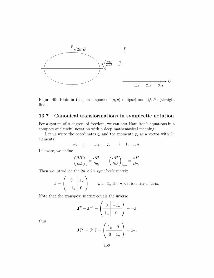
q
p
√2Emω2
√2mE
Q
P
1ωt 2ωt 3ωt
Eω
Figure 40: Plots in the phase space of (q, p) (ellipse) and (Q,P ) (straightline).
13.7 Canonical transformations in symplectic notation
For a system of n degrees of freedom, we can cast Hamilton’s equations in acompact and useful notation with a deep mathematical meaning.
Let us write the coordinates qi and the momenta pi as a vector with 2nelements:
ωi = qi ωi+n = pi i = 1, . . . , n.
Likewise, we define(∂H
∂ω
)i
=∂H
∂qi
(∂H
∂ω
)i+n
=∂H
∂pi.
Then we introduce the 2n× 2n symplectic matrix
J =
0 1n
−1n 0
with 1n the n× n identity matrix.
Note that the transpose matrix equals the inverse
JT = J−1 =
0 −1n1n 0
= −J
thus
JJT = JTJ =
1n 0
0 1n
= 12n
158
andJ2 = −12n.
Then Hamilton’s equations can be written as
ω = J∂H
∂ω
or in components: qi
pi
=
0 1n
−1n 0
∂H
∂qi∂H
∂pi
⇒
qi =
∂H
∂pi
pi = −∂H∂qi
.
Now let us consider a restricted canonical transformation (i.e. one withno explicit dependence on time):
Qi = Qi (q , p)Pi = Pi (q , p) .
(13.39)
Because there is no dependence on time, the new Hamiltonian will equal theold one,
K = H.
The time derivative of Qi is
Qi =∑j
(∂Qi
∂qjqj +
∂Qi
∂pjpj
)=∑j
(∂Qi
∂qj
∂H
∂pj− ∂Qi
∂pj
∂H
∂qj
). (13.40)
We can also invert (13.39),
qi = qi (Q , P)pi = pi (Q , P)
and write the Hamiltonian as a function of Q and P . Thus, we can write
∂H
∂Pi=∑j
[∂H
∂qj
∂qj∂Pi
+∂H
∂pj
∂pj∂Pi
]
159
and equating it to (13.40), we obtain(∂Qi
∂qj
)q,p
=
(∂pj∂Pi
)Q,P
(∂Qi
∂pj
)q,p
= −(∂qj∂Pi
)Q,P
(13.41)
where the indices remind us that on the l.h.s. of the equations Qi is a functionof q, p and on the r.h.s. pj is a function of Q,P .
A comparison of Pi with∂H
∂Qi
yields
(∂Pi∂qj
)q,p
= −(∂pj∂Qi
)Q,P
(∂Pi∂pj
)q,p
=
(∂qj∂Qi
)Q,P
. (13.42)
Eqs. (13.41) and (13.42) characterize a (restricted) canonical transformation,and are equivalent to the method of the generating function introduced be-fore. Thus, a canonical transformation can be obtained finding a suitablegenerating function or through eqs. (13.41) and (13.42). Although the pro-cedure above has been displayed for restricted canonical transformations itis not less general, because it can be extended to canonical transformationsin general.
Remembering that in symplectic notation, Hamilton’s equations are
ω = J∂H
∂ωwith J =
0 1
−1 0
.
The restricted canonical transformation can be written as
Ω = Ω(ω).
Then, taking the time derivative
Ω = Mω
or, in components,
Ωi =∂Ωi
∂ωjωj with Mij =
∂Ωi
∂ωj.
160
Using Hamilton’s equations, we write
Ω = MJ∂H
∂ω.
By the inverse transformation, we can see H as a function of Ωi and write
∂H
∂ωi=∂H
∂Ωj
∂Ωj
∂ωior
∂H
∂ω= MT ∂H
∂Ω,
thenΩ = MJMT ∂H
∂Ω. (13.43)
But the Hamiltonian is the same in the old and the new variables, andHamilton’s equations do not change form, so
Ω = J∂H
∂Ω
and equating with (13.43), we obtain the condition
MJMT = J
which defines the symplectic matrices, and is called the symplectic conditionfor a canonical transformation.
13.8 Infinitesimal canonical transformations
The canonical transformation
Ω = Ω (ω, t)
withωi = qi ωi+n = pi Ωi = Qi Ωi+n = Pi
changes continuously with time.If the transformation ω → Ω (t) is canonical, so is the transformation ω →Ω (t0), thus Ω (t0)→ Ω (t) should be canonical as well.To show that, let us consider an infinitesimal canonical transformation (ICT)
Ω = ω + δω,
161
or in components,Qi = qi + δqi Pi = pi + δpi.
Let us take a generating function of type
G (q , P , t)
as a continuous deformation of the identity transformation:
G =∑k
qkPk + εG (q , P , t) with ε 1.
Then, the transformation equations are
pi =∂G
∂qi= Pi + ε
∂G
∂qi
Qi =∂G
∂Pi= qi + ε
∂G
∂Pi
so the deformations of the canonical variables are
δpi = Pi − pi = −ε∂G∂qi
δqi = Qi − qi = ε∂G
∂Pi= ε
∂G
∂pi
where in the equation for δqi we replaced Pi with pi because the difference isO(ε). Likewise, the generating function of the ICT, G (q , P , t), can bereplaced by G (q , p , t).In symplectic notation,
δω = εJ∂G
∂ω. (13.44)
Now, as an ICT consider
Ω(t) = Ω (t0 + δt) .
The symplectic matrix is
Mij =∂Ωi
∂ωj= δij +
∂δωi∂ωj
162
or using (13.44)
M = 1 +∂δω
∂ω
= 1 + εJ∂2G
∂ω∂ω
or in components
Mij = δij + εJik∂2G
∂ωk∂ωj
with∂2G
∂ωk∂ωj=
∂2G
∂ωjωk.
ButJT = −J ⇒ Jik = −Jki
then
(Mji)T = Mij = δij − ε
∂2G
∂ωj∂ωkJki
i.e.
MT = 1− ε ∂2G
∂ω∂ωJ
so
MJMT =
(1 + εJ
∂2G
∂ω∂ω
)J
(1− ε ∂
2G
∂ω∂ωJ
)= J +O
(ε2)
which is the symplectic condition, so the ICT Ω(t) = Ω (t0 + δt) is indeedcanonical, thus we conclude that any canonical transformation, with or with-out time dependence, fulfills the symplectic condition.
We have seen that:
• we can continuously transform the canonical variables through a canon-ical transformation,
• the identity transformation is canonical.
163
Now, the inverse of a canonical transformation is also a canonical transfor-mation; the composition of two canonical transformations is also a canonicaltransformation, and that composition is associative:
a(bc) = (ab)c.
Therefore, the canonical transformations form a (continuous) group.
13.9 Integrals of the equations of motion, Poisson brack-ets and canonical invariants
The primary goal of a canonical transformation is to find a set of canonicalvariables with as many cyclic coordinates as possible.
More in general, suppose that f (q , p , t) is an integral of the equa-tions of motion (IEM),
df
dt= 0,
i.e. f is a conserved quantity:
f (q , p , t) = c.
For example, we know that for a conservative system the Hamiltonian is aconserved quantity, or IEM, and that for a system with cyclic coordinates qi,the conjugate momenta pi are conserved quantities, or IEM.
Suppose that we have k IEM f1, . . . , fk with k < 2n, then any arbitrarycombination of those k IEM is also an IEM. Thus, it is clear that it sufficesto consider only the independent IEM.
If we know 2n independent IEM,
fk (q , p , t) = ck k = 1, . . . , 2n,
then the equations of motion can be written as
qi = qi (c1, . . . , c2n, t)
pi = pi (c1, . . . , c2n, t)
i.e. the system is completely integrable. Then the broader goal is to find asmany independent IEM as possible.
164
If f (q , p , t) is an IEM, then
df
dt= 0 ⇒
∑i
(∂f
∂qiqi +
∂f
∂pipi
)+∂f
∂t= 0,
using Hamilton’s equations
∂f
∂t+∑i
(∂f
∂qi
∂H
∂pi− ∂f
∂pi
∂H
∂qi
)= 0
or∂f
∂t+ [f,H]q,p = 0,
where we have introduced the Poisson bracket
[φ, ψ]q,p =∑i
(∂φ
∂qi
∂ψ
∂pi− ∂φ
∂pi
∂ψ
∂qi
).
Thus, to say that f is an IEM is equivalent to require that
∂f
∂t+ [f,H]q,p = 0.
This offers a criterion to test candidate IEM: In order for f to be an IEM, itmust fulfill
∂f
∂t= [H, f ]q,p
and if a particular f does not depend explicitly on time, it must fulfill
[H, f ]q,p = 0.
The Poisson bracket [φ, ψ]q,p has a symplectic structure. In fact,
[φ, ψ]ω
=
(∂φ
∂ω
)TJ∂ψ
∂ωfor ωi = qi ωi+n = pi
as can be seen by writing [φ, ψ]ωin components (please check!).
If φ, ψ are taken among the variables qi, pi themselves, then from the defini-tion of the Poisson bracket
[qj, qk]q,p = [pj, pk]q,p = 0
[qj, pk]q,p = δjk,
165
thus we can write the antisymmetric matrix J as the Poisson bracket matrix
[ω, ω]ω
= J with([ω, ω]
ω
)jk
= [ωj, ωk]
(again, write it explicitly in components).Now, take a set of new canonical variables,
Ωi = Qi Ωi+n = Pi,
then by definition [Ω,Ω
]ω
=
(∂Ω
∂ω
)T
J∂Ω
∂ω,
but∂Ω
∂ωis the transformation matrix M, in components
∂Ωi
∂ωj= Mij,
then [Ω,Ω
]ω
= MTJM.
If the transformation is canonical,
MTJM = J ⇒[Ω,Ω
]ω
= J,
i.e. the fundamental Poisson brackets (i.e. those made out of canonicalvariables) are invariant under canonical transformations, i.e. are canonicalinvariants.
Now, we show that any Poisson bracket is a canonical invariant.Consider the Poisson bracket
[φ, ψ]ω.
We know that∂H
∂ω= MT ∂H
∂Ω.
Likewise, we can write∂ψ
∂ω= MT ∂ψ
∂Ω,
166
analogously (∂φ
∂ω
)T=
(MT ∂φ
∂Ω
)T=
(∂φ
∂Ω
)TM,
so
[φ, ψ]ω
=
(∂φ
∂ω
)TJ∂ψ
∂ω
=
(∂ψ
∂Ω
)TMJMT ∂ψ
∂Ω
=
(∂ψ
∂Ω
)TJ∂ψ
∂Ω
= [φ, ψ]Ω,
thus any Poisson bracket is a canonical invariant. Then it does not matterwhich set of canonical variables we use to compute it, and we can drop theindex to the right of the [·, ·] symbol.The poisson brackets sport the properties:
(i) [φ, ψ] = − [ψ, φ] antisymmetry
(ii) [aφ+ bψ, χ] = a [φ, χ] + b [ψ, χ] with a, b constants linearity
(iii) [φψ, χ] = [φ, χ]ψ + φ [ψ, χ]
(iv)∂
∂t[φ, ψ] =
[∂φ
∂t, ψ
]+
[φ,∂ψ
∂t
](v) [[φ, ψ] , χ] + [[ψ, χ] , φ] + [[χ, φ] , ψ] = 0.
All, but (v), stem directly from the definition of Poisson bracket. (v) is calledJacobi identity. To prove it, let us write
[φ, ψ] =∂φ
∂ωiJij
∂ψ
∂ωiwith Jij = −Jji,
where sums are understood over repeated indices, usually called dummy in-
167
dices. Then
[[φ, ψ] , χ] =∂ [φ, ψ]
∂ωiJij
∂χ
∂ωj
=∂
∂ωi
[∂φ
∂ωkJkl
∂ψ
∂ωl
]Jij
∂χ
∂ωj
=
(∂2φ
∂ωi∂ωkJkl
∂ψ
∂ωl+
∂φ
∂ωkJkl
∂2ψ
∂ωi∂ωl
)Jij
∂χ
∂ωj.
Likewise, we can write [[ψ, χ] , φ] and [[χ, φ] , ψ]. In total, we will have sixterms, each with a fourfold sum over i, j, k, l.In particular,
[[χ, φ] , ψ] =
(∂2χ
∂ωk∂ωjJji
∂φ
∂ωi+∂χ
∂ωjJji
∂2φ
∂ωk∂ωi
)Jkl
∂ψ
∂ωl.
Let us collect the second derivatives of φ:
Jkl (Jij + Jji)∂2φ
∂ωi∂ωk
∂ψ
∂ωl
∂χ
∂ωj= 0
where we used that ∂2φ is symmetric in its indices and Jij is antisymmetric.Likewise, one shows that the coefficients of ∂2ψ and ∂2χ vanish, which provesJacobi identity.
Note that the Jacobi identity is not an associative composition rule. Infact
[φ, [ψ, χ]] = − [[ψ, χ] , φ]
= [[φ, ψ] , χ] + [[χ, φ] , ψ]
6= [[φ, ψ] , χ] .
In fact, the Poisson brackets form a non-associative algebra. In particular,the properties of the Poisson brackets (antisymmetry, linearity, Jacobi iden-tity) define a Lie algebra.
We have studied in some depth the properties of the Poisson brackets.We can now prove Jacobi-Poisson Theorem, which states that if f and g areIEM then also [f, g] is an IEM.
168
Proof. Since f and g are IEM, we can write
∂f
∂t+ [f,H] = 0
∂g
∂t+ [g,H] = 0,
then
∂ [f, g]
∂t=
[∂f
∂t, g
]+
[f,∂g
∂t
]= − [[f,H] , g]− [f, [g,H]]
= [[H, f ] , g] + [[g,H] , f ] ,
so thanks to Jacobi identity,
∂ [f, g]
∂t+ [[f, g] , H] = 0,
so also [f, g] is an IEM.
If we have k independent IEM, with k < 2n, the repeated applicationof Poisson brackets between independent IEM may in principle generate themissing IEM.
13.10 Conservation theorems & canonical transforma-tions through the Poisson bracket
In the Lagrangian formalism, we established through Noether’s theorem thatif the equations of motion are invariant under symmetry transformationsthere are corresponding conserved quantities. We saw that if the symmetrytransformation is a time shift the conserved quantity is the energy; if it isa space shift the conserved quantity is the momentum; if it is a rotation,angular momentum is conserved.
We also saw that continuous symmetry transformations form a group,and that the generators of the transformation form a Lie algebra.
Now we look at the conservation laws through the Hamiltonian formalismand the Poisson brackets.
Recall that a continuous deformation of the identity transformation isgenerated by the function
G =∑k
qkPk + εG (q , p , t) .
169
The ICT is
Ω = ω + δω with δω = εJ∂G
∂ω.
Recall that the Poisson bracket is defined as
[φ, ψ] =
(∂φ
∂ω
)TJ∂ψ
∂ω.
Then in particular,
[ω, ψ] = J∂ψ
∂ω
so we can write the ICT as
δω = ε[ω, G
].
Now, suppose that the continuous parameter of the ICT is the time t, suchthat ε = dt, then the change in the Hamiltonian under the ICT is
K = H +∂G
∂t= H + ε
∂G
∂t⇒ δH = dt
∂G
∂t
and we can take the Hamiltonian as the generator G. then
δω = dt [ω,H] = dtω = dω
i.e. the motion from a time t to t+ dt is described by an ICT generated bythe Hamiltonian. So the Hamiltonian is the generator of the time shifts.
If G is a constant of motion, it generates an ICT which does not changethe Hamiltonian. Thus, the constants of motion are the generators of thecanonical transformations which leave the Hamiltonian invariant.
We know that if a coordinate qi is cyclic, the Hamiltonian is independentof qi, so H will be invariant under an ICT that changes qi only.Now, take
G (q , p , t) = pi,
then the transformation equations are
δqj = εδij
δpj = 0,
170
so only qi changes as required, and the conjugate momentum pi is a constantof motion.In symplectic notation, we can write the generator G as
Gi = (Jω)i = Jikωk,
then δω = εJ∂G
∂ωimplies
δωj = εJjl∂Gi
∂ωl= εJjlJikJkl
= εJjkJik = εJjkJTki
= εδij.
So a shift of any canonical variable ωi is generated by the conjugate variablethrough G as above. In particular, if ωi = qi, Gi = pi; if ωi = pi, Gi = −qi.Thus we can say that the momentum is the generator of the space shifts,or in full generality the conjugate variable is the generator of a phase spacevariable shifts.
Now, consider the ICT which yields a rotation of θ about the z-axis.Through the rotation, the changes in coordinates are
δx = −yδθ δy = xδθ δz = 0.
Also the conjugate momentum rotates in the same way, so
δpx = −pyδθ δpy = pxδθ δpz = 0.
The transformation equations are
δp = −ε∂G∂q
δq = ε∂G
∂p
and it’s easy to check that the rotations above are generated by
G = xpy − ypx,
171
which is the z-component of angular momentum:
G = Mz = (r × p)z .
So the generating function of an infinitesimal rotation is in general
G = M · n
about some axis n.Let us consider now finite canonical transformations. Let us take the
ICT of a function φ (q , p , t) where the trajectory in phase space isparametrized by α:
δφ = φ (ω + δω)− φ(ω) =
(∂φ
∂ω
)Tδω
but δω = dαJ∂G
∂ωso
δφ = dα
(∂φ
∂ω
)TJ∂G
∂ω.
Recalling the definition of Poisson bracket, we can write
δφ = dα[ψ, G
]or
∂φ
∂α=[φ, G
].
We can take the variation of[φ, G
]and likewise we find that
∂2φ
∂α2=∂[φ, G
]∂α
=[[φ, G
], G].
Then, if we Taylor expand the function φ about some initial value for whichα = 0, we get
φ(α) = φ(0) +∂φ
∂α
∣∣∣∣α=0
+∂2φ
∂α2
∣∣∣∣α=0
α2
2+ . . .
= φ(0) +[φ, G
]α +
[[φ, G
], G] α2
2+ . . .
which can be formally exponentiated
φ(α) = φ(0) eGα∣∣∣α=0
where the exponential is just a short-hand for the power series of nestedPoisson brackets above. The power series can be operatively used, though.
172
Example 13.3. Take the ICT of a rotation about the z-axis. Then
δω = dθ [ω,Mz]
and we set
δx = −y dθ δy = x dθ Mz = xPy − yPx
and it’s immediate to check that
[x,Mz] = −y [y,Mz] = x.
Then we can build the nested Poisson brackets
[[x,Mz] ,Mz] = − [y,Mz] = −x[[[x,Mz] ,Mz] ,Mz] = − [x,Mz] = y
[[[[x,Mz] ,Mz] ,Mz] ,Mz] = [y,Mz] = x and so on
and the power series for a rotated variable is
X = x− yθ − xθ2
2+ y
θ3
3!+ x
θ4
4!+ . . .
= x
(1− θ2
2+θ4
4!+ . . .
)− y
(θ − θ3
3!+ . . .
)= x cos θ − y sin θ
which corresponds to a finite rotation about the z-axis.Finally, if the generator of the ICT is the Hamiltonian and the parameter
is the time t, the formal power series becomes
φ(t) = φ(0) + [φ,H] t+ [[φ,H] , H]t2
2+ [[[φ,H] , H] , H]
t3
3!+ . . .
which is formally exponentiated as
φ(t) = φ(0) eHt∣∣∣t=0
which has formal analogies with the Heisenberg picture of quantum mechan-ics.
173
13.11 More on angular momentum and Poisson brack-ets
Let us take the ICT of a rotation of an angle θ about an axis n. We canwrite
δω = dθ[ω,M · n
]where M is the angular momentum.However, we know that under a rotation θ about n, a generic vector v changesas
δv = dθ n× v,
then taking the change in v as the ICT, we obtain[v,M · n
]= n× v,
writing it in components,
[vi,Mjnj] = εijknjvk
i.e. [vi,Mj] = εijkvk.
In particular, if we take v = M we have the relations[M,M · n
]= n×M (13.45)
or in components[Mi,Mj] = εijkMk (13.46)
Eq. (13.45) implies that [M2,M · n
]= 0
and eq. (13.46) is formally equivalent to the relation for the generators of theLie algebra of SO(3), the group of rotations in 3 dimensions (recall that forthe Lie algebra generators, [·, ·] is a commutator of matrices which representthe generators, while here [·, ·] is a Poisson bracket, but they share the sameformal properties). More on this later.
Note that if Mx and My are constants of motion, Jacobi-Poisson theoremsays that also Mz is a constant of motion, since
[Mx,My] = Mz.
174
In addition, if we take the generic vector v to be the momentum p, then[p,M · n
]= n× p,
or in components[pi,Mj] = εijkpk,
so if pz is conserved, then
[pz,Mx] = py
[pz,My] = −px
and we see that also px and py are conserved.So if we started from Mx, My, pz as constants of motion, or IEM, thenJacobi-Poisson theorem says that also Mz, px, py are IEM, thus M and p areIEM.
However, note that had we started from px, py, Mz as IEM, we wouldhave found no new IEM through Jacobi-Poisson theorem, so one must relyon the kindness of Nature, in what IEM are given to begin with!
Exercise 13.1. Check the statement above.
Also note that for two canonical momenta
[pi, pj] = 0.
But[Mi,Mj] = εijkMk,
so two components of angular momentum cannot be canonical variables.However, the total angular momentum
M =∑n
rn × pn
and one of the components can be, since[M2,M · n
]= 0.
This also has formal analogies in quantum mechanics, where Mi and Mj
cannot be quantized together (we say that they cannot be simultaneouslyeigenvalues), but M2 and Mi can.
175
13.12 Kepler problem in the Hamiltonian formalism
We saw that in an ICT as a rotation of angle θ about an axis n, angularmomentum M is conserved, and we have the relation
[Mi,Mj] = εijkMk.
We also saw previously that the generators of the Lie algebra of SO(3),the group of rotations in 3 dimensions, are obtained from the rotation of avector
δv = δθn× vand fulfill the relation
[Ji, Jj] = iεijkJk.
The generators have the matrix representation
(Ji)jk = −iεijk
J1 = i
0 0 00 0 −10 1 0
J2 = i
0 0 10 0 0−1 0 0
J3 = i
0 −1 01 0 00 0 0
.
We noted the formal analogy between the Poisson bracket
[Mi,Mj] = εijkMk
on the angular momentum and the commutation of matrices in
[Ji, Jj] = iεijkJk.
Now, let us consider again Kepler problem in a central potential
V (r) = −ar.
The angular momentum M is conserved, but we know that also anotherquantity, the Laplace-Runge-Lenz (LRL) vector,
A = p×M − mar
r
is conserved.Because A is a vector, we can take the relation
[vi,Mj] = εijkvk
176
and immediately establish that
[Ai,Mj] = εijkAk.
With some more work, it can be shown that
[A1, A2] = −(p2 − 2ma
r
)M3.
Exercise 13.2. Check this relation.
Note that the energy E is
E = T + V =p2
2m− a
rso
[A1, A2] = −2mEM3 where E < 0
for a bound orbit.We can rescale the LRL vector,
D ≡ A√−2mE
,
thus we have[D1, D2] = M3.
Cyclically permuting the indices, we obtain
[Di, Dj] = εijkMk,
so the complete set of Poisson brackets for Kepler bound orbits is
[Mi,Mj] = εijkMk [Di, Dj] = εijkMk [Di,Mj] = εijkDk.
The same relations are fulfilled by the generators of the Lie algebra of SO(4),the group of rotations in 4 dimensions:
[Ji, Jj] = iεijkJk [Ni, Nj] = iεijkJk [Ni, Jj] = iεijkNk.
To see it, let us add a zeroth row and column to Ji:
J1 = i
0 0 0 00 0 0 00 0 0 −10 0 1 0
J2 = i
0 0 0 00 0 0 10 0 0 00 −1 0 0
J3 = i
0 0 0 00 0 −1 00 1 0 00 0 0 0
177
The generators Ni of rotations in the x0 − x1-plane are
N1 = i
0 −1 0 01 0 0 00 0 0 00 0 0 0
N2 = i
0 0 −1 00 0 0 01 0 0 00 0 0 0
N3 = i
0 0 0 −10 0 0 00 0 0 01 0 0 0
.
It is straightforward to check that they indeed satisfy the commutation rela-tions above.For unbound orbits, the energy E > 0 is positive and we rescale the LRLvector as
C ≡ A√2mE
and the complete set of Poisson brackets is
[Mi,Mj] = εijkMk [Ci,Mj] = εijkCk [Ci, Cj] = −εijkMk.
The same relations are fulfilled by the generators of the Lie algebra of therestricted Lorentz group. However, the analogy is purely formal: Keplerproblem is non relativistic Newtonian mechanics, nothing to do with specialrelativity.
13.13 Poincare (Cartan) integral invariants
Euler-Lagrange equations are necessary and sufficient condition for the vari-ation of the action
δS =
∫ tf
ti
dt L (qi , qi , t) = 0
of a holonomic system to vanish. We also now that in the 4n-dimensionalspace spanned by qi, pi and their derivatives qi, pi, Hamilton equations stemfrom the variation of the action
δS =
∫ tf
ti
dt
(∑i
piqi −H (pi , qi , t)
)= 0.
In all those variational-calculus manipulations, we always require that theinitial and final times are fixed. Let us relax that conditions, and consider the(2n+ 1)-dimensional space also called extended phase space with coordinates
178
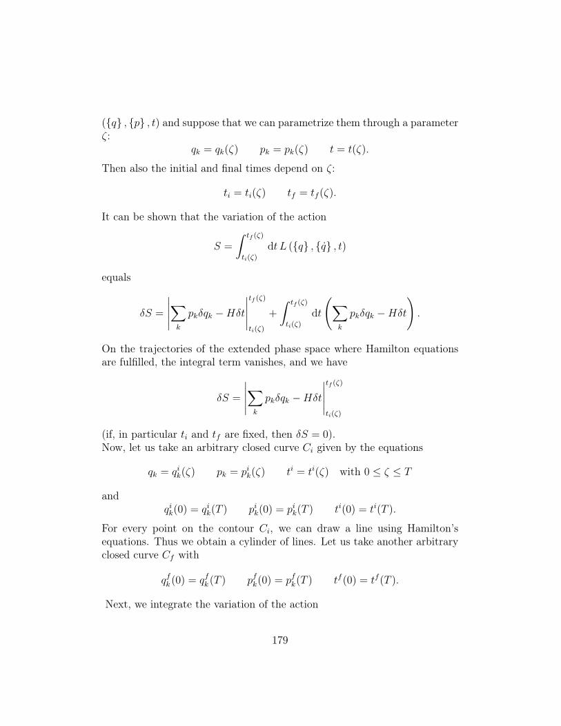
(q , p , t) and suppose that we can parametrize them through a parameterζ:
qk = qk(ζ) pk = pk(ζ) t = t(ζ).
Then also the initial and final times depend on ζ:
ti = ti(ζ) tf = tf (ζ).
It can be shown that the variation of the action
S =
∫ tf (ζ)
ti(ζ)
dt L (q , q , t)
equals
δS =
∣∣∣∣∣∑k
pkδqk −Hδt
∣∣∣∣∣tf (ζ)
ti(ζ)
+
∫ tf (ζ)
ti(ζ)
dt
(∑k
pkδqk −Hδt
).
On the trajectories of the extended phase space where Hamilton equationsare fulfilled, the integral term vanishes, and we have
δS =
∣∣∣∣∣∑k
pkδqk −Hδt
∣∣∣∣∣tf (ζ)
ti(ζ)
(if, in particular ti and tf are fixed, then δS = 0).Now, let us take an arbitrary closed curve Ci given by the equations
qk = qik(ζ) pk = pik(ζ) ti = ti(ζ) with 0 ≤ ζ ≤ T
andqik(0) = qik(T ) pik(0) = pik(T ) ti(0) = ti(T ).
For every point on the contour Ci, we can draw a line using Hamilton’sequations. Thus we obtain a cylinder of lines. Let us take another arbitraryclosed curve Cf with
qfk (0) = qfk (T ) pfk(0) = pfk(T ) tf (0) = tf (T ).
Next, we integrate the variation of the action
179
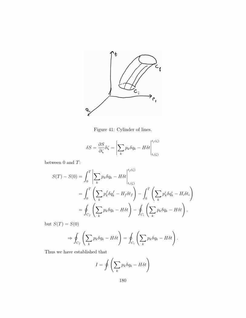
Figure 41: Cylinder of lines.
δS =∂S
∂ζδζ =
∣∣∣∣∣∑k
pkδqk −Hδt
∣∣∣∣∣tf (ζ)
ti(ζ)
between 0 and T :
S(T )− S(0) =
∫ T
0
∣∣∣∣∣∑k
pkδqk −Hδt
∣∣∣∣∣tf (ζ)
ti(ζ)
=
∫ T
0
(∑k
pfkδqfk −Hfδtf
)−∫ T
0
(∑k
pikδqik −Hiδti
)
=
∮Cf
(∑k
pkδqk −Hδt
)−∮Ci
(∑k
pkδqk −Hδt
),
but S(T ) = S(0)
⇒∮Cf
(∑k
pkδqk −Hδt
)=
∮Ci
(∑k
pkδqk −Hδt
).
Thus we have established that
I =
∮ (∑k
pkδqk −Hδt
)
180
is an integral invariant. It is Poincare-Cartan integral invariant (which insome, more geometric, formulations, is considered as the fundamental ob-ject of mechanics). It is possible to show that the canonical transformationscan be obtained from the invariance of the Poincare-Cartan integral. Sev-eral theorems of flows in hydrodynamics also follow from Poincare-Cartanintegral.
If, in particular, we consider contours C of simultaneous states, i.e. wetake the hyperplane of constant time in the cylinder above, then δt = 0 andwe obtain
I1 =
∮ ∑k
pkδqk
which is called Poincare integral invariant.I1 is invariant with respect to any Hamiltonian system. In fact, if for any
system given by the equations
qk = Qk (q , p , t) pk = Pk (q , p , t)
I1 is invariant, it follows that the system is Hamiltonian. Indeed, usingd
dtδq = δq:
d
dtI1 = 0 =
∮ ∑k
(pkδqk + pk
d
dtδqk
)=
∮ ∑k
(pkδqk + pkδqk)
=
∮ ∑k
(pkδqk − qnδpk) ,
thus ∮ ∑k
(Pkδqk −Qkδpk) = 0.
The integrand may be the total differential of some function. If we take thatfunction to be
−H (q , p , t) ,then ∑
k
(pkδqk −Qkδpk) = −δH = −∑k
(∂H
∂qkδqk +
∂H
∂pkδpk
).
181
It follows thatQk =
∂H
∂pkPk = −∂H
∂qkwhich implies that the system is Hamiltonian.
Now, think of Stokes’ theorem in 3 dimensions:∮∂S
A · dl =
∫∫S
(∇× A
)· dS
where ∂S is a contour C which is the boundary of a surface S. In particular,in 2 dimensions,∮
∂S
Ax dx+ Ay dy =
∫∫S
(∂Ay∂x− ∂Ax
∂y
)dx dy
which is also called Green’s theorem.Stokes’ and Green’s theorems (as well as Gauss’ theorem) are all par-
ticular cases of the generalized Stokes’ theorem for differential forms, whichstates that ∫
C=∂S
ω =
∫∫S
dω
i.e. the integral of a form ω on a closed contour C equals the integral of theform dω over the surface S bounded by the contour C.In a nutshell, consider the differential form in 2 dimensions:
ω = A · dl = Ax dx+ Ay dy,
then the derivativedω = dA ∧ dl
is defined through the wedge product ∧, which is linear and antisymmetric,just like the cross product:
a ∧ b = −b ∧ a.
Then
dA ∧ dl = dAx ∧ dx+ dAy ∧ dy
=
:0∂Ax∂x
dx ∧ dx +∂Ax∂y
dy ∧ dx+∂Ay∂x
dx ∧ dy +
*0
∂Ay∂y
dy ∧ dy
=
(∂Ay∂x− ∂Ax
∂y
)dx ∧ dy
182
so ∫A · dl =
∫∫ (∂Ay∂x− ∂Ax
∂y
)dx ∧ dy
where dx∧ dy is the (oriented) area element. For our purposes, we can justtake it to be dx dy. Thus, we got Green’s theorem.
Now, take the form
ω = p · dq = p1 dq1 + · · ·+ pn dqn
in the 2n-dimensional phase space, then
dω = dp ∧ dq = dp1 ∧ dq1 + · · ·+ dpn ∧ dqn.
Then Stokes’ theorem implies∫∂S=C
ω =
∫∫S
dω
⇒ I1 =
∮∂S=C
∑i
pi dqi =
∫∫S
∑i
dpi ∧ dqi ≡ J2
where dpi ∧ dqi are area elements.We have related Poincare integral invariant I1 to a 2-dimensional integral
invariant J2. In fact, this structure can be iterated, i.e. there is an invariantintegral
I3 =
∫∫∫ ∑i,k
piδqiδpkδqk
which can be related to a
J4 =
∫∫∫∫ ∑i,k
δpiδqiδpkδqk
and so on, until one gets to I2n−1 and
J2n =
∫. . .
∫dq1 . . . dqn dp1 . . . dpn
which is of particular interest, because it is the volume element of the phasespace.It is particularly simple to see that J2n is an invariant. In fact, if
dω = dq1 . . . dqn dp1 . . . dpn
183
through a canonical transformation the volume becomes
dΩ = dQ1 . . . dQn dP1 . . . dPn
but dω and dΩ are related by the Jacobian of M:
δΩ = | detM| dω with Mij =dΩi
dωj
and we know thatMTJM = J⇒ (detM)2 = 1
so| detM| = 1⇒ dΩ = dω.
The fact that a volume element is invariant under a canonical transfor-mation immediately implies Liouville’s theorem in statistical mechanics, i.e.that the density of systems around some given system in phase space remainsconstant in time.In fact, the number of systems in a closed neighbourhood of a given systemdoes not change with time; the closed shape just moves about in phase space.Canonical variables at different times are related by a canonical transforma-tion, but we know that the volume element J2n is a canonical invariant, sothe volume size cannot change with time. Therefore the density of systemsis a constant of motion.
Example 13.4. See fig. (42).
184
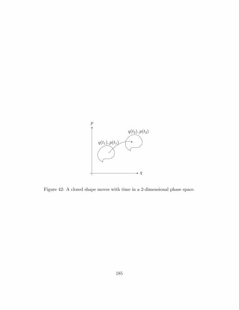
q
p
q(t1), p(t1)
q(t2), p(t2)
Figure 42: A closed shape moves with time in a 2-dimensional phase space.
185
14 Hamilton-Jacobi formalism
14.1 Hamilton-Jacobi equation
Canonical transformations help us to understand the dynamics of a mechan-ical system, i.e. to solve its equations of motion.They can do that in 2 ways:
(a) By transforming the HamiltonianH (q1, . . . , qn; p1, . . . , pn; t) to a Hamil-tonian K (Q1, . . . , Qn;P1, . . . , Pn; t) where all the coordinates Qi arecyclic.In the new variables, Hamilton’s equations are
Qi =∂K
∂PiPi = − ∂K
∂Qi
.
Then, because∂K
∂Qi
= 0, Pi = const. = ci, so the Hamiltonian becomes
K = K (c1, . . . , cn; t) .
Suppose that the Hamiltonian is conserved,
dK
dt=∂K
∂t= 0,
thenQi =
∂K
∂ci= fi (c1, . . . , cn)
which can be trivially integrated to
Qi = fi (c) t+ γi
so the system is fully specified in terms of 2n constants of motion, ciand γi.
(b) The second way is to transform to a set of 2n independent constantsof motion (IEM)
fk (q , p , t) = ck k = 1, . . . , 2n
186
such that
qi = qi (c1, . . . , c2n, t)
pi = pi (c1, . . . , c2n, t)
so the system is completely integrable.The 2n independent IEM might also be the initial conditions such that
qi = qi (q0 , p0 , t)pi = pi (q0 , p0 , t) .
Then one looks for a canonical transformation that maps the set ofvariables (q , p) to the set (q0 , p0).
We shall follow the second avenue: Let us consider a canonical transformationgenerated by the function F (q , P , t) (although the discussion is fullygeneral, and can be done with other generating functions).The transformation equations are:
pi =∂F
∂qiQi =
∂F
∂PiK = H +
∂F
∂t.
Suppose that we have found a function F , such that the new Hamiltonianvanishes:
K = 0 = H +∂F (q , P , t)
∂t.
Then the new equations of motions can be trivially solved:
Qi =∂K
∂Pi= 0 ⇒ Qi = const. = βi
Pi = − ∂K∂Qi
= 0 ⇒ Pi = const. = αi.
The equation for K = 0 is called Hamilton-Jacobi-equation:
H
(q
∂F
∂q
, t
)+∂F
∂t= 0.
It is a 1st-order partial differential equation in (n+ 1) variables: q1, . . . , qn, t.Its solution,
F ≡ S (q1, . . . , qn; t;α1, . . . , αn+1)
187
must be given in terms of n + 1 independent IEM. S is called Hamilton’sprincipal function.Because S appears in the HJ-equation only through the derivatives of Q, ifS is a solution also S +α is a solution. So S is determined up to an additiveconstant, which is irrelevant since the transformation equations are giventhrough derivatives of S,then
S = S (q1, . . . , qn;α1, . . . , αn; t) .
Because the generating function is F (q , P ; t) we may take the newmomenta Pi to be the constants αi
Pi = αi or any combination of them Pi = fi (α1, . . . , αn) .
Then the transformation equations are
pi =∂S (q , α , t)
∂qi(14.1)
Qi = βi =∂S (q , α , t)
∂αi(14.2)
At t = t0, eqs. (14.1) are n equations connecting αi to q0, p0. The βi fromeqs. (14.2) can also be obtained from the initial conditions, by computingthe r.h.s. at t = t0, so one gets
qi = qi (α , β , t)
and through eq. (14.1) also
pi = pi (α , β , t) ,
which solves the system.To understand the physical meaning of S, let us take the time derivative:
dS
dt=∑i
∂S
∂qiqi +
∂S
∂t
=∑i
piqi −H = L.
So, up to a constant, S is the action:
S =
∫L dt+ const..
188
Finally, if the Hamiltonian is conserved,
dH
dt=∂H
∂t= 0,
then the HJ-equation is
H
(q ,
∂S
∂q
)+∂S
∂t= 0
and one can separate the variable t from the others,
S (q , α , t) = W (q , α)− αnt
where W is called Hamilton’s characteristic function.Substituting it into HJ-equation, we get the reduced HJ-equation
H
(q ,
∂W
∂q
)= αn.
For conservative systems, α = E the energy.The physical meaning ofW is understood again by taking the time derivative:
dW
dt=∑i
∂W
∂qiqi =
∑i
piqi.
Integrating gives us
W =∑i
∫dt piqi =
∑i
∫dqipi.
Note that also W generates a canonical transformation, different from theone generated by S. The transformation is
pi =∂W
∂qiQi =
∂W
∂Pi=∂W
∂αiK = H = αn.
ThusW generates a canonical transformation where all coordinates are cyclic.Hamilton’s equations are
Pi = − ∂K∂Qi
= 0 ⇒ Pi = const. = αi
Qi =∂K
∂αi= 0 i = 1, . . . , n− 1 ⇒ Qi = const. = βi
Qn =∂K
∂αn= 1 ⇒ Qn = t+ βn.
189
Note that W (q , α) depends on n constants, but one of them is additivesince in the reduced HJ-equation
H = H
(q ,
∂W
∂q
)= αn.
W appears only through derivatives.So W depends on n − 1 independent constants, say α1, . . . , αn−1 which to-gether with α, form a set of n constants, the new momenta, Pi.To see the difference between the canonical transformations generated by Sand W , draw the prospect:
The Hamiltonian is
H = (q , p , t) an IEM: H = H (q , p)
Look for canonical transformations to (Q , P) such that
Q , P are constants P are constants
Require that the new Hamiltonian
vanishes: K = 0 has K = H = αn, so Qi are cyclic
Hamilton’s equations in the new variables are
Qi =∂K
∂Pi= 0
Pi = − ∂K∂Qi
= 0
Qi =∂K
∂Pi= vi (αi)
Pi = − ∂K∂Qi
= 0
with solutionsQi = βi
Pi = αi
Qi = βi + vi (αi) t
Pi = αi
The generating function is Hamilton’s
principal function S (q , P , t) characteristic func. W (q , P)
HJ-equation is
H
(q ,
∂S
∂q
, t
)H
(q ,
∂W
∂q
)= αn
A complete solution has
190
n non additive constants α1, . . . , αn n − 1 non-additive constantsα1, . . . , αn−1 which together withαn make n independent constants
14.2 Simple harmonic oscillator
The Hamiltonian for the simple harmonic oscillator is
H =1
2m
(p2 +m2ω2q2
)= E with ω =
√k
m.
The Hamilton-Jacobi equation is
1
2m
[(∂S
∂q
)2
+m2ω2q2
]+∂S
∂t= 0.
SincedH
dt= 0, we have the r.h.s. case of the table above, so
S = W − αt with α = E.
The reduced HJ-equation is
1
2m
[(∂W
∂q
)2
+m2ω2q2
]= α
which can be integrated easily to
W =√
2mα
∫dq
√1− mω2q2
2α⇒ S =
√2mα
∫dq
√1− mω2q2
2α−αt.
Also the transformation equation
β =∂S
∂α=
√m
2α
∫dq√
1− mω2q2
2α
− t
can be integrated easily to
β + t =1
ωarcsin q
√mω2
2α
191
that is
q =
√2α
mω2sin(ωt+ γ) with γ = βω
which is the usual solution for the harmonic oscillator.The other transformation equation yields
p =∂S
∂q=√
2mα cos(ωt+ γ).
α and β are related to the initial conditions at t = t0:
α =1
2m
(p2
0 +m2ω2q20
) q0
p0
=1
mωtan(βω)
so Hamilton’s principal function generates a canonical transformation to anew momentum, i.e. the energy, and a new coordinate, i.e. the phase con-stant of the oscillation.
14.3 2-dimensional harmonic oscillator
In two dimensions, the Hamiltonian for the harmonic oscillator is
H =1
2m
(p2x + p2
y +m2ω2xx
2 +m2ω2yy
2)
with ωx =
√kxm
ωy =
√kym
and we have again
dH
dt= 0 ⇒ S (x, y, αx, αy; t) = W (x, y, αx, αy)− αt with α = E.
The reduced HJ-equation is
1
2m
[(∂W
∂x
)2
+
(∂W
∂y
)2
+m2ω2xx
2 +m2ω2yy
2
]= α
which can be separated into
1
2m
[(∂W
∂x
)2
+m2ω2xx
2
]= αx
1
2m
[(∂W
∂y
)2
+m2ω2yy
2
]= αy with α = αx + αy
that can be easily solved.
192
14.4 Separation of variables
In sect. 14.1, we assumed (very wishfully!) that we know Hamilton’s princi-pal function S. But in general it may be very difficult to solve HJ-equation:partial differential equations of many variables are hard to deal with.But with the harmonic oscillator, we saw that a solution can be found ifwe can separate the variables. In fact, that is the case when HJ-equationbecomes a useful tool.Suppose that in the HJ-equation, the coordinate q1 enters only through the
function H1
(q1,
∂S
∂q1
), such that
H
(H1
(q1,
∂S
∂q1
); q2, . . . , qn;
∂S
∂q2
, . . . ,∂S
∂qn; t
)+∂S
∂t= 0,
then q1 is called separable, and we look for a solution of the type
S = S1 (q1;α1, . . . , αn) + S (q2, . . . , qn;α1, . . . , αn; t) .
If we replace it into the HJ-equation, we get the identity
H
(H1
(q1,
∂S1
∂q1
); q2, . . . , qn;
∂S
∂q2
, . . . ,∂S
∂qn; t
)+∂S
∂t= 0.
For this to be true for any q1, it’s necessary and enough to take
H1 = const. = α1.
So we get 2 equations:
H1
(q1,
∂S1
∂q1
)= α1
H
(q2, . . . , qn;
∂S
∂q2
, . . . ,∂S
∂qn;α1; t
)+∂S
∂t= 0.
The first equation is a first-order ordinary differential equation, which is easyto solve. The second equation is still a partial differential equation, but withone less variable. This procedure can be iterated if we have k separablecoordinates q1, . . . , qn.Then the principal function can be written as
S (q1, . . . , qn;α1, . . . , αn; t) =k∑i=1
Si (qi;α1, . . . , αn)+S (qk+1, . . . , qn;α1, . . . , αn; t)
193
and HJ-equation splits into k first order differential equations
Hi
(qi,∂Si∂qi
)= αi i = 1, . . . , k
and the partial differential equation
H
(qk+1, . . . , qn;
∂S
∂qk+1
, . . .∂S
∂qn;α1, . . . , αk; t
)+∂S
∂t= 0.
If all the variables qi and the time t are separable, the principal function canbe written as
S (q1, . . . , qn;α1, . . . , αn; t) =n∑i=1
Wi (qi;α1, . . . , αn)− αt.
The reduced HJ-equation is completely separable and can be written as
H
(H1
(q1,
∂W1
∂q1
); . . . ;Hn
(qn,
∂Wn
∂qn
))= α.
We get n first-order differential equations
Hi
(qi,∂Wi
∂qi
)= αi i = 1, . . . , n
and the conditionH (α1, . . . , αn) = α
where αi are called separation constants.
Note that if q1 is separable and cyclic:∂H
∂q1
= 0, then
H1
(q1,
∂S1
∂q1
)=∂S1
∂q1
= α1 ⇒ S1 = α1q1.
So if k variables are cyclic, the principal function becomes
S =k∑i=1
αiqi + S (qk+1, . . . , qn;α1, . . . , αn; t) .
194
14.5 Action-angle variables
Consider a conservative system with a periodic motion. For simplicity, let ustake it as a function of 2 variables (q, p). The Hamiltonian is
H (q, p) = const. = α.
As new (constant) momentum, let us take Poincare invariant integral
J =
∮p dq.
J is called action variable.Hamilton’s characteristic function is W = W (q, J). The coordinate conju-gate to J is the angle variable w.The transformation equation is
w =∂W
∂Jand w is cyclic.
Hamilton’s equation of motion is
w =∂H(J)
∂J= ν(J)
with ν a constant, and a function of J .As expected, w integrates to
w = νt+ β.
Consider the change in w through a period
∆w =
∮∂W
∂qdq =
∮∂2W
∂q∂Jdq.
Because J is a constant, we can take it out of the integral:
∆w =d
dJ
∮∂W
∂qdq =
d
dJ
∮p dq︸︷︷︸=J
= 1.
So, as q goes through a cycle, w changes by 1. Then
∆w = ντ = 1
195
where τ is the period. So
ν =1
τ
is the frequency of the periodic motion which we have found without solvingthe equations of motion of the system.The discussion can be directly extended to a periodic motion in a 2n-dimensionalphase space, in terms of n action variables
Ji =
∮pi dqi.
196
15 Special RelativitySpecial relativity is based on the assumption that the laws of nature are thesame for inertial observers where their co-ordinates are related via Lorentztransformations:
xµ → xµ′ = Λµνx
ν + ρµ. (15.1)
where
xµ =
x0
x1
x2
x3
(15.2)
a “four-vector” comprising space-time coordinates with x0 = ct, ρµ is a con-stant four-vector and Λµ
ν satisfies:
ΛµρΛ
νσgµν = gρσ. (15.3)
The 4× 4 matrix gµν is the so-called metric, defined as:
gµν =
+1, µ = ν = 0,−1, µ = ν = 1, 2, 30, µ 6= ν
(15.4)
In the above we have used Einstein’s summation convention. For example,one would write explicitly
Λµνx
ν = Λµ0x
0 + Λµ1x
1 + Λµ2x
2 + Λµ3x
3. (15.5)
This is a convention that we will use extensively from now on.
15.1 Proper time
Lorentz transformations leave invariant “proper-time” intervals. These aredefined as:
dτ 2 ≡ c2 dt2 − dx2 = gµν dxµ dxν . (15.6)
Indeed, in a different reference frame we have from Eq. 15.1:
dxµ′ = Λµν dxν . (15.7)
197
A proper-time interval in the new frame is
dτ ′2 = gµν dx′µ dx′ν
= gµν(Λµρ dxρ
)(Λν
σ dxσ)
=(gµνΛ
µρΛ
νσ
)dxρ dxσ
= gρσ dxρ dxσ = dτ 2. (15.8)
As a consequence of the invariance of proper-time intervals, the speed of lightis the same in all inertial frames. Indeed, for light we have:∣∣∣∣dxdt
∣∣∣∣ = c; dτ 2 = c2 dt2 − dx2 = 0 (15.9)
In a new frame,
dτ 2′ = dτ 2 = 0 ;
∣∣∣∣dx′dt′
∣∣∣∣ = c (15.10)
Lorentz transformations are the only non-singular transformations whichpreserve proper-time intervals:
dτ 2 = dτ′2
; gρσ dxρ dxσ = gµν dx′µ dx′ν
; gρσ dxρ dxσ = gµν∂xµ
∂xρ
∂xν
∂xσdxρ dxσ, (15.11)
concluding that:
gρσ = gµν∂xµ
∂xρ
∂xν
∂xσ. (15.12)
Differentiating with dxε, we obtain:
0 = gµν
[∂2x′µ
∂xε∂xρ∂x′ν
∂xσ+
∂2x′µ
∂xε∂xσ∂x′ν
∂xρ
]. (15.13)
To this, we add the same equation with ε↔ ρ and subtract the same equationwith ε↔ σ. We obtain:
0 = 2gµν∂2x′µ
∂xε∂xρ∂x′ν
∂xσ(15.14)
Assuming that the transformation xµ → x′µ is a well behaved differentiablefunction and that the inverse of the transformation also exists,
∂x′µ
∂xσ∂xσ
∂x′ν= δµν , (15.15)
198
we obtain that∂2x′µ
∂xε∂xρ= 0. (15.16)
Therefore, the transformation xµ → x′µ ought to be linear:
x′µ = Λµ ν + ρµ. (15.17)
15.2 Subgroups of Lorentz transformations
The set of all Lorentz transformations
x′µ = Λµνx
ν + ρµ. gµνΛµρΛ
νσ = gρσ (15.18)
form a group (exercise: prove it), which is known as the group of inhomo-geneous Lorentz group or the Poincare’ group. The subset of transformationswith ρµ = 0 is known as the homogeneous Lorentz group.
FromgµνΛ
µρΛ
νσ = gρσ
and for ρ = σ = 0, we have:
(Λ00)2 −
3∑i=1
(Λi0)2 = 1 ; (Λ0
0)2 ≥ 1. (15.19)
Also, in matrix form the definition of the Lorentz transformation becomes:
g = ΛTgΛ ; det g = det(ΛTgΛ) ; (det Λ)2 = 1. (15.20)
The subgroup of transformations with
det Λ = 1, Λ00 ≥ 1,
which contains the unity 1 = δµν , is known as the proper group of Lorentztransformations. All other transformations are known as improper Lorentztransformations. It is impossible with a continuous change of parameters tochange
det Λ = 1→ det Λ = −1 or Λ00 ≥ 1→ Λ0
0 ≤ −1.
Improper Lorentz transformations involve either space-reflection (det Λ =−1,Λ0
0 ≥ 1) or time-inversion (det Λ = 1,Λ00 ≤ −1) or both (det Λ =
−1,Λ00 ≤ −1).
199
Proper homogeneous or inhomogeneous Lorentz transformations have afurther subgroup: the group of rotations,
Λ00 = 1, Λi
0 = Λ0i = 0, Λi
j = Rij, (15.21)
withdetR = 1, RTR = 1. (15.22)
Thus, for rotations and translations (xµ → x′µ = xµ + ρµ) Lorentz transfor-mations are no different than Galilei transformations.
A difference with Galilei transformations arises in boosts. Assume a ref-erence frame O in which a certain particle appears at rest, and O′ a referenceframe where the particle appears to move with a velocity v. Space-timeintervals in the two frames are related via
dx′µ = Λµν dxν = Λµ
0c dt, (15.23)
given that dx = 0 in the frame O. For µ = 0, this equation gives
dt′ = Λ00 dt. (15.24)
For µ = i = 1, 2, 3 we have:
dx′i = Λi0c dt (15.25)
Dividing the two, we have
vi ≡ dx′i
dt′= c
Λi0
Λ00
; Λi0 =
vi
cΛ0
0. (15.26)
FromgµνΛ
µρΛ
νσ = gρσ
and for ρ = σ = 0, we have:
(Λ00)2 − (Λi
0)2 = 1
; Λ00 = γ =
(1− v2
c2
)− 12
. (15.27)
and thusΛi
0 = γvi
c. (15.28)
200
The remaining components are not determined uniquely by knowing the ve-locity v of the particle. Indeed, two Lorentz transformations
Λµν and Λµ
ρRρν
where R is a rotation, boost a particle to the same velocity. For coordinatesystems O and O′ with parallel axes we find that (exercise)
Λij = δij +
vivj
v2(γ − 1) (15.29)
andΛ0j = γ
vj
c. (15.30)
15.3 Time dilation
Consider an inertial observer O which looks as a clock at rest. Two ticks ofthe clock correspond to a space-time interval
dx = 0, dt = ∆t. (15.31)
The proper time interval is
dτ = (c2 dt2 − dx2)12 = c∆t. (15.32)
A second observer sees the clock with velocity v. Two ticks of the clockdefine a space-time interval
dt′ = ∆t′, dx′ = v dt′. (15.33)
The proper-time interval in the new frame is:
dτ ′ = (c2 dt′2 − dx′2)12 = c∆t′
√1−
∣∣∣∣ dx′
cdt′
∣∣∣∣2 = c∆t′√
1− v2
c2. (15.34)
The proper-time is invariant under the change of inertial reference frames.Thus we conclude that
∆t′ =∆t√1− v2
c2
= γ∆t (15.35)
201
15.4 Doppler effect
Take our clock to be a source of light with a frequency
ω =2π
∆t.
For an observer where the light-source is moving with velocity v this timeinterval is measured to be
dt′ = γ∆t.
In the same period, the distance of the observer from the light source increasesby
vr dt′
where vr is the component of the velocity of the light-source along the direc-tion of sight of the observer. The time elapsing between the reception of twosuccessive light wave-fronts from the observer is
c dt0 = c dt′ + vr dt′. (15.36)
The frequency measured by the observer is
ω′ =2π
dt0=
√1− v2
c2
1 + vrc
ω. (15.37)
If the light-source is moving along the line of sight, vr = v, we have
ω′ =
√1− v
c
1 + vc
ω. (15.38)
If the light-source moves away from the observer, vr > 0, the frequencydecreases and the light appears to be more red (red shift). If the sourcemoves towards the observer, the frequency increases (violet shift).
Exercise 15.1. Calculate the angle of the direction of motion of the light-source with respect to the line of sight of the observer for which there is noshift in the frequency.
For an application of the Doppler effect in cosmology, read about Hubble’s law.
202
15.5 Particle dynamics
How can we compute the force of a particle which moves with a relativisticvelocity v? We should expect that our classical formulae from Newtonianmechanics need to be modified. On the other hand, Newtonian expressionsfor the force should be valid if a particle is at rest. We can always changereference frame with Lorentz transformations to bring a particle at rest andcalculate the change in its velocity for a small time interval using Newtonianmechanics. However, we will need to perform these changes of reference frameat every small increase of the velocity of the particle during its accelerationdue to the force.
In a more elegant solution to the problem, we define a relativistic forceacting on a particle as
fµ = mc2 d2xµ
dτ 2, (15.39)
where m is the mass of a particle 3. If the particle is at rest, the proper-timeinterval dτ coincides with the common time-interval dt
dτ = c dt.
Therefore, in the rest frame of the particle, the“space”-components of theforce four-vector become
f irest = md2xi
dt2= F i
Newton, for i = 1, 23, (15.40)
where FNewton is the force-vector as we know it from Newtonian mechanics.The “time” component of the force four-vector vanishes:
f 0rest = mc
d2t
dt2= 0. (15.41)
Under a Lorentz transformation, fµ transforms as
fµ = mc2 d2xµ
dτ 2→ mc2 d2x′µ
dτ 2= mc2 d2 (Λµ
νxν + ρµ)
dτ 2= Λµ
νmc2 d2xν
dτ 2(15.42)
Therefore,f ′µ = Λµ
νfν . (15.43)
3With mass, we mean the mass of a particle as it is measured in its rest-frame. We willrefrain from using the “relativistic”, velocity dependent, mass.
203
The components of fµ transform under Lorentz transformations in exactlythe same way as the components of space-time coordinates. It is therefore afour-vector as well.
For a specific transformation from the rest frame of a particle to a framewhere the particle moves with a velocity v, we have
fµ = Λµν(v)f νrest. (15.44)
where, we have found that,
Λ00(v) = γ =
(1− v2
c2
)− 12
, Λi0(v) = Λ0
i(v) = γvi
c.
Λij(v) = δij +
vivj
v2(γ − 1) (15.45)
Therefore, the force on a moving particle is:
f = FNewton + (γ − 1)v(FNewton · v
)v2
, (15.46)
and
f 0 = γv · FNewton
c=v
c· f. (15.47)
In Newtonian mechanics, if the force F is given, we can compute thetrajectory x(t) by solving the second order differential equation:
d2x
dt2=F (x, t)
m. (15.48)
Similarly, in special relativity, when the relativistic force fµ is known, thedifferential equation 15.39 can, in principle, be solved to give the space-timecoordinates as a function of the proper time τ :
xµ = xµ(τ). (15.49)
To calculate the trajectory, we then need to calculate the proper-time interms of the time coordinate by inverting
x0 = x0(τ) ; τ = τ(x0), (15.50)
204
which we can use to cast the space components directly as functions of thetime-coordinate.
We should not forget a second constrain that must be satisfied for oursolutions xµ(τ), namely
Ω ≡ gµνdxµ
dτ
dxν
dτ= 1. (15.51)
We have for the derivative of Ω with respect to proper-time:
dΩ
dτ= 2gµν
d2xµ
dτ 2
dxν
dτ=
2
mc2gµνf
µdxν
dτ. (15.52)
The rhs is a Lorentz invariant quantity. In a new frame,
gµνf′µdx′ν
dτ= gµν
(Λµρf
ρ) (Λν
σdxσ)
dτ=(gµνΛ
µρΛ
νσ
)fρ
dxσ
dτ= gρσf
ρdxσ
dτ.
We are therefore allowed to computedΩ
dτin any reference frame we wish. Let
us choose the rest frame of the particle, where
xµ = (ct, 0), fµ = (0, FNewton).
We obtain:dΩ
dτ=
2
mc2
(f 0 dx0
dτ− f · x
)= 0. (15.53)
Therefore, the quantity Ω is always a constant:
Ω(τ) = constant. (15.54)
If for some initial value τ0 we choose the constant to be one, we will have
Ω(τ) = Ω(τ0) = 1, ∀ τ. (15.55)
Exercise 15.2. Calculate the trajectory of a particle on which the four-vector force exerted is fµ = 0.
205
15.6 Energy and momentum
We can define a relativistic four-vector analogue of momentum as
pµ = mcdxµ
dτ(15.56)
We have that
dτ =(c2 dt2 − dx2
) 12 = c dt
[1−
(dx
c dt
)2] 1
2
= c dt
[1− v2
c2
] 12
=c dt
γ.
(15.57)Thus, for the time-component (µ = 0) of the four-momentum we have
p0 = mcdx0
dτ= mγc. (15.58)
For the space-components (µ = i = 1, 2, 3) we have
pi = mcdxi
dτ= mγ
dxi
dt= mγvi. (15.59)
For small velocities, we can expand the factor γ as
γ =
[1− v2
c2
]− 12
≈ 1 +1
2
v2
c2+O
(v4
c4
). (15.60)
Therefore, for small velocities the space-components of the four-momentumbecome the classical momentum,
pi ≈ mvi + . . . , (15.61)
while the time-component becomes
p0 ≈ mc+1
2cmv2 + . . . (15.62)
In the second term of the above expansion we recognize the kinetic energy12mv2 of the particle. We then identify the relativistic energy of a particle
withE = cp0 = mγc2. (15.63)
Eliminating the velocity v from Eqs 15.59-15.63, we obtain the relation:
E =√p2c2 +m2c4 (15.64)
206
15.7 The inverse of a Lorentz transformation
Recall the metric matrix
gµν = diag(1,−1,−1,−1) (15.65)
We define an inversegµν : gµνgνρ = δµν , (15.66)
where δµν is the Kronecker delta. It is easy to verify that the inverse of themetric is the metric itself:
gµν = gµν = diag(1,−1,−1,−1). (15.67)
Now consider a Lorentz transformation Λµν , which satisfies the identity:
ΛµρΛ
νσgµν = gρσ. (15.68)
We can prove that the matrix
Λ νµ ≡ gµρg
νσΛρσ (15.69)
is the inverse of Λµν . Indeed
ΛµλΛ
νµ = gµρg
νσΛρσΛµ
λ = gσλgνσ = δλν . (15.70)
If Λµν is a velocity v boost transformation of Eq. 15.45, then
Λ 00 (v) = γ =
(1− v2
c2
)− 12
, Λ 0i (v) = Λ i
0 (v) = −γ vi
c.
Λ ji (v) = δji +
vivj
v2(γ − 1) (15.71)
We, therefore have that the inverse of a boost is
Λ νµ (v) = Λµ
ν(−v), (15.72)
as we also expect physically.
207
15.8 Vectors and Tensors
It is now time to give officially a definition for vectors in special relativity.We call any set of four components which transform according to the rule:
V µ → V ′µ = ΛµνV
ν (15.73)
a contravariant vector. Contravariant vectors transform in the same way asspace-time coordinates xµ do under homogeneous Lorentz transformations.
Not all vectors transform as contravariant vectors. Consider the derivative∂∂xµ
. Under a Lorentz transformation, it transforms as:
∂
∂xµ→ ∂
∂x′µ=∂xρ
∂x′µ∂
∂xρ. (15.74)
We have that (∂xρ
∂x′µ
)(∂x′µ
∂xν
)= δρν ;
(∂xρ
∂x′µ
)Λµν = δρν . (15.75)
Therefore,(∂xρ
∂x′µ
)is the inverse of a Lorentz transformation Λµ
ν :
∂xν
∂x′µ= Λ ν
µ . (15.76)
Substituting into Eq. 15.74, we find:
∂
∂xµ→ ∂
∂x′µ= Λ ρ
µ
∂
∂xρ. (15.77)
We found that the derivative does not transform according to the Lorentztransformation but according to its inverse. All vectors which transform withthe inverse Lorentz transformation:
Uµ = Λ νµ Uν , (15.78)
are called covariant vectors.For every contravariant vector Uµ there is a dual vector
Uµ = gµνUν . (15.79)
We can invert the above equation multiplying with gρµ,
gρµUµ = gρµgµνUν = δρνU
ν = Uρ. (15.80)
208
The dual vector Uµ is a covariant vector. Indeed, under a Lorentz transfor-mation we have
Uµ → U ′µ = gµνU′ν = gµνΛ
νρU
ρ = gµνΛνρgρσUσ = Λ σ
µ Uσ. (15.81)
The scalar product of a contravariant and a covariant vector
A ·B ≡ AµBµ = AµBµ = gµνA
µBν = gµνAµBν (15.82)
is invariant under Lorentz transformations. Indeed,
A ·B → A′ ·B′ = A′µB′µ = ΛµρA
ρΛ σµ Bσ = δσρA
ρBσ = AρBρ = A ·B. (15.83)
Let us define for short:∂µ ≡
∂
∂xµ, (15.84)
and the dual contravariant vector:
∂µ =∂
∂xµ= gµν∂ν . (15.85)
The D’ Alembert operator is the scalar product:
2 ≡ ∂2 ≡ ∂µ∂µ =
1
c2
∂2
∂t2−∇2. (15.86)
Due to it being a scalar product, the D’Alembert operator is invariant underLorentz transformations.
Finally, we define a tensor with multiple “up” and/or “down” indices tobe an object
T µ1µ2...ν1ν2...(15.87)
which transfroms as:
T µ1µ2...ν1ν2...→ Λµ1
ρ1Λµ2ρ2. . .Λ σ1
ν1Λ σ2ν2. . . T ρ1ρ2...σ1σ2...
(15.88)
209
![Classical Mechanics - people.phys.ethz.chdelducav/cmscript.pdf · References [1]LandauandLifshitz,Mechanics,CourseofTheoreticalPhysicsVol.1., PergamonPress [2]Classical Mechanics,](https://img.pdfslide.net/doc/110x75/5e1e9832bac1ea74484e9601/classical-mechanics-delducavcmscriptpdf-references-1landauandlifshitzmechanicscourseoftheoreticalphysicsvol1.jpg)


![[Kibble] - Classical Mechanics](https://img.pdfslide.net/doc/110x75/552056344a79596f718b4715/kibble-classical-mechanics.jpg)