Embed Size (px)
Citation preview

LECTURE NOTES - WINTER SEMESTER 2019/20
Classical Methods for Partial DifferentialEquations
PROF. DR. MICHAEL PLUM
PRELIMINARY UNOFFICIAL AND uncorrected VERSION : FEBRUARY 7, 2020
DIGITALIZATION: MARIE M. S. PEREIRA
Contents1 Basic concepts, examples 2
1.1 Examples from mathematical physics . . . . . . . . . . . . . . . . . . . . . . . 2
2 Initial value problem for the wave equation (in spatial dimensions 1, 2, 3) 112.1 Spatially 1D wave equation . . . . . . . . . . . . . . . . . . . . . . . . . . . . . 112.2 The wave equation in R3 . . . . . . . . . . . . . . . . . . . . . . . . . . . . . . 162.3 The wave equation in R2 . . . . . . . . . . . . . . . . . . . . . . . . . . . . . . 232.4 The inhomogeneous wave equation . . . . . . . . . . . . . . . . . . . . . . . . . 252.5 Separation of variables . . . . . . . . . . . . . . . . . . . . . . . . . . . . . . . 27
3 Potential and Poisson equation 38
4 The heat equation 614.1 Maximum Principle for heat equation on spatially bounded domain . . . . . . . . 68
5 Type classification of second order partial differential equations with two indepen-dent variables 715.1 Computation of characteristic curves in the semilinear case . . . . . . . . . . . . 73
6 Normal forms for semilinear PDE’s of second order in R2 86
7 An existence and uniqueness result for the semilinear hyperbolic initial value prob-lem 94
8 Type classification for semi linear second oeder differential equations in n variables102

1 Basic concepts, examplesA differential equation is a relation of the form
F
(x1, . . . , xn, u,
∂u
∂x1
, . . . ,∂u
∂xn,∂2u
∂x21
,∂2u
∂x1∂x2
, . . . ,∂2u
∂x2n
,∂3u
∂x31
,∂3u
∂x21∂x2
, . . . ,∂3u
∂x3n
, . . . ,∂mu
∂xmn
)= 0
with a given function F : D → Rk, D ⊂ RN , N suitable, which really depends on at least oneof the components from ∂u
∂x1onwards. If n ≥ 2 and if F really depends on variables in which
derivatives with respect to different xi are present, for example ∂u∂x1
and ∂u∂x2
, or ∂2u∂x1∂x2
, the dif-ferential equation is called partial differential equation (PDE), otherwise ordinary differentialequation (ODE).
If F really depends on one of the components ∂mu∂xm1
, ∂mu∂xm−1
1 ∂x2, . . . , ∂
mu∂xmn
, then m is called theorder of the differential equation.
For k ≥ 2, the differential equation is also called system of differential equations. We arelooking for a function u : Ω→ Rl with a suitable set Ω ⊂ Rn, the derivatives of which, occurringin the differential equation, exists in some suitable sense, the values
(x1, . . . , xn, u(x1, . . . , xn), ∂u∂x1
(x1, . . . , xn), . . . , ∂mu∂xmn
(x1, . . . , xn)) of which are in D for all(x1, . . . , xn) ∈ Ω, and which satisfies the differential equation for all (x1, . . . , xn) ∈ Ω.
If F depends linearly on all components from u onwards, i.e. if the differential equation hasthe form
a(0)(x1, . . . , xn)u+ a(1)1 (x1, . . . , xn)
∂u
∂x1
+ · · ·+ a(1)n (x1, . . . , xn)
∂u
∂xn+ a
(2)11
∂2u
∂x21
+ . . .
+ a(2)nn
∂2u
∂x2n
+ · · ·+ a(m)(1,...,1)(x1, . . . , xn)
∂mu
∂xn1+ · · ·+ a
(m)(n,...,n)
∂mu
∂xmn− r(x1, . . . , xn) = 0
the differential equation is called linear, otherwise nonlinear. In the linear case, the functionsamn (x1, . . . , xn) are called coefficients of the differential equation.
If F depends linearly on the highest derivatives (i.e. the m-th derivatives), but arbitrarily onlower derivatives, the differential equation is called semilinear. If the differential equation hasthe form of a semilinear one, but with coefficients (of the highest order derivatives) depending notonly on x1, . . . , xn, but also on u and its derivatives up to order m − 1, the differential equationis called quasilinear.
1.1 Examples from mathematical physicsIn this example section, we do not care about smoothness of the occurring functions, but assumethat all used derivatives exist.
Example 1.1. Maxwell’s equation (electro- dynamics), here only in vacuum.Given: charge density ρ : R3 × [0,∞) → R, current density j : R3 × [0,∞) → R3. We are
looking for the electrical field E : R3 × [0,∞)→ R3 and the magnetic field B : R3 × [0,∞)→R3.
2
Maxwell’s equations:
divE = 4πρ, curlE = −∂B∂t, divB = 0, curlB =
∂E
∂t+ 4πj
(curl ≡ rotgerman) (Speed of light is normalized to 1).So we have n = 4, m = 1, k = 8, l = 6, u =
(EB
).
- We have div curl ≡ 0, and there holds some converse statement as well:If div v ≡ 0 on R3 (sufficient: on a simply connected domain) then there exists w such thatv = curlw (here without proof and without specification of smoothness properties).
- We have curl grad ≡ 0, and there holds some converse statement as well:If curl v ≡ 0︸ ︷︷ ︸⇔ ∂vi∂xj
=∂vj∂xi
on R3, then there exists ϕ such that v = gradϕ. (proof: see Analysis II)
Now we proceed with Maxwell’s equations. From divB = 0 we therefore have: There existsa vector potential A : R3 × [0,∞)→ R3 such that
B = curlA (1)
Insert (1) into curlE = −∂B∂t
:
curlE = −∂ curlA
∂t= − curl
(∂A
∂t
), i.e. curl
(E +
∂A
∂t
)= 0.
So there exists a scalar potential φ : R3 × [0,∞)→ R such that
E +∂A
∂t= − gradφ (“−”: physical convention) (2)
Insert (2) into divE = 4πρ :
4πρ = div
(− gradφ− ∂A
∂t
)= −∆φ− div
(∂A
∂t
),
where ∆ is the Laplace operator defined by
∆u :=n∑i=1
∂2u
∂x2i
= div gradu.
So we have
−∆φ = 4πρ+∂
∂tdivA (3)
3

Insert (1) and (2) into curlB = ∂E∂t
+ 4πρ :
curl curlA = − ∂
∂tgradφ︸ ︷︷ ︸
=grad ∂φ∂t
−∂2A
∂t2+ 4πj.
Since curl curlu = grad div u− div gradu︸ ︷︷ ︸=∆u
:
grad divA−∆A = −∂2A
∂t2− grad
(∂φ
∂t
)+ 4πj, i.e.
∂2A
∂t2−∆A = − grad
(∂φ
∂t+ divA
)+ 4πj. (4)
If A and φ solve equations (1) and (2), then also
A = A+ gradϕ, φ = φ− ∂ϕ
∂t
(with arbitrary ϕ) solve equations (1) and (2) (for (2): ∂∂t
gradϕ is added on both sides).Prescribing ϕ means ”gauging” the differential equations (3) and (4).
Coulomb gauge: Try to obtain div A = 0, i.e. divA+div gradϕ︸ ︷︷ ︸∆ϕ
!= 0, which is a differential
equation for ϕ. So the remaining equations (3) and (4) are
−∆φ = 4πρ, Poisson equation, potential equation. For ρ = 0: Laplace equation (5)
and
∂2A
∂t2−∆A = − grad
(∂φ
∂t
)+ 4πj, wave equation for A. (6)
These equations (5), (6) are not Lorentz invariant.
Lorentz gauge: Try to obtain div A + ∂φ∂t
= 0, i.e. div (A+ gradϕ) + ∂φ∂t− ∂2ϕ
∂t2= 0, i.e.
∂2ϕ∂t2−∆ϕ = divA+ ∂φ
∂twave equation for ϕ; can be solved in a suitable sense.
Then equations (3) and (4) become
∂2φ
∂t2−∆φ = 4πρ (7)
∂2A
∂t2−∆A = 4πj (8)
4
These are wave equations for both electric and magnetic potential.From these, also wave equations for E and B can be derived (exercises). The solution of
these are the famous electro-magnetic waves.
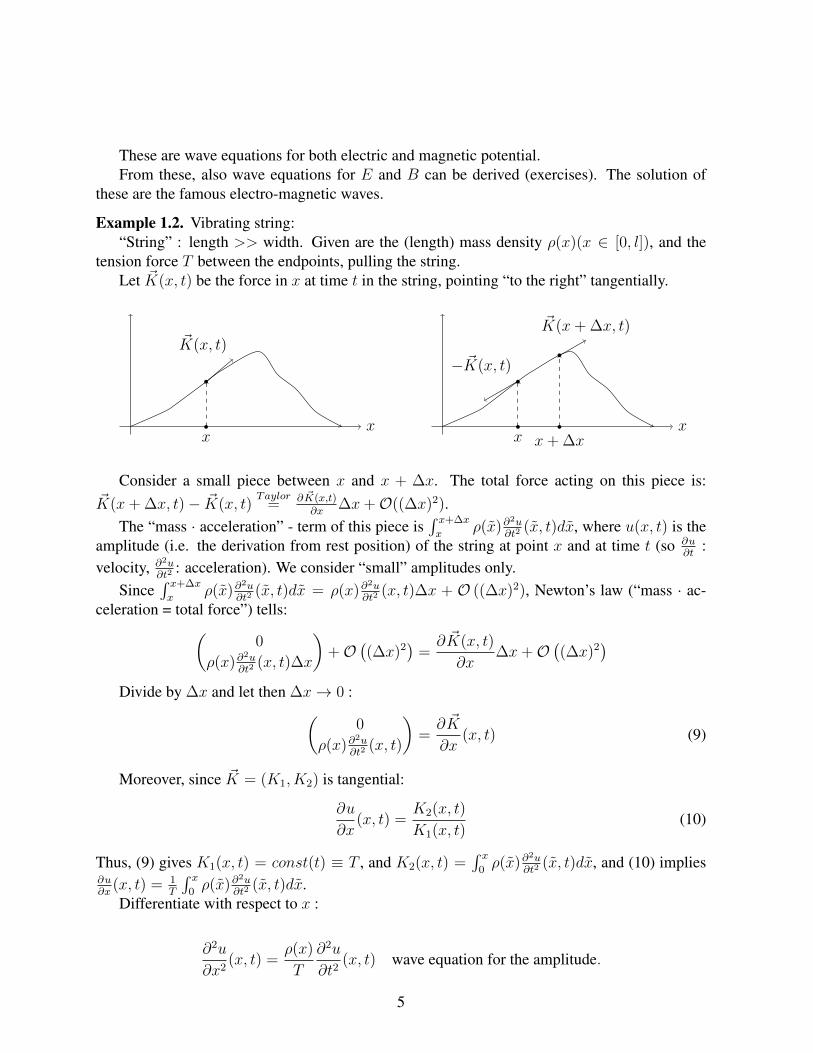
Example 1.2. Vibrating string:“String” : length >> width. Given are the (length) mass density ρ(x)(x ∈ [0, l]), and the
tension force T between the endpoints, pulling the string.Let ~K(x, t) be the force in x at time t in the string, pointing “to the right” tangentially.
~K(x, t)
xx
~K(x+ ∆x, t)
− ~K(x, t)
x x+ ∆xx
Consider a small piece between x and x + ∆x. The total force acting on this piece is:~K(x+ ∆x, t)− ~K(x, t)
Taylor= ∂ ~K(x,t)
∂x∆x+O((∆x)2).
The “mass · acceleration” - term of this piece is∫ x+∆x
xρ(x)∂
2u∂t2
(x, t)dx, where u(x, t) is theamplitude (i.e. the derivation from rest position) of the string at point x and at time t (so ∂u
∂t:
velocity, ∂2u∂t2
: acceleration). We consider “small” amplitudes only.Since
∫ x+∆x
xρ(x)∂
2u∂t2
(x, t)dx = ρ(x)∂2u∂t2
(x, t)∆x + O ((∆x)2), Newton’s law (“mass · ac-celeration = total force”) tells:(
0
ρ(x)∂2u∂t2
(x, t)∆x
)+O
((∆x)2
)=∂ ~K(x, t)
∂x∆x+O
((∆x)2
)Divide by ∆x and let then ∆x→ 0 :(
0
ρ(x)∂2u∂t2
(x, t)
)=∂ ~K
∂x(x, t) (9)
Moreover, since ~K = (K1, K2) is tangential:
∂u
∂x(x, t) =
K2(x, t)
K1(x, t)(10)
Thus, (9) gives K1(x, t) = const(t) ≡ T , and K2(x, t) =∫ x
0ρ(x)∂
2u∂t2
(x, t)dx, and (10) implies∂u∂x
(x, t) = 1T
∫ x0ρ(x)∂
2u∂t2
(x, t)dx.Differentiate with respect to x :
∂2u
∂x2(x, t) =
ρ(x)
T
∂2u
∂t2(x, t) wave equation for the amplitude.
5
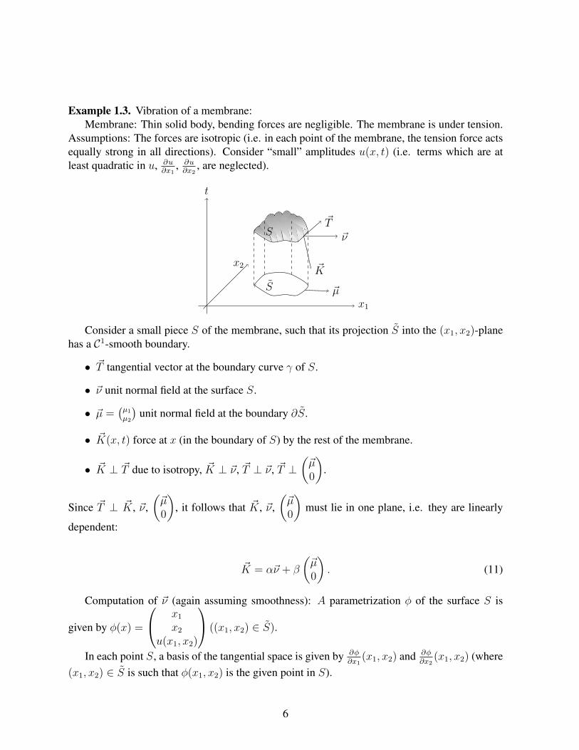
Example 1.3. Vibration of a membrane:Membrane: Thin solid body, bending forces are negligible. The membrane is under tension.
Assumptions: The forces are isotropic (i.e. in each point of the membrane, the tension force actsequally strong in all directions). Consider “small” amplitudes u(x, t) (i.e. terms which are atleast quadratic in u, ∂u
∂x1, ∂u∂x2
, are neglected).
~T~ν
~K
~µS
S
x1
t
x2
Consider a small piece S of the membrane, such that its projection S into the (x1, x2)-planehas a C1-smooth boundary.
• ~T tangential vector at the boundary curve γ of S.
• ~ν unit normal field at the surface S.
• ~µ =(µ1
µ2
)unit normal field at the boundary ∂S.
• ~K(x, t) force at x (in the boundary of S) by the rest of the membrane.
• ~K ⊥ ~T due to isotropy, ~K ⊥ ~ν, ~T ⊥ ~ν, ~T ⊥(~µ0
).
Since ~T ⊥ ~K, ~ν,(~µ0
), it follows that ~K, ~ν,
(~µ0
)must lie in one plane, i.e. they are linearly
dependent:
~K = α~ν + β
(~µ0
). (11)
Computation of ~ν (again assuming smoothness): A parametrization φ of the surface S is
given by φ(x) =
x1
x2
u(x1, x2)
((x1, x2) ∈ S).
In each point S, a basis of the tangential space is given by ∂φ∂x1
(x1, x2) and ∂φ∂x2
(x1, x2) (where(x1, x2) ∈ S is such that φ(x1, x2) is the given point in S).
6
We know: ∂φ∂x1
=
10∂u∂x1
, ∂φ∂x2
=
01∂u∂x2
. By “inspection” or by taking the cross product,
we find that
− ∂u∂x1
− ∂u∂x2
1
is orthogonal to ∂φ∂x1
and ∂φ∂x2
. So since ν3 > 0 and |ν| = 1 :
ν =1√(
∂u∂x1
)2
+(∂u∂x2
)2
+ 1
− ∂u∂x1
− ∂u∂x2
1
.
Since ~K ⊥ ~ν, we have K3 = K1 · ∂u∂x1+K2 · ∂u∂x2
, i.e. by (11) :
~K = α
− ∂u∂x1
− ∂u∂x2
1
+ β
µ1
µ2
0
, so α = K3 = K1 ·∂u
∂x1
+K2 ·∂u
∂x2
, and hence
(K1
K2
)=
− ∂u∂x1
(K1 · ∂u∂x1
+K2 · ∂u∂x2
)− ∂u∂x2
(K1 · ∂u∂x1
+K2 · ∂u∂x2
)︸ ︷︷ ︸
neglected since of order 2 in u.
+β
(µ1
µ2
)≈ β
(µ1
µ2
), so
~K =
β
(µ1
µ2
)K1 · ∂u∂x1
+K2 · ∂u∂x2
= β
µ1
µ2∂u∂x1µ1 + ∂u
∂x2µ2
= β
(~µ
(gradu) · ~µ
).
So the total force acting on the piece S is
∫∂S
~Kdσ =
∫∂S
β
(~µ
(gradu) · ~µ
)dσ =
∫∂Sβµ1dσ∫
∂Sβµ2dσ∫
∂Sβ(gradu) · ~µdσ
Gauss=
∫S∂β∂x1dx∫
S∂β∂x2dx∫
Sdiv(β gradu)dx
.
On the other hand, the “mass · acceleration” term of the piece S is
00∫
Sρ(x)∂
2u∂t2
(x, t)dx
.
So by Newton’s law, we have
∫S∂β∂x1dx∫
S∂β∂x2dx∫
Sdiv(β gradu)dx
=
00∫
Sρ(x)∂
2u∂t2
(x, t)dx
i.e. ,
7
∫S∂β∂x1dx =
∫S∂β∂x2dx = 0 and
∫S
[ρ∂
2u∂t2− div(β gradu)
]dx = 0.
Since S is arbitrary (up to the requirement of a C1-boundary ), we obtain ∂β∂x1≡ ∂β
∂x2≡ 0,
i.e. β is constant, and ρ∂2u∂t2− div(β gradu)︸ ︷︷ ︸
=β div gradu=β∆u
≡ 0, i.e.∂2u
∂t2=β
ρ∆u two-dimensional wave
equation.
Example 1.4. Heat equation:Let K be a solid body in R3. We are looking for the temperature distribution u(x, t) for
x ∈ K, t ≥ 0. Given is a heat source distribution q(x, t) (for example, by an electric current orby a chemical reaction).
Crucial quantity:
Heat flux ~Φ = −α gradu,
α > 0 heat diffusion coefficient (often x-dependent, if K is not homogeneous, sometimes evenu-dependent). Let Ω ⊂ K be a “small piece” (domain) with ∂Ω in C1. The amount of heat insideΩ is
∫Ωβ(x)u(x, t)dx, where β is the specific heat.
The decrease of heat in Ω per unit time is:
(i)− d
dt
∫Ω
β(x)u(x, t)dx, (ii)−∫
Ω
q(x, t)dx+
∫∂Ω
~Φ · ~νdσ,
so we have
−∫
Ω
β(x)∂u
∂tdx = −
∫Ω
q(x, t)dx+
∫∂Ω
~Φ · ~νdσ︸ ︷︷ ︸=−
∫∂Ω(α gradu)·~νdσGauss= −
∫Ω div(α gradu)dx
i.e. ∫Ω
[β∂u
∂t− div(α gradu)− q
]dx = 0.
Since Ω is arbitrary, we conclude as before:
β∂u
∂t− div(α gradu) = q (x ∈ K, t ≥ 0)
If α depends on u, this equation is quasilinear.If α is constant, the equation reads ∂u
∂t− α
β∆u = q
β(inhomogeneous) heat equation.
If the temperature is not time dependent: −∆u = 1αq stationary heat equation; Poisson equa-
tion.
8

Often (or even in most cases) there are boundary conditions which are added to the differ-ential equation.
For example, in our heat flow problem:Heat flux through the boundary of K (from inside to outside) ∼ temperature difference be-
tween inside and outside temperature ua (constant), i.e.
~Φ︸︷︷︸=−α(gradu)
·~ν = γ(u(x, t)− ua), which reads(
note (gradu) · ~ν =:∂u
∂ν
)α∂u
∂ν+ γu = γua, i.e.
∂u
∂ν+ γu = γua, for x ∈ ∂K, t ≥ 0.
γ = γα∼ heat conductivity.
Special cases:
(i) γ → ∞: Boundary condition turns into u = ua on ∂K (t ≥ 0): infinite heat conduc-tivity on ∂K keeps it always on outside temperature. This boundary condition is calledDirichlet boundary condition or boundary condition of the first kind: u is prescribed onthe boundary.
(ii) γ = 0: ∂u∂ν
= 0 on ∂K (t ≥ 0): no heat conductivity on ∂K, no heat flux to outside world.This boundary condition is called Neumann boundary condition or boundary condition ofthe second kind or isolating boundary condition: ∂u
∂νis prescribed on the boundary.
(iii) 0 < γ < ∞: real situation, which however is often idealized by (i) or (ii). This boundarycondition is called Robin boundary condition or boundary condition of the third kind.
(iv) The boundary conditions (i),(ii), (iii) may all occur on different parts of the boundary.This boundary condition is called mixed boundary condition or boundary condition of thefourth kind.
Also the other examples treated in this example section have associated boundary conditions:
(1.1)(Maxwell) If ρ and j have compact support with respect to x, then E, B, A, Φ (andpossibly also some derivatives of these) are required to vanish as |x| → ∞ stronger than 1
|x|2 .But sometimes it makes sense to study electro-dynamics on a bounded domain Ω ⊂ R3 (or betterΩ × [0,∞)). For example, for the electric potential Φ, then the following boundary conditionsmay occur:
(i) Φ = 0 on ∂Ω: ∂Ω is put on earth.
(ii) ∂Φ∂ν
= 0 on ∂Ω: ∂Ω is isolated.
9

Example 1.5. Faraday’s cageIn the interior of the cage C there are no charges (ρ ≡ 0) and no currents (j ≡ 0), and the
situation is stationary. Then we have (by Maxwell’s equation and the definition of the electricpotential [E = − gradφ]): ∆φ = 0.
Moreover, the boundary of the cage is put on earth (φ = 0 on ∂C) or is isolated (∂φ∂ν
= 0 on∂C).
0 =
∫C
(∆φ)︸ ︷︷ ︸=0
φdxGreen′sformula
=
∫∂C
∂φ
∂νφ︸︷︷︸
=0
dσ −∫C
(gradφ) · (gradφ)dx = −∫C
| gradφ|2︸ ︷︷ ︸≥0
dx
So we have gradφ ≡ 0, so sinceC is connected: φ ≡ constant⇒ E ≡ 0⇒ no voltage insideC.
(1.2) (vibrating string) u(0, t) = u(l, t) = 0 Dirichlet boundary conditions.
(1.3) (vibrating membrane) u(x, t) = 0 ∀x ∈ ∂(membrane) Dirichlet boundary conditions.
For the time dependent problems, initial conditions have to be added (usually for t = 0)
- heat equation: u(x, 0) = u0(x) (x ∈ K), u0 is a precribed function.
- wave equation: u(x, 0) = u0(x) (x ∈ Ω), ∂u∂t
(x, 0) = u1(x) (x ∈ Ω); u0 and u1 areprescribed function.
The full system of differential equation + boundary condition︸ ︷︷ ︸boundary value problem
+ initial condition is called
initial boundary value problem.
10
2 Initial value problem for the wave equation (in spatial di-mensions 1, 2, 3)
2.1 Spatially 1D wave equation
∂u
∂t2= c2 ∂u
∂x2(c : wave speed)
t = tc
normalizes the equation to c = 1; call t again t⇒
∂2u
∂t2=∂2u
∂x2
Introduce the so-called characteristic coordinates ξ = x+t, η = x−t (so x = 12(ξ+η), t =
12(ξ − η)). So formally:
∂u
∂x=∂u
∂ξ· ∂ξ∂x︸︷︷︸=1
+∂u
∂η· ∂η∂x︸︷︷︸=1
∂u
∂t=∂u
∂ξ· ∂ξ∂t︸︷︷︸=1
+∂u
∂η· ∂η∂t︸︷︷︸
=−1
(More precisely we would have to introduce u(ξ, η) = u(x, t) = u(
12(ξ + η), 1
2(ξ − η)
)but
we identify u with u).
∂2u
∂x2=∂2u
∂ξ2· ∂ξ∂x︸︷︷︸=1
+∂2u
∂ξ∂η· ∂η∂x︸︷︷︸=1
+∂2u
∂ξ∂η· ∂ξ∂x︸︷︷︸=1
+∂2u
∂η2· ∂η∂x︸︷︷︸=1
=∂2u
∂ξ2+ 2
∂2u
∂ξ∂η+∂2u
∂η2
.
∂2u
∂t2=∂2u
∂ξ2· ∂ξ∂t︸︷︷︸=1
+∂2u
∂ξ∂η· ∂η∂t︸︷︷︸
=−1
−
∂2u
∂ξ∂η· ∂ξ∂t︸︷︷︸=1
+∂2u
∂η2· ∂η∂t︸︷︷︸
=−1
=∂2u
∂ξ2− 2
∂2u
∂ξ∂η+∂2u
∂η2
11
.So we have ∂2u
∂t2= ∂2u
∂x2 ⇐⇒ ∂2u∂ξ2 − 2 ∂2u
∂ξ∂η+ ∂2u
∂η2 = ∂2u∂ξ2 + 2 ∂2u
∂ξ∂η+ ∂2u
∂η2 ⇐⇒ ∂2u∂ξ∂η
= 0
∂2u
∂ξ∂η= 0 is the wave equation in characteristic coordinates.
It reads ∂∂ξ
(∂u∂η
) = 0, so ∂u∂η
must be independent of ξ, i.e. ∂u∂η
(x, ξ) = w(η) for some functionw.
So
u(ξ, η) =
∫ η
η0
w(η)dη︸ ︷︷ ︸=:w2(η)
+ c︸︷︷︸=:w1(ξ)
(this “constant” may depend on ξ),
i.e. u(ξ, η) = w1(ξ) + w2(η). Thus,
u(x, t) = w1(x+ t) + w2(x− t).
Indeed, if w1 and w2 are both arbitrary functions in C2(R), then u defined above is in C2(R2),and it solves the wave equation.
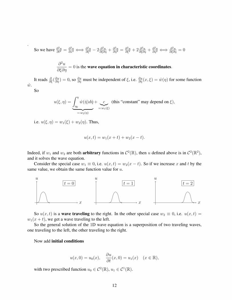
Consider the special case w1 ≡ 0, i.e. u(x, t) = w2(x − t). So if we increase x and t by thesame value, we obtain the same function value for u.
t = 0
x
ut = 1
x
ut = 2
x
u
So u(x, t) is a wave traveling to the right. In the other special case w2 ≡ 0, i.e. u(x, t) =w1(x+ t), we get a wave traveling to the left.
So the general solution of the 1D wave equation is a superposition of two traveling waves,one traveling to the left, the other traveling to the right.
Now add initial conditions
u(x, 0) = u0(x),∂u
∂t(x, 0) = u1(x) (x ∈ R),
with two prescribed function u0 ∈ C2(R), u1 ∈ C1(R).
12

Insert general solution formula into initial conditions:
u(x, 0) = w1(x) + w2(x)!
= u0(x) (x ∈ R),
∂u
∂t(x, 0) =︸︷︷︸
∂u∂t
(x,t)=w′1(x+t)−w′2(x−t)
w′1(x)− w′2(x)!
= u1(x) (x ∈ R)
Integration of the second equation gives
w1(x) + w2(x) =
∫ x
0
u1(s)ds+ c.
Adding and subtracting the two equations gives
w1(x) =1
2(u0(x) +
∫ x
0
u1(s)ds+ c), w2(x) =1
2(u0(x)−
∫ x
0
u1(s)ds− c) (x ∈ R).
So
u(x, t) = w1(x+ t) + w2(x− t) =1
2
[u0(x+ t) + u0(x− t) +
∫ x+t
x−tu1(s)ds
]unique solution of initial value problem for the 1D wave equation, and u ∈ C2(R2) since u0 ∈C2(R), u1 ∈ C1(R).
t
xx− t x+ tx
t
u(x, t) is uniquely determined by the values of u0 and u1 in the interval [x− t, x+ t]. There-fore, this interval is also called dependency interval for (x, t).
Vice versa, the triangle (see picture) is called domain of unique determinacy of the interval[x − t, x + t], because the function values of u0 and u1 inside [x − t, x + t] determine uniquelythe solution u in the triangle.
We can also write
u(x, t) = (Mu1)(x, t) +∂
∂t(Mu0)(x, t),
where
(Mv)(x, t) :=1
2
∫ x+t
x−tv(s)ds;
13
this refers to the higher dimensional case.
So far we solved the so-called Cauchy-problem (for the 1D wave equation), where the initialdata are given on the whole space (here:R) and no boundary conditions are posed.
Now consider the 1D wave equation on a bounded interval [0, l] with additional boundaryconditions
u(0, t) = u(l, t) = 0 (t ≥ 0); see vibrating string example.
So we have the problem∂2u∂t2
= ∂2u∂x2 (0 ≤ x ≤ l, t ≥ 0)
u(0, t) = u(l, t) = 0 (t ≥ 0)
u(x, 0) = u0(x), ∂u∂t
(x, 0) = u1(x) (0 ≤ x ≤ l),
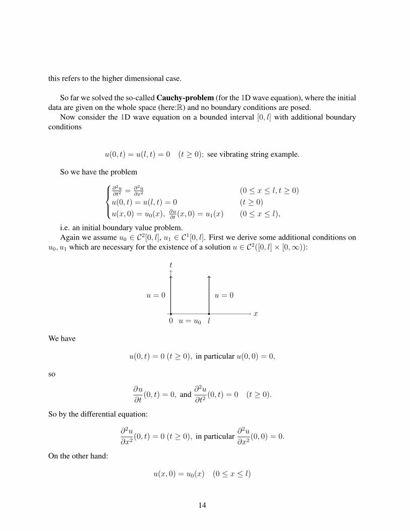
i.e. an initial boundary value problem.Again we assume u0 ∈ C2[0, l], u1 ∈ C1[0, l]. First we derive some additional conditions on
u0, u1 which are necessary for the existence of a solution u ∈ C2([0, l]× [0,∞)):
0 l
u = 0 u = 0
u = u0
x
t
We have
u(0, t) = 0 (t ≥ 0), in particular u(0, 0) = 0,
so
∂u
∂t(0, t) = 0, and
∂2u
∂t2(0, t) = 0 (t ≥ 0).
So by the differential equation:
∂2u
∂x2(0, t) = 0 (t ≥ 0), in particular
∂2u
∂x2(0, 0) = 0.
On the other hand:
u(x, 0) = u0(x) (0 ≤ x ≤ l)
14

so
∂2u
∂x2(x, 0) = u0
′′(x) (0 ≤ x ≤ l), in particular u(0, 0) = u0(0),∂2u
∂x2(0, 0) = u0
′′(0).
So we get the necessary conditions
u0(0) = 0 and u0′′(0) = 0.
Analogously, we obtain
u0(l) = u0′′(l) = 0.
Moreover, from
∂u
∂t(0, t) = 0 (t ≥ 0) (see above), we get in particular
∂u
∂t(0, 0) = 0.
On the other hand
∂u
∂t(x, 0) = u1(x) (0 ≤ x ≤ l), in particular
∂u
∂t(0, 0) = u1(0).
So we get the necessary condition
u1(0) = 0.
Analogously,
u1(l) = 0.
In summary, we get the necessary compatibility conditions
u0(0) = u0(l) = 0, u0′′(0) = u0
′′(l) = 0, u1(0) = u1(l) = 0.
From now on, assume that these compatibility conditions are satisfied.We extend u0 and u1 to the whole of R as followsFirst
ui(−x) := −ui(x) (0 < x ≤ l; i = 0, 1),
which, due to the compatibility conditions, gives
u0 ∈ C2[−l,−l], u1 ∈ C1[−l,−l].
Then,
ui(x+ 2kl) := ui(x) (−l ≤ x ≤ l, k ∈ Z)
gives a 2l- periodic extension to R.
15

This gives functions u0 ∈ C2(R), u1 ∈ C1(R), which both are odd with respect to reflectionat 0 and at l.
Now, define
u(x, t) :=1
2[u0(x, t) + u0(x− t) +
∫ x+t
x−tu1(s)ds]
solution of the Cauchy problem with the extended data u0 and u1.So
∂2u
∂x2(x, t) =
∂2u
∂t2(x, t) for x ∈ R, t ≥ 0, in particular for x ∈ [0, l], t ≥ 0,
and
u(x, 0) = u0(x),∂u
∂t(x, 0) = u1(x) for x ∈ R, in particular for x ∈ [0, l].
We are left to show that also the boundary conditions are satisfied:
u(0, t) =1
2[u0(t) + u0(−t)︸ ︷︷ ︸=0 since u0 is odd at 0
+
∫ t
−tu1(s)ds︸ ︷︷ ︸
=0 since u1 is odd at 0
] = 0,
u(l, t) =1
2[u0(l + t) + u0(l − t)︸ ︷︷ ︸
=0 since u0 is odd at l
+
∫ l+t
l−tu1(s)ds︸ ︷︷ ︸
=0 since u1 is odd at l
] = 0 (t ≥ 0).
So u solves the initial boundary value problem.
2.2 The wave equation in R3
Here we only consider the Cauchy problem. The problem therefore reads:∂2u
∂t2= ∆u (x ∈ R3, t ≥ 0)
u(x, 0) = u0(x),∂u
∂t(x, 0) = u1(x) (x ∈ R3)
with given functions u0, u1 : R3 → R.Define the spherical mean value for any function v ∈ C(R3):
(Mv)(x, r) :=1
4π
∫S
v(x+ ry)dσ(y) (x ∈ R3 r ≥ 0)
where S := y ∈ R3 : |y| = 1 is the unit sphere in R3, dσ(y) is the surface measure on S.The representation in polar coordinates reads:
(Mv)(x, r) =1
4π
∫ 2π
0
(∫ π
0
v(x1 + r cosϕ sin θ, x2 + r sinϕ sin θ, x3 + r cos θ) sin θdθ
)dϕ
16

Theorem 2.1. Let v ∈ C2(R3). Then, for all x ∈ R3 and r > 0:∫y∈R3:|y|≤r
(∆v)(x+ y)dy = 4πr2 ∂
∂r(Mv)(x, r).
Corollary 2.2. Let v ∈ C2(R3) and ∆v = 0 on R3 (i.e. v is harmonic on R3, i.e. it solves theLaplace equation). Then,
(Mv)(x, r) = v(x) (x ∈ R3 r ≥ 0).
mean value property of harmonic functions.
Proof of Theorem 2.1. Let
I :=
∫|y|≤r
(∆v)(x+ y)dy =
∫|y|≤r
(div(grad v)) (x+ y)dy
Substitute y = ry, then dy = r3dy and
I = r3
∫|y|≤1
(div(grad v)) (x+ ry)dy.
Let w(y) := v(x+ ry), then
(gradw)(y) = r(grad v)(x+ ry) and (div(gradw)(y)) = r2 (div(grad v)) (x+ ry).
Therefore,
I = r
∫|y|≤1
(div(gradw)) (y)dy
Gauss Theorem= r
∫S
(gradw)(y) · ν(y)︸︷︷︸=y
dσ(y)
= r2
∫S
(grad v)(x+ ry) · y︸ ︷︷ ︸Chain rule
= ∂∂r
[v(x+ry)]
dσ(y)
= r2
∫S
∂
∂r[v(x+ ry)]dσ(y)
v∈C2(R3)= r2 ∂
∂r
∫S
v(x+ ry)dσ(y)︸ ︷︷ ︸= 4π(Mv)(x,r)
= 4πr2 ∂
∂r(Mv)(x, r)
17

Proof of Corollary 2.2. Since ∆v ≡ 0, Theorem 2.1 gives ∂∂r
(Mv)(x, r) = 0, i.e. (Mv)(x, r) isconstant with respect to r.
So
(Mv)(x, r) = (Mv)(x, 0) =1
4π
∫S
v(x+ 0y)︸ ︷︷ ︸= v(x)
dσ(y)
= v(x) · 1
4π
∫S
dσ(y)︸ ︷︷ ︸= 4π
= v(x)
Lemma 2.3. For v ∈ C2(R3) we have
∂
∂r
[∫|y|≤r
v(x+ y)dy
]= 4πr2(Mv)(x, r) (x ∈ R3 r ≥ 0)
Proof.∫|y|≤r
v(x+ y)dy =
=
∫ r
0
[∫ 2π
0
(∫ π
0
v(x1 + ρ cosϕ sin θ, x2 + ρ sinϕ sin θ, x3 + ρ cos θ) sin θdθ
)dϕ
]ρ2dρ
Hence,
∂
∂r
∫|y|≤r
v(x+ y)dy =
= r2
∫ 2π
0
(∫ π
0
v(x1 + r cosϕ sin θ, x2 + r sinϕ sin θ, x3 + r cos θ) sin θdθ
)dϕ = 4πr2(Mv)(x, r)
Lemma 2.4. Let u ∈ C2(R3 × [0,∞)) be a solution of the Cauchy problem
∂2u
∂t2= ∆u (x ∈ R3 t ≥ 0), u(x, 0) = u0(x),
∂u
∂t(x, 0) = u1(x) (x ∈ R3).
Let w(x, r, t) := r(Mu)(x, r, t), where the mean value operator in applied for each fixed t,more precisely w(x, r, t) := [M(u(·, t))](x, r). Then,
∂2w
∂t2(x, r, t) =
∂2w
∂r2(x, r, t) (x ∈ R3, r > 0, t ≥ 0),
w(x, r, 0) = r(Mu0)(x, r),∂w
∂t(x, r, 0) = r(Mu1)(x, r) (x ∈ R3, r > 0).
18

Proof. By Theorem 2.1:
4πr2 ∂
∂r(Mu)(x, r, t) =
∫|y|≤r
(∆u)(x+ y, t)dyu solution
=
∫|y|≤r
∂2u
∂t2(x+ y, t)dy
u C2-smooth, |y|≤r compact=
∂2
∂t2
∫|y|≤r
u(x+ y, t)dy.
Take derivative with respect to r:
8πr∂
∂r(Mu)(x, r, t) + 4πr2 ∂
2
∂r2(Mu)(x, r, t) =
∂2
∂t2∂
∂r
∫|y|≤r
u(x+ y, t)dy
Lemma 2.3=
∂2
∂t24πr2(Mu)(x, r, t) = 4πr2 ∂
2
∂t2(Mu)(x, r, t).
So
2∂
∂r(Mu)(x, r, t) + r
∂2
∂r2(Mu)(x, r, t) = r
∂2
∂t2(Mu)(x, r, t),
i.e.
∂2
∂r2[r(Mu)(x, r, t)︸ ︷︷ ︸
=w(x,r,t)
] =∂2
∂t2[r(Mu)(x, r, t)︸ ︷︷ ︸
=w(x,r,t)
]
Moreover,
w(x, r, 0) = r(Mu)(x, r, 0) = r(M(u(·, 0︸ ︷︷ ︸=u0
)))(x, r) = r(Mu0)(x, r)
and
∂w
∂t(x, r, 0) = r
∂
∂t(Mu)(x, r, t)
∣∣∣∣t=0
= r
(M∂u
∂t
)(x, r, t)
∣∣∣∣t=0
= r
(M
(∂u
∂t(·, 0)︸ ︷︷ ︸
=u1
))(x, r) = r(Mu1)(x, r).
Theorem 2.5. The Cauchy problem
∂2u
∂t2= ∆u (x ∈ R3 t ≥ 0), u(x, 0) = u0(x),
∂u
∂t(x, 0) = u1(x) (x ∈ R3),
where u0 ∈ C3(R3), u1 ∈ C2(R3), has a unique solution u ∈ C2(R3 × [0,∞)); it is given by
u(x, t) =∂
∂t[t(Mu0)(x, t)] + t(Mu1)(x, t).
(Compare the 1D formula)
19

Proof. Let u ∈ C2(R3 × [0,∞)) be a solution of the Cauchy problem, and let w as in Lemma2.4, i.e.
w(x, r, t) = r(Mu)(x, r, t).
Then
∂w
∂r(x, r, t) = (Mu)(x, r, t) + r
∂
∂r(Mu)(x, r, t)
=1
4π
∫S
u(x+ ry, t)dσ(y) +r
4π
∫S
(∇u)(x+ ry, t) · ydσ(y)
has a limit as r → 0. Extend w by odd reflection to (−∞, 0):
w(x, r, t) := −w(x,−r, t) for r < 0 (and x ∈ R3, t ≥ 0).
Then
∂w
∂r(x, r, t) =
∂w
∂r(x,−r, t),
∂2w
∂r2(x, r, t) = −∂
2w
∂r2(x,−r, t) Lemma 2.4
= −∂2w
∂t2(x,−r, t) =
∂2w
∂t2(x, r, t) (r < 0, x ∈ R3, t ≥ 0).
Since w(x, 0, t) = 0 and ∂w∂r
(x, r, 0) has a limit as r → 0, we have a C1-transition at r = 0.Moreover, the wave equation for w is satisfied also for r < 0.
Furthermore, since w(x, 0, t) = 0, we have ∂2w∂t2
(x, 0, t) = 0, so by taking the limit r → 0 inthe wave equation for w we obtain ∂2w
∂r2 (x, 0, t) = 0.This gives a C2-transition at r = 0. So the extended w is in C2(R3 × R × [0,∞)), and it
satisfies the 1D wave equation for all r ∈ R.Furthermore, for r < 0:
w(x, r, 0) = −w(x,−r, 0) = −(−r)(Mu0)(x,−r) = r(Mu0)(x,−r)
= r1
4π
∫S
u0(x− ry)dσ(y)y=−y, dσ(y)=dσ(y)
=r
4π
∫S
u0(x+ ry)dσ(y) = r(Mu0)(x, r)
and
∂w
∂t(x, r, 0) = −∂w
∂t(x,−r, 0) = −(−r)(Mu1)(x,−r) = r(Mu1)(x,−r) = r(Mu1)(x, r).
So also the initial conditions extend to all r ∈ R. Now the solution formula for the 1D Cauchyproblem gives
w(x, r, t) =1
2
[(r + t)(Mu0)(x, r + t) + (r − t)(Mu0)(x, r − t) +
∫ r+t
r−ts(Mu1)(x, s)ds
].
20

So
∂w
∂r(x, r, t) =
1
2[(Mu0)(x, r + t) + (r + t)
∂
∂r[(Mu0)(x, r + t)]︸ ︷︷ ︸
= ∂∂t
[... ]
+(Mu0)(x, r − t)
+ (r − t) ∂∂r
[(Mu0)(x, r − t)]︸ ︷︷ ︸=− ∂
∂t[... ]
+(r + t)(Mu1)(x, r + t)− (r − t)(Mu1)(x, r − t)]
Evaluate at r = 0:
∂w
∂r(x, 0, t) =
1
2
[(Mu0)(x, t) + (Mu0)(x,−t)︸ ︷︷ ︸
=(Mu0)(x,t)
+t∂
∂t(Mu0)(x, t) + t
∂
∂t[(Mu0)(x,−t)]︸ ︷︷ ︸
=(Mu0)(x,t)
+ t(Mu1)(x, t) + t (Mu1)(x,−t)︸ ︷︷ ︸=(Mu1)(x,t)
]
= (Mu0)(x, t) + t∂
∂t[(Mu0)(x, t)] + t(Mu1)(x, t)
=∂
∂t[t(Mu0)(x, t)] + t(Mu1)(x, t) (12)
On the other hand, since w(x, r, t) = r(Mu)(x, r, t) :
∂w
∂r(x, r, t) = (Mu)(x, r, t) + r
∂
∂r[(Mu)(x, r, t)]︸ ︷︷ ︸
bounded as r→0, since u is C2−smooth.
,
so
∂w
∂r(x, 0, t) = (Mu)(x, 0, t) =
1
4π
∫S
u(x+ 0y, t)dσ(y) = u(x, t)1
4π
∫S
dσ(y) = u(x, t)
Comparing with (12) gives
u(x, t) =∂
∂t[t(Mu0)(x, t)] + t(Mu1)(x, t).
Hence, u has the asserted form, and also uniqueness is proved.
We are left to show: u defined by this formula is indeed a solution. First, since u0 ∈ C3(R3),u1 ∈ C2(R3), we have u ∈ C2(R3 × [0,∞)).
Moreover,
∂u
∂t(x, t) = 2
∂
∂t[(Mu0)(x, t)] + t
∂2
∂t2[(Mu0)(x, t)] + [(Mu1)(x, t)] + t
∂
∂t[(Mu1)(x, t)].
21

So
u(x, 0) = (Mu0)(x, 0) +
t∂
∂t[(Mu0)(x, t)]
∣∣∣∣t=0
= (Mu0)(x, 0)
=1
4π
∫S
u0(x+ 0y)dσ(y) = u0(x).
and
∂u
∂t(x, 0) = 2
∂
∂t[(Mu0)(x, t)]
∣∣∣∣t=0
+ (Mu1)(x, 0)︸ ︷︷ ︸=u1(x)
,
and
∂
∂t[(Mu0)(x, t)]
∣∣∣∣t=0
=∂
∂t
1
4π
∫S
u0(x+ ty)dσ(y)
∣∣∣∣t=0
=1
4π
∫S
(∇u0)(x+ ty) · ydσ(y)
∣∣∣∣t=0
=1
4π
∫S
(∇u0)(x) · y︸ ︷︷ ︸=∑3i=1
∂u0∂xi
(x)·yi
dσ(y) =1
4π
3∑i=1
∂u0
∂xi(x)
∫S
yi︸︷︷︸=νi(y)
dσ(y)
Gauss=
1
4π
3∑i=1
∂u0
∂xi(x)
∫|y|≥1
∂1
∂xidx
So indeed ∂u∂t
(x, 0) = u1(x). We are left to show: u satisfies the wave equation. The form of ushows that it is sufficient to prove: For every v ∈ C2(R3), the function w(x, t) := t(Mv)(x, t)satisfies the wave equation.
[Note: If z ∈ C3(R3 × [0,∞)) solves the wave equation ∂2z∂t2
= ∆z, then taking the timederivative we see that also ∂z
∂tdoes so.]
Indeed:
∂w
∂t(x, t) = (Mv)(x, t) + t
∂
∂t[(Mv)(x, t)] ,
∂2w
∂t2(x, t) = 2
∂
∂t[(Mv)(x, t)] + t
∂2
∂t2[(Mv)(x, t)]
Moreover, by Theorem 2.1 :
∂
∂t[(Mv)(x, t)] =
1
4πt2
∫|y|≤t
(∆v)(x+ y)dy.
So
∂2
∂t2[(Mv)(x, t)] = − 2
4πt3
∫|y|≤t
(∆v)(x+ y)dy +1
4πt2∂
∂t
∫|y|≤t
(∆v)(x+ y)dy︸ ︷︷ ︸Lemma 2.3
=4πt2(M(∆v))(x,t)
22

Thus,
∂2w
∂t2(x, t) = 2
∂
∂t[(Mv)(x, t)] + t
∂2
∂t2[(Mv)(x, t)] = t(M(∆v))(x, t)
=t
4π
∫S
(∆v)(x+ ty)dσ(y)
∆v continuous, S compact=
t
4π∆
(∫S
v(·+ ty)dσ(y)
)= t(∆(Mv))(x, t) = ∆[t(Mv)(·, t)] = (∆w)(x, t).
2.3 The wave equation in R2
(vibrating membrane, water waves). Again, we only consider the Cauchy problem. Hence, theequation to be studied is
∂2u
∂t2= ∆u (x ∈ R2 t ≥ 0), u(x, 0) = u0(x),
∂u
∂t(x, 0) = u1(x) (x ∈ R2) (Cauchy problem)
with u0 ∈ C3(R2), u1 ∈ C2(R2).Solution using Hadamard’s descent method: Suppose u ∈ C2(R2 × [0,∞)) is a solution.
Define
w(x1, x2, x3, t) := u(x1, x2, t) (x = (x1, x2, x3) ∈ R3, t ≥ 0).
Obviously,
∂2w
∂t2(x1, x2, x3, t) =
∂2u
∂t2(x1, x2, t) = (∆u)(x1, x2, t) =
2∑i=1
∂2u
∂xi2(x1, x2, t)
=3∑i=1
∂2w
∂xi2(x1, x2, x3, t) = (∆w)(x1, x2, x3, t),
i.e. w is a solution of the 3D wave equation. Moreover, w satisfies the initial condition
w(x1, x2, x3, 0) = u0(x1, x2)︸ ︷︷ ︸=:w0(x1,x2,x3)
,∂w
∂t(x1, x2, x3, 0) =
∂u
∂t(x1, x2, 0) = u1(x1, x2)︸ ︷︷ ︸
=:w1(x1,x2,x3)
.
By Theorem 2.5 we get
w(x1, x2, x3, t) =∂
∂t[t(Mw0)(x1, x2, x3, t)] + t(Mw1)(x1, x2, x3, t).
23

Lemma 2.6. Let v ∈ C2(R2), z(x1, x2, x3) := v(x1, x2) for (x1, x2, x3) ∈ R3. Then,
(Mz)(x1, x2, x3, r) =1
2π
∫|y|≤1, y∈R2
v(x1 + ry1, x2 + ry2)√1− |y|2
dy1dy2.
Proof.
(Mz)(x1, x2, x3, r) =1
4π
∫S⊂R3
z(x1 + ry1, x2 + ry2, x3 + ry3)︸ ︷︷ ︸=v(x1+ry1,x2+ry2)
dσ(y)
=1
4π
∫ π
0
(∫ 2π
0
v(x1 + r cosϕ sin θ, x2 + r sinϕ sin θ)dϕ
)sin θdθ
=1
2π
∫ π2
0
(∫ 2π
0
v(x1 + r cosϕ sin θ, x2 + r sinϕ sin θ)dϕ
)sin θdθ
ρ=sin θ, dρ=cos θdθ=√
1−sin2 θdθ=√
1−ρ2dθ=
1
2π
∫ 1
0
(∫ 2π
0
v(x1 + rρ cosϕ, x2 + rρ sinϕ)dϕ
)ρ√
1− ρ2dρ
Now consider 2D polar coordinates:
y1 = ρ cosϕ, y2 = ρ sinϕ, dy1dy2 = ρdρdϕ
So the calculation continuous:
(Mz)(x1, x2, x3, r) =1
2π
∫|y|≤1, y∈R2
v(x1 + ry1, x2 + ry2)√1− |y|2
dy1dy2 (note |y2| = y21 + y2
2 = ρ2)
So we obtain for u(x1, x2, t) = w(x1, x2, x3, t):
u(x1, x2, t) =∂
∂t
[t
1
2π
∫|y|≤1
u0(x+ ty)√1− |y|2
dy
]+ t
1
2π
∫|y|≤1
u1(x+ ty)√1− |y|2
dy,
which is the desired solution formula of the Cauchy problem for the 2D wave equation.We omit here the proof that the formula actually gives a solution to the Cauchy problem, this
proof can be done by again going back to w and the 3D result Theorem 2.5.In the solution formula, we can transform y = ty, so dy = t2dy, thus
u(x, t) =∂
∂t
1
2πt
∫|y|≤t
u0(x+ y)√1− |y|2
t2
dy
+1
2πt
∫|y|≤t
u1(x+ y)√1− |y|2
t2
dy,
which implies, renaming y as y again,
u(x, t) =1
2π
∂
∂t
[∫|y|≤t
u0(x+ y)√t2 − |y|2
dy
]+
1
2π
∫|y|≤t
u1(x+ y)√t2 − |y|2
dy.
24
The dependency of the solution to the wave equation on the dimension.In 3D (after transformation y = ty, then renaming y as y again):
u(x, t) =∂
∂t
[1
4πt
∫|y|=t
u0(x+ y)dσ(y)
]+
1
4πt
∫|y|=t
u1(x+ y)dσ(y).
In 2D: See above, in 1D:
u(x, t) =1
2
[u0(x+ t) + u0(x− t) +
∫ x+t
x−tu1(s)ds
]Now consider the situation when u0 and u1 have compact support, i.e. they vanish outside somecompact set.
Then in 3D, we have for fixed x ∈ R3: The “signals” u0 and u1 are received with sharp startand sharp end.
In 2D, the signals are received with a sharp start, but not with a sharp end. However, itdecreases, as t→∞, like 1
t.
In 1D, the signal u0 has a sharp start and sharp end; the signal u1 has a sharp start, but noend, and it does not decrease as t→∞ (in general).
2.4 The inhomogeneous wave equation
∂2u
∂t2−∆u = w(x, t) (x ∈ Rn t ≥ 0)
u(x, 0) = u0(x),∂u
∂t(x, 0) = u1(x) (x ∈ Rn),
where u0, u1, w are given.(Example: wave equation for electro-magnetic waves, where w ∼ current density, charge
density).Assume u0 ∈ C3(Rn) (C2(R) if n = 1), u1 ∈ C2(Rn) (C1(R) if n = 1) andw ∈ C2(Rn × [0,∞)) (C1(Rn × [0,∞)) if n = 1). These smoothness assumption can be
weakened. In particular smoothness with respect to time t is not needed.As in all linear problems, the general solution of the inhomogeneous differential equation is
given as the general solution of the homogeneous differential equation + one special solution ofthe inhomogeneous differential equation.
For finding a special solution to the inhomogeneous differential equation, we use Duhamel’smethod: Recall the variational-of-constants-formula∫ t
0
Φ(t)Φ(s)−1︸ ︷︷ ︸Φ(t−s) if the equation is autonomous.
w(s)ds
25

from ODE theory. Correspondingly, we now make the ansatz
v(x, t) =
∫ t
0
V (x, t− s, s)ds
for a special solution v(x, t). Here, V ∈ C2(Rn × [0,∞)× [0,∞) has to be found.Since [0, t] is compact and v ∈ C2:
(∆v)(x, t) =
∫ t
0
(∆V )(x, t− s, s)ds,
∂v
∂t(x, t) = V (x, 0, t) +
∫ t
0
(∂n+1V )(x, t− s, s)ds,
∂2v
∂t2(x, t) = (∂n+2V )(x, 0, t) + (∂n+1V )(x, 0, t) +
∫ t
0
(∂2n+1V )(x, t− s, s)ds.
So∂2v
∂t2(x, t)− (∆v)(x, t) = (∂n+2V )(x, 0, t) + (∂n+1V )(x, 0, t)
+
∫ t
0
[(∂2n+1V )−∆V ](x, t− s, s)ds !
= w(x, t)
Therefore, we require [(∂2n+1V )︸ ︷︷ ︸= ∂2V∂t2
−∆V ](x, t, s) = 0 for all x ∈ Rn, t ≥ 0, s ≥ 0, and
moreover, V (x, 0, s) = 0 (x ∈ Rn, s ≥ 0), which implies (∂n+2V )(x, 0, s) = 0 (s ≥ 0), and(∂n+1V )︸ ︷︷ ︸
= ∂V∂t
(x, 0, s) = w(x, s) (x ∈ Rn, s ≥ 0).
Then, ∂2V∂t2−∆v = w as desired, and moreover, v(x, 0) = 0, ∂v
∂t(x, 0) = 0 (x ∈ Rn).
Then, u(x, t) := u(x, t) + v(x, t) is the solution of the given problem, where u solves
∂2u
∂t2−∆u = 0 (x ∈ Rn t ≥ 0),
u(x, 0) = u0(x),∂u
∂t(x, 0) = u1(x) (x ∈ Rn),
i.e. if, for example, n = 3:
u(x, t) =∂
∂t[t(Mu0)(x, t)] + t(Mu1)(x, t).
The remaining task is to solve the parameter dependent Cauchy problem for V (x, t, s):(∂2V
∂t2−∆V
)(x, t, s) = 0 (x ∈ Rn, t ≥ 0, s ≥ 0),
V (x, 0, s) = 0,∂V
∂t(x, 0, s) = w(x, s) (x ∈ Rn, s ≥ 0).
26
For n = 1: exercises.For n = 3:
V (x, t, s) =∂
∂t[t(M0)(. . . )] + t[M(w(·, s))](x, t) =
t
4π
∫S
w(x+ ty, s)dσ(y)
Hence
v(x, t) =
∫ t
0
V (x, t− s, s)ds =1
4π
∫ t
0
(t− s)(∫
S
w(x+ (t− s)y, s)dσ(y)
)ds
τ=t−s, dτ=−ds=
1
4π
∫ t
0
τ
(∫S
w(x+ τy, t− τ)dσ(y)
)dτ
η=τy, dσ(η)=τ2dσ(y)=
1
4π
∫ t
0
1
τ
(∫|η|=τ
w(x+ η, t− τ)dσ(η)
)dτ
Cavalieri=
1
4π
∫|η|≤t (ball)
w(x+ η, t− |η|)|η|
dη “retarded potential”
So, in 3D, the solution to the given inhomogeneous problem reads
u(x, t) =∂
∂t[t(Mu0)(x, t)] + t(Mu1)(x, t) +
1
4π
∫|η|≤t
w(x+ η, t− |η|)|η|
dη
2.5 Separation of variablesExample 2.7. Vibrating String (without loss of generality of length l = π):
∂2u
∂t2=∂2u
∂x2(0 ≤ x ≤ π, t ≥ 0), u(0, t) = u(π, t) = 0 (t ≥ 0);
u(x, 0) = u0(x),∂u
∂t(x, 0) = u1(x) (0 ≤ x ≤ π).
We make the separation of variables ansatz
u(x, t) = v(x)g(t).
Insert into differential equation:
v(x)g′′(t) = v′′(x)g(t) (0 ≤ x ≤ π, t ≥ 0)
If v(x) 6= 0, g(t) 6= 0:
g′′(t)
g(t)=v′′(x)
v(x)(0 ≤ x ≤ π, t ≥ 0).
27

The left-hand side depends only on t, the right-hand side only on x, so both must be constant.Thus,
g′′(t)
g(t)= −λ (t ≥ 0),
v′′(x)
v(x)= −λ (0 ≤ x ≤ π).
for some constant λ ∈ C. The boundary conditions become
v(0)g(t) = v(π)g(t) = 0 (t ≥ 0).
So for v we obtain the ODE boundary value problem
−v′′(x) = λv(x) (0 ≤ x ≤ π), v(0) = v(π) = 0.
We are only interested in solutions v 6= 0. So the problem to be solved is an eigenvalue problem:We are looking for λ ∈ C such that a non-trivial solution v exists. Here, we can solve thiseigenvalue problem in closed form: The general solution of the differential equation reads
v(x) =
c1 exp(
√−λx) + c2 exp(−
√−λx), if λ 6= 0
c1 + c2x, if λ = 0
with arbitrary constants c1, c2 ∈ C.
Here ±√−λ denote the two complex roots of −λ.
For λ = 0, the boundary conditions v(0) = v(π) = 0 imply v ≡ 0. So λ = 0 is no eigenvalue.Thus, let λ 6= 0. Since v(0) = 0, we have c2 = −c1, and thus
v(x) = c1[exp(√−λx)− exp(−
√−λx)] = c12i
exp(i√λx)− exp(−i
√λx)
2i= c12i sin(
√λx)
The second boundary conditions v(π) = 0 implies (since we want to avoid v ≡ 0) sin(√λπ) = 0,
so we must have√λπ = nπ for some n ∈ N, i.e.
λ = n2 for some n ∈ N.
The nontrivial function v associated with the eigenvalue λ = λn = n2 is
vn(x) = sin(nx) (0 ≤ x ≤ π),
up to a multiplicative constant. vn is called eigenfunction associated with the eigenvalueλn = n2.
The function g therefore must satisfy
−g′′(t) = n2g(t) (t ≥ 0), i.e. g(t) = a cos(nt) + b sin(nt) (t ≥ 0).
Thus
u(x, t) = sin(nx)[an cos(nt) + bn sin(nt)]
is our “separated variables solution”. (an, bn ∈ C arbitrary constants; n ∈ N)
28

Inserting this u into the differential equation and boundary conditions shows: u indeed solvesthese, even though the intermediate assumption v(x) 6= 0, g(t) 6= 0 is violated.
Due to linearity, also
u(x, t) =∞∑n=1
sin(nx)[an cos(nt) + bn sin(nt)],
provided the series converges in an appropriate sense, allowing for example differentiation insidethe series. Then
u(x, 0) =∞∑n=1
an sin(nx) and∂u
∂t(x, 0) =
∞∑n=1
nbn sin(nx).
So we want to determine an, bn such that
u0(x) =∞∑n=1
an sin(nx), u1(x) =∞∑n=1
nbn sin(nx),
in order to satisfy the initial conditions. The theory of Fourier series tells:The two identities hold for
an =2
π
∫ π
0
u0(s) sin(ns)ds, bn =2
πn
∫ π
0
u1(s) sin(ns)ds,
and the convergence of the two Fourier series is uniform if u0, u1 ∈ C1[0, π] andu0(0) = u0(π) = u1(0) = u1(π) = 0.Indeed, if we slightly strengthen the smoothness of u0, requiring u0 ∈ C2[0, π], the above
series
u(x, t) =∞∑n=1
sin(nx)[an cos(nt) + bn sin(nt)],
with an, bn given as above, is the solution of our initial value problem.Returning to the vibrating string application: n = 1 gives the basic tone, n = 2 the first
harmonic, n = 3 second harmonic, . . . , and the true vibration (“sound”) of the string is a super-position of these harmonics.
Example 2.8. Vibrating membrane
∂2u
∂t2= ∆u in Ω× (0,∞); u = 0 on ∂Ω× (0,∞);
u(x, 0) = u0(x),∂u
∂t(x, 0) = u1(x) (x ∈ Ω), Ω ⊂ R2 domain.
29
In the following, we write (x, y) instead of x = (x1, x2). Make a separation ansatz again:
u(x, y, t) = v(x, y)g(t)
Inserting into differential equation and boundary conditions gives, as before,
v(x, y)g′′(t) = (∆v)(x, y)g(t),
i.e. if v(x, y) 6= 0, g(t) 6= 0:
(∆v)(x, y)
v(x, y)=g′′(t)
g(t)!
= −λ
and
v(x, y)g(t) = 0 for (x, y) ∈ ∂Ω, t ≥ 0.
So we get −(∆v)(x, y) = λv(x, y) ((x, y) ∈ Ω),
v(x, y) = 0 ((x, y) ∈ ∂Ω),
and
g′′(t) + λg(t) = 0 (t ≥ 0).
All eigenvalues λ of this problem must be positive:Let λ ∈ C be an eigenvalue, v an associated eigenfunction, then
λ
∫Ω
|v|2︸︷︷︸=vv
dxdy =
∫Ω
(−∆v)(x, y)v(x, y)dxdyGreen= −
∫∂Ω
∂v
∂νv︸︷︷︸
=0
dσ +
∫Ω
| grad v|2dxdy,
so
λ =
∫Ω| grad v|2dxdy∫
Ω|v|2dxdy
> 0.
So there exists ω > 0 such that λ = ω2. So for g we obtain g(t) = a cos(ωt)+b sin(ωt); a, b ∈ Carbitrary, and finally the separation solution
u(x, y, t) = v(x, y)[an cos(ωt) + bn sin(ωt)].
Now we use the expansion theorem, which tells that every function with suitable properties canbe expanded in a series of eigenfunctions of
−∆v = λv in Ω,
v = 0 on ∂Ω
30

There exists a sequence (λn)n∈N of eigenvalues converging to +∞, with associated eigen-functions vn which are orthonormal with respect to
< u, v >=
∫Ω
u(x)v(x)dx, i.e. < vn, vm >= δnm,
and complete in the sense that every (sufficiently smooth) function ϕ can be written as
ϕ(x, y) =∞∑n=1
< ϕ, vn > vn(x, y)
(for example, if ϕ ∈ L2(Ω), then the series converges in L2(Ω)). So from the separation solutionswe therefore obtain the more general solution
u(x, y, t) =∞∑n=1
vn(x, y)[an cos(ωnt) + bn sin(ωnt)], ωn2 = λn
The initial conditions require
u0 =∞∑n=1
anvn, u1 =∞∑n=1
ωnbnvn.
The expansion theorem tells that such an expansion for u0 and u1 is indeed at hand if u0, u1 aresufficiently smooth and satisfy the boundary conditions, namely we have
an =< u0, vn >, bn =1
ωn< u1, vn > .
Special cases:
a) Rectangular membrane
Ω = (x, y) ∈ R2 : 0 ≤ x ≤ a, 0 ≤ y ≤ b
So our eigenvalue problem reads −∆v = λv in Ω,
v = 0 on ∂Ω
can be attacked by separation of variables again: Make the ansatz
v(x, y) = w1(x)w2(y)
Insert into differential equation:
−w′′1(x)w2(y)− w1(x)w′′2(y) = λw1(x)w2(y)
31

Assume (again) that w1(x) 6= 0, w2(y) 6= 0 and divide:
−w′′1(x)
w1(x)− w′′2(y)
w2(y)= λ, i.e.
w′′1(x)
w1(x)+ λ = −w
′′2(y)
w2(y)
As before we conclude that both sides are constant =: λ(2) :
w′′1(x)
w1(x)+ λ = λ(2), −w
′′2(y)
w2(y)= λ(2),
i.e. for λ(1) := λ− λ(2):
−w′′1(x) = λ(1)w1(x) (0 ≤ x ≤ a), −w′′2(y) = λ(2)w2(y) (0 ≤ y ≤ b),
and λ(1) + λ(2) = λ.The boundary condition requires w1(x)w2(y) = 0 on ∂Ω, which means (becausew1(x) 6= 0, w2(y) 6= 0):
w1(0) = w1(a) = 0, w2(0) = w1(b) = 0.
So we get the two eigenvalue problems−w′′1(x) = λ(1)w1(x) (0 ≤ x ≤ a)
w1(0) = w1(a) = 0
and
−w′′2(y) = λ(2)w2(y) (0 ≤ y ≤ a)
w2(0) = w2(b) = 0
and λ(1) + λ(2) = λ.The eigenvalues and eigenfunctions are
w1(x) = sin(nπax), λ(1) = n2
(πa
)2
, w2(y) = sin(mπby), λ(2) = m2
(πb
)2
.
So for 2D problem we get the eigenvalues and eigenfunctions
λm,n = π2
(n2
a2+m2
b2
), vn,m(x, y) = sin
(nπax)
sin(mπby).
b) Circular membrane (without loss of generality with radius 1):
Ω = (x, y) ∈ R2 : x2 + y2 < 1
The differential equation −∆v = λv has, written in polar coordinates, the form
−∂2v
∂r2− 1
r
∂v
∂r− 1
r2
∂2v
∂ϕ2= λv
(see exercise), and the boundary condition becomes
v(1, ϕ) = 0 (0 ≤ ϕ ≤ 2π).
32

Try separation of variables again: v(r, ϕ) = f(r)h(ϕ). Insert into the differential equation:
−f ′′(r)h(ϕ)− 1
rf ′(r)h(ϕ)− 1
r2f(r)h′′(ϕ) = λf(r)h(ϕ).
Again assuming f(r) 6= 0, h(ϕ) 6= 0, we obtain upon multiplying by r2
f(r)h(ϕ):
−r2[f ′′(r) + 1rf ′(r) + λf(r)]
f(r)=h′′(ϕ)
h(ϕ)=: −c
So h′′(ϕ) = −ch(ϕ), and h must be 2π-periodic (otherwise v would not be smooth in the (x, y)-coordinates), i.e. h(0) = h(2π), h′(0) = h′(2π). From this we conclude
h(ϕ) =
α cos(
√cϕ) + β sin(
√cϕ) if c 6= 0
α + βϕ if c = 0
,
√c ∈ C a complex roof of c. Periodicity implies
√c = n ∈ N0, i.e.
c = n2 and h(ϕ) = α cos(nϕ) + β sin(nϕ).
So for f we have
r2f ′′(r) + rf ′(r) + (r2λ− n2)f(r) = 0.
In addition, f has to be “regular” at 0, and it has to satisfy f(1) = 0 (because v = 0 on ∂Ω).The transformation (note: λ > 0)
ρ = r√λ, y(ρ) := f(r) = f
(ρ√λ
)gives
dy(ρ)
dρ=
1√λf ′(r),
d2y(ρ)
dρ2=
1
λf ′′(r).
So the differential equation for f (after division by r2λ) turns into
d2y(ρ)
dρ2+
1
rλ·√λ︸ ︷︷ ︸
= 1ρ
dy(ρ)
dρ+ (1− n2
r2λ︸︷︷︸=n2
ρ2
)y(ρ) = 0,
i.e.
d2y
dρ2+
1
ρ
dy
dρ+
(1− n2
ρ2
)y = 0 Bessel’s differential equation.
33
Its solutions are the Bessel functions (of the first kind: regular at 0, of the second kind: singularat 0). Since f (and thus y) has to be regular at 0, we have to take the Bessel functions of the firstkind
y(ρ) = Jn(ρ)
Jn has infinitely many zeros kn,m (m ∈ N); here without proof. Since f(1) = 0, we needy(√λ) = 0, i.e.
√λ = kn,m for some m ∈ N, i.e.
λ = k2n,m
The associated eigenfunctions vm,n are given byv0,m(r, ϕ) = J0(k0,mr), λ0,m = k2
0,m
v(1)n,m(r, ϕ) = Jn(kn,mr) cos(nϕ), λ
(1)n,m = k2
n,m
v(2)n,m(r, ϕ) = Jn(kn,mr) sin(nϕ), λ
(2)n,m = k2
n,m
Example 2.9. The Schrodinger equation for the hydrogen atom.
i∂Φ
∂t= ∆Φ− V (x)Φ time dependent Schrodinger equation,
V : R3 → R is the potential, and the solution Φ is the wave function of the underlying quantummechanical system. Separation of space and time Φ(x, t) = u(x)g(t) leads to the eigenvalueproblem
−∆u+ V (x)u = λu (x ∈ R3).
For the hydrogen atom, the potential V reads V (x) = − c|x| . This is the Coulomb potential,
which describes the electrical attraction between nucleus (one proton), sitting in 0, and electron.We use spherical coordinates again. In spherical coordinates, the Laplace operator (in 3D)
reads
(∆u)(r, θ, ϕ) =1
r
∂2
∂r2(ru)︸ ︷︷ ︸
= ∂2u∂r2
+ 2r∂u∂r
= 1r2
∂∂r (r2 ∂u
∂r )
+1
r2 sin θ
∂
∂θ
(sin θ
∂u
∂θ
)+
1
r2 sin2 θ
∂2u
∂ϕ2
So the eigenvalue problem reads
1
r
∂2
∂r2(ru) +
1
r2 sin θ
∂
∂θ
(sin θ
∂u
∂θ
)+
1
r2 sin2 θ
∂2u
∂ϕ2+c
ru+ λu = 0.
Separation ansatz u(r, θ, ϕ) = v(r)Y (θ, ϕ):
1
r
∂2
∂r2(rv) · Y +
1
r2 sin θ
∂
∂θ
(sin θ
∂Y
∂θ
)· v +
1
r2 sin2 θ
∂2Y
∂ϕ2· v +
(cr
+ λ)vY = 0
34
Multiplying by r2
v·Y
r ∂2
∂r2 (rv)
v+ (cr + λr2)︸ ︷︷ ︸
= constant =: l(l+1)
+
1sin θ
∂∂θ
(sin θ ∂Y
∂θ
)+ 1
sin2 θ∂2Y∂ϕ2
Y︸ ︷︷ ︸=−l(l+1)
= 0.
For v we obtain
r(2v′ + rv′′) + (cr + λr2)v = l(l + 1)v,
i.e.
v′′(r) +2
rv′(r) +
(c
r+ λ− l(l + 1)
r2
)v(r) = 0
Further separation: Y (θ, ϕ) = h(θ) · g(ϕ). Inserting gives
1
sin θ
∂
∂θ(sin θ · h′(θ)) · 1
h(θ)+
1
sin2 θ· g′′(ϕ)
g(ϕ)= −l(l + 1),
i.e.
sin θ∂
∂θ(sin θ · h′(θ)) · 1
h(θ)+ sin2 θ · l(l + 1)︸ ︷︷ ︸
=m2
+g′′(ϕ)
g(ϕ)︸ ︷︷ ︸=−m2
= 0.
Since g is 2π-periodic:
g(ϕ) = A cos(mϕ) +B sin(mϕ) and m ∈ N0.
So the θ-equation reads(
after multiplication by h(θ)
sin2(θ)
):
1
sin θ
d
dθ(sin θ · h′(θ)) +
(l(l + 1)− m2
sin2 θ
)h(θ) = 0
Transformation x = cos θ. Then
d
dx=dθ
dx· ddθ,
dθ
dx=
1dxdθ
= − 1
sin θ,
i.e.
d
dx= − 1
sin θ
d
dθ,
35

and the equation reads
− d
dx
(sin θ
dh
dθ
)︸ ︷︷ ︸=− sin2︸ ︷︷ ︸
=x2−1
θ dhdx
+
(l(l + 1)− m2
1− x2
)h = 0,
i.e.
d
dx
[(1− x2)
dh
dx
]+
[l(l + 1)− m2
1− x2
]h = 0.
This is the generalized Legendre equation. In this equation, m ∈ N0 is a given parameter, andl(l+1) is the eigenvalue to be found. The theory of special functions gives: The only eigenvaluesl(l + 1) are the ones where l ∈ N0, l ≥ m.
For m = 0, the solution is
h(x) = Pl(x) =1
2ll!
(d
dx
)l[(x2 − 1)l] (l ∈ N0). Legendre polynomials
For m ∈ N, the solution is
h(x) = Pl,m(x) =√
1− x2m(d
dx
)mPl(x) (m ∈ N0, l ∈ N0, l ≥ m) Legendre functions
So we have
h(θ) = Pl,m(cos θ) (m, l ∈ N0, l ≥ m).
Back to the equation for v:
v′′(r) +2
rv′(r) +
(c
r+ λ− l(l + 1)
r2
)v(r) = 0.
We look for negative eigenvalues λ only. Transform
n =c
2√−λ
; z = 2√−λr,
then
d
dr= 2√−λ d
dz.
So the equation for v reads:
−4λd2v
dz2+
4√−λz· 2√−λdv
dz+
(λ+ 2
√−λ · n · 2
√−λz
+ 4λl(l + 1)
z2
)v = 0,
36

i.e.,
d2v
dz2+
2
z
dv
dz+
(−1
4+n
z− l(l + 1)
z2
)v = 0 (Sturm-Liouville eigenvalue problem)
Solutions:
v(z) = zle−z2L
(2l+1)l+n (z), n ∈ N, n > l
(other eigenvalues n do not exist), where L(i)j are the Laguerre functions (of higher order):
L(i)j (z) =
(d
dz
)iLj(z) (j ≥ i),
with Lj denoting the Laguerre polynomials
Lj(z) = ez(d
dz
)j(zje−z) (j ∈ N0).
So from n = c2√−λ we get the eigenvalues
λ = λn = − c2
4n2, n ∈ N,
and the eigenfunctions(note z = c
nr)
u(r, θ, ϕ) = un,l,m(r, θ, ϕ) = rle−c
2nrL
(2l+1)l+n
( cnr)· Pl,m(cos θ) · (A cos(mϕ) +B sin(mϕ))
(l = 0, · · · , n− 1;m = 0, · · · , l).
A simple calculation gives: Each eigenvalue λn = − c2
4n2 has multiplicity n2. The un,l,m do notform a basis of L2(R3).
Remarks:
1. The eigenvalue sequence (λn)n∈N has as an accumulation point at 0. These eigenvaluesare the energy levels of the electron, as long as it is in the atomic connection.
2. The Schrodinger equation
−∆u− c
ru = λu
also has continuous spectrum [0,∞). It describes the electron which has left the atomicconnection.
n : principal quantum numberl : angular momentum quantum numberm : magnetic quantum number
see orbital models.
37

3 Potential and Poisson equationPotential or Laplace equation:
∆u = 0
Poisson equation:
∆u = r (r given).
Both equations are considered here on a bounded domain Ω ⊂ Rn with Lipschitz continuousboundary ∂Ω.
(applications: stationary equation for electric potential φ = −u, r charge density; stationaryheat equation for the temperature T = −u, r external heat source).
Theorem 3.1. If u ∈ C2(Ω) satisfies ∆u = 0 in Ω and u = 0 on ∂Ω, then u ≡ 0. If u ∈ C2(Ω)satisfies ∆u = 0 in Ω and ∂u
∂ν= 0 on ∂Ω, then u ≡ constant.
Proof. Exercise.
Corollary 3.2. The Dirichlet boundary value problem ∆u = r on Ω , u = ϕ on ∂Ω (with r andϕ given) has at most one solution in C2(Ω).
Proof. If u1 and u2 are solutions, then u := u1− u2 satisfies ∆u = 0 on Ω, u = 0 on ∂Ω, and sou ≡ 0 by Theorem 3.1, implying u1 ≡ u2.
Goal: Find “explicit” formula for solutions of the Poisson equation. For this purpose, we firstlook for solutions of the Laplace equation which only depend on |x− a|, where a ∈ Rn is fixed.So let u satisfy ∆u = 0, u depends only on |x− a| =: r; let v(r) := u(x). Then
∂u
∂xi= v′(r)
∂r
∂xi,
∂2u
∂x2i
= v′′(r)
(∂r
∂xi
)2
+ v′(r)∂2r
∂x2i
.
So
∆u =n∑i=1
∂2u
∂x2i
= v′′(r) ·n∑i=1
(∂r
∂xi
)2
+ v′(r)∆r.
Moreover,
r =
√√√√ n∑i=1
(xi − ai)2,
so
∂r
∂xi=xi − air
,∂2r
∂x2i
=1
r+ (xi − ai)
∂
∂xi
(1
r
)︸ ︷︷ ︸=−(xi−ai)
r3
=1
r− (xi − ai)2
r3.
38
Consequently,n∑i=1
(∂r
∂xi
)2
= 1, ∆r =n
r− r2
r3=n− 1
r.
So finally
(∆u)(x) = v′′(r) +n− 1
rv′(r) =
1
rn−1
d
dr
(rn−1dv
dr
).
So for finding radial solutions of ∆u = 0, we have to solve
1
rn−1
d
dr
(rn−1dv
dr
)= 0,
i.e.
d
dr
(rn−1dv
dr
)= 0.
So we have
rn−1dv
dr= c1 (constant),
i.e.
dv
dr=
c1
rn−1.
This gives:
v(r) =
c1r + c2, if n = 1
c1(log r) + c2, if n = 2
c1 · 1rn−2 + c2, if n ≥ 3
In the following, let n ≥ 2.These radial solutions to ∆u = 0 have a singularity at a (except the constant solutions). The
special solution
v(r) = S(a, r) =
− 1
2πlog |x− a|, if n = 2
1(n−2)ωn
· 1|x−a|n−2 , if n ≥ 3
,
with ωn denoting the surface area of the unit sphere in Rn, is called singularity function for thepotential equation.
If φ(a, x) is a function such that φ(a, ·) ∈ C2(Ω) ∩ C1(Ω) and ∆xφ(a, x) = 0 (x ∈ Ω), thenthe function
Γ(a, x) = S(a, x) + φ(a, x)
is called fundamental solution to the potential equation; it has a singularity at a.
39
Theorem 3.3. Let u ∈ C2(Ω) ∩ C1(Ω) be a solution of the Poison equation ∆u = r on Ω, withgiven r ∈ C(Ω). Let Γ be a fundamental solution of the Laplace equation. Then, for all a ∈ Ω:
u(a) = −∫
Ω
Γ(a, x)r(x)dx+
∫∂Ω
[Γ(a, x)
∂u
∂ν(x)− ∂Γ
∂νx(a, x)︸ ︷︷ ︸
=∑ni=1
∂Γ∂xi
(a,x)νi(x)
u(x)
]dσ(x)
Proof. Let a ∈ Ω be fixed. Choose some ρ0 > 0 such that the closed ball Bρ0(a) (centered at awith radius ρ0) is contained in Ω. Let Ω0 := Ω rBρ0(a).
Ω0 is a domain. u and Γ(a, ·) are both in C2(Ω0) ∩ C1(Ω0). So by Green’s formula:∫Ω0
[Γ(a, x) (∆u)(x)︸ ︷︷ ︸
=r(x)
−∆xΓ(a, x)︸ ︷︷ ︸=0
u(x)
]dx =
∫∂Ω0
[Γ(a, x)
∂u
∂ν(x)− ∂Γ
∂νx(a, x)u(x)
]dσ(x)
Goal: ρ0 → 0, then ∫Ω0
Γ(a, x)r(x)dx −→∫
Ω
Γ(a, x)r(x)dx,
as the form of the singularity of Γ shows. Moreover,∫∂Ω0︸︷︷︸
=∂Ω∪∂Bρ0 (a)
[Γ(a, x)
∂u
∂ν(x)− ∂Γ
∂νx(a, x)u(x)
]dσ(x) =
∫∂Bρ0 (a)
[S(a, x)
∂u
∂ν(x)− ∂S
∂νx(a, x)u(x)
]dσ(x)
+
∫∂Bρ0 (a)
[φ(a, x)
∂u
∂ν(x)− ∂φ
∂νx(a, x)u(x)︸ ︷︷ ︸
bounded on ∂Bρ0 (a), uniformly with respect to ρ0, so∣∣∣∫∂Bρ0 (a)...dσ(x)
∣∣∣≤ c·Aρ0
]dσ(x) +
∫∂Ω
[Γ(a, x)
∂u
∂ν(x)− ∂Γ
∂νx(a, x)u(x)
]dσ(x)
where Aρ0 is the surface area of ∂Bρ0(a), which tends to 0 as ρ0 → 0.Moreover,∫∂Bρ0 (a)
S(a, x)∂u
∂ν(x)dσ(x)
y=x−aρ0
, dσ(y)= 1
ρn−10
dσ(x)
= ρn−10
∫∂B1(0)︸ ︷︷ ︸
unit sphere
S(a, a+ ρ0y)︸ ︷︷ ︸=
− 1
2πlog ρ0, if n = 2
1(n−2)ωn
· 1ρn−2
0
, if n ≥ 3
∂u
∂ν(a+ ρ0y)dσ(y)
=
− 1
2πρ0 log ρ0, if n = 2
1(n−2)ωn
· ρ0, if n ≥ 3
·∫∂B1(0)
∂u
∂ν(a+ ρ0y)︸ ︷︷ ︸
bounded for ρ0→0
dσ(y) −→ 0 as ρ0 → 0.
40

Finally, ∫∂Bρ0 (a)
∂S
∂νx(a, x)u(x)dσ(x) =
∫∂Bρ0 (a)
n∑i=1
∂S
∂xi(a, x) · νi(x)︸ ︷︷ ︸
=−(xi−ai)|x−a|
u(x)dσ(x)
where
∂S
∂xi(a, x) =
− 1
2πxi−ai|x−a|2 , if n = 2
− 1ωn· xi−ai|x−a|n , if n ≥ 3
= − 1
ωn
xi − ai|x− a|n
,
=1
ωn
∫∂Bρ0 (a)
n∑i=1
(xi − ai)2
|x− a|n+1︸ ︷︷ ︸= 1|x−a|n−1
u(x)dσ(x) =1
ωn
∫∂Bρ0 (a)
1
|x− a|n−1u(x)dσ(x)
y=x−aρ0
, dσ(y)= 1
ρn−10
dσ(x)
=ρn−1
0
ωn
∫∂B1(0)
1
ρn−10
u(a+ ρ0y)dσ(y)
=1
ωn
∫∂B1(0)
u(a+ ρ0y)︸ ︷︷ ︸→ u(a) as ρ0→ 0, uniform with respect to y∈∂B1(0)
dσ(y)ρ0→0−→ u(a)
ωn
∫∂B1(0)
dσ(y) = u(a).
So the assertion follows.
If, in particular, Γ(a, x) = 0 for x ∈ ∂Ω (and a ∈ Ω), then Γ is called the Green’s functionfor the Dirichlet boundary value problem. Then, Theorem 3.3 gives a representation formula forthe solution (if it exists) u to the Dirichlet boundary value problem
∆u = r on Ω,
u = ϕ on ∂Ω
: u(a) = −
∫Ω
Γ(a, x)r(x)dx−∫∂Ω
∂Γ
∂νx(a, x)ϕ(x)dσ(x) ∀a ∈ Ω
Attention: The existence of a solution of the Dirichlet boundary value problem is not guaranteedby this formula. Also the existence of the Green’s function is not guaranteed.
Existence of the Green’s function requires to find some φ(a, x) such that
φ(a, ·) ∈ C2(Ω) ∩ C1(Ω), ∆xφ(a, x) = 0 (a, x ∈ Ω), φ(a, x) = −S(a, x)︸ ︷︷ ︸⇔Γ(a,x)=S(a,x)+φ(a,x)=0
(a ∈ Ω, x ∈ ∂Ω).
This is (for every a ∈ Ω) again a Dirichlet boundary value problem. The Green’s function (if itexists) is usually denoted by G instead of Γ.
41

Explicit calculation of the Green’s function is (only) possible if Γ is a ballΩ = x ∈ Rn : |x| < R (without loss of generality centered at 0).For n = 2: exercises. Here only for n ≥ 3.For x = 0,
φ(0, ·) ≡ − 1
(n− 2)ωnR2−n
satisfies all requirements, since
S(0, ξ) =1
(n− 2)ωn|0− ξ|2−n =
1
(n− 2)ωnR2−n for ξ ∈ ∂Ω.
Hence
G(0, ξ) =1
(n− 2)ωn
[|ξ|2−n −R2−n] for ξ ∈ Ω.
In the following, let x 6= 0. Ansatz for φ:
φ(x, ξ) = − k(x)
(n− 2)ωn|λ(x)x− ξ|2−n.
For φ(x, ·) ∈ C2(Ω) ∩ C1(Ω) we have to arrange λ such that λ(x)x /∈ Ω.∆ξφ(x, ξ) = 0 holds by our earlier calculations. We have to satisfy
φ(x, ξ)!
= −S(x, ξ) = − 1
(n− 2)ωn|x− ξ|2−n for ξ ∈ ∂Ω,
i.e. we have to satisfy, for ξ ∈ ∂Ω,
k(x)|λ(x)x− ξ|2−n = |x− ξ|2−n, i.e., k(x)2
2−n |λ(x)x− ξ|2 = |x− ξ|2
⇔ k(x)2
2−n [λ(x)2|x|2 + |ξ|2︸︷︷︸=R2
−2λ(x)x · ξ] = |x|2 + |ξ|2︸︷︷︸=R2
−2x · ξ
⇔(
1− k(x)2
2−n
)R2 =
(k(x)
22−nλ(x)2 − 1
)|x|2 + 2
(1− k(x)
22−nλ(x)
)(x · ξ).
So we (have to) choose k(x) such that k(x)2
2−nλ(x) = 1, i.e.
k(x) = λ(x)n−2
2 .
So the remaining equation is (1− 1
λ(x)
)R2 = (λ(x)− 1)|x|2.
42

One solution is λ(x) = 1, which is not allowed due to the side condition λ(x)x /∈ Ω. The onlyother solution is λ(x) = R2
|x|2 . Then indeed
|λ(x)x| = R2
|x||x|<R> R, so λ(x)x /∈ Ω.
So for x 6= 0 the Green’s function reads
G(x, ξ) =1
(n− 2)ωn
[|x− ξ|2−n −
(|x|R
)2−n ∣∣∣∣ R2
|x|2x− ξ
∣∣∣∣2−n]
=1
(n− 2)ωn
[|x− ξ|2−n −
∣∣∣∣ R|x|x− |x|R ξ
∣∣∣∣2−n]
x→0−−→ 1
(n− 2)ωn
[|ξ|2−n −R2−n]
= G(0, ξ)
Since the Green’s function -if it exists- is unique, the above formulas give the Green’s function.In the representation formula of the solution to the Dirichlet boundary value problem (Theorem3.3), the term ∂Γ
∂νξ(x, ξ) appears. Calculate this for G:
∂G
∂ξi(x, ξ) =
1
ωn
|x− ξ|1−nxi − ξi|x− ξ|
−(|x|R
)2−n ∣∣∣∣ R2
|x|2x− ξ
∣∣∣∣1−n R2
|x|2xi − ξi∣∣∣ R2
|x|2x− ξ∣∣∣
=1
ωn
[|x− ξ|−n(xi − ξi)−
(|x|R
)2−n ∣∣∣∣ R2
|x|2x− ξ
∣∣∣∣−n( R2
|x|2xi − ξi
)]Use again G(x, ξ) = 0 for |ξ| = R:
|x− ξ|2−n =
(|x|R
)2−n ∣∣∣∣ R2
|x|2x− ξ
∣∣∣∣2−n ,so
|x− ξ|−n =
(|x|R
)−n ∣∣∣∣ R2
|x|2x− ξ
∣∣∣∣−n ,i.e. (
|x|R
)2
|x− ξ|−n =
(|x|R
)2−n ∣∣∣∣ R2
|x|2x− ξ
∣∣∣∣−nfor |ξ| = R. Thus,
∂G
∂ξi(x, ξ) =
1
ωn· 1
|x− ξ|n
[(xi − ξi)−
(|x|R
)2(R2
|x|2xi − ξi
)]=|x|2 −R2
R2ωn· 1
|x− ξ|n· ξi
43

Moreover:
ν(ξ) =ξ
R,
so
∂G
∂νξ(x, ξ) =
n∑i=1
∂G
∂ξi(x, ξ) · νi(ξ) =
|x|2 −R2
Rωn|x− ξ|n
So, we have the “solution formula” for the Dirichlet boundary value problem:∆u = r on Ω,
u = ϕ on ∂Ω
which is:
∀x ∈ Ω : u(x) = −∫
Ω
G(x, ξ)r(ξ)dξ +R2 − |x|2
Rωn
∫∂Ω
ϕ(ξ)
|x− ξ|ndσ(ξ) (13)
with G from the above formulas.
Theorem 3.4. Let Ω = x ∈ Rn : |x| < R.
a) Let u ∈ C2(Ω) ∩ C1(Ω) be harmonic on Ω (i.e. ∆u = 0 on Ω), and u = ϕ on ∂Ω. Then:
u(x) =R2 − |x|2
Rωn
∫∂Ω
ϕ(ξ)
|x− ξ|ndσ(ξ), (x ∈ Ω)
This is the Poisson formula for harmonic functions.
b) This is a true solution formula including an existence statement: If ϕ is continuous on∂Ω, Poisson’s formula actually gives a solution u ∈ C2(Ω) ∩ C1(Ω) to the boundary valueproblem
∆u = 0 on Ω,
u = ϕ on ∂Ω
,
where the boundary condition holds in the following sense: For each x0 ∈ ∂Ω,
limx→x0, x∈Ω
u(x) = ϕ(x0).
Proof. a) follows immediately from (13). To prove b), we first note that differentiation underthe integral is allowed (for x ∈ Ω) due to smoothness and compactness reasons:
∂u
∂xi(x) =
−2xiRωn
∫∂Ω
ϕ(ξ)
|x− ξ|ndσ(ξ) +
R2 − |x|2
Rωn
∫∂Ω
ϕ(ξ)(−n)(xi − ξi)|x− ξ|n+2
dσ(ξ),
44

∂2u
∂x2i
=− 2
Rωn
∫∂Ω
ϕ(ξ)
|x− ξ|ndσ(ξ) +
4xiRωn
∫∂Ω
ϕ(ξ)n(xi − ξi)|x− ξ|n+2
dσ(ξ)
+R2 − |x|2
Rωn
∫∂Ω
ϕ(ξ)
[−n
|x− ξ|n+2+n(n+ 2)(xi − ξi)2
|x− ξ|n+4
]dσ(ξ),
and hence
(∆u)(x) =1
Rωn
∫∂Ω
ϕ(ξ)
|x− ξ|n+2
[−2n|x− ξ|2 + 4nx · (x− ξ) + 2n(R2 − |x|2)︸ ︷︷ ︸
=0
]dσ(ξ) = 0.
Now we show that the boundary condition is satisfied. The (unique) solution
u ∈ C2(Ω) ∩ C1(Ω) of
∆u = 0 on Ω,
u = 1 on ∂Ω
is obviously u ≡ 1.
Hence by part a) we have
R2 − |x|2
Rωn
∫∂Ω
1
|x− ξ|ndσ(ξ) = 1 ∀x ∈ Ω . (14)
Now let x0 ∈ ∂Ω and ε > 0. Choose δ > 0 such that
|ϕ(ξ)− ϕ(x0)| < ε
2for ξ ∈ ∂Ω such that |ξ − x0| < δ.
Then we have for x ∈ Ω such that |x− x0| < δ2:
|u(x)− ϕ(x0)| =∣∣∣∣R2 − |x|2
Rωn
∫∂Ω
ϕ(ξ)
|x− ξ|ndσ(ξ)− ϕ(x0)
R2 − |x|2
Rωn
∫∂Ω
1
|x− ξ|ndσ(ξ)︸ ︷︷ ︸
=1 by (14)
∣∣∣∣≤ R2 − |x|2
Rωn
∫∂Ω
|ϕ(ξ)− ϕ(x0)||x− ξ|n
dσ(ξ)
=R2 − |x|2
Rωn
∫ξ∈∂Ω: |ξ−x0|<δ
|ϕ(ξ)− ϕ(x0)||x− ξ|n
dσ(ξ) +R2 − |x|2
Rωn
∫ξ∈∂Ω: |ξ−x0|≥δ
|ϕ(ξ)− ϕ(x0)||x− ξ|n
dσ(ξ)
=: I1 + I2.
I1 ≤ε
2
R2 − |x|2
Rωn
∫ξ∈∂Ω: |ξ−x0|<δ
1
|x− ξ|ndσ(ξ) ≤ ε
2
R2 − |x|2
Rωn
∫∂Ω
1
|x− ξ|ndσ(ξ)
(14)=
ε
2
For estimating I2 we note that
|x− ξ| ≥ |ξ − x0| − |x− x0| ≥ δ − δ
2=δ
2
45

for ξ ∈ ∂Ω such that |ξ − x0| ≥ δ (since |x− x0| < δ2). Therefore,
I2 ≤R2 − |x|2
Rωn· 2‖ϕ‖∞ ·
(2
δ
)n ∫ξ∈∂Ω: |ξ−x0|≥δ
dσ(ξ) ≤ (R2 − |x|2) · 2‖ϕ‖∞ ·(
2
δ
)nRn−2
<ε
2for |x− x0| < δ
(≤ δ
2
).
Altogether we obtain
|u(x)− ϕ(x0)| < ε for x ∈ Ω such that |x− x0| < δ.
In particular, inserting x = 0 in Poisson’s formula gives
u(0) =1
Rn−1ωn
∫∂Ω
ϕ(ξ)dσ(ξ)ξ=Ry, dσ(ξ)=Rn−1dσ(y)
=1
ωn
∫S unit sphere in Rn
ϕ(Ry)dσ(y)
which is the midpoint formula for harmonic functions. If v is a function which is harmonic ina ball with midpoint x0 ∈ Rn and radius R > 0, then u defined by u(x) := v(x0 + x) harmonicin the ball centered at 0, so
u(0) =1
ωn
∫S
u(Ry)dσ(y)
by the midpoint formula, hence
v(x0) =1
ωn
∫S
v(x0 +Ry)dσ(y) = (Mv)(x0, R)
which is the mean value property of harmonic functions.
Further consequence of the general solution representation (13):
Corollary 3.5. If u ∈ C2(Ω) solves the differential equation ∆u = r on Ω = x ∈ Rn : |x| <R, then
u(0) = − 1
(n− 2)ωn
∫Ω
[|ξ|2−n −R2−n] r(ξ)dξ + (Mu)(0, R)
which is the mean value property of non-harmonic functions.
Defintion: Let Ω ⊂ Rn be a domain, v continuous on Ω. v is called harmonic on Ω, if foreach x ∈ Ω and each sufficiently small ρ > 0 satisfying the side condition Bρ(x) ⊂ Ω, we havev(x) = (Mv)(x, ρ).v is called subharmonic (superharmonic) if for each x ∈ Ω and each sufficiently small ρ > 0satisfying the side condition Bρ(x) ⊂ Ω, we have v(x) ≤ (Mv)(x, ρ) (v(x) ≥ (Mv)(x, ρ)).
46

Theorem 3.6. Let v ∈ C2(Ω). Then,v harmonic
v subharmonic
v superharmonic
⇐⇒
∆v = 0
∆v ≥ 0
∆v ≤ 0
(x ∈ Ω)
Proof. “⇐′′ By application of Corollary 3.5 (or the corresponding 2D version; see exercises) tosmall balls, plus the translation argument (u(x) := v(x0 + x)).“⇒′′ Only for the subharmonic case: Let v be subharmonic on Ω. Assume that (∆v)(x) < 0 forsome x ∈ Ω. Since ∆v is continuous, there exists some ρ > 0 such that Bρ(x) ⊂ Ω and ∆v < 0
on Bρ(x). So by Corollary 3.5 (+ translation argument) we get v(x) > (Mv)(x, ρ) which is acontradiction to v being subharmonic.
Theorem 3.7. Let v ∈ C(Ω) be subharmonic. Then the following maximum principle holds:If v attains its maximum at some y ∈ Ω, then v is constant.
Proof. Let N := x ∈ Ω : v(x) = v(y). Then N 6= ∅ since y ∈ N . N is moreover closed in Ω[i.e. there exists a closed set A ⊂ Rn such that N = Ω ∩ A] since v is continuous. We have toshow that N is also open (in Ω). Then, by usual arguments for connected sets (here: Ω), we haveN = Ω, i.e. v(x) = v(y) ∀x ∈ Ω, i.e. v is constant. So let z ∈ N , ρ0 > 0 such that Bρ0(z) ⊂ Ω.Then we have for all sufficiently small ρ ∈ (0, ρ0]:
v(z)v subharmonic≤ (Mv)(z) =
1
ωn
∫S
v(z + ρx)︸ ︷︷ ︸≤ v(y)=v(z) since z∈N
dσ(x) ≤ v(z)1
ωn
∫S
dσ(x) = v(z).
So we have equality in all inequalities occurring. In particular, v(z + ρx) = v(y) for all x ∈ Sand all sufficient small ρ ∈ (0, ρ0]. So this whole neighborhood of z belongs to N . Thus, N isopen.
Remarks:
1) Compare Theorem 3.7 to the well-known maximum principle for holomorphic functions.(Note: real and imaginary part of holomorphic functions are harmonic). Theorem 3.7is more general since i) the dimensional n is arbitrary, and ii) it holds for subharmonicfunctions.
2) −∆u = q is a model for stationary heat conduction (u: temperature, q: external heatsource; see example chapter I).The maximum principle says: If u is subharmonic, i.e. by Theorem 3.6 −∆u ≤ 0, i.e.q ≤ 0 on Ω, then u attains its maximum inside Ω only when u is constant. This is physicallyclear: Since q ≤ 0, the heat in a temperature maximum flows out to the neighborhood (or,respectively, into the heat sinks caused by q ≤ 0). This flow is impossible in a stationaryproblem, so the temperature must be constant.
47

Corollary 3.8. Let v ∈ C(Ω) be superharmonic. Then the following minimum principle holds:If v attains its minimum at some y ∈ Ω, then v is constant.
Proof. Apply Theorem 3.7 to −v.
Corollary 3.9. Let u ∈ C2(Ω), and c ∈ C(Ω), c(x) ≥ 0 ∀x ∈ Ω. Moreover, let −∆u + cu ≤ 0in Ω (generalization of “subharmonic”). Then, the following maximum principle type statementholds:If u attains its maximum in Ω and if this maximum is positive, then u is constant on Ω. In thiscase, c ≡ 0.
Proof. Assume that u(y) = maxx∈Ω u(x) > 0 for some y in Ω. Let M := x ∈ Ω : u(x) =u(y) 6= ∅ (since y ∈M ). M is closed in Ω, so we have to show that M is open to conclude thatM = Ω. Thus, let z ∈M . Then u(z) > 0. Choose ρ > 0 such that u(x) > 0 for x ∈ Bρ(z). Forx ∈ Bρ(z),
(∆u)(x) ≥ c(x)︸︷︷︸≥0
u(x)︸︷︷︸>0
≥ 0,
so u is subharmonic on Bρ(z). Moreover, u attains its maximum (on the whole of Ω, so inparticular on Bρ(z)) at z, which is an interior point of Bρ(z). Hence by Theorem 3.7, applied toBρ(z) instead of Ω, u is constant on Bρ(z). Thus Bρ(z) ⊂M . So M is open.
Theorem 3.10. Monotonicity principleLet F : Ω× R→ R be a given continuous function. Let F be monotone in the following sense:F (x, z) ≥ F (x, z) for all x ∈ Ω, z, z ∈ R, z ≥ z (Example: F (x, z) = c(x)z with c continuouson Ω, c ≥ 0 on Ω).Moreover, let u1, u2 ∈ C2(Ω) ∩ C(Ω) satisfy
−(∆u1)(x) + F (x, u1(x)) ≤ −(∆u2)(x) + F (x, u2(x)) for all x ∈ Ω,
u1(x) ≤ u2(x) for x ∈ ∂Ω
Then, u1(x) ≤ u2(x) ∀x ∈ Ω.
Proof. Let v := u1 − u2. Choose y ∈ Ω such that
v(y) = maxx∈Ω
v(x)(Ω is compact
).
We have to show: v(y) ≤ 0.
Case 1 : y ∈ ∂Ω, then v(y) = u1(y)− u2(y) ≤ 0 by assumption.
Case 2 : y ∈ Ω. Assume for contradiction that v(y) > 0. Define againM := x ∈ Ω : v(x) = v(y) 6= ∅ since y ∈M , closed in Ω. Show: M is open.
48

Then M = Ω, so v is constant on Ω. Since v ≤ 0 on ∂Ω, we conclude v ≤ 0 on Ω, contradictingv(y) > 0. So let z ∈ M , whence v(z) > 0. Choose ρ > 0 such that Bρ(z) ⊂ Ω and v(x) >0 for x ∈ Bρ(z). So u1(x) ≥ u2(x) on Bρ(z). By our monotonicity assumption, we haveF (x, u1(x)) ≥ F (x, u2(x)) ∀x ∈ Bρ(z),
(∆v)(x) = (∆u1)(x)− (∆u2)(x)
= [(∆u1)(x)− F (x, u1(x))]− [(∆u2)(x)− F (x, u2(x))]︸ ︷︷ ︸≥0
+F (x, u1(x)) + F (x, u2(x))︸ ︷︷ ︸≥0
≥ 0
Therefore, v is subharmonic on Bρ(z). Since v attains its maximum at z, we conclude that v isconstant on Bρ(z). So Bρ(z) ⊂M ; M is open.
Corollary 3.11. Let F as in Theorem 3.10. Then, the nonlinear boundary value problem−(∆u)(x) + F (x, u(x)) = 0 (x ∈ Ω),
u(x) = ϕ(x) (x ∈ ∂Ω)
(with ϕ ∈ C(∂Ω) given) has at most one solution u ∈ C2(Ω) ∩ C(Ω)
Proof. Let u1, u2 ∈ C2(Ω) ∩ C(Ω) be solutions. Then−(∆u1)(x) + F (x, u1(x)) = −(∆u2)(x) + F (x, u2(x)) for all x ∈ Ω,
u1(x) = u2(x) for x ∈ ∂Ω
Applying Theorem 3.10 gives u1(x) ≤ u1(x) (x ∈ Ω). Applying Theorem 3.10 with u1 and u2
exchanged gives u2(x) ≤ u1(x) (x ∈ Ω). So u1 ≡ u2.
Corollary. 3.11. a (enclosure of solutions). Let F be as in Theorem 3.10. Suppose that u1, u2 ∈C2(Ω) ∩ C(Ω) satisfy
−(∆u1)(x) + F (x, u1(x)) ≤ 0 ≤ −(∆u2)(x) + F (x, u2(x)) (x ∈ Ω),
u1(x) ≤ ϕ(x) ≤ u2(x) (x ∈ ∂Ω)
,
with ϕ ∈ C(∂Ω) given. Then the solution u2 ∈ C2(Ω) ∩ C(Ω) of the boundary value problem−(∆u)(x) + F (x, u(x)) = 0 (x ∈ Ω),
u(x) = ϕ(x) (x ∈ ∂Ω)
if it exists,
satisfies u1(x) ≤ u(x) ≤ u2(x) ∀x ∈ Ω.
49

Proof.−∆u1 + F (x, u1(x)) ≤ 0 = −∆u+ F (x, u(x)) (x ∈ Ω),
u1(x) ≤ ϕ(x) = u(x) (x ∈ ∂Ω)
,
Theorem (3.10)=⇒ u1(x) ≤ u(x) (x ∈ Ω)
−∆u+ F (x, u(x)) = 0 ≤ −∆u2 + F (x, u2(x)) (x ∈ Ω),
u1(x) = ϕ(x) ≤ u2(x) (x ∈ ∂Ω)
,
Theorem (3.10)=⇒ u(x) ≤ u2(x) (x ∈ Ω).
Example:
Let k ∈ N, c ∈ C(Ω), c(x) ≥ 0 (x ∈ Ω). Then, for u1, u2 ∈ C2(Ω) ∩ C(Ω) satisfying−∆u1 + cu2k−1
1 ≤ −∆u2 + cu2k−12 (x ∈ Ω),
u1 ≤ u2 (x ∈ ∂Ω)
we have u1 ≤ u2 ∀x ∈ Ω.
Proof. F (x, z) = c(x)z2k−1 satisfies our monotonicity assumption.
Theorem 3.12. Let u ∈ C(Ω) be harmonic. Then, u ∈ C∞(Ω) and (thus) ∆u ≡ 0 in Ω.
Proof. Let B ⊂ Ω denote some open ball such that B ⊂ Ω, and let x0 ∈ Rn be its midpoint,R > 0 its radius. Define
v(x) :=R2 − |x− x0|2
Rωn
∫∂B
u(ξ)
|x− ξ|ndσ(ξ) (x ∈ B).
By Theorem (3.4 b), together with an obvious translation argument we have ∆v ≡ 0 in B, v = uon ∂B. In particular v is harmonic, and hence u− v is harmonic on B.By the maximum principle, maxx∈B(u(x)− v(x)) is attained on ∂B, and hence 0. Also v− u isharmonic in B, and hence maxx∈B(u(x)− v(x)) is attained on the boundary, and hence 0.So u ≡ v, i.e.
u(x) =R2 − |x− x0|2
Rωn
∫∂B
u(ξ)
|x− ξ|ndσ(ξ)
for all x ∈ B. Since the integrand is in C∞(B) for all ξ ∈ ∂B, and since ∂B is compact, we areallowed the differentiate “under the integral”, which implies u ∈ C∞(B). Since the ball B ⊂ Ωis arbitrary, we conclude u ∈ C∞(Ω).
Theorem 3.13. Let u ∈ C(Ω) be harmonic in Ω, and let y ∈ Ω be fixed. Moreover, let
α(y) := minx∈∂Ω|x− y| > 0
Then,
|∇(u)(y)| ≤ n
α(y)maxx∈∂Ω|u(x)|
(Estimation of first derivative by boundary values for harmonic functions).
50
Proof. Let ρ ∈ (0, α(y)). Then, Bρ(y) ⊂ Ω. By Poisson’s formula we have for all z ∈ Bρ(y):
u(z) =
∫∂Bρ(y)
ρ2 − |z − y|2
ρωn|z − x|nu(x)dσ(x).
Differentiation with respect to z “under the integral” is allowed (smoothness, compactness):
∂u
∂zj(z) =
∫∂Bρ(y)
[−n zj − xj|z − x|n+2
· ρ2 − |z − y|2
ρωn− 2(zj − yj)ρωn|z − x|n
]u(x)dσ(x)
In particular we obtain for z = y:
∂u
∂zj(y) =
∫∂Bρ(y)
−n yj − xj|y − x|n+2︸ ︷︷ ︸
=ρn+2
· ρ2
ρωnu(x)dσ(x)
=n
ρn+1ωn
∫∂Bρ(y)
(xj − yj)u(x)dσ(x),
so ∣∣∣∣ ∂u∂zj (y)
∣∣∣∣ ≤ n
ρn+1ωn· maxx∈∂Bρ(y)
|u(x)|︸ ︷︷ ︸=: c
·∫∂Bρ(y)
1 · |xj − yj|dσ(x).
Hence ∣∣∣∣∂u(y)
∂zj
∣∣∣∣2 ≤ c2
∫∂Bρ(y)
12dσ(x)︸ ︷︷ ︸=ρn−1ωn
·∫∂Bρ
(xj − yj)2dσ(x),
and therefore
|(gradu)(y)|2 =n∑j=1
∣∣∣∣∂u(y)
∂zj
∣∣∣∣2 ≤ c2ρn−1ωn
∫∂Bρ
|x− y|2︸ ︷︷ ︸=ρ2
dσ(x) = c2ρn−1ωn · ρ2 · ρn−1ωn = c2ρ2nω2n
Therefore,
|(∇u)(y)| ≤ cρnωn =n
ρmax
x∈∂Bρ(y)|u(x)| ≤ n
ρmaxx∈∂Ω|u(x)|
with |u(x)| ≤ maxx∈∂Ω |u(x)| since u is harmonic (max & min Principle). With ρ → α(y) weget
|(∇u)(y)| ≤ n
α(y)maxx∈∂Ω|u(x)|
51

Theorem 3.14. (Existence and uniqueness of solutions; Perron’s method)Let Ω ⊂ Rn be a bounded domain. Suppose that for each x ∈ ∂Ω, here exists a barrier functionw for x, that is a function w ∈ C(Ω) such that:
i) w is subharmonic in Ω,
ii) w(x) = 0
iii) w(y) < 0 for all y ∈ ∂Ω r x
Moreover, let v ∈ C(∂Ω). Then there exists a unique solution u ∈ C2(Ω)∩ C(Ω) of the boundaryvalue problem
∆u = 0 in Ω,
u = v on ∂Ω
Remarks: on existence of barrier functions:
i) If Ω is strictly convex, i.e. for each x ∈ ∂Ω there exists a hyperplane, which intersects Ωonly in x. Then for each x ∈ ∂Ω there exists a barrier function for x : det a ∈ Rn r 0be orthogonal to the hyperplane pointing away from Ω. Then, w(y) := a(y − x) (y ∈ Rn)is α barrier function for x: it is linear and thus (sub)harmonic on Ω, w(x) = 0, w(y) < 0for y ∈ ∂Ω r x.
ii) Suppose that Ω satisfies an outer ball condition, i.e. for each x ∈ ∂Ω there exists a closedball B ⊂ Rn such that B ∩Ω = x. Then, ∀x ∈ ∂Ω, there exists a barrier function for x.
Proof. exercises
In the proof of theorem (3.14), we need the famous Theorem by Arzela-Ascoli:Let M ⊂ Rn be compact. Moreover, let H be an infinite subset of C(M) with the following twoproperties:
i) H is uniformly bounded, i.e. ∃ some c ≥ 0 such that |f(x)| ≤ c ∀x ∈M ∀f ∈ H .
ii) M is equicontinous, i.e. for ∀x ∈M and ∀ε > 0 there exists δ > 0 such that|f(x)− f(y)| < ε, ∀y ∈M , |x− y| ≤ δ, ∀f ∈ H .
Then, each sequence in H contains a uniformly convergent subsequence.
Proof. Proof of Theorem (3.14): Uniqueness has been shown already in Corollary (3.11).
First observation: If z, z ∈ C(Ω) are subharmonic in Ω, then also maxz, z (defined point-wise, i.e. (maxz, z)(x) = maxz(x), z(x)) is subharmonic, because: for each x ∈ Ω andeach sufficiently small ρ > 0 we have
z(x) ≤ (Mz)(x, ρ) =1
ωn
∫s
z(x+ ρy)︸ ︷︷ ︸≤ (maxz,z)(x+ρy)
dσ(y) ≤ (M(maxz, z))(x, ρ)
52
Analogously, z(x) ≤ (M(maxz, z))(x, ρ). So (maxz, z)(x) ≤ (M(maxz, z))(x, ρ) andmaxz, z is subharmonic.
Let vmin := minx∈∂Ω v(x) and vmax := maxx∈∂Ω v(x).We define
A := z ∈ C(Ω), z subharmonic on Ω, z(x) ≤ v(x), ∀x ∈ ∂Ω.
Let u(x) := supz(x) : z ∈ A . Note: By the maximal principle, ∀z ∈ A and x ∈ Ω,z(x) ≤ maxy∈∂Ω z(y) ≤ vmax. Hence, supz∈A z(x) ≤ vmax.
We define A0 := z ∈ A : z(x) ≥ vmin, ∀x ∈ Ω.
Thus, u(x) = supz(x) : z ∈ A0.[“≥” since A0 ⊂ A, “≤”: Let z ∈ A;
z := maxz, vmin is subharmonic, z(x) ≥ vmin (x ∈ Ω), z(x) = maxz(x), vmin ≤ v(x) (x ∈ ∂Ω)
so z ∈ A0, and z(x) ≤ z(x) (x ∈ Ω). So supz(x) : z ∈ A ≤ supz(x) : z ∈ A0]
Moreover, for each y ∈ Ω, let α(y) := minx∈∂Ω |x− y| and
A(y) := z ∈ A0 : z harmonic on Kα(y)(y).
We prove:
1. ∀z ∈ A0,∀y ∈ Ω, ∃ z ∈ A(y), s.t. z(x) ≤ z(x) (x ∈ Ω). [this implies: for each fixedy ∈ Ω we have u(x)(= supz(x) : z ∈ A0) = supz(x) : z ∈ A(y) for all x ∈ Ω]
2. ∀y ∈ Ω, u is harmonic on Kα(y)4
(y). [This implies: u is harmonic on Ω]
3. u(x) = v(x), ∀x ∈ ∂Ω.
4. u is continuous on Ω.
Ad (1) : Let z ∈ A0, y ∈ Ω; let z denote the solution of the boundary value problem∆z = 0 on Kα(y)(y),
z = z on ∂Kα(y)(y)
(Existence by Theorem 3.4b ). Let
z(x) :=
z(x) for x ∈ Kα(y)(y),
z(x) otherwise
. z is continuous since z = z on ∂Kα(y)(y).
Since z is harmonic onKα(y)(y) and z is subharmonic in Ω (hence, also subharmonic inKα(y)(y)),z − z is subharmonic on Kα(y)(y). Hence by the maximum principle,
(z − z)(x) ≤ maxx∈∂Kα(y)(y)
(z − z)(x) = 0, ∀x ∈ Kα(y)(y),
53
so z(x) ≤ z(x), ∀x ∈ Kα(y)(y). Hence, z(x) ≤ z(x), ∀x ∈ Ω.Moreover, z(x) ≤ v(x) (x ∈ ∂Ω), since z ∈ A and z|∂Ω = z|∂Ω. Furthermore, z(x) ≥ z(x) ≥vmin ∀x ∈ Ω. Left to show that z subharmonic on Ω. Let x ∈ Ω. Thus, for sufficiently smallρ > 0, we have:If x /∈ Kα(y)(y):
z(x) = z(x) ≤ (Mz)(x, ρ) =1
wn
∫s
z(x+ ρy)︸ ︷︷ ︸≤z(x+ρy)
dσ(y) ≤ (Mz)(x, ρ).
If x ∈ Kα(y)(y):
z(x) = z(x) = (Mz)(x, ρ)ρ suff. small
= (Mz)(x, ρ).
Then, z subharmonic in Ω⇒ z ∈ A(y).
Ad (2): Let y ∈ Ω. For all z ∈ A(y) we have z(x) ≤ v(x) on ∂Ω; thus, since z issubharmonic, the maximum principle gives
z(x) ≤ vmax = maxx∈∂Ω
v(x), ∀x ∈ Ω,
z(x) ≥ vmin = maxx∈∂Ω
v(x), ∀x ∈ Ω,
(since z ∈ A(y) ⊂ A0). This implies |z(x)| ≤ maxvmax,−vmin ∀x ∈ Ω ∀z ∈ A(y). Thus,A(y) is uniformly bounded. Moreover, we have for all z ∈ A(y) and all
x ∈ Kα(y)2
(y) : minx∈∂Ω|x− x| ≥ α(y)
2,
and therefore by Theorem 3.13:
|(∇z)(x)| ≤ nα(y)
2
· maxx∈∂Kα(y)(y)
z(x) ≤ C :=2n
α(y)maxvmax,−vmin.
So we have, for all x, x ∈ Kα(y)2
(y) : |z(x) − z(x)| ≤ C|x − x| by the mean value Theorem
(note, that Kα(y)2
(y) is convex). Therefore, the set
H :=
z∣∣∣∣Kα(y)
2
: z ∈ A(y)
is equicontinuous, and uniformly bounded. Since u(y) = supz(y) : z ∈ A(y), we can choosea sequence (zj)j∈N in A(y) such that zj(y)→ u(y). By Arzela-Ascoli’s Theorem, there exists asubsequence (denoted as (zj)j∈N again) which converges uniformly to some g ∈ C(Kα(y)
2
(y))
54
on Kα(y)2
(y).
Since z∣∣∣∣Kα(y)
2
is harmonic ∀j ∈ N, we have
zj(x) = (Mzj)(x, ρ)︸ ︷︷ ︸= 1
w
∫S zj(x+ρx)dσ(x)
∀x ∈ Kα(y)4
∀ρ ∈(
0,α(y)
4
)
Since zj → g uniformly on Kα(y)2
(y), we conclude that
g(x) =1
wn
∫∂Kρ(x)
g(x+ ρx)dσ(x) = (Mg)(x, ρ)
for all x ∈ Kα(y)4
(y), ρ ∈ (0, α(y)4
). So g is harmonic on Kα(y)4
(y). We are left to show that g = u
on Kα(y)4
(y). First we prove ∀z ∈ A(y), ∀x ∈ ∂Kα(y)4
(y), z(x) ≤ g(x).
[Assume for contradiction that z0(x) < g(x) for some z0 ∈ A(y) and some x ∈ ∂Kα(y)4
(y).
Since z0, zj ∈ A(y) and subharmonic on Ω, also maxz0, zj is subharmonic on Ω ∀j ∈ N, andhence maxz0, zj ∈ A0 ∀j ∈ N.By (1), there exists some zj ∈ A(y) such that
zj(x) ≥ maxz0, zj(x), ∀x ∈ Ω, ∀j ∈ N.
Since zj
∣∣∣∣Kα(y)
4
(y)
∈ H, ∀j ∈ N, we conclude, again by the Arzela-Ascoli’s Theorem, that a
subsequence of (zj)j∈N (denoted by (zj)j∈N again) converges, uniformly on Kα(y)2
(y), to some
g ∈ C(Kα(y)
2
(y))
, and that g is harmonic onKα(y)4
(y). We have zj(x) ≥ zj(x), ∀x ∈ Ω ∀j ∈ N,
and hence g(x) ≥ g(x), ∀x ∈ Kα(y)2
(y). Furthermore, zj(x) ≥ z0(x) (x ∈ Ω), in particularzj(x) ≥ z0(x), and thus g(x) ≥ z0(x) > g(x). So
g(y) = (Mg)
(y,α(y)
4
)=
1
wn
∫s
g
(y +
α(y)
4˜x
)︸ ︷︷ ︸≥ g(y+
α(y)4
˜x)
dσ(˜x)
with strict inequality in ˜x such that x = y + α(y)4
˜x
g(y)g·g continuous
>1
wn
∫s
g
(y +
α(y)
4˜x
)dσ(˜x) = (Mg)
(y,α(y)
4
)= g(y).
Finally,
u(y) = limj→∞
zj(y) = g(y) < g(y);
55

on the other hand zj(y) ≤ u(y) (due to u(y) = supz(y) : z ∈ A(y)), hence g(y) ≤ u(y). Thatis a contradiction]Since, for all z ∈ A(y), z − g is subharmonic on Kα(y)
4
(y), the maximum principle gives
z(x)− g(x) ≤ maxx∈Kα(y)
4
(y)(z(x)− g(x)) ≤ 0
by the statement we just proved. Therefore, for all
x ∈ Kα(y)4
(y) : g(x) ≥ supz(x) : z ∈ A(y) = u(x).
But also zj(x) ≤ u(x) (due to the supremum property), and hence g(x) ≤ u(x). Altogether,g = u on Kα(y)
4
(y), so u is harmonic on Kα(y)4
(y). This proves (2).
Ad (3): (∀x ∈ ∂Ω, u(x) = v(x).) We know ∀z ∈ A, z(x) ≤ v(x) (x ∈ ∂Ω), whichimplies
u(x) = supz(x) : z ∈ A ≤ v(x) (x ∈ ∂Ω).
Fix x ∈ ∂Ω. (We showed u(x) ≤ v(x)). Define ∀y ∈ Ω
z(y) := v(x)− ε+ kw(y),
where ε > 0 is given, k ≥ 0 chosen later, w barrier function for x. We want to choose k(depending on ε) such that z(y) ≤ v(y) ∀y ∈ ∂Ω: [ Define B := y ∈ ∂Ω : v(x) − ε ≥ v(y);B is compact since ∂Ω is compact and v is continuous. Moreover, x /∈ B. So 1
wis defined and
continuous on B. Define now
k :=
maxy∈B
v(x)− ε− v(y)
−w(y)
if B 6= ∅
0 if B = ∅
≥ 0.
So we have
v(x)− ε− v(y) ≤ k(−w(y)) ∀y ∈ B.
Moreover,
v(x)− ε− v(y) ≤ 0 ≤ k(−w(y)) ∀y ∈ ∂Ω rB
Thus,
v(x)− ε− kw(y)︸ ︷︷ ︸= z(y)
≤ v(y) ∀y ∈ ∂Ω.
56

Moreover, z is subharmonic on Ω, since w is subharmonic and k ≥ 0 and z is continuous on Ω,since w is.Thus, z ∈ A. This implies u(y) = supz(y) : z ∈ A ≥ z(y), ∀y ∈ Ω. In particular,
u(x) ≥ z(x) = v(x)− ε+ k w(x)︸︷︷︸= 0
= v(x)− ε.
Since this holds for every ε > 0, we get u(x) ≥ v(x).
Ad (4): Continuity of u in Ω follows from the fact that u is harmonic in Ω (see (2)). Now letx ∈ ∂Ω be fixed. Let (xi)i∈N be a sequence in Ω such that xi → x as i→∞. We show:
limi→∞
inf u(xi) ≥ u(x), (15)
limi→∞
supu(xi) ≤ u(x) (16)
Then, as desired,
limi→∞
u(xi) = u(x).
Proof of (15). Let ε > 0. Choose k ≥ 0 and z(y) = v(x) − ε − kw(y) as in (3). Thus, z ∈ A.Therefore,
u(xi) ≥ z(xi) = v(x)− ε− kw(xi)i→∞−−−→ v(x)− ε+ k w(x)︸︷︷︸
= 0
,
since w is continuous. Thus, u(xi) ≥ v(x)− ε ∀i ∈ N, and hence
limi→∞
inf u(xi) ≥ v(x)− c.
Since ε > 0 is arbitrary, (15) follows.
Proof of (16). Let ε > 0, we choose K∗ ≥ 0, such that
z∗(y) := v(x) + ε− k∗w(y) ≥ v(y), ∀y ∈ ∂Ω
[For this purpose, we choose B∗ := y ∈ ∂Ω : v(x) + ε ≤ v(y) compact (since ∂Ω compact, vcontinuous), x /∈ B∗, so 1
wis continuous on B∗. Thus, we can choose
K∗ := maxy∈B∗
v(x) + ε− v(y)
w(y)
≥ 0 (if B∗ 6= ∅).
If B∗ = ∅: K∗ = 0. Then
v(x) + ε− v(y) ≥ K∗w(y) ∀y ∈ B∗.
57
But also
v(x) + ε− v(y)︸ ︷︷ ︸≥0
≥ K∗w(y)︸ ︷︷ ︸≤0
∀y ∈ ∂Ω rB∗.
So
v(x) + ε− v(y) ≥ K∗w(y) ∀y ∈ ∂Ω.]
Then z∗ is superharmonic (k∗ ≥ 0, w subharmonic), thus z − z∗ is subharmonic for all z ∈ A.Moreover, for all y ∈ ∂Ω:
(z − z∗)(y) = z(y)︸︷︷︸≤v(y)
− z∗(y)︸ ︷︷ ︸≥v(y)
≤ 0 for all z ∈ A.
By the maximum principle: (z − z∗)(y) ≤ 0 ∀y ∈ Ω ∀z ∈ A, so
z(y) ≤ z∗(y) ∀y ∈ Ω ∀z ∈ A.
Hence u(y) ≤ z∗(y) ∀y ∈ Ω. So
u(xi) ≤ z∗(xi) = v(x) + ε−K∗w(xi)i→∞−−−→ v(x) + ε−K∗w(x)︸︷︷︸
=0
= v(x) + ε.
Therefore,
limi→∞
supu(xi) ≤ v(x) + ε(3)= u(x) + ε.
Since ε > 0 is arbitrary, we get (16).
Theorem 3.15. Assumptions as in Theorem (3.14). Moreover, let r ∈ C2(Ω) in the followingsense: There exists some r ∈ C2(Rn) such that r
∣∣Ω≡ r. Then the Poisson equation
∆u = r in Ω,
u = v on ∂Ω
has a unique solution u ∈ C2(Ω) ∩ C(Ω).
Remarks: The condition r ∈ C2(Ω) can be weakened to :
r ∈ Cα(Ω) :=
w ∈ C(Ω) : sup
x, x ∈ Ω, x 6=x
|w(x)− w(x)||x− x|α
<∞
, 0 < α ≤ 1,
(α = 1: Lipschitz) (α-Holder-continuous function).
58

Proof of Theorem 3.15. We have to show: the Poisson equation ∆u = r (in Ω) has a solutionu ∈ C2(Ω) ∩ C(Ω), because then u := u + ˜u ∈ C2(Ω) ∩ C(Ω) (where ˜u ∈ C2(Ω) ∩ C(Ω) is thesolution of
∆˜u = 0 in Ω,
˜u = v − u on ∂Ω
,
provided by Theorem (3.14)) is a solution of∆u = r in Ω,
u = v on ∂Ω
.
Thus, show the existence of u without loss of generality, assume that r = 0 outside some ballKR(0) ⊃ Ω. Let K := KR+1(0). Let S denote the singularity function
S(x, ξ) =
− 1
2πlog |x− ξ|, n = 2,
1
(n− 2)wn· |x− ξ|2−n, n ≥ 3
.
Define
u(x) := −∫RnS(x, ξ)r(ξ)dξ = −
∫K
S(x, ξ)r(ξ)dξ, x ∈ Rn.
We are going to show that u ∈ C2(K) and ∆u = r on Ω.Let i ∈ 1, . . . , n, h ∈ R, 0 < |h| < 1. Then
u(x+ hei) = −∫K
S(x+ hei, ξ)r(ξ)dξ = −∫K
S(x, ξ − hei)r(ξ)dξ
ξ=ξ−hei= −∫K
S(x, ξ)r(ξ + hei)dξ
So
u(x+ hei)− u(x)
h= −
∫K
S(x, ξ)r(ξ + hei)− r(x)
h︸ ︷︷ ︸=∫ 10
∂ r∂xi
(ξ+thei)dt
dξ
Hence,∣∣∣∣ u(x+ hei)− u(x)
h+
∫K
S(x, ξ)∂r
∂xi(ξ)dξ
∣∣∣∣ ≤ ∣∣∣∣−∫K
|S(x, ξ)|∫ 1
0
[∂r
∂xi(ξ + thei)−
∂r
∂xi(ξ)
]dtdξ
∣∣∣∣≤∫K
|S(x, ξ)|∫ 1
0
∣∣∣∣ ∂r∂xi (ξ + thei)−∂r
∂xi(ξ)
∣∣∣∣︸ ︷︷ ︸< ε if |h|<δ(ε)
dtdξ ≤ ε
∫K
|S(x, ξ)|dξ︸ ︷︷ ︸≤ c, ∀x∈K (calculation by polar coordinates)
,
59

for |h| < δ(ε)(∂ r∂xi
is uniformly continuous on K).
Thus, u is partially differentiable with respect to xi, and
∂u
∂xi(x) = −
∫K
S(x, ξ)∂r
∂xi(ξ)dξ.
This formula for ∂u∂xi
has the same structure as the original formula for u. By repetition of theabove argument we obtain: ∂u
∂xiis partially differentiable with respect to xj and
∂2u
∂xj∂xi(x) = −
∫K
S(x, ξ)∂2r
∂xj∂xi(ξ)dξ, i, j = 1, ..., n.
Moreover,∣∣∣∣ ∂2u
∂xj∂xi(x+ hy)− ∂2u
∂xj∂xi(x)
∣∣∣∣ ≤ ∫K
|S(x, ξ)|∣∣∣∣ ∂2r
∂xj∂xi(x+ hy)− ∂2r
∂xj∂xi(x)
∣∣∣∣︸ ︷︷ ︸<ε for |h|<δ(ε)
≤ ε · c,
∀y ∈ Rn, |y| = 1, h ∈ R, 0 < |h| < 1. So u ∈ C2(K). The above formula moreover gives
(∆u)(x) = −∫K
S(x, ξ)(∆r)(ξ)dξ.
On the other hand, by Theorem 3.3 (applied to r):
r(x) = −∫K
S(x, ξ)(∆r)(ξ)dξ +
∫∂K
[S(x, ξ)
∂r
∂ν(ξ)︸ ︷︷ ︸
=0
− ∂S∂νj
(x, ξ) r(ξ)︸︷︷︸=0
]dσ(ξ),
Therefore (∆u)(x) = r(x) (x ∈ K), in particular (∆u)(x) = r(x) (x ∈ Ω).
60
4 The heat equation
∂u
∂t= ∆u (t > 0, x ∈ Rn)
First, look for special solutions. First for n = 1: Separation of variables: u(x, t) = v(x)w(t).Inserting into heat equation
v(x)w′(t) = v′′(x)w(t).
Assume as usual: w(t) 6= 0, v(x) 6= 0:
w′(t)
w(t)=v′′(x)
v(x)=: −a2, a ∈ C.
Special solutions w(t) = e−a2(t−t0), v(x) = cos(a(x− x0)), therefore
u(x, t) = e−a2(t−t0) cos(a(x− x0)).
(easy check: this is a solution)Formally, further solutions are obtained by integration over a ∈ R:
u(x, t) =
∫ ∞−∞
e−a2(t−t0)︸ ︷︷ ︸∈R
cos(a(x− x0))︸ ︷︷ ︸=Re(e−ai(x−x0))
da = Re
∫ ∞−∞
exp[ −a2(t− t0) + ia(x− x0)︸ ︷︷ ︸=−(t−t0)
(a−i x−x0
2(t−t0)
)2− (x−x0)2
4(t−t0)
]da
= exp
(−(x− x0)2
4(t− t0)
)Re
∫ ∞∞
exp
[−(t− t0)
(a− i x− x0
2(t− t0)
)2]
︸ ︷︷ ︸=f(a)
da.
f : C −→ C is holomorpic (x ∈ R, t > t0 fixed), i.e.∫γf(z) dz = 0, where z ∈ C and γ is
simple closed curve.By Cauchy Integration Theorem, and let a ∈ R, f(a)→ 0 as |a| → ∞∫
Rf(a) da =
∫R+i
x−x02(t−t0)
f(z) dz =
∫R
exp[−(t− t0)a2] da.
And hence,
u(x, t) = exp
[−(x− x0)2
4(t− t0)
] ∫ ∞−∞
exp[−(t− t0)a2
]da
b=√t−t0 a, db=
√t−t0 da
=1√t− t0
exp
[−(x− x0)2
4(t− t0)
] ∫ ∞−∞
e−b2
db︸ ︷︷ ︸√π
.
61

Since multiplicative constants are not important, we have the special solution
u(x, t) =1√
4π(t− t0)exp
[−(x− x0)2
4(t− t0)
].
Inserting into heat equation shows that is indeed a solution.n-dimensional case: Separations of variables gives
u(x, t) =n∏i=1
ui(xi, t)
as a solution of the (spatially) n-dimensional heat equation, where ui, . . . , un are the 1D-solutionsestablished above.
u(x, t) =
(1√
4π(t− t0)
)n n∏i=1
exp
[−(xi − x0,i)
2
4(t− t0)
]=
1
4π(t− t0)n2
exp
[−|x− x0|2
4(t− t0)
].
So this is a special solution of the n-dimensional heat equation for every x0 ∈ Rn, t ∈ R (forx ∈ R, t > t0). We recognize:
For x = x0, limt→t+0
u(x, t) = +∞
For x 6= x0, limt→t+0
u(x, t) = 0
Moreover, ∫Rnu(x, t)dx =
1
4π(t− t0)n2
∫Rn
exp
[−∑n
i=1(xi − x0,i)2
4(t− t0)
]dx
=1
[4π(t− t0)]n2
∫Rn
n∏i=1
exp
[−(xi − x0,i)
2
4(t− t0)
]dxi . . . dxn
Fubini=
1
[4π(t− t0)]n2
n∏i=1
∫ ∞−∞
exp
[−(xi − x0,i)
2
4(t− t0)
]dxi
(yi =xi−x0,i√
4(t−t0), dyi = 1√
4(t−t0)dxi)
=1
[4π(t− t0)]n2
n∏i=1
√4(t− t0)
∫ ∞−∞
e−y2i dyi︸ ︷︷ ︸
=√π
= 1.
62
So roughly speaking, u(x, t) converges to the δ-distribution (centered at x0) as t → t0. In thefollowing, let t0 := 0. We write for the special solution obtained above:
K(x, ξ, t) :=1
(4πt)n2
exp
[−|x− ξ|
2
4t
]Convergence “K(x, ξ, t)→ δ(x− ξ)” motivated the ansatz
u(x, t) =
∫RnK(x, ξ, t)ϕ(ξ)dξ (17)
for a solution to the Cauchy problem (initial value problem)∂u
∂t= ∆u (x ∈ Rn, t > 0),
u(x, 0) = ϕ(x) (x ∈ Rn),
with given ϕ : Rn → R.
In order to get convergence of the integral, we expect additional conditions (including growthconditions) on ϕ.
Theorem 4.1. Let ϕ : Rn → R be Lebesgue measurable and suppose that constants M,A ≥ 0exist such that
|ϕ(x)| ≤MeA|x|2
.
Moreover, let
T :=
1
4A, if A > 0
+∞, if A = 0
.
Then, (17) solves ∂u∂t
= ∆u (for x ∈ Rn, t ∈ (0, T )) and we have u ∈ C∞(Rn × (0, T )). Andu satisfies the initial condition in the following sense: At all continuity points y ∈ Rn of ϕ, wehave
limt→0+,x→y
u(x, t) = ϕ(y).
For the proof we first need two auxiliary lemmas:
Auxiliary lemma 1: For all x ∈ Rn, t ∈ (0, T ), δ ≥ 0:∫ξ∈Rn:|ξ− 1
1−4tAx|≥δ
K(x, ξ, t)|ϕ(ξ)|dξ
≤M1
(1− 4tA)n2
[1
πn2
∫y∈Rn:|y|≥δ
√14t−A e−|y|
2
dy︸ ︷︷ ︸i)≤1, equality when δ≥0; ii)−→0, as t→0+ if δ>0.
]exp
[A|x|2
1− 4tA
]
63

Proof.
exp
[−|x− ξ|
2
4t
]|ϕ(ξ)| ≤M exp
[−|x− ξ|
2
4t+ A|ξ|2
]= M exp
[−(
1
4t− A
)|ξ|2 +
1
2tx · ξ − 1
4t(1− 4tA)|x|2]
︸ ︷︷ ︸=−( 1
4t−A)|ξ− 1
1−4tAx|2
· exp
[(1
4t(1− 4tA)− 1
4t︸ ︷︷ ︸= A
1−4tA
)|x|2].
Integration with respect to ξ gives∫ξ∈Rn:|ξ− 1
1−4tAx|≥δ
exp
[−|x− ξ|
4t
]|ϕ(ξ)|dξ
≤M
∫ξ∈Rn:|ξ− 1
1−4tAx|≥δ
exp
[−(
1
4t− A
) ∣∣∣∣ξ − 1
1− 4tAx
∣∣∣∣2]dξ · exp
[A|x|2
1− 4tA
]
( y =√
14t− A
(ξ − 1
4tAx), dy =
(√14t− A
)ndξ)
= M
(4t
1− 4tA
)n2∫y∈Rn:|y|≥δ
√14t−A e−|y|
2
dy · exp
[A|x|2
1− 4tA
].
Hence, ∫ξ∈Rn:|ξ− 1
1−4tAx|≥δ
K(x, ξ, t)|ϕ(ξ)|dξ
≤M · 1
(1− 4tA)n2
·
[1
πn2
∫y∈Rn:|y|≥δ
√14t−A e−|y|
2
dy
]exp
[A|x|2
1− 4tA
].
Auxiliary lemma 2: For each derivative
D =∂v
∂v1x1 . . . ∂vnxn∂vn+1twhere v = v1 + · · ·+ vn+1,
we have for u from (17): Du exists on Rn × (0, T ) and
(Du)(x, t) =
∫Rn
(Dx,tK)(x, ξ, t)ϕ(ξ)dξ (x ∈ Rn, t ∈ (0, T ))
Proof. Clearly, K is in C∞(with respect to x and t) on Rn × (0, T ), and each derivative Dx,tKcan be represented by
(Dx,tK)(x, ξ, t) =PDx,t(x− ξ, t)
tn2
+κDx,t· exp
[−|x− ξ|
2
4t
],
64
where PDx,t is a polynomial depending on Dx,t and kDx,t ∈ N0 also depends on Dx,t (formalproof by induction over v) . Now show the assertion by induction over v.v = 0 trivial. Let D be any derivative of order v and the assertion hold for v. We will showthat the assertion also holds for ∂
∂tD and ∂
∂xiD (i = 1, . . . , n). We prove this here for ∂
∂tD(
∂∂xiD analogously
). So let x ∈ Rn, t ∈ (0, T ), h0 > 0 such that t − h0 > 0, t + h0 < T . Let
h ∈ R \ 0, |h| < h0. Then,∣∣∣∣(Du)(x, t+ h)− (Du)(x, t)
h−∫Rn
[(∂
∂tD
)K
](x, ξ, t)ϕ(ξ)dξ
∣∣∣∣induction assumption
=
∣∣∣∣ ∫Rn
(DK)(x, ξ, t+ h)− (DK)(x, ξ, t)
h︸ ︷︷ ︸=∫ 10 [( ∂∂tD)K](x,ξ,t+sh)ds
−(∂
∂t(DK)
)(x, ξ, t)ϕ(ξ)dξ
∣∣∣∣=
∣∣∣∣ ∫Rn
∫ 1
0
((∂
∂tD
)K
)(x, ξ, t+ sh)−
((∂
∂tD
)K
)(x, ξ, t)︸ ︷︷ ︸
=sh∫ 10
((∂2
∂t2D)K)
(x,ξ,t+ssh)ds
]ds
ϕ(ξ)dξ
∣∣∣∣
≤ |h|∣∣∣∣ ∫
Rn
∫ 1
0
s
∫ 1
0
((∂2
∂t2D
)K
)(x, ξ, t+ ssh)︸ ︷︷ ︸ ds dsϕ(ξ) dξ
∣∣∣∣=P (x− ξ, t)
tn2
+κexp
[−|x− ξ|
2
4t
]
=P (x− ξ, t)
tn2
+κexp
[−ε |x− ξ|
2
4t
]︸ ︷︷ ︸
≤ C
exp
[−ε |x− ξ|
2
4 t1−ε
]
with C independent of ξ and h. (Note: t ∈ (t0 − h0, t + h0).) And with ε > 0 such thatt+h0
1−ε < T(⇒ t
1−ε < T)
.Moreover, ∫
Rnexp
[−|x− ξ|
2
4 (t+h0)1−ε
]|ϕ(ξ)|dξ ≤ C
(independent of h, by auxiliary lemma 1 with δ := 0). So the desired term can be controlled by≤ |h|CC → 0 as h→ 0.
Proof of Theorem (4.1). By auxiliary lemma 2, u ∈ C∞(Rn × (0, T )), and(∂
∂t−∆
)u(x, t) =
∫Rn
((∂
∂t−∆x
)K
)(x, ξ, t)︸ ︷︷ ︸
=0 by construction of K
ϕ(ξ)dξ = 0, ∀(x, t) ∈ Rn × (0, T ).
65

We are left to show that: For each point y ∈ Rn, where ϕ is continuous, we have
limt→0+,x→y
u(x, t) = ϕ(y).
So let y be such a point and let ε > 0. Choose δ > 0 such that(|x− y| ≤ 3δ ⇒ |ϕ(x)− ϕ(y)| ≤ ε
2
)∀x ∈ Rn.
Then, for all x ∈ Rn such that |x− y| ≤ δ, and for all t ∈ (0, T ):
|u(x, t)− ϕ(y)| =∣∣∣∣∫
RnK(x, ξ, t)ϕ(ξ)dξ − ϕ(y)
∣∣∣∣∫Rn K(x,ξ,t)dξ=1
=
∣∣∣∣∫RnK(x, ξ, t)[ϕ(ξ)− ϕ(y)]dξ
∣∣∣∣≤∫ξ∈Rn:|ξ− 1
1−4tAx|<δ
K(x, ξ, t)|ϕ(ξ)− ϕ(y)|dξ
+
∫ξ∈Rn:|ξ− 1
1−4tAx|≥δ
K(x, ξ, t)|ϕ(ξ)− ϕ(y)|dξ.
For ξ ∈ Rn such that∣∣ξ − 1
1−4tAx∣∣ < δ, we have
|ξ − y| ≤∣∣∣∣ξ − 1
1− 4tAx
∣∣∣∣︸ ︷︷ ︸<δ
+1
1− 4tA|x− y|︸ ︷︷ ︸≤δ
+
(1
1− 4tA− 1
)︸ ︷︷ ︸
= 4tA1−4tA
|y| < 3δ
for t < t0, with t0 = t0(δ) sufficiently small, and thus |ϕ(ξ)− ϕ(y)| ≤ ε2. Hence,∫
ξ∈Rn:|ξ− 11−4tA
x|<δK(x, ξ, t)|ϕ(ξ)− ϕ(y)|dξ ≤ ε
2
∫ξ∈Rn:|ξ− 1
1−4tAx|<δ
K(x, ξ, t)dξ ≤ ε
2
for x ∈ Rn such that |x− y| ≤ δ and t ∈ (0, T ) such that t < t0(δ).For the second integral (over
ξ ∈ Rn :
∣∣ξ − 11−4tA
x∣∣ ≥ δ
) we estimate
|ϕ(ξ)− ϕ(y)| ≤ |ϕ(ξ)|+ |ϕ(y)| ≤MeA|ξ|2
+MeA|y|2︸ ︷︷ ︸
=:M
≤ (M + M)eA|ξ|2
.
So auxiliary lemma 1 gives∫ξ∈Rn:|ξ− 1
1−4tAx|≥δ
K(x, ξ, t)|ϕ(ξ)− ϕ(y)|dξ
≤ (M + M)
(1
1− 4tA
)n2[π−
n2
∫η∈Rn:|η|≥δ
√14t−A e−|η|
2
dη︸ ︷︷ ︸→0 for t→0+
]exp
(A|x|2
1− 4tA
)≤ ε
2.
66

for all x ∈ Rn such that |x− y| ≤ δ, t ∈ (0, T ) such that t ≤ t1.Hence,
|u(x, t)− ϕ(y)| ≤ ε
for x ∈ Rn such that |x− y| ≤ δ and 0 ≤ t ≤ maxt0, t1.Corollary 4.2. Let ϕ : Rn → R be Lebesgue measurable and bounded on Rn. Then the solutiondefined as following
u(x, t) =
∫RnK(x, ξ, t)ϕ(ξ)dξ
is in C∞(Rn × (0,∞)), and it solves ∂u∂t−∆u = 0 on the whole Rn × (0,∞).
Proof. By using Theorem 4.1
|ϕ(x)| ≤Me0·|x| ∀x ∈ Rn,
so T =∞.
Remarks:
a) The solution (17) is not unique. But it is unique under additional conditions, for example,growth restriction or non-negativity (if ϕ is non-negative). [recall the physical backgroundwhere u is a (Calvin) temperature.]
b) The solution (17) depends “immediately” (i.e. for arbitrary small t > 0) on the wholeinitial function ϕ (i.e. on the values of ϕ on the whole of Rn). In other words: The valuesof ϕ in any small ball influence immediately the whole solution u. So we have “infinitesignal speed” and thus the heat equation is not relativistic.
c) Heat conduction is smoothing: Even if ϕ is just measurable (+ growth conditions), thesolution u(x, t) from (17) is for t > 0 “immediately” a C∞ function. Vice versa this meansthat heat conduction into negative time direction makes the solution more “rough” (lesssmooth). Values u(x, 0) = ϕ(x), which are not C∞, cannot be the result of any temperaturedistribution from the past. This refers to ill-posedness of the time reverse heat equation.Directly formulated:
∂u
∂t+ ∆u = 0 (t > 0, x ∈ Rn)
is ill-posed.
Corollary 4.3 (Maximum Principle for the Cauchy problem for the heat equation). Let f : Rn →R Lebesgue measurable and bounded. Let u denote the solution given by formula (17) [u(x, t) =∫Rn K(x, ξ, t)ϕ(ξ)dξ]. Then,
ess infRn
ϕ ≤ u(x, t) ≤ ess supRn
ϕ
Recall:
ess supΩ
u := infC ∈ R : u(x) ≤ C, for almost allx ∈ Ω.
67

Proof. ∀x ∈ Rn, t ∈ (0, T )
u(x, t) =
∫RnK(x, ξ, t)︸ ︷︷ ︸
>0
ϕ(ξ)︸︷︷︸≤ ess sup
Rnϕ, for almost all ξ ∈ Rn
≥ ess infRn
ϕ, for almost all ξ ∈ Rn
dξ,
u(x, t) =
≤ ess sup
Rnϕ
∫RnK(x, ξ, t)dξ
≥ ess infRn
ϕ
∫RnK(x, ξ, t)dξ︸ ︷︷ ︸
=1
.
4.1 Maximum Principle for heat equation on spatially bounded domainLet Ω ⊂ Rn be a bounded domain, T > 0, then Q := Ω× (0, T ) is “cylinder”.
Ω
x1
t
x2
Subdivide the boundary of Q
∂Q = ∂′Q ∪ ∂′′Q, where ∂′Q := (Ω× 0︸ ︷︷ ︸“bottom”
) ∪ (∂Ω× [0, T ]︸ ︷︷ ︸“surround”
), ∂′′Q := Ω× T︸ ︷︷ ︸“top”
.
Theorem 4.4. [Maximum Principle for heat equation on spatially bounded domain] Let u ∈C(Q) such that ∂u
∂t, ∂u∂xi, ∂2u∂xi∂xj
exist and are continuous on Q. Suppose that
∂u
∂t−∆u ≤ 0 in Q
(compare with −∆u ≤ 0 for subharmonic functions). Then,
maxQ
u = max∂′Q
u.
68
Proof. First we assume that ∂u∂t− ∆u < 0 in Q. Let ε > 0 and Qε := Ω × (0, T − ε). Since
u ∈ C(Qε), there exists (x, t) ∈ Qε such that
u(x, t) = maxQε
u.
We are going to show (x, t) ∈ ∂′Qε. Thus, by using contradiction, we assume that (x, t) ∈Qε ∪ ∂′′Qε, i.e. x ∈ Ω and t ∈ (0, T − ε]. Since u(x, t) ≤ u(x, t), ∀x ∈ Ω and u(x, t)is the maximal, we obtain that (∇xu)(x, t) = 0 and Hessx(u)(x, t) is negative semi-definite.Therefore,
(∆u)(x, t) =n∑i=1
∂2u
∂x2i
(x, t) = trace((Hessx(u))(x, t)) ≤ 0.
Moreover, u(x, t) ≤ u(x, t), ∀t ∈ (0, t] and therefore
∂u
∂t(x, t) = lim
h→0+
1
h[u(x, t)− u(x, t− h)︸ ︷︷ ︸
≤ u(x,t)
] ≥ 0.
Together, ∂u∂t
(x, t)− (∆u)(x, t) ≥ 0 contradicting the assumption. So we have (x, t) ∈ ∂′Qε andthus,
maxQε
u = max∂′Qε
u.
For each (x, t) ∈ Ω× [0, T ) we have (x, t) ∈ Qε for some sufficiently small ε > 0, and thus
u(x, t) ≤ maxQε
u = max∂′Qε
u ≤ max∂′Q
u.
By continuity of u,
u(x, t) ≤ max∂′Q
u, ∀(x, t) ∈ Q.
So we have
maxQ
u ≤ max∂′Q
u.
The reverse inequality is trivial since Q > ∂′Q. Thus,
maxQ
u = max∂′Q
u.
Now let the original condition ∂u∂t−∆u ≤ 0 in Q holds. Let
v(x, t) := u(x, t)− δt, (x, t) ∈ Q
69
for some δ > 0. Then
∂v
∂t(x, t)− (∆v)(x, t) =
∂u
∂t(x, t)− (∆u)(x, t)︸ ︷︷ ︸
≤ 0
−δ < 0 in Q.
By the first part of the proof, we obtain
maxQ
v ≤ max∂′Q
v.
Therefore,
maxQ
u = maxQv(x, t) + δt ≤ max
Qv + δT = max
∂′Qu+ δT ≤ maxu+ δT.
Let δ → 0
maxQ
u ≤ max∂′Q
u.
Again, the reverse inequality is trivial.
Corollary 4.5. The initial boundary value problem∂u
∂t−∆u = r(t, x), (x, t) ∈ Q,
u(x, t) = ϕ(x, t), (x, t) ∈ ∂′Q,
where r : Q → R, ϕ : ∂′Q → R are given, has at most one solution u ∈ C(Q) such that∂u∂t, ∂u∂xi, ∂2u∂xi∂xj
exist and are continuous on Q.
Proof. Let u1, u2 be two such solution, u := u1 − u2. Then ∂u∂t−∆u = 0 in Q, u = 0 on ∂′Q.
By Theorem (4.4):
maxQ
u = max∂′Q
u = 0.
Applying the same argument to −u (instead of u) given
maxQ
(−u) = 0.
So u ≡ 0, i.e. u1 ≡ u2.
70

5 Type classification of second order partial differential equa-tions with two independent variables
Consider the quasilinear differential equation
a
(x, y, u,
∂u
∂x,∂u
∂y
)∂2u
∂x2+ 2b
(x, y, u,
∂u
∂x,∂u
∂y
)∂2u
∂x∂y+ c
(x, y, u,
∂u
∂x,∂u
∂y
)∂2u
∂y2
= d
(x, y, u,
∂u
∂x,∂u
∂y
),
where a, b, c, d are given functions on Ω × R3 and Ω ⊂ R2 is some domain. Let Γ denote somecurve inside Ω which is parameterized by (x(t), y(t)), t ∈ (t0, t1), where
x, y ∈ C1(t0, t1) and x(t)2 + y(t)2 6= 0 (i.e. (x(t), y(t)) 6= (0, 0), ∀t ∈ (t0, t1)).
On Γ, let the initial condition be
u(x(t), y(t)) = U(t), t ∈ (t0, t1),
∂u
∂x(x(t), y(t)) = U1(t), t ∈ (t0, t1),
∂u
∂y(x(t), y(t)) = U2(t), t ∈ (t0, t1),
with U,U1, U2 ∈ C1(t0, t1). We are looking for a subdomain G ⊂ Ω such that Γ ⊂ G and afunction u : G → R with u ∈ C2(G), which satisfies the above quasilinear differential equationand the initial condition on Γ.From the data (x(t), y(t), U, U1, U2) we immediately obtain the necessary conditions for thesovability:Let u be a solution. Then u(x(t), y(t)) = U(t), t ∈ (t0, t1). Differentiation with respect to tgives
∂u
∂x(x(t), y(t))︸ ︷︷ ︸= U1(t)
·x(t) +∂u
∂y(x(t), y(t))︸ ︷︷ ︸= U2(t)
·y(t) = U(t) (t ∈ (t0, t1)).
This provides necessary compatibility conditions
U1(t)x(t) + U2(t)y(t) = U(t), t ∈ (t0, t1).
The quintuple (x(t), y(t), U, U1, U2) is called initial strip of first order, if the above compati-bility condition is satisfied. Further necessary compatibility conditions: let u be a solution of theinitial value problem. Abbreviate
U11(t) :=∂2u
∂x2(x(t), y(t)), U12(t) :=
∂2u
∂x∂y(x(t), y(t)), U22(t) :=
∂2u
∂y2(x(t), y(t)), t0 < t < t1.
71

By differentiating ∂u∂x
(x(t), y(t)) = U1(t), t ∈ (t0, t1):
∂2u
∂x2(x(t), y(t))︸ ︷︷ ︸= U11(t)
x(t) +∂2u
∂x∂y(x(t), y(t))︸ ︷︷ ︸
= U12(t)
y(t) = U1(t), t ∈ (t0, t1);
By differentiating ∂u∂y
(x(t), y(t)) = U2(t), t ∈ (t0, t1):
∂2u
∂x∂y(x(t), y(t))︸ ︷︷ ︸
= U12(t)
x(t) +∂2u
∂y2(x(t), y(t))︸ ︷︷ ︸= U22(t)
y(t) = U2(t), t ∈ (t0, t1);
i.e.
U11x+ U12y = U1, U12x+ U22y = U2, t ∈ (t0, t1),
which is called the compatibility conditions of second order.The 8-tuple (x(t), y(t), U, U1, U2, U11, U12, U22) is called initial strip of second order, if the
compatibility conditions of first and second order are satisfied. With the definition ofU11, U12, U22,it makes sense to ask, if an initial strip of second order “satisfies the differential equation” in thefollowing sense:
a (x(t), y(t), U(t), U1(t), U2(t))U11(t) + 2b (x(t), y(t), U(t), U1(t), U2(t))U12(t)
+ c (x(t), y(t), U(t), U1(t), U2(t))U22(t) = d (x(t), y(t), U(t), U1(t), U2(t)) , t ∈ (t0, t1).
If an initial strip of second order satisfies the differential equation in this sense, then it iscalled integral strip. So the condition for an integral strip reads: x(t) y(t) 0
0 x(t) y(t)a(. . . ) 2b(. . . ) c(. . . )
U11(t)U12(t)U22(t)
=
U1(t)
U2(t)d(. . . )
.
The determinate ∆(t) of this linear algebraic system is
∆(t) =a(x(t), y(t), U(t), U1(t), U2(t)
)y(t)2 − 2b
(x(t), y(t), U(t), U1(t), U2(t)
)x(t)y(t)
+ c(x(t), y(t), U(t), U1(t), U2(t)
)x(t)2.
If ∆(t) 6= 0 ∀t ∈ (t0, t1), there exist unique U11, U12, U22 on (t0, t1), which form, togetherwith the data (x, y, U, U1, U2), and integral strip. If ∆ = 0 in (t0, t1), an integral strip exists undermore special assumptions.
72

Definition:
a) A vector v ∈ R2, v 6= 0, is said to have characteristic direction in (x, y, z) ∈ Ω× R3, if
a(x, y, z)v22 − 2b(x, y, z)v1v2 + c(x, y, z)v2
1 = 0.
Thus, for each fixed t ∈ (t0, t1),
∆(t) = 0⇐⇒ the tangential vector(x(t)y(t)
)has characteristic direction in (x(t), y(t), U(t), U1(t), U2(t)).
b) The curve Γ = (x(t), y(t)
): t0 < t < t1 is called characteristic curve or simply
characteristic with respect to the initial data (U,U1, U2), if
∆ ≡ 0,
i.e. if(x(t)y(t)
)has characteristic direction in (x(t), y(t), U(t), U1(t), U2(t)) for all t ∈
(t0, t1), i.e. if
a(. . . )y2 − 2b(. . . )xy + c(. . . )x2 ≡ 0
on (t0, t1). The curve Γ is called non-characteristic (curve) with respect to the initial data(U,U1, U2), if ∆(t) 6= 0, ∀t ∈ (t0, t1). (non-characteristic 6= not characteristic!)
c) If the differential equation is semilinear(i.e. if a, b, c depend only on x, y, but not on
u, ∂u∂x, ∂u∂y
), the additional term “with respect to the initial data (U,U1, U2)” can be omitted.
5.1 Computation of characteristic curves in the semilinear caseIn the semilinear equation for characteristic curves reads
a(x(t), y(t))y(t)2 − 2b(x(t), y(t))x(t)y(t) + c(x(t), y(t))x(t)2 = 0,
which is ODE for (x(t), y(t)).If x(t0) 6= 0 for some t0, locally (in a neighborhood of t0) we can look for y as a formulation
of x (y = φ(x)) instead of x and y as functions of t. Then y = φ(t), hence, y(t) = φ′(x)x(t).Then after diving the above ODE by (x(t))2 we obtain
a(x(t), y(t)) ·(y(t)
x(t)
)2
− 2b(x(t), y(t)) · y(t)
x(t)+ c(x(t), y(t)) = 0,
i.e.
a(x(t), y(t)︸︷︷︸φ(x(t))
) (φ′(x(t)))2 − 2b(x(t), y(t)︸︷︷︸
φ(x(t))
)φ′(x(t)) + c(x(t), y(t)︸︷︷︸φ(x(t))
) = 0.
73

Now regard (as usual) x as independent variable instead of x as a function of t, we obtain
a(x, φ(x)) (φ′(x))2 − 2b(x, φ(x))φ′(x) + c(x, φ(x)) = 0,
which is an ODE for φ.We solve for φ′(x):
• If a(x, φ(x)) 6= 0:
φ′(x) =1
a(x, φ(x))
[b(x, φ(x))±
√(b2 − ac)(x, φ(x))
], if b2 − ac ≥ 0.
[If b2 − ac < 0, then no characteristic curve exists.]
• If a(x, φ(x)) = 0, c(x, φ(x)) 6= 0:
Locally we can look for x = ψ(y), and hence, x(t) = ψ′(y)y(t). We divide the dynamicalequation by (y(t))2 to obtain
a(y, ψ(y))− 2b(y, ψ(y)) · ψ′(y) + c(y, ψ(y)) (ψ′(y))2
= 0,
and
ψ′(y) =1
c(y, ψ(y))
[b(y, ψ(y))±
√(b2 − ac)(y, ψ(y))
], if b2 − ac ≥ 0.
• If a(x, φ(x)) = c(x, φ(x)) = 0, b(x, φ(x)) 6= 0:
φ′(x) = 0 and ψ′(y) = 0,
which are two characteristic curves.
Definition (now again for the general quasilinear case). Let u ∈ C1(G), G ⊂ Ω sub-domain,Γ ⊂ G. (Typically, a solution of a quasilinear PDE.) The quasilinear differential equation
a
(x, y, u,
∂u
∂x,∂u
∂y
)∂2u
∂x2+ 2b
(x, y, u,
∂u
∂x,∂u
∂y
)∂2u
∂x∂y+ c
(x, y, u,
∂u
∂x,∂u
∂y
)∂2u
∂y2
= d
(x, y, u,
∂u
∂x,∂u
∂y
)is called
• elliptic in G with respect to u in the point (x, y), iff
(b2 − ac)(x, y, u(x, y),
∂u
∂x(x, y),
∂u
∂y(x, y)
)< 0.
74

• hyperbolic in G with respect to u in the point (x, y), iff
(b2 − ac)(x, y, u(x, y),
∂u
∂x(x, y),
∂u
∂y(x, y)
)> 0.
• parabolic in G with respect to u in the point (x, y), iff
(b2 − ac)(x, y, u(x, y),
∂u
∂x(x, y),
∂u
∂y(x, y)
)= 0.
The quasilinear differential equation is called
elliptichyperbolicparabolic
with respect to u, iff it is
elliptichyperbolicparabolic
with respect to u in every point (x, y) ∈ G.In the semilinear case, we can omit the part “with respect to u” in this definition, and we canwrite Ω instead of G.
Important Remark:
- In the elliptic case, no characteristic curves exist, even no characteristic direction.
- In the parabolic case, there exists one characteristic curve through every point (x0, y0) ∈ G.(With the initial condition φ(x0) = y0 or ψ(y0) = x0 to the ODE for φ or ψ.)
- In the hyperbolic case, there exist two characteristic curves through every point (x0, y0) ∈G, due to the ± sign.
Simple Examples:
1. Poisson equation:
∂2u
∂x2+∂2u
∂y2= r(x, y) : a ≡ 1, c ≡ 1, b ≡ 0, i.e. b2 − ac ≡ −1.
So the Poisson equation is elliptic. (Indeed, the Poison equation is some kind of standardcase of elliptic equation)
2. Wave equation (write y instead of t):
∂2u
∂x2− ∂2u
∂y2= r (x, y) : a ≡ 1, c ≡ −1, b ≡ 0, i.e. b2 − ac ≡ 1.
So the wave equation is hyperbolic (Indeed, some kind of standard case). Characteristiccurves:
φ′(x) =0±√
1
1= ± 1, i.e. φ(x) = ± x+ constant.
75

x
y(= t)
These two families of characteristic curves constitute the lines, along which signals aretransferred: solutions (for r ≡ 0): u(x, y) = w1(x+ y) + w2(x− y).
3. Heat equation (write y instead of t):
∂u
∂y− ∂2u
∂x2= r (x, y) i.e. − ∂2u
∂x2= r (x, y)− ∂u
∂y:
a ≡ −1, c ≡ 0, b ≡ 0, i.e. b2 − ac ≡ 0.
So the heat equation is parabolic. Characteristic curves:
φ′(x) =0±√
0
1= 0, i.e. φ(x) ≡ constant.
x
y(= t)
Remark: Since in the elliptic case, there are no characteristic curves, even no characteristicdirection. So the determinant ∆(t) is always 6= 0. Thus, the initial value problems discussedearlier always give integrable strips (x(t), y(t), U, U1, U2, U11, U12, U22) provided(x(·), y(·), U, U1, U2) form an initial strip of first order. So one could believe that initial valueproblem are the “adequate” problems for elliptic partial differential equations. This however isnot true, because for initial value problems (with elliptic equations), the solutions often do notdependent continuously on the data. [Recall the well-posedness problem: 1) Solution exists; 2)solution is (locally) unique; 3) solution depends uniformly on data.]
76
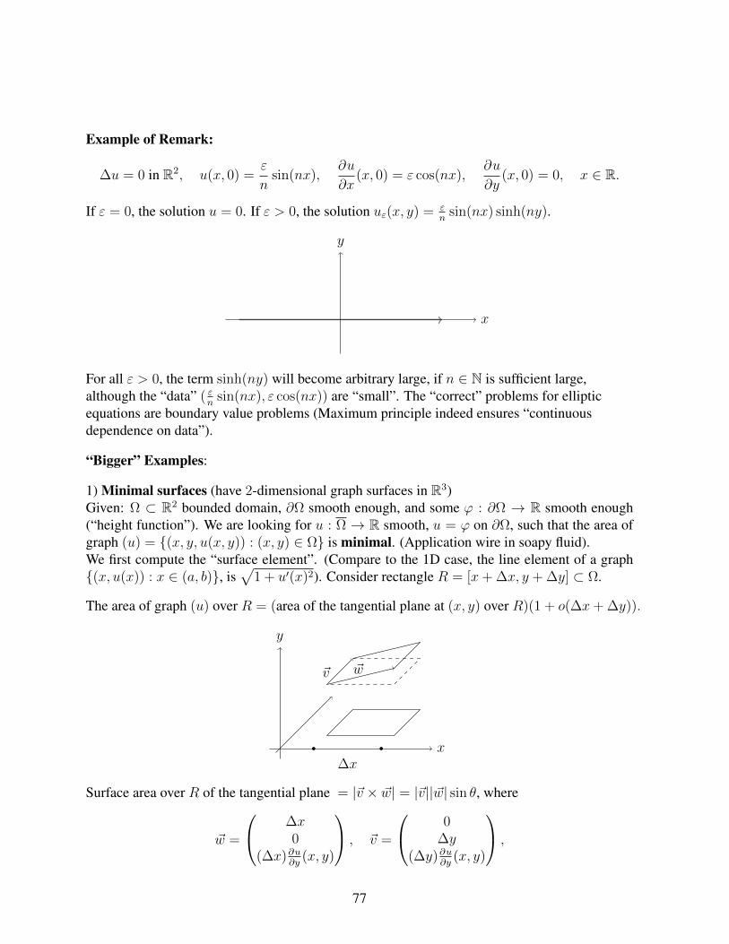
Example of Remark:
∆u = 0 in R2, u(x, 0) =ε
nsin(nx),
∂u
∂x(x, 0) = ε cos(nx),
∂u
∂y(x, 0) = 0, x ∈ R.
If ε = 0, the solution u = 0. If ε > 0, the solution uε(x, y) = εn
sin(nx) sinh(ny).
x
y
For all ε > 0, the term sinh(ny) will become arbitrary large, if n ∈ N is sufficient large,although the “data” ( ε
nsin(nx), ε cos(nx)) are “small”. The “correct” problems for elliptic
equations are boundary value problems (Maximum principle indeed ensures “continuousdependence on data”).
“Bigger” Examples:
1) Minimal surfaces (have 2-dimensional graph surfaces in R3)Given: Ω ⊂ R2 bounded domain, ∂Ω smooth enough, and some ϕ : ∂Ω → R smooth enough(“height function”). We are looking for u : Ω → R smooth, u = ϕ on ∂Ω, such that the area ofgraph (u) = (x, y, u(x, y)) : (x, y) ∈ Ω is minimal. (Application wire in soapy fluid).We first compute the “surface element”. (Compare to the 1D case, the line element of a graph(x, u(x)) : x ∈ (a, b), is
√1 + u′(x)2). Consider rectangle R = [x+ ∆x, y + ∆y] ⊂ Ω.
The area of graph (u) over R = (area of the tangential plane at (x, y) over R)(1 + o(∆x+ ∆y)).
~v ~w
∆xx
y
Surface area over R of the tangential plane = |~v × ~w| = |~v||~w| sin θ, where
~w =
∆x0
(∆x)∂u∂y
(x, y)
, ~v =
0∆y
(∆y)∂u∂y
(x, y)
,
77

so
|~w| = ∆x
√1 +
(∂u
∂x
)2
, |~v| = ∆y
√1 +
(∂u
∂y
)2
, ~v · ~w = (∆x)(∆y)∂u
∂x
∂u
∂y.
So
|~v||~w| sin θ = |~v||~w| ·√
1− cos2 θ = |~v||~w|
√1− ~v · ~w|~v||~w|
=√|~v|2|~w|2 − (~v · ~w)2
= (∆x)(∆y)
√√√√[1 +
(∂u
∂x
)2][
1 +
(∂u
∂y
)2]−(∂u
∂x
)2(∂u
∂y
)2
=
√1 +
(∂u
∂x
)2
+
(∂u
∂y
)2
(∆x)(∆y) =√
1 + |∇u|2(∆x)(∆y).
Then, the surface element is√
1 + |∇u|2dxdy. Hence, the surface of graph (u) is∫Ω
√1 + |∇u|2dxdy.
So the task reads: Minimize
J [u] :=
∫Ω
√1 + |∇u|2dxdy
under the side condition u = ϕ on ∂Ω, which is typical variational problems, and the relatedanalysis is called variational calculus. Let u be a minimizer of this variational problem (exis-tence is non-trivial and will not be addressed here), u sufficiently smooth. For all ψ ∈ C1(Ω)such that ψ = 0 on ∂Ω, and for all λ ∈ R, we have
J [u]︸︷︷︸=:g(0)
≤ J [u+ λψ]︸ ︷︷ ︸=:g(λ)
(note u+ λψ = ϕ on ∂Ω).Thus, g attains its minimal at λ = 0, and hence g′(0) = 0, if g is differentiable.
Indeed,
g(λ)− g(0)
λ=
1
λ
∫Ω
[√1 + |∇(u+ λψ)|2 −
√1 + |∇u|2
]dxdy
=1
λ
∫Ω
2λ∇u · ∇ψ + λ2|∇ψ|2√1 + |∇(u+ λψ)|2 +
√1 + |∇u|2
dxdy
=
∫Ω
2∇u · ∇ψ + λ|∇ψ|2√1 + |∇(u+ λψ)|2 +
√1 + |∇u|2
dxdy.
78

The integral is bounded by∫
Ω2|∇u·∇ψ|+|∇ψ|2
2dxdy with |λ| ≤ 1 and converges pointwise (for a.e.
x ∈ Ω) to∫
Ω∇u·∇ψ√1+|∇u|2
dxdy as λ → 0. So by lebesgue dominated convergence Theorem, g is
differentiable at 0 and
g′(0) =
∫Ω
∇u · ∇ψ√1 + |∇u|2
dxdy.
So our necessary condition reads:∫Ω
∇u · ∇ψ√1 + |∇u|2
dxdy = 0
for all ψ ∈ C1(Ω) such that ψ = 0 on ∂Ω, plus the condition u = ϕ on ∂Ω.Weak formulation of a boundary value problem, which is the so called Euler equation for thegiven variational problem. Assuming now u ∈ C2(Ω), then
0 =
∫Ω
∇u · ∇ψ√1 + |∇u|2︸ ︷︷ ︸
= ∇u√1+|∇u|2
·∇ψ
dxdyGreen′sformula
=
∫∂Ω
∂u∂ν√
1 + |∇u|2ψ︸︷︷︸=0
dσ −∫
Ω
div
(∇u√
1 + |∇u|2
)ψdxdy
all ψ ∈ C1(Ω) (which is dense in L2(Ω)) such that ψ = 0 on ∂Ω. This implies
div
(∇u√
1 + |∇u|2
)= 0
on Ω, and u = ϕ on ∂Ω, which is called the minimal surface equation. This is the strongformulation of the Euler equation for the given variational problem.What is the type of this equation?
div
(∇u√
1 + |∇u|2
)=
∂
∂x
∂u∂x√
1 +(∂u∂x
)2+(∂u∂y
)2
+∂
∂y
∂u∂y√
1 +(∂u∂x
)2+(∂u∂y
)2
=∂2u∂x2√
1 +(∂u∂x
)2+(∂u∂y
)2−
∂u∂x
(∂u∂x
∂2u∂x2 + ∂u
∂y∂2u∂x∂y
)(√
1 +(∂u∂x
)2+(∂u∂y
)2)3 +
∂2u∂y2√
1 +(∂u∂x
)2+(∂u∂y
)2
−∂u∂y
(∂u∂x
∂2u∂x∂y
+ ∂u∂y
∂2u∂y2
)(√
1 +(∂u∂x
)2+(∂u∂y
)2)3 =
1(√1 +
(∂u∂x
)2+(∂u∂y
)2)3 .
79

[(∂2u
∂x2+∂2u
∂y2
)(1 +
(∂u
∂x
)2
+
(∂u
∂y
)2)− ∂2u
∂x2
(∂u
∂x
)2
− ∂2u
∂y2
(∂u
∂y
)2
︸ ︷︷ ︸(1+( ∂u∂y )
2)∂2u∂x2 +
(1+( ∂u∂x )
2)∂2u∂y2
−2∂u
∂x
∂u
∂y
∂2u
∂x∂y
].
Thus
div
(∇u√
1 + |∇u|2
)= 0,
which is equivalent to:(1 +
(∂u
∂y
)2)
︸ ︷︷ ︸=:a
∂2u
∂x2− 2
∂u
∂x
∂u
∂y︸ ︷︷ ︸=:−b
∂2u
∂x∂y+
(1 +
(∂u
∂x
)2)
︸ ︷︷ ︸=:c
∂2u
∂y2= 0︸︷︷︸
=:d
.
Hence, the minimal surface equation is a quasilinear second order differential equation.Moreover,
b2 − ac =
(∂u
∂x
∂u
∂y
)2
−
(1 +
(∂u
∂y
)2)(
1 +
(∂u
∂x
)2)
= −
(1 +
(∂u
∂x
)2
+
(∂u
∂y
)2)< 0,
so, the minimal surface equation is elliptic, with respect to any u.
2) Gas dynamicsCrucial quantities characterizing gas/fluid: mass density ρ = ρ(x, y, z, t), velocity field v =
(x, y, z, t), pressure p = p(x, y, z, t) with functions ρ, p : R3 × [0,∞)→ R, v : R3 × [0,∞)→R3, which we assume to be sufficiently smooth. Here, we neglect internal friction between thefluid molecules.Euler’s equation of motion (Newton’s Law):
ρdv
dt= − grad p+ f
(− grad p is the internal force driving the gas/fluid from high pressure regions to low pressureregions), where the “total” time derivative d
dthas to be understood in “co-moving coordinates”,
i.e. let (x(t), y(t), z(t)) is the trajectory of a particle, then:
dv
dt:=
d
dtv(x(t), y(t), z(t), t) =
∂v
∂x(x(t), y(t), z(t), t)x(t) +
∂v
∂y(x(t), y(t), z(t), t)y(t)
+∂v
∂z(x(t), y(t), z(t), t)z(t) +
∂v
∂t(x(t), y(t), z(t), t);
80

thus, since xyz
(t) = v(x(t), y(t), z(t), t),
dv
dt=
(∂v
∂xv1 +
∂v
∂yv2 +
∂v
∂zv3 +
∂v
∂t
)(x(t), y(t), z(t), t)
=[
(v · ∇)︸ ︷︷ ︸formal writing of
∑3i=1 vi
∂∂xi
v](x(t), y(t), z(t), t) +
∂v
∂t(x(t), y(t), z(t), t).
The term (v · ∇) v is called convection term. Furthermore,
dφ
dt=∂φ
∂t+ (v · ∇)φ ,
for any physical quantity φ. Inserting into Euler’s equation:
ρ
(∂v
∂t+ (v · ∇) v
)+ grad p = f
This is Euler’s equation of fluid dynamics (without friction).With friction, the equation reads
ρ
(∂v
∂t+ (v · ∇) v
)− η∆v + grad p = f,
where η is the viscosity of the gas/fluid and η ∼ 1Re , Re = Reynolds number of the fluid/gas.
The latter equation (with η∆v) is called the Navier-Stokes equation. There are 5 equationsfor the 5 unknown functions (p, ρ, v1, v2, v3).
Moreover, in any fluid/gas we have mass conservation, i.e. the continuity equation holds:
∂ρ
∂t+ div(ρv) = 0
Proof. Let Ω ⊂ R3 be some fixed, bounded domain with smooth boundary to allow the applica-tion of the Gauss Theorem. Let
M(t) :=
∫Ω
ρ(x, y, z, t) d(x, y, z)
be the total mass in Ω at time t. Then
M ′(t)Ω bounded, ρ smooth
=
∫Ω
∂ρ
∂t(x, y, z, t)d(x, y, z).
81
On the other hand,
M ′(t) = −∫∂Ω
ρv︸︷︷︸mass flow
·νdσ Gauss Theorem= −
∫Ω
div(ρv)d(x, y, z).
Hence ∫Ω
[∂ρ
∂t+ div(ρv)
]d(x, y, z) = 0.
Since Ω is arbitrary, this implies
∂ρ
∂t+ div(ρv) = 0.
The incompressible fluids (no gas) satisfy
dρ
dt=∂ρ
∂t+ (v · ∇)ρ = 0.
Comparing with the mass conservation law
∂ρ
∂t+ div(ρv) =
dρ
dt+ ρ div v = 0,
we derive the incompressibility condition:
div v = 0.
If we simply model ρ ≡ constant, the continuity equation also reads div v = 0.For gases, we must work with
∂ρ
∂t+ div(ρv) = 0.
This equation adds to the Euler equation: ρ remains as an unknown function. We need one moreequation (for the 5 unknown, v = (v1, v2, v3), ρ, p) which in gas dynamics is usually a materiallaw, that is, for example, pressure-density law. In the isothermic case (temperature T is constant)we have
ρ = ρ(p) or p = p(ρ),
where ρ : R→ R is a given invertible and smooth function, characterizing the specific gas underconsideration, and p = ρ−1.
82

Example: Ideal gas, characterized by the equation
pV = NRT (R : universal constant),
i.e. p = ρRT , so here,
p(ρ) = ρ RT︸︷︷︸constant in the isothermic case
, ρ(p) =1
RTp,
i.e., linear functions ρ, p.We define
c :=1√ρ′(p)
which is the local speed of sound (depending on p, or ρ, respectively). Then
grad p = c2 grad ρ,
and thus, Euler’s equation becomes
∂v
∂t+ (v · ∇) v +
c2
ρgrad ρ =
1
ρf.
In the stationary case, it reads:
(v · ∇) v +c2
ρgrad ρ =
1
ρf.
The (stationary) continuity equation div(ρv) = 0 adds to this. There are 4 equations for 4unknown functions.
Further assumptions:
1. The flow is vortex-free (irrotational): rot v = 0;
2. The flow is stationary: ∂ρ∂t
= 0, ∂v∂t
= 0;
3. f = 0.
If the spacial domain is simply connected, rot v = 0 implies the existence of a velocity potentialφ such that v = gradφ . Then
[(v · ∇)v]i =∑j
vj∂vi∂xj
=∑j
∂φ
∂xj
∂2φ
∂xj∂xi,
83
so by Euler’s equation
1
ρ
∂p
∂xi= −
∑j
∂φ
∂xj
∂2φ
∂xi∂xj= −1
2
∂
∂xi
(∑j
(∂φ
∂xj
)2). (18)
Thus,
(v · ∇)v +c2
ρgrad ρ = 0
implies
v · grad ρ = − ρc2
[(v · ∇)v] · v = − ρc2
∑i,j
∂φ
∂xi
∂φ
∂xj
∂2φ
∂xi∂xj. (19)
Moreover, by continuity equation,
0 = div(ρv) = (grad ρ) · v + ρ div v︸︷︷︸=gradφ︸ ︷︷ ︸
=∆φ
= ρ∆φ− ρ
c2
∑i,j
∂φ
∂xi
∂φ
∂xj
∂2φ
∂xj∂xi.
Hence, equation of φ reads
c2∆φ =∑i,j
∂φ
∂xi
∂φ
∂xj
∂2φ
∂xi∂xj,
which is called the stream function formulation of the gas problem.Further assumptions: plane flow, i.e. φ is independent of x3. Write again x, y instead of
x1, x2. Then the equation for φ reads[c2 −
(∂φ
∂x
)2
︸ ︷︷ ︸= a
]∂2φ
∂x2− 2
∂φ
∂x
∂φ
∂y︸ ︷︷ ︸= −b
∂2φ
∂x∂y+
[c2 −
(∂φ
∂y
)2
︸ ︷︷ ︸=c
]∂2φ
∂y2= 0.
Type of this equation:
ac− b2 =
[c2 −
(∂φ
∂x
)2 ][c2 −
(∂φ
∂y
)2 ]−(∂φ
∂x
∂φ
∂y
)2
= c4 − c2
[(∂φ
∂x
)2
+
(∂φ
∂y
)2 ]
= c2
[c2 −
[(∂φ
∂x
)2
+
(∂φ
∂y
)2
︸ ︷︷ ︸= | gradφ|2= |v|2
]]= c2(c2 − |v2|)
=
> 0, for |v|< c : subsonic flow, then the problem is elliptic.
< 0, for |v|> c : supersonic flow then the problem is hyperbolic.
84

In supersonic flow problem (example: wings of a fast airplane), there is typically some do-mains |v| < c ( elliptic) and some other domains where |v| > c ( hyperbolic).
Recall in the fluid equation c = 1√ρ′(p)
is not a constant. Let c = c(p). Moreover,
1
ρgrad p = −1
2grad
(|v|2),
implies the surface |v| = constant = p = ˜constant.
85

6 Normal forms for semilinear PDE’s of second order in R2
We consider
a(x, y)∂2u
∂x2+ 2b(x, y)
∂2u
∂x∂y+ c(x, y)
∂2u
∂y2= d
(x, y, u,
∂u
∂x,∂u
∂y
).
Introduce new coordinates
ξ = ϕ(x, y), η = ψ(x, y).
We require
det
(∂ϕ∂x
∂ϕ∂y
∂ψ∂x
∂ψ∂y
)6= 0
everywhere, then the local inversion (x, y) = F (ξ, η) exists. So for u(ξ, η) = u(x, y), i.e.u(x, y) = u(ϕ(x, y), ψ(x, y)), we obtain
∂u
∂x=∂u
∂ξ
∂ϕ
∂x+∂u
∂η
∂ψ
∂x,
∂u
∂y=∂u
∂ξ
∂ϕ
∂y+∂u
∂η
∂ψ
∂y,
∂2u
∂x2=∂2u
∂ξ2
(∂ϕ
∂x
)2
+ 2∂2u
∂ξ∂η
∂ϕ
∂x
∂ψ
∂x+∂2u
∂η2
(∂ψ
∂x
)2
+∂u
∂ξ
∂2ϕ
∂x2+∂u
∂η
∂2ψ
∂x2,
∂2u
∂x∂y=∂2u
∂ξ2
∂ϕ
∂x
∂ϕ
∂y+
∂2u
∂ξ∂η
(∂ϕ
∂x
∂ψ
∂y+∂ϕ
∂y
∂ψ
∂x
)+∂2u
∂η2
∂ψ
∂x
∂ψ
∂y+∂u
∂ξ
∂2ϕ
∂x∂y+∂u
∂η
∂2ψ
∂x∂y,
∂2u
∂y2=∂2u
∂ξ2
(∂ϕ
∂y
)2
+ 2∂2u
∂ξ∂η
∂ϕ
∂y
∂ψ
∂y+∂2u
∂η2
(∂ψ
∂y
)2
+∂u
∂ξ
∂2ϕ
∂y2+∂u
∂η
∂2ψ
∂y2.
From now on, we identify u and u. We insert the results in our original partial differentialequation:
∂2u
∂ξ2
[a
(∂ϕ
∂x
)2
+ 2b∂ϕ
∂x
∂ϕ
∂y+ c
(∂ϕ
∂y
)2
︸ ︷︷ ︸=:A(ξ,η)
]+ 2
∂2u
∂ξ∂η
[a∂ϕ
∂x
∂ψ
∂x+ b
(∂ϕ
∂x
∂ψ
∂y+∂ϕ
∂y
∂ψ
∂x
)+ c
∂ϕ
∂y
∂ψ
∂y︸ ︷︷ ︸=:B(ξ,η)
]
+∂2u
∂η2
[a
(∂ψ
∂x
)2
+ 2b∂ψ
∂x
∂ψ
∂y+ c
(∂ψ
∂y
)2
︸ ︷︷ ︸=:C(ξ,η)
]= d
(x, y︸︷︷︸
=F (ξ,η)
, u,∂u
∂ξ
∂ϕ
∂x+∂u
∂η
∂ψ
∂x,∂u
∂ξ
∂ϕ
∂y+∂u
∂η
∂ψ
∂y
)
−(a∂2ϕ
∂x2+ 2b
∂2ϕ
∂x∂y+ c
∂2ϕ
∂y2
)∂u
∂ξ−(a∂2ψ
∂x2+ 2b
∂2ψ
∂x∂y+ c
∂2ψ
∂y2
)∂u
∂η=: d
(ξ, η, u,
∂u
∂ξ,∂u
∂η
).
86
Goal: Choose ϕ and ψ such that A,B,C become a “simple” standard form. For this, we have todistinguish the type of the original equation.Observation: If the original equation is linear (or linear with respect to ∂u
∂x, ∂u∂y
only), then thesame is true for the new equation.
1. hyperbolic case (ac− b2 < 0 on Ω).We choose ϕ, ψ such that the family of curves on which ϕ is constant or ψ is constant re-spectively, coincide with the two families of characteristic curves. Thus, for characteristiccurves (x1(t), y1(t)) in one family, we want d
dtϕ(x1(t), y1(t)) = 0, and for characteristic
curves (x2(t), y2(t)) in the other family, we want ddtψ(x2(t), y2(t)) = 0. So we want
∂ϕ
∂x(x1(t), y1(t))x1(t) +
∂ϕ
∂y(x1(t), y1(t))y1(t) = 0,
∂ψ
∂x(x2(t), y2(t))x2(t) +
∂ψ
∂y(x2(t), y2(t))y2(t) = 0.
Hence, we obtain (x1
y1
)⊥
(∂ϕ∂x
∂ϕ∂y
),
(x2
y2
)⊥
(∂ψ∂x
∂ψ∂y
),
i.e. (x1
y1
)= λ
(∂ϕ∂y
−∂ϕ∂x
),
(x2
y2
)= µ
(∂ψ∂y
−∂ψ∂x
),
where λ, µ 6= 0 (λ = λ(x, y), µ = µ(x, y)).
Thus, we obtain
det
(∂ϕ∂x
∂ϕ∂y
∂ψ∂x
∂ψ∂x
)= − 1
λµdet
(x1 x2
y1 y2
)6= 0,
since(x1
y1
)and
(x2
y2
)are linearly independent.
Recall that the ODE for the both families of characteristic curves reads
a(x, y)y2 − 2b(x, y)xy + c(x, y)x2 = 0.
Therefore,
0 = λ2
[a(x, y)
(∂ϕ
∂x
)2
+ 2b(x, y)∂ϕ
∂x
∂ϕ
∂y+ c(x, y)
(∂ϕ
∂y
)2]
= λ2A2 ⇒ A ≡ 0,
0 = µ2
[a(x, y)
(∂ψ
∂x
)2
+ 2b(x, y)∂ψ
∂x
∂ψ
∂y+ c(x, y)
(∂ψ
∂y
)2]
= µ2C2 ⇒ C ≡ 0.
87

Moreover,
B(ξ, η) = a∂ϕ
∂x
∂ψ
∂x+ b
(∂ϕ
∂x
∂ψ
∂y+∂ϕ
∂y
∂ψ
∂x
)+ c
∂ϕ
∂y
∂ψ
∂y
=1
λµ[ay1y2 + b(−x2y1 − x1y2) + cx1x2] =
1
λµ
(cx1 − by1
ay1 − bx1
)·(x2
y2
).
Furthermore, by the ODE for(x1
x2
)1
λµ
(cx1 − by1
ay1 − bx1
)·(x1
y1
)=
1
λµ[c(x1)2 − 2bx1y1 + a(y1)2] = 0.
So if B(ξ, η) = 0, we conclude (since(x1
y1
)and
(x2
y2
)are linearly independent)(
cx1 − by1
ay1 − bx1
)=
(00
),
which is contradiction since det
(c −b−b a
)= ac− b2 < 0 and
(x1
y1
)6=(
00
).
So we have B 6= 0 (and A ≡ C ≡ 0). Hence, after dividing by 2B(ξ, η), we get
∂2u
∂ξ∂η= D
(ξ, η, u,
∂u
∂ξ,∂u
∂η
)where D = d
2B. This is the normal form in the hyperbolic case (differential equation in
characteristic coordinates).As seen in Chapter II, the subsequent coordinate transformation x = ξ + η, y = ξ − η,leads to
∂2u
∂x2− ∂2u
∂y2= ˜D
(x, y, u,
∂u
∂x,∂u
∂y
),
which is “wave equation form”, can also be regarded as a normal form.
2+3. elliptic and parabolic case.Assume that the coefficients a, b, c are C1-smooth. Try first to obtain B ≡ 0:
B =
(∂ϕ
∂x,∂ϕ
∂y
)(a bb c
)(∂ψ∂x
∂ψ∂y
)!
= 0,
i.e. (a∂ϕ∂x
+ b∂ϕ∂y
b∂ϕ∂x
+ c∂ϕ∂y
)·
(∂ψ∂x
∂ψ∂y
)!
= 0.
88

Hence, B ≡ 0 if and only if (∂ψ∂x
∂ψ∂y
)= λ
−(b∂ϕ∂x + c∂ϕ∂y
)a∂ϕ∂x
+ b∂ϕ∂y,
(20)
for some λ : Ω→ R.
In order to have a solution ψ for (20), the integrability condition
∂
∂x
[λ
(a∂ϕ
∂x+ b
∂ϕ
∂y
)]+
∂
∂y
[λ
(b∂ϕ
∂x+ c
∂ϕ
∂y
)]= 0 (21)
must be satisfied. This is a second order PDE, with ϕ and λ as unknowns. If λ and ϕ solveit, we can compare ψ from (20). If (20), (21) are satisfied, we obtain
C(ξ, η) = a
(∂ψ
∂x
)2
+ 2b∂ψ
∂x
∂ϕ
∂y+ c
(∂ψ
∂y
)2
(20)= λ2
[a
(b∂ϕ
∂x+ c
∂ϕ
∂y
)2
− 2b
(b∂ϕ
∂x+ c
∂ϕ
∂y
)(a∂ϕ
∂x+ b
∂ϕ
∂y
)+ c
(a∂ϕ
∂x+ b
∂ϕ
∂y
)2]
= λ2
[(ab2 − 2b2a+ ca2︸ ︷︷ ︸
=a(ac−b2)
)(∂ϕ∂x
)2
+(
2abc− 2b3 − 2bca+ 2cab︸ ︷︷ ︸=2b(ac−b2)
)∂ϕ∂x
∂ϕ
∂y
+(ac2 − 2b2c+ cb2︸ ︷︷ ︸
=c(ac−b2)
)(∂ϕ∂y
)2 ]= λ2(ac− b2)A(ξ, η). (22)
In order to obtain a regular coordinate transformation, we must have
0 6= det
(∂ϕ∂x
∂ϕ∂y
∂ϕ∂x
∂ϕ∂y
)=∂ϕ
∂x
∂ϕ
∂y− ∂ϕ
∂y
∂ϕ
∂x
(20)=
∂ϕ
∂x
[λ
(a∂ϕ
∂x+ b
∂ϕ
∂y
)]+∂ϕ
∂y
[λ
(b∂ϕ
∂x+ c
∂ϕ
∂y
)]= λA, (23)
so we must have A 6= 0, λ 6= 0.
2. Elliptic case (ac− b2 > 0 on Ω).We try to get A = C. By (22), we have to choose
λ :=1√
ac− b26= 0.
89

Moreover, to satisfy (23)
A =
(∂ϕ
∂x,∂ϕ
∂y
)(a bb c
)(∂ϕ∂x
∂ϕ∂y
)6= 0,
so we need(∂ϕ∂x∂ϕ∂y
)6=(
00
)in Ω.
Rewriting (21) with the above choice for λ,
∂
∂x
[a∂ϕ∂x
+ b∂ϕ∂y√
ac− b2
]+
∂
∂y
[b∂ϕ∂x
+ c∂ϕ∂y√
ac− b2
]= 0,
which is a linear second order equation for ϕ. This is the Beltrami equation. It has to besolved under the side condition
(∂ϕ∂x, ∂ϕ∂y
)6= (0, 0) everywhere.
Divide the equation for u by A(= C), we get with D = dA
:
∂2u
∂ξ2+∂2u
∂η2= D
(ξ, η, u,
∂u
∂ξ,∂u
∂η
),
which is the normal form in the elliptic case (nonlinear Poisson equation).
3. Parabolic case (ac− b2 = 0 on Ω).Additional assumption (to avoid a totally degenerate equation): For every (x, y) ∈ Ω, atleast one of the three values: a(x, y), b(x, y), c(x, y), is no zero.Hence, we have a 6= 0 or c 6= 0 everywhere. Locally we can assume a 6= 0 at some givenpoint. Without loss of generality, let a > 0. Then c = b2
a≥ 0.
The eigenvalues of(a bb c
)are (note ac = b2):
0
(eigenvector
(−ba
))and a+ c
(eigenvector
(ab
)).
We had already achieved B ≡ 0 ((20), (21)). Moreover, by (22)
C ≡ λ2(ac− b2︸ ︷︷ ︸=0
)A = 0.
We are left to satisfy (23) and to discuss (21). We can write(∂ϕ∂x
∂ϕ∂y
)= µ1
(ab
)+ µ2
(−ba
), (24)
with coefficient functions µ1, µ2 : Ω→ R.
90
Integrability condition:
∂
∂y(µ1a− µ2b) =
∂
∂x(µ1b− µ2a), (25)
which is a PDE for µ1 and µ2. Then, ϕ can be computed from (24). Then,
A =
(∂ϕ
∂x,∂ϕ
∂y
)(a bb c
)(∂ϕ∂x
∂ϕ∂y
)=
(∂ϕ
∂x,∂ϕ
∂y︸ ︷︷ ︸=µ1(a,b)+µ2(−b,a)
)(a bb c
)[µ1
(ab
)+ µ2
(−ba
)]︸ ︷︷ ︸
=µ1(a+c)
ab
= µ2
1(a+ c︸ ︷︷ ︸>0
)(a2 + b2︸ ︷︷ ︸>0
).
Then, A 6= 0, if and only if µ1 6= 0. This is a side condition for (25). The equation (21)now reads
∂
∂x[λµ1(a+ c)a] +
∂
∂y[λµ1(a+ c)b] = 0,
since, (a bb c
)(∂ϕ∂x
∂ϕ∂y
)= µ1(a+ c)
(ab
).
Putting λ = λµ1(a+ c), this equation becomes
∂
∂x(λa) +
∂
∂y(λb) = 0, (26)
with the side condition λ 6= 0.
Hence, determine µ1 and µ2 from (25), under the side condition µ1 6= 0, then λ (from (26)),under the side condition λ 6= 0, then λ := λ
µ1(a+c), then ϕ from (24) and finally ψ from (20).
Defining D = dA
, we get the normal form of the original equation in the new coordinate
∂2u
∂ξ2= D
(ξ, η, u,
∂u
∂ξ,∂u
∂η
),
which is the normal form in the parabolic case.If the original equation is linear in ∂u
∂x, ∂u∂y
, then also the transformed equation is linear in ∂u∂ξ
and ∂u∂η
(see earlier observation). So the normal form achieved so far reads
∂2u
∂ξ2= α(ξ, η)
∂u
∂ξ+ β(ξ, η)
∂u
∂η+ γ(ξ, η, u).
91

Assume now that β 6= 0 locally. (Note: If β ≡ 0, the equation is an ODE).Transform ξ = χ(ξ, η), η = η, where
χ(ξ, η) :=
∫ ξ√|β(t, η)|dt.
Then
det
(∂ ξ∂ξ
∂ ξ∂η
∂ η∂ξ
∂ η∂η
)= det
(√|β(ξ, η)| ?
0 1
)=√|β(ξ, η)| 6= 0.
We find
∂u
∂ξ=∂u
∂ξ
∂ξ
∂ξ+∂u
∂η
∂η
∂ξ︸︷︷︸=0
=√|β(ξ, η)|∂u
∂ξ,
∂u
∂η=∂u
∂ξ
∂ξ
∂η+∂u
∂η
∂η
∂η︸︷︷︸=1
=
[∫ ξ ∂β∂η
(t, η)√|β(t, η)|
2β(t, η)dt
]∂u
∂ξ+∂u
∂η.
So
∂2u
∂ξ2= |β(ξ, η)|∂
2u
∂ξ2+
∂β∂ξ
(ξ, η)√|β(ξ, η)|
2β(ξ, η)
∂u
∂ξ.
Insert everything into differential equation
|β(ξ, η)|∂2u
∂ξ2+
∂β∂ξ
√|β(ξ, η)|
2β(ξ, η)
∂u
∂ξ= α(ξ, η)
√|β(ξ, η)|∂u
∂ξ
+ β(ξ, η)
[∫ ξ ∂β∂η
(t, η)√|β(t, η)|
2β(t, η)dt
]∂u
∂ξ+∂u
∂η
+ γ(ξ, η, u(ξ, η))︸ ︷︷ ︸
=γ(ξ,η,u)
.
Diving by |β(ξ, η)|:
∂2u
∂ξ2=
1√|β(ξ, η)|
[α(ξ, η)−
∂β∂ξ
2β(ξ, η)
]∂u
∂ξ+
β(ξ, η)
|β(ξ, η)|
[∫ ξ ∂β∂η
(t, η)√|β(t, η)|
2β(t, η)dt
]∂u
∂ξ︸ ︷︷ ︸=α(ξ,η) ∂u
∂ξ
+β(ξ, η)
|β(ξ, η)|︸ ︷︷ ︸=σ∈1,−1
∂u
∂η+γ(ξ, η, u)
|β(ξ, η)|︸ ︷︷ ︸=˜γ(ξ,η,u)
.
92

If σ = −1, transform ˜ξ = ξ, ˜η = −η, which gives:
∂2u
∂ ˜ξ=∂u
∂ ˜η+ a( ˜ξ, ˜η)
∂u
∂ ˜ξ+ ˜γ( ˜ξ, ˜η, u).
Last step: Use one more transformation to make a vanish. (exercise).
93

7 An existence and uniqueness result for the semilinear hy-perbolic initial value problem
We consider
a(x, y)∂2u
∂x2+ 2b(x, y)
∂2u
∂x∂y+ c(x, y)
∂2u
∂y2= d
(x, y, u,
∂u
∂x,∂u
∂y
),
where now b2 − ac > 0 everywhere (hyperbolic case). Compute characteristics and transforminto normal form (have rename the new coordinates ξ and η as x and y, and the new right-handside as d again):
∂2u
∂x∂y= d
(x, y, u,
∂u
∂x,∂u
∂y
).
Assume that d is continuous. Suppose that initial conditions are given on a new coordinatearea in R2. Recall that the characteristics in this normal form are given by x = constant andy = constant. So a curve (x(t), y(t)) is non-characteristic iff x(t) 6= 0 and y(t) 6= 0. Then thecurve can also be assumed to be given in the form y = g(x) or x = h(y), where g, h ∈ C1,g′ 6= 0, h′ 6= 0 and h = g−1.
The initial conditions on this curve are written as
u(x, g(x)) = ϕ(x),∂u
∂x(x, g(x)) = ψ1(x),
∂u
∂y(x, g(x)) = ψ2(x), ∀x ∈ [a, b]
where ϕ ∈ C1[a, b], ψ1(x), ψ2(x) ∈ C[a, b], are given.Let [α, β] = g([a, b]). We look for a solution u on [a, b]× [α, β].Recall the Picard-Lindelof for the ODE’s:
y′ = f(x, y), y(0) = y0.
We write the problem equivalent as an integral equation
y(x) = y0 +
∫ x
0
f(x, y(t))dt =: (Ty)(x), x ∈ [a, b].
We use the Banach’s Pixed-Point-Theorem. We define the Banach space (X, ‖ · ‖) as following
X = C[a, b], ‖y‖ := maxx∈[a,b]
|y(x)|eNx
, N > 0 constant.
Suppose that f satisfies a global Lipschitz condition w.r.t. y, i.e.
|f(x, y)− f(x, y)| ≤ L|y − y|.
94

Then
|(Ty)(x)− (T y)(x)| =∣∣∣∣∫ x
0
[f(x, y(t))− f(x, y(t))]dt
∣∣∣∣ ≤ ∫ x
0
|f(x, y(t))− f(x, y(t))|︸ ︷︷ ︸≤L|y(t)−y(t)|
dt
≤ L
∫ x
0
|y(t)− y(t)|eNx︸ ︷︷ ︸≤‖y−y‖
eNxdt ≤ L
N‖y − y‖(eNx − 1) ≤ L
N‖y − y‖eNx.
Divide by eNx, take
maxx∈[a,b]
‖Ty − T y‖ ≤ L
N‖y − y‖.
Choose N > L, then T is a contraction on (C[a, b], ‖ · ‖). So by Banach’s FPT, there exists aunique fixed-point y of T , i.e. a unique solution to the given initial value problem.Goals for our hyperbolic initial value problem:
1. Rewrite problem as an integral equation,
2. Apply Banach’s FPT in an appropriated Banach space.
(1) We first consider the special equation
∂2u
∂x∂y= r(x, y),
where r ∈ C([a, b]× [α× β]) and plus the given initial condition.
General solution = general homogeneous solution + one special solution
i) Special solution:
∂2us∂x∂y
= r(x, y) ⇒ ∂us∂x
(x, y) =
∫ y
g(x)
r(x, η) dη
⇒ us(x, y) =
∫ x
h(y)
(∫ y
g(ξ)
r(ξ, η)dη
)dξ.
Then
∂us∂y
(x, y) = −h′(y)
∫ y
g(h(y))︸ ︷︷ ︸=y
r(h(y), η)dη +
∫ x
h(y)
r(ξ, y)dξ =
∫ x
h(y)
r(ξ, y)dξ.
So we have us(x, g(x)) = ∂us∂x
(x, g(x)) = ∂us∂y
(x, g(x)) = 0, x ∈ [a, b].
95
ii) General homogeneous solution: ∂uh∂x∂y
= 0 has general solutions
uh(x, y) = w1(x) + w2(y)
with arbitrary C1-functions w1, w2. We need uh satisfy the initial conditions:
uh(x, g(x)) = ϕ(x) requires w1(x) + w2(g(x)) = ϕ(x) (x ∈ [a, b]),
∂uh∂x
(x, g(x)) = ψ1(x) requires w′1(x) = ψ1(x) (x ∈ [a, b]), i.e.
w1(x) =
∫ x
ψ1(t)dt
∂uh∂y
(x, g(x)) = ψ2(x) requires w′2(g(x)) = ψ2(x) (x ∈ [a, b])︸ ︷︷ ︸( ⇔ w′2(y)=ψ2(h(y)), y∈[α,β])
, i.e.
w2(x) =
∫ y
ψ2(h(s))ds
So
uh(x, y) =
∫ x
ψ1(t)dt+
∫ y
ψ2(h(s))ds.
Derivative in w1(x) + w2(g(x)) = ϕ(x) gives:
ψ1(x) + ψ2 · g′(x) = ϕ′(x)
So the free constant in w1, w2 can be chosen to satisfy w1(x) + w2(x) = ϕ(x).The solution (inhomogeneous) is of the form:
u(x, y) = uh(x, y)︸ ︷︷ ︸depends only on initial condition (by construction)
+us(x, y)︸ ︷︷ ︸depends on r
Rename uh(x, y) = u0(x, y), then
u(x, y) = u0(x, y)︸ ︷︷ ︸independent of r
+
∫ x
h(y)
(∫ y
g(ξ)
r(ξ, η)dη
)dξ
Returning to the original semilinear problem, we immediately see that it is equivalent tothe integral equation
u(x, y) = u0(x, y)︸ ︷︷ ︸fixed
+
∫ x
h(y)
(∫ y
g(ξ)
d
(ξ, η, u(ξ, η),
∂u
∂x(ξ, η),
∂u
∂y(ξ, η)
)dη
)dξ.
96

Moreover, for the above formula
∂u
∂x=∂u0
∂x(x, y) +
∫ y
g(x)
d
(ξ, η, u(ξ, η),
∂u
∂x(ξ, η),
∂u
∂y(ξ, η)
)dη,
∂u
∂y=∂u0
∂y(x, y) +
∫ x
h(y)
d
(ξ, η, u(ξ, η),
∂u
∂x(ξ, η),
∂u
∂y(ξ, η)
)dξ.
We therefore get the following system equation for U =
U1
U2
U3
:=
u∂u∂x∂u∂y
.
U1(x, y) = u0(x, y) +
∫ x
h(y)
(∫ y
g(ξ)
d (ξ, η, U1(ξ, η), U2(ξ, η), U3(ξ, η)) dη
)dξ
=:
TU1
U2
U3
1
(x, y),
U2(x, y) =∂u0
∂x(x, y) +
∫ y
g(x)
d (ξ, η, U1(ξ, η), U2(ξ, η), U3(ξ, η)) dη
=:
TU1
U2
U3
2
(x, y),
U3(x, y) =∂u0
∂y(x, y)
∫ x
h(y)
d (ξ, η, U1(ξ, η), U2(ξ, η), U3(ξ, η)) dξ
=:
TU1
U2
U3
3
(x, y).
This defines an operator T : (C([a, b]× [α× β]))3 → (C([a, b]× [α× β]))3. The orig-inal initial value problem (with u such that u, ∂u
∂x, ∂u∂y, ∂2u∂x∂y
exist and are continuous on[a, b] × [alpha, β]) is equivalent to the integral system for
(U1, U2, U3
)(with U1, U2, U3
continuous).
If u is a solution of the initial value problem with the above smoothness, then
U1
U2
U3
:= u∂u∂x
∂u∂y
is a solution of the integral system (as shown above).
97

2) We have to prove existence and uniqueness for the integral system, using Banach’s Fixed-Pointtheorem. Let
X := C([a, b]× [α, β])3,
TU1
U2
U3
(x, y) =
u0(x, y) +
∫ x
h(y)
(∫ y
g(ξ)
d (ξ, η, U1(ξ, η), U2(ξ, η), U3(ξ, η)) dη
)dξ
∂u0
∂x(x, y) +
∫ y
g(x)
d (ξ, η, U1(ξ, η), U2(ξ, η), U3(ξ, η)) dη
∂u0
∂y(x, y) +
∫ y
h(y)
d (ξ, η, U1(ξ, η), U2(ξ, η), U3(ξ, η)) dξ
.
We define the norm ∥∥∥∥∥∥U1
U2
U3
∥∥∥∥∥∥X
:= max‖U1‖, ‖U2‖, ‖U3‖,
where
‖u‖ := max
|u(x, y)|eN(x+y)
: (x, y) ∈ [a, b]× [α, β]
with N > 0 still arbitrary.
Theorem 7.1. Let d be continuous (as already assumed), and let d satisfies a Lipschitz conditionof the form
|d(x, y, u, p, q)− d(x, y, u, p, q)| ≤ L(|u− u|+ |p− p|+ |q − q|)
for all x ∈ [a, b], y ∈ [α, β] and u, p, q, u, p, q ∈ R, where L > 0 is a fixed constant. The integralsystem (and hence the original initial value problem) has a unique solution on [a, b]× [α, β].
Proof. Here only for the case g′ < 0 on [a, b] (not for the case g′ > 0 on [a, b])Moreover, we prove existence and uniqueness only on Ω+ := (x, y) ∈ [a, b] × [α, β] : y ≥
g(x).(General case: exercises.) We consider X = C(Ω+)3, and∥∥∥∥∥∥U1
U2
U3
∥∥∥∥∥∥X
:= max‖U1‖, ‖U2‖, ‖U3‖,
where k > 0 constant to be chosen later and
‖u‖ := max
|u(x, y)|ek(x+y)
: (x, y) ∈ Ω+
.
98

(X, ‖ · ‖X) is a Banach space. (Following from (C(compact set), ‖ · ‖∞) is a Banach space.)Left to show: T is contractive with respect to ‖ · ‖X , if k is chosen appropriately. So, let’s
calculate ∣∣∣∣∣∣TU1
U2
U3
− TU1
U2
U3
1
∣∣∣∣∣∣≤∫ x
h(y)
(∫ y
g(ξ)
∣∣∣∣d (ξ, η, U1, U2, U3)− d(ξ, η, U1, U2, U3
) ∣∣∣∣︸ ︷︷ ︸≤ L(|U1 − U1|︸ ︷︷ ︸
|U1−U1|ek(ξ+η)
ek(ξ+η)≤ ‖U1−U1‖ek(ξ+η)
+|U2−U2|+|U3−U3|) dη
)dξ
≤ L(‖U1 − U1‖+ ‖U2 − U2‖+ ‖U3 − U3‖
)∫ x
h(y)
(∫ y
g(ξ)
ek(ξ+η)dη
)︸ ︷︷ ︸
= ekξ· 1k
(eky−ekg(ξ))≤ 1k·ek(ξ+y)
dξ
≤ 3L
∥∥∥∥∥∥U1
U2
U3
−U1
U2
U3
∥∥∥∥∥∥X
∫ x
h(y)
1
kek(ξ+y)dξ︸ ︷︷ ︸
= 1k2 [ek(x+y)−ek(h(y)+y)]≤ 1
k2 ek(x+y)
.
Dividing by ek(x+y) and taking the maximum over (x, y) ∈ Ω+ given∥∥∥∥∥∥TU1
U2
U3
− TU1
U2
U3
1
∥∥∥∥∥∥ ≤ 3L
k2
∥∥∥∥∥∥U1
U2
U3
−U1
U2
U3
∥∥∥∥∥∥X
.
Moreover,∣∣∣∣∣∣TU1
U2
U3
− TU1
U2
U3
2
(x, y)
∣∣∣∣∣∣≤∫ y
g(x)
∣∣∣∣d (x, η, U1, U2, U3)− d(x, η, U1, U2, U3
) ∣∣∣∣︸ ︷︷ ︸≤L(|U1−U1|+|U3−U2|+|U3−U3|)≤L(‖U1−U1‖+‖U3−U2‖+‖U3−U3‖)ek(x+η)
dη
≤ 3L
∥∥∥∥∥∥U1
U2
U3
−U1
U2
U3
∥∥∥∥∥∥X
∫ y
g(x)
ek(x+η)dη︸ ︷︷ ︸= 1
k(ek(x+y)−ek(x+g(x)))
≤ 3L
k
∥∥∥∥∥∥U1
U2
U3
−U1
U2
U3
∥∥∥∥∥∥X
ek(x+y).
99
As before, we get now∥∥∥∥∥∥TU1
U2
U3
− TU1
U2
U3
2
∥∥∥∥∥∥ ≤ 3L
k
∥∥∥∥∥∥U1
U2
U3
−U1
U2
U3
∥∥∥∥∥∥x
.
Analogously:∥∥∥∥∥∥TU1
U2
U3
− TU1
U2
U3
∥∥∥∥∥∥X
≤ max
3L
k2,3L
k
︸ ︷︷ ︸
< 1, if we choose k>max3L,1
·
∥∥∥∥∥∥U1
U2
U3
−U1
U2
U3
∥∥∥∥∥∥X
.
So T is contractive on X .
The assumption of global Lipschitz continuity is very strong. (Note that d(x, y, u, p, q) = u2
does not satisfy it.)We can however make the much weaker assumption of a local Lipschitz condition, we’ll
obtain a slightly weaker existence result. For each compact set K ⊂ R3, there exists an L =L(K) such that
|d(x, y, u, p, q)− (x, y, u, p, q)| ≤ L(|u− u|+ |p− p|+ |q − q|)
for all (x, y) ∈ [a, b] × [α, β] and all
upq
,
upq
∈ K. Sufficient for this local Lipschitz
condition is: d, ∂d∂u, ∂d∂p, ∂d∂q
exist and are continuous.
Theorem 7.2. Assumptions as in Theorem 7.1, but with a local instead of global Lipschitz con-dition for d. Then, the initial value problem has a unique solution in [a, b]× [α, β]∩U , where Uof the initial curve.
Proof. Let K = [−γ, γ]3 denote some cube containing (ϕ(x),Ψ1(x),Ψ2(x)) : x ∈ [a, b] in
the interiorK.
We define, for all u ∈ R,
u# =
−γ, if u ≤ −γ,
u, if −γ ≤ u ≤ γ,
γ, if u ≥ γ,
and define
d(x, y, u, p, q) := d(x, y, u#, p#, q#).
100

Easy to show: d satisfies a global Lipschitz condition on [a, b]× [α, β]× R3.Then, by Theorem 7.1, the initial value problem with d instead of d has a unique solution u on[a, b]× [α, β].
Since (u, ∂u∂x, ∂u∂y
) ∈K for (x, y) on the initial curve and are continuous. We find that
(u, ∂u∂x, ∂u∂y
) ∈ K for (x, y) in some neighborhood U of the initial curve.
Hence, d(x, y, u(x, y), ∂u
∂x(x, y), ∂u
∂y(x, y)
)= d
(x, y, u(x, y), ∂u
∂x(x, y), ∂u
∂y(x, y)
)for (x, y) ∈
U . Thus, u solves the given problem with d on U .
101
8 Type classification for semi linear second oeder differentialequations in n variables
First consider the special problem
utt =∂2u
∂t2= F (x, t, u, ux, ut, uxx, uxt)
where t ∈ R, x ∈ Rn, ux =(∂u∂x1, . . . , ∂u
∂xn
), uxx =
(∂2u
∂xi∂xj
)i,j=1,...,n
, uxt =(
∂2u∂x1∂t
, . . . , ∂2u∂xn∂t
)and where F is given and analytic in all its variables. In additional, we consider the initialcondition u(x, 0) = ϕ(x), ut(x, 0) = ψ(x) for x ∈ Rn with analytical functions ϕ, ψ. Note that(x, 0) : x ∈ Rn is a hyperplane in Rn+1. So the initial curve we considered earlier in the caseof two independent variables has now become an initial hyperplane.
From the initial condition u(x, 0) = ϕ(x), x ∈ Rn we obtain ux(x, 0) = ϕx(x), uxx(x, 0) =ϕxx(x), uxxx(x, 0) = ϕxxx(x), . . . (all derivatives with respect to x).From the initial conditionut(x, 0) = ψ(x) (x ∈ Rn) we obtain uxt(x, 0) = ψx(x), uxxt(x, 0) = ψxx(x), uxxxt(x, 0) =ψxxx(x), . . . .
From the differential equation we get
utt(x, 0) = F (x, 0, u(x, 0), ux(x, 0), ut(x, 0), uxx(x, 0), uxt(x, 0)︸ ︷︷ ︸all given in terms of ϕ,ψ
), uttx, uttxx, uttxxx, . . .
all in terms of ϕ, ψ.Differentiating the differential equation gives ∂3u
∂t3in terms of derivatives of which are at most of
order 2 in t. Evaluate this on the initial surface, differentiate with respect to x uttt, utttx, utttxx, . . .all in term of ϕ, ψ.Repeatedly differentiating the differential equation with respect to t, evaluating on the initial sur-face, and differentiating with respect to x, gives all derivatives of u on the initial surface in termsof ϕ, ψ, F and their derivatives.
Theorem 8.1 (Cauchy-Kovalevskaya). Let F, ϕ, ψ be analytic. Then the initial value problemhas an analytic solution on a neighborhood of the initial surface. This solution is unique withinthe class of analytic functions.
Proof. Using the knowledge of all derivatives of any analytic solution on the initial surface (seeabove), the desired solution can be put up by local Taylor series (with expansion points on thesurface). Details are omitted here.
Now consider a more general semilinear differential equation of seconder order:
n∑i,j=1
aij(x)∂u
∂xi∂xj= F (x, u, ux)
Let A(x) := (ai,j(x))i,j=1,...,n. Without loss of generality, let A(x) be symmetric.
102

[ Because
n∑i,j=1
aij(x)∂2u
∂xi∂xj=
1
2
n∑i,j=1
aij(x)∂2u
∂xi∂xj+
n∑i,j=1
aij(x)∂2u
∂xj∂xi︸ ︷︷ ︸= ∂2u
∂xi∂xjif u∈C2
=n∑
i,j=1
1
2(aij(x) + aji(x))
∂2u
∂xi∂xj
i.e. the expressionn∑
i,j=1
aij(x)∂2u
∂xi∂xj
stays the same when A is replaced by 12(A+ AT ).]
Initial conditions:Letϕ : Rn → R be a C2-function, ϕx(x) 6= 0, ∀x ∈ Rn, i.e. ∀x ∈ Rn ∃ i ∈ 1, . . . , n ∂ϕ
∂xi(x) 6=
0. Then, M := x ∈ Rn : ϕ(x) = 0 is a C2-hypersurface in Rn. [Proof: Let x0 ∈ Rn,ϕ(x0) = 0. There exists i ∈ 1, . . . , n such that ∂ϕ
∂xi(x0) 6= 0. Hence, by the Implicit Function
Theorem, the equation ϕ(x) = 0 can locally be solved for xi: xi = f(x1, . . . , xi−1, xi+1, . . . , xn).SoM can locally (in a neighborhood of x0) be written as the graph of the C2 function f .]
Suppose that onM the initial conditions are given
u(x) = g(x), ux(x) = h(x), x ∈M
with g, h are given C2-functions.Compatibility conditions: LocallyM is a graph:
x1 = f(x1, . . . , xi−1, xi+1, . . . , xn)
without loss of generality i = 1 (otherwise rename coordinates), i.e. x1 = f(x2, . . . , xn).So the first initial conditions read
u(f(x2, . . . , xn), x2, . . . , xn) = g(f(x2, . . . , xn), x2, . . . , xn),
ux(f(x2, . . . , xn), x2, . . . , xn) = h(f(x2, . . . , xn), x2, . . . , xn).
Differentiate with respect to xi(i ∈ 2, . . . , n):
∂u
∂xi︸︷︷︸= h1
(f(x2, . . . , xn), x2, . . . , xn)∂f
∂xi(x2, . . . , xn) +
∂u
∂xi︸︷︷︸= hi
(f(x2, . . . , xn), x2, . . . , xn)
=∂g
∂xi(f(x2, . . . , xn), x2, . . . , xn)
∂f
∂xi(x2, . . . , xn) +
∂g
∂xi(f(x2, . . . , xn), x2, . . . , xn).
103

So we get the compatibility condition reads
h1∂f
∂xi+ hi =
∂g
∂xi
∂f
∂xi+∂g
∂xi(i = 2, . . . , n).
Question: Can we solve the differential equation for one second derivative ∂2u∂x2i, such that the
initial hypersurface becomes (locally) the hyperplane xi = 0?To answer this question, we introduce new variables coordinates (locally). In the neighbor-
hood of a given point in M, we can write M as a graph x1 = f(x2, . . . , xn) (without loss ofgenerality we solve x, according to the corresponding condition ∂ϕ
∂x16= 0). Introducing
y =
y1
y2...yn
=
ϕ(x1, . . . , xn)
x2...xn
=: φ(x).
Then the Jacobian of φ is
Jφ(x) =
∂ϕ∂x1
∂ϕ∂x2
· · · ∂ϕ∂xn
0 1 · · · 0...
... . . . ...0 0 · · · 0 1
,
so detJφ(x) = ∂ϕ∂x1
(x) 6= 0 in the neighborhood considered. The hypersurfaceM = x ∈ Rn :ϕ(x) = 0 locally is, in the new coordinates, the hyperplane y1 = 0.
Thus (with the Cauchy-Kovalevskaya situation in view), we have to check if the differentialequation can be written in the form
∂2u
∂y21
= G
(y, n,
∂u
∂y1
, . . . ,∂u
∂yn,∂2u
∂y1∂y2
, . . .︸ ︷︷ ︸all second derivatives except ∂
2u
∂y21
).
For this purpose, we have to write the differential equation in the new coordinates:
∂u
∂xj=
n∑i=1
∂u
∂yi
∂φi∂xj
;∂2u
∂xj∂xk=
n∑i=1
[n∑l=1
∂2u
∂yi∂yl
∂φi∂xj
∂φl∂xl
+∂u
∂yi
∂2φi∂xj∂xk
].
Insert into differential equation:
n∑j,k=1
aj,k∂2u
∂xj∂xk=
n∑i,j,k,l=1
(aj,k
∂φi∂xj
∂φl∂xk
)∂2u
∂yi∂yl+
n∑i,j,k=1
(aj,k
∂2φi∂xj∂xk
)∂u
∂yi= F (x, u, ux).
104

The right hand side can be written in the form F (y, u, uy) (using the local coordinates transfor-mation). So the differential equation in new coordinates reads
n∑i,l=1
ai,l∂2u
∂yi∂yl= F (y, u, uy)−
n∑i=1
bi(y)∂u
∂yi=: ˜F (y, u, uy).
where
ai,l(y) =
(n∑
j,k=1
aj,k∂φi∂xj
∂φl∂xk
) φ−1(y), bi(y) =
(n∑
j,k=1
aj,k∂2u
∂xj∂xk
) φ−1(y).
Hence,
a11(y) =
(n∑
j,k=1
aj,k∂φ1
∂xj
∂φ1
∂xk
) φ−1(y)
=
(n∑
j,k=1
aj,k∂ϕ
∂xj
∂ϕ
∂xk
) φ−1(y) =
(ϕTxAϕx
) φ−1(y).
Thus, the question is: Is ϕTxAϕx 6= 0? If so, we can divide by a11 and get Cauchy-Kovalevskayasituation
∂2u
∂y21
= G
(y, n,
∂u
∂y1
, . . . ,∂u
∂yn,∂2u
∂y1∂y2
, . . .
).
Definition: A vector α ∈ Rnr0 has characteristic direction at ξ ∈M, if αTA(ξ)α = 0. ThehypersurfaceM is called characteristic at ξ ∈ Rn, if ϕx(ξ)TA(ξ)ϕx(ξ) = 0. The hypersurfaceM is called characteristic surface, ifM is characteristic in every ξ ∈M.Also the closure of every characteristic surface is called characteristic surface. M is callednon-characteristic, if there is no point ξ ∈M in which it is characteristic.Remark: Let n = 2. Is the new definition consistent with the old one? The equation reads
a∂2u
∂x21
+ 2b∂2u
∂x1∂x2
+ c∂2u
∂x22
= d
(x1, x2, u,
∂u
∂x1
,∂u
∂x2
).
So the matrix A = (aij)i,j=1,...,n now reads A =
(a bb c
). According to the old definition, the
curve is characteristic at ξ of the tangential vector has characteristic direction. According to thenew definition, the curve is characteristic at ξ of the normal vector has characteristic direction.
But, let an initial curve(x(t)y(t)
)be given (with (x, y) 6= (0, 0) everywhere), as described in
Chapter 5. So we can write locally as y = y(x) or x = x(y). Here we consider only y = ψ(x).
105

We have to writeM = (x, y) : y = ψ(x) (this is our curve) in the form ϕ(x, y) = 0. Thisis true for ϕ(x, y) := y − ψ(x). Hence
(∇ϕ)(x, y) =
(−φ′(x)
1
)and thus
(∇ϕ)TA∇ϕ = (−ψ′(x), 1)
(a bb c
)(−ψ′(x)
1
)= a(ψ′(x))2 − 2bψ′(x) + c.
So we have a coincidence of old and new definition.Examples:
1. Spatially 2D wave equation
∂u
∂t2= ∆u =
∂2u
∂x2+∂2u
∂y2,
which is equivalent to
3∑i,j=1
aij∂2u
∂xi∂xj= 0, where A =
1 0 00 −1 00 0 −1
.
Hence α has characteristic direction if and only if α21 − α2
2 − α23 = 0. If α has charac-
teristic direction, then α1 6= 0, hence without loss of generality α1 = 1. So then α hascharacteristic direction id α2
2 + α23 = 1, i.e.
(α2
α3
)=
(cos θsin θ
)for some θ ∈ [0, 2π), i.e. α =
1cos θsin θ
.
So then α enclose a 45 angle with the (x2, x3)-plane. Hence, characteristic surfaces aresuch hypersurfaces (or closures of these), the normal vector of which everywhere enclo-sures a 45 angle with the (x2, x3)-plane.Examples:
x2
x1
x3
x2
x1
x3
x2
x1
x3
106

2. Poisson equation
∆u =n∑i=1
∂2u
∂x2i
= r(x)
so A = I . Hence, αTAα = |α|2 6= 0 for every α ∈ Rn r 0. So there is no characteristicdirection.
3. Heat equation
∂u
∂t= ∆u =
n∑i=1
∂2u
∂x2i
,
i.e. introducing xn+1 = t:n∑i=1
∂2u
∂x2i
+ 0 · ∂2u
∂x2n+1
=∂u
∂xn+1
,
so
A =
1 0
. . .1
0 0
, and αTAα =n∑i=1
α2i
Hence α ∈ Rn+1 r 0 has characteristic direction if α1, . . . , αn = 0, i.e. α =
0...01
.
So characteristic surfaces are precisely the hypersurfaces xn+1 = constant i.e. t =constant.
Back to the general case. For simplicity, transform A(x), for fixed x, into diagonal form: Thereexists T ∈ Rn×n such that T tAT = diag(λ1, . . . , λn) (T and λ1, . . . , λn depends on x).Then
αTAα = (αTT )(T TAT )(T Tα) = β
λ1
. . .λn
β,
where β = T Tα. β 6= 0⇔ α 6= 0. So
αTAα = 0⇐⇒n∑i=1
λiβ2i = 0.
Definition: The differential equation is called
107
• elliptic at ξ ∈ Rn, if all eigenvalues of A(ξ) have the same sign. (all positive or allnegative.)
• hyperbolic at ξ ∈ Rn, if one eigenvalue of A(ξ) is positive and all others are negative orone eigenvalue of A(ξ) is negative and all others are positive.
• parabolic at ξ ∈ Rn, if A(ξ) has at least one eigenvalue 0.
108