Classical Probability Distributions - Babeș-Bolyai Universitymath.ubbcluj.ro/~tradu/classicalpd.pdf · Classical Probability Distributions ... Radu T. Trîmbi‚ta‚s (UBB) Classical

Classical Probability DistributionsUsage in Simulation

Radu T. Trîmbitas

UBB

1st Semester 2010-2011

Radu T. Trîmbitas (UBB) Classical Probability Distributions 1st Semester 2010-2011 1 / 46

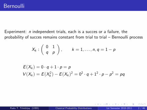
Bernoulli

Experiment: n independent trials, each is a succes or a failure, theprobability of succes remains constant from trial to trial �Bernoulli process

Xk :�0 1q p

�, k = 1, . . . , n, q = 1� p

E (Xk ) = 0 � q + 1 � p = pV (Xk ) = E (X

2k )� E (Xk )2 = 02 � q + 12 � p � p2 = pq


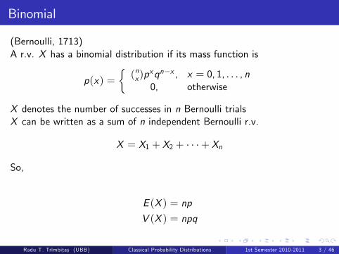
Binomial

(Bernoulli, 1713)A r.v. X has a binomial distribution if its mass function is

p(x) =�(nx)p

xqn�x , x = 0, 1, . . . , n0, otherwise

X denotes the number of successes in n Bernoulli trialsX can be written as a sum of n independent Bernoulli r.v.

X = X1 + X2 + � � �+ Xn

So,

E (X ) = np

V (X ) = npq


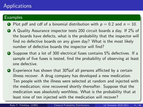
Applications

Examples1 Plot pdf and cdf of a binomial distribution with p = 0.2 and n = 10.2 A Quality Assurance inspector tests 200 circuit boards a day. If 2% ofthe boards have defects, what is the probability that the inspector will�nd no defective boards on any given day? What is the most likelynumber of defective boards the inspector will �nd?

3 Suppose that a lot of 300 electrical fuses contains 5% defectives. If asample of �ve fuses is tested, �nd the probability of observing at leastone defective.

4 Experience has shown that 30%of all persons a icted by a certainillness recover. A drug company has developed a new medication.Ten people with the illness were selected at random and injected withthe medication; nine recovered shortly thereafter. Suppose that themedication was absolutely worthless. What is the probability that atleast nine of ten injected with the medication will recover?


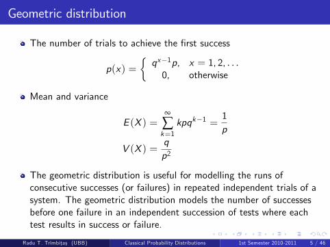
Geometric distribution

The number of trials to achieve the �rst success

p(x) =�qx�1p, x = 1, 2, . . .0, otherwise

Mean and variance

E (X ) =∞

∑k=1

kpqk�1 =1p

V (X ) =qp2

The geometric distribution is useful for modelling the runs ofconsecutive successes (or failures) in repeated independent trials of asystem. The geometric distribution models the number of successesbefore one failure in an independent succession of tests where eachtest results in success or failure.


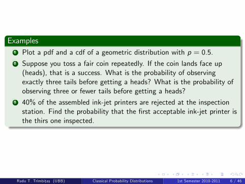
Examples1 Plot a pdf and a cdf of a geometric distribution with p = 0.5.2 Suppose you toss a fair coin repeatedly. If the coin lands face up(heads), that is a success. What is the probability of observingexactly three tails before getting a heads? What is the probability ofobserving three or fewer tails before getting a heads?

3 40% of the assembled ink-jet printers are rejected at the inspectionstation. Find the probability that the �rst acceptable ink-jet printer isthe thirs one inspected.


Negative binomial distribution

X has a negative binomial distribution with parameters r 2 N andp 2 (0, 1) if its mass function is

f (x jr , p) =�r + x � 1

x

�prqx , x 2 N

It can be thought of as modelling the total number of failures thatoccured before the nth success

E (X ) =rqp

V (X ) =rqp2

Sometimes X is considered to be the number of trials to amass atotal o r successes

P(X = n) =�n� 1r � 1

�prqn�r , n = r , r + 1, . . .


Applications

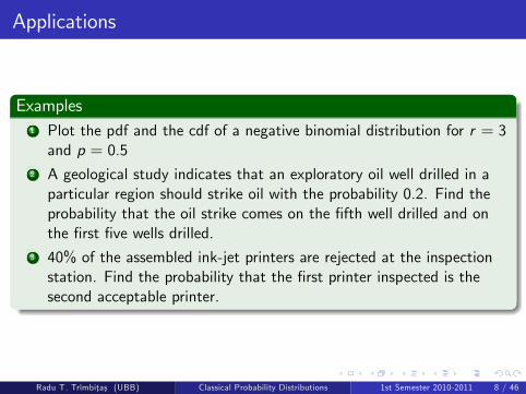
Examples1 Plot the pdf and the cdf of a negative binomial distribution for r = 3and p = 0.5

2 A geological study indicates that an exploratory oil well drilled in aparticular region should strike oil with the probability 0.2. Find theprobability that the oil strike comes on the �fth well drilled and onthe �rst �ve wells drilled.

3 40% of the assembled ink-jet printers are rejected at the inspectionstation. Find the probability that the �rst printer inspected is thesecond acceptable printer.


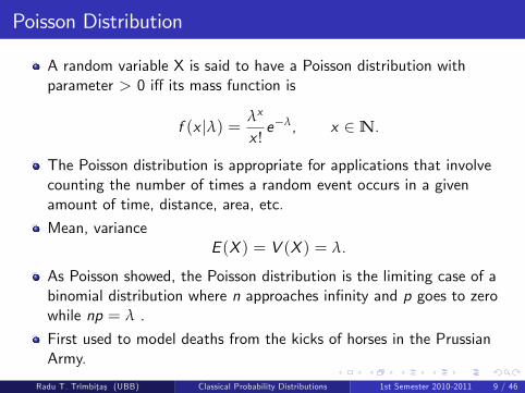
Poisson Distribution

A random variable X is said to have a Poisson distribution withparameter > 0 i¤ its mass function is

f (x jλ) = λx

x !e�λ, x 2 N.

The Poisson distribution is appropriate for applications that involvecounting the number of times a random event occurs in a givenamount of time, distance, area, etc.

Mean, varianceE (X ) = V (X ) = λ.

As Poisson showed, the Poisson distribution is the limiting case of abinomial distribution where n approaches in�nity and p goes to zerowhile np = λ .

First used to model deaths from the kicks of horses in the PrussianArmy.


Applications I

1 Plot the pdf and the cdf of a Poisson distribution for λ = 5.2 Suppose that a random system of police patrol is devised so that apatrol o¢ cer may visit a given beat location Y = 0, 1, 2, . . . times perhalf-hour period, with each location being visited an average of onceper time period. Assume that Y possesses, approximately, a Poissonprobability distribution. Calculate the probability that the patrolo¢ cer will miss a given location during a half-hour period. What isthe probability that it will be visited once? Twice? At least once?

3 A computer hard disk manufacturer has observed that �aws occurrandomly in the manufacturing process at the average rate of two�aws in a 4 Gb hard disk and has found this rate to be acceptable.What is the probability that a disk will be manufactured with nodefects?


Applications II

4 Consider a Quality Assurance department that performs random testsof individual hard disks. Their policy is to shut down themanufacturing process if an inspector �nds more than four badsectors on a disk. What is the probability of shutting down theprocess if the mean number of bad sectors (λ) is two?

5 A repair person is �beeped� each time there is a call service. Thenumber of beeps is Poisson with λ = 2 per hour. Find the probabilityof three beeps in the next hour, and the probability of more thanthree beeps i an 1-hour period.

6 The lead time demand in an inventory system is the accumulation ofdemand for an item at which an order is placed until the order isreceived

L =T

∑i=1Di ,


Applications III

where L is the lead-time demand, Di is the demand during the ithtime period, and T is the number of time periods during the leadtime. Both Di and T may be random variables. An inventorymanager desires that the probability of a stockout not exceed acertain fraction (e.g. 5%) during the lead time. The roerder point isthe level of inventory at which a new order is placed. Assume that thelead-time demand is poisson distributed with a mean of λ = 10 unitsand that a 95% protection of a stockout is desired. That is, �nd thesmallest x such that the probability that the lead-time demand doesnot exceed x is � 95%.


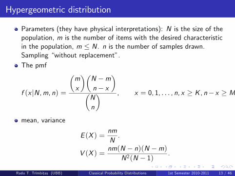
Hypergeometric distribution

Parameters (they have physical interpretations): N is the size of thepopulation, m is the number of items with the desired characteristicin the population, m � N. n is the number of samples drawn.Sampling �without replacement�.The pmf

f (x jN,m, n) =

�mx

��N �mn� x

��Nn

� , x = 0, 1, . . . , n, x � K , n� x � M�K .

mean, variance

E (X ) =nmN.

V (X ) =nm(N � n)(N �m)

N2(N � 1) .


Applications

1 Plot the pdf and the cdf of an experiment taking 20 samples from agroup of 1000 where there are 50 items of the desired type.

2 Suppose you have a lot of 100 �oppy disks and you know that 20 ofthem are defective. What is the probability of drawing 0 through 5defective �oppy disks if you select 10 at random? What is theprobability of drawing zero to two defective �oppies if you select 10 atrandom?

3 Suppose you are the Quality Assurance manager for a hard diskmanufacturer. The production line turns out disks in batches of1,000. You want to sample 50 disks from each batch to see if theyhave defects. You want to accept 99% there are no more than 10defective disks in the batch. What is the maximum number ofdefective disks should you allow in your sample of 50?


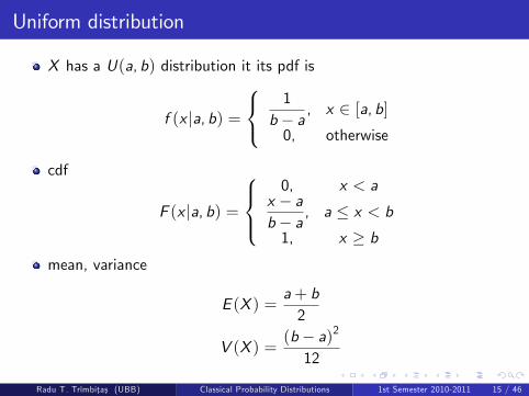
Uniform distribution

X has a U(a, b) distribution it its pdf is

f (x ja, b) =

8<:1

b� a , x 2 [a, b]0, otherwise

cdf

F (x ja, b) =

8><>:0, x < a

x � ab� a , a � x < b1, x � b

mean, variance

E (X ) =a+ b2

V (X ) =(b� a)2

12


Applications

1 Plot the graphs of pdf and cdf of a U [0, 1] distribution.2 What is the probability that an observation from a uniformdistribution with a = �1 and b = 1 will be less than 0.75?

3 What is the 99th percentile of the uniform distribution between -1and 1?

4 A bus arrives every 20 minutes at a speci�ed stop beginning at 6:40A.M. and continuing until 8:40 A.M. A certain passenger does notknow the schedule, but arrives randomly (uniformly distributed)between 7:00 A.M. and 7:30 A.M. every morning. What is theprobability that the passenger waits more than 5 minutes for a bus.


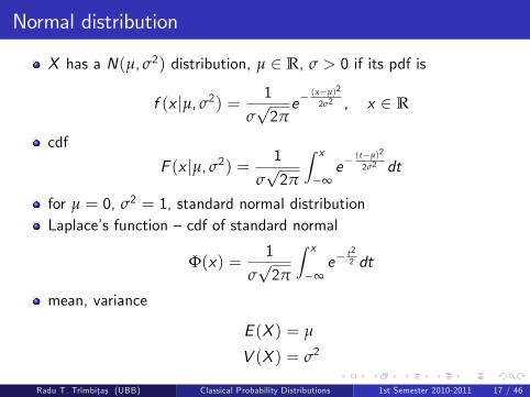
Normal distribution

X has a N(µ, σ2) distribution, µ 2 R, σ > 0 if its pdf is

f (x jµ, σ2) = 1

σp2πe�

(x�µ)2

2σ2 , x 2 R

cdf

F (x jµ, σ2) = 1

σp2π

Z x

�∞e�

(t�µ)2

2σ2 dt

for µ = 0, σ2 = 1, standard normal distributionLaplace�s function �cdf of standard normal

Φ(x) =1

σp2π

Z x

�∞e�

t22 dt

mean, variance

E (X ) = µ

V (X ) = σ2


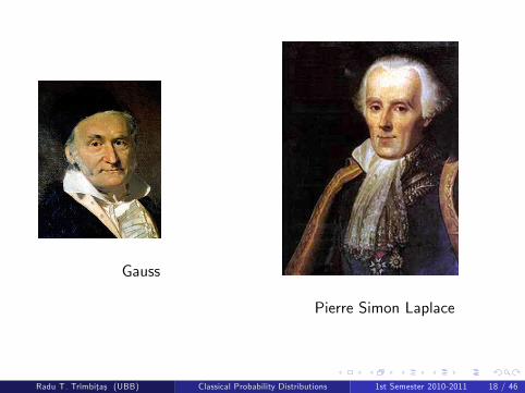
Gauss

Pierre Simon Laplace


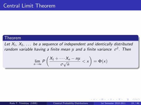
Central Limit Theorem

TheoremLet X1, X2, . . . be a sequence of independent and identically distributedrandom variable having a �nite mean µ and a �nite variance σ2. Then

limn!∞

P�X1 + � � �Xn � nµ

σpn

< x�= Φ(x)


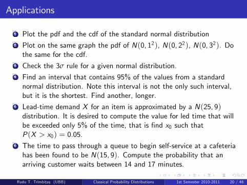
Applications

1 Plot the pdf and the cdf of the standard normal distribution2 Plot on the same graph the pdf of N(0, 12), N(0, 22), N(0, 32). Dothe same for the cdf.

3 Check the 3σ rule for a given normal distribution.4 Find an interval that contains 95% of the values from a standardnormal distribution. Note this interval is not the only such interval,but it is the shortest. Find another, longer.

5 Lead-time demand X for an item is approximated by a N(25, 9)distribution. It is desired to compute the value for led time that willbe exceeded only 5% of the time, that is �nd x0 such thatP(X > x0) = 0.05.

6 The time to pass through a queue to begin self-service at a cafeteriahas been found to be N(15, 9). Compute the probability that anarriving customer waits between 14 and 17 minutes.


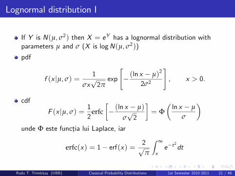
Lognormal distribution I

If Y is N(µ, σ2) then X = eY has a lognormal distribution withparameters µ and σ (X is logN(µ, σ2))

pdf

f (x jµ, σ) = 1

σxp2π

exp

"� (ln x � µ)2

2σ2

#, x > 0.

cdf

F (x jµ, σ) = 12

erfc�� (ln x � µ)

σp2

�= Φ

�ln x � µ

σ

�unde Φ este functia lui Laplace, iar

erfc(x) = 1� erf(x) = 2pπ

Z ∞

xe�t

2dt


Lognormal distribution II

Mean, variance

E (X ) = eµ+σ2/2

V (X ) = e2µ+σ2�eσ2 � 1

�If the mean and the variance are known to be µL and σ2L , respectively,then

µ = ln

0@ µLqµ2L + σ2L

1Aσ2 = ln

�µ2L + σ2L

µ2L

�.


Lognormal distribution III

median, mode

Mode(X ) = eµ�σ2

Median(X ) = eµ

A variable might be modeled as log-normal if it can be thought of asthe multiplicative product of many independent random variableseach of which is positive. For example, in �nance, a long-termdiscount factor can be derived from the product of short-termdiscount factors. In wireless communication, the attenuation causedby shadowing or slow fading from random objects is often assumed tobe log-normally distributed. Economists often model the distributionof income using a lognormal distribution.


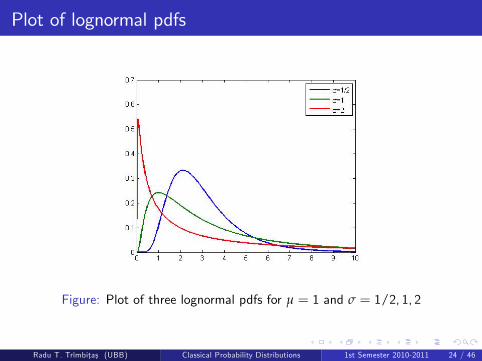
Plot of lognormal pdfs

Figure: Plot of three lognormal pdfs for µ = 1 and σ = 1/2, 1, 2


Applications

1 Suppose the income of a family of four in the United States follows alognormal distribution with µ = ln(20, 000$) and σ2 = 1. Plot theincome density. What is the probability that the income be largerthan 60000$.

2 The rate of return on a volatile investment is modeled as having alognormal distribution with mean 20% and standard deviation 5%.Compute the parameters for the lognormal distribution.


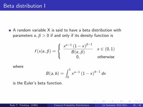
Beta distribution I

A random variable X is said to have a beta distribution withparameters α, β > 0 if and only if its density function is

f (x jα, β) =

8<: xα�1 (1� x)β�1

B(α, β)x 2 (0, 1)

0, otherwise

where

B(a, b) =Z 1

0xa�1 (1� x)b�1 dx

is the Euler�s beta function.


Beta distribution II

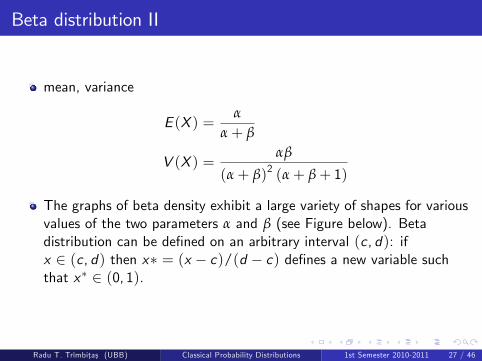
mean, variance

E (X ) =α

α+ β

V (X ) =αβ

(α+ β)2 (α+ β+ 1)

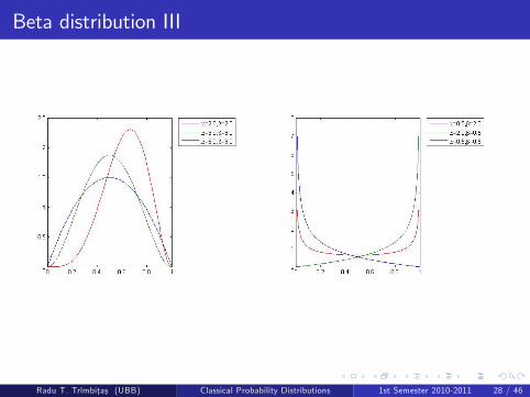
The graphs of beta density exhibit a large variety of shapes for variousvalues of the two parameters α and β (see Figure below). Betadistribution can be de�ned on an arbitrary interval (c , d): ifx 2 (c , d) then x� = (x � c)/(d � c) de�nes a new variable suchthat x� 2 (0, 1).


Beta distribution III


Applications I

1 A gasoline wholesale distributor has bulk storage tanks that hold �xedsupplies and are �lled every Monday. Of interest to the wholesaler isthe proportion of this supply that is sold during the week. Over manyweeks of observation, the distributor that this proportion could bemodelled by a beta distribution with α = 4 and β = 2. Find theprobability that the wholesaler will sent at least 90% of her stock in agiven week.

2 Rule of succession. A classic application of the beta distribution isthe rule of succession, introduced in the 18th century by Pierre-SimonLaplace in the course of treating the sunrise problem. It states that,given s successes in n conditionally independent Bernoulli trials withprobability p, that p should be estimated as s+1n+2 . This estimate maybe regarded as the expected value of the posterior distribution over p,namely Beta(s + 1, n� s + 1), which is given by Bayes�rule if one


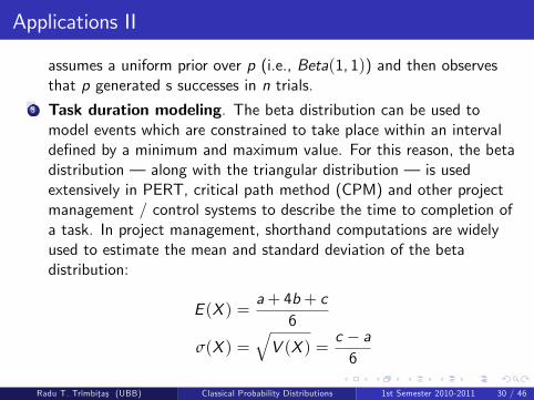
Applications II

assumes a uniform prior over p (i.e., Beta(1, 1)) and then observesthat p generated s successes in n trials.

3 Task duration modeling. The beta distribution can be used tomodel events which are constrained to take place within an intervalde�ned by a minimum and maximum value. For this reason, the betadistribution � along with the triangular distribution � is usedextensively in PERT, critical path method (CPM) and other projectmanagement / control systems to describe the time to completion ofa task. In project management, shorthand computations are widelyused to estimate the mean and standard deviation of the betadistribution:

E (X ) =a+ 4b+ c

6

σ(X ) =qV (X ) =

c � a6


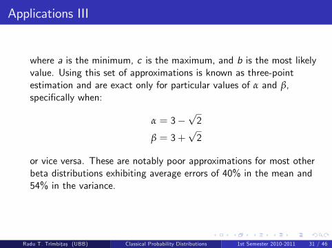
Applications III

where a is the minimum, c is the maximum, and b is the most likelyvalue. Using this set of approximations is known as three-pointestimation and are exact only for particular values of α and β,speci�cally when:

α = 3�p2

β = 3+p2

or vice versa. These are notably poor approximations for most otherbeta distributions exhibiting average errors of 40% in the mean and54% in the variance.


Triangular distribution I

X has a triangular distribution with parameters a, b, c , a � b � c ifits pdf is

f (x ja, b, c) =

8>>>><>>>>:2(x � a)

(b� a)(c � a) , x 2 [a, b]2(c � x)

(c � b)(c � a) , x 2 (b, c ]0, elsewhere

mean, mode

E (X ) =a+ b+ c

3Mode = b = 3E (X )� (a+ c)


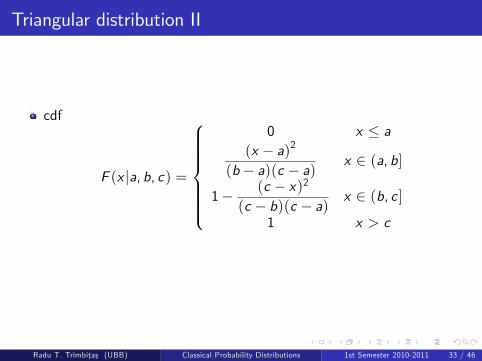
Triangular distribution II

cdf

F (x ja, b, c) =

8>>>>>><>>>>>>:

0 x � a(x � a)2

(b� a)(c � a) x 2 (a, b]

1� (c � x)2(c � b)(c � a) x 2 (b, c ]

1 x > c


Applications I

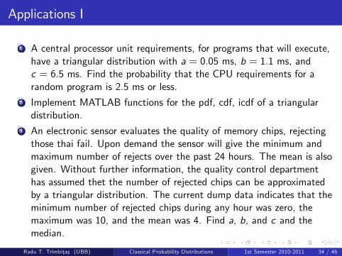
1 A central processor unit requirements, for programs that will execute,have a triangular distribution with a = 0.05 ms, b = 1.1 ms, andc = 6.5 ms. Find the probability that the CPU requirements for arandom program is 2.5 ms or less.

2 Implement MATLAB functions for the pdf, cdf, icdf of a triangulardistribution.

3 An electronic sensor evaluates the quality of memory chips, rejectingthose thai fail. Upon demand the sensor will give the minimum andmaximum number of rejects over the past 24 hours. The mean is alsogiven. Without further information, the quality control departmenthas assumed thet the number of rejected chips can be approximatedby a triangular distribution. The current dump data indicates that theminimum number of rejected chips during any hour was zero, themaximum was 10, and the mean was 4. Find a, b, and c and themedian.


Applications II

4 Find conditions on a, b, c such that mean, mode and median beequal.

5 Find the variance and the median of a Triang(a, b, c) r.v.


Exponential distribution I

X is said to be exponential distributed with parameter λ > 0 if its pdfis

f (x) =�

λe�λx , x � 00, otherwise

cdf

F (x) =�

0 x < 01� e�λx , x � 0

mean, variance, median

E (X ) =1λ

V (X ) =1

λ2

Me(X ) =ln 2λ


Exponential distribution II

variant (in statistical packages)

f (x) =

( 1λe�

xλ , x � 0

0, otherwise

E (X ) = λ, V (X ) = λ2

Exponential distribution models interarrival times when arrivals arecompletely random and to model service time that are highly variable.In this instances λ is a rate: arrivals per hour or services per minute

model the lifetime of a component that fails catastrophically(instantaneously), luch as a light bulb; λ is the failure rate.


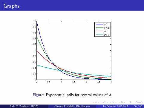
Graphs

Figure: Exponential pdfs for several values of λ


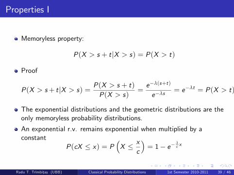
Properties I

Memoryless property:

P(X > s + tjX > s) = P(X > t)

Proof

P(X > s+ tjX > s) = P(X > s + t)P(X > s)

=e�λ(s+t)

e�λs = e�λt = P(X > t)

The exponential distributions and the geometric distributions are theonly memoryless probability distributions.

An exponential r.v. remains exponential when multiplied by aconstant

P(cX � x) = P�X � x

c

�= 1� e� λ

c x


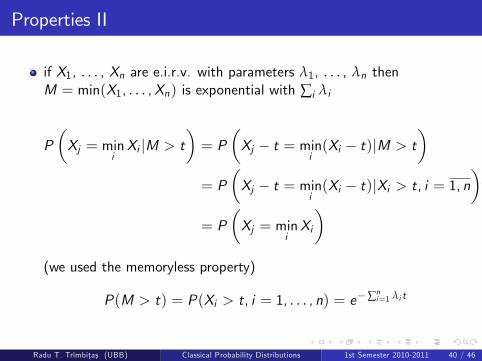
Properties II

if X1, . . . , Xn are e.i.r.v. with parameters λ1, . . . , λn thenM = min(X1, . . . ,Xn) is exponential with ∑i λi

P�Xj = min

iXi jM > t

�= P

�Xj � t = min

i(Xi � t)jM > t

�= P

�Xj � t = min

i(Xi � t)jXi > t, i = 1, n

�= P

�Xj = min

iXi

�(we used the memoryless property)

P(M > t) = P(Xi > t, i = 1, . . . , n) = e�∑ni=1 λi t


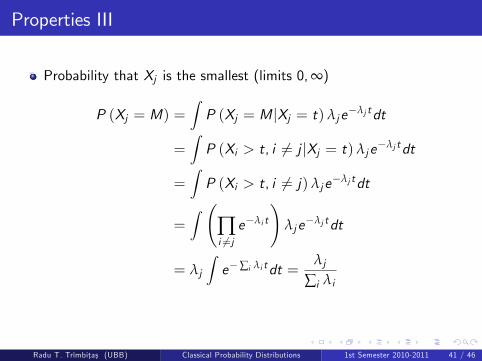
Properties III

Probability that Xj is the smallest (limits 0,∞)

P (Xj = M) =ZP (Xj = M jXj = t) λje�λj tdt

=ZP (Xi > t, i 6= j jXj = t) λje�λj tdt

=ZP (Xi > t, i 6= j) λje�λj tdt

=Z

∏i 6=je�λi t

!λje�λj tdt

= λj

Ze�∑i λi tdt =

λj

∑i λi


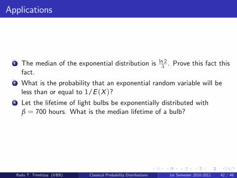
Applications

1 The median of the exponential distribution is ln 2λ . Prove this fact thisfact.

2 What is the probability that an exponential random variable will beless than or equal to 1/E (X )?

3 Let the lifetime of light bulbs be exponentially distributed withβ = 700 hours. What is the median lifetime of a bulb?


Weibull distribution I

X has a Weibull distribution with parameters ν 2 R, α > 0, β > 0 ifits pdf is

f (x jν, α, β) =

8><>:β

α

�x � ν

α

�β�1exp

"��x � ν

α

�β#, x � ν

0, otherwise

cdf

F (x) =

8><>:0, x < ν

1� exp"��x � ν

α

�β#, x � ν

ν - location parameter, α - scale parameter, β - shape parameter

ν = 0 two parameter Weibull

ν = 0, β = 1, exponential with parameter λ = 1α


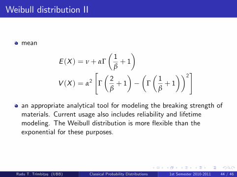
Weibull distribution II

mean

E (X ) = ν+ αΓ�1β+ 1�

V (X ) = α2

"Γ�2β+ 1��

Γ�1β+ 1��2#

an appropriate analytical tool for modeling the breaking strength ofmaterials. Current usage also includes reliability and lifetimemodeling. The Weibull distribution is more �exible than theexponential for these purposes.


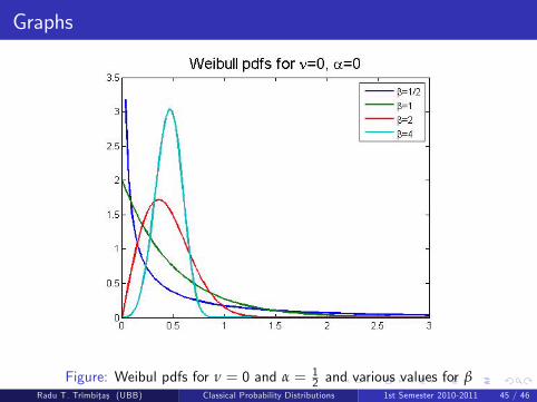
Graphs

Figure: Weibul pdfs for ν = 0 and α = 12 and various values for β


Applications

1 Reproduce Figure 3. Plot cdfs for the same distributions.2 Find the formula for the median of a Weibull distribution.3 The time to failure for a component screen is known to have a Weibulldistribution with ν = 0, β = 1/3, and α = 200 hours. Find the mean,the variance and the probability that a unit fails before 2000 hours.

4 The time it takes for an aircraft to land and clear the runaway at amajor international airport has a Weibull distribution with ν = 1.34minutes, β = 0.5 and α = 0.04 minutes. Find the probability that anincoming airpalne will take more than 1.5 minutes to land and clerthe runaway.


Documents

Classical Probability Distributions - Babeș-Bolyai Universitymath.ubbcluj.ro/~tradu/classicalpd.pdf · Classical Probability Distributions ... Radu T. Trîmbi‚ta‚s (UBB) Classical