1

Classical Theory of Harmonic Crystals

HARMONIC APPROXIMATION The Hamiltonian of the crystal is expressed in terms of the kinetic energies of atoms and the potential

energy.

∑

In calculating the potential energy, we use the assumptions:

1. The mean equilibrium position of each ion is a Bravais lattice site R.

2. Ions oscillate about their equilibrium positions with amplitudes small compared with the

interionic spacing.

The total potential of the crystal is the sum of all pair potentials:

∑

Use Taylor expansion:

∑

∑( )

∑( )

The first term is the equilibrium potential energy:

∑

∑

The second term in equation (4) vanishes since the coefficient of each displacement is simply the

negative of the sum of all forces acting on an atom at its equilibrium position:

∑

The third term is the harmonic contribution to the potential energy:

2

∑ ∑[

]

[ ]

Equation (7) can be rewritten in a more compact form:

∑∑

This is a more useful form since the coefficients Dμν cannot be always represented by pair potentials

(except in the simple case of crystals of noble gases).

ADIABATIC APPROXIMATION In ionic crystals, the long-range coulomb interaction makes it difficult to calculate the coefficients Dμν. In

covalent crystals and metals, the ionic motion is coupled to the motion of the valence electrons, the

wave functions of which depend on the positions of the ion cores. The adiabatic approximation is based

on the fact that valence electrons move much faster than the ion cores (108 cm/s vs. 105 cm/s). Thus the

ion cores can be considered instantaneously at rest with displacements u(R) from their equilibrium

positions, and the electron configuration is calculated and the additional energy due to electron-ion

interactions computed and added. This is a difficult problem, and more practically, the coefficients can

be regarded as empirical parameters to be determined by experiment.

SPECIFIC HEAT To determine the specific heat per unit volume for a solid, we first calculate its energy density. Using

the canonical ensemble, this is given by:

Here β = kBT, and Q is the partition function given by the integral over phase space:

∫

The energy H of the system is given by equations (1) and (8). The partition function is then given by:

∫∏

[ (∑

∑

)]

Change of variables:

3

With this definition, equation (11) becomes:

∫∏

[ (∑

∑

)]

Thus equation (9) yields:

The specific heat at constant volume (constant ionic number per unit volume) is then:

The specific heat per ion is simply 3kB, which is the famous Dulong-Petit law. The molar specific heat for

a monatomic solid is given by:

Note: Naively speaking, the expansion of the solid due to crystal vibrations results from an-harmonic

contributions to the energy which are very small (and ignored in our previous analysis). Ignoring such

contributions leaves the volume of the solid constant, and the specific heat at constant pressure is

identical to that at constant volume. An-harmonic contributions become more significant with

increasing temperature due to the increase of vibrational amplitudes, and the consequent deviation of

the crystal potential from the harmonic form. At room temperature, the specific heat at constant

pressure is within 1% of the specific heat at constant volume. The difference between the two specific

heats becomes much less than 1% at low temperatures.

The experimental specific heat of a typical monatomic solid (such as argon, krypton, or xenon) is shown

in Fig. 1. The specific heat approaches the Dulong-Petit value at temperatures above 100 K. The

deviation of the high temperature experimental value

from the theoretical value can be explained classically as

due to failure of the harmonic approximation in this

temperature range, since neglected an-harmonic effects

become appreciable. However, at low temperatures

where the harmonic approximation is expected to hold

quite well, the specific heat drops sharply toward zero,

which indicates the inadequacy of classical treatment.

However, before resorting to a quantum theory of

lattice vibrations, we can make use of the classical 20 40 60 80

Fig. 1: Measured specific heat for Ar solid

CV (

J/m

ole

.K)

30

20

10

T (K)

4

theory due to the resemblance of the quantum energies to the classical energies of the 3N modes of

vibrations of N oscillators in a harmonic crystal as determined using the theory of small oscillations. The

only modification we make is the replacement of the energy (nhν) of a classical vibrational mode by the

correct phonon quantum energy (n + ½)hν. Therefore, we next consider the analysis of classical normal

modes of lattice vibrations.

ONE DIMENSINAL MONATOMIC LATTICE First consider N ions of mass M each, positioned along a line at the equilibrium positions na, and vibrate

with small amplitudes about these positions. In the case of nearest neighbor interactions, equation (7)

reduces to the form:

∑ ∑

|

Notice that each term in the sum occurs twice due to the sum over m. This equation therefore reduces

to the form:

∑

The force constant K is the second derivative of the interaction potential of two adjacent ions. The

equations of motion are constructed from the potential in (17):

[( ) ( )] [ ]

Since the number of ions is very large, the end points can be ignored, and we can use Born-von Karman

boundary conditions for mathematical convenience, and thus in solving (18) we use:

We look for propagating wave solution of (18) of the form:

The periodic boundary conditions in (19) indicate that:

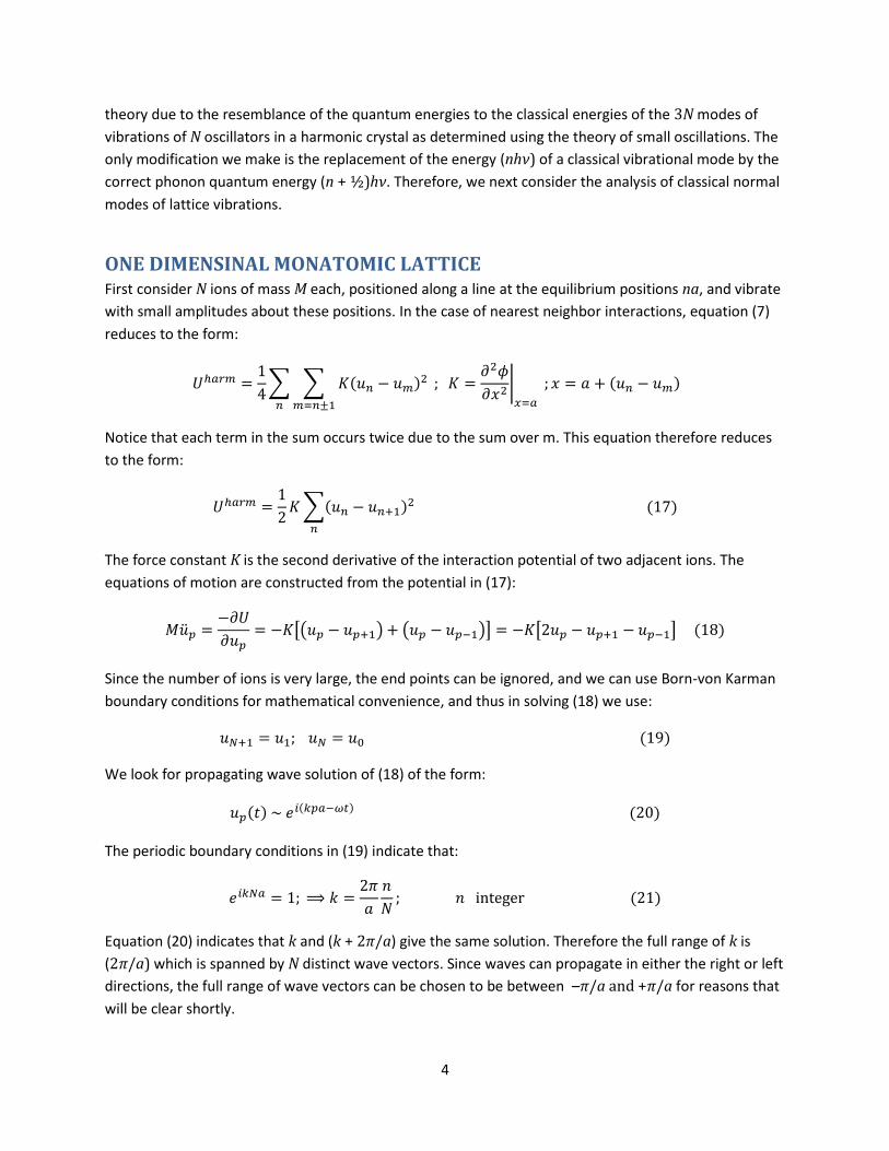
Equation (20) indicates that k and (k + 2π/a) give the same solution. Therefore the full range of k is

(2π/a) which is spanned by N distinct wave vectors. Since waves can propagate in either the right or left

directions, the full range of wave vectors can be chosen to be between –π/a and +π/a for reasons that

will be clear shortly.

5

With the solution given by (20), the equation of motion (18) reads:

[ ] [ ]

[ ]

Equation (22) is used to determine the normal mode frequencies of the chain, which are given by:

√ [ ]

√

| (

)| | (

)|

Notice that ω(– k) = ω(k), thus the above mentioned choice for the zone boundaries is valid and

displays the symmetry of the dispersion relation. There are N normal modes corresponding to the N

distinct values of k. The dispersion relation (23) is shown in Fig. 2. The physical motion of the chain is

described by:

{

}

These two solutions differ in phase by π/2. The

general solution is determined by specifying N initial

positions of the ions, and their initial velocities. The

phase and group velocities of propagating waves are:

(

)

The group velocity starts with a constant value near

the origin (the long wavelength limit) and decreases to

zero at the zone boundaries when the wavelength

becomes comparable with the interionic spacings. In the long wavelength limit the phase velocity and

group velocity are equal (= aω0/2).

The number of modes in the frequency range dω is given in terms of density of normal mode

frequencies by:

Here k varies between 0 and π/a. The factor 2 is due to the fact that each frequency corresponds to 2- k

points (–k and +k). We therefore obtain the density of normal mode frequencies as:

(

)

0

Fig. 2: Dispersion curve for a

monatomic linear chain. The straight

lines represent the curve ω = ck.

ω(k)

𝜔

k π/a –π/a

6

Using equation (25) and (23) we obtain:

√

√

(

)

√(

)

Combining these last two equations we obtain:

[ ]

Fig. 3 shows the density of normal modes. Notice that in the long wavelength limit the density of modes

is constant, and then starts rising with frequency, and diverges at the maximum frequency.

ONE DIMENSINAL DIATOMIC LATTICE In this chain, the two ions per primitive cell are identical and situated at positions na and na + d. If d <

a/2, then the interaction between the two ions separated by d is different from that between two ions

separated by (d – a), leading to two different force constants. Fig. 4 shows the chain in this case.

The harmonic potential energy for the chain, assuming nearest neighbor interactions only, is:

∑[ ]

∑[ ]

In this equation we have the following assignments:

un the displacement of the first ion in the basis with equilibrium position at na.

sn the displacement of the second ion in the basis with equilibrium position at na + d.

un+1 the displacement of the first ion in the basis with equilibrium position at (n+ 1)a.

0

Fig. 3: Density of normal

modes for a monatomic linear

chain

G(ω)

ω ω0

d

a na (n+1) a

Fig. 4: One-dimensional diatomic chain

7

K1 the force constant between ions separated by d in the same cell.

K2 the force constant between ions separated by a – d in adjacent cells.

The equations of motion for the two basis ions are:

[ ] [ ]

[ ] [ ]

We seek solutions of equation (31) of the form:

Born-von Karman boundary conditions again give the N values of k given by equation (21).

Substituting (32) into (31) leads to the two coupled equations:

[ ] [ ]

[ ] [ ]

Solution is the obtained by setting the determinant of the coefficients A and B equal to zero:

[ ] [

] [ ]

Solving this equation gives:

√

Substituting these values into (33) gives the ratios of the amplitudes:

[ ] √

| |

8

For each k value, there are two characteristic

frequencies, giving a total of 2N normal modes

characteristic of the 2N degrees of freedom. The

two branches of the dispersion curve are shown

in Fig. 5. The acoustic branch starts from zero

frequency and goes up to a maximum frequency

at the zone boundary as shown. This branch

exhibits characteristics similar to sound waves in

the long wavelength limit. The optical branch

starts from a maximum frequency and goes

down to a minimum frequency at the zone

boundary. This minimum frequency, however, is

higher than the maximum frequency of the

acoustic branch, leading to a band gap at the

zone boundary. In the long wavelength limit, the

optical modes can interact with electromagnetic

fields, and give rise to the characteristic optical properties of ionic crystals.

1. Long wavelength limit: k ≪ π/a:

√

√

In this limit, ions in neighboring cells move in phase as indicated by equation (32). In the acoustic branch

(Fig. 6) the two ions in a cell also move in phase according to equation (37), resulting in zero frequency at

k = 0 (the translational mode).

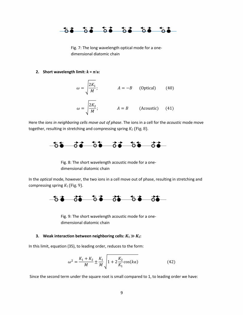
In the optical branch, however, the two ions in a cell move out of phase (Fig. 7), resulting in stretching

and compressing both springs consistent with (38).

0

Fig. 5: Dispersion curves for a

diatomic linear chain

ω(k)

𝐾 𝑀

k

π/a –π/a

𝐾 𝑀

𝐾 𝐾 𝑀

Fig. 6: The long wavelength acoustic mode for a one-

dimensional diatomic chain

9

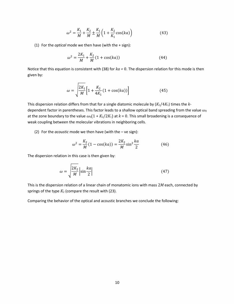
2. Short wavelength limit: k = π/a:

√

√

Here the ions in neighboring cells move out of phase. The ions in a cell for the acoustic mode move

together, resulting in stretching and compressing spring K2 (Fig. 8).

In the optical mode, however, the two ions in a cell move out of phase, resulting in stretching and

compressing spring K1 (Fig. 9).

3. Weak interaction between neighboring cells: K1 ≫ K2:

In this limit, equation (35), to leading order, reduces to the form:

√

Since the second term under the square root is small compared to 1, to leading order we have:

Fig. 7: The long wavelength optical mode for a one-

dimensional diatomic chain

Fig. 8: The short wavelength acoustic mode for a one-

dimensional diatomic chain

Fig. 9: The short wavelength acoustic mode for a one-

dimensional diatomic chain

10

(

)

(1) For the optical mode we then have (with the + sign):

Notice that this equation is consistent with (38) for ka = 0. The dispersion relation for this mode is then

given by:

√

[

]

This dispersion relation differs from that for a single diatomic molecule by (K2/4K1) times the k-

dependent factor in parentheses. This factor leads to a shallow optical band spreading from the value ω0

at the zone boundary to the value ω0(1 + K2/2K1) at k = 0. This small broadening is a consequence of

weak coupling between the molecular vibrations in neighboring cells.

(2) For the acoustic mode we then have (with the – ve sign):

The dispersion relation in this case is then given by:

√

|

|

This is the dispersion relation of a linear chain of monatomic ions with mass 2M each, connected by

springs of the type K2 (compare the result with (23).

Comparing the behavior of the optical and acoustic branches we conclude the following:

11

a. In the acoustic mode the basis ions in a

primitive cell move in phase, and the

dynamics of crystal vibration is dominated

by intercellular interactions (between the

cells).

b. In the optical branch the dynamics of

crystal vibration is dominated by

intracellular molecular vibrational mode

within each primitive cell, which is

broadened by intercellular weak

interactions.

This behavior is similar to the shallow bands

obtained in the tight binding model for electronic

states as shown in Fig. 10.

Generalization to three dimensions The modes discussed above are the longitudinal modes

of vibrations. If transverse motion is investigated, it is

found to produce similar transverse modes with

shallower bands. Crystal symmetries may lead to

degeneracies of these bands. The general dispersion

curves for a crystal with two ions per primitive cell in a

general direction of k (which is not a high symmetry

direction) is shown in Fig. 11 in the case of strong

intracellular interactions compared to intercellular

interactions.

0

Fig. 10: Dispersion curves for a

diatomic linear chain in tight binding

limit

ω(k)

𝐾 𝑀

k

π/a –π/a

𝐾 𝑀

𝐾 𝐾 𝑀

0

Fig. 11: Dispersion curves for a

diatomic linear chain in tight binding

limit

ω(k)

k