Embed Size (px)
Citation preview
Classification in Networked Data0:A toolkit and a univariate case study
Sofus A. Macskassy [email protected]
Fetch Technologies, Inc.2041 Rosecrans AvenueEl Segundo, CA 90254
Foster Provost [email protected] .EDU
New York University44 W. 4th StreetNew York, NY 10012
Editor:
Abstract
This paper presents NetKit, a modular toolkit for classification in networked data, and a case-study of its application to networked data used in prior machine learning research. We considerwithin-network classification: entities whose classes are to be estimated are linked to entities forwhich the class is known. NetKit is based on a node-centric framework in which classifiers com-prise a local classifier, a relational classifier, and a collective inference procedure. Various existingnode-centric relational learning algorithms can be instantiated with appropriate choices for thesecomponents, and new combinations of components realize newalgorithms. The case study fo-cuses on univariate network classification, for which the only information used is the structure ofclass linkage in the network (i.e., only links and some classlabels). To our knowledge, no workpreviously has evaluated systematically the power of class-linkage alone for classification in ma-chine learning benchmark data sets. The results demonstrate that very simple network-classificationmodels perform quite well—well enough that they should be used regularly as baseline classifiersfor studies of learning with networked data. The simplest method (which performs remarkablywell) highlights the close correspondence between severalexisting methods introduced for differ-ent purposes—i.e., Gaussian-field classifiers, Hopfield networks, and relational-neighbor classi-fiers. The results also show that a small number of component combinations excel. In particular,there are two sets of techniques that are preferable in different situations, namely when few versusmany labels are known initially. We also demonstrate that link selection plays an important rolesimilar to traditional feature selection.
Keywords: relational learning, network learning, collective inference, collective classification,networked data
0. S.A. Macskassy and Provost, F.J., “Classification in Networked Data: A toolkit and a univariate case study” CeDERWorking Paper CeDER-04-08, Stern School of Business, New York University, NY, NY 10012. December 2004.Updated August 2006.

Report Documentation Page Form ApprovedOMB No. 0704-0188
Public reporting burden for the collection of information is estimated to average 1 hour per response, including the time for reviewing instructions, searching existing data sources, gathering andmaintaining the data needed, and completing and reviewing the collection of information. Send comments regarding this burden estimate or any other aspect of this collection of information,including suggestions for reducing this burden, to Washington Headquarters Services, Directorate for Information Operations and Reports, 1215 Jefferson Davis Highway, Suite 1204, ArlingtonVA 22202-4302. Respondents should be aware that notwithstanding any other provision of law, no person shall be subject to a penalty for failing to comply with a collection of information if itdoes not display a currently valid OMB control number.
1. REPORT DATE AUG 2006 2. REPORT TYPE
3. DATES COVERED 00-08-2006 to 00-08-2006
4. TITLE AND SUBTITLE Classification in Networked Data: A toolkit and a univariate case study
5a. CONTRACT NUMBER
5b. GRANT NUMBER
5c. PROGRAM ELEMENT NUMBER
6. AUTHOR(S) 5d. PROJECT NUMBER
5e. TASK NUMBER
5f. WORK UNIT NUMBER
7. PERFORMING ORGANIZATION NAME(S) AND ADDRESS(ES) Fetch Technologies Inc,2041 Rosecrans Avenue,El Segundo,CA,90254
8. PERFORMING ORGANIZATIONREPORT NUMBER
9. SPONSORING/MONITORING AGENCY NAME(S) AND ADDRESS(ES) 10. SPONSOR/MONITOR’S ACRONYM(S)
11. SPONSOR/MONITOR’S REPORT NUMBER(S)
12. DISTRIBUTION/AVAILABILITY STATEMENT Approved for public release; distribution unlimited
13. SUPPLEMENTARY NOTES
14. ABSTRACT
15. SUBJECT TERMS
16. SECURITY CLASSIFICATION OF: 17. LIMITATION OF ABSTRACT
18. NUMBEROF PAGES
49
19a. NAME OFRESPONSIBLE PERSON
a. REPORT unclassified
b. ABSTRACT unclassified
c. THIS PAGE unclassified
Standard Form 298 (Rev. 8-98) Prescribed by ANSI Std Z39-18
MACSKASSY AND PROVOST
1. Introduction
Networked datacontain interconnected entities for which inferences are to be made. For example,web pages are interconnected by hyperlinks, research papers are connected by citations, telephoneaccounts are linked by calls, possible terrorists are linked by communications. This paper is aboutwithin-network classification: entities for which the class is known are linked to entitiesfor whichthe class must be estimated. For example, telephone accounts previously determined to be fraudu-lent may be linked, perhaps indirectly, to those for which noassessment yet has been made.
Such networked data present both complications and opportunities for classification and ma-chine learning. The data are patently not i.i.d., which introduces bias to learning and inferenceprocedures (Jensen and Neville, 2002b). The usual careful separation of data into training and testsets is difficult, and more importantly, thinking in terms ofseparating training and test sets obscuresan important facet of the data: entities with known classifications can serve two roles. They act firstas training data and subsequently as background knowledge during inference. Relatedly, within-network inference allows models to use specific node identifiers to aid inference (see Section 3.4.2).
Network data allowcollective inference, meaning that various interrelated values can be inferredsimultaneously. For example, inference in Markov random fields (MRFs) (Dobrushin, 1968; Besag,1974; Geman and Geman, 1984) uses estimates of a node’s neighbor’s labels to influence the esti-mation of the node’s labels—and vice versa. Within-networkinference complicates such proceduresby pinning certain values, but also offers opportunities such as the application of network-flow al-gorithms to inference (see Section 3.4.1). More generally,network data allow the use of the featuresof a node’s neighbors, although that must be done with care toavoid greatly increasing estimationvariance and thereby error (Jensen et al., 2004).
To our knowledge there previously has been no large-scale, systematic experimental study ofmachine learning methods for within-network classification. A serious obstacle to undertaking sucha study is the scarcity of available tools and source code, making it hard to compare various method-ologies and algorithms. A systematic study is further hindered by the fact that many relational learn-ing algorithms can be separated into various sub-components; ideally the relative contributions ofthe sub-components and alternatives should be assessed.
As a main contribution of this paper, we introduce a network learning toolkit (NetKit-SRL)that enables in-depth, component-wise studies of techniques for statistical relational learning andclassification with networked data. We abstract prior, published methods into a modular frameworkon which the toolkit is based.1
NetKit is interesting for several reasons. First, various systems from prior work can be realizedby choosing particular instantiations for the different components. Besides simply making suchsystems available in a common platform, it allows one to compare and contrast the different systemson equal footing. Perhaps more importantly, the modularityof the toolkit broadens the design spaceof possible systems beyond those that have appeared in priorwork, either by mixing and matchingthe components of the prior systems, or by introducing new alternatives for components.
In the second half of the paper, we use NetKit to conduct a casestudy of within-network clas-sification in homogeneous, univariate networks, which are important both practically and scientifi-cally (as we discuss in Section 5). We compare various learning and inference techniques on twelvebenchmark data sets from four domains used in prior machine learning research. Beyond illustrating
1. NetKit-SRL, or NetKit for short, is written in Java 1.5 andis available as open source from the author’s web-page:http://www.research.rutgers.edu/˜sofmac/NetKit.html
2
CLASSIFICATION IN NETWORKED DATA
the value of the toolkit, the case provides systematic evidence that with networked data even univari-ate classification can be remarkably effective. One implication is that such methods should be usedas baselines against which to compare more sophisticated relational learning algorithms (Macskassyand Provost, 2003). One particular very simple and very effective technique highlights the closecorrespondence between several types of methods introduced for different purposes: “node-centric”methods, which focus on each node individually; methods that operate on the graph as a whole, e.g.,computing minimum cuts of different sorts; and classic connectionist methods. The case study alsoillustrates a bias/variance trade-off in networked classification, based on the principle of homophily(Blau, 1977; McPherson et al., 2001) (cf., assortativity (Newman, 2003) and relational autocorrela-tion (Jensen and Neville, 2002b)) and suggests network-classification analogues to feature selectionand active learning.
To further motivate and to put the rest of the paper into context, we start by reviewing some(published) applications of within-network inference. Section 3 describes the problem of networklearning more formally, introduces the modular framework,and surveys existing work on networkclassification. Section 4 describes NetKit. Then Section 5 covers the case study, including moti-vation for studying univariate network inference, the experimental methodology, data used, toolkitcomponents used, and the results and analysis.
2. Applications
The earliest work on classification in networked data arose in scientific applications, with the net-works based on regular grids of physical locations. Statistical physics introduced, for example, theIsing model (Ising, 1925) and the Potts model (Potts, 1952)), which were used to find minimumenergy configurations in physical systems with components exhibiting discrete states, such as mag-netic moments in ferromagnetic materials. Network-based techniques then saw wide application inimage processing (e.g., Besag (1986); Geman and Geman (1984)), where the networks were basedon grids of pixels, and also in spatial statistics Besag (1974).
More recent work concentrates on networks of arbitrary topology, for example, for the classi-fication of linked documents such as patents (Chakrabarti etal., 1998), scientific research papers(e.g., (Taskar et al., 2001; Lu and Getoor, 2003)), and web pages (e.g. (Neville et al., 2003; Lu andGetoor, 2003)). In a recent scientific application, Segal etal. (2003a,b) apply network classifica-tion (specifically, relational Markov networks (Taskar et al., 2002)) to protein interaction and geneexpression data. The protein interactions form a network over which inferences are drawn aboutpathways, i.e., sets of genes that coordinate to achieve a particular task. In computational linguis-tics network classification is applied to tasks such as the segmentation and labeling of text (e.g.,part-of-speech tagging (Lafferty et al., 2001)).
Business problems also have seen the application of network-based techniques. In fraud detec-tion entities to be classified as being fraudulent or legitimate are intertwined with those for whichclassifications are known. Fawcett and Provost (1997) discuss and experiment with so-called state-of-the-art fraud detection techniques, including a “dialed-digit monitor” that examines indirect (two-hop) connections to prior fraudulent accounts in the call network. Cortes et al. (2001) explicitly rep-resent and reason with accounts’ local network neighborhoods, for identifying telecommunicationsfraud. For making product recommendations, Huang et al. (2004) define a neighborhood of similarpeople for collaborative filtering and use graph-based message passing to draw inferences. Domin-gos and Richardson (2001) describe how an MRF-based technique could be used to estimate the
3
MACSKASSY AND PROVOST
best candidates for viral marketing. Hill et al. (2006) showthat statistical, network-based marketingtechniques can perform substantially (several times) better than traditional targeted marketing basedon demographics and prior purchase data.
With the exception of collaborative filtering, these business applications share the characteristicthat data are available on actual social networks, defined bydirect communications. Such networksplay an important role in counterterrorism and law enforcement: suspicious people may interactwith known malicious people. Macskassy and Provost (2005) present a network classification ap-proach for suspicion scoring in surveillance networks—i.e., ranking candidates by their estimatedlikelihood of being malicious (cf., (Galstyan and Cohen, 2005)). Neville et al. (2005) identified po-tential SEC violators from data provided by the National Association of Securities Dealers (NASD).Their models performed as well as or better than the handcrafted models currently in use at NASD.
Some other domains may not quite qualify as applications, but are interesting nevertheless.The Internet Movie Database contains rich relational and networked data such as actors, movies,producers, directors, etc. Jensen and Neville (2002a) predict whether a movie will make morethan two million dollars in its opening weekend, and others have followed (Neville et al., 2003;Macskassy and Provost, 2003, 2004). Bernstein et al. (2003)and Macskassy and Provost (2003,2004) have addressed the problem of categorizing what industry sector a given company belongsto using financial news to link companies based on whether they were mentioned in the same newsstory.
Finally, network classification approaches have seen elegant application on a problem that ini-tially does not present itself asnetworkclassification. In the problem setting for “transductive”inference (Vapnik, 1998a), a set of labeled data is presented together with a set of data for whichclassifications are made. Since data points can be linked into a network based on any similaritymeasure, any classification problem in the transductive setting can be treated as a (within-)networkclassification problem. We discuss this further below.
3. Network Classification and Learning
Traditionally, machine learning methods have treated entities as being independent, which makesit possible to infer class membership on an entity-by-entity basis. With networked data, the classmembership of one entity may have an influence on the class membership of a related entity. Fur-thermore, entities not directly linked may be related by chains of links, which suggests that it maybe beneficial to infer the class memberships of all entities simultaneously. Collective inferencing inrelational data (Taskar et al., 2002; Neville and Jensen, 2004) makes simultaneous statistical judg-ments regarding the values of an attribute or attributes formultiple entities in a graphG for whichsome attribute values are not known.
3.1 Univariate Collective Inferencing
For the univariate case study presented below, the (single)attributeX of vertexvi, representing theclass, can take on some categorical valuex ∈ X .
Given graphG = (V,E,X) whereXi is the (single) attribute of vertexvi ∈ V,and given known values ofXi for some subset of verticesVK , univariate collectiveinferencingis the process of simultaneously inferring the values ofXi for the remainingvertices,VU = V−V
K , or a probability distribution over those values.
4
CLASSIFICATION IN NETWORKED DATA
As a shorthand, we will usexK to denote the set (vector) of class values forVK , and similarly
for xU . Then,GK = (V,E,xK) denotes everything that is known about the graph (we do not
consider the possibility of unknown edges). Edgeeij ∈ E represents the edge between verticesvi
andvj , andwij represents the edge weight. For this paper we consider only undirected edges, ifnecessary simply ignoring directionality for a particularapplication.
Rather than estimating the full joint probability distribution P (xU |GK), relational learning of-ten enhances tractability by making a Markov assumption:
P (xi|G) = P (xi|Ni), (1)
whereNi is the set of “neighbors” of vertexvi such thatP (xi|Ni) is independent ofG−Ni (i.e.,P (xi|Ni) = P (xi|G)). For this paper, we make the (“first-order”) assumption that Ni comprisesonly the immediate neighbors ofvi in the graph. As one would expect, and as we will see inSection 5.3.5, this assumption can be violated to a greater or lesser degree based on how edges aredefined.
GivenNi, a relational model can be used to estimatexi. Note thatNUi (= Ni∩V
U )—the set ofneighbors ofvi whose values of attributeX are not known—could be non-empty. Therefore, evenif the Markov assumption holds, a simple application of the relational model may be insufficient.However, note that the relational model may be used to estimate the labels ofNU
i . Further, just asestimates for the labels ofNU
i influence the estimate forxi, xi also influences the estimate of thelabels ofvj ∈ NU
i . In order to simultaneously estimate these interdependentvariablesxU , variouscollective methods have been introduced, which we discuss below.
Many of the algorithms developed for within-network classification are heuristic methods with-out a formal probabilistic semantics (others are heuristicmethods with a formal probabilistic se-mantics). Nevertheless, let us suppose that at inference time we are presented with a probabilitydistribution structured as a graphical model—the network.2 In general, there are various inferencetasks we might be interested in undertaking (Pearl, 1988). We focus primarily on within-network,univariate classification: the computation of the marginalprobability of class membership of a par-ticular node (i.e., the variable represented by the node taking on a particular value), conditioned onknowledge of the class membership of certain other nodes in the network. We also discuss methodsfor the related problem of computing the maximum a posteriori (MAP) joint labeling forV or VU .
For the sort of graphs we expect to encounter in the aforementioned applications, such proba-bilistic inference is quite difficult. As discussed by Wainwright and Jordan (2003), the naive methodof marginalizing by summing over all configurations of the remaining variables is intractable evenfor graphs of modest size; for binary classification with around 400 unknown nodes, the summationinvolves more terms than atoms in the visible universe. Inference via belief propagation (Pearl,1988) is applicable only as a heuristic approximation, because directed versions of many networkclassification graphs will contain cycles.
An important alternative to heuristic (“loopy”) belief propagation is the junction-tree algorithm(Cowell et al., 1999), which provides exact solutions for arbitrary graphs. Unfortunately, the com-putational complexity of the junction-tree algorithm is exponential in the “treewidth” of the junctiontree formed by the graph (Wainwright and Jordan, 2003). Since the treewidth is one less than thesize of the largest clique, and the junction tree is formed bytriangulating the original graph, the
2. For this paper, we assume that the structure of the networkresulting from the chosen links corresponds at leastpartially to the structure of the network of probabilistic dependencies. This of course will be more or less true basedon the choice of links, as we will see in Section 5.3.5.
5

MACSKASSY AND PROVOST
complexity is likely to be prohibitive for graphs such as social networks, which can have denselocal connectivity and long cycles.
6
CLASSIFICATION IN NETWORKED DATA
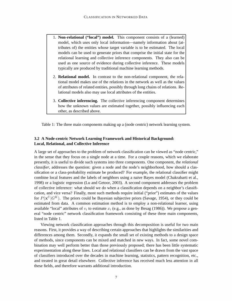
1. Non-relational (“local”) model. This component consists of a (learned)model, which uses only local information—namely information about (at-tributes of) the entities whose target variable is to be estimated. The localmodels can be used to generate priors that comprise the initial state for therelational learning and collective inference components.They also can beused as one source of evidence during collective inference.These modelstypically are produced by traditional machine learning methods.
2. Relational model. In contrast to the non-relational component, the rela-tional model makes use of the relations in the network as wellas the valuesof attributes of related entities, possibly through long chains of relations. Re-lational models also may use local attributes of the entities.
3. Collective inferencing. The collective inferencing component determineshow the unknown values are estimated together, possibly influencing eachother, as described above.
Table 1: The three main components making up a (node centric)network learning system.
3.2 A Node-centric Network Learning Framework and Historical Background:Local, Relational, and Collective Inference
A large set of approaches to the problem of network classification can be viewed as “node centric,”in the sense that they focus on a single node at a time. For a couple reasons, which we elaboratepresently, it is useful to divide such systems into three components. One component, therelationalclassifier, addresses the question: given a node and the node’s neighborhood, how should a clas-sification or a class-probability estimate be produced? Forexample, the relational classifier mightcombine local features and the labels of neighbors using a naive Bayes model (Chakrabarti et al.,1998) or a logistic regression (Lu and Getoor, 2003). A second component addresses the problemof collective inference: what should we do when a classification depends on a neighbor’s classifi-cation, and vice versa? Finally, most such methods require initial (“prior”) estimates of the valuesfor P (xU |GK). The priors could be Bayesian subjective priors (Savage, 1954), or they could beestimated from data. A common estimation method is to employa non-relational learner, usingavailable “local” attributes ofvi to estimatexi (e.g., as done by Besag (1986)). We propose a gen-eral “node centric” network classification framework consisting of these three main components,listed in Table 1.
Viewing network classification approaches through this decomposition is useful for two mainreasons. First, it provides a way of describing certain approaches that highlights the similarities anddifferences among them. Secondly, it expands the small set of existing methods to a design spaceof methods, since components can be mixed and matched in new ways. In fact, some novel com-bination may well perform better than those previously proposed; there has been little systematicexperimentation along these lines. Local and relational classifiers can be drawn from the vast spaceof classifiers introduced over the decades in machine learning, statistics, pattern recognition, etc.,and treated in great detail elsewhere. Collective inference has received much less attention in allthese fields, and therefore warrants additional introduction.
7
MACSKASSY AND PROVOST
Collective inference has its roots mainly in pattern recognition and statistical physics. Markovrandom fields have been used extensively for univariate network classification for vision and imagerestoration. Introductions to MRFs fill textbooks (Winkler, 2003); for our purposes, it is importantto point out that they are the basis both directly and indirectly for many network classification ap-proaches. MRFs are used to estimate the joint probability ofa set of nodes based on their immediateneighborhoods under the first-order Markov assumption thatP (xi|G/vi) = P (xi|Ni), wherexi isthe (estimated) label of vertexvi, G/vi means all nodes inG exceptvi, andNi is a neighborhoodfunction returning the neighbors ofvi. In a typical image application, nodes in the network arepixels and the labels are image properties such as whether a pixel is part of a vertical or horizontalborder.
Because of the obvious interdependencies among the nodes inan MRF, computing the jointprobability of assignments of labels to the nodes (“configurations”) requires collective inference.Gibbs sampling (Geman and Geman, 1984) was developed for this purpose for restoring degradedimages. Geman and Geman enforce that the Gibbs sampler settles to a final state by using simu-lated annealing where the temperature is dropped slowly until nodes no longer change state. Gibbssampling is discussed in more detail below.
Besag (1986) notes two problems with Gibbs sampling that areparticularly relevant for machinelearning applications of network classification. First, prior to this paper Gibbs sampling typicallywas used in vision not to compute the final marginal posteriors, as required by many “scoring”applications where the goal is to rank individuals, but rather to get final MAP classifications. Sec-ond, Gibbs sampling can be very time consuming, especially for large networks (not to mentionthe problems detecting convergence in the first place). Withhis Iterated Conditional Modes (ICM)algorithm, Besag introduced the notion ofiterative classificationfor scene reconstruction. In brief,iterative classification repeatedly classifies labels forvi ∈ V
U , based on the “current” state of thegraph, until no vertices change their label. ICM is presented as being efficient and particularly wellsuited to maximum marginal classification by node (pixel), as opposed to maximum joint classifi-cation over all the nodes (the scene).
Two other, closely related, collective inference techniques are (loopy) belief propagation (Pearl,1988) and relaxation labeling (RL) (Rosenfeld et al., 1976;Hummel and Zucker, 1983). Loopybelief propagation was introduced above. Relaxation labeling originally was proposed as a classof parallel iterative numerical procedures that use contextual constraints to reduce ambiguities inimage analysis; an instance of relaxation labeling is described in detail below. Both methods usethe estimated class distributions directly, rather than the hard labelings used by iterative classifica-tion. Therefore, one requirement for applying these methods is that the relational classifier, whenestimatingxi, must be able to use the estimated class distributions ofvj ∈ NU
i .
Graph-cut techniques recently have been used in vision research as an alternative to using Gibbssampling (Boykov et al., 2001). In essence, these are collective inference procedures, and are thebasis of a collection of modern machine learning techniques. However, they do not quite fit in thenode-centric framework, so we treat them separately below.
3.3 Node-centric Network Classification Approaches
The node-centric framework allows us to describe several prior systems by how they solve theproblems of local classification, relational classification, and collective inference. The componentsof these systems are the basis for composing methods in NetKit.
8
CLASSIFICATION IN NETWORKED DATA
Chakrabarti et al. (1998) studied classifying web-pages based on the text and (possibly inferred)class labels of neighboring pages. Their system pairs naiveBayes local and relational classifiers,with relaxation labeling for collective inference. In their experiments, performing network clas-sification using the web-pages’ link structure substantially improved classification as compared tousing only the local (text) information. Specifically, considering the text of neighboring pages gen-erally hurt performance, whereas using only the (inferred)class labels improved performance.
The ICM of Besag (1986) is a node-centric approach where the local and relational classifiersare domain-dependent probabilistic models (based on localattributes and a MRF), and iterative clas-sification is used for collective inference. Neville and Jensen (2000) applied naive Bayes classifiers,and used a simulated annealing approach in their iterative classification procedure, where on eachiteration a label for a given node is kept only if the relational classifier is confident in label at agiven threshold, otherwise the label is set tonull . By slowly lowering this threshold, the systemeventually labels all nodes.
Also applying iterative classification for collective inference, Lu and Getoor (2003) investigatednetwork classification of linked documents (web pages and published manuscripts with an accom-panying citation graph). Similarly to the work of Chakrabarti et al. (1998), Lu and Getoor (2003)used the (local) text of the document as well as neighbor labels. More specifically, their “link-based”relational classifier is a logistic regression model applied to a vector of aggregations of propertiesof the sets of neighbor labels linked with different types oflinks (in-, out-, co-links). They considervarious aggregates, such as the mode (the value of the most often occurring neighbor class), a binaryvector with a value of 1 at celli if there was a neighbor whose class label wasci, and a count vectorwhere celli contained the number of neighbors belonging to classci. In their experiments, the countmodel performed best. They used logistic regression on the local (text) attributes of the instances toinitialize the priors for each vertex in their graph and thenapplied the link-based classifiers as theirrelational model.
Macskassy and Provost (2003) investigated a simple univariate classifier, the weighted-vote re-lational neighbor (wvRN). They instantiated node priors simply by the marginal class frequencyin the training data. wvRN performs relational classification via a weighted average of the esti-mated class membership scores (“probabilities”) of the node’s neighbors. Collective inference isperformed via a relaxation labeling method similar to that used by Chakrabarti et al. (1998).
Since wvRN performs so well in the case study, it is noteworthy to point out its close rela-tionship to Hopfield networks (Hopfield, 1982) and Boltzmannmachines (Hinton and Sejnowski,1986). A Hopfield network is a graph of homogeneous nodes and undirected edges, where eachnode is a binary threshold unit. Hopfield networks were designed to recover previously seen graphconfigurations from a partially observed configuration, by repeatedly estimating the states of nodesone at a time. The state of a node is determined by whether or not its input exceeds its threshold,where the input is the weighted sum of the states of its immediate neighbors. wvRN differs in thatit retains uncertainty at the nodes rather than assigning each a binary states (also allowing multi-class networks).Learning in Hopfield networks consists of learning the weights of edges and thethresholds of nodes, given one or more input graphs. Given a partially observed graph state andrepeatedly applying, node-by-node, the node-activation equation will provably converge to a stablegraph state—the low-energy state of the graph. If the partial input state is “close” to one of thetraining states, the Hopfield network will converge to that state.
A Boltzmann machine, like a Hopfield network, is a network of units with an “energy” definedfor the network (Hinton and Sejnowski, 1986). Unlike Hopfield networks, Boltzmann machine
9
MACSKASSY AND PROVOST
nodes are stochastic and the machines use simulated annealing to find a stable state. Boltzmannmachines also often have both visible and hidden nodes. The visible nodes’ states can be observed,whereas the states of the hidden nodes cannot—much like hidden Markov models (HMMs). As withHMMs, the complete state of a Boltzmann machine often is found using algorithms like expectationmaximization, where thresholds and weights are computed inthe maximization step and the states ofthe nodes are determined in the estimation step. One challenge for Boltzmann machines is that theyare expensive computationally and therefore difficult or impossible to apply to large-scale networks.
3.4 Other Methods for Network Classification
Before describing the node-centric network classificationtoolkit, for completeness we first willdiscuss three other types of methods that are suited to within-network classification. Graph-basedmethods have been introduced for semi-supervised learning, and could apply as well to within-network classification. Within-network classification also offers the opportunity to take advantageof node identifiers, discussed in Section 3.4.2. Finally, although there are important reasons to studyunivariate network classification (see below), recently the field has seen a flurry of development ofmultivariate methods applicable to classification in networked data (Section 3.4.3).
3.4.1 GRAPH-CUT METHODS AND THERELATIONSHIP TO TRANSDUCTIVE INFERENCE
As mentioned above, one complication to within-network classification is that in the same networkthe to-be-classified nodes are intermixed with nodes for which the labels are known. Most priorwork on network learning and classification assumes that theclasses of all the nodes in the networkneed to be estimated (perhaps having learned something froma separate, related network). Pinningthe values of certain nodes intuitively should be advantageous, since it gives to the classificationprocedure clear points of reference.
This complication is addressed directly by several lines ofrecent work (by Blum and Chawla(2001), by Joachims (2003), by Zhu et al. (2003), and by Blum et al. (2004)). In this work, the set-ting is not initially one of network classification. Rather,these techniques are designed to addresssemi-supervised learning in a transductive setting (Vapnik, 1998b), but their methods may have di-rect application to certain instances of univariate network classification. Specifically, they considerdata sets where labels are given for a subset of cases, and classifications are desired for a subset ofthe rest. They connect the data into a weighted network, by adding edges (in various ways) basedon similarity between cases.
In the computer vision literature, Greig et al. (1989) pointout that finding the minimum energyconfiguration of a MRF, the partition of the nodes that maximizes self-consistency under the con-straint that the configuration be consistent with the known labels, is equivalent to finding a minimumcut of the graph. Blum and Chawla (2001) follow this idea and subsequent work by Kleinberg andTardos (1999) connecting the classification problem to the problem of computing minimum cuts.They investigate how to define weighted edges for a transductive classification problem such thatpolynomial-time mincut algorithms give optimal solutionsto objective functions of interest. Forexample, they show elegantly how forms of leave-one-out-cross-validation error (on the predictedlabels) can be minimized for various nearest-neighbor algorithms, including a weighted-voting al-gorithm. This procedure corresponds to optimizing the consistency of the predictions in particularways—as Blum and Chawla put it, optimizing the “happiness” of the classification algorithm. Ofcourse, optimizing the consistency of the labeling may not be ideal, for example in the case of highly
10
CLASSIFICATION IN NETWORKED DATA
unbalanced class frequency. Joachims (2003) points out that the need to preprocess the graph toavoid degenerate cuts (e.g, cutting off the one positive example) stems from the basic objective: theminimum of the sum of cut-through edge weights depends directly on the sizes of the cut sets. Heproposes to normalize for the cut size, and introduces a solution based on ratiocut optimization con-strained by the known labels, following the unconstrained procedure proposed by Dhillon (2001)for unsupervised learning.
Subsequently, Blum et al. (2004) point out that the min-cut solution corresponds to the mostprobable joint labeling of the graph (taking an MRF perspective), whereas as discussed earlier weoften would like a per-node (marginal) class-probability estimation. Unfortunately, in the case weare considering—when some node labels are known in a generalgraph—there is no known algo-rithm for determining these estimates. They also point out several other drawbacks, including thatthere may be many minimum cuts for a graph (from which mincut algorithms choose rather arbi-trarily), and that the min-cut approach does not yield a measure of confidence on the classifications.Blum et al. address these drawbacks by repeatedly adding artificial noise to the edge weights inthe induced graph. They then can compute fractional labels for each node corresponding to thefrequency of labeling by the various min-cut instances. As mentioned above, this method (and thefollowing) was intended to be applied to an induced graph, which can be designed specifically forthe application. Blum et al. point out that min-cut approaches are appropriate for graphs that haveat least some small, balanced cuts (whether or not these correspond to the labeled data), and fur-thermore their method discards highly unbalanced cuts. So,it is not clear whether it would apply tonetwork classification problems such as fraud detection in transaction networks.
In the experiments of Blum et al. (2004), their randomized min-cut method empirically doesnot perform as well as the method introduced by Zhu et al. (2003). Therefore, we will revisit themethod of Zhu et al. in an experimental comparison below, following the main case study. Inthe same transductive setting as Blum et al., Zhu et al. treatthe induced network as a Gaussianfield (a random field with soft node labels) constrained such that the labeled nodes maintain theirvalues. The value of the energy function is the weighted average of the function’s values at theneighboring points. Zhu et al. show that this function is a harmonic function and that the solutionover the complete graph can be computed using a few matrix operations. The result is a classifieressentially identical to the wvRN classifier discussed above (paired with relaxation labeling), exceptwith a principled semantics and exact inference.3 The energy function then can be normalizedbased on desired class priors (“class mass normalization”). Zhu et al. also discuss various physicalinterpretations of this procedure, including random walks, electric networks, and spectral graphtheory, that can be intriguing in the context of particular applications. For example, applying therandom walk interpretation to a telecommunications network including legitimate and fraudulentaccounts, consider starting at an account of interest and walking randomly through the call graphbased on the link weights; the node score is the probability that the walk hits a known fraudulentaccount before hitting a known legitimate account.
3.4.2 USING NODE IDENTIFIERS
As mentioned in the introduction, another unique aspect of within-network classification is thatnodeidentifiers, unique symbols for individual nodes, can be used in learning and inference. For example,
3. Experiments show these two procedures to yield almost identical generalization performance, albeit the matrix-basedprocedure of Zhu et al. is much slower than the iterative wvRN.
11
MACSKASSY AND PROVOST
for suspicion scoring in social networks, the fact that someone met with a particular individual maybe informative (e.g., having had repeated meetings with a known terrorist leader). Very little workhas incorporated identifiers, because of the obvious difficulty of modeling with very high cardinalitycategorical attributes. Fawcett and Provost (1997) and Cortes et al. (2001) describe the use ofidentifiers (telephone numbers) for fraud detection. To ourknowledge, Perlich and Provost (2006)provide the only comprehensive treatment of this topic, a topic which could benefit from furtherresearch.
3.4.3 BEYOND UNIVARIATE CLASSIFICATION
Besides the methods already discussed (e.g., (Besag, 1986;Lu and Getoor, 2003; Chakrabarti et al.,1998)), several other methods go beyond the homogeneous, univariate case on which this paperfocuses. Conditional Random Fields (CRFs) (Lafferty et al., 2001) are random fields where theprobability of a node’s label is conditioned not only on the labels of neighbors (as in MRFs), butalso on the entire observed attribute dataX.
Relational Bayesian Networks (RBNs, a.k.a. ProbabilisticRelational Models) (Koller and Pfef-fer, 1998; Friedman et al., 1999; Taskar et al., 2001) extendBayesian networks (BNs (Pearl, 1988))by taking advantage of the fact that a variable used in one instantiation of a BN may refer to the exactsame variable in another BN. For example, if the grade of a student depends upon his professor, thisprofessor is the same for all students in the class. Therefore, rather than building one BN and usingit in isolation for each entity, RBNs directly link shared variables, thereby generating one big net-work of connected entities for which collective inferencing can be performed. For within-networkclassification RBNs were applied by Taskar et al. (2001) to various domains, including a data setof published manuscripts linked by authors and citations. Loopy belief propagation (Pearl, 1988)was used to perform the collective inferencing. The study showed that the PRM performed betterthan a non-relational naive Bayes classifier and that using both author and citation information inconjunction with the text of the paper worked better than using only author or citation informationin conjunction with the text. We revisit this study below.
Relational Dependency Networks (RDNs) (Neville and Jensen, 2003, 2004), extend depen-dency networks (Heckerman et al., 2000) in much the same way that RBNs extend Bayes Net-works. (Gibbs sampling was used for collective inference.)Similarly, Relational Markov Networks(RMNs) (Taskar et al., 2002) extend Markov Networks (Pearl,1988). The clique potential func-tions are based on functional templates, each of which is a (learned, class-conditional) probabilityfunction based on a user-specified set of relations. Taskar et al. (2002) applied RMNs to a set ofweb-pages and showed that they performed better than other non-relational learners as well as naiveBayes and logistic regression when used with the same relations as the RMN. (Loopy belief prop-agation was used for collective inference.) Associative Markov Networks (AMNs) (Taskar et al.,2004) is another extension of the Markov Network, where auto-correlation of labels is explicitlytaken into account. AMNs extend thegeneralized Potts model(Potts, 1952) to allow different labelsto have different penalties. Exact inferencing in AMNs is formulated as a quadratic programmingproblem for binary classification and can be relaxed for multi-class problems.
Neville and Jensen (2005) proposed using latent group models (LGMs) to specify joint modelsof attributes, links, andgroups. Shared membership in groups such as communities with sharedinterests is an important reason for similarity among interconnected nodes, such as the ubiquitoushomophily we see in the case study. Inference can be more effective if these groups are modeled
12

CLASSIFICATION IN NETWORKED DATA
Input: GK , V U , RCtype, LCtype, CItype
Induce a local classification model, LC, of type LCtype, usingGK
Induce a relational classification model, RC, of type RCtype, usingGK
Estimatexi ∈ V U using LC.Apply collective inferencing of type CItype, using RC as the model.Output: Final estimates forxi ∈ V U
Table 2: High-level pseudo code for the core routine of the Network Learning Toolkit.
explicitly, as Neville and Jensen show. LGMs are especiallypromising for within-network clas-sification, since the existence of known classes will facilitate the identification of (hidden) groupmembership, which in turn may aid in the estimation ofx
U .These methods for network classification use only a few of themany relational learning tech-
niques. There are many more, for example from the rich literature of inductive logic programming(ILP) (e.g. (Flach and Lachiche, 1999; De Raedt et al., 2001; Dzeroski and Lavrac, 2001; Krameret al., 2001; Richardson and Domingos, 2006)), or based on using relational database joins to gen-erate relational features (e.g. (Perlich and Provost, 2003; Popescul and Ungar, 2003; Perlich andProvost, 2006)).
4. Network Learning Toolkit (NetKit-SRL)
NetKit is designed to accommodate the interchange of node-centric components and the introduc-tion of new components. As outlined in Section 3.2, the node-centric learning framework comprisesthree main components: the relational classifier, the localclassifier and collective inferencing. Anylocal classifier can be paired with any relational classifier, which can then be combined with anycollective inference method. NetKit’s core routine is simple and is outlined in Table 2.
NetKit consists of these five general modules:
1. Input: This module reads data into a memory-resident graphG.
2. Local classifier inducer (LC): Given as training dataV K , this module returns a model thatwill estimatexi using only attributes of a nodevi ∈ V U . Ideally, LC will estimate a proba-bility distribution over the possible values forxi.
3. Relational classifier inducer (RC): GivenGK , this module returns a modelMR that willestimatexi usingvi andNi. Ideally,MR will estimate a probability distribution over thepossible values forxi.
4. Collective Inferencing (CI): Given a graphG possibly with somexi known, a set of priorsoverxU , and a relational modelMR, this module applies collective inferencing to estimatex
U .
5. Weka Wrapper: This module is a wrapper for Weka4 (Witten and Frank, 2000) and willconvert the graph representation ofvi into an entity that can either be learned from or be used
4. We use version 3.4.2. Weka is available athttp://www.cs.waikato.ac.nz/˜ml/weka/
13
MACSKASSY AND PROVOST
to estimatexi. NetKit can use a Weka classifier both as a local classifier as well as a relationalclassifier (by using various aggregation methods to summarize the values of attributes inNi).
The current version of NetKit-SRL, while able to read in heterogeneous graphs, only supportsclassification in graphs consisting of a single type of node.Algorithms based on expectation maxi-mization are possible to implement through the NetKit CI module, by having the CI module repeat-edly apply RC to learn a new relational model and then apply the new relational model onG (ratherthan repeatedly apply the same learned model at every iteration).
The rest of this section describes the particular relational classifiers and collective inferencemethods implemented in NetKit for the case study. First, we describe the four (univariate5) rela-tional classifiers (RC components). Then, we describe the three collective inference (CI) methods.
4.1 Relational Classifiers (RC)
All four relational classifiers take advantage of the first-order Markov assumption on the network:only a node’s local neighborhood is necessary for classification. The univariate case renders thisassumption particularly restrictive: only the class labels of the local neighbors are necessary. Thelocal network is defined by the user, analogous to the user’s definition of the feature set for proposi-tional learning. Entities whose class labels are not known are either ignored or are assigned a priorprobability, depending upon the choice of local classifier.
4.1.1 WEIGHTED-VOTE RELATIONAL NEIGHBOR CLASSIFIER (WVRN)
Our first and simplest classifier (cf., Macskassy and Provost(2003)6) estimates class-membershipprobabilities based on one assumption in addition to the Markov assumption: the entities exhibithomophily—i.e., linked entities have a propensity to belong to the same class (Blau, 1977; McPher-son et al., 2001). This homophily-based model is motivated by observations and theories of socialnetworks (Blau, 1977; McPherson et al., 2001), where homophily is ubiquitous. Homophily wasone of the first characteristics noted by early social network researchers (Almack, 1922; Bott, 1928;Richardson, 1940; Loomis, 1946; Lazarsfeld and Merton, 1954), and holds for a wide variety ofdifferent relationships (McPherson et al., 2001). It seemsreasonable to conjecture that homophilymay also be present in other sorts of networks, especially networks of artifacts created by people.(Recentlyassortativity, a link-centric notion of homophily, has become the focus ofmathematicalstudies of network structure (Newman, 2003).)
Definition. Givenvi ∈ V U , the weighted-vote relational-neighbor classifier (wvRN)estimatesP (xi|Ni) as the (weighted) mean of the class-membership probabilities of the entities inNi:
P (xi = X|Ni) =1
Z
∑
vj∈Ni
wi,j · P (xj = X|Nj), (2)
whereZ is the usual normalizer. As this is a recursive definition (for undirected graphs,vj ∈ Ni ⇔vi ∈ Nj) the classifier uses the “current” estimate forP (xj = X |Nj), where the current estimate isdefined by the collective inference technique being used.
5. The open-source NetKit release contains multivariate versions of these classifiers.6. Previously called the probabilistic Relational Neighbor classifier (pRN).
14
CLASSIFICATION IN NETWORKED DATA
4.1.2 CLASS-DISTRIBUTION RELATIONAL NEIGHBOR CLASSIFIER (CDRN)
Learninga model of the distribution of neighbor class labels may leadto better discrimination thansimply using the (weighted) mode. Following Perlich and Provost (2003, 2006), and in the spiritof Rocchio’s method (Rocchio, 1971), we define nodevi’s class vectorCV(vi) to be the vector ofsummed linkage weights to the various (known) classes, and classX ’s reference vectorRV(X) tobe the average of the class vectors for nodes known to be of classX. Specifically:
CV(vi)k =∑
vj∈Ni,xj=Xk
wi,j , (3)
whereCV(vi)k represents thekth position in the class vector andXk is thekth class. Based onthese class vectors, the reference vectors can then be defined as the normalized vector sum:
RV(X) =1
|V KX |
∑
vi∈V KX
CV(vi), (4)
whereV KX = {vi|vi ∈ V K , xi = X}.
During training, neighbors inV U are ignored. For prediction, estimated class membershipprobabilities are used for neighbors inV U , and equation (3) becomes:
CV(vi)k =∑
vj∈Ni
wi,j · P (xj = Xk|Nj) (5)
Definition. Given vi ∈ V U , the class-distribution relational-neighbor classifier (cdRN) es-timates the probability of class membership,P (xi = X |Ni), by the normalized vector distancebetweenvi’s class vector and classX ’s reference vector:
P (xi = X|Ni) =1
Zdist(CV(vi),RV(X)), (6)
whereZ is the usual normalizer anddist(a, b) is any vector distance function (L1, L2, cosine, etc.).For the results presented below, we use cosine distance.
As with wvRN, Equation 5 is a recursive definition, and therefore the value ofP (xj = X|Nj)is approximated by the “current” estimate as given by the selected collective inference technique.
4.1.3 NETWORK-ONLY BAYES CLASSIFIER (NBC)
NetKit’s network-only Bayes classifier (nBC) is based on thealgorithm described by Chakrabartiet al. (1998). To start, assume there is a single nodevi in V U . The nBC uses multinomial naiveBayesian classification based on the classes ofvi’s neighbors.
P (xi = X|Ni) =P (Ni|X) · P (X)
P (Ni), (7)
where
P (Ni|X) =1
Z
∏
vj∈Ni
P (xj = Xj∗ |xi = X)wi,j (8)
15
MACSKASSY AND PROVOST
whereZ is a normalizing constant andXj∗ is the class observed at nodevj . As usual, becauseP (Ni) is the same for all classes, normalization across the classes allows us to avoid explicitlycomputing it.
We call nBC “network-only” to emphasize that in the application to the univariate case studybelow, we do not use local attributes of a node. As discussed above, Chakrabarti et al. initializenodes’ priors based on a naive Bayes model over the local document text and add a text-basedterm to the node probability formula.7 In the univariate setting, local text is not available. Wetherefore use the same scheme as for the other RCs: initialize unknown labels as decided by thelocal classifier being used (in our study: either the class prior or ’null ’, depending on the CIcomponent, as described below). If a neighbor’s label is ’null ’, then it is ignored for classification.Also, Chakrabarti et al. differentiated between incoming and outgoing links, whereas we do not.Finally, Chakrabarti et al. do not mention how or whether they account for possible zeros in theestimations of the marginal conditional probabilities; weapply traditional Laplace smoothing wherem = |X |, the number of classes.
The foregoing assumes all neighbor labels are known. When the values of some neighbors areunknown, but estimations are available, we follow Chakrabarti et al. (1998) and perform Markovrandom field estimations (Dobrushin, 1968; Geman and Geman,1984; Winkler, 2003), based onhow different configurations of neighbors’ classes affect atarget entity’s class. Specifically, theclassifier computes a Bayesian combination based on (estimated) configuration priors and the en-tity’s known neighbors. Chakrabarti et al. (1998) describethis procedure in detail. For our casestudy, such an estimation is necessary only when using relaxation labeling (described below).
4.1.4 NETWORK-ONLY L INK -BASED CLASSIFICATION (NLB)
The final relational classifier used in the case study is a network-only derivative of the link-basedclassifier (Lu and Getoor, 2003). The network-only Link-Based classifier (nLB) creates a featurevector for a node by aggregating the labels of neighboring nodes, and then uses logistic regressionto build a discriminative model based on these feature vectors. This learned model is then appliedto estimateP (xi = X |Ni). As with the nBC, the difference between the “network-only”link-basedclassifier and Lu and Getoor’s version is that for the univariate case study we do not consider localattributes (e.g., text).
As described above, Lu and Getoor (2003) considered variousaggregation methods: existence(binary), the mode, and value counts. The last aggregation method, the count model, is equivalentto the class vectorCV(vi) defined in Equation 5. This was the best performing method in the studyby Lu and Getoor, and is the method on which we base nLB. The logistic regression classifier usedby nLB is the multiclass implementation from Weka version 3.4.2.
We made one minor modification to the original link-based classifier. Perlich (2003) argues thatin different situations it may be preferable to use either vectors based on raw counts (as given above)or vectors based on normalized counts. We did preliminary runs using both. The normalized vectorsgenerally performed better, and so we use them for the case study.
7. The original classifier was defined as:P (xi = X |Ni) = P (Ni|X) · P (τi|vi) · P (X), with τi being the text of thedocument-entity represented by vertexvi.
16

CLASSIFICATION IN NETWORKED DATA
1. Initializevi ∈ V U using the local classifier model,ML. Specifically, forvi ∈ V U :
(a) ci ←ML(vi), whereci is a vector of probabilities (probability distribution)which representsML’s estimate ofP (xi|Ni).For the case study, the local classifier model returns the marginal class distri-bution estimated fromxK .
(b) Sample a valuexs from ci.
(c) Setxi ← xs.
2. Generate a random ordering,O, of vertices inV U .
3. For elementsvi ∈ O in order:
(a) Apply the relational classifier model:ci ←MR(vi).
(b) Sample a valuexs from ci.
(c) Setxi ← xs.Note that whenMR is applied toxi it uses the “new” labelings from elements1, . . . , (i−1), while using the “current” labelings for elements(i+1), . . . , n.
4. Repeat prior step200 times without keeping any statistics. This is known as theburnin period.
5. Repeat again for2000 iterations, counting the number of times eachxi is assigned aparticular valueX ∈ X . Normalizing these counts forms the final class probabilityestimates.
Table 3: Pseudo-code for Gibbs sampling.
4.2 Collective Inference Methods (CI)
This section describes three collective inferencing (CI) methods implemented in NetKit and usedin the case study. As described above, given (i) a network initialized by the local model, and (ii)a relational model, a CI method infers a set of class labels for x
U . Depending on the application,the goal ideally would be to infer the class labels with either the maximum joint probability orthe maximum marginal probability for each node. Alternatively, if estimates of entities’ class-membership probabilities are needed, the CI method estimates the marginal probability distributionP (xi|GK ,Λ) for eachxi ∈ x
U , whereΛ stands for the priors returned by the local classifier.
4.2.1 GIBBS SAMPLING (GS)
Gibbs sampling (GS) (Geman and Geman, 1984) is commonly usedfor collective inferencing withrelational learning systems. The algorithm is straightforward and is shown in Table 3.8 The use of200 and2000 for the burnin period and number of iterations are commonly used values.9 Ideally,we would iterate until the estimations converge. Although there are convergence tests for the Gibbs
8. This instance of Gibbs sampling uses a single random ordering (“chain”), as this is what we used in the case study.In the case study, using10 chains (the default in NetKit) had no effect on the final accuracies.
9. As it turns out, in our case study GS invariably reached a seemingly final plateau in fewer than1000 iterations, andoften in fewer than500.
17
MACSKASSY AND PROVOST
1. Forvi ∈ V U , initialize the prior: c(0)i ← ML(vi). For the case study, the local
classifier model returns the marginal class distribution estimated fromxK .
2. For elementsvi ∈ V U :
(a) Estimatexi by applying the relational model:
c(t+1)i ←MR(v
(t)i ), (9)
whereMR(v(t)i ) denotes using the estimatesc
(t)j for vj ∈ Ni, andt is the
iteration count. This has the effect that all predictions are done pseudo-simultaneously based on the state of the graph after iteration t.
3. Repeat forT iterations, whereT = 99 for the case study.c(T ) will comprise thefinal class probability estimations.
Table 4: Pseudo-code for Relaxation Labeling.
sampler, they are neither robust nor well understood (cf. Gilks et al. (1995)), so we simply use afixed number of iterations.
Notably, because all nodes are assigned a class at every iteration, when GS is used the relationalmodels will always see a fully labeled/classified neighborhood, making prediction straightforward.For example, nBC does not need its MRF estimation.
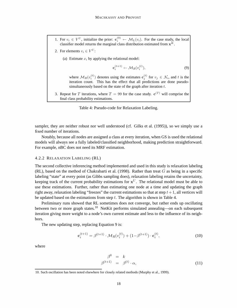
4.2.2 RELAXATION LABELING (RL)
The second collective inferencing method implemented and used in this study is relaxation labeling(RL), based on the method of Chakrabarti et al. (1998). Rather than treatG as being in a specificlabeling “state” at every point (as Gibbs sampling does), relaxation labeling retains the uncertainty,keeping track of the current probability estimations forx
U . The relational model must be able touse these estimations. Further, rather than estimating onenode at a time and updating the graphright away, relaxation labeling “freezes” the current estimations so that at stept+1, all vertices willbe updated based on the estimations from stept. The algorithm is shown in Table 4.
Preliminary runs showed that RL sometimes does not converge, but rather ends up oscillatingbetween two or more graph states.10 NetKit performs simulated annealing—on each subsequentiteration giving more weight to a node’s own current estimate and less to the influence of its neigh-bors.
The new updating step, replacing Equation 9 is:
c(t+1)i = β(t+1) ·MR(v
(t)i ) + (1−β(t+1)) · c
(t)i , (10)
where
β0 = k
β(t+1) = β(t) · α, (11)
10. Such oscillation has been noted elsewhere for closely related methods (Murphy et al., 1999).
18
CLASSIFICATION IN NETWORKED DATA
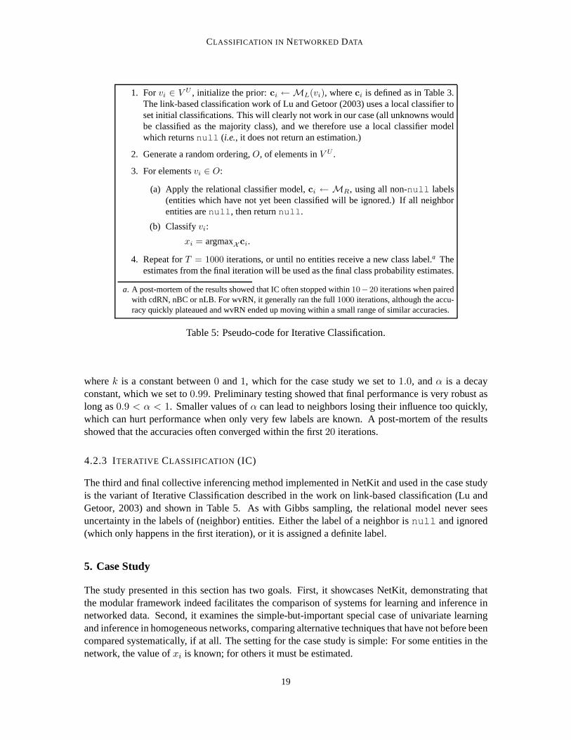
1. Forvi ∈ V U , initialize the prior:ci ←ML(vi), whereci is defined as in Table 3.The link-based classification work of Lu and Getoor (2003) uses a local classifier toset initial classifications. This will clearly not work in our case (all unknowns wouldbe classified as the majority class), and we therefore use a local classifier modelwhich returnsnull (i.e., it does not return an estimation.)
2. Generate a random ordering,O, of elements inV U .
3. For elementsvi ∈ O:
(a) Apply the relational classifier model,ci ← MR, using all non-null labels(entities which have not yet been classified will be ignored.) If all neighborentities arenull , then returnnull .
(b) Classifyvi:
xi = argmaxXci.
4. Repeat forT = 1000 iterations, or until no entities receive a new class label.a Theestimates from the final iteration will be used as the final class probability estimates.
a. A post-mortem of the results showed that IC often stopped within 10−20 iterations when pairedwith cdRN, nBC or nLB. For wvRN, it generally ran the full1000 iterations, although the accu-racy quickly plateaued and wvRN ended up moving within a small range of similar accuracies.
Table 5: Pseudo-code for Iterative Classification.
wherek is a constant between0 and1, which for the case study we set to1.0, andα is a decayconstant, which we set to0.99. Preliminary testing showed that final performance is very robust aslong as0.9 < α < 1. Smaller values ofα can lead to neighbors losing their influence too quickly,which can hurt performance when only very few labels are known. A post-mortem of the resultsshowed that the accuracies often converged within the first20 iterations.
4.2.3 ITERATIVE CLASSIFICATION (IC)
The third and final collective inferencing method implemented in NetKit and used in the case studyis the variant of Iterative Classification described in the work on link-based classification (Lu andGetoor, 2003) and shown in Table 5. As with Gibbs sampling, the relational model never seesuncertainty in the labels of (neighbor) entities. Either the label of a neighbor isnull and ignored(which only happens in the first iteration), or it is assigneda definite label.
5. Case Study
The study presented in this section has two goals. First, it showcases NetKit, demonstrating thatthe modular framework indeed facilitates the comparison ofsystems for learning and inference innetworked data. Second, it examines the simple-but-important special case of univariate learningand inference in homogeneous networks, comparing alternative techniques that have not before beencompared systematically, if at all. The setting for the casestudy is simple: For some entities in thenetwork, the value ofxi is known; for others it must be estimated.
19
MACSKASSY AND PROVOST
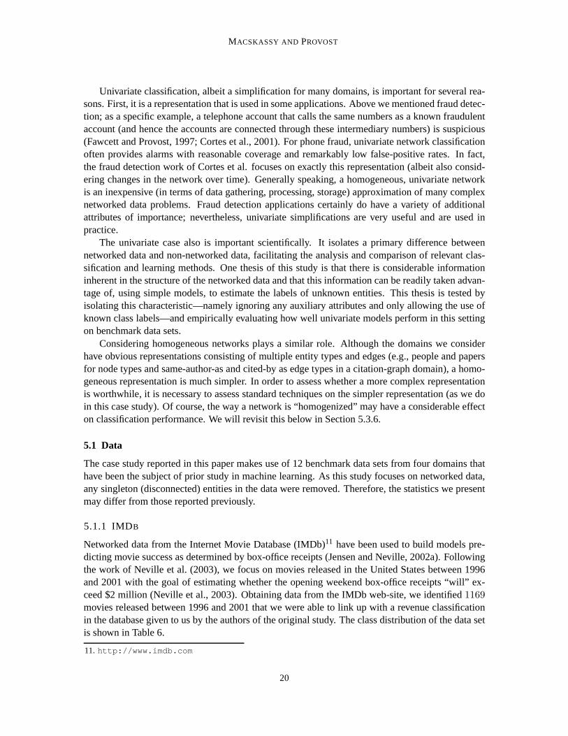
Univariate classification, albeit a simplification for manydomains, is important for several rea-sons. First, it is a representation that is used in some applications. Above we mentioned fraud detec-tion; as a specific example, a telephone account that calls the same numbers as a known fraudulentaccount (and hence the accounts are connected through theseintermediary numbers) is suspicious(Fawcett and Provost, 1997; Cortes et al., 2001). For phone fraud, univariate network classificationoften provides alarms with reasonable coverage and remarkably low false-positive rates. In fact,the fraud detection work of Cortes et al. focuses on exactly this representation (albeit also consid-ering changes in the network over time). Generally speaking, a homogeneous, univariate networkis an inexpensive (in terms of data gathering, processing, storage) approximation of many complexnetworked data problems. Fraud detection applications certainly do have a variety of additionalattributes of importance; nevertheless, univariate simplifications are very useful and are used inpractice.
The univariate case also is important scientifically. It isolates a primary difference betweennetworked data and non-networked data, facilitating the analysis and comparison of relevant clas-sification and learning methods. One thesis of this study is that there is considerable informationinherent in the structure of the networked data and that thisinformation can be readily taken advan-tage of, using simple models, to estimate the labels of unknown entities. This thesis is tested byisolating this characteristic—namely ignoring any auxiliary attributes and only allowing the use ofknown class labels—and empirically evaluating how well univariate models perform in this settingon benchmark data sets.
Considering homogeneous networks plays a similar role. Although the domains we considerhave obvious representations consisting of multiple entity types and edges (e.g., people and papersfor node types and same-author-as and cited-by as edge typesin a citation-graph domain), a homo-geneous representation is much simpler. In order to assess whether a more complex representationis worthwhile, it is necessary to assess standard techniques on the simpler representation (as we doin this case study). Of course, the way a network is “homogenized” may have a considerable effecton classification performance. We will revisit this below inSection 5.3.6.
5.1 Data
The case study reported in this paper makes use of 12 benchmark data sets from four domains thathave been the subject of prior study in machine learning. As this study focuses on networked data,any singleton (disconnected) entities in the data were removed. Therefore, the statistics we presentmay differ from those reported previously.
5.1.1 IMDB
Networked data from the Internet Movie Database (IMDb)11 have been used to build models pre-dicting movie success as determined by box-office receipts (Jensen and Neville, 2002a). Followingthe work of Neville et al. (2003), we focus on movies releasedin the United States between 1996and 2001 with the goal of estimating whether the opening weekend box-office receipts “will” ex-ceed $2 million (Neville et al., 2003). Obtaining data from the IMDb web-site, we identified1169movies released between 1996 and 2001 that we were able to link up with a revenue classificationin the database given to us by the authors of the original study. The class distribution of the data setis shown in Table 6.
11. http://www.imdb.com
20

CLASSIFICATION IN NETWORKED DATA
Category SizeHigh-revenue 572Low-revenue 597Total 1169Base accuracy 51.07%
Table 6: Class distribution for the IMDb data set.
Category SizeCase Based 402Genetic Algorithms 551Neural Networks 1064Probabilistic Methods 529Reinforcement Learning 335Rule Learning 230Theory 472Total 3583Base accuracy 29.70%
Table 7: Class distribution for the CoRA data set.
We link movies if they share a production company, based on observations from previous work12
(Macskassy and Provost, 2003). The weight of an edge in the resulting graph is the number ofproduction companies two movies have in common. Notably, weignore the temporal aspect of themovies in this study, simply labeling movies at random for the training set. This can lead to a moviein the test set being released earlier than a movie in the training set.
5.1.2 CORA
The CoRA data set (McCallum et al., 2000) comprises computerscience research papers. It includesthe full citation graph as well as labels for the topic of eachpaper (and potentially sub- and sub-sub-topics).13 Following a prior study (Taskar et al., 2001), we focused on papers within the machinelearning topic with the classification task of predicting a paper’s sub-topic (of which there are seven).The class distribution of the data set is shown in Table 7.
Papers can be linked in one of two ways: they share a common author, or one cites the other.Following prior work (Lu and Getoor, 2003), we link two papers if one cites the other. This numberordinarily would only be zero or one unless the two papers cite each other.
5.1.3 WEBKB
The third domain we draw from is based on the WebKB Project (Craven et al., 1998).14 It consists ofsets of web pages from four computer science departments, with each page manually labeled into7categories: course, department, faculty, project, staff,student or other. As with other work (Nevilleet al., 2003; Lu and Getoor, 2003), we ignore pages in the “other” category except as describedbelow.
12. And on a suggestion from David Jensen.13. These labels were assigned by a naive Bayes classifier (McCallum et al., 2000).14. We use the WebKB-ILP-98 data.
21

MACSKASSY AND PROVOST
Number of web-pagesClass Cornell Texas Washington Wisconsinstudent 145 163 151 155not-student 201 171 283 193Total 346 334 434 348Base accuracy 58.1% 51.2% 60.8% 55.5%
Table 8: Class distribution for the WebKB data set using binary class labels.
Number of web-pagesCategory cornell texas washington wisconsincourse 54 51 170 83department 25 36 20 37faculty 62 50 44 37project 54 28 39 25staff 6 6 10 11student 145 163 151 155Total 346 334 434 348Base accuracy 41.9% 48.8% 39.2% 44.5%
Table 9: Class distribution for the WebKB data set using six-class labels.
From the WebKB data we produce eight networked data sets for within-network classification.For each of the four universities, we consider two differentclassification problems: the six-classproblem, and following a prior study, the binary classification task of predicting whether a pagebelongs to a student (Neville et al., 2003).15 The binary task results in an approximately balancedclass distribution.
Following prior work on web-page classification, we link twopages by co-citations (ifx linksto z andy links to z, thenx andy are co-citingz) (Chakrabarti et al., 1998; Lu and Getoor, 2003).To weight the link betweenx andy, we sum the number of hyperlinks fromx to z and separatelythe number fromy to z, and multiply these two quantities. For example, if studentx has2 edgesto a group page, and a fellow studenty has3 edges to the same group page, then the weight alongthat path between those2 students would be6. This weight represents the number of possible co-citation paths between the pages. Co-citation relations are not uniquely useful to domains involvingdocuments; for example, as mentioned above, for phone-fraud detection bandits often call the samenumbers as previously identified bandits. We chose co-citations for this case study based on theprior observation that a student is more likely to have a hyperlink to her advisor or a group/projectpage rather than to one of her peers (Craven et al., 1998).16
To produce the final data sets, we extracted the pages that have at least one incoming and oneoutgoing link. We removed pages in the “other” category fromthe classification task, although theywere used as “background” knowledge—allowing2 pages to be linked by a path through an “other”
15. It turns out that the relative performance of the methodsis quite different on these two variants.16. We return to these data in Section 5.3.5, where we show anddiscuss how using the hyperlinks directly is not sufficient
for any of the univariate methods to do well.
22
CLASSIFICATION IN NETWORKED DATA
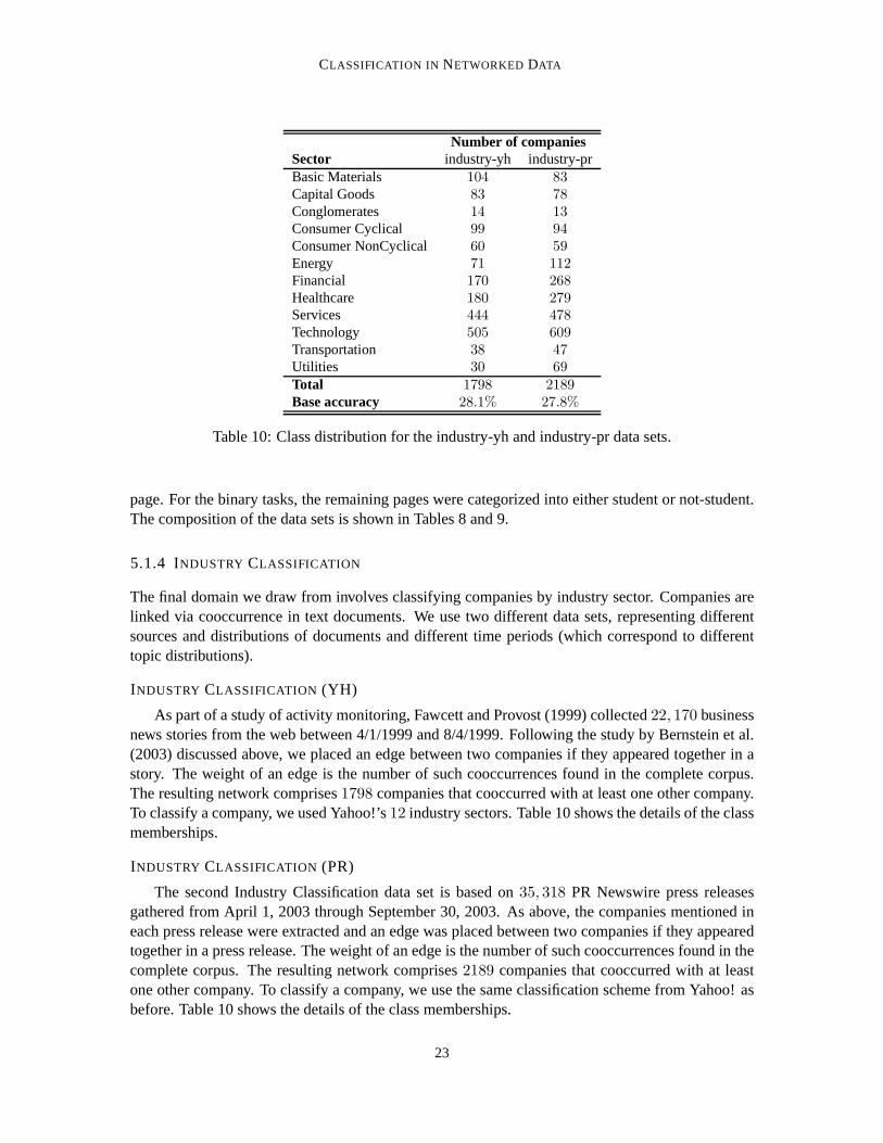
Number of companiesSector industry-yh industry-prBasic Materials 104 83Capital Goods 83 78Conglomerates 14 13Consumer Cyclical 99 94Consumer NonCyclical 60 59Energy 71 112Financial 170 268Healthcare 180 279Services 444 478Technology 505 609Transportation 38 47Utilities 30 69Total 1798 2189Base accuracy 28.1% 27.8%
Table 10: Class distribution for the industry-yh and industry-pr data sets.
page. For the binary tasks, the remaining pages were categorized into either student or not-student.The composition of the data sets is shown in Tables 8 and 9.
5.1.4 INDUSTRY CLASSIFICATION
The final domain we draw from involves classifying companiesby industry sector. Companies arelinked via cooccurrence in text documents. We use two different data sets, representing differentsources and distributions of documents and different time periods (which correspond to differenttopic distributions).
INDUSTRY CLASSIFICATION (YH)
As part of a study of activity monitoring, Fawcett and Provost (1999) collected22, 170 businessnews stories from the web between 4/1/1999 and 8/4/1999. Following the study by Bernstein et al.(2003) discussed above, we placed an edge between two companies if they appeared together in astory. The weight of an edge is the number of such cooccurrences found in the complete corpus.The resulting network comprises1798 companies that cooccurred with at least one other company.To classify a company, we used Yahoo!’s12 industry sectors. Table 10 shows the details of the classmemberships.
INDUSTRY CLASSIFICATION (PR)
The second Industry Classification data set is based on35, 318 PR Newswire press releasesgathered from April 1, 2003 through September 30, 2003. As above, the companies mentioned ineach press release were extracted and an edge was placed between two companies if they appearedtogether in a press release. The weight of an edge is the number of such cooccurrences found in thecomplete corpus. The resulting network comprises2189 companies that cooccurred with at leastone other company. To classify a company, we use the same classification scheme from Yahoo! asbefore. Table 10 shows the details of the class memberships.
23
MACSKASSY AND PROVOST
5.2 Experimental Methodology
NetKit allows for any combination of a local classifier (LC),a relational classifier (RC) and acollective inferencing method (CI). If we consider an LC-RC-CI configuration to be a completenetwork-classification method, we have12 to compare on each data set. Since, for this paper, theLC component is directly tied to the CI component (our LC components determine priors based onwhich CI component is being used), we henceforth consider annetwork-classification method to bean RC-CI configuration.
We first verify that the network structure alone (linkages plus known class labels) often con-tains a considerable amount of useful information for entity classification. We vary from10% to90% the percentage of nodes in the network for which class membership is known initially.17 Thestudy assesses: (1) whether the network structure enables accurate classification; (2) how muchprior information is needed in order to perform well, and (3)whether there are regular patterns ofimprovement across methods as the percentage of initially known labels increases.
Accuracy is averaged over10 runs. Specifically, given a data set,G = (V, E), the subset ofentities with known labelsV K (the “training” data set18) is created by selecting a class-stratifiedrandom sample of(100 × r)% of the entities inV . The test set,V U , is then defined asV−V K .We pruneV U by removing all nodes inzero-knowledgecomponents—nodes for which there is nopath to any node inV K . We use the same10 training/test partitions for each network-classificationmethod. Although it would be desirable to keep the test data disjoint (and therefore independent)as done in traditional machine learning via methods such as cross-validation, this is not applicablefor within-network learning. We keep the test node sets disjoint as much as possible between thedifferent runs. For example, atr = 0.90 (90% labeled data), our sets of testing nodes followstandard 10-fold cross-validation.
5.3 Results
5.3.1 INFORMATION IN THE NETWORK STRUCTURE
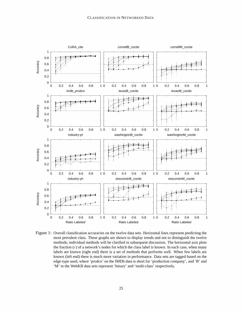
Figure 1 shows the accuracies of the12 network-classification methods across the12 data sets as thefraction (r) of entities for which class memberships are known increases fromr = 0.1 to r = 0.9.The purpose of these graphs is not to differentiate the curves, but to compare the general trends andthe levels of the accuracies to the baseline accuracies. In the univariate case, if the linkage structureis not known the only non-subjective alternative is to estimate using the class base rate (prior),which is shown by the horizontal line in the graphs. As is clear from Figure 1, all of the data setscontain considerable information in the class-linkage structure. The worst relative performance ison industry-pr, where at the right end of the curves the errorrate nonetheless is reduced by30–40%.The best performance is on webkb-texas, where the best methods reduce the error rate by close to90%. And in most cases, the better methods reduce the error rate by over50% toward the right endof the curves.
Machine learning studies on networked data sets seldom compare to simple network-classificationmethods like these, opting instead for comparing to non-relational classification. These results arguestrongly that comparisons also should be made to univariatenetwork classification, if the purpose
17. We also performed boundary experiments using the weighted-vote relational neighbor classifier with relaxation label-ing, where we decreased the number of initially known labelsdown to0.1% of the graph. The classification accuracygenerally degrades gracefully to doing no better than random guessing at this extreme.
18. These data will be used not only for training models, but also as existing background knowledge during classification.
24
CLASSIFICATION IN NETWORKED DATA
0
0.2
0.4
0.6
0.8
1
0 0.2 0.4 0.6 0.8 1
Acc
urac
y
CoRA_cite
0
0.2
0.4
0.6
0.8
1
0 0.2 0.4 0.6 0.8 1
cornellB_cocite
0
0.2
0.4
0.6
0.8
1
0 0.2 0.4 0.6 0.8 1
cornellM_cocite
0
0.2
0.4
0.6
0.8
1
0 0.2 0.4 0.6 0.8 1
Acc
urac
y
imdb_prodco
0
0.2
0.4
0.6
0.8
1
0 0.2 0.4 0.6 0.8 1
texasB_cocite
0
0.2
0.4
0.6
0.8
1
0 0.2 0.4 0.6 0.8 1
texasM_cocite
0
0.2
0.4
0.6
0.8
1
0 0.2 0.4 0.6 0.8 1
Acc
urac
y
industry-pr
0
0.2
0.4
0.6
0.8
1
0 0.2 0.4 0.6 0.8 1
washingtonB_cocite
0
0.2
0.4
0.6
0.8
1
0 0.2 0.4 0.6 0.8 1
washingtonM_cocite
0
0.2
0.4
0.6
0.8
1
0 0.2 0.4 0.6 0.8 1
Acc
urac
y
Ratio Labeled
industry-yh
0
0.2
0.4
0.6
0.8
1
0 0.2 0.4 0.6 0.8 1
Ratio Labeled
wisconsinB_cocite
0
0.2
0.4
0.6
0.8
1
0 0.2 0.4 0.6 0.8 1
Ratio Labeled
wisconsinM_cocite
Figure 1: Overall classification accuracies on the twelve data sets. Horizontal lines represent predicting themost prevalent class. These graphs are shown to display trends and not to distinguish the twelvemethods; individual methods will be clarified in subsequentdiscussion. The horizontal axis plotsthe fraction (r) of a network’s nodes for which the class label is known. In each case, when manylabels are known (right end) there is a set of methods that performs well. When few labels areknown (left end) there is much more variation in performance. Data sets are tagged based on theedge-type used, where ‘prodco’ on the IMDb data is short for ‘production company’, and ‘B’ and‘M’ in the WebKB data sets represent ‘binary’ and ‘multi-class’ respectively.
25
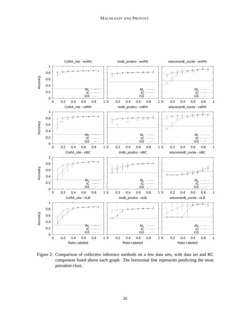
MACSKASSY AND PROVOST
0
0.2
0.4
0.6
0.8
1
0 0.2 0.4 0.6 0.8 1
Acc
urac
y
CoRA_cite - wvRN
RLIC
GS 0
0.2
0.4
0.6
0.8
1
0 0.2 0.4 0.6 0.8 1
imdb_prodco - wvRN
RLIC
GS 0
0.2
0.4
0.6
0.8
1
0 0.2 0.4 0.6 0.8 1
wisconsinB_cocite - wvRN
RLIC
GS
0
0.2
0.4
0.6
0.8
1
0 0.2 0.4 0.6 0.8 1
Acc
urac
y
CoRA_cite - cdRN
RLIC
GS 0
0.2
0.4
0.6
0.8
1
0 0.2 0.4 0.6 0.8 1
imdb_prodco - cdRN
RLIC
GS 0
0.2
0.4
0.6
0.8
1
0 0.2 0.4 0.6 0.8 1
wisconsinB_cocite - cdRN
RLIC
GS
0
0.2
0.4
0.6
0.8
1
0 0.2 0.4 0.6 0.8 1
Acc
urac
y
CoRA_cite - nBC
RLIC
GS 0
0.2
0.4
0.6
0.8
1
0 0.2 0.4 0.6 0.8 1
imdb_prodco - nBC
RLIC
GS 0
0.2
0.4
0.6
0.8
1
0 0.2 0.4 0.6 0.8 1
wisconsinB_cocite - nBC
RLIC
GS
0
0.2
0.4
0.6
0.8
1
0 0.2 0.4 0.6 0.8 1
Acc
urac
y
Ratio Labeled
CoRA_cite - nLB
RLIC
GS 0
0.2
0.4
0.6
0.8
1
0 0.2 0.4 0.6 0.8 1
Ratio Labeled
imdb_prodco - nLB
RLIC
GS 0
0.2
0.4
0.6
0.8
1
0 0.2 0.4 0.6 0.8 1
Ratio Labeled
wisconsinB_cocite - nLB
RLIC
GS
Figure 2: Comparison of collective inference methods on a few data sets, with data set and RCcomponent listed above each graph. The horizontal line represents predicting the mostprevalent class.
26

CLASSIFICATION IN NETWORKED DATA
sample ratio (r)0.10 0.20 0.30 0.40 0.50 0.60 0.70 0.80 0.90
RL v GS 0.002 0.001 0.001 0.001 0.002 0.001 0.001 0.010 0.010
RL v IC 0.025 0.100 0.100 0.025 0.002 0.002 0.001 0.005 0.002
IC v GS 0 .400 0.450 — 0.450 0 .400 — 0 .250 — 0.400
Table 11: p-values for the Wilcoxon Signed-Rank test, comparing the accuracies of pairs of CIcomponents across all data sets and RC methods. For each cell, bold text means that thefirst method was better than the second method and italics means it was worse. The cellswith ’—’ means there was no significant difference.
sample ratio (r)0.10 0.20 0.30 0.40 0.50 0.60 0.70 0.80 0.90 overall
RL 0.081 0.184 0.262 0.339 0.409 0.446 0.468 0.491 0.509 0.354
IC 0.000 0.116 0.235 0.314 0.382 0.423 0.452 0.482 0.503 0.323GS 0.029 0.126 0.231 0.301 0.385 0.421 0.450 0.474 0.502 0.324
Table 12: Relative error reductions (ERREL) for each CI component across all data sets. The lastcolumn, overall, is the average error reduction for each method across all sample ratios.Bold entries indicate the largest relative error reductionfor each sample ratio.
sample ratio (r)0.10 0.20 0.30 0.40 0.50 0.60 0.70 0.80 0.90 total
RL 11 11 10 7 4 5 6 4 6 64GS 1 1 0 1 5 3 4 4 4 23IC 0 0 2 4 3 4 2 4 2 21
Table 13: Number of times each CI method was the best across the12 data sets.
is to demonstrate the power of a more sophisticated relational learning method. We return to thisargument in Section 5.3.7.
5.3.2 COLLECTIVE INFERENCECOMPONENT
Figure 2 shows, for three of the data sets, the comparative performances of the three collectiveinference (CI) components. Each graph is for a particular relational classifier. The graphs show thatwhile the three CI components often perform similarly, their performances are clearly separated forlow values ofr.
Table 11 shows thep-values for a Wilcoxon Signed-Rank test assessing whether the first method(listed in column 1) is significantly better than the second.Specifically, for a given data set and labelratio (r), each network-classification experiment consists of10 random train/test splits—the samefor all configurations. For each pair of CI components, averaging the accuracies of the10 splitsacross the4 RC components gives one average accuracy score for each of the12 data sets yielding12 paired data points for each CI method. The results show clearly that RL, across the board,
27
MACSKASSY AND PROVOST
outperforms GS atp ≤ 0.01 and that RL is also better than IC across the board. Further, we see thatIC and GS are roughly comparable.
The foregoing gives some evidence that relaxation labelingis consistently better than iterativeclassification and Gibbs sampling when the results are pooled, especially at low values ofr.. Ta-ble 12 quantifies the differences. In order to be comparable across data sets with different base rates,the table shows the amount of error reduction over the base rate. As a simple example, assume thebase error rate is0.4, method A yields an error rate of0.1, and method B yields an error rate of0.2.Method A reduces the error by75%. Method B reduces the error by50%.
The relative error reduction of the CI components is defined as follows:
ERABS(RC,CI, D, r) = (baseerr(D)− err(RC-CI, D, r)) (12)
ERREL(RC,CI, D, r) =ERABS(RC,CI, D, r)
baseerr(D)(13)
ERREL(RC,CI, r) =1
|D|
∑
D∈D
ERREL(RC,CI, D, r) (14)
ERREL(CI, r) =1
|RC|
∑
RC∈RC
ERREL(RC,CI, r) (15)
(16)
where err(RC-CI,D, r) is the error for the configuration (RC and CI) on data setD with r% of thegraph being labeled.
Table 12 shows the relative error reductions for each CI component. RL outperformed IC acrossthe board, from as low as a1.3% improvement (r = 0.90) to as high as59% or better improvement(r ≤ 0.2) when averaged over all the data sets and RC methods. OverallRL improved performanceover IC by about10% as seen in the last column. Notably, RL’s advantage over IC improves mono-tonically as less is known in the network. Similar numbers and a similar pattern are seen for RLversus GS. IC and GS are comparable.
For another perspective, Table 13 shows, for each ratio as well as a total across all ratios, thenumber of times each CI implementation took part in the best-performing network-classificationcombination for each of the twelve data sets. Specifically, for each sampling ratio, each win for anRC-CI configuration counted as a win for the CI module of the pair (as well as a win for the RCmodule in the next section). For example, in Figure 2, the first column of four graphs shows theperformances of the 12 network-classification combinations on the CoRA data; at the left end of thecurves, wvRN-RL is the best performing combination. Table 13 adds further support to the conclu-sion that relaxation labeling (RL) was the overall best component, primarily due to its advantage atlow values ofr. We also see again that Gibbs Sampling (GS) and Iterative Classification (IC) werecomparable.
5.3.3 RELATIONAL MODEL COMPONENT
Comparing relational models, we would expect to see a certain pattern: if even moderate homophilyis present in the data, we would expect wvRN to perform well. Its nonexistent training variance19
should allow it to perform relatively well, even with small numbers of known labels in the net-work. The higher-variance nLB may perform relatively poorly with small numbers of known labels
19. There still will be variance due to the set of known labels.
28
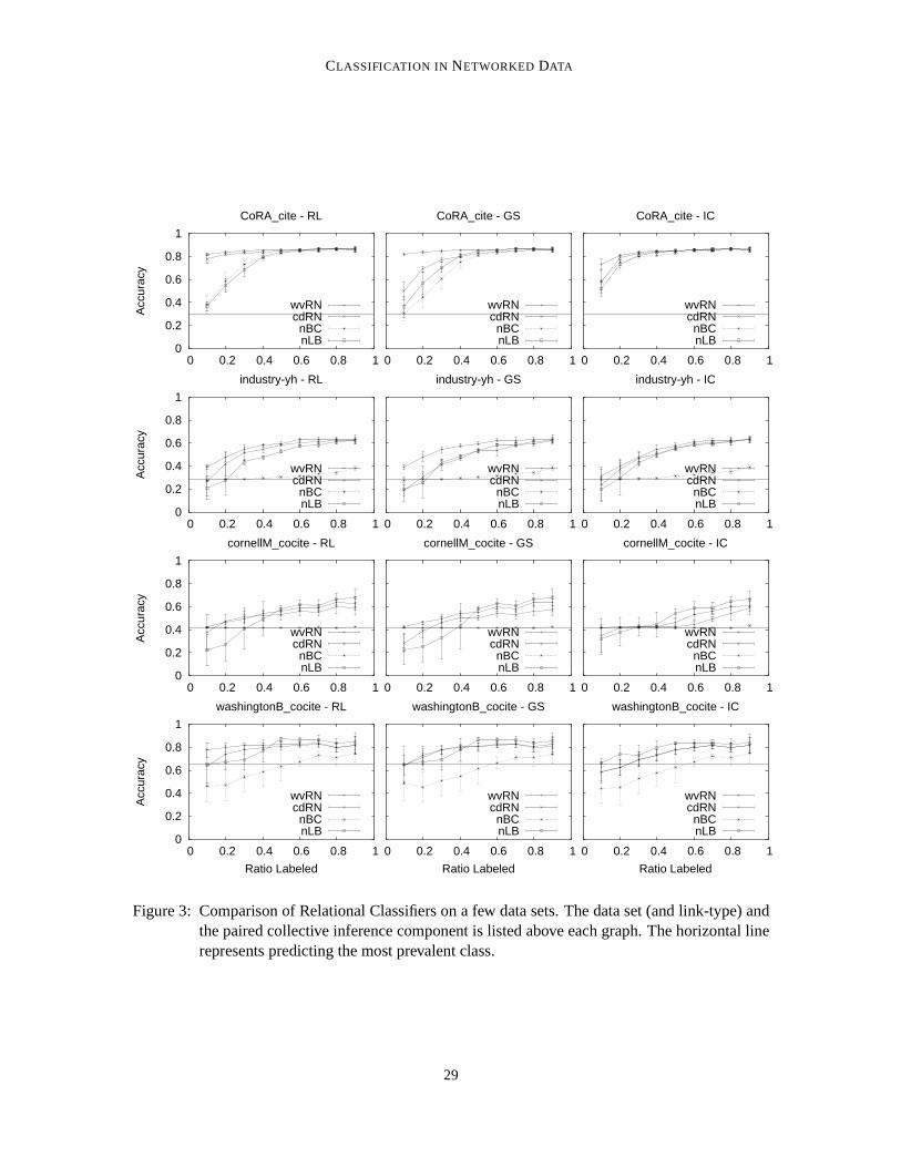
CLASSIFICATION IN NETWORKED DATA
0
0.2
0.4
0.6
0.8
1
0 0.2 0.4 0.6 0.8 1
Acc
urac
y
CoRA_cite - RL
wvRNcdRNnBCnLB
0
0.2
0.4
0.6
0.8
1
0 0.2 0.4 0.6 0.8 1
CoRA_cite - GS
wvRNcdRNnBCnLB
0
0.2
0.4
0.6
0.8
1
0 0.2 0.4 0.6 0.8 1
CoRA_cite - IC
wvRNcdRNnBCnLB
0
0.2
0.4
0.6
0.8
1
0 0.2 0.4 0.6 0.8 1
Acc
urac
y
industry-yh - RL
wvRNcdRNnBCnLB
0
0.2
0.4
0.6
0.8
1
0 0.2 0.4 0.6 0.8 1
industry-yh - GS
wvRNcdRNnBCnLB
0
0.2
0.4
0.6
0.8
1
0 0.2 0.4 0.6 0.8 1
industry-yh - IC
wvRNcdRNnBCnLB
0
0.2
0.4
0.6
0.8
1
0 0.2 0.4 0.6 0.8 1
Acc
urac
y
cornellM_cocite - RL
wvRNcdRNnBCnLB
0
0.2
0.4
0.6
0.8
1
0 0.2 0.4 0.6 0.8 1
cornellM_cocite - GS
wvRNcdRNnBCnLB
0
0.2
0.4
0.6
0.8
1
0 0.2 0.4 0.6 0.8 1
cornellM_cocite - IC
wvRNcdRNnBCnLB
0
0.2
0.4
0.6
0.8
1
0 0.2 0.4 0.6 0.8 1
Acc
urac
y
Ratio Labeled
washingtonB_cocite - RL
wvRNcdRNnBCnLB
0
0.2
0.4
0.6
0.8
1
0 0.2 0.4 0.6 0.8 1
Ratio Labeled
washingtonB_cocite - GS
wvRNcdRNnBCnLB
0
0.2
0.4
0.6
0.8
1
0 0.2 0.4 0.6 0.8 1
Ratio Labeled
washingtonB_cocite - IC
wvRNcdRNnBCnLB
Figure 3: Comparison of Relational Classifiers on a few data sets. The data set (and link-type) andthe paired collective inference component is listed above each graph. The horizontal linerepresents predicting the most prevalent class.
29

MACSKASSY AND PROVOST
sample ratio (r)0.10 0.20 0.30 0.40 0.50 0.60 0.70 0.80 0.90
wvRN v cdRN 0.025 0.200 0.050 0.100 0.025 0.025 0.010 0.002 0.001
wvRN v nBC 0.001 0.001 0.001 0.001 0.001 0.001 0.001 0.001 0.001
wvRN v nLB 0.001 0.001 0.001 0.005 0 .400 0 .005 0 .002 0 .001 0 .001cdRN v nBC 0.050 0.001 0.001 0.001 0.001 0.001 0.001 0.001 0.001
cdRN v nLB 0.010 0.001 0.010 0.200 0 .050 0 .001 0 .001 0 .001 0 .001nLB v nBC — 0.200 0.001 0.001 0.001 0.001 0.001 0.001 0.001
Table 14: p-values for the Wilcoxon Signed-Rank test. We compared the accuracies between pairsof RC components across all data sets and IC methods. For eachcell, bold text meansthat the first method was better than the second method and italic text means it was worse.The cells with ’—’ means there was no significant difference.
sample ratio (r)0.10 0.20 0.30 0.40 0.50 0.60 0.70 0.80 0.90 overall
cdRN 0.106 0.273 0.370 0.423 0.474 0.496 0.519 0.533 0.549 0.416nLB −0.049 0.039 0.206 0.354 0.508 0.573 0.587 0.609 0.609 0.382
wvRN 0.157 0.299 0.392 0.453 0.494 0.525 0.543 0.563 0.571 0.444
Table 15: Relative error reductions (ERREL) for each RC component across all data sets. Each cellshows the error reduction of the given method. The last column, overall, is the averageerror reduction for the methods across all sample ratios. Bold entries indicate the largestrelative error reduction for each sample ratio.
sample ratio (r)0.10 0.20 0.30 0.40 0.50 0.60 0.70 0.80 0.90 total
wvRN 7 4 4 6 4 4 2 1 2 34cdRN 5 8 6 2 1 0 0 1 1 24nLB 0 0 2 4 7 8 10 10 9 50
Table 16: Number of times each RC implementation was the bestacross the12 data sets.
(primarily because of the lack of training data). On the other hand, wvRN is potentially a very-high-bias classifier (it does not learn a relational model atall). The learning-based classifiers maywell perform better with large numbers of known labels if there are patterns beyond homophilyto be learned. As a worst case for wvRN, consider a bipartite graph between two classes. In aleave-one-out cross-validation, wvRN would be wrong on every prediction. The relational learnersshould notice the true pattern immediately. More generally, one should expect a pattern of curvescrossing with increasing numbers of known labels, similar to learning curves crossing (Perlich et al.,2003): lower variance methods (such as wvRN) should be preferable with fewer known labels; moreflexible learning methods should be preferable with more known labels (thus, more training data).
Figure 3 shows for four of the data sets the performances of the four RC implementations. Therows of graphs correspond to data sets and the columns to the three different collective inference
30
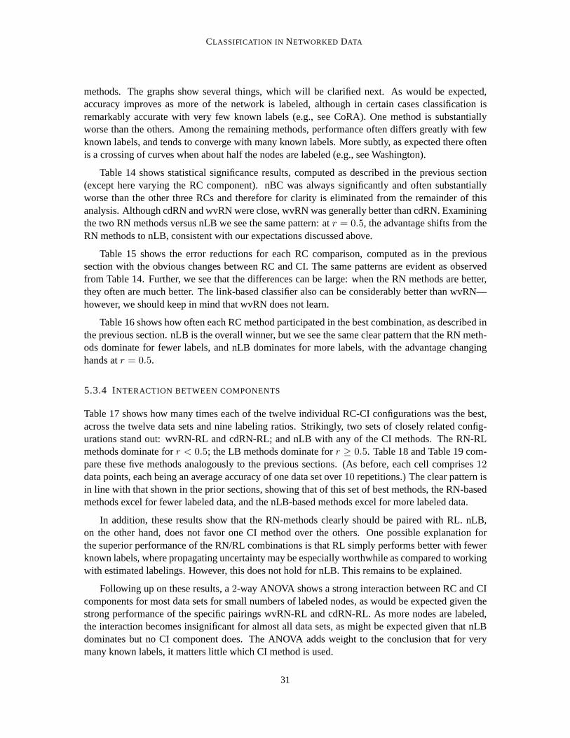
CLASSIFICATION IN NETWORKED DATA
methods. The graphs show several things, which will be clarified next. As would be expected,accuracy improves as more of the network is labeled, although in certain cases classification isremarkably accurate with very few known labels (e.g., see CoRA). One method is substantiallyworse than the others. Among the remaining methods, performance often differs greatly with fewknown labels, and tends to converge with many known labels. More subtly, as expected there oftenis a crossing of curves when about half the nodes are labeled (e.g., see Washington).
Table 14 shows statistical significance results, computed as described in the previous section(except here varying the RC component). nBC was always significantly and often substantiallyworse than the other three RCs and therefore for clarity is eliminated from the remainder of thisanalysis. Although cdRN and wvRN were close, wvRN was generally better than cdRN. Examiningthe two RN methods versus nLB we see the same pattern: atr = 0.5, the advantage shifts from theRN methods to nLB, consistent with our expectations discussed above.
Table 15 shows the error reductions for each RC comparison, computed as in the previoussection with the obvious changes between RC and CI. The same patterns are evident as observedfrom Table 14. Further, we see that the differences can be large: when the RN methods are better,they often are much better. The link-based classifier also can be considerably better than wvRN—however, we should keep in mind that wvRN does not learn.
Table 16 shows how often each RC method participated in the best combination, as described inthe previous section. nLB is the overall winner, but we see the same clear pattern that the RN meth-ods dominate for fewer labels, and nLB dominates for more labels, with the advantage changinghands atr = 0.5.
5.3.4 INTERACTION BETWEEN COMPONENTS
Table 17 shows how many times each of the twelve individual RC-CI configurations was the best,across the twelve data sets and nine labeling ratios. Strikingly, two sets of closely related config-urations stand out: wvRN-RL and cdRN-RL; and nLB with any of the CI methods. The RN-RLmethods dominate forr < 0.5; the LB methods dominate forr ≥ 0.5. Table 18 and Table 19 com-pare these five methods analogously to the previous sections. (As before, each cell comprises12data points, each being an average accuracy of one data set over10 repetitions.) The clear pattern isin line with that shown in the prior sections, showing that ofthis set of best methods, the RN-basedmethods excel for fewer labeled data, and the nLB-based methods excel for more labeled data.
In addition, these results show that the RN-methods clearlyshould be paired with RL. nLB,on the other hand, does not favor one CI method over the others. One possible explanation forthe superior performance of the RN/RL combinations is that RL simply performs better with fewerknown labels, where propagating uncertainty may be especially worthwhile as compared to workingwith estimated labelings. However, this does not hold for nLB. This remains to be explained.
Following up on these results, a2-way ANOVA shows a strong interaction between RC and CIcomponents for most data sets for small numbers of labeled nodes, as would be expected given thestrong performance of the specific pairings wvRN-RL and cdRN-RL. As more nodes are labeled,the interaction becomes insignificant for almost all data sets, as might be expected given that nLBdominates but no CI component does. The ANOVA adds weight to the conclusion that for verymany known labels, it matters little which CI method is used.
31
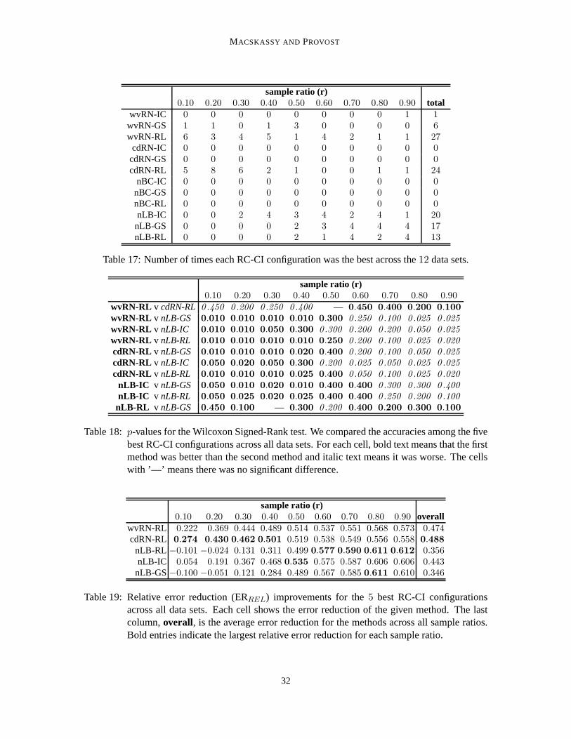
MACSKASSY AND PROVOST
sample ratio (r)0.10 0.20 0.30 0.40 0.50 0.60 0.70 0.80 0.90 total
wvRN-IC 0 0 0 0 0 0 0 0 1 1wvRN-GS 1 1 0 1 3 0 0 0 0 6wvRN-RL 6 3 4 5 1 4 2 1 1 27cdRN-IC 0 0 0 0 0 0 0 0 0 0cdRN-GS 0 0 0 0 0 0 0 0 0 0cdRN-RL 5 8 6 2 1 0 0 1 1 24
nBC-IC 0 0 0 0 0 0 0 0 0 0nBC-GS 0 0 0 0 0 0 0 0 0 0nBC-RL 0 0 0 0 0 0 0 0 0 0nLB-IC 0 0 2 4 3 4 2 4 1 20nLB-GS 0 0 0 0 2 3 4 4 4 17nLB-RL 0 0 0 0 2 1 4 2 4 13
Table 17: Number of times each RC-CI configuration was the best across the12 data sets.
sample ratio (r)0.10 0.20 0.30 0.40 0.50 0.60 0.70 0.80 0.90
wvRN-RL v cdRN-RL 0 .450 0 .200 0 .250 0 .400 — 0.450 0.400 0.200 0.100
wvRN-RL v nLB-GS 0.010 0.010 0.010 0.010 0.300 0 .250 0 .100 0 .025 0 .025wvRN-RL v nLB-IC 0.010 0.010 0.050 0.300 0 .300 0 .200 0 .200 0 .050 0 .025wvRN-RL v nLB-RL 0.010 0.010 0.010 0.010 0.250 0 .200 0 .100 0 .025 0 .020cdRN-RL v nLB-GS 0.010 0.010 0.010 0.020 0.400 0 .200 0 .100 0 .050 0 .025cdRN-RL v nLB-IC 0.050 0.020 0.050 0.300 0 .200 0 .025 0 .050 0 .025 0 .025cdRN-RL v nLB-RL 0.010 0.010 0.010 0.025 0.400 0 .050 0 .100 0 .025 0 .020
nLB-IC v nLB-GS 0.050 0.010 0.020 0.010 0.400 0.400 0 .300 0 .300 0 .400nLB-IC v nLB-RL 0.050 0.025 0.020 0.025 0.400 0.400 0 .250 0 .200 0 .100nLB-RL v nLB-GS 0.450 0.100 — 0.300 0 .200 0.400 0.200 0.300 0.100
Table 18: p-values for the Wilcoxon Signed-Rank test. We compared the accuracies among the fivebest RC-CI configurations across all data sets. For each cell, bold text means that the firstmethod was better than the second method and italic text means it was worse. The cellswith ’—’ means there was no significant difference.
sample ratio (r)0.10 0.20 0.30 0.40 0.50 0.60 0.70 0.80 0.90 overall
wvRN-RL 0.222 0.369 0.444 0.489 0.514 0.537 0.551 0.568 0.573 0.474cdRN-RL 0.274 0.430 0.462 0.501 0.519 0.538 0.549 0.556 0.558 0.488
nLB-RL −0.101 −0.024 0.131 0.311 0.499 0.577 0.590 0.611 0.612 0.356nLB-IC 0.054 0.191 0.367 0.468 0.535 0.575 0.587 0.606 0.606 0.443nLB-GS−0.100 −0.051 0.121 0.284 0.489 0.567 0.585 0.611 0.610 0.346
Table 19: Relative error reduction (ERREL) improvements for the5 best RC-CI configurationsacross all data sets. Each cell shows the error reduction of the given method. The lastcolumn,overall, is the average error reduction for the methods across all sample ratios.Bold entries indicate the largest relative error reductionfor each sample ratio.
32
CLASSIFICATION IN NETWORKED DATA
5.3.5 THE IMPORTANCE OFEDGE SELECTION
To create homogeneous graphs, we had to select the edges to use. As mentioned briefly above, thetype of edge selected can have a substantial impact on classification accuracy. For these data sets,the worst case (we have found) occurs for WebKB. As describedin Section 5.1.3, for the resultspresented so far we have used co-citation links, based on observations in prior published work. Anobvious alternative is to use the hyperlinks themselves.
Figures 4 and 5 show the results of using hyperlinks instead of co-citation links. Using hy-perlinks, the network-classification methods perform muchworse than with co-citations. Althoughthere is some lift at large values ofr, especially for the Washington data, the performance is notcomparable to that with the co-citation formulation. The transformation from the hyperlink-basednetwork to the co-citation-based network adds no new information to the graph. However, in thehyperlink formulation the network classification methods cannot take full advantage of the informa-tion present—mainly because of the stark violation of the first-order Markov assumption made bythe relational classifiers. These results demonstrate thatthe choice of edges can be crucial for goodperformance.
5.3.6 AUTOMATIC EDGE SELECTION
Creating a graph with a single type of edge from a problem where various possible links exist isa representation engineering problem reminiscent of the selection of a small set of useful featuresfor traditional classification.20 For feature selection, practitioners use a combination of domainknowledge and trial and error to select a good representation. To create the networked data for ourstudy, we chose edges based on suggestions from prior work—which indirectly combines domainknowledge and prior trial and error, although we explicitlyavoided choosing the representationsbased on their performance using NetKit.
Pursuing the analogy with choosing features, it may be possible to select edges automatically. Itis beyond the scope of this paper to address the general (openand important) problem of edge selec-tion; however, the excellence (on these data sets) and simplicity of wvRN suggests straightforwardtechniques.
If we consider the data sets used in the study, all but the industry classification data sets havemore than one type of edge:
1. cora: We linked entities through citations (cite). Alternatively, we could have linked by thesharing of an author (author), or by either relationship (combined as a single generic link).
2. imdb: There are many types of ways to connect two movies, but we focus here on four thatwere suggested to us by David Jensen:actor, director, producerand production company(prodco). Again, we could use any or all of them (we do not consider allpossible combina-tions here).
3. WebKB: Based on prior work, we chose co-citations (cocite) for the case study and latershowed that the original hyperlinks (hyper) were a poor choice.
20. We required a single edge type for our homogeneous case study; it is reasonable to conjecture that even if heteroge-neous links are allowed, a small set of good links would be preferable. For example, a link-based classifier producesa feature-vector representation with multiple positions per link type.
33
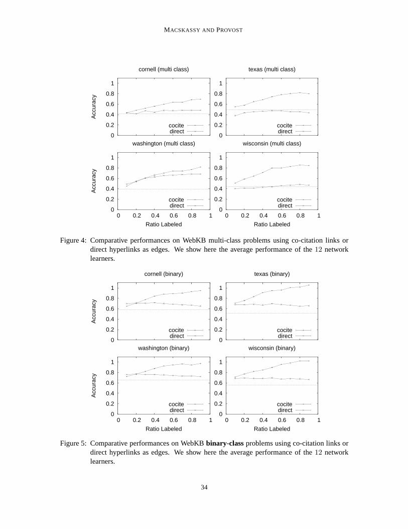
MACSKASSY AND PROVOST
0
0.2
0.4
0.6
0.8
1
0 0.2 0.4 0.6 0.8 1
Acc
urac
y
cornell (multi class)
cocitedirect
0
0.2
0.4
0.6
0.8
1
0 0.2 0.4 0.6 0.8 1
texas (multi class)
cocitedirect
0
0.2
0.4
0.6
0.8
1
0 0.2 0.4 0.6 0.8 1
Acc
urac
y
Ratio Labeled
washington (multi class)
cocitedirect
0
0.2
0.4
0.6
0.8
1
0 0.2 0.4 0.6 0.8 1
Ratio Labeled
wisconsin (multi class)
cocitedirect
Figure 4: Comparative performances on WebKB multi-class problems using co-citation links ordirect hyperlinks as edges. We show here the average performance of the12 networklearners.
0
0.2
0.4
0.6
0.8
1
0 0.2 0.4 0.6 0.8 1
Acc
urac
y
cornell (binary)
cocitedirect
0
0.2
0.4
0.6
0.8
1
0 0.2 0.4 0.6 0.8 1
texas (binary)
cocitedirect
0
0.2
0.4
0.6
0.8
1
0 0.2 0.4 0.6 0.8 1
Acc
urac
y
Ratio Labeled
washington (binary)
cocitedirect
0
0.2
0.4
0.6
0.8
1
0 0.2 0.4 0.6 0.8 1
Ratio Labeled
wisconsin (binary)
cocitedirect
Figure 5: Comparative performances on WebKBbinary-classproblems using co-citation links ordirect hyperlinks as edges. We show here the average performance of the12 networklearners.
34
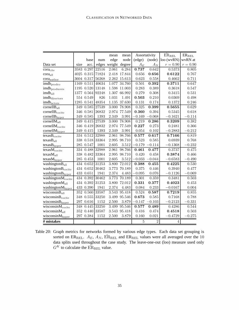
CLASSIFICATION IN NETWORKED DATA
mean mean Assortativity ERREL ERREL
base num edge node(edge) (node) loo (wvRN) wvRN atData set size acc. edges weight degree AE AN r = 0.90 r = 0.90coracite 3583 0.297 22516 2.061 6.284 0.737 0.642 0.5373 0.805coraall 4025 0.315 71824 2.418 17.844 0.656 0.656 0.6122 0.767coraauthor 3604 0.317 56268 2.262 15.613 0.623 0.558 0.4662 0.711imdbprodco 1169 0.511 40634 1.077 34.760 0.501 0.392 0.3711 0.647imdbproducers 1195 0.520 13148 1.598 11.003 0.283 0.389 0.3618 0.547imdball 1377 0.564 92248 1.307 66.992 0.279 0.308 0.3415 0.531imdbdirectors 554 0.549 826 1.031 1.491 0.503 0.210 0.0369 0.498imdbactors 1285 0.541 48354 1.135 37.630 0.131 0.174 0.1372 0.246cornellBall 349 0.585 27539 3.000 78.908 0.325 0.399 0.5655 0.629cornellBcocite 346 0.581 26832 2.974 77.549 0.360 0.394 0.5345 0.618cornellBhyper 349 0.585 1393 2.349 3.991 −0.169 −0.068 −0.1621 −0.114cornellMall 349 0.415 27539 3.000 78.908 0.219 0.286 0.3209 0.382cornellMcocite 346 0.419 26832 2.974 77.549 0.227 0.273 0.2481 0.366cornellMhyper 349 0.415 1393 2.349 3.991 0.054 0.102 −0.2883 −0.212texasBcocite 334 0.512 32988 2.961 98.766 0.577 0.617 0.7166 0.819texasBall 338 0.518 33364 2.995 98.710 0.523 0.585 0.6939 0.768texasBhyper 285 0.547 1001 2.605 3.512 −0.179 −0.114 −0.1368 −0.232texasMcocite 334 0.488 32988 2.961 98.766 0.461 0.477 0.3737 0.475texasMall 338 0.482 33364 2.995 98.710 0.420 0.458 0.3874 0.466texasMhyper 285 0.453 1001 2.605 3.512 −0.033 −0.044 −0.6583 −0.490washingtonBall 434 0.652 31253 3.800 72.012 0.388 0.455 0.4225 0.530washingtonBcocite 434 0.652 30462 3.773 70.189 0.375 0.446 0.3940 0.477washingtonBhyper 433 0.651 1941 2.374 4.483 −0.095 0.076 −0.1126 −0.069washingtonMcocite 434 0.392 30462 3.773 70.189 0.301 0.359 0.3481 0.503washingtonMall 434 0.392 31253 3.800 72.012 0.331 0.377 0.4023 0.453washingtonMhyper 433 0.390 1941 2.374 4.483 0.084 0.233 −0.0167 0.004wisconsinBall 352 0.560 33587 3.543 95.418 0.524 0.587 0.7219 0.855wisconsinBcocite 348 0.555 33250 3.499 95.546 0.673 0.585 0.7168 0.788wisconsinBhyper 297 0.616 1152 2.500 3.879 −0.147 −0.103 −0.2123 −0.331wisconsinMcocite 348 0.445 33250 3.499 95.546 0.577 0.489 0.4286 0.544wisconsinMall 352 0.440 33587 3.543 95.418 0.416 0.474 0.4518 0.503wisconsinMhyper 297 0.384 1152 2.500 3.879 0.160 0.021 −0.4729 −0.275
# mistakes 5 2 4
Table 20: Graph metrics for networks formed by various edge types. Each data set grouping issorted on ERREL. AE, AN , ERREL and ERREL values were all averaged over the10data splits used throughout the case study. The leave-one-out (loo) measure used onlyGK to calculate theERREL value.
35
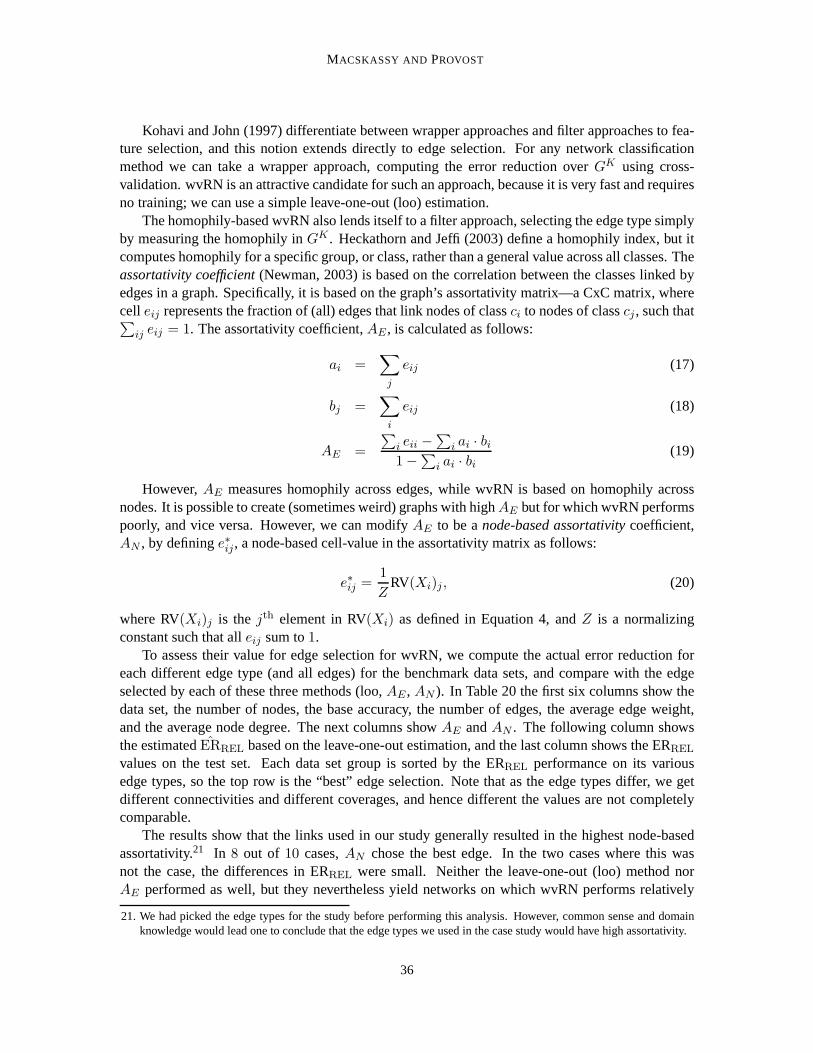
MACSKASSY AND PROVOST
Kohavi and John (1997) differentiate between wrapper approaches and filter approaches to fea-ture selection, and this notion extends directly to edge selection. For any network classificationmethod we can take a wrapper approach, computing the error reduction overGK using cross-validation. wvRN is an attractive candidate for such an approach, because it is very fast and requiresno training; we can use a simple leave-one-out (loo) estimation.
The homophily-based wvRN also lends itself to a filter approach, selecting the edge type simplyby measuring the homophily inGK . Heckathorn and Jeffi (2003) define a homophily index, but itcomputes homophily for a specific group, or class, rather than a general value across all classes. Theassortativity coefficient(Newman, 2003) is based on the correlation between the classes linked byedges in a graph. Specifically, it is based on the graph’s assortativity matrix—a CxC matrix, wherecell eij represents the fraction of (all) edges that link nodes of classci to nodes of classcj , such that∑
ij eij = 1. The assortativity coefficient,AE , is calculated as follows:
ai =∑
j
eij (17)
bj =∑
i
eij (18)
AE =
∑i eii −
∑i ai · bi
1−∑
i ai · bi
(19)
However,AE measures homophily across edges, while wvRN is based on homophily acrossnodes. It is possible to create (sometimes weird) graphs with highAE but for which wvRN performspoorly, and vice versa. However, we can modifyAE to be anode-based assortativitycoefficient,AN , by defininge∗ij, a node-based cell-value in the assortativity matrix as follows:
e∗ij =1
ZRV(Xi)j, (20)
where RV(Xi)j is the jth element in RV(Xi) as defined in Equation 4, andZ is a normalizingconstant such that alleij sum to1.
To assess their value for edge selection for wvRN, we computethe actual error reduction foreach different edge type (and all edges) for the benchmark data sets, and compare with the edgeselected by each of these three methods (loo,AE , AN ). In Table 20 the first six columns show thedata set, the number of nodes, the base accuracy, the number of edges, the average edge weight,and the average node degree. The next columns showAE andAN . The following column showsthe estimatedERREL based on the leave-one-out estimation, and the last column shows the ERREL
values on the test set. Each data set group is sorted by the ERREL performance on its variousedge types, so the top row is the “best” edge selection. Note that as the edge types differ, we getdifferent connectivities and different coverages, and hence different the values are not completelycomparable.
The results show that the links used in our study generally resulted in the highest node-basedassortativity.21 In 8 out of 10 cases,AN chose the best edge. In the two cases where this wasnot the case, the differences in ERREL were small. Neither the leave-one-out (loo) method norAE performed as well, but they nevertheless yield networks on which wvRN performs relatively
21. We had picked the edge types for the study before performing this analysis. However, common sense and domainknowledge would lead one to conclude that the edge types we used in the case study would have high assortativity.
36
CLASSIFICATION IN NETWORKED DATA
well. Notice that for IMDb, althoughdirector has the highestAE, it also has very low coverage(only 554 nodes were connected), and with such a slight difference in assortativity between thatandprodco there should be no question which should be used for classification.AN and the leave-one-out estimates are much more volatile thanAE as the amount of labeled data decreases, becausetypically there are many more edges than nodes. If we believethat assortativity is relatively stableacross the network, it may be beneficial to useAE when little is known. However, for our data sets,AN performs just as well asAE even whenr = 0.1.
In summary, these results show that the differences in the results by domain, and even withindomains, depend on the level of homophily. This is almost tautological for wvRN. We also com-puted many other graph statistics besides the homophily measures (e.g., average degree, number ofconnected clusters, graph diameter, shortest paths, etc.)none of which were as strongly correlatedwith performance.
5.3.7 NETWORK-ONLY CLASSIFICATION AS A BASELINE FOR RELATIONAL LEARNING
STUDIES
The foregoing results support the claim that network-only classification should be used as a baselineagainst which more sophisticated network-classification methods should be compared. Therefore,for example, when evaluating a system for the classificationof interconnected web pages, theirconnectivity alone should be considered in addition to their text alone. This of course is soundscientific methodology, requiring one to look for simpler explanations for a phenomenon once acomplex explanation has been found. When considering a sophisticated relational learning methodon networked data, using the network alone is one sort of lesion or ablation study (Langley, 2000).Our point here is that the absolute classification performance based only on the network of classlabels is remarkable in several of the cases examined above.For example, who would have thoughtthat on the University of Texas student/not-student classification task, accuracy could be increasedfrom 62.9% to 91.2% using just the network structure—with nolearning?
Nevertheless, it is enlightening to compare the these simple methods to alternatives. In thissection we provide several such comparisons. We compare to text-only methods and to a relationallearning technique that uses both local and relational information, and we see that one might be ledto be overly optimistic by comparing solely to local-only baselines. We also compare to a graph-based method that does not fall into the “node-centric” framework. Finally, we replicate a prior,published study, showing that conclusions would have changed if a network-only baseline had beenused.
In real networks, the amount of local information and its relevance to the classification task varywidely. In certain social network classification applications, for example in support of counterterror-ism, no information at all may be available about certain individuals other than their connections toothers (Tumulty, 2006). In applications such as fraud detection in telecommunications little reliableinformation may be available for potential fraudsters, beyond the calls they make (or as discussedabove, local information may be ignored for many individuals because network-only classificationworks so well). On the other hand, the text of certain web pages contains a bonanza of informationrelevant for classifying the topic of the web page.
For determining how much better can be done by using both the text and the interconnectivity in-formation, even for existing techniques and benchmark datasets, a definitive answer would involve acomparison of a large number of alternative relational learning systems on equal experimental foot-
37
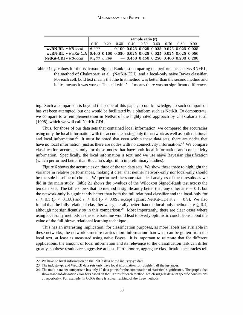
MACSKASSY AND PROVOST
sample ratio (r)0.10 0.20 0.30 0.40 0.50 0.60 0.70 0.80 0.90
wvRN-RL v NB-local 0 .200 — 0.100 0.025 0.025 0.025 0.025 0.025 0.025
wvRN-RL v NetKit-CDI 0.400 0.100 0.050 0.025 0.025 0.025 0.025 0.025 0.050
NetKit-CDI v NB-local 0 .400 0 .400 — 0.450 0.450 0.250 0.400 0.200 0.200
Table 21: p-values for the Wilcoxon Signed-Rank test comparing the performances of wvRN+RL,the method of Chakrabarti et al. (NetKit-CDI), and a local-only naive Bayes classifier.For each cell, bold text means that the first method was betterthan the second method anditalics means it was worse. The cell with ’—’ means there was no significant difference.
ing. Such a comparison is beyond the scope of this paper; to our knowledge, no such comparisonhas yet been attempted, but one would be facilitated by a platform such as NetKit. To demonstrate,we compare to a reimplementation in NetKit of the highly cited approach by Chakrabarti et al.(1998), which we will call NetKit-CDI.
Thus, for those of our data sets that contained local information, we compared the accuraciesusing only the local information with the accuracies using only the network as well as both relationaland local information.22 It must be noted that even within these data sets, there are nodes thathave no local information, just as there are nodes with no connectivity information.23 We compareclassification accuracies only for those nodes that have both local information and connectivityinformation. Specifically, the local information is text, and we use naive Bayesian classification(which performed better than Rocchio’s algorithm in preliminary studies).
Figure 6 shows the accuracies on three of the ten data sets. Weshow these three to highlight thevariance in relative performances, making it clear that neither network-only nor local-only shouldbe the sole baseline of choice. We performed the same statistical analyses of these results as wedid in the main study. Table 21 shows thep-values of the Wilcoxon Signed-Rank test across theten data sets. The table shows that no method is significantlybetter than any other atr = 0.1, butthe network-only is significantly better than both the full relational classifier and the local-only forr ≥ 0.3 (p ≤ 0.100) andr ≥ 0.4 (p ≤ 0.025 except against NetKit-CDI atr = 0.9). We alsofound that the fully relational classifier was generally better than the local-only method atr ≥ 0.4,although not significantly so in this comparison.24 Most importantly, there are clear cases whereusing local-only methods as the sole baseline would lead to overly optimistic conclusions about thevalue of the full-blown relational learning technique.
This has an interesting implication: for classification purposes, as more labels are available inthese networks, the network structure carries more information than what can be gotten from thelocal text, at least as measured using naive Bayes. It is important to reiterate that for differentapplications, the amount of local information and its relevance to the classification task can differgreatly, so these results are suggestive at best. Furthermore, aggregate classification accuracies tell
22. We have no local information on the IMDb data or the industry-yh data.23. The industry-pr and WebKB data sets only have local information for roughly half the instances.24. The multi-data-set comparison has only 10 data points for the computation of statistical significance. The graphs also
show standard-deviation error bars based on the 10 runs for each method, which suggest data-set specific conclusionsof superiority. For example, in CoRA there is a clear rankingof the three methods.
38
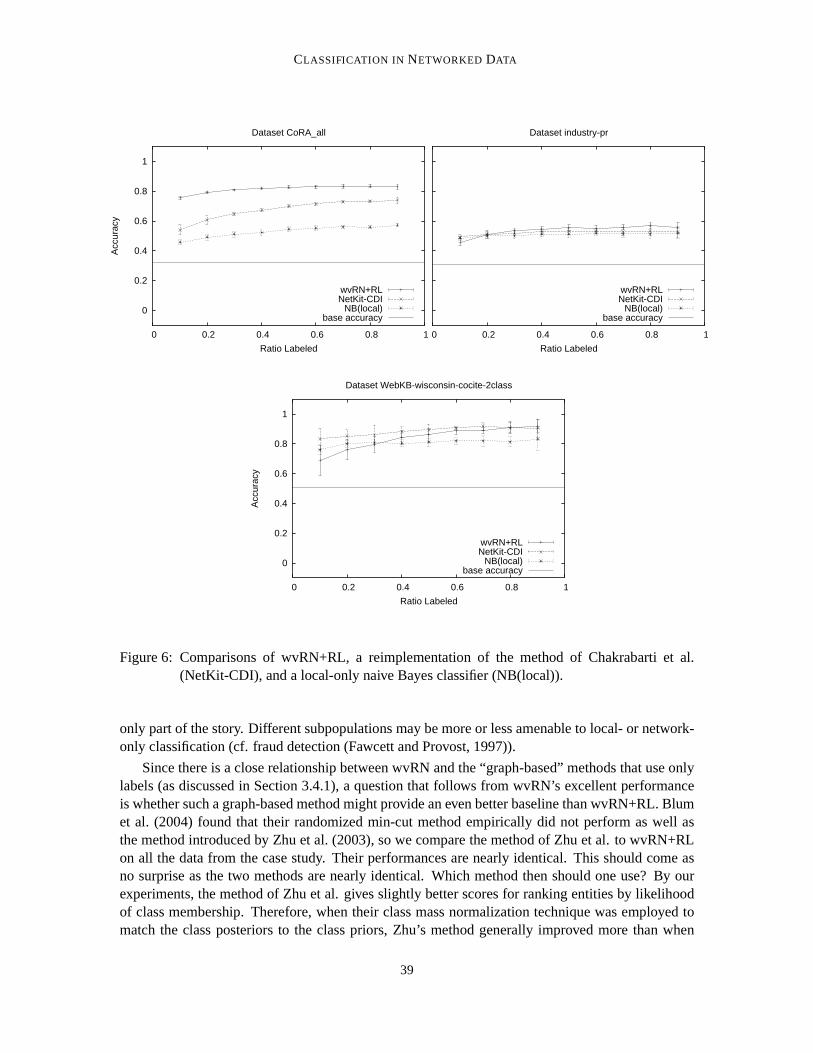
CLASSIFICATION IN NETWORKED DATA
0
0.2
0.4
0.6
0.8
1
0 0.2 0.4 0.6 0.8 1
Acc
urac
y
Ratio Labeled
Dataset CoRA_all
wvRN+RLNetKit-CDI
NB(local)base accuracy
0 0.2 0.4 0.6 0.8 1
Ratio Labeled
Dataset industry-pr
wvRN+RLNetKit-CDI
NB(local)base accuracy
0
0.2
0.4
0.6
0.8
1
0 0.2 0.4 0.6 0.8 1
Acc
urac
y
Ratio Labeled
Dataset WebKB-wisconsin-cocite-2class
wvRN+RLNetKit-CDI
NB(local)base accuracy
Figure 6: Comparisons of wvRN+RL, a reimplementation of themethod of Chakrabarti et al.(NetKit-CDI), and a local-only naive Bayes classifier (NB(local)).
only part of the story. Different subpopulations may be moreor less amenable to local- or network-only classification (cf. fraud detection (Fawcett and Provost, 1997)).
Since there is a close relationship between wvRN and the “graph-based” methods that use onlylabels (as discussed in Section 3.4.1), a question that follows from wvRN’s excellent performanceis whether such a graph-based method might provide an even better baseline than wvRN+RL. Blumet al. (2004) found that their randomized min-cut method empirically did not perform as well asthe method introduced by Zhu et al. (2003), so we compare the method of Zhu et al. to wvRN+RLon all the data from the case study. Their performances are nearly identical. This should come asno surprise as the two methods are nearly identical. Which method then should one use? By ourexperiments, the method of Zhu et al. gives slightly better scores for ranking entities by likelihoodof class membership. Therefore, when their class mass normalization technique was employed tomatch the class posteriors to the class priors, Zhu’s methodgenerally improved more than when
39
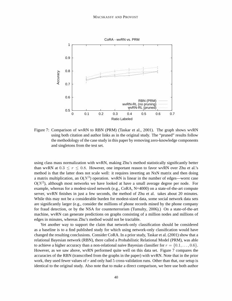
MACSKASSY AND PROVOST
0.5
0.6
0.7
0.8
0.9
1
0 0.1 0.2 0.3 0.4 0.5 0.6 0.7
Acc
urac
y
Ratio Labeled
CoRA - wvRN vs. PRM
RBN (PRM)wvRN-RL (no pruning)
wvRN-RL (pruned)
Figure 7: Comparison of wvRN to RBN (PRM) (Taskar et al., 2001). The graph shows wvRNusing both citation and author links as in the original study. The “pruned” results followthe methodology of the case study in this paper by removing zero-knowledge componentsand singletons from the test set.
using class mass normalization with wvRN, making Zhu’s method statistically significantly betterthan wvRN at0.3 ≤ r ≤ 0.8. However, one important reason to favor wvRN over Zhu et al.’smethod is that the latter does not scale well: it requires inverting an NxN matrix and then doinga matrix multiplication, an O(N3) operation. wvRN is linear in the number of edges—worst caseO(N2), although most networks we have looked at have a small average degree per node. Forexample, whereas for a modest-sized network (e.g., CoRA, N=4000) on a state-of-the-art computeserver, wvRN finishes in just a few seconds, the method of Zhu et al. takes about 20 minutes.While this may not be a considerable burden for modest-sizeddata, some social network data setsare significantly larger (e.g., consider the millions of phone records mined by the phone companyfor fraud detection, or by the NSA for counterterrorism (Tumulty, 2006).) On a state-of-the-artmachine, wvRN can generate predictions on graphs consisting of a million nodes and millions ofedges in minutes, whereas Zhu’s method would not be tractable.
Yet another way to support the claim that network-only classification should be consideredas a baseline is to a find published study for which using network-only classification would havechanged the resulting conclusions. Consider CoRA. In a prior study, Taskar et al. (2001) show that arelational Bayesian network (RBN), there called a Probabilistic Relational Model (PRM), was ableto achieve a higher accuracy than a non-relational naive Bayesian classifier forr = {0.1, . . . , 0.6}.However, as we saw above, wvRN performed quite well on this data set. Figure 7 compares theaccuracies of the RBN (transcribed from the graphs in the paper) with wvRN. Note that in the priorwork, they used fewer values ofr and only had5 cross-validation runs. Other than that, our setup isidentical to the original study. Also note that to make a direct comparison, we here use both author
40
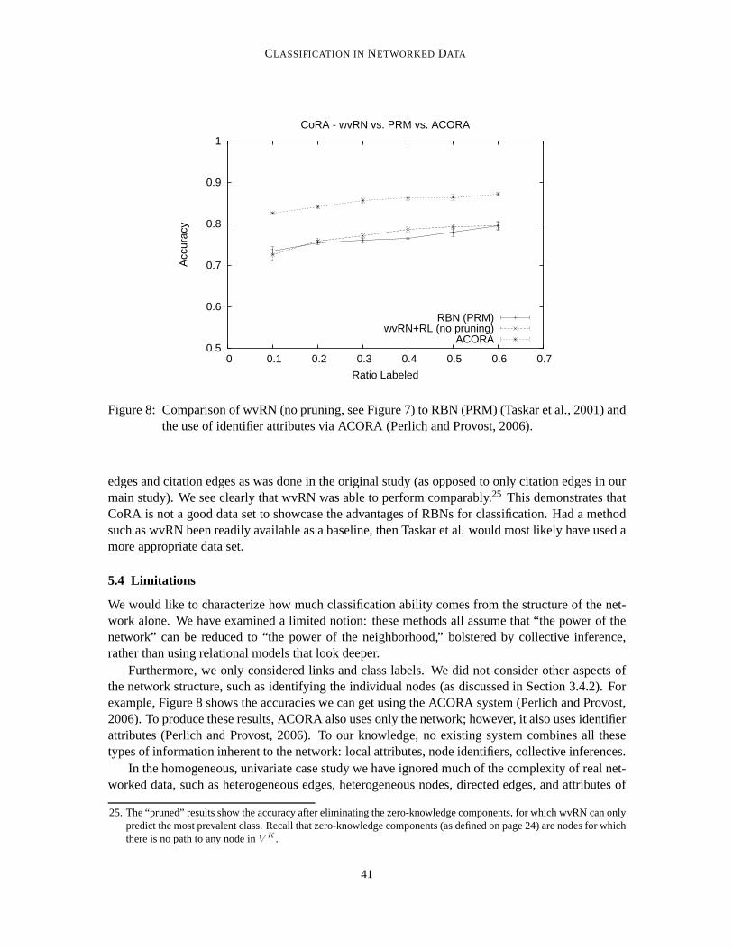
CLASSIFICATION IN NETWORKED DATA
0.5
0.6
0.7
0.8
0.9
1
0 0.1 0.2 0.3 0.4 0.5 0.6 0.7
Acc
urac
y
Ratio Labeled
CoRA - wvRN vs. PRM vs. ACORA
RBN (PRM)wvRN+RL (no pruning)
ACORA
Figure 8: Comparison of wvRN (no pruning, see Figure 7) to RBN(PRM) (Taskar et al., 2001) andthe use of identifier attributes via ACORA (Perlich and Provost, 2006).
edges and citation edges as was done in the original study (asopposed to only citation edges in ourmain study). We see clearly that wvRN was able to perform comparably.25 This demonstrates thatCoRA is not a good data set to showcase the advantages of RBNs for classification. Had a methodsuch as wvRN been readily available as a baseline, then Taskar et al. would most likely have used amore appropriate data set.
5.4 Limitations
We would like to characterize how much classification ability comes from the structure of the net-work alone. We have examined a limited notion: these methodsall assume that “the power of thenetwork” can be reduced to “the power of the neighborhood,” bolstered by collective inference,rather than using relational models that look deeper.
Furthermore, we only considered links and class labels. We did not consider other aspects ofthe network structure, such as identifying the individual nodes (as discussed in Section 3.4.2). Forexample, Figure 8 shows the accuracies we can get using the ACORA system (Perlich and Provost,2006). To produce these results, ACORA also uses only the network; however, it also uses identifierattributes (Perlich and Provost, 2006). To our knowledge, no existing system combines all thesetypes of information inherent to the network: local attributes, node identifiers, collective inferences.
In the homogeneous, univariate case study we have ignored much of the complexity of real net-worked data, such as heterogeneous edges, heterogeneous nodes, directed edges, and attributes of
25. The “pruned” results show the accuracy after eliminating the zero-knowledge components, for which wvRN can onlypredict the most prevalent class. Recall that zero-knowledge components (as defined on page 24) are nodes for whichthere is no path to any node inV K .
41

MACSKASSY AND PROVOST
nodes and edges. Each of these introduces complications andopportunities for modeling. Thereare no comprehensive, empirical machine learning studies that consider these dimensions system-atically. For example, when using attributes of nodes, how much is gained by using them in therelational classifier, as opposed to using them simply to initialize priors? (For example, Chakrabartiet al. (1998) found that using the text of hyperlinked documents reduced performance.) Similarly,how much value is added by considering multiple edge types explicitly?
An important limitation of this work, with respect to its relevance to practical problems, isthat we choose training data randomly to be labeled. It is likely that the data for which labels areavailable are interdependent. For example, all the membersfrom one terrorist cell may be knownand none from another. If other attributes are available more uniformly, then studies such as thismay artificially favor network-only methods over attribute-based methods.
5.5 Conclusions and Future Work
We introduced a modular toolkit, NetKit-SRL, for classification in networked data. The importanceof NetKit is three-fold: (1) it generalizes several existing methods for classification in networkeddata, thereby making comparison to existing methods possible; (2) it enables the creation and use ofmany new algorithms by its modularity and extensibility, and (3) it enables the analysis/comparisonof individual components and configurations.
We used NetKit to perform a case study of within-network, univariate classification for homo-geneous networked data. The case study makes several contributions. It provides demonstrativesupport for points 2 and 3 above. Five network classifiers stood clearly above the rest, and three ofthem were novel combinations of components. Certain collective inference and relational classifica-tion components stand out with consistently better performance: for collective inference, relaxationlabeling was best; for relational classification, the link-based classifier clearly was preferable whenmany labels were known. The lower-variance methods (wvRN and cdRN) dominated when fewerlabels were known. In combination, two pairs of RC-CI combinations stand out strikingly: nLBwith any of the collective inference methods dominates whenmany labels are known; the relationalneighbor methods with relaxation labeling (wvRN-RL and cdRN-RL) dominate when fewer labelsare known. Of particular interest given this latter result,we also show the close correspondenceof several simple, network classification methods: the node-centric wvRN-RL, the whole-graphGaussian-field method of Zhu et al. (2003), and classic connectionist techniques such as Hopfieldnetworks (Hopfield, 1982).
More generally, the results showcase two different modes ofwithin-network classification thatcall for different types of methods: when many labels are known versus when few labels are known.These modes correspond to different application scenarios. The former may correspond (for ex-ample) to networks that evolve over time with new nodes needing classification before their labelsbecome known naturally, as would be the case for predicting movie box-office receipts. Examplesof the little-known scenario can be found in counter-terrorism and law enforcement, where analystsform complex interaction networks containing a few, known bad guys. The little-known scenariohas an economic component, similar to active learning: it may be worthwhile to incur costs to la-bel additional nodes in the network, because this will lead to much improved classification. Thissuggests another direction for future work—identifying the most beneficial nodes for labeling (cf.,Domingos and Richardson (2001)).
42
CLASSIFICATION IN NETWORKED DATA
The case study also showcases a problem of representation for network classification: the selec-tion of which edges to use. It is straightforward to extend NetKit’s relational classification methodsto handle heterogeneous links. However, that would not solve the fundamental problem that edgeselection, like feature selection for traditional learning, may improve generalization performance(as well as provide simpler models).
Finally, the case study demonstrates the power of simple network classification models. Onthe benchmark data sets, error rates were reduced markedly by taking into account only the class-linkage structure of the network. Although learning helpedin many cases, the no-learning wvRNwas a very strong competitor—performing very well especially when few labels were known. Thisargues strongly for using simple, network-only models as baselines in studies of classification innetworked data. This result was supported further by followup analyses showing cases where onewould draw overly optimistic conclusions about the value ofmore-sophisticated methods if thesenetwork-only techniques were not used as baselines. It alsoraises the question of whether we need“better” benchmark data sets—to showcase the value of more-powerful techniques.
Classification in networked data is important for real-world applications, and presents manyopportunities for machine-learning research. The field is beginning to amass benchmark domainscontaining networked data. We hope that NetKit can facilitate systematic study.
Acknowledgments
David Jensen made many helpful suggestions, including pointing us to the WebKB data set and sug-gesting ways to do well on it. Abraham Bernstein collaborated on the generation of the two industryclassification data sets. Kaveh R. Ghazi worked diligently coding the open-source NetKit and en-suring that it would be ready for release on schedule. We thank Ben Taskar and Andrew McCallumfor providing us with versions of the Cora data set. Thanks toSugato Basu, Misha Bilenko, PedroDomingos, Joydeep Ghosh, David Jensen, Yann LeCun, Andrew McCallum, Jennifer Neville, MarkNewman, Claudia Perlich, and audience members of talks for helpful comments and discussions.Finally, we thank Andrew McCallum and the anonymous reviewers who helped to strengthen thepaper considerably.
This work was funded in part by a grant from the New York Software Industry Association.This research also was sponsored in part by the Air Force Research Laboratory, Air Force MaterielCommand, USAF, under Agreement number F30602-01-2-0585. The views and conclusions con-tained herein are those of the authors and should not be interpreted as necessarily representing theofficial policies or endorsements, either expressed or implied, of AFRL or the U.S. Government.
References
J. C. Almack. The Influence of Intelligence on the Selection of Associates.School and Society, 16:529–530, 1922.
A. Bernstein, S. Clearwater, S. Hill, C. Perlich, and F. Provost. Discovering Knowledge fromRelational Data Extracted from Business News. InProceedings of the Multi-Relational DataMining Workshop (MRDM) at the Eighth ACM SIGKDD International Conference on KnowledgeDiscovery and Data Mining, 2002.
A. Bernstein, S. Clearwater, and F. Provost. The RelationalVector-space Model and Industry Clas-sification. InProceedings of the Learning Statistical Models from Relational Data Workshop
43

MACSKASSY AND PROVOST
(SRL) at the 19th International Joint Conference on Artificial Intelligence (IJCAI), pages 8–18,2003.
J. Besag. Spatial interaction and the statistical analysisof lattice systems.Journal of the RoyalStatistical Society, 36(2):192–236, 1974.
J. Besag. On the statistical analysis of dirty pictures.Journal of the Royal Statistical Society, 48(3):259–302, 1986.
P. M. Blau. Inequality and Heterogeneity: A Primitive Theory of SocialStructure. New York: FreePress, 1977.
A. Blum and S. Chawla. Learning from Labeled and Unlabeled Data using Graph Mincuts. InProceedings of the International Conference on Machine Learning (ICML), pages 19–26, 2001.
A. Blum, J. Lafferty, R. Reddy, and M. R. Rwebangira. Semi-supervised learning using randomizedmincuts. InProceedings of the 21st International Conference on Machine Learning (ICML),2004.
H. Bott. Observation of Play Activities in a Nursery School.Genetic Psychology Monographs, 4:44–88, 1928.
Y. Boykov, O. Veksler, and R. Zabih. Fast Approximate EnergyMinimization via Graph Cuts.IEEETransactions on Pattern Analysis and Machine Intellingence (PAMI), 23(11), November 2001.
S. Chakrabarti, B. Dom, and P. Indyk. Enhanced Hypertext Categorization Using Hyperlinks. InACM SIGMOD International Conference on Management of Data, 1998.
C. Cortes, D. Pregibon, and C. T. Volinsky. Communities of Interest. InProceedings of IntelligentData Analysis (IDA), 2001.
R. G. Cowell, A. P. Dawid, S. L. Lauritzen, and D. J. Spiegelhalter. Probabilistic networks andexpert systems. Springer, 1999.
M. Craven, D. Freitag, A. McCallum, T. Mitchell, K. Nigam, and C. Y. Quek. Learning to ExtractSymbolic Knowledge from the World Wide Web. In15th Conference of the American Associa-tion for Artificial Intelligence, 1998.
L. De Raedt, H. Blockeel, L. Dehaspe, and W. Van Laer. Three companions for data mining in firstorder logic. In Saso Dzeroski and Nada Lavrac, editors,Relational Data Mining, pages 105–139.Springer-Verlag, 2001.
I. S. Dhillon. Co-clustering documents and words using bipartite spectral graph partitioning. InKnowledge Discovery and Data Mining, pages 269–274, 2001.
R. L. Dobrushin. The Description of a Random Field by Means ofConditional Probabilities andConditions of its Regularity.Theory of Probability and its Application, 13(2):197–224, 1968.
P. Domingos and M. Richardson. Mining the network value of customers. InProceedings of theSeventh ACM SIGKDD International Conference on Knowledge Discovery and Data Mining,pages 57–66. CA: ACM Press, 2001.
44
CLASSIFICATION IN NETWORKED DATA
S. Dzeroski and N. Lavrac.Relational Data Mining. Berlin; New York: Springer, 2001.
W. Emde and D. Wettschereck. Relational Instance-Based Learning. In Lorenza Saitta, editor,Proceedings of the 13th International Conference on Machine Learning (ICML), pages 122–130.Morgan Kaufmann, 1996.
T. Fawcett and F. Provost. Adaptive fraud detection.Data Mining and Knowledge Discovery, 3:291–316, 1997.
T. Fawcett and F. Provost. Activity monitoring: Noticing interesting changes in behavior. InPro-ceedings of the Fifth ACM SIGKDD International Conference on Knowledge Discovery and DataMining, 1999.
P. A. Flach and N. Lachiche. 1BC: A First-Order Bayesian Classifier. In Saso Dzeroski and Peter A.Flach, editors,Proceedings of the Ninth International Workshop on Inductive Logic Programming(ILP), volume 1634, pages 92–103. Springer-Verlag, June 1999.
N. Friedman, L. Getoor, D. Koller, and A. Pfeffer. Learning Probabilistic Relational Models. InSixteenth International Joint Conference on Artificial Intelligence (IJCAI), 1999.
A. Galstyan and P. Cohen. Is Guilt by Association a Bad Thing?In Proceedings of the IntelligenceAnalysis Conference (IA), 2005.
S. Geman and D. Geman. Stochastic relaxation, Gibbs distributions and the Bayesian restoration ofimages.IEEE Transactions on Pattern Analysis and Machine Intellingence (PAMI), 6:721–741,1984.
W. R. Gilks, S. Richardson, and D. J. Spiegelhalter.Markov Chain Monte Carlo in Practice. Chap-man & Hall/CRC, 1995.
D. Greig, B. Porteous, and A. Seheult. Exact Maximum A Posteriori Estimation for Binary Images.J. Royal Statistical Soc., 51(2):271–279, 1989.
D. D. Heckathorn and J. Jeffi. Jazz networks: Using respondent-driven sampling to study stratifica-tion in two jazz musician communities. InAmerican Sociological Association meetings, August2003.
D. Heckerman, D. M. Chickering, C. Meek, R. Rounthwaite, andC. Kadie. Dependency Networksfor Inference, Collaborative Filtering, and Data Visualization. Journal of Machine LearningResearch (JMLR), 1:49–75, October 2000.
S. Hill, F. Provost, and C. Volinsky. Network-based Marketing: Identifying Likely Adopters viaConsumer Networks.Statistical Science, 22(2), May 2006.
G. E. Hinton and T. J. Sejnowski. Learning and Relearning in Boltzmann Machines.ParallelDistributed Processing: Explorations in the Microstructure of Cognition, 1: Foundations:282–317, 1986.
J. J. Hopfield. Neural networks and physical systems with emergent collective computational abil-ities. Proceedings of the National Academy of Sciences of the USA, 79(8):2554–2558, April1982.
45

MACSKASSY AND PROVOST
Z. Huang, H. Chen, and D. Zeng. Applying Associative Retrieval Techniques to Alleviate theSparsity Problem in Collaborative Filtering.ACM Transactions on Information Systems (TOIS),22(1), 2004.
R. A. Hummel and S. W. Zucker. On the foundations of relaxation labeling processes.IEEETransactions on Pattern Analysis and Machine Intelligence, 5(3):267–287, 1983.
E. Ising. Beitrag zur Theorie des Ferromagnetismus.Zeitschrift f. Physik, 31:253–258, 1925.[German].
David Jensen and Jennifer Neville. Data Mining in Social Networks. In National Academy ofSciences workshop on Dynamic Social Network Modeling and Analysis, 2002a.
D. Jensen and J. Neville. Linkage and Autocorrelation CauseFeature Selection Bias in RelationalLearning. InProceedings of the 19th International Conference on Machine Learning (ICML),2002b.
D. Jensen, J. Neville, and B. Gallagher. Why Collective Inference Improves Relational Classi-fication. In Proceedings of the 10th ACM SIGKDD International Conference on KnowledgeDiscovery and Data Mining, 2004.
T. Joachims. Transductive Learning via Spectral Graph Partitioning. In Proceedings of the Interna-tional Conference on Machine Learning (ICML), 2003.
J. Kleinberg andE. Tardos. Approximation Algorithms for Classification Problems with PairwiseRelations: Metric Labeling and Markov Random Fields. InIEEE Symposium on Foundations ofComputer Science, pages 14–23, 1999.
R. Kohavi and G. John. Wrappers for Feature Subset Selection. Artificial Intelligence special issueon Relevance, 97(1–2):273–324, 1997.
D. Koller and A. Pfeffer. Probabilistic Frame-Based Systems. InAAAI/IAAI, pages 580–587, 1998.
S. Kramer, N. Lavrac, and P. Flach. Propositionalization approaches to relational data mining.In Saso Dzeroski and Nada Lavrac, editors,Relational Data Mining, pages 262–291. Springer-Verlag, 2001.
J. Lafferty, A. McCallum, and F. Pereira. Conditional Random Fields: Probabilistic Models forSegmenting and Labeling Sequence Data. InProceedings of the 18th International Conferenceon Machine Learning (ICML), 2001.
P. Langley. Crafting Papers on Machine Learning. InProceedings of the 17th International Confer-ence on Machine Learning, pages 1207–1212. Morgan Kaufmann, San Francisco, CA, 2000.
P. Lazarsfeld and Robert K. Merton. Friendship as a Social Process: A Substantive and Method-ological Analysis. In Morroe Berger, Theodore Abel, and Charles H. Page, editors,Freedom andControl in Modern Society, pages 18–66. Van Nostrand, 1954.
C. P. Loomis. Political and Occupational Cleavages in a Hanoverian Village. Sociometry, 9:316–3333, 1946.
46
CLASSIFICATION IN NETWORKED DATA
Q. Lu and L. Getoor. Link-Based Classification. InProceedings of the 20th International Confer-ence on Machine Learning (ICML), 2003.
S. A. Macskassy and F. Provost. A Simple Relational Classifier. In Proceedings of the Multi-Relational Data Mining Workshop (MRDM) at the Ninth ACM SIGKDD International Conferenceon Knowledge Discovery and Data Mining, 2003.
S. A. Macskassy and F. Provost. Classification in Networked Data: A toolkit and a univariate casestudy. Technical Report CeDER Working Paper 04-08, Stern School of Business, New YorkUniversity, 2004.
S. A. Macskassy and F. Provost. Suspicion scoring based on guilt-by-association, collective infer-ence, and focused data access. InInternational Conference on Intelligence Analysis, 2005.
A. McCallum, K. Nigam, J. Rennie, and K. Seymore. Automatingthe Construction of InternetPortals with Machine Learning.Information Retrieval, 3(2):127–163, 2000.
M. McPherson, L. Smith-Lovin, and J. M. Cook. Birds of a Feather: Homophily in Social Networks.Annual Review of Sociology, 27:415–444, 2001.
K. Murphy, Y. Weiss, and M. I. Jordan. Loopy Belief-propagation for Approximate Inference: AnEmpirical Study. In K. B. Laskey and H. Prade, editors,Proceedings of the Fifteenth Conferenceon Uncertainty in Artificial Intelligence (UAI). Morgan Kaufmann, 1999.
J. Neville and D. Jensen. Iterative Classification in Relational Data. InAAAI Workshop on LearningStatistical Models from Relational Data, pages 13–20, 2000.
J. Neville and D. Jensen. Collective Classification with Relational Dependency Networks. InPro-ceedings of the Second Workshop on Multi-Relational Data Mining (MRDM-2003) at KDD-2003,2003.
J. Neville and D. Jensen. Dependency Networks for Relational Data. InProceedings of the FourthIEEE International Conference in Data Mining (ICDM), 2004.
J. Neville and D. Jensen. Leveraging Relational Autocorrelation with Latent Group Models. InProceedings of the IEEE International Conference on Data Mining (ICDM), 2005.
J. Neville, D. Jensen, L. Friedland, and M. Hay. Learning Relational Probability Trees. InProceed-ings of the Ninth ACM SIGKDD International Conference on Knowledge Discovery and DataMining, 2003.
J. Neville, O. Simsek, D. Jensen, J. Komoroske, K. Palmer, and H. Goldberg. Using relationalknowledge discovery to prevent securities fraud. InProceedings of the 11th ACM SIGKDDInternational Conference on Knowledge Discovery and Data Mining, 2005.
M. E. J. Newman. Mixing patterns in networks.Physical Review E, 67, 2003. 026126.
J. Pearl.Probabilistic Reasoning in Intelligent Systems. Morgan Kaufmann, 1988.
C. Perlich. Citation-Based Document Classification. InWorkshop on Information Technology andSystems (WITS), 2003.
47

MACSKASSY AND PROVOST
C. Perlich and F. Provost. Aggregation-based feature invention and relational concept classes. InKDD, 2003.
C. Perlich and F. Provost. Distribution-based aggregationfor relational learning with identifierattributes.Machine Learning, 62(1/2):65–105, 2006.
C. Perlich, F. Provost, and J. Simonoff. Tree induction vs. logistic regression: A learning-curveanalysis.Journal of Machine Learning Research, 2003.
A. Popescul and L. H. Ungar. Statistical Relational Learning for Link Prediction. InProceedings ofthe Learning Statistical Models from Relational Data Workshop (SRL) at the 19th InternationalJoint Conference on Artificial Intelligence (IJCAI), 2003.
R. B. Potts. Some generalized order-disorder transformations.Proceedings of the Cambridge Philo-sophic Society, 48:106–109, 1952.
F. Provost, C. Perlich, and S. A. Macskassy. Relational Learning Problems and Simple Models. InProceedings of the Learning Statistical Models from Relational Data Workshop (SRL) at the 19thInternational Joint Conference on Artificial Intelligence(IJCAI), pages 116–120, 2003.
H. M. Richardson. Community of Values as a Factor in Friendships of College and Adult Women.Journal of Social Psychology, 11:303–312, 1940.
M. Richardson and P. Domingos. Markov logic networks.Machine Learning, 62(1/2):107–136,2006.
J. Rocchio. Relevance feedback in information retrieval. In Salton, editor,The SMART RetrievalSystem: Experiments in Automatic Document Processing, chapter 14, pages 313–323. Prentice–Hall, 1971.
A. Rosenfeld, R. Hummel, and S. Zucker. Scene labeling by relaxation operations.IEEE Transac-tions on Systems, Man and Cybernetics, 6:420–433, 1976.
L. J. Savage.The Foundations of Statistics. John Wiley and Sons, 1954.
E. Segal, H. Wang, and D. Koller. Discovering molecular pathways from protein interaction andgene expression data.Bioinformatics, 19:I264–I272, Jul 2003a.
E. Segal, R. Yelensky, and D. Koller. Genome-wide discoveryof transcriptional modules from DNAsequence and gene expression.Bioinformatics, 19:I273–I282, Jul 2003b.
B. Taskar, E. Segal, and D. Koller. Probabilistic Classification and Clustering in Relational Data. InProceedings of the 17th International Joint Conference on Artificial Intelligence (IJCAI), pages870–878, 2001.
B. Taskar, P. Abbeel, and D. Koller. Discriminative Probabilistic Models for Relational Data. InEighteenth Conference on Uncertainty in Artificial Intelligence (UAI), August 2002.
B. Taskar, V. Chatalbashev, and D. Koller. Learning Associative Markov Networks. InProceedingsof the 21st International Conference on Machine Learning (ICML), July 2004.
48

CLASSIFICATION IN NETWORKED DATA
K. Tumulty. Inside Bush’s Secret Spy Net [electronic version].Time, 167(21), 2006, May 22. Retrieved May 25, 2006, fromhttp://www.time.com/time/archive/preview/0,10987,11 94021,00.html .
V. N. Vapnik. The support vector method of function estimation. In J. Suykens and J. Vandewalle,editors,Nonlinear Modeling: Advanced Black-Box Techniques, pages 55–86. Kluwer, Boston,1998a.
V. N. Vapnik. Statistical Learning Theory. John Wiley, NY, 1998b.
M, J. Wainwright and M. I. Jordan. Graphical models, exponential families, and variational infer-ence. Technical Report 649, University of California, Berkeley, 2003.
G. Winkler. Image Analysis, Random Fields and Markov Chain Monte Carlo Methods. Springer-Verlag, 2nd edition, 2003.
I. H. Witten and E. Frank. InData Mining: Practical machine learning tools with Java implemen-tations. Morgan Kaufmann, San Francisco, 2000.
X. Zhu, Z. Ghahramani, and J. Lafferty. Semi-Supervised Learning Using Gaussian Fields andHarmonic Functions. InProceedings of the 12th International Conference on Machine Learning,2003.
49


![arXiv:2004.14271v1 [cond-mat.mes-hall] 29 Apr 2020 · Universal approach for unsupervised classification of univariate data Maria El Abbassi1, Jan Overbeck2;3;4, Oliver Braun2;3,](https://img.pdfslide.net/doc/110x75/5ffca3ebf28677128d1752b4/arxiv200414271v1-cond-matmes-hall-29-apr-2020-universal-approach-for-unsupervised.jpg)