Embed Size (px)
Citation preview
Classification of problem & problem solving strategies
classification of time complexities (linear, logarithmic etc)
Problem subdivision –Divide and Conquer strategy.
Asymptotic notations, lower bound and upper bound: Best case,
worst case, average case analysis,
amortized analysis.
Performance analysis of basic programming constructs.
Recurrences: Formulation and solving recurrence equations using
Master Theorem.
Problem solving is the application of ideas, skills, or factual information to achieve the solution to a problem or to reach a desired outcome. Let's talk about different types of problems and different types of solutions.
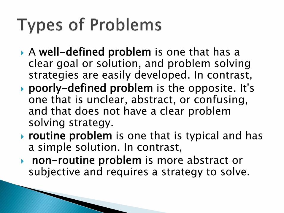
A well-defined problem is one that has a clear goal or solution, and problem solving strategies are easily developed. In contrast,
poorly-defined problem is the opposite. It's one that is unclear, abstract, or confusing, and that does not have a clear problem solving strategy.
routine problem is one that is typical and has a simple solution. In contrast,
non-routine problem is more abstract or subjective and requires a strategy to solve.
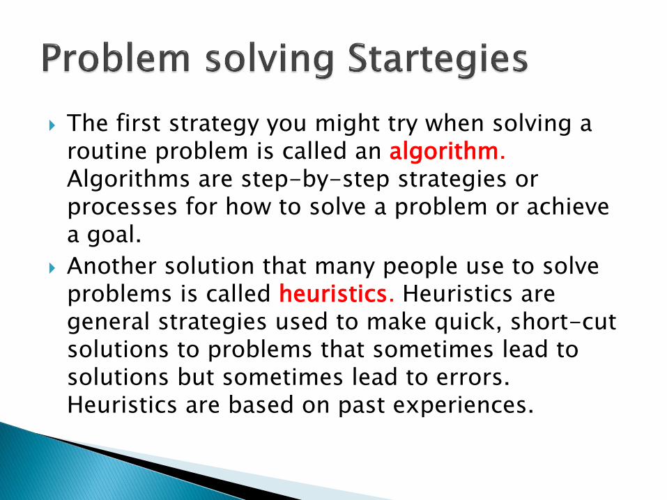
The first strategy you might try when solving a routine problem is called an algorithm. Algorithms are step-by-step strategies or processes for how to solve a problem or achieve a goal.
Another solution that many people use to solve problems is called heuristics. Heuristics are general strategies used to make quick, short-cut solutions to problems that sometimes lead to solutions but sometimes lead to errors. Heuristics are based on past experiences.
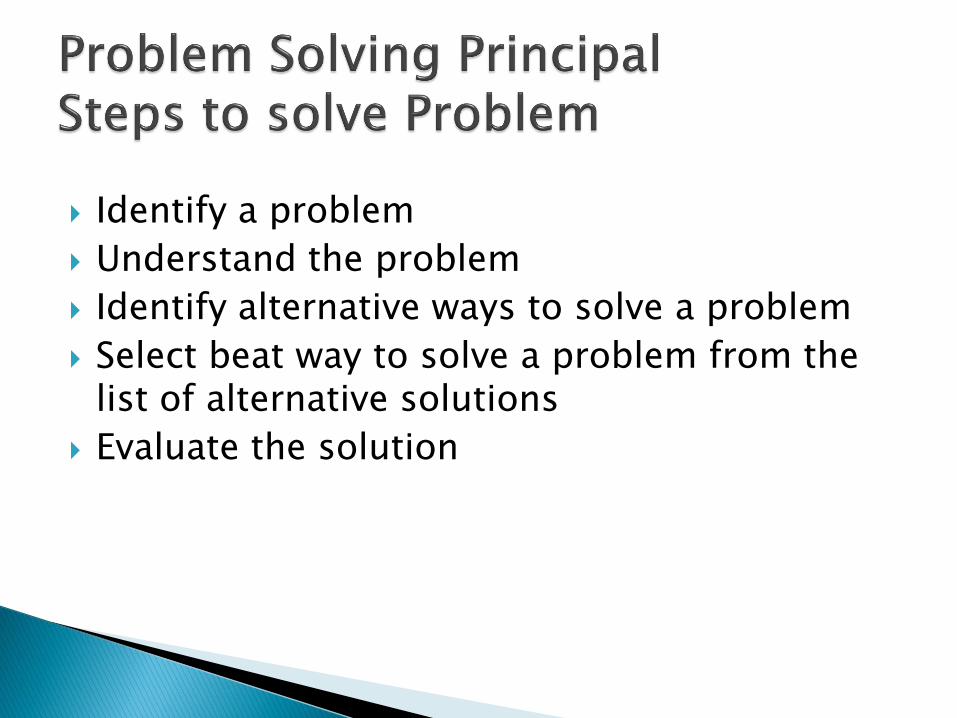
Identify a problem
Understand the problem
Identify alternative ways to solve a problem
Select beat way to solve a problem from the list of alternative solutions
Evaluate the solution
What is an algorithm?
An algorithm is a finite set of precise instructions for performing a computation or for solving a problem.
This is a rather vague definition. You will get to know a more precise and mathematically useful definition when you attend CS420.
But this one is good enough for now…
Fall 2002CMSC 203 - Discrete Structures 8
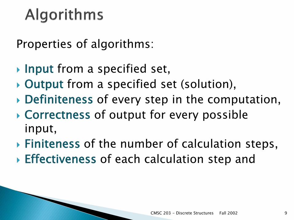
Properties of algorithms:
Input from a specified set,
Output from a specified set (solution),
Definiteness of every step in the computation,
Correctness of output for every possible input,
Finiteness of the number of calculation steps,
Effectiveness of each calculation step and
Fall 2002CMSC 203 - Discrete Structures 9
Why we should analyze algorithms?◦ Predict the resources that the algorithm requires
Computational time (CPU consumption)
Memory space (RAM consumption)
Communication bandwidth consumption
◦ The running time of an algorithm is:
The total number of operations executed
Also known as algorithm complexity
10
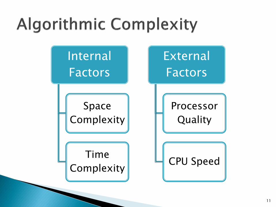
Internal
Factors
Space
Complexity
Time
Complexity
External
Factors
Processor
Quality
CPU Speed
11
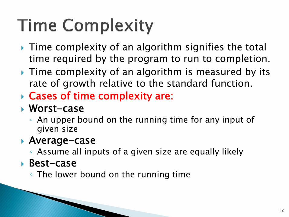
Time complexity of an algorithm signifies the total time required by the program to run to completion.
Time complexity of an algorithm is measured by its rate of growth relative to the standard function.
Cases of time complexity are:
Worst-case◦ An upper bound on the running time for any input of
given size
Average-case◦ Assume all inputs of a given size are equally likely
Best-case◦ The lower bound on the running time
12
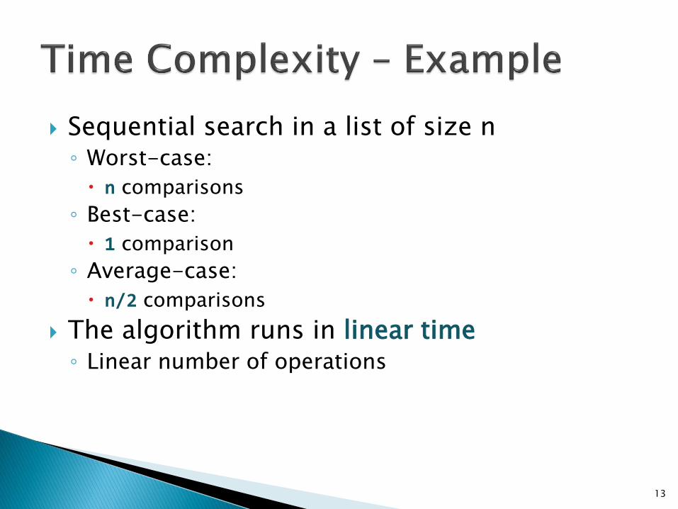
Sequential search in a list of size n◦ Worst-case:
n comparisons
◦ Best-case:
1 comparison
◦ Average-case:
n/2 comparisons
The algorithm runs in linear time◦ Linear number of operations
13
14
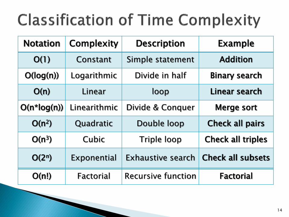
Notation Complexity Description Example
O(1) Constant Simple statement Addition
O(log(n)) Logarithmic Divide in half Binary search
O(n) Linear loop Linear search
O(n*log(n)) Linearithmic Divide & Conquer Merge sort
O(n2) Quadratic Double loop Check all pairs
O(n3) Cubic Triple loop Check all triples
O(2n) Exponential Exhaustive search Check all subsets
O(n!) Factorial Recursive function Factorial
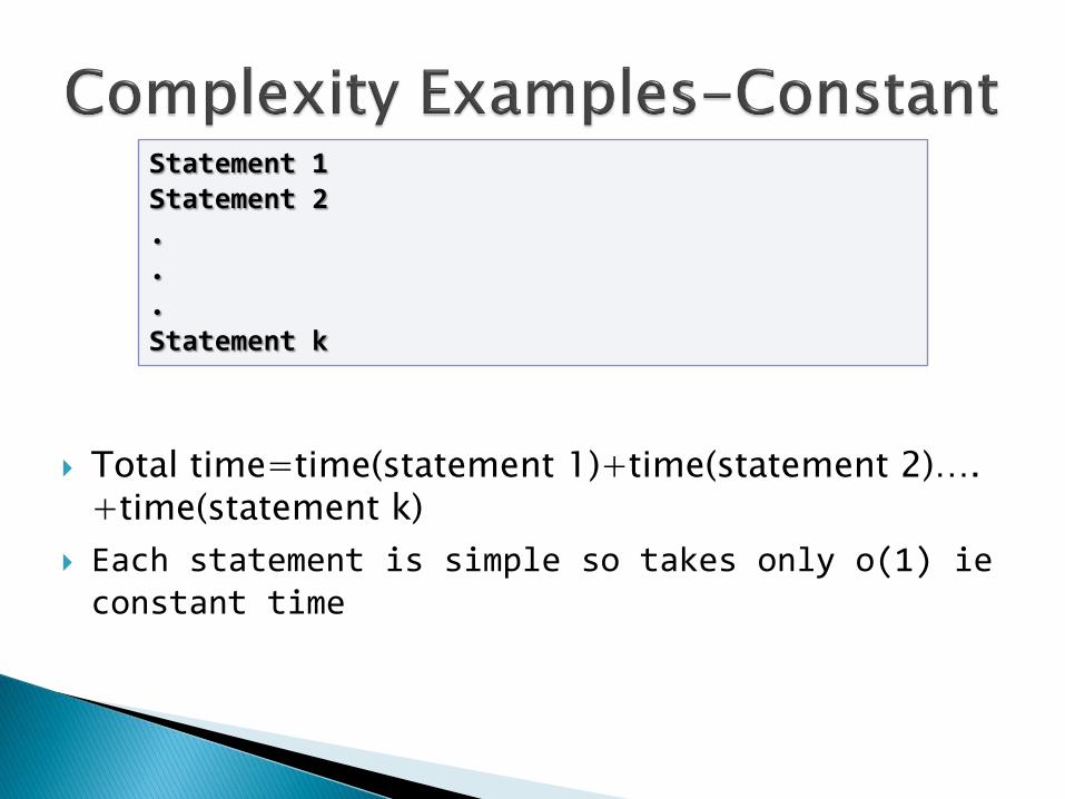
Total time=time(statement 1)+time(statement 2)…. +time(statement k)
Each statement is simple so takes only o(1) ieconstant time
Statement 1Statement 2...Statement k
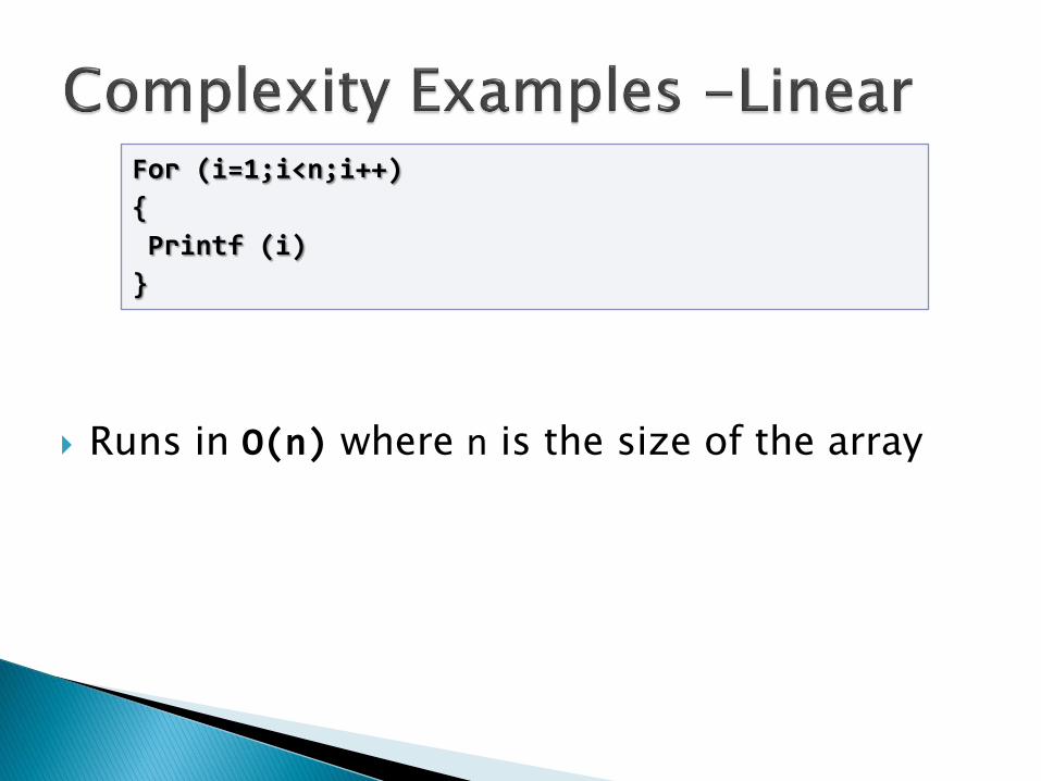
Runs in O(n) where n is the size of the array
For (i=1;i<n;i++)
{
Printf (i)
}
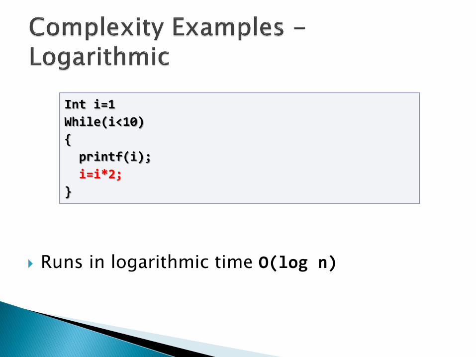
Runs in logarithmic time O(log n)
Int i=1
While(i<10)
{
printf(i);
i=i*2;
}
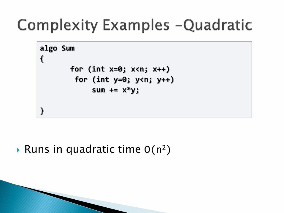
Runs in quadratic time O(n2)
algo Sum
{
for (int x=0; x<n; x++)
for (int y=0; y<n; y++)
sum += x*y;
}
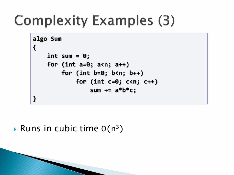
Runs in cubic time O(n3)
algo Sum
{
int sum = 0;
for (int a=0; a<n; a++)
for (int b=0; b<n; b++)
for (int c=0; c<n; c++)
sum += a*b*c;
}
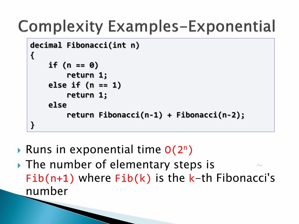
Runs in exponential time O(2n)
The number of elementary steps is ~Fib(n+1) where Fib(k) is the k-th Fibonacci's number
decimal Fibonacci(int n){
if (n == 0)return 1;
else if (n == 1)return 1;
elsereturn Fibonacci(n-1) + Fibonacci(n-2);
}
Running time of an algorithm as a function of input size n.
Expressed using only the highest-order termin the expression for the exact running time.
Describes behavior of function in the limit.
Written using Asymptotic Notation.
Comp 122
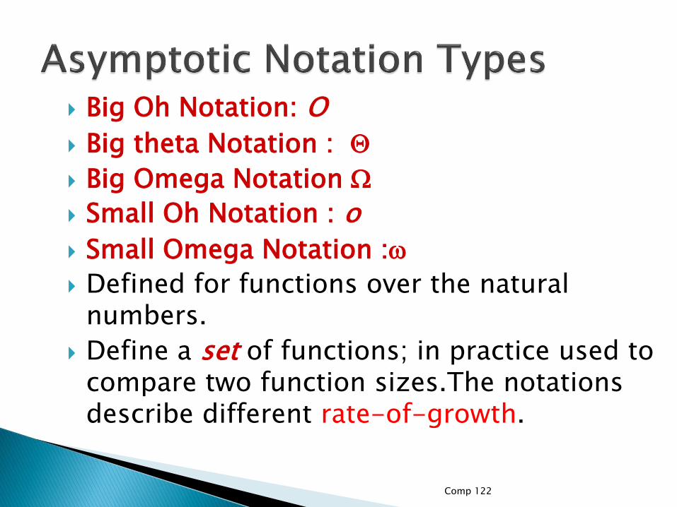
Big Oh Notation: O
Big theta Notation : Q
Big Omega Notation W
Small Oh Notation : o
Small Omega Notation :w
Defined for functions over the natural numbers.
Define a set of functions; in practice used to compare two function sizes.The notations describe different rate-of-growth.
Comp 122
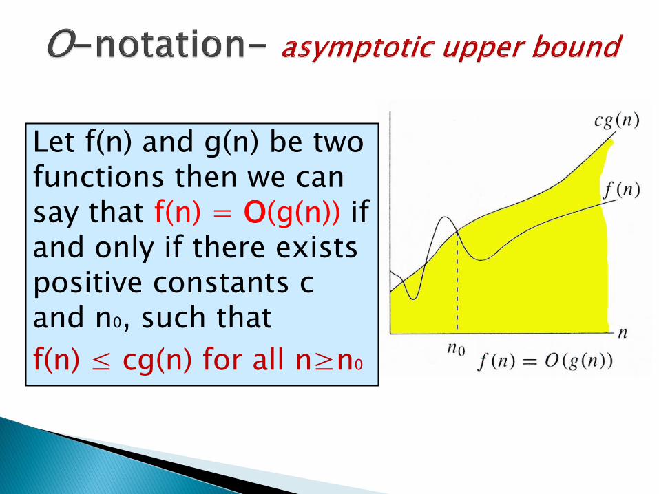
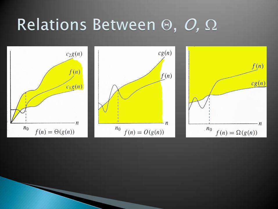
Let f(n) and g(n) be two functions then we can say that f(n) = O(g(n)) if and only if there exists positive constants c and n0, such that
f(n) ≤ cg(n) for all n≥n0
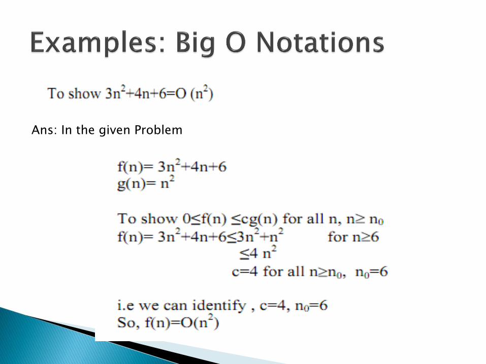
Ans: In the given Problem
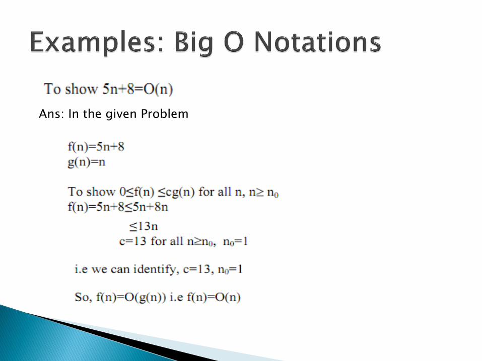
Ans: In the given Problem
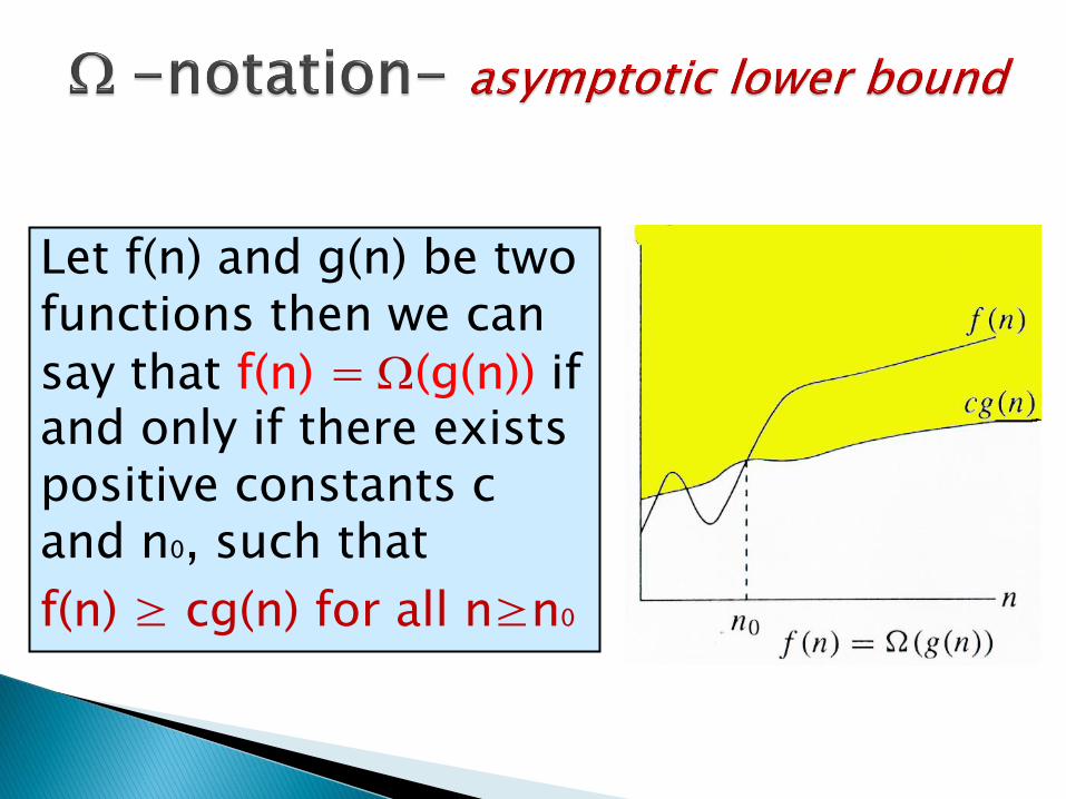
Let f(n) and g(n) be two functions then we can say that f(n) = W(g(n)) if and only if there exists positive constants c and n0, such that
f(n) ≥ cg(n) for all n≥n0
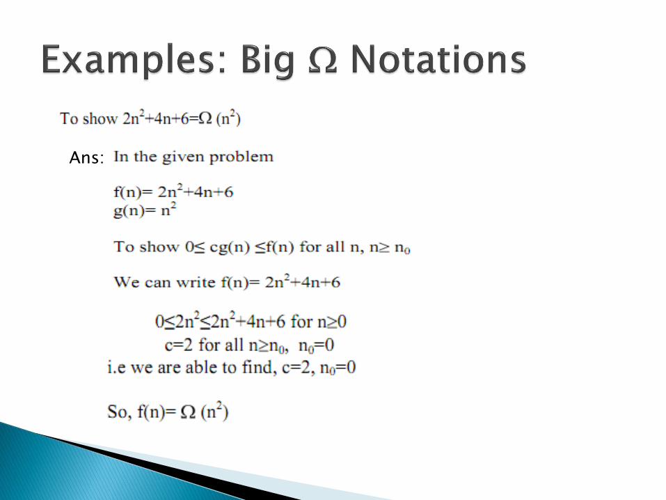
Ans:
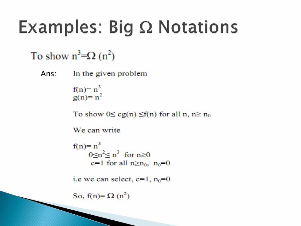
Ans:
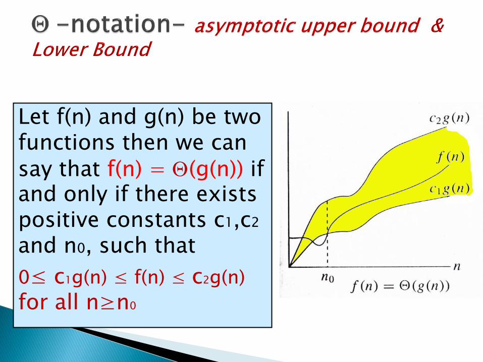
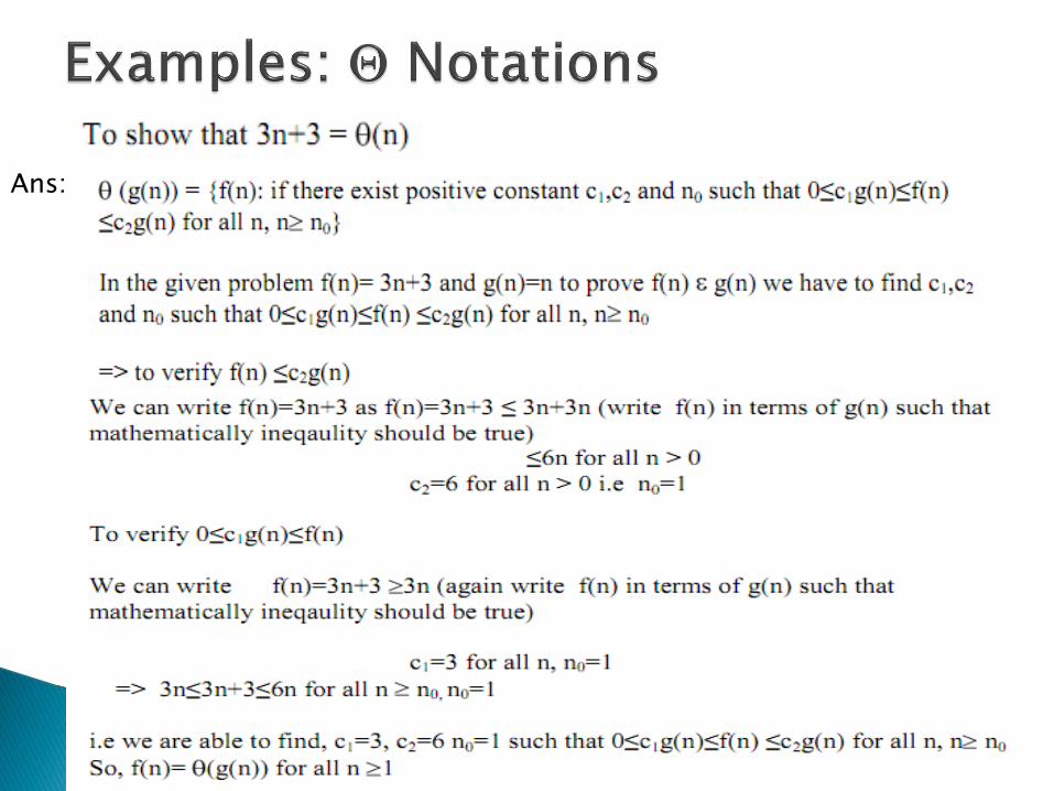
Let f(n) and g(n) be two functions then we can say that f(n) = Q(g(n)) if and only if there exists positive constants c1,c2
and n0, such that
0≤ c1g(n) ≤ f(n) ≤ c2g(n)
for all n≥n0
Ans:
Key point: The time required to perform a sequence of data structure operations is averaged over all operations performed
Amortized analysis can be used to show that◦ The average cost of an operation is small
If one averages over a sequence of operations
even though a single operation might be expensive
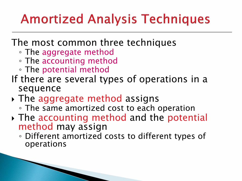
The most common three techniques◦ The aggregate method◦ The accounting method◦ The potential method
If there are several types of operations in a sequence
The aggregate method assigns◦ The same amortized cost to each operation
The accounting method and the potential method may assign◦ Different amortized costs to different types of
operations
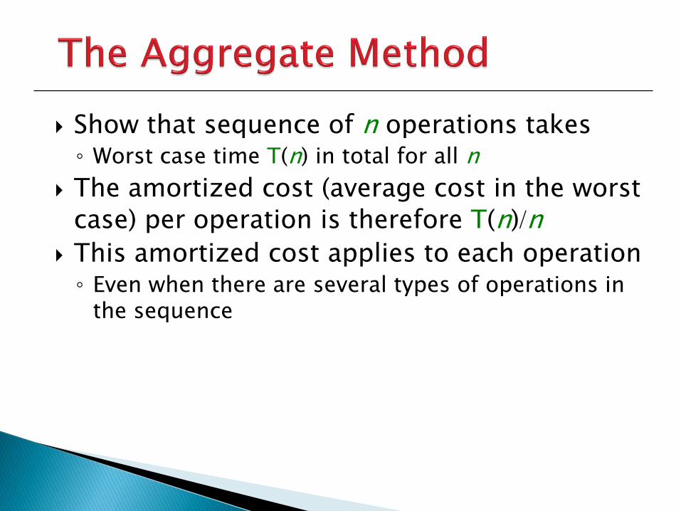
Show that sequence of n operations takes◦ Worst case time T(n) in total for all n
The amortized cost (average cost in the worst
case) per operation is therefore T(n)n
This amortized cost applies to each operation◦ Even when there are several types of operations in
the sequence
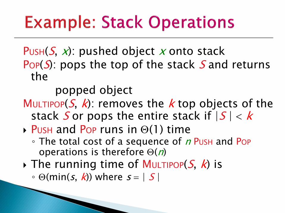
PUSH(S, x): pushed object x onto stackPOP(S): pops the top of the stack S and returns
thepopped object
MULTIPOP(S, k): removes the k top objects of the stack S or pops the entire stack if |S | k
PUSH and POP runs in Q(1) time◦ The total cost of a sequence of n PUSH and POP
operations is therefore Q(n)
The running time of MULTIPOP(S, k) is◦ Q(min(s, k)) where s | S |
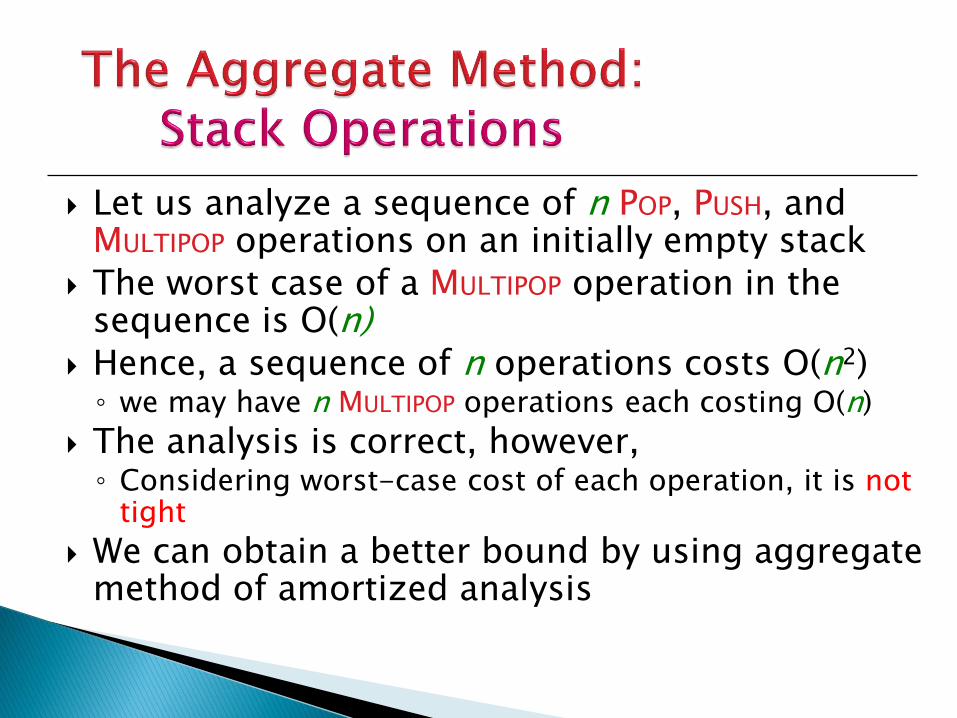
Let us analyze a sequence of n POP, PUSH, and MULTIPOP operations on an initially empty stack
The worst case of a MULTIPOP operation in the sequence is O(n)
Hence, a sequence of n operations costs O(n2)◦ we may have n MULTIPOP operations each costing O(n)
The analysis is correct, however, ◦ Considering worst-case cost of each operation, it is not
tight
We can obtain a better bound by using aggregate method of amortized analysis
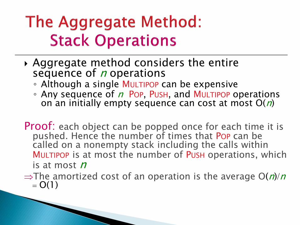
Aggregate method considers the entire sequence of n operations ◦ Although a single MULTIPOP can be expensive◦ Any sequence of n POP, PUSH, and MULTIPOP operations
on an initially empty sequence can cost at most O(n)
Proof: each object can be popped once for each time it is pushed. Hence the number of times that POP can be called on a nonempty stack including the calls within MULTIPOP is at most the number of PUSH operations, which is at most n
The amortized cost of an operation is the average O(n)n O(1)
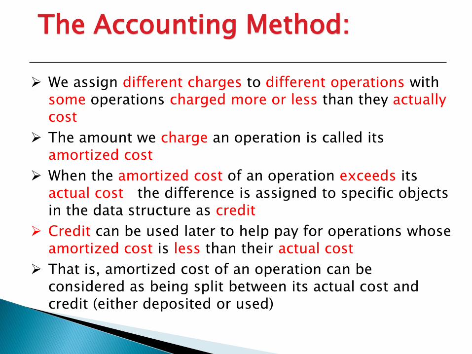
We assign different charges to different operations with some operations charged more or less than they actually cost
The amount we charge an operation is called its amortized cost
When the amortized cost of an operation exceeds its actual cost the difference is assigned to specific objects in the data structure as credit
Credit can be used later to help pay for operations whose amortized cost is less than their actual cost
That is, amortized cost of an operation can be considered as being split between its actual cost and credit (either deposited or used)
The Accounting Method:
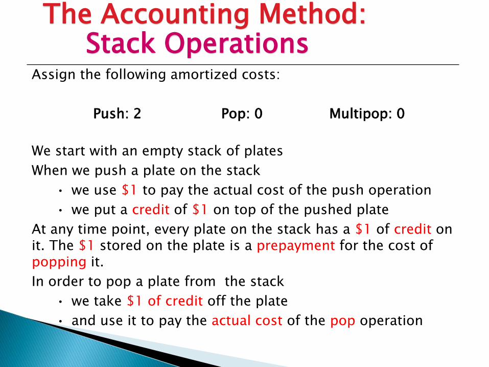
Assign the following amortized costs:
Push: 2 Pop: 0 Multipop: 0
We start with an empty stack of plates
When we push a plate on the stack
• we use $1 to pay the actual cost of the push operation
• we put a credit of $1 on top of the pushed plate
At any time point, every plate on the stack has a $1 of credit on it. The $1 stored on the plate is a prepayment for the cost of popping it.
In order to pop a plate from the stack
• we take $1 of credit off the plate
• and use it to pay the actual cost of the pop operation
The Accounting Method:Stack Operations
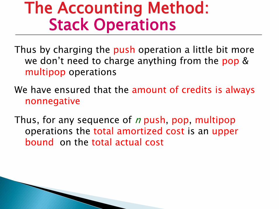
Thus by charging the push operation a little bit more we don’t need to charge anything from the pop & multipop operations
We have ensured that the amount of credits is always nonnegative
Thus, for any sequence of n push, pop, multipopoperations the total amortized cost is an upper bound on the total actual cost
The Accounting Method:Stack Operations
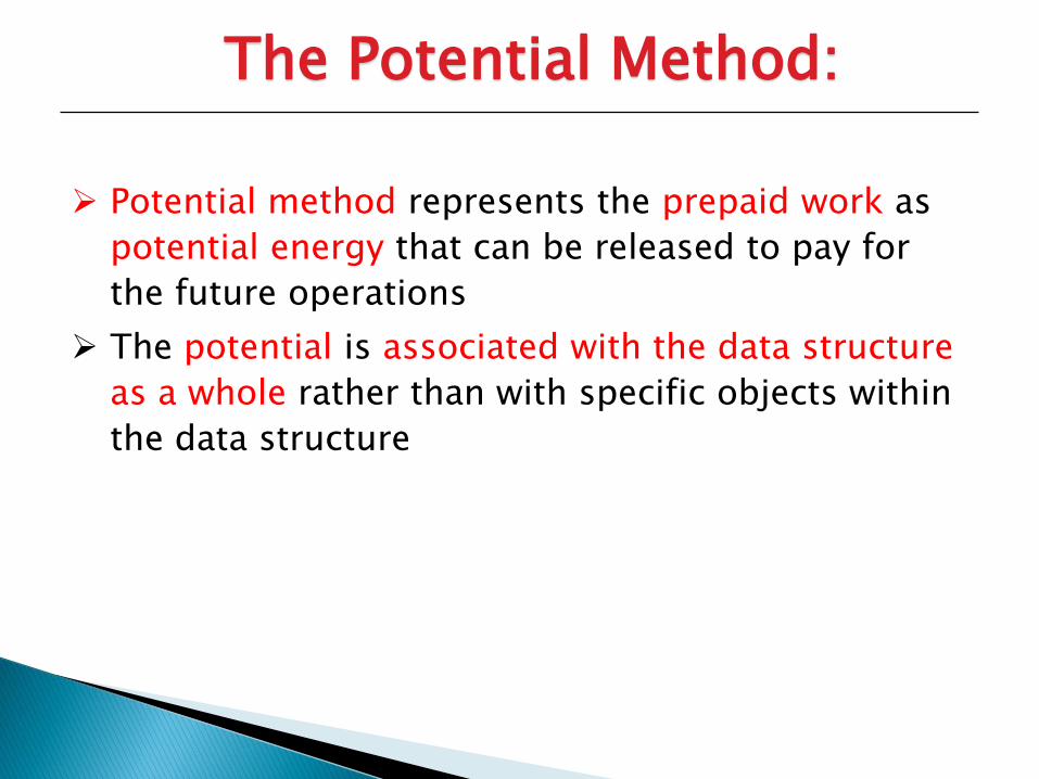
Potential method represents the prepaid work as
potential energy that can be released to pay for
the future operations
The potential is associated with the data structure
as a whole rather than with specific objects within
the data structure
The Potential Method:
The Potential Method
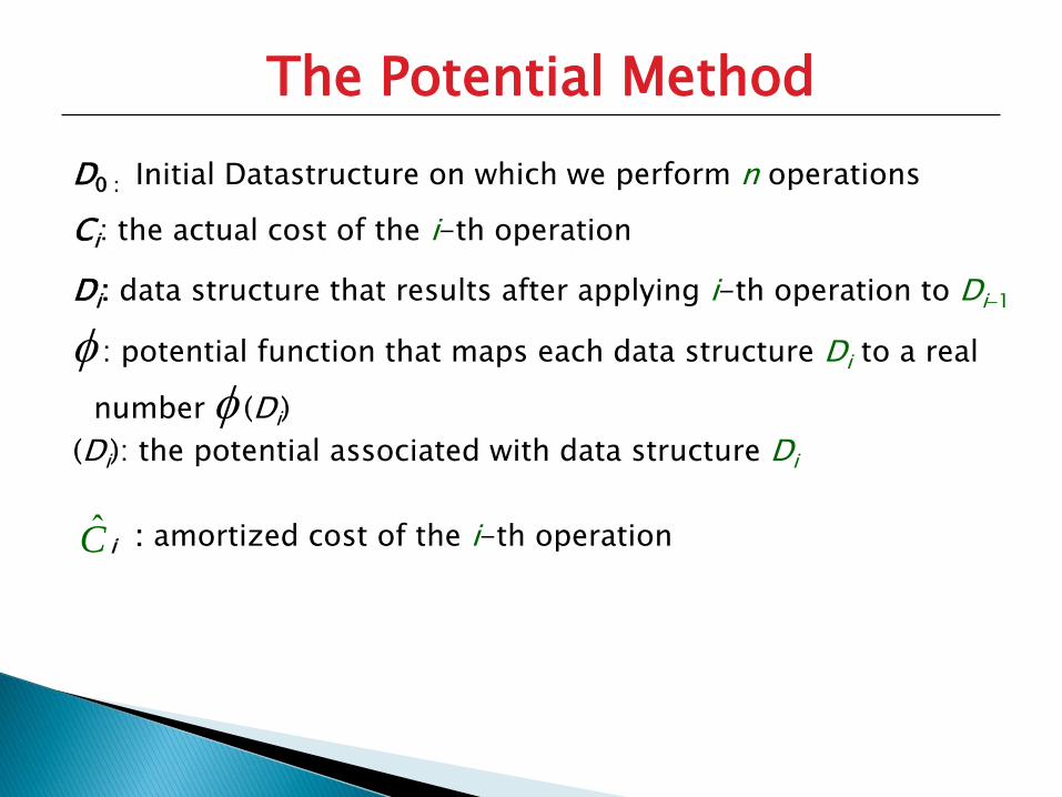
D0 : Initial Datastructure on which we perform n operations
Ci: the actual cost of the i-th operation
Di: data structure that results after applying i-th operation to Di1
: potential function that maps each data structure Di to a real
number (Di)
(Di): the potential associated with data structure Di
i : amortized cost of the i-th operation C
The Potential Method
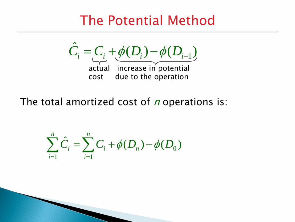
actual increase in potentialcost due to the operation
The total amortized cost of n operations is:
)()(ˆ1 iiii DDCC
n
i
ni
n
i
i DDCC1
0
1
)()( ˆ
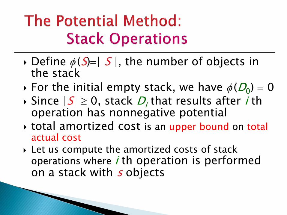
Define (S)| S |, the number of objects in the stack
For the initial empty stack, we have (D0) 0 Since |S| 0, stack Di that results after i th
operation has nonnegative potential total amortized cost is an upper bound on total
actual cost
Let us compute the amortized costs of stack operations where i th operation is performed on a stack with s objects
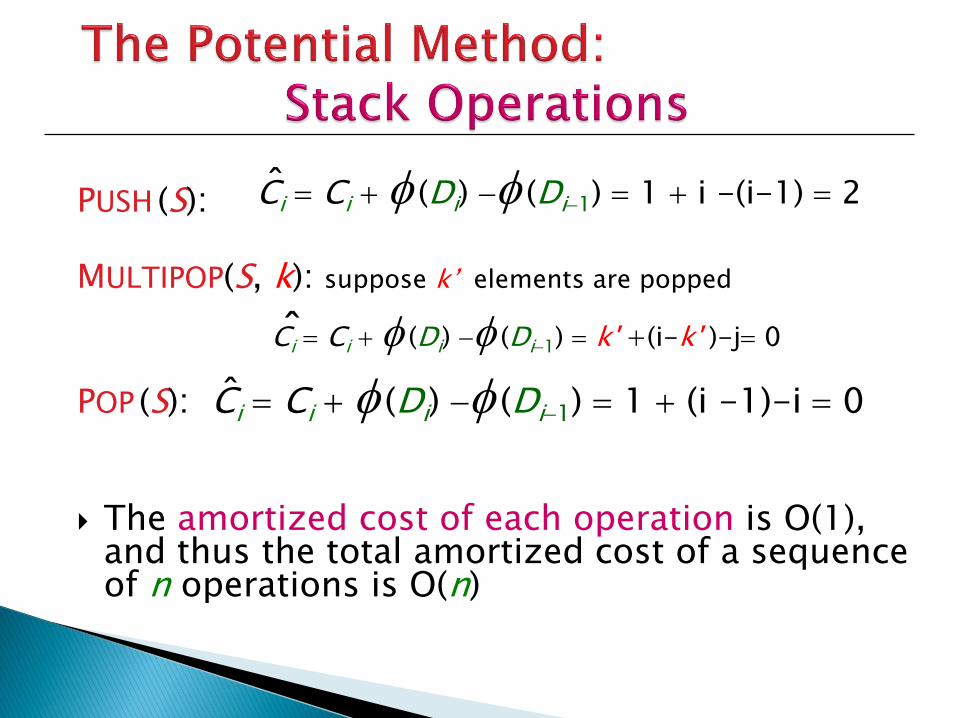
PUSH (S):
MULTIPOP(S, k): suppose k’ elements are popped
POP (S): Ci Ci (Di) (Di1) 1 (i -1)-i 0
The amortized cost of each operation is O(1), and thus the total amortized cost of a sequence of n operations is O(n)
Ci Ci (Di) (Di1) 1 i -(i-1) 2ˆ
Ci Ci (Di) (Di1) k' +(i-k' )-j 0ˆ
ˆ
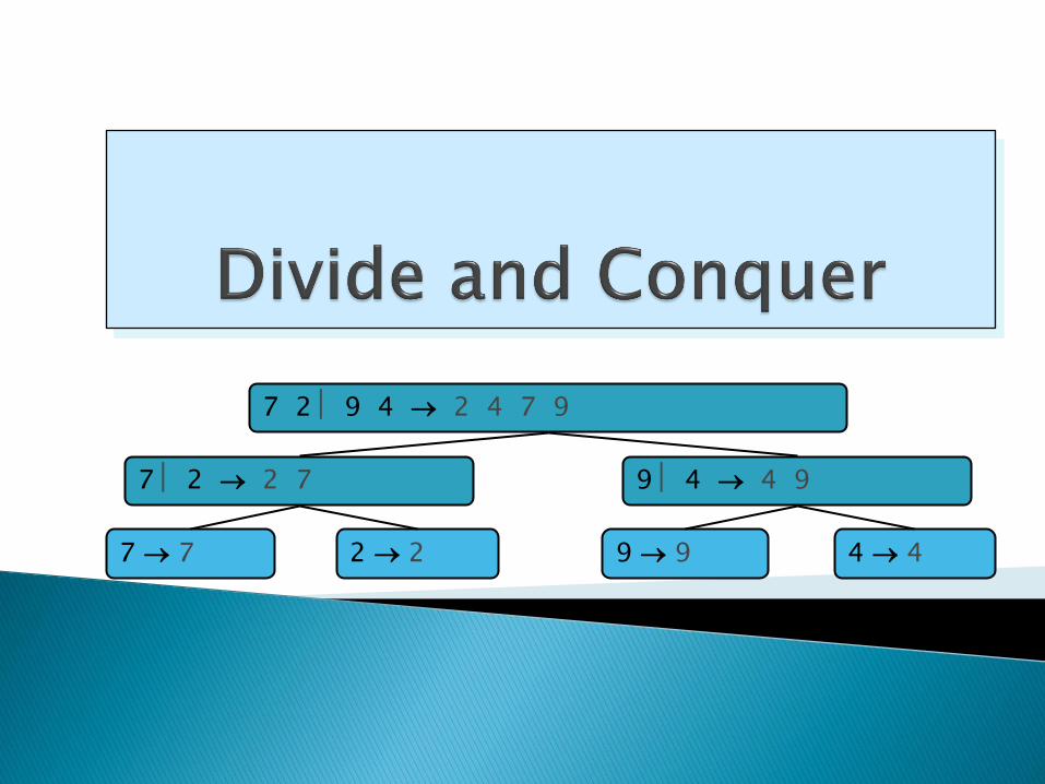
7 2 9 4 2 4 7 9
7 2 2 7 9 4 4 9
7 7 2 2 9 9 4 4
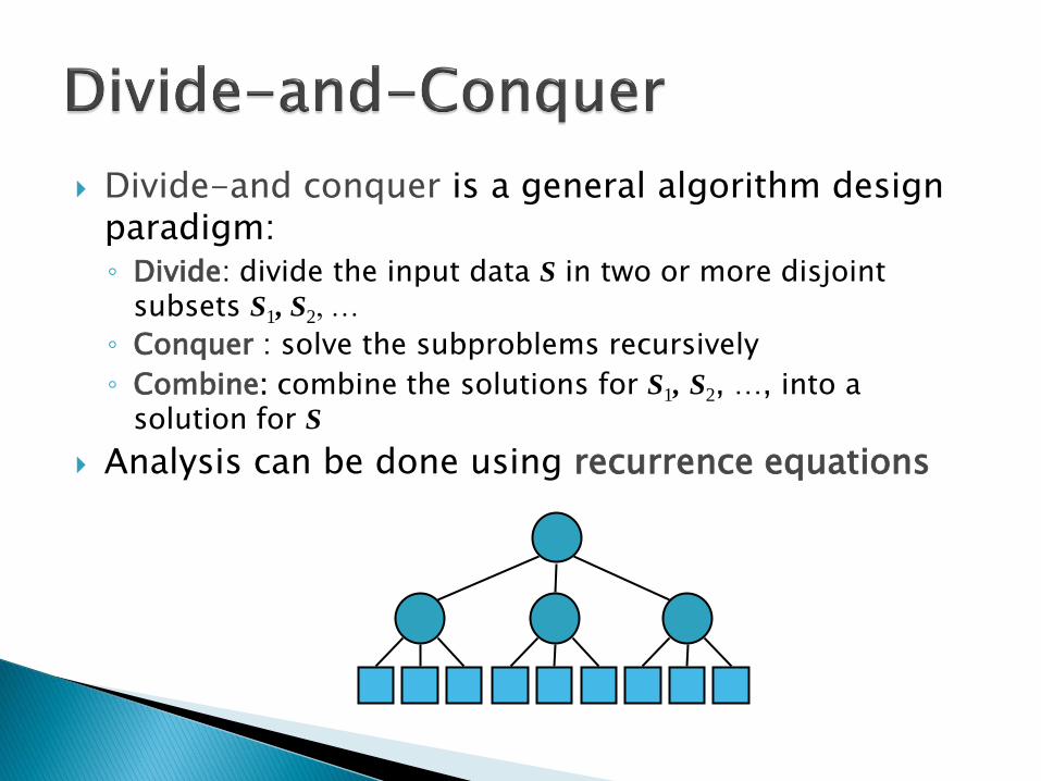
Divide-and conquer is a general algorithm design paradigm:◦ Divide: divide the input data S in two or more disjoint
subsets S1, S2, …
◦ Conquer : solve the subproblems recursively
◦ Combine: combine the solutions for S1, S2, …, into a solution for S
Analysis can be done using recurrence equations
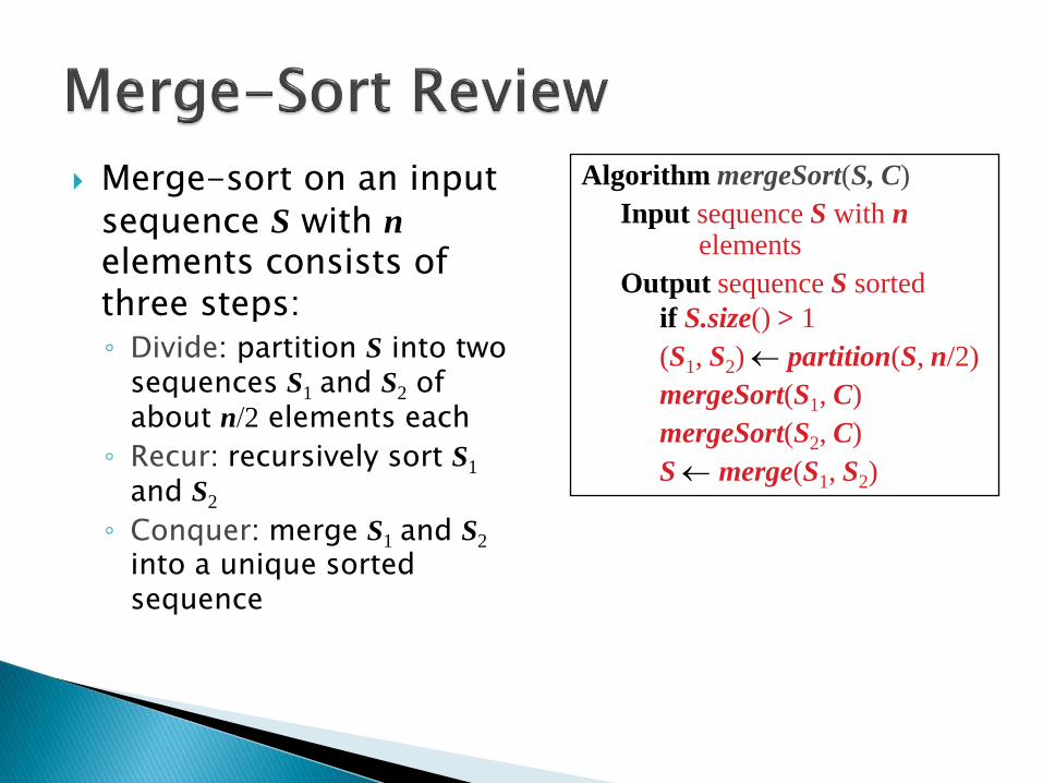
Merge-sort on an input sequence S with nelements consists of three steps:◦ Divide: partition S into two
sequences S1 and S2 of about n2 elements each
◦ Recur: recursively sort S1
and S2
◦ Conquer: merge S1 and S2
into a unique sorted sequence
Algorithm mergeSort(S, C)
Input sequence S with nelements
Output sequence S sorted
if S.size() > 1
(S1, S2) partition(S, n/2)
mergeSort(S1, C)
mergeSort(S2, C)
S merge(S1, S2)
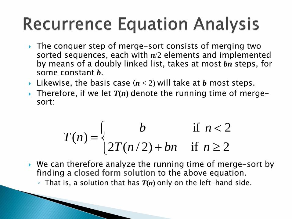
The conquer step of merge-sort consists of merging two sorted sequences, each with n2 elements and implemented by means of a doubly linked list, takes at most bn steps, for some constant b.
Likewise, the basis case (n < 2) will take at b most steps.
Therefore, if we let T(n) denote the running time of merge-sort:
We can therefore analyze the running time of merge-sort by finding a closed form solution to the above equation.◦ That is, a solution that has T(n) only on the left-hand side.
2if)2/(2
2if )(
nbnnT
nbnT
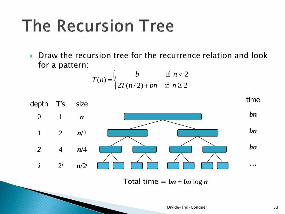
Draw the recursion tree for the recurrence relation and look for a pattern:
Divide-and-Conquer 53
depth T’s size
0 1 n
1 2 n2
2 4 n4
i 2i n2i
2if)2/(2
2if )(
nbnnT
nbnT
time
bn
bn
bn
…
Total time = bn + bn log n
19 June 2015Comp 122, Spring 2004
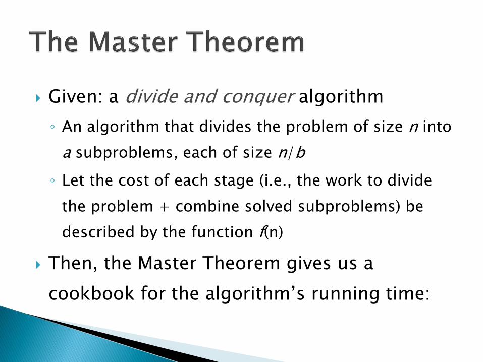
Given: a divide and conquer algorithm
◦ An algorithm that divides the problem of size n into
a subproblems, each of size n/b
◦ Let the cost of each stage (i.e., the work to divide
the problem + combine solved subproblems) be
described by the function f(n)
Then, the Master Theorem gives us a
cookbook for the algorithm’s running time:
Divide-and-Conquer 56
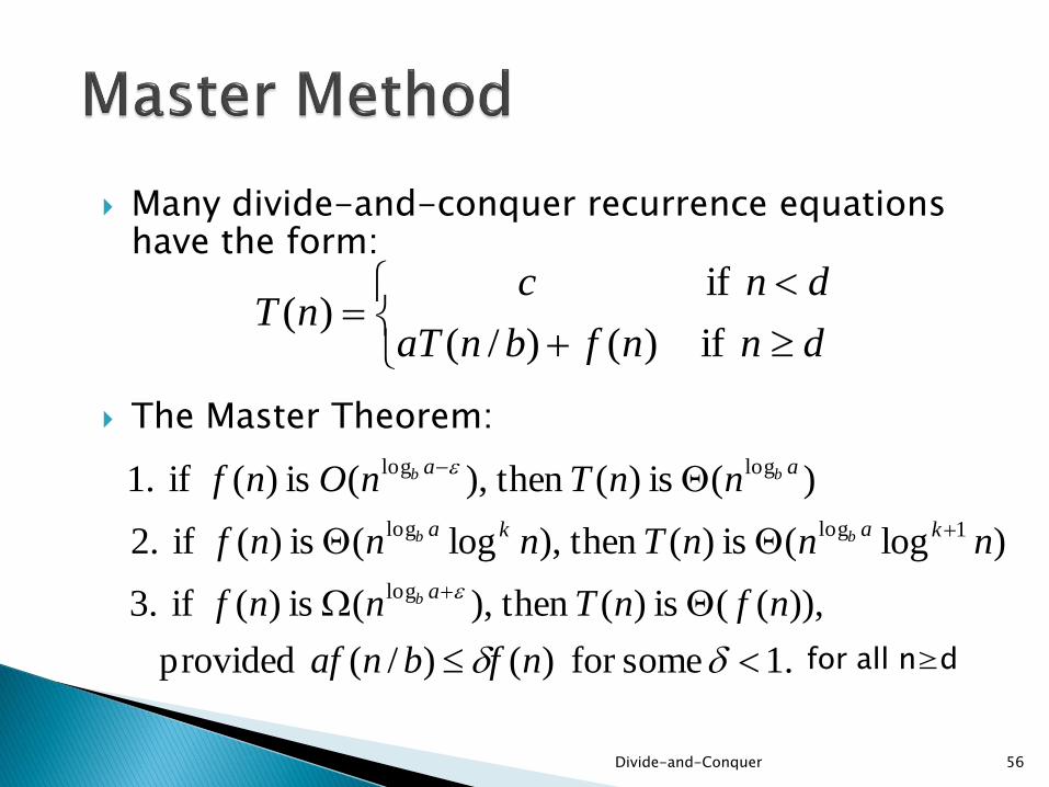
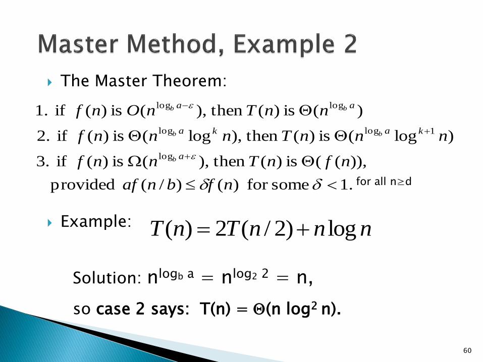
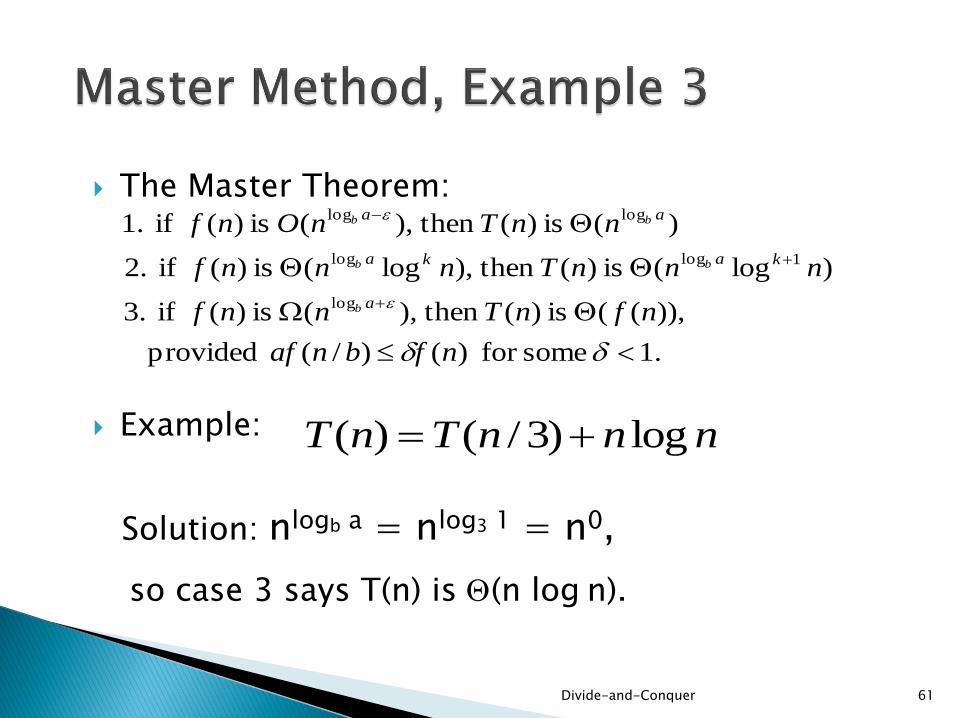
Many divide-and-conquer recurrence equations have the form:
The Master Theorem:
dnnfbnaT
dncnT
if)()/(
if )(
.1 somefor )()/( provided
)),((is)(then),(is)(if 3.
)log(is)(then),log(is)(if 2.
)(is)(then),(is)(if 1.
log
1loglog
loglog
QW
Q
nfbnaf
nfnTnnf
nnnTnnnf
nnTnOnf
a
kaka
aa
b
bb
bb
for all n≥d
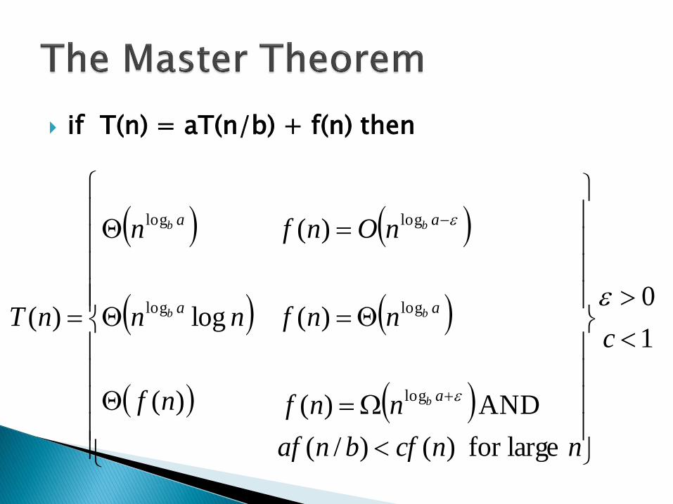
if T(n) = aT(n/b) + f(n) then
W
Q
Q
Q
Q
1
0
largefor )()/(
AND )(
)(
)(
)(
log)(
log
log
log
log
log
c
nncfbnaf
nnf
nnf
nOnf
nf
nn
n
nT
a
a
a
a
a
b
b
b
b
b
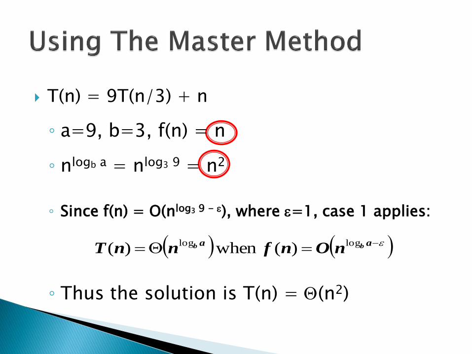
T(n) = 9T(n/3) + n
◦ a=9, b=3, f(n) = n
◦ nlogb a = nlog3 9 = n2
◦ Since f(n) = O(nlog3 9 - ), where =1, case 1 applies:
◦ Thus the solution is T(n) = Q(n2)
Qaa bb nOnfnnT
loglog)( when )(
The Master Theorem:
Example:
Divide-and-Conquer 59
.1 somefor )()/( provided
)),((is)(then),(is)(if 3.
)log(is)(then),log(is)(if 2.
)(is)(then),(is)(if 1.
log
1loglog
loglog
QW
Q
nfbnaf
nfnTnnf
nnnTnnnf
nnTnOnf
ab
kakab
aab
b
b
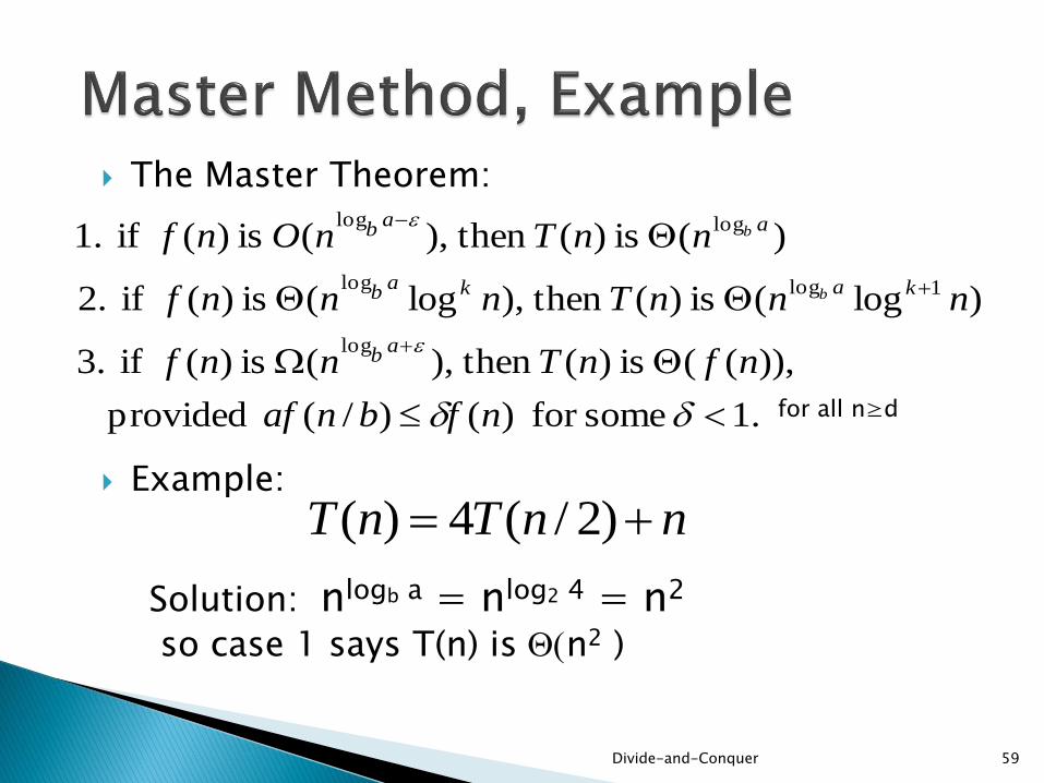
nnTnT )2/(4)(
Solution: nlogb a = nlog2 4 = n2
so case 1 says T(n) is Qn2 )
for all n≥d
The Master Theorem:
Example:
60
.1 somefor )()/( provided
)),((is)(then),(is)(if 3.
)log(is)(then),log(is)(if 2.
)(is)(then),(is)(if 1.
log
1loglog
loglog
QW
Q
nfbnaf
nfnTnnf
nnnTnnnf
nnTnOnf
a
kaka
aa
b
bb
bb
nnnTnT log)2/(2)(
Solution: nlogb a = nlog2 2 = n,
so case 2 says: T(n) = Q(n log2 n).
for all n≥d
The Master Theorem:
Example:
Divide-and-Conquer 61
.1 somefor )()/( provided
)),((is)(then),(is)(if 3.
)log(is)(then),log(is)(if 2.
)(is)(then),(is)(if 1.
log
1loglog
loglog
QW
Q
nfbnaf
nfnTnnf
nnnTnnnf
nnTnOnf
a
kaka
aa
b
bb
bb
nnnTnT log)3/()(
Solution: nlogb a = nlog3 1 = n0,
so case 3 says T(n) is Q(n log n).
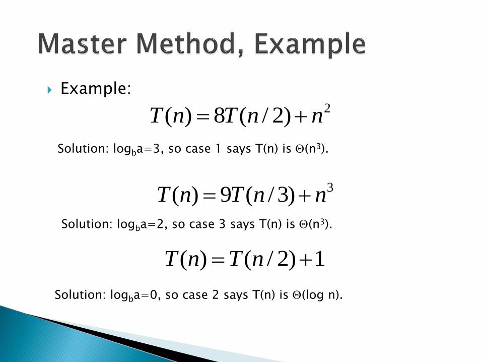
Example:2)2/(8)( nnTnT
Solution: logba=3, so case 1 says T(n) is Q(n3).
3)3/(9)( nnTnT
Solution: logba=2, so case 3 says T(n) is Q(n3).
1)2/()( nTnT
Solution: logba=0, so case 2 says T(n) is Q(log n).