Embed Size (px)
Citation preview

Data Base and Data Mining Group of Politecnico di Torino
DBMG
Classification fundamentals
Elena BaralisPolitecnico di Torino

2DBMG
Classification
◼ Objectives
◼ prediction of a class label
◼ definition of an interpretable model of a given phenomenon
model
training data
unclassified data classified data

5DBMG
Classification
◼ Applications◼ detection of customer propension to leave a company
(churn or attrition)◼ fraud detection◼ classification of different pathology types◼ …
model
training data
unclassified data classified data

6DBMG
Classification: definition
◼ Given
◼ a collection of class labels
◼ a collection of data objects labelled with a class label
◼ Find a descriptive profile of each class, which will allow the assignment of unlabeled objects to the appropriate class

7DBMG
Definitions
◼ Training set
◼ Collection of labeled data objects used to learn the classification model
◼ Test set
◼ Collection of labeled data objects used to validate the classification model

8DBMG
Classification techniques
◼ Decision trees
◼ Classification rules
◼ Association rules
◼ Neural Networks
◼ Naïve Bayes and Bayesian Networks
◼ k-Nearest Neighbours (k-NN)
◼ Support Vector Machines (SVM)
◼ …
9DBMG
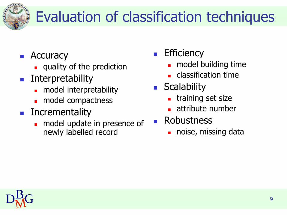
◼ Accuracy◼ quality of the prediction
◼ Interpretability◼ model interpretability
◼ model compactness
◼ Incrementality◼ model update in presence of
newly labelled record
Evaluation of classification techniques
◼ Efficiency◼ model building time
◼ classification time
◼ Scalability◼ training set size
◼ attribute number
◼ Robustness◼ noise, missing data

Data Base and Data Mining Group of Politecnico di Torino
DBMG
Decision trees
Elena BaralisPolitecnico di Torino

11DBMG
Example of decision tree
Tid Refund MaritalStatus
TaxableIncome Cheat
1 Yes Single 125K No
2 No Married 100K No
3 No Single 70K No
4 Yes Married 120K No
5 No Divorced 95K Yes
6 No Married 60K No
7 Yes Divorced 220K No
8 No Single 85K Yes
9 No Married 75K No
10 No Single 90K Yes10
Refund
MarSt
TaxInc
YESNO
NO
NO
Yes No
MarriedSingle, Divorced
< 80K > 80K
Splitting Attributes
Training Data Model: Decision Tree
From: Tan,Steinbach, Kumar, Introduction to Data Mining, McGraw Hill 2006

12DBMG
Another example of decision tree
Tid Refund MaritalStatus
TaxableIncome Cheat
1 Yes Single 125K No
2 No Married 100K No
3 No Single 70K No
4 Yes Married 120K No
5 No Divorced 95K Yes
6 No Married 60K No
7 Yes Divorced 220K No
8 No Single 85K Yes
9 No Married 75K No
10 No Single 90K Yes10
MarSt
Refund
TaxInc
YESNO
NO
NO
Yes No
MarriedSingle,
Divorced
< 80K > 80K
There could be more than one tree that fits the same data!
From: Tan,Steinbach, Kumar, Introduction to Data Mining, McGraw Hill 2006

13DBMG
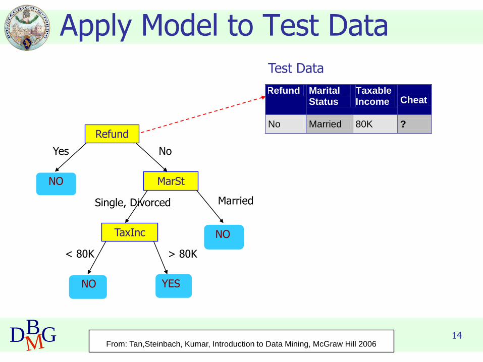
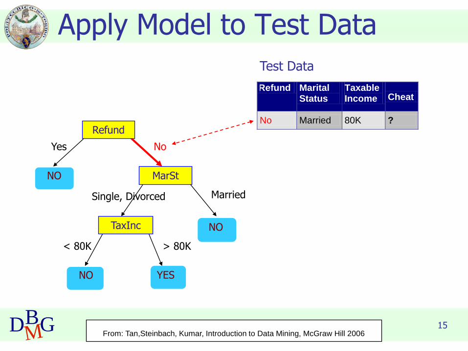
Apply Model to Test Data
Refund
MarSt
TaxInc
YESNO
NO
NO
Yes No
MarriedSingle, Divorced
< 80K > 80K
Refund Marital Status
Taxable Income Cheat
No Married 80K ? 10
Test DataStart from the root of tree.
From: Tan,Steinbach, Kumar, Introduction to Data Mining, McGraw Hill 2006
14DBMG
Apply Model to Test Data
Refund
MarSt
TaxInc
YESNO
NO
NO
Yes No
MarriedSingle, Divorced
< 80K > 80K
Refund Marital Status
Taxable Income Cheat
No Married 80K ? 10
Test Data
From: Tan,Steinbach, Kumar, Introduction to Data Mining, McGraw Hill 2006
15DBMG
Apply Model to Test Data
Refund
MarSt
TaxInc
YESNO
NO
NO
Yes No
MarriedSingle, Divorced
< 80K > 80K
Refund Marital Status
Taxable Income Cheat
No Married 80K ? 10
Test Data
From: Tan,Steinbach, Kumar, Introduction to Data Mining, McGraw Hill 2006

16DBMG
Apply Model to Test Data
Refund
MarSt
TaxInc
YESNO
NO
NO
Yes No
MarriedSingle, Divorced
< 80K > 80K
Refund Marital Status
Taxable Income Cheat
No Married 80K ? 10
Test Data
From: Tan,Steinbach, Kumar, Introduction to Data Mining, McGraw Hill 2006

17DBMG
Apply Model to Test Data
Refund
MarSt
TaxInc
YESNO
NO
NO
Yes No
Married Single, Divorced
< 80K > 80K
Refund Marital Status
Taxable Income Cheat
No Married 80K ? 10
Test Data
From: Tan,Steinbach, Kumar, Introduction to Data Mining, McGraw Hill 2006

18DBMG
Apply Model to Test Data
Refund
MarSt
TaxInc
YESNO
NO
NO
Yes No
Married Single, Divorced
< 80K > 80K
Refund Marital Status
Taxable Income Cheat
No Married 80K ? 10
Test Data
Assign Cheat to “No”
From: Tan,Steinbach, Kumar, Introduction to Data Mining, McGraw Hill 2006
19DBMG
Decision tree induction
◼ Many algorithms to build a decision tree
◼ Hunt’s Algorithm (one of the earliest)
◼ CART
◼ ID3, C4.5, C5.0
◼ SLIQ, SPRINT
From: Tan,Steinbach, Kumar, Introduction to Data Mining, McGraw Hill 2006

20DBMG
General structure of Hunt’s algorithm
Basic steps
◼ If Dt contains records that belong to more than one class◼ select the “best” attribute A on which
to split Dt and label node t as A
◼ split Dt into smaller subsets and recursively apply the procedure to each subset
◼ If Dt contains records that belong to the same class yt
◼ then t is a leaf node labeled as yt
◼ If Dt is an empty set◼ then t is a leaf node labeled as the
default (majority) class, yd
Dt
t
From: Tan,Steinbach, Kumar, Introduction to Data Mining, McGraw Hill 2006
Dt,, set of training records that reach a node t
Tid Refund Marital Status
Taxable Income Cheat
1 Yes Single 125K No
2 No Married 100K No
3 No Single 70K No
4 Yes Married 120K No
5 No Divorced 95K Yes
6 No Married 60K No
7 Yes Divorced 220K No
8 No Single 85K Yes
9 No Married 75K No
10 No Single 90K Yes 10

21DBMG
Hunt’s algorithm
Don’t
Cheat
Refund
Don’t
Cheat
Don’t
Cheat
Yes No
Refund
Don’t
Cheat
Yes No
Marital
Status
Don’t
Cheat
Cheat
Single,Divorced
Married
Taxable
Income
Don’t
Cheat
< 80K >= 80K
Refund
Don’t
Cheat
Yes No
Marital
Status
Don’t
CheatCheat
Single,Divorced
Married
Tid Refund MaritalStatus
TaxableIncome Cheat
1 Yes Single 125K No
2 No Married 100K No
3 No Single 70K No
4 Yes Married 120K No
5 No Divorced 95K Yes
6 No Married 60K No
7 Yes Divorced 220K No
8 No Single 85K Yes
9 No Married 75K No
10 No Single 90K Yes10
From: Tan,Steinbach, Kumar, Introduction to Data Mining, McGraw Hill 2006

22DBMG
Decision tree induction
◼ Adopts a greedy strategy
◼ “Best” attribute for the split is selected locally at each step
◼ not a global optimum
◼ Issues
◼ Structure of test condition
◼ Binary split versus multiway split
◼ Selection of the best attribute for the split
◼ Stopping condition for the algorithm

23DBMG
Structure of test condition
◼ Depends on attribute type
◼ nominal
◼ ordinal
◼ continuous
◼ Depends on number of outgoing edges
◼ 2-way split
◼ multi-way split
From: Tan,Steinbach, Kumar, Introduction to Data Mining, McGraw Hill 2006

24DBMG
Splitting on nominal attributes
◼ Multi-way split
◼ use as many partitions as distinct values
◼ Binary split
◼ Divides values into two subsets
◼ Need to find optimal partitioning
CarTypeFamily
Sports
Luxury
CarType{Family, Luxury} {Sports}
CarType{Sports, Luxury} {Family} OR
From: Tan,Steinbach, Kumar, Introduction to Data Mining, McGraw Hill 2006

25DBMG
◼ Multi-way split
◼ use as many partitions as distinct values
◼ Binary split
◼ Divides values into two subsets
◼ Need to find optimal partitioning
What about this split?
Splitting on ordinal attributes
SizeSmall
Medium
Large
Size{Medium,
Large} {Small}
Size{Small,
Medium} {Large}
OR
Size{Small, Large} {Medium}
From: Tan,Steinbach, Kumar, Introduction to Data Mining, McGraw Hill 2006
26DBMG
Splitting on continuous attributes
◼ Different techniques
◼ Discretization to form an ordinal categorical attribute
◼ Static – discretize once at the beginning
◼ Dynamic – discretize during tree induction
Ranges can be found by equal interval bucketing, equal frequency bucketing (percentiles), or clustering
◼ Binary decision (A < v) or (A v)
◼ consider all possible splits and find the best cut
◼ more computationally intensive
From: Tan,Steinbach, Kumar, Introduction to Data Mining, McGraw Hill 2006

27DBMG
Splitting on continuous attributes
Taxable
Income
> 80K?
Yes No
Taxable
Income?
(i) Binary split (ii) Multi-way split
< 10K
[10K,25K) [25K,50K) [50K,80K)
> 80K
From: Tan,Steinbach, Kumar, Introduction to Data Mining, McGraw Hill 2006

28DBMG
Selection of the best attribute
Own
Car?
C0: 6
C1: 4
C0: 4
C1: 6
C0: 1
C1: 3
C0: 8
C1: 0
C0: 1
C1: 7
Car
Type?
C0: 1
C1: 0
C0: 1
C1: 0
C0: 0
C1: 1
Student
ID?
...
Yes No Family
Sports
Luxury c1
c10
c20
C0: 0
C1: 1...
c11
Before splitting: 10 records of class 0,10 records of class 1
Which attribute (test condition) is the best?
From: Tan,Steinbach, Kumar, Introduction to Data Mining, McGraw Hill 2006

29DBMG
◼ Attributes with homogeneous class distribution are preferred
◼ Need a measure of node impurity
C0: 5
C1: 5
C0: 9
C1: 1
Non-homogeneous, high degree of impurity
Homogeneous, low degree of impurity
From: Tan,Steinbach, Kumar, Introduction to Data Mining, McGraw Hill 2006
Selection of the best attribute

30DBMG
Measures of node impurity
◼ Many different measures available
◼ Gini index
◼ Entropy
◼ Misclassification error
◼ Different algorithms rely on different measures
From: Tan,Steinbach, Kumar, Introduction to Data Mining, McGraw Hill 2006

31DBMG
How to find the best attribute
Before Splitting:
A?
Yes No
Node N1 Node N2
C0 N10
C1 N11
C0 N20
C1 N21
B?
Yes No
Node N3 Node N4
C0 N30
C1 N31
C0 N40
C1 N41
C0 N00
C1 N01
M0
M1 M2 M3 M4
M12 M34Gain = M0 – M12 vs M0 – M34
From: Tan,Steinbach, Kumar, Introduction to Data Mining, McGraw Hill 2006
32DBMG
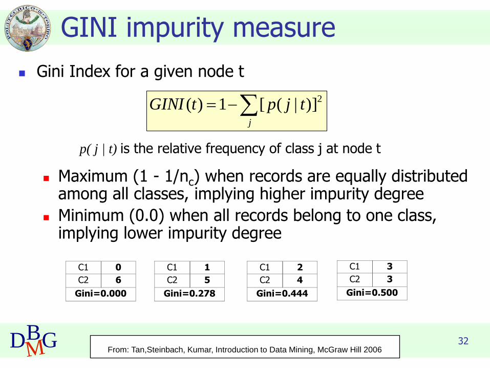
GINI impurity measure
◼ Gini Index for a given node t
p( j | t) is the relative frequency of class j at node t
◼ Maximum (1 - 1/nc) when records are equally distributed among all classes, implying higher impurity degree
◼ Minimum (0.0) when all records belong to one class, implying lower impurity degree
−=j
tjptGINI 2)]|([1)(
C1 0
C2 6
Gini=0.000
C1 2
C2 4
Gini=0.444
C1 3
C2 3
Gini=0.500
C1 1
C2 5
Gini=0.278
From: Tan,Steinbach, Kumar, Introduction to Data Mining, McGraw Hill 2006

33DBMG
Examples for computing GINI
C1 0
C2 6
C1 2
C2 4
C1 1
C2 5
P(C1) = 0/6 = 0 P(C2) = 6/6 = 1
Gini = 1 – P(C1)2 – P(C2)2 = 1 – 0 – 1 = 0
−=j
tjptGINI 2)]|([1)(
P(C1) = 1/6 P(C2) = 5/6
Gini = 1 – (1/6)2 – (5/6)2 = 0.278
P(C1) = 2/6 P(C2) = 4/6
Gini = 1 – (2/6)2 – (4/6)2 = 0.444
From: Tan,Steinbach, Kumar, Introduction to Data Mining, McGraw Hill 2006

34DBMG
Splitting based on GINI
◼ Used in CART, SLIQ, SPRINT
◼ When a node p is split into k partitions (children), the quality of the split is computed as
where
ni = number of records at child i
n = number of records at node p
=
=k
i
isplit iGINI
n
nGINI
1
)(
From: Tan,Steinbach, Kumar, Introduction to Data Mining, McGraw Hill 2006

35DBMG
Computing GINI index: Boolean attribute
B?
Yes No
Node N1 Node N2
Parent
C1 6
C2 6
Gini = 0.500
N1 N2
C1 5 1
C2 2 4
Gini=?
Gini(N1) = 1 – (5/7)2 – (2/7)2
= 0.408
Gini(N2) = 1 – (1/5)2 – (4/5)2
= 0.32
Gini(split on B) = 7/12 * 0.408 +
5/12 * 0.32= 0.371
From: Tan,Steinbach, Kumar, Introduction to Data Mining, McGraw Hill 2006
◼ Splits into two partitions
◼ larger and purer partitions are sought for

36DBMG
Computing GINI index: Categorical attribute
◼ For each distinct value, gather counts for each class in the dataset
◼ Use the count matrix to make decisions
CarType
{Sports,Luxury}
{Family}
C1 3 1
C2 2 4
Gini 0.400
CarType
{Sports}{Family,Luxury}
C1 2 2
C2 1 5
Gini 0.419
CarType
Family Sports Luxury
C1 1 2 1
C2 4 1 1
Gini 0.393
Multi-way split Two-way split
(find best partition of values)
From: Tan,Steinbach, Kumar, Introduction to Data Mining, McGraw Hill 2006

37DBMG
Computing GINI index: Continuous attribute
◼ Binary decision on one splitting value◼ Number of possible splitting
values = Number of distinct values
◼ Each splitting value v has a count matrix
◼ class counts in the two partitions◼ A < v
◼ A v
Tid Refund Marital Status
Taxable Income Cheat
1 Yes Single 125K No
2 No Married 100K No
3 No Single 70K No
4 Yes Married 120K No
5 No Divorced 95K Yes
6 No Married 60K No
7 Yes Divorced 220K No
8 No Single 85K Yes
9 No Married 75K No
10 No Single 90K Yes 10
Taxable
Income
> 80K?
Yes No
From: Tan,Steinbach, Kumar, Introduction to Data Mining, McGraw Hill 2006
38DBMG
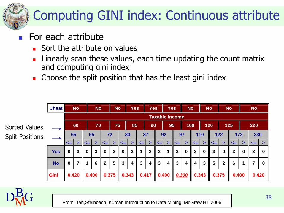
Computing GINI index: Continuous attribute
◼ For each attribute◼ Sort the attribute on values
◼ Linearly scan these values, each time updating the count matrix and computing gini index
◼ Choose the split position that has the least gini index
Cheat No No No Yes Yes Yes No No No No
Taxable Income
60 70 75 85 90 95 100 120 125 220
55 65 72 80 87 92 97 110 122 172 230
<= > <= > <= > <= > <= > <= > <= > <= > <= > <= > <= >
Yes 0 3 0 3 0 3 0 3 1 2 2 1 3 0 3 0 3 0 3 0 3 0
No 0 7 1 6 2 5 3 4 3 4 3 4 3 4 4 3 5 2 6 1 7 0
Gini 0.420 0.400 0.375 0.343 0.417 0.400 0.300 0.343 0.375 0.400 0.420
Split Positions
Sorted Values
From: Tan,Steinbach, Kumar, Introduction to Data Mining, McGraw Hill 2006

39DBMG
Entropy impurity measure (INFO)
◼ Entropy at a given node t
p( j | t) is the relative frequency of class j at node t
◼ Maximum (log nc) when records are equally distributed among all classes, implying higher impurity degree
◼ Minimum (0.0) when all records belong to one class, implying lower impurity degree
◼ Entropy based computations are similar to GINI index computations
From: Tan,Steinbach, Kumar, Introduction to Data Mining, McGraw Hill 2006
−=j
tjptjptEntropy )|(log)|()(2

40DBMG
Examples for computing entropy
C1 0
C2 6
C1 2
C2 4
C1 1
C2 5
P(C1) = 0/6 = 0 P(C2) = 6/6 = 1
Entropy = – 0 log 0 – 1 log 1 = – 0 – 0 = 0
P(C1) = 1/6 P(C2) = 5/6
Entropy = – (1/6) log2 (1/6) – (5/6) log2 (5/6) = 0.65
P(C1) = 2/6 P(C2) = 4/6
Entropy = – (2/6) log2 (2/6) – (4/6) log2 (4/6) = 0.92
−=j
tjptjptEntropy )|(log)|()(2
From: Tan,Steinbach, Kumar, Introduction to Data Mining, McGraw Hill 2006
41DBMG
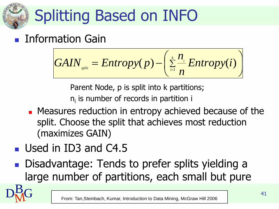
Splitting Based on INFO
◼ Information Gain
Parent Node, p is split into k partitions;
ni is number of records in partition i
◼ Measures reduction in entropy achieved because of the split. Choose the split that achieves most reduction (maximizes GAIN)
◼ Used in ID3 and C4.5
◼ Disadvantage: Tends to prefer splits yielding a large number of partitions, each small but pure
−=
=
k
i
i
splitiEntropy
n
npEntropyGAIN
1
)()(
From: Tan,Steinbach, Kumar, Introduction to Data Mining, McGraw Hill 2006
42DBMG
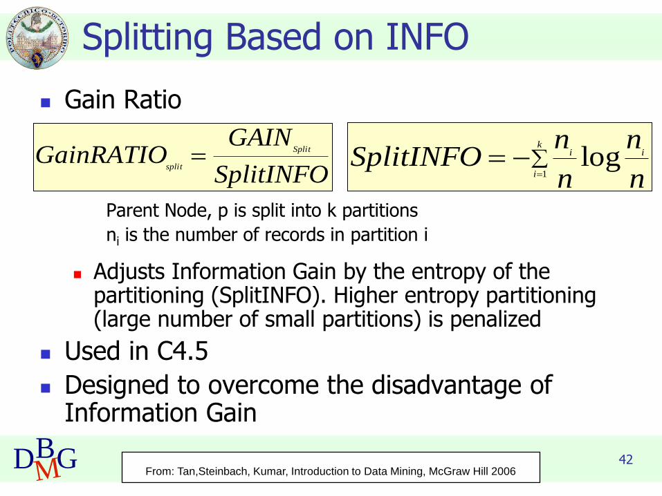
Splitting Based on INFO
◼ Gain Ratio
Parent Node, p is split into k partitions
ni is the number of records in partition i
◼ Adjusts Information Gain by the entropy of the partitioning (SplitINFO). Higher entropy partitioning (large number of small partitions) is penalized
◼ Used in C4.5
◼ Designed to overcome the disadvantage of Information Gain
SplitINFO
GAINGainRATIO Split
split=
=
−=k
i
ii
n
n
n
nSplitINFO
1
log
From: Tan,Steinbach, Kumar, Introduction to Data Mining, McGraw Hill 2006

45DBMG
Comparison among splitting criteria
For a 2-class problem
From: Tan,Steinbach, Kumar, Introduction to Data Mining, McGraw Hill 2006

46DBMG
Stopping Criteria for Tree Induction
◼ Stop expanding a node when all the records belong to the same class
◼ Stop expanding a node when all the records have similar attribute values
◼ Early termination
◼ Pre-pruning
◼ Post-pruning
From: Tan,Steinbach, Kumar, Introduction to Data Mining, McGraw Hill 2006

47DBMG
Underfitting and Overfitting
Overfitting
Underfitting: when model is too simple, both training and test errors are large
From: Tan,Steinbach, Kumar, Introduction to Data Mining, McGraw Hill 2006

48DBMG
Overfitting due to Noise
Decision boundary is distorted by noise point
From: Tan,Steinbach, Kumar, Introduction to Data Mining, McGraw Hill 2006

49DBMG
How to address overfitting
◼ Pre-Pruning (Early Stopping Rule)
◼ Stop the algorithm before it becomes a fully-grown tree
◼ Typical stopping conditions for a node
◼ Stop if all instances belong to the same class
◼ Stop if all the attribute values are the same
◼ More restrictive conditions
◼ Stop if number of instances is less than some user-specified threshold
◼ Stop if class distribution of instances are independent of the available features (e.g., using 2 test)
◼ Stop if expanding the current node does not improve impuritymeasures (e.g., Gini or information gain)
From: Tan,Steinbach, Kumar, Introduction to Data Mining, McGraw Hill 2006

50DBMG
How to address overfitting
◼ Post-pruning
◼ Grow decision tree to its entirety
◼ Trim the nodes of the decision tree in a bottom-up fashion
◼ If generalization error improves after trimming, replace sub-tree by a leaf node.
◼ Class label of leaf node is determined from majority class of instances in the sub-tree
From: Tan,Steinbach, Kumar, Introduction to Data Mining, McGraw Hill 2006

51DBMG
Data fragmentation
◼ Number of instances gets smaller as you traverse down the tree
◼ Number of instances at the leaf nodes could be too small to make any statistically significant decision
From: Tan,Steinbach, Kumar, Introduction to Data Mining, McGraw Hill 2006

52DBMG
Handling missing attribute values
◼ Missing values affect decision tree construction in three different ways
◼ Affect how impurity measures are computed
◼ Affect how to distribute instances with missing value to child nodes
◼ Affect how a test instance with missing value is classified
From: Tan,Steinbach, Kumar, Introduction to Data Mining, McGraw Hill 2006

56DBMG
Decision boundary
y < 0.33?
: 0
: 3
: 4
: 0
y < 0.47?
: 4
: 0
: 0
: 4
x < 0.43?
Yes
Yes
No
No Yes No
0 0.1 0.2 0.3 0.4 0.5 0.6 0.7 0.8 0.9 10
0.1
0.2
0.3
0.4
0.5
0.6
0.7
0.8
0.9
1
x
y
• Border line between two neighboring regions of different classes is known as decision boundary
• Decision boundary is parallel to axes because test condition involves a single attribute at-a-time
From: Tan,Steinbach, Kumar, Introduction to Data Mining, McGraw Hill 2006
57DBMG
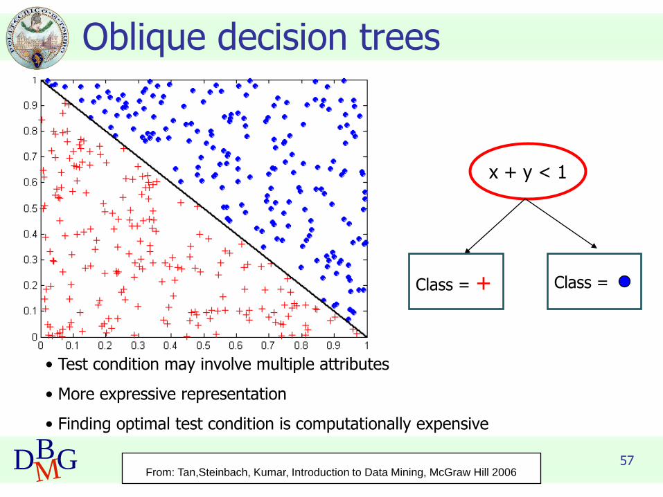
Oblique decision trees
x + y < 1
Class = + Class =
• Test condition may involve multiple attributes
• More expressive representation
• Finding optimal test condition is computationally expensive
From: Tan,Steinbach, Kumar, Introduction to Data Mining, McGraw Hill 2006

59DBMG
◼ Accuracy◼ For simple datasets,
comparable to otherclassification techniques
◼ Interpretability◼ Model is interpretable for
small trees
◼ Single predictions are interpretable
◼ Incrementality◼ Not incremental
Evaluation of decision trees
◼ Efficiency◼ Fast model building
◼ Very fast classification
◼ Scalability◼ Scalable both in training set
size and attribute number
◼ Robustness◼ Difficult management of
missing data

Data Base and Data Mining Group of Politecnico di Torino
DBMG
Random Forest
Elena BaralisPolitecnico di Torino

61DBMG
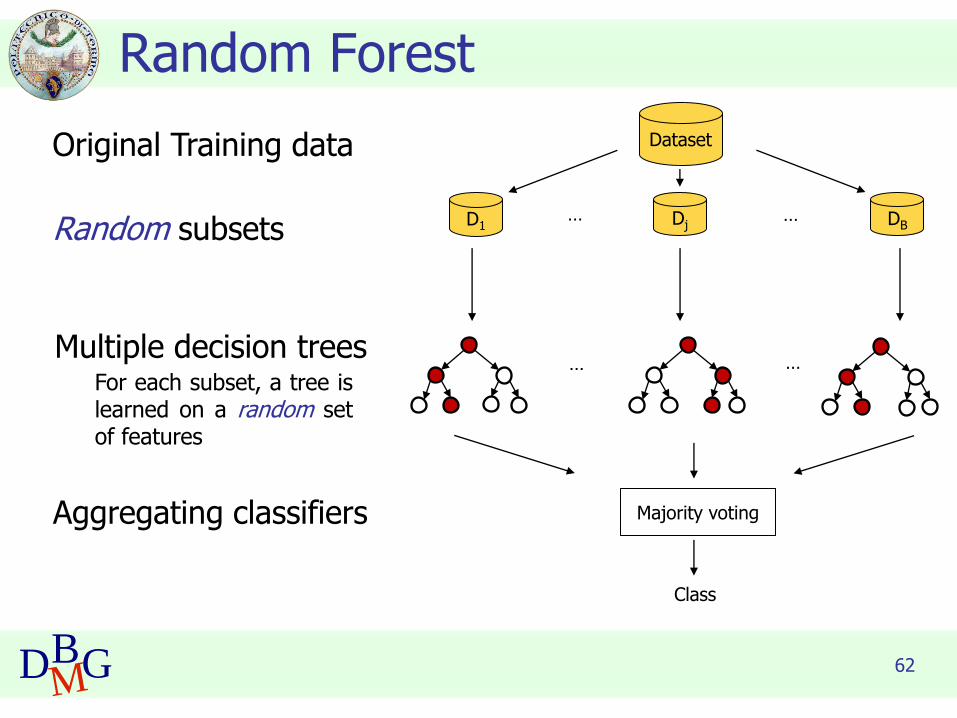
Random Forest
◼ Ensemble learning technique
◼ multiple base models are combined
◼ to improve accuracy and stability
◼ to avoid overfitting
◼ Random forest = set of decision trees◼ a number of decision trees are built at training
time
◼ the class is assigned by majority voting
Bibliography: Hastie, Tibshirani, Friedman, The Elements of Statistical Learning, Springer, 2009
62DBMG
Random Forest
DatasetOriginal Training data
D1 Dj DB… …
Random subsets
Majority voting
Class
Aggregating classifiers
Multiple decision trees… …
For each subset, a tree islearned on a random setof features

63DBMG
Bootstrap aggregation
◼ Given a training set D of n instances, it selects B times a random sample with replacement from D and trains trees on these dataset samples
◼ For b = 1, ..., B
◼ Sample with replacement n’ training examples, n’≤n
◼ A dataset subset Db is generated
◼ Train a classification tree on Db

64DBMG
Feature bagging
◼ Selects, for each candidate split in the learning process, a random subset of the features
◼ Being p the number of features, √𝑝 features are typically selected
◼ Trees are decorrelated
◼ Feature subsets are sampled randomly, hence different features can be selected as best attributes for the split

65DBMG
Random Forest – Algorithm Recap
◼
67DBMG
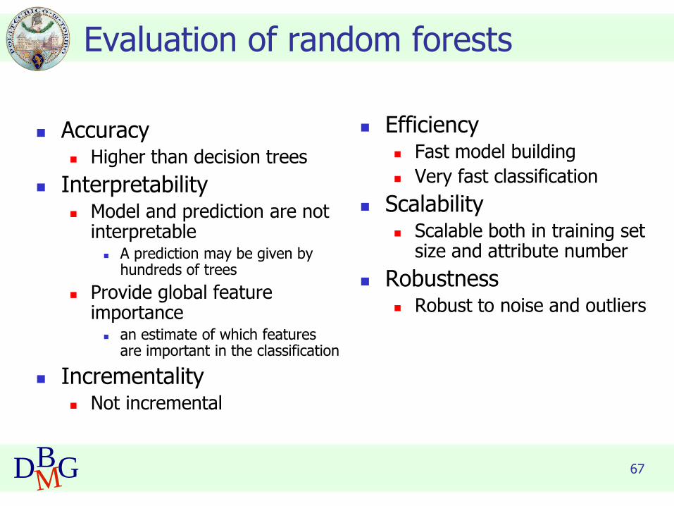
◼ Accuracy◼ Higher than decision trees
◼ Interpretability◼ Model and prediction are not
interpretable◼ A prediction may be given by
hundreds of trees
◼ Provide global feature importance
◼ an estimate of which features are important in the classification
◼ Incrementality◼ Not incremental
Evaluation of random forests
◼ Efficiency◼ Fast model building
◼ Very fast classification
◼ Scalability◼ Scalable both in training set
size and attribute number
◼ Robustness◼ Robust to noise and outliers

Data Base and Data Mining Group of Politecnico di Torino
DBMG
Rule-based classification
Elena BaralisPolitecnico di Torino
69DBMG
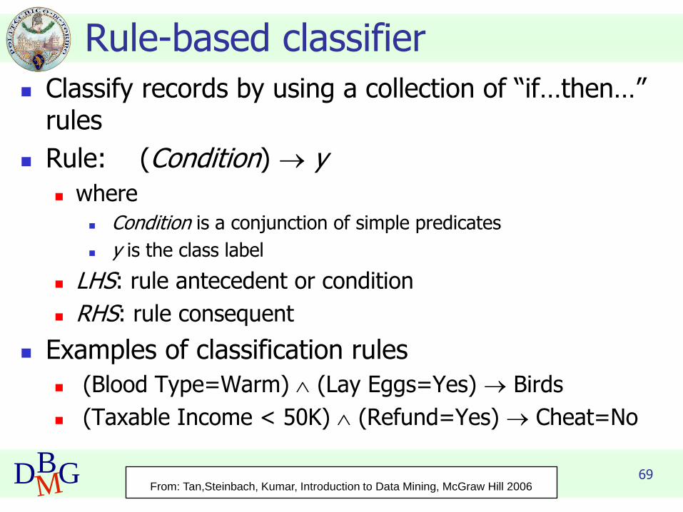
Rule-based classifier
◼ Classify records by using a collection of “if…then…” rules
◼ Rule: (Condition) → y◼ where
◼ Condition is a conjunction of simple predicates
◼ y is the class label
◼ LHS: rule antecedent or condition
◼ RHS: rule consequent
◼ Examples of classification rules
◼ (Blood Type=Warm) (Lay Eggs=Yes) → Birds
◼ (Taxable Income < 50K) (Refund=Yes) → Cheat=No
From: Tan,Steinbach, Kumar, Introduction to Data Mining, McGraw Hill 2006

70DBMG
Rule-based Classifier (Example)
R1: (Give Birth = no) (Can Fly = yes) → Birds
R2: (Give Birth = no) (Live in Water = yes) → Fishes
R3: (Give Birth = yes) (Blood Type = warm) → Mammals
R4: (Give Birth = no) (Can Fly = no) → Reptiles
R5: (Live in Water = sometimes) → Amphibians
Name Blood Type Give Birth Can Fly Live in Water Class
human warm yes no no mammalspython cold no no no reptilessalmon cold no no yes fisheswhale warm yes no yes mammalsfrog cold no no sometimes amphibianskomodo cold no no no reptilesbat warm yes yes no mammalspigeon warm no yes no birdscat warm yes no no mammalsleopard shark cold yes no yes fishesturtle cold no no sometimes reptilespenguin warm no no sometimes birdsporcupine warm yes no no mammalseel cold no no yes fishessalamander cold no no sometimes amphibiansgila monster cold no no no reptilesplatypus warm no no no mammalsowl warm no yes no birdsdolphin warm yes no yes mammalseagle warm no yes no birds
From: Tan,Steinbach, Kumar, Introduction to Data Mining, McGraw Hill 2006
71DBMG
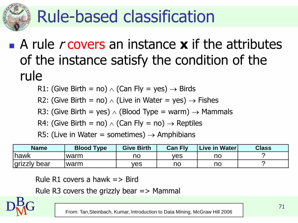
Rule-based classification
◼ A rule r covers an instance x if the attributes of the instance satisfy the condition of the rule
R1: (Give Birth = no) (Can Fly = yes) → Birds
R2: (Give Birth = no) (Live in Water = yes) → Fishes
R3: (Give Birth = yes) (Blood Type = warm) → Mammals
R4: (Give Birth = no) (Can Fly = no) → Reptiles
R5: (Live in Water = sometimes) → Amphibians
Rule R1 covers a hawk => Bird
Rule R3 covers the grizzly bear => Mammal
Name Blood Type Give Birth Can Fly Live in Water Class
hawk warm no yes no ?grizzly bear warm yes no no ?
From: Tan,Steinbach, Kumar, Introduction to Data Mining, McGraw Hill 2006

72DBMG
Rule-based classification
R1: (Give Birth = no) (Can Fly = yes) → Birds
R2: (Give Birth = no) (Live in Water = yes) → Fishes
R3: (Give Birth = yes) (Blood Type = warm) → Mammals
R4: (Give Birth = no) (Can Fly = no) → Reptiles
R5: (Live in Water = sometimes) → Amphibians
A lemur triggers (only) rule R3, so it is classified as a mammal
A turtle triggers both R4 and R5
A dogfish shark triggers none of the rules
Name Blood Type Give Birth Can Fly Live in Water Class
lemur warm yes no no ?turtle cold no no sometimes ?dogfish shark cold yes no yes ?
From: Tan,Steinbach, Kumar, Introduction to Data Mining, McGraw Hill 2006

73DBMG
Characteristics of rules
◼ Mutually exclusive rules
◼ Two rule conditions can’t be true at the same time
◼ Every record is covered by at most one rule
◼ Exhaustive rules
◼ Classifier rules account for every possible combination of attribute values
◼ Each record is covered by at least one rule

74DBMG
From decision trees to rules
YESYESNONO
NONO
NONO
Yes No
{Married}{Single,
Divorced}
< 80K > 80K
Taxable
Income
Marital
Status
RefundClassification Rules
(Refund=Yes) ==> No
(Refund=No, Marital Status={Single,Divorced},
Taxable Income<80K) ==> No
(Refund=No, Marital Status={Single,Divorced},
Taxable Income>80K) ==> Yes
(Refund=No, Marital Status={Married}) ==> No
Rules are mutually exclusive and exhaustive
Rule set contains as much information as the tree
From: Tan,Steinbach, Kumar, Introduction to Data Mining, McGraw Hill 2006

75DBMG
Rules can be simplified
YESYESNONO
NONO
NONO
Yes No
{Married}{Single,
Divorced}
< 80K > 80K
Taxable
Income
Marital
Status
Refund
Tid Refund Marital Status
Taxable Income Cheat
1 Yes Single 125K No
2 No Married 100K No
3 No Single 70K No
4 Yes Married 120K No
5 No Divorced 95K Yes
6 No Married 60K No
7 Yes Divorced 220K No
8 No Single 85K Yes
9 No Married 75K No
10 No Single 90K Yes 10
Initial Rule: (Refund=No) (Status=Married) → No
Simplified Rule: (Status=Married) → No
From: Tan,Steinbach, Kumar, Introduction to Data Mining, McGraw Hill 2006

76DBMG
Effect of rule simplification
◼ Rules are no longer mutually exclusive
◼ A record may trigger more than one rule
◼ Solution?
◼ Ordered rule set
◼ Unordered rule set – use voting schemes
◼ Rules are no longer exhaustive
◼ A record may not trigger any rules
◼ Solution?
◼ Use a default class
From: Tan,Steinbach, Kumar, Introduction to Data Mining, McGraw Hill 2006
77DBMG
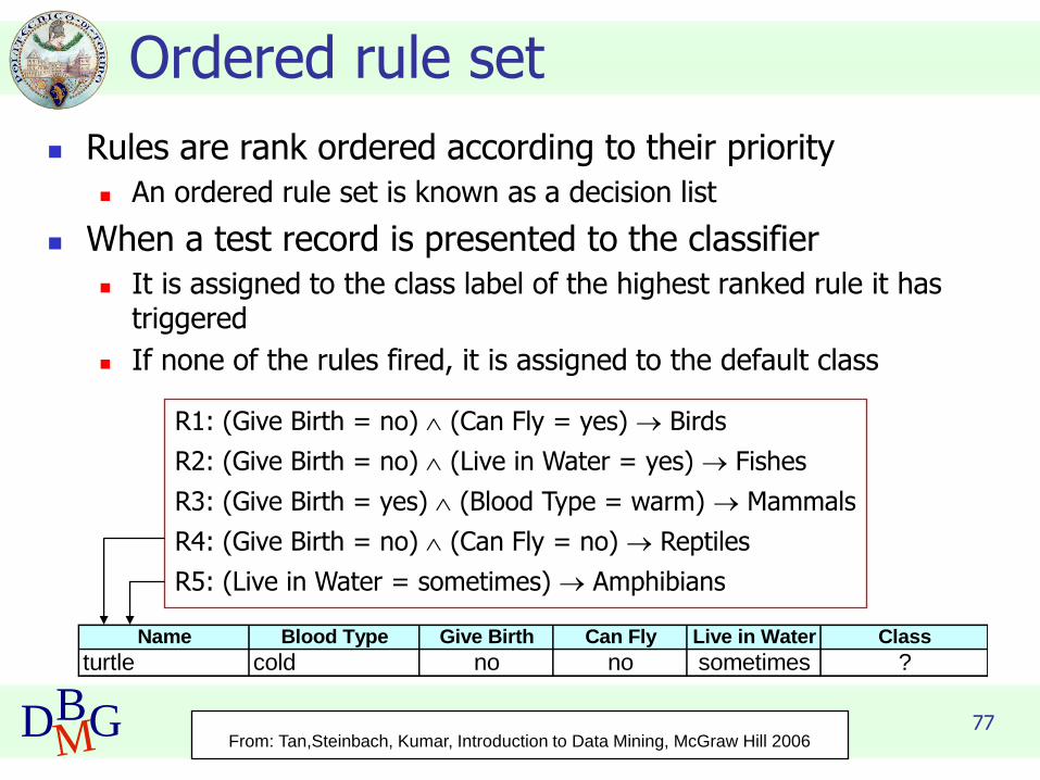
Ordered rule set
◼ Rules are rank ordered according to their priority
◼ An ordered rule set is known as a decision list
◼ When a test record is presented to the classifier
◼ It is assigned to the class label of the highest ranked rule it has triggered
◼ If none of the rules fired, it is assigned to the default class
R1: (Give Birth = no) (Can Fly = yes) → Birds
R2: (Give Birth = no) (Live in Water = yes) → Fishes
R3: (Give Birth = yes) (Blood Type = warm) → Mammals
R4: (Give Birth = no) (Can Fly = no) → Reptiles
R5: (Live in Water = sometimes) → Amphibians
Name Blood Type Give Birth Can Fly Live in Water Class
turtle cold no no sometimes ?
From: Tan,Steinbach, Kumar, Introduction to Data Mining, McGraw Hill 2006

78DBMG
Building classification rules
◼ Direct Method◼ Extract rules directly from data
◼ e.g.: RIPPER, CN2, Holte’s 1R
◼ Indirect Method◼ Extract rules from other classification models (e.g.
decision trees, neural networks, etc).
◼ e.g: C4.5rules
From: Tan,Steinbach, Kumar, Introduction to Data Mining, McGraw Hill 2006

80DBMG
◼ Accuracy◼ Higher than decision trees
◼ Interpretability◼ Model and prediction are
interpretable
◼ Incrementality◼ Not incremental
Evaluation of rule based classifiers
◼ Efficiency◼ Fast model building
◼ Very fast classification
◼ Scalability◼ Scalable both in training set
size and attribute number
◼ Robustness◼ Robust to outliers
Data Base and Data Mining Group of Politecnico di Torino
DBMG
Associative classification
Elena BaralisPolitecnico di Torino

82DBMG
Associative classification
◼ The classification model is defined by means of association rules
(Condition) → y
◼ rule body is an itemset
◼ Model generation
◼ Rule selection & sorting
◼ based on support, confidence and correlation thresholds
◼ Rule pruning
◼ Database coverage: the training set is covered by selecting topmost rules according to previous sort

83DBMG
◼ Accuracy◼ Higher than decision trees
and rule-based classifiers◼ correlation among attributes is
considered
◼ Interpretability◼ Model and prediction are
interpretable
◼ Incrementality◼ Not incremental
Evaluation of associative classifiers
◼ Efficiency◼ Rule generation may be slow
◼ It depends on support threshold
◼ Very fast classification
◼ Scalability◼ Scalable in training set size
◼ Reduced scalability in attribute number
◼ Rule generation may become unfeasible
◼ Robustness◼ Unaffected by missing data
◼ Robust to outliers

Data Base and Data Mining Group of Politecnico di Torino
DBMG
K-Nearest Neighbor
Elena BaralisPolitecnico di Torino

86DBMG
Instance-Based Classifiers
Atr1 ……... AtrN Class
A
B
B
C
A
C
B
Set of Stored Cases
Atr1 ……... AtrN
Unseen Case
• Store the training records
• Use training records to predict the class label of unseen cases
From: Tan,Steinbach, Kumar, Introduction to Data Mining, McGraw Hill 2006

87DBMG
Instance Based Classifiers
◼ Examples
◼ Rote-learner
◼ Memorizes entire training data and performs classification only if attributes of record match one of the training examples exactly
◼ Nearest neighbor
◼ Uses k “closest” points (nearest neighbors) for performing classification
From: Tan,Steinbach, Kumar, Introduction to Data Mining, McGraw Hill 2006

88DBMG
Nearest-Neighbor Classifiers
Requires
– The set of stored records
– Distance Metric to compute distance between records
– The value of k, the number of nearest neighbors to retrieve
To classify an unknown record
– Compute distance to other training records
– Identify k nearest neighbors
– Use class labels of nearest neighbors to determine the class label of unknown record (e.g., by taking majority vote)
Unknown record
From: Tan,Steinbach, Kumar, Introduction to Data Mining, McGraw Hill 2006

89DBMG
Definition of Nearest Neighbor
X X X
(a) 1-nearest neighbor (b) 2-nearest neighbor (c) 3-nearest neighbor
K-nearest neighbors of a record x are data points that have the k smallest distance to x
From: Tan,Steinbach, Kumar, Introduction to Data Mining, McGraw Hill 2006

90DBMG
1 nearest-neighbor
Voronoi Diagram
From: Tan,Steinbach, Kumar, Introduction to Data Mining, McGraw Hill 2006
91DBMG
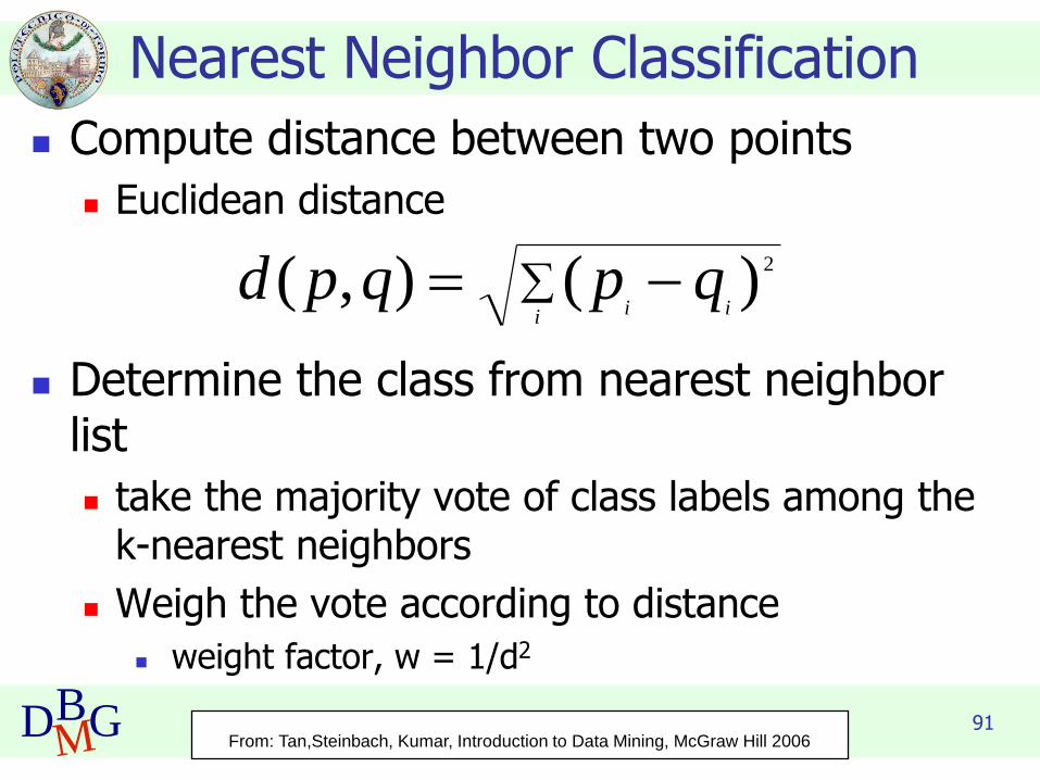
Nearest Neighbor Classification
◼ Compute distance between two points
◼ Euclidean distance
◼ Determine the class from nearest neighbor list
◼ take the majority vote of class labels among the k-nearest neighbors
◼ Weigh the vote according to distance
◼ weight factor, w = 1/d2
−=i ii
qpqpd 2)(),(
From: Tan,Steinbach, Kumar, Introduction to Data Mining, McGraw Hill 2006

92DBMG
Nearest Neighbor Classification
◼ Choosing the value of k:◼ If k is too small, sensitive to noise points
◼ If k is too large, neighborhood may include points from other classes
X
From: Tan,Steinbach, Kumar, Introduction to Data Mining, McGraw Hill 2006
93DBMG
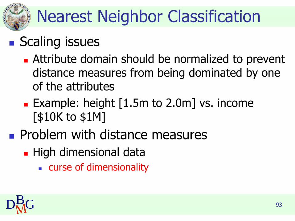
Nearest Neighbor Classification
◼ Scaling issues
◼ Attribute domain should be normalized to prevent distance measures from being dominated by one of the attributes
◼ Example: height [1.5m to 2.0m] vs. income [$10K to $1M]
◼ Problem with distance measures
◼ High dimensional data
◼ curse of dimensionality
94DBMG
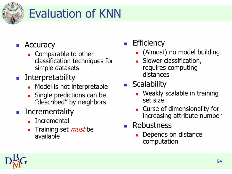
◼ Accuracy◼ Comparable to other
classification techniques for simple datasets
◼ Interpretability◼ Model is not interpretable
◼ Single predictions can be ˮdescribedˮ by neighbors
◼ Incrementality◼ Incremental
◼ Training set must be available
Evaluation of KNN
◼ Efficiency◼ (Almost) no model building
◼ Slower classification, requires computing distances
◼ Scalability◼ Weakly scalable in training
set size
◼ Curse of dimensionality for increasing attribute number
◼ Robustness◼ Depends on distance
computation

Data Base and Data Mining Group of Politecnico di Torino
DBMG
Bayesian Classification
Elena BaralisPolitecnico di Torino

96DBMG
Bayes theorem
◼ Let C and X be random variables
P(C,X) = P(C|X) P(X)
P(C,X) = P(X|C) P(C)
◼ Hence
P(C|X) P(X) = P(X|C) P(C)
◼ and also
P(C|X) = P(X|C) P(C) / P(X)

97DBMG
Bayesian classification
◼ Let the class attribute and all data attributes be random variables◼ C = any class label
◼ X = <x1,…,xk> record to be classified
◼ Bayesian classification◼ compute P(C|X) for all classes
◼ probability that record X belongs to C
◼ assign X to the class with maximal P(C|X)
◼ Applying Bayes theorem
P(C|X) = P(X|C)·P(C) / P(X)◼ P(X) constant for all C, disregarded for maximum computation
◼ P(C) a priori probability of C
P(C) = Nc/N
98DBMG
Bayesian classification
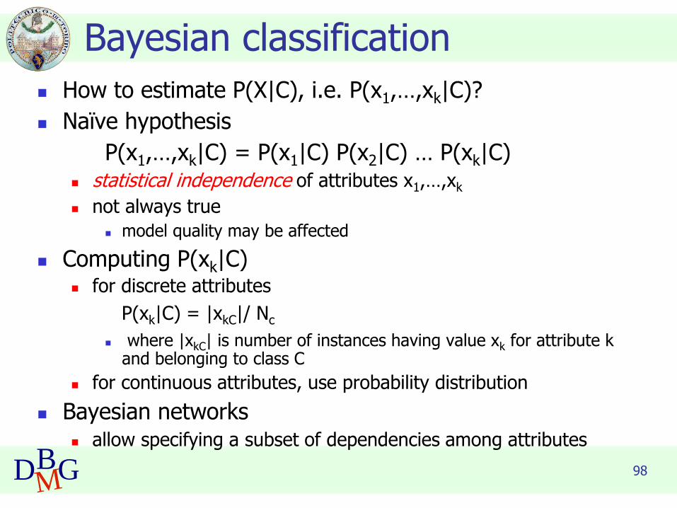
◼ How to estimate P(X|C), i.e. P(x1,…,xk|C)?
◼ Naïve hypothesis
P(x1,…,xk|C) = P(x1|C) P(x2|C) … P(xk|C)◼ statistical independence of attributes x1,…,xk
◼ not always true
◼ model quality may be affected
◼ Computing P(xk|C)◼ for discrete attributes
P(xk|C) = |xkC|/ Nc
◼ where |xkC| is number of instances having value xk for attribute k and belonging to class C
◼ for continuous attributes, use probability distribution
◼ Bayesian networks◼ allow specifying a subset of dependencies among attributes

99DBMG
Bayesian classification: ExampleOutlook Temperature Humidity Windy Class
sunny hot high false N
sunny hot high true N
overcast hot high false P
rain mild high false P
rain cool normal false P
rain cool normal true N
overcast cool normal true P
sunny mild high false N
sunny cool normal false P
rain mild normal false P
sunny mild normal true P
overcast mild high true P
overcast hot normal false P
rain mild high true N
From: Han, Kamber,”Data mining; Concepts and Techniques”, Morgan Kaufmann 2006

100DBMG
Bayesian classification: Exampleoutlook
P(sunny|p) = 2/9 P(sunny|n) = 3/5
P(overcast|p) = 4/9 P(overcast|n) = 0
P(rain|p) = 3/9 P(rain|n) = 2/5
temperature
P(hot|p) = 2/9 P(hot|n) = 2/5
P(mild|p) = 4/9 P(mild|n) = 2/5
P(cool|p) = 3/9 P(cool|n) = 1/5
humidity
P(high|p) = 3/9 P(high|n) = 4/5
P(normal|p) = 6/9 P(normal|n) = 2/5
windy
P(true|p) = 3/9 P(true|n) = 3/5
P(false|p) = 6/9 P(false|n) = 2/5
P(p) = 9/14
P(n) = 5/14
From: Han, Kamber,”Data mining; Concepts and Techniques”, Morgan Kaufmann 2006

101DBMG
Bayesian classification: Example
◼ Data to be labeled
X = <rain, hot, high, false>
◼ For class p
P(X|p)·P(p) = = P(rain|p)·P(hot|p)·P(high|p)·P(false|p)·P(p) = 3/9·2/9·3/9·6/9·9/14 = 0.010582
◼ For class n
P(X|n)·P(n) = = P(rain|n)·P(hot|n)·P(high|n)·P(false|n)·P(n) = 2/5·2/5·4/5·2/5·5/14 = 0.018286
From: Han, Kamber,”Data mining; Concepts and Techniques”, Morgan Kaufmann 2006

102DBMG
◼ Accuracy◼ Similar or lower than decision
trees◼ Naïve hypothesis simplifies
model
◼ Interpretability◼ Model and prediction are not
interpretable◼ The weights of contributions in a
single prediction may be used to explain
◼ Incrementality◼ Fully incremental
◼ Does not require availability of training data
Evaluation of Naïve Bayes Classifiers
◼ Efficiency◼ Fast model building
◼ Very fast classification
◼ Scalability◼ Scalable both in training set
size and attribute number
◼ Robustness◼ Affected by attribute
correlation

Data Base and Data Mining Group of Politecnico di Torino
DBMG
Support Vector Machines
Elena BaralisPolitecnico di Torino
104DBMG
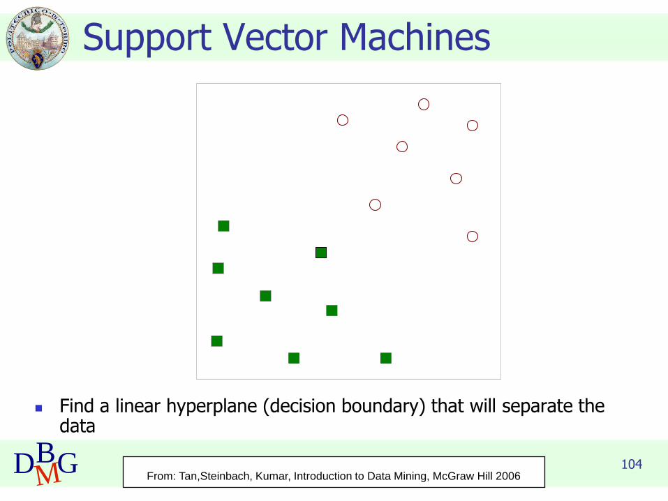
Support Vector Machines
◼ Find a linear hyperplane (decision boundary) that will separate the data
From: Tan,Steinbach, Kumar, Introduction to Data Mining, McGraw Hill 2006
105DBMG
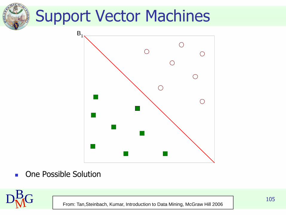
Support Vector Machines
◼ One Possible Solution
B1
From: Tan,Steinbach, Kumar, Introduction to Data Mining, McGraw Hill 2006
106DBMG
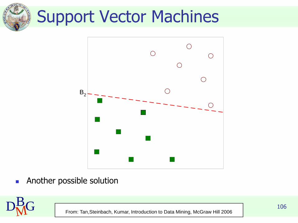
Support Vector Machines
◼ Another possible solution
B2
From: Tan,Steinbach, Kumar, Introduction to Data Mining, McGraw Hill 2006

107DBMG
Support Vector Machines
◼ Other possible solutions
B2
From: Tan,Steinbach, Kumar, Introduction to Data Mining, McGraw Hill 2006

108DBMG
Support Vector Machines
◼ Which one is better? B1 or B2?
◼ How do you define better?
B1
B2
From: Tan,Steinbach, Kumar, Introduction to Data Mining, McGraw Hill 2006

109DBMG
Support Vector Machines
◼ Find hyperplane maximizes the margin => B1 is better than B2
B1
B2
b11
b12
b21
b22
margin
From: Tan,Steinbach, Kumar, Introduction to Data Mining, McGraw Hill 2006

110DBMG
Nonlinear Support Vector Machines
◼ What if decision boundary is not linear?
From: Tan,Steinbach, Kumar, Introduction to Data Mining, McGraw Hill 2006

111DBMG
Nonlinear Support Vector Machines
◼ Transform data into higher dimensional space
From: Tan,Steinbach, Kumar, Introduction to Data Mining, McGraw Hill 2006

112DBMG
◼ Accuracy◼ Among best performers
◼ Interpretability◼ Model and prediction are not
interpretable◼ Black box model
◼ Incrementality◼ Not incremental
Evaluation of Support Vector Machines
◼ Efficiency◼ Model building requires
significant parameter tuning
◼ Very fast classification
◼ Scalability◼ Medium scalable both in
training set size and attribute number
◼ Robustness◼ Robust to noise and outliers

Data Base and Data Mining Group of Politecnico di Torino
DBMG
Artificial Neural Networks
Elena BaralisPolitecnico di Torino

114DBMG
Artificial Neural Networks
◼ Inspired to the structure of the human brain◼ Neurons as elaboration units
◼ Synapses as connection network

115DBMG
Artificial Neural Networks
◼ Different tasks, different architectures
numerical vectors classification: feed forward NN (FFNN)
image understanding: convolutional NN (CNN) time series analysis: recurrent NN (RNN)
denoising: auto-encoders
116DBMG
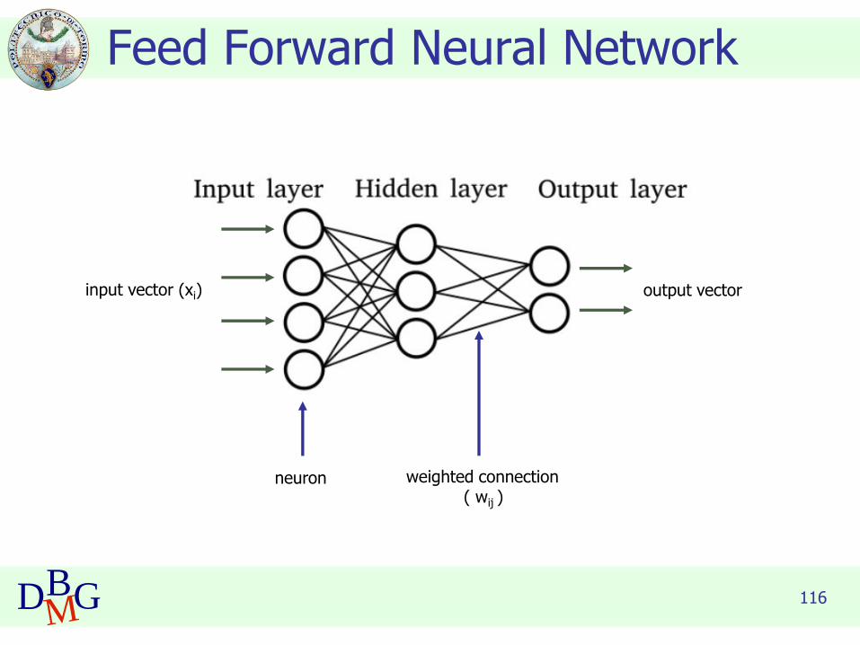
Feed Forward Neural Network
neuron weighted connection( wij )
input vector (xi) output vector

118DBMG
Structure of a neuron
mk-
f
Weighted
sum
Input
vector x
output y
Activation
function
Weight
vector w
w0
w1
wn
x0
x1
xn
From: Han, Kamber,”Data mining; Concepts and Techniques”, Morgan Kaufmann 2006

119DBMG
◼ Activation◼ simulates biological activation to input stymula
◼ provides non-linearity to the computation
◼ may help to saturate neuron outputs in fixed ranges
Activation Functions

120DBMG
◼ Sigmoid, tanh
◼ saturate input value in a fixed range
◼ non linear for all the input scale
◼ typically used by FFNNs for both hidden and output layers◼ E.g. sigmoid in output layers allows generating values between 0 and 1
(useful when output must be interpreted as likelihood)
Activation Functions
121DBMG
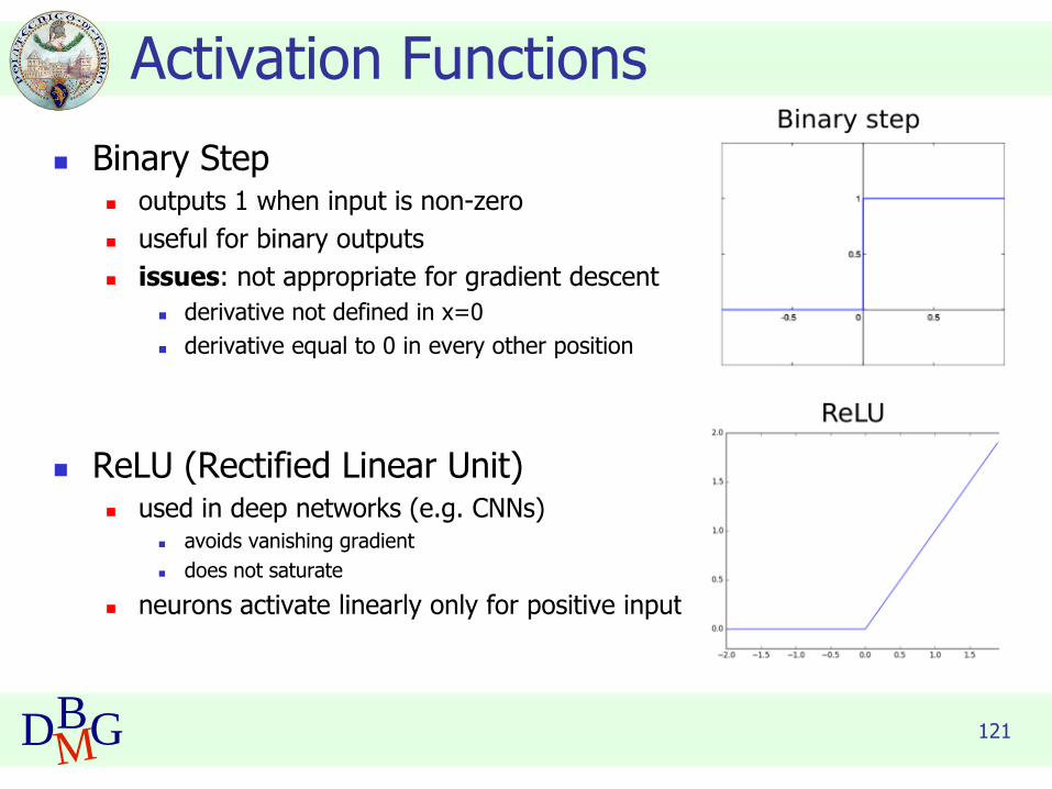
◼ Binary Step◼ outputs 1 when input is non-zero
◼ useful for binary outputs
◼ issues: not appropriate for gradient descent
◼ derivative not defined in x=0
◼ derivative equal to 0 in every other position
◼ ReLU (Rectified Linear Unit)◼ used in deep networks (e.g. CNNs)
◼ avoids vanishing gradient
◼ does not saturate
◼ neurons activate linearly only for positive input
Activation Functions

122DBMG
◼ Softmax◼ differently to other activation functions
◼ it is applied only to the output layer
◼ works by considering all the neurons in the layer
◼ after softmax, the output vector can be interpreted as a discrete distribution of probabilities
◼ e.g. the probabilities for the input pattern of belonging to each class
Activation Functions
output layer
123DBMG
Building a FFNN
◼ For each node, definition of◼ set of weights
◼ offset value
providing the highest accuracy on the training data
◼ Iterative approach on training data instances
124DBMG
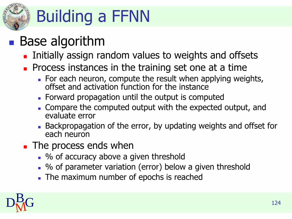
Building a FFNN
◼ Base algorithm◼ Initially assign random values to weights and offsets
◼ Process instances in the training set one at a time◼ For each neuron, compute the result when applying weights,
offset and activation function for the instance
◼ Forward propagation until the output is computed
◼ Compare the computed output with the expected output, and evaluate error
◼ Backpropagation of the error, by updating weights and offset for each neuron
◼ The process ends when◼ % of accuracy above a given threshold
◼ % of parameter variation (error) below a given threshold
◼ The maximum number of epochs is reached

126DBMG
◼ Accuracy◼ Among best performers
◼ Interpretability◼ Model and prediction are not
interpretable◼ Black box model
◼ Incrementality◼ Not incremental
Evaluation of Feed Forward NN
◼ Efficiency◼ Model building requires very
complex parameter tuning◼ It requires significant time
◼ Very fast classification
◼ Scalability◼ Medium scalable both in
training set size and attribute number
◼ Robustness◼ Robust to noise and outliers
◼ Requires large training set◼ Otherwise unstable when
tuning parameters

127DBMG
Convolutional Neural Networks
Convolutional Neural Network (CNN) Architecture
input image predicted class with confidence
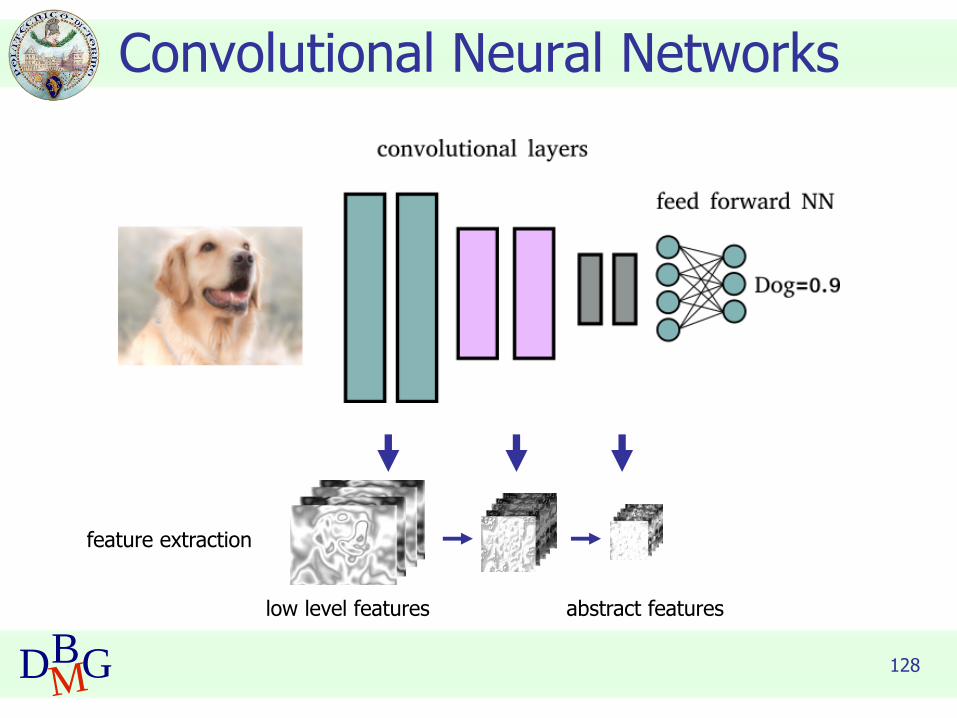
◼ Allow automatically extracting features from images and performing classification
128DBMG
Convolutional Neural Networks
feature extraction
abstract featureslow level features

129DBMG
Convolutional Neural Networks
feature extraction
classification,with softmax activation
abstract featureslow level features

130DBMG
◼ Typical convolutional layer◼ convolution stage: feature extraction by means of (hundreds to
thousands) sliding filters
◼ sliding filters activation: apply activation functions to input tensor
◼ pooling: tensor downsampling
Convolutional Neural Networks
convolution
activation
pooling

131DBMG
◼ Tensors◼ data flowing through CNN layers is represented in the form of tensors
◼ Tensor = N-dimensional vector
◼ Rank = number of dimensions◼ scalar: rank 0
◼ 1-D vector: rank 1
◼ 2-D matrix: rank 2
◼ Shape = number of elements for each dimension◼ e.g. a vector of length 5 has shape [5]
◼ e.g. a matrix w x h, w=5, h=3 has shape [h, w] = [3, 5]
Convolutional Neural Networks
rank-3 tensor with shape[d,h,w] = [4,2,3]

132DBMG
◼ Images◼ rank-3 tensors with shape [d,h,w]
◼ where h=height, w=width, d=image depth (1 for grayscale, 3 for RGB colors)
Convolutional Neural Networks
133DBMG
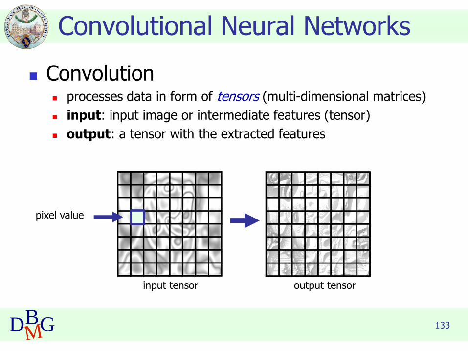
◼ Convolution◼ processes data in form of tensors (multi-dimensional matrices)
◼ input: input image or intermediate features (tensor)
◼ output: a tensor with the extracted features
Convolutional Neural Networks
input tensor output tensor
pixel value

134DBMG
◼ Convolution◼ a sliding filter produces the values of the output tensor
◼ sliding filters contain the trainable weights of the neural network
◼ each convolutional layer contains many (hundreds) filters
Convolutional Neural Networks
input tensoroutput tensor
sliding filter
padding
135DBMG
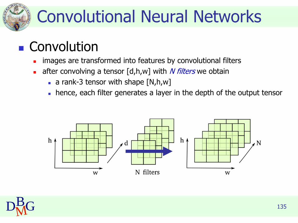
◼ Convolution◼ images are transformed into features by convolutional filters
◼ after convolving a tensor [d,h,w] with N filters we obtain
◼ a rank-3 tensor with shape [N,h,w]
◼ hence, each filter generates a layer in the depth of the output tensor
Convolutional Neural Networks

136DBMG
◼ Activation◼ symulates biological activation to input stymula
◼ provides non-linearity to the computation
◼ ReLU is typically used for CNNs◼ faster training (no vanishing gradients)
◼ does not saturate
◼ faster computation of derivatives for backpropagation
Convolutional Neural Networks
0
0
ReLU

137DBMG
◼ Pooling◼ performs tensor downsampling
◼ sliding filter which replaces tensor values with a summary statistic of the nearby outputs
◼ maxpool is the most common: computes the maximum value as statistic
Convolutional Neural Networks
output tensor
sliding filter

138DBMG
◼ Convolutional layers training◼ during training each sliding filter learns to recognize a particular
pattern in the input tensor
◼ filters in shallow layers recognize textures and edges
◼ filters in deeper layers can recognize objects and parts (e.g. eye, ear or even faces)
Convolutional Neural Networks
shallow filters
deeper filters

139DBMG
◼ Semantic segmentation CNNs◼ allow assigning a class to each pixel of the input image
◼ composed of 2 parts◼ encoder network: convolutional layers to extract abstract features
◼ decoder network: deconvolutional layers to obtain the output image from the extracted features
Convolutional Neural Networks
SegNet neural network
140DBMG
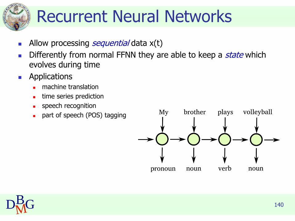
◼ Allow processing sequential data x(t)
◼ Differently from normal FFNN they are able to keep a state which evolves during time
◼ Applications◼ machine translation
◼ time series prediction
◼ speech recognition
◼ part of speech (POS) tagging
Recurrent Neural Networks

141DBMG
Recurrent Neural Networks
instance of the RNN at time t1
◼ RNN execution during time
142DBMG
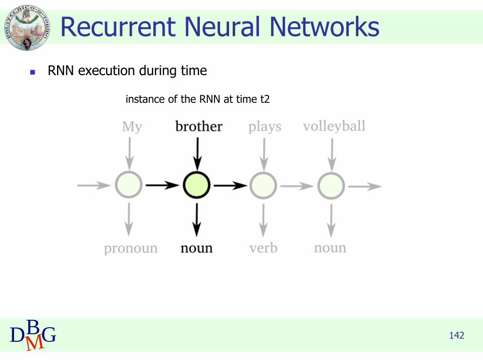
Recurrent Neural Networks
instance of the RNN at time t2
◼ RNN execution during time

143DBMG
Recurrent Neural Networks
instance of the RNN at time t3
◼ RNN execution during time

144DBMG
Recurrent Neural Networks
instance of the RNN at time t4
◼ RNN execution during time

145DBMG
◼ A RNN receives as input a vector x(t) and the state at previous time step s(t-1)
◼ A RNN typically contains many neurons organized in different layers
Recurrent Neural Networks
inputx(t)
outputy(t)
state retroactionw’
w
s(t-1)
internal structure
146DBMG
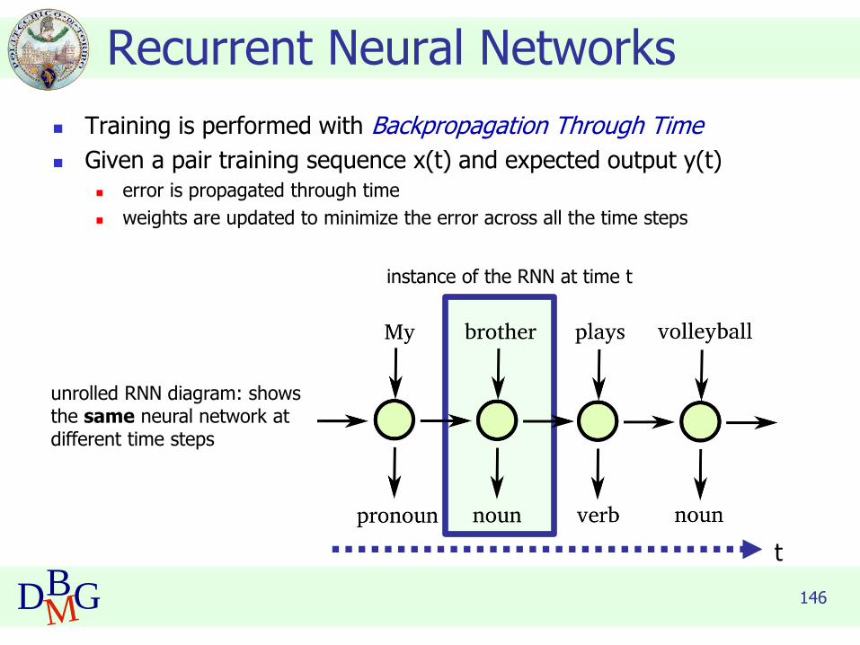
◼ Training is performed with Backpropagation Through Time
◼ Given a pair training sequence x(t) and expected output y(t)◼ error is propagated through time
◼ weights are updated to minimize the error across all the time steps
Recurrent Neural Networks
instance of the RNN at time t
unrolled RNN diagram: shows the same neural network at different time steps
t

147DBMG
◼ Issues
◼ vanishing gradient: error gradient decreases rapidly over time, weights are not properly updated
◼ this makes harder having RNN with long-term memories
◼ Solution: LSTM (Long Short Term Memories)
◼ RNN with “gates” which encourage the state information to flow through long time intervals
Recurrent Neural Networks
LSTM stage
148DBMG
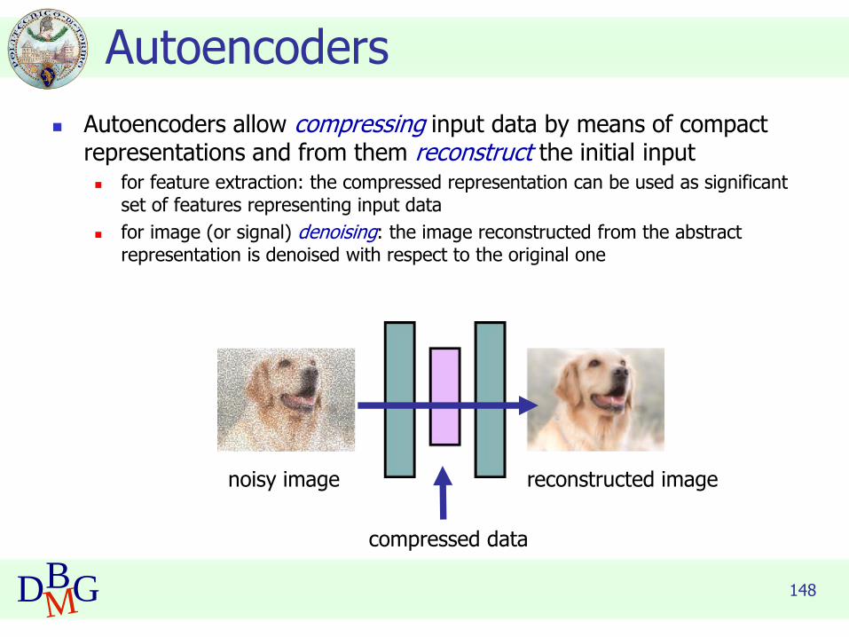
◼ Autoencoders allow compressing input data by means of compact representations and from them reconstruct the initial input◼ for feature extraction: the compressed representation can be used as significant
set of features representing input data
◼ for image (or signal) denoising: the image reconstructed from the abstract representation is denoised with respect to the original one
Autoencoders
reconstructed imagenoisy image
compressed data

149DBMG
◼ Word embeddings associate words to n-dimensional vectors◼ trained on big text collections to model the word distributions in different
sentences and contexts
◼ able to capture the semantic information of each word
◼ words with similar meaning share vectors with similar characteristics
Word Embeddings (Word2Vec)
input word
embedding vector
e(man)=[e1,e2,e3]
e(king)=[e1’,e2’,e3’]man
e1
e2
e3

150DBMG
◼ Since each word is represented with a vector, operations among words (e.g. difference, addition) are allowed
Word Embeddings (Word2Vec)

151DBMG
◼ Semantic relationiships among words are captured by vector positions
Word Embeddings (Word2Vec)
king - man = queen - womanking - man + woman = queen

Data Base and Data Mining Group of Politecnico di Torino
DBMG
Model evaluation
Elena BaralisPolitecnico di Torino

153DBMG
Model evaluation
◼ Methods for performance evaluation
◼ Partitioning techniques for training and test sets
◼ Metrics for performance evaluation
◼ Accuracy, other measures
◼ Techniques for model comparison
◼ ROC curve
154DBMG
Methods for performance evaluation
◼ Objective
◼ reliable estimate of performance
◼ Performance of a model may depend on other factors besides the learning algorithm
◼ Class distribution
◼ Cost of misclassification
◼ Size of training and test sets
From: Tan,Steinbach, Kumar, Introduction to Data Mining, McGraw Hill 2006
155DBMG
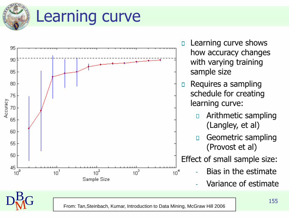
Learning curve
Learning curve shows how accuracy changes with varying training sample size
Requires a sampling schedule for creating learning curve:
Arithmetic sampling(Langley, et al)
Geometric sampling(Provost et al)
Effect of small sample size:
- Bias in the estimate
- Variance of estimate
From: Tan,Steinbach, Kumar, Introduction to Data Mining, McGraw Hill 2006

156DBMG
Partitioning data
◼ Several partitioning techniques◼ holdout
◼ cross validation
◼ Stratified sampling to generate partitions◼ without replacement
◼ Bootstrap◼ Sampling with replacement
157DBMG
Methods of estimation
◼ Partitioning labeled data for training, validation and test
◼ Several partitioning techniques◼ holdout
◼ cross validation
◼ Stratified sampling to generate partitions◼ without replacement
◼ Bootstrap◼ Sampling with replacement

158DBMG
Holdout
◼ Fixed partitioning◼ Typically, may reserve 80% for training, 20%
for test
◼ Other proportions may be appropriate, depending on the dataset size
◼ Appropriate for large datasets◼ may be repeated several times
◼ repeated holdout

159DBMG
Cross validation
◼ Cross validation◼ partition data into k disjoint subsets (i.e., folds)
◼ k-fold: train on k-1 partitions, test on the remaining one◼ repeat for all folds
◼ reliable accuracy estimation, not appropriate for very large datasets
◼ Leave-one-out◼ cross validation for k=n
◼ only appropriate for very small datasets

160DBMG
Model performance estimation
◼ Model training step◼ Building a new model
◼ Model validation step◼ Hyperparameter tuning
◼ Algorithm selection
◼ Model test step◼ Estimation of model performance
161DBMG
Model performance estimation
◼ Typical dataset size◼ Training set 60% of labeled data
◼ Validation set 20% of labeled data
◼ Test set 20% of labeled data
◼ Splitting labeled data◼ Use hold-out to split in
◼ training+validation
◼ test
◼ Use cross validation to split in◼ training
◼ validation

162DBMG
◼ Evaluate the predictive accuracy of a model
◼ Confusion matrix
◼ binary classifier
PREDICTED CLASS
ACTUAL
CLASS
Class=Yes Class=No
Class=Yes a b
Class=No c d
a: TP (true positive)
b: FN (false negative)
c: FP (false positive)
d: TN (true negative)
From: Tan,Steinbach, Kumar, Introduction to Data Mining, McGraw Hill 2006
Metrics for model evaluation
163DBMG
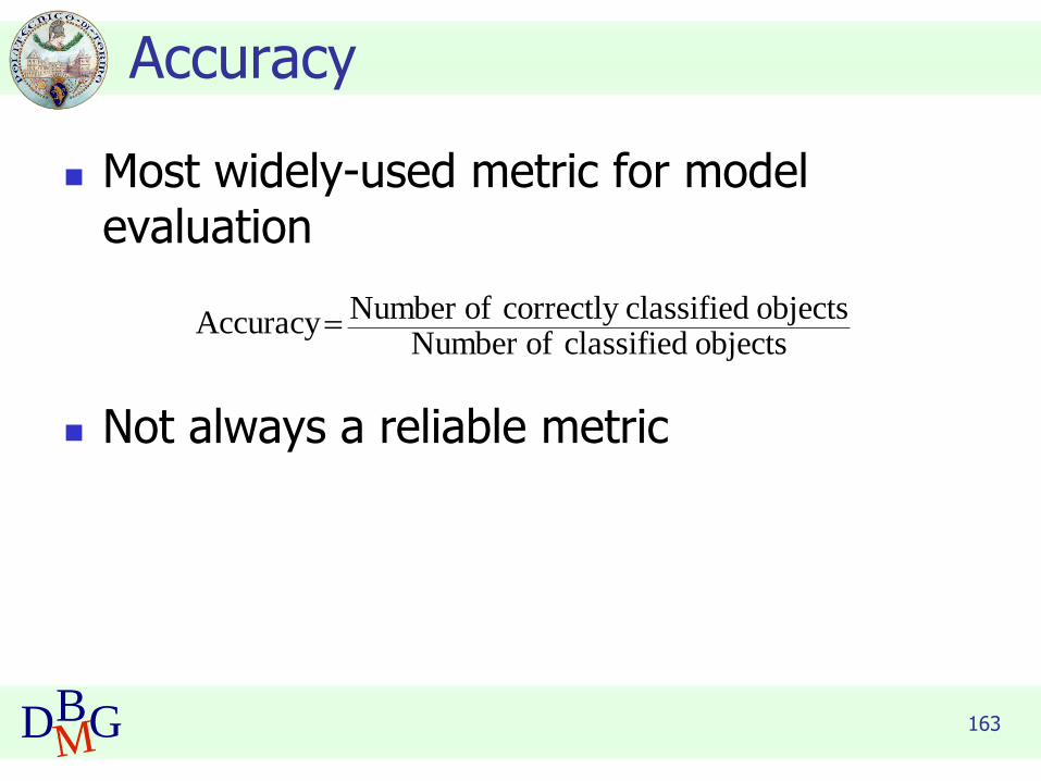
Accuracy
◼ Most widely-used metric for model evaluation
◼ Not always a reliable metric
objects classified ofNumber objects classifiedcorrectly ofNumber Accuracy=

164DBMG
Accuracy
◼ For a binary classifier
PREDICTED CLASS
ACTUAL
CLASS
Class=Yes Class=No
Class=Yes a
(TP)
b
(FN)
Class=No c
(FP)
d
(TN)
FNFPTNTP
TNTP
dcba
da
+++
+=
+++
+=Accuracy
From: Tan,Steinbach, Kumar, Introduction to Data Mining, McGraw Hill 2006

165DBMG
Limitations of accuracy
◼ Consider a binary problem◼ Cardinality of Class 0 = 9900
◼ Cardinality of Class 1 = 100
◼ Model
() → class 0
◼ Model predicts everything to be class 0
◼ accuracy is 9900/10000 = 99.0 %
◼ Accuracy is misleading because the model does not detect any class 1 object
166DBMG
Limitations of accuracy
◼ Classes may have different importance
◼ Misclassification of objects of a given class is more important
◼ e.g., ill patients erroneously assigned to the healthy patients class
◼ Accuracy is not appropriate for◼ unbalanced class label distribution
◼ different class relevance

167DBMG
◼ Evaluate separately for each class C
◼ Maximize
Class specific measures
pr
rp
+=
2(F) measure-F
C tobelonging objects ofNumber C toassignedcorrectly objects ofNumber (r) Recall =
C toassigned objects ofNumber C toassignedcorrectly objects ofNumber (p)Precision =

168DBMG
Class specific measures
cba
a
pr
rp
ba
a
ca
a
++=
+=
+=
+=
2
22(F) measure-F
(r) Recall
(p)Precision
From: Tan,Steinbach, Kumar, Introduction to Data Mining, McGraw Hill 2006
◼ For a binary classification problem
◼ on the confusion matrix, for the positive class

169DBMG
ROC (Receiver Operating Characteristic)
◼ Developed in 1950s for signal detection theory to analyze noisy signals ◼ characterizes the trade-off between positive hits
and false alarms
◼ ROC curve plots ◼ TPR, True Positive Rate (on the y-axis)
TPR = TP/(TP+FN)
against
◼ FPR, False Positive Rate (on the x-axis)
FPR = FP/(FP + TN)
170DBMG
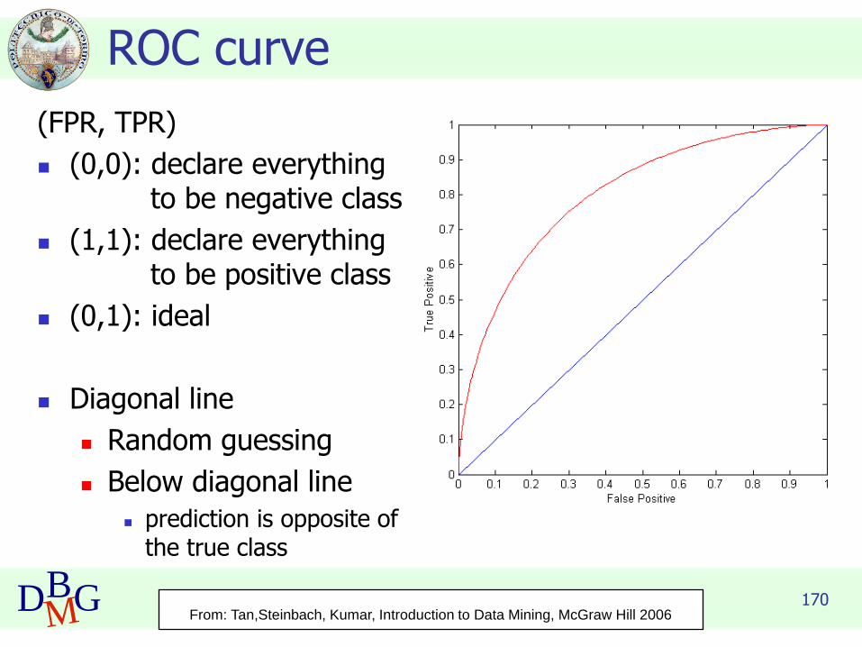
ROC curve
(FPR, TPR)
◼ (0,0): declare everythingto be negative class
◼ (1,1): declare everythingto be positive class
◼ (0,1): ideal
◼ Diagonal line
◼ Random guessing
◼ Below diagonal line
◼ prediction is opposite of the true class
From: Tan,Steinbach, Kumar, Introduction to Data Mining, McGraw Hill 2006

171DBMG
How to build a ROC curve
Instance P(+|A) True Class
1 0.95 +
2 0.93 +
3 0.87 -
4 0.85 -
5 0.85 -
6 0.85 +
7 0.76 -
8 0.53 +
9 0.43 -
10 0.25 +
From: Tan,Steinbach, Kumar, Introduction to Data Mining, McGraw Hill 2006
◼ Use classifier that produces posterior probability for each test instance P(+|A)
◼ Sort the instances according to P(+|A) in decreasing order
◼ Apply threshold at each unique value of P(+|A)
◼ Count the number of TP, FP, TN, FN at each threshold
◼ TP rate
TPR = TP/(TP+FN)
◼ FP rate
FPR = FP/(FP + TN)

172DBMG
How to build a ROC curveClass + - + - - - + - + +
P 0.25 0.43 0.53 0.76 0.85 0.85 0.85 0.87 0.93 0.95 1.00
TP 5 4 4 3 3 3 3 2 2 1 0
FP 5 5 4 4 3 2 1 1 0 0 0
TN 0 0 1 1 2 3 4 4 5 5 5
FN 0 1 1 2 2 2 2 3 3 4 5
TPR 1 0.8 0.8 0.6 0.6 0.6 0.6 0.4 0.4 0.2 0
FPR 1 1 0.8 0.8 0.6 0.4 0.2 0.2 0 0 0
P(+|A)
ROC Curve
From: Tan,Steinbach, Kumar, Introduction to Data Mining, McGraw Hill 2006

173DBMG
Using ROC for Model Comparison
From: Tan,Steinbach, Kumar, Introduction to Data Mining, McGraw Hill 2006
◼ No model consistently outperforms the other
◼ M1 is better for small FPR
◼ M2 is better for large FPR
◼ Area under ROC curve
◼ Ideal
Area = 1.0
◼ Random guess
Area = 0.5