Classification: Logistic Regression

Hung-yi Lee

李宏毅

有關分組

•作業以個人為單位繳交

•期末專題才需要分組

•找不到組員也沒有關係，期末專題公告後找不到組員的同學助教會幫忙湊對

Step 1: Function Set

𝜎 𝑧 =1

1 + 𝑒𝑥𝑝 −𝑧

𝑧 = 𝑤 ∙ 𝑥 + 𝑏

𝑃𝑤,𝑏 𝐶1|𝑥 = 𝜎 𝑧 z

z

Function set: Including all different w and b

=

𝑖

𝑤𝑖𝑥𝑖 + 𝑏

𝑃𝑤,𝑏 𝐶1|𝑥 ≥ 0.5

𝑃𝑤,𝑏 𝐶1|𝑥 < 0.5

class 1

class 2

z

z

0

0

bxwzi

ii

Step 1: Function Set

z

1w

iw

Iw

…

1x

ix

Ix

b

z

…

……

𝑃𝑤,𝑏 𝐶1|𝑥

z

z

ze

z

1

1

Sigmoid Function

Step 2: Goodness of a Function

𝑥1 𝑥2 𝑥3 𝑥𝑁……

𝐶1 𝐶1 𝐶2 𝐶1

TrainingData

Given a set of w and b, what is its probability of generating the data?

𝐿 𝑤, 𝑏 = 𝑓𝑤,𝑏 𝑥1 𝑓𝑤,𝑏 𝑥2 1 − 𝑓𝑤,𝑏 𝑥3 ⋯𝑓𝑤,𝑏 𝑥𝑁

The most likely w* and b* is the one with the largest 𝐿 𝑤, 𝑏 .

Assume the data is generated based on 𝑓𝑤,𝑏 𝑥 = 𝑃𝑤,𝑏 𝐶1|𝑥

𝑤∗, 𝑏∗ = 𝑎𝑟𝑔max𝑤,𝑏

𝐿 𝑤, 𝑏

𝐿 𝑤, 𝑏 = 𝑓𝑤,𝑏 𝑥1 𝑓𝑤,𝑏 𝑥2 1 − 𝑓𝑤,𝑏 𝑥3 ⋯

𝑤∗, 𝑏∗ = 𝑎𝑟𝑔max𝑤,𝑏

𝐿 𝑤, 𝑏 𝑤∗, 𝑏∗ = 𝑎𝑟𝑔min𝑤,𝑏

−𝑙𝑛𝐿 𝑤, 𝑏

−𝑙𝑛𝐿 𝑤, 𝑏

= −𝑙𝑛𝑓𝑤,𝑏 𝑥1

−𝑙𝑛𝑓𝑤,𝑏 𝑥2

……

−𝑙𝑛 1 − 𝑓𝑤,𝑏 𝑥3

ො𝑦𝑛: 1 for class 1, 0 for class 2

− ො𝑦1𝑙𝑛𝑓 𝑥1 + 1 − ො𝑦1 𝑙𝑛 1 − 𝑓 𝑥1

− ො𝑦3𝑙𝑛𝑓 𝑥3 + 1 − ො𝑦3 𝑙𝑛 1 − 𝑓 𝑥3

=

𝑥1 𝑥2 𝑥3……

𝐶1 𝐶1 𝐶2

𝑥1 𝑥2 𝑥3……

ො𝑦1 = 1 ො𝑦2 = 1 ො𝑦3 = 0

− ො𝑦2𝑙𝑛𝑓 𝑥2 + 1 − ො𝑦2 𝑙𝑛 1 − 𝑓 𝑥2

1

1

0

0

10

Step 2: Goodness of a Function

𝐿 𝑤, 𝑏 = 𝑓𝑤,𝑏 𝑥1 𝑓𝑤,𝑏 𝑥2 1 − 𝑓𝑤,𝑏 𝑥3 ⋯𝑓𝑤,𝑏 𝑥𝑁

−𝑙𝑛𝐿 𝑤, 𝑏 = 𝑙𝑛𝑓𝑤,𝑏 𝑥1 + 𝑙𝑛𝑓𝑤,𝑏 𝑥2 + 𝑙𝑛 1 − 𝑓𝑤,𝑏 𝑥3 ⋯

=

𝑛

− ො𝑦𝑛𝑙𝑛𝑓𝑤,𝑏 𝑥𝑛 + 1 − ො𝑦𝑛 𝑙𝑛 1 − 𝑓𝑤,𝑏 𝑥𝑛

ො𝑦𝑛: 1 for class 1, 0 for class 2

Cross entropy between two Bernoulli distribution

Distribution p:

p 𝑥 = 1 = ො𝑦𝑛

p 𝑥 = 0 = 1 − ො𝑦𝑛

Distribution q:

q 𝑥 = 1 = 𝑓 𝑥𝑛

q 𝑥 = 0 = 1 − 𝑓 𝑥𝑛

𝐻 𝑝, 𝑞 = −

𝑥

𝑝 𝑥 𝑙𝑛 𝑞 𝑥

cross entropy

Step 2: Goodness of a Function

𝐿 𝑤, 𝑏 = 𝑓𝑤,𝑏 𝑥1 𝑓𝑤,𝑏 𝑥2 1 − 𝑓𝑤,𝑏 𝑥3 ⋯𝑓𝑤,𝑏 𝑥𝑁

−𝑙𝑛𝐿 𝑤, 𝑏 = 𝑙𝑛𝑓𝑤,𝑏 𝑥1 + 𝑙𝑛𝑓𝑤,𝑏 𝑥2 + 𝑙𝑛 1 − 𝑓𝑤,𝑏 𝑥3 ⋯

=

𝑛

− ො𝑦𝑛𝑙𝑛𝑓𝑤,𝑏 𝑥𝑛 + 1 − ො𝑦𝑛 𝑙𝑛 1 − 𝑓𝑤,𝑏 𝑥𝑛

ො𝑦𝑛: 1 for class 1, 0 for class 2

Cross entropy between two Bernoulli distribution

𝑓 𝑥𝑛

1 − 𝑓 𝑥𝑛1.0

Ground Truth ො𝑦𝑛 = 1

cross entropy

minimize

0.0

Step 3: Find the best function

𝜕𝑤𝑖

−𝑙𝑛𝐿 𝑤, 𝑏 =

𝑛

− ො𝑦𝑛𝑙𝑛𝑓𝑤,𝑏 𝑥𝑛 + 1 − ො𝑦𝑛 𝑙𝑛 1 − 𝑓𝑤,𝑏 𝑥𝑛

𝜕𝑤𝑖 𝜕𝑤𝑖

𝑓𝑤,𝑏 𝑥 = 𝜎 𝑧

= Τ1 1 + 𝑒𝑥𝑝 −𝑧𝑧 = 𝑤 ∙ 𝑥 + 𝑏 =

𝑖

𝑤𝑖𝑥𝑖 + 𝑏

𝜕𝑙𝑛𝑓𝑤,𝑏 𝑥

𝜕𝑤𝑖=𝜕𝑙𝑛𝑓𝑤,𝑏 𝑥

𝜕𝑧

𝜕𝑧

𝜕𝑤𝑖

𝜕𝑧

𝜕𝑤𝑖= 𝑥𝑖

𝜕𝑙𝑛𝜎 𝑧

𝜕𝑧=

1

𝜎 𝑧

𝜕𝜎 𝑧

𝜕𝑧=

1

𝜎 𝑧𝜎 𝑧 1 − 𝜎 𝑧

1 − 𝑓𝑤,𝑏 𝑥𝑛 𝑥𝑖𝑛

𝜎 𝑧

𝜕𝜎 𝑧

𝜕𝑧

Step 3: Find the best function

𝜕𝑤𝑖

−𝑙𝑛𝐿 𝑤, 𝑏 =

𝑛

− ො𝑦𝑛𝑙𝑛𝑓𝑤,𝑏 𝑥𝑛 + 1 − ො𝑦𝑛 𝑙𝑛 1 − 𝑓𝑤,𝑏 𝑥𝑛

𝜕𝑤𝑖 𝜕𝑤𝑖

𝑓𝑤,𝑏 𝑥 = 𝜎 𝑧

= Τ1 1 + 𝑒𝑥𝑝 −𝑧𝑧 = 𝑤 ∙ 𝑥 + 𝑏 =

𝑖

𝑤𝑖𝑥𝑖 + 𝑏

𝜕𝑙𝑛 1 − 𝑓𝑤,𝑏 𝑥

𝜕𝑤𝑖=𝜕𝑙𝑛 1 − 𝑓𝑤,𝑏 𝑥

𝜕𝑧

𝜕𝑧

𝜕𝑤𝑖

𝜕𝑧

𝜕𝑤𝑖= 𝑥𝑖

𝜕𝑙𝑛 1 − 𝜎 𝑧

𝜕𝑧= −

1

1 − 𝜎 𝑧

𝜕𝜎 𝑧

𝜕𝑧= −

1

1 − 𝜎 𝑧𝜎 𝑧 1 − 𝜎 𝑧

−𝑓𝑤,𝑏 𝑥𝑛 𝑥𝑖𝑛1 − 𝑓𝑤,𝑏 𝑥𝑛 𝑥𝑖

𝑛

Step 3: Find the best function

𝜕𝑤𝑖

−𝑙𝑛𝐿 𝑤, 𝑏 =

𝑛

− ො𝑦𝑛𝑙𝑛𝑓𝑤,𝑏 𝑥𝑛 + 1 − ො𝑦𝑛 𝑙𝑛 1 − 𝑓𝑤,𝑏 𝑥𝑛

𝜕𝑤𝑖 𝜕𝑤𝑖

=

𝑛

− ො𝑦𝑛 1 − 𝑓𝑤,𝑏 𝑥𝑛 𝑥𝑖𝑛 − 1 − ො𝑦𝑛 𝑓𝑤,𝑏 𝑥𝑛 𝑥𝑖

𝑛

=

𝑛

− ො𝑦𝑛 − ො𝑦𝑛𝑓𝑤,𝑏 𝑥𝑛 − 𝑓𝑤,𝑏 𝑥𝑛 + ො𝑦𝑛𝑓𝑤,𝑏 𝑥𝑛 𝑥𝑖𝑛

=

𝑛

− ො𝑦𝑛 − 𝑓𝑤,𝑏 𝑥𝑛 𝑥𝑖𝑛

𝑤𝑖 ← 𝑤𝑖 − 𝜂

𝑛

− ො𝑦𝑛 − 𝑓𝑤,𝑏 𝑥𝑛 𝑥𝑖𝑛

Larger difference, larger update

−𝑓𝑤,𝑏 𝑥𝑛 𝑥𝑖𝑛1 − 𝑓𝑤,𝑏 𝑥𝑛 𝑥𝑖

𝑛

Logistic Regression + Square Error

𝑓𝑤,𝑏 𝑥 = 𝜎

𝑖

𝑤𝑖𝑥𝑖 + 𝑏

Training data: 𝑥𝑛, ො𝑦𝑛 , ො𝑦𝑛: 1 for class 1, 0 for class 2

𝐿 𝑓 =1

2

𝑛

𝑓𝑤,𝑏 𝑥𝑛 − ො𝑦𝑛2

Step 1:

Step 2:

= 2 𝑓𝑤,𝑏 𝑥 − ො𝑦𝜕𝑓𝑤,𝑏 𝑥

𝜕𝑧

Step 3:

= 2 𝑓𝑤,𝑏 𝑥 − ො𝑦 𝑓𝑤,𝑏 𝑥 1 − 𝑓𝑤,𝑏 𝑥 𝑥𝑖

ො𝑦𝑛 = 1 If 𝑓𝑤,𝑏 𝑥𝑛 = 1 Τ𝜕𝐿 𝜕𝑤𝑖 = 0

If 𝑓𝑤,𝑏 𝑥𝑛 = 0 Τ𝜕𝐿 𝜕𝑤𝑖 = 0(far from target)

(close to target)

𝜕 (𝑓𝑤,𝑏(𝑥)−ො𝑦)2

𝜕𝑤𝑖

𝜕𝑧

𝜕𝑤𝑖

Logistic Regression + Square Error

ො𝑦𝑛 = 0 If 𝑓𝑤,𝑏 𝑥𝑛 = 1 Τ𝜕𝐿 𝜕𝑤𝑖 = 0

If 𝑓𝑤,𝑏 𝑥𝑛 = 0 Τ𝜕𝐿 𝜕𝑤𝑖 = 0(close to target)

(far from target)

𝑓𝑤,𝑏 𝑥 = 𝜎

𝑖

𝑤𝑖𝑥𝑖 + 𝑏

Training data: 𝑥𝑛, ො𝑦𝑛 , ො𝑦𝑛: 1 for class 1, 0 for class 2

𝐿 𝑓 =1

2

𝑛

𝑓𝑤,𝑏 𝑥𝑛 − ො𝑦𝑛2

Step 1:

Step 2:

Step 3:= 2 𝑓𝑤,𝑏 𝑥 − ො𝑦

𝜕𝑓𝑤,𝑏 𝑥

𝜕𝑧

= 2 𝑓𝑤,𝑏 𝑥 − ො𝑦 𝑓𝑤,𝑏 𝑥 1 − 𝑓𝑤,𝑏 𝑥 𝑥𝑖

𝜕 (𝑓𝑤,𝑏(𝑥)−ො𝑦)2

𝜕𝑤𝑖

𝜕𝑧

𝜕𝑤𝑖

Cross Entropy v.s. Square Error

Total Loss

w1w2

Cross Entropy

SquareError

http://jmlr.org/proceedings/papers/v9/glorot10a/glorot10a.pdf

Logistic Regression Linear Regression

𝑓𝑤,𝑏 𝑥 =

𝑖

𝑤𝑖𝑥𝑖 + 𝑏Step 1: 𝑓𝑤,𝑏 𝑥 = 𝜎

𝑖

𝑤𝑖𝑥𝑖 + 𝑏

Step 2:

Step 3:

Output: between 0 and 1 Output: any value

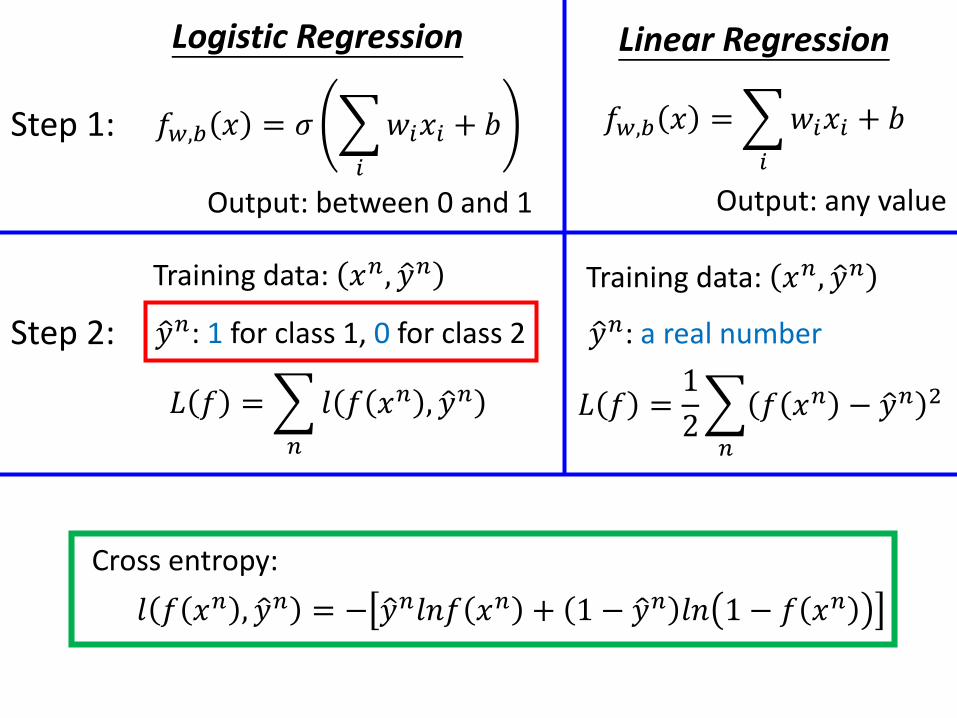
Logistic Regression Linear Regression

Step 1:

Step 2:

Output: between 0 and 1 Output: any value

𝐿 𝑓 =

𝑛

𝑙 𝑓 𝑥𝑛 , ො𝑦𝑛

ො𝑦𝑛: 1 for class 1, 0 for class 2

Training data: 𝑥𝑛, ො𝑦𝑛

𝐿 𝑓 =1

2

𝑛

𝑓 𝑥𝑛 − ො𝑦𝑛 2

Training data: 𝑥𝑛, ො𝑦𝑛

ො𝑦𝑛: a real number

𝑙 𝑓 𝑥𝑛 , ො𝑦𝑛 = − ො𝑦𝑛𝑙𝑛𝑓 𝑥𝑛 + 1 − ො𝑦𝑛 𝑙𝑛 1 − 𝑓 𝑥𝑛Cross entropy:

𝑓𝑤,𝑏 𝑥 =

𝑖

𝑤𝑖𝑥𝑖 + 𝑏𝑓𝑤,𝑏 𝑥 = 𝜎

𝑖

𝑤𝑖𝑥𝑖 + 𝑏

Logistic Regression Linear Regression

Step 1:

Step 2:

Output: between 0 and 1 Output: any value

𝐿 𝑓 =

𝑛

𝑙 𝑓 𝑥𝑛 , ො𝑦𝑛

ො𝑦𝑛: 1 for class 1, 0 for class 2

Training data: 𝑥𝑛, ො𝑦𝑛

𝐿 𝑓 =1

2

𝑛

𝑓 𝑥𝑛 − ො𝑦𝑛 2

Training data: 𝑥𝑛, ො𝑦𝑛

ො𝑦𝑛: a real number

𝑓𝑤,𝑏 𝑥 =

𝑖

𝑤𝑖𝑥𝑖 + 𝑏𝑓𝑤,𝑏 𝑥 = 𝜎

𝑖

𝑤𝑖𝑥𝑖 + 𝑏

Step 3:

𝑤𝑖 ← 𝑤𝑖 − 𝜂

𝑛

− ො𝑦𝑛 − 𝑓𝑤,𝑏 𝑥𝑛 𝑥𝑖𝑛

𝑤𝑖 ← 𝑤𝑖 − 𝜂

𝑛

− ො𝑦𝑛 − 𝑓𝑤,𝑏 𝑥𝑛 𝑥𝑖𝑛Logistic regression:

Linear regression:

Discriminative v.s. Generative

𝑃 𝐶1|𝑥 = 𝜎 𝑤 ∙ 𝑥 + 𝑏

directly find w and b

𝑤𝑇 = 𝜇1 − 𝜇2 𝑇Σ−1

Find 𝜇1, 𝜇2, Σ−1

𝑏 = −1

2𝜇1 𝑇 Σ1 −1𝜇1

+1

2𝜇2 𝑇 Σ2 −1𝜇2 + 𝑙𝑛

𝑁1𝑁2

The same model (function set), but different function may be selected by the same training data.

Will we obtain the same set of w and b?

Generative v.s. Discriminative

All: hp, att, sp att, de, sp de, speed

73% accuracy 79% accuracy

Generative Discriminative

• Example

Generative v.s. Discriminative

Class 2Class 1

1

1

1

0

0

1

0

0X 4 X 4 X 4

Class 2 Class 2

Training Data

1

1

TestingData

Class 1?Class 2?

How about Naïve Bayes?

𝑃 𝑥|𝐶𝑖 = 𝑃 𝑥1|𝐶𝑖 𝑃 𝑥2|𝐶𝑖

• Example

Generative v.s. Discriminative

Class 2Class 1

1

1

1

0

0

1

0

0X 4 X 4 X 4

Class 2 Class 2

Training Data

𝑃 𝐶1 =1

13

𝑃 𝐶2 =12

13

𝑃 𝑥1 = 1|𝐶1 = 1 𝑃 𝑥2 = 1|𝐶1 = 1

𝑃 𝑥1 = 1|𝐶2 =1

3 𝑃 𝑥2 = 1|𝐶2 =1

3

𝑃 𝐶1 =1

13

𝑃 𝐶2 =12

13

𝑃 𝑥1 = 1|𝐶1 = 1 𝑃 𝑥2 = 1|𝐶1 = 1

𝑃 𝑥1 = 1|𝐶2 =1

3 𝑃 𝑥2 = 1|𝐶2 =1

3

1

1

TestingData

=𝑃 𝑥|𝐶1 𝑃 𝐶1

𝑃 𝑥|𝐶1 𝑃 𝐶1 + 𝑃 𝑥|𝐶2 𝑃 𝐶2𝑃 𝐶1|𝑥

1

131 × 1

1

131 × 1

12

13

1

3×1

3

<0.5

Class 2Class 1

1

1

1

0

0

1

0

0X 4 X 4 X 4

Class 2 Class 2

Training Data

Generative v.s. Discriminative

• Usually people believe discriminative model is better

• Benefit of generative model

• With the assumption of probability distribution

• less training data is needed

• more robust to the noise

• Priors and class-dependent probabilities can be estimated from different sources.

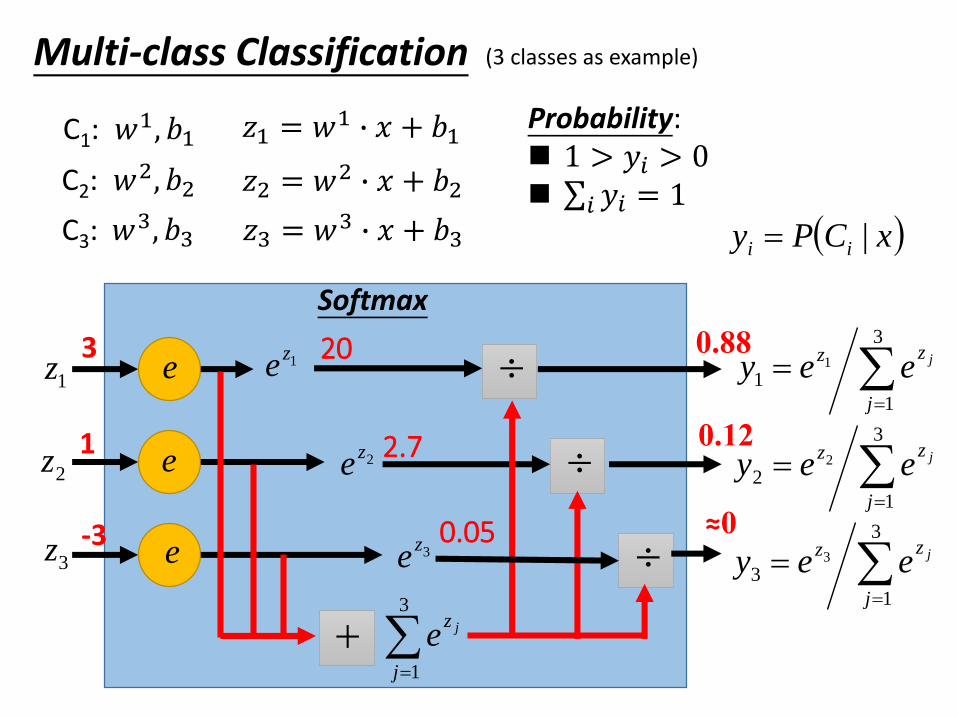
Multi-class Classification

C1:

C2:

C3:

𝑤1, 𝑏1

𝑤2, 𝑏2

𝑤3, 𝑏3

𝑧1 = 𝑤1 ∙ 𝑥 + 𝑏1

𝑧2 = 𝑤2 ∙ 𝑥 + 𝑏2

𝑧3 = 𝑤3 ∙ 𝑥 + 𝑏3

(3 classes as example)

1z

2z

3z

Softmax

e

e

e

1ze

2ze

3ze

3

1

11

j

zz jeey

3

1j

z je

3

-3

1 2.7

20

0.05

0.88

0.12

≈0

3

1

22

j

zz jeey

3

1

33

j

zz jeey

Probability: 1 > 𝑦𝑖 > 0 σ𝑖 𝑦𝑖 = 1

xCPy ii |

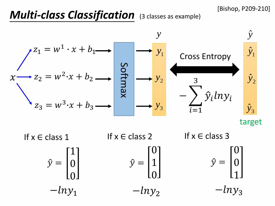
Multi-class Classification (3 classes as example)

ො𝑦 =100

Softm

ax

1y

2y

3y

𝑧1 = 𝑤1 ∙ 𝑥 + 𝑏1

𝑧2 = 𝑤2∙𝑥 + 𝑏2

𝑧3 = 𝑤3∙𝑥 + 𝑏3

𝑥

y

1y

y

2y

3y

Cross Entropy

−

𝑖=1

3

ො𝑦𝑖𝑙𝑛𝑦𝑖

ො𝑦 =

010

ො𝑦 =001

If x ∈ class 1 If x ∈ class 2 If x ∈ class 3

target

[Bishop, P209-210]

−𝑙𝑛𝑦1 −𝑙𝑛𝑦2 −𝑙𝑛𝑦3

1x

2x

Limitation of Logistic Regression

Input FeatureLabel

x1 x2

0 0 Class 2

0 1 Class 1

1 0 Class 1

1 1 Class 2

yz

1w

2w

1x

2xb

5.02

5.01

yClass

yClassbxwxwz 2211

z ≥ 0

z ≥ 0

z < 0

z < 0

Can we?

(𝑧 ≥ 0)

(𝑧 < 0)

Limitation of Logistic Regression

• Feature transformation

1x

2x

00

11

01

01

𝑥1𝑥2

𝑥1′

𝑥2′

𝑥1′ : distance to

00

𝑥2′ : distance to

11

0

2

11

𝑥1′

𝑥2′

20

Not always easy ….. domain knowledge can be helpful

Limitation of Logistic Regression

• Cascading logistic regression models

1z

2z

1x

2x

yz

(ignore bias in this figure)

𝑥1′

𝑥2′

Feature Transformation Classification

1x

2x

𝑥2′=0.27

𝑥2′=0.73𝑥2

′=0.27

𝑥2′=0.05

𝑥1′=0.27

1x

2x

𝑥1′=0.27

𝑥1′=0.05

𝑥1′=0.73

2z

2x

2x

𝑥1′

𝑥2′

2z

2

-2

2

-2

-1

-1

yz

1w

2w

(0.27, 0.27)

(0.73, 0.05)

(0.05,0.73)

𝑥1′

𝑥2′

𝑥1′

𝑥2′

1x

2x

𝑥2′=0.27

𝑥2′=0.73𝑥2

′=0.27

𝑥2′=0.05

𝑥1′=0.27

2x

2x

𝑥1′=0.27

𝑥1′=0.05

𝑥1′=0.73

b

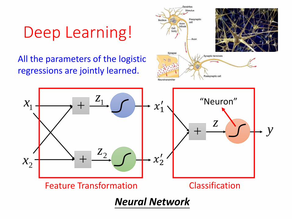
Deep Learning!

1z

2z

1x

2x

yz

𝑥1′

𝑥2′

Feature Transformation Classification

“Neuron”

Neural Network

All the parameters of the logistic regressions are jointly learned.

Reference

• Bishop: Chapter 4.3

Acknowledgement

•感謝林恩妤發現投影片上的錯誤

Appendix

• Step 1. Function Set (Model)

• Step 2. Goodness of a function

• Step 3. Find the best function: gradient descent

Three Steps

𝑥 If 𝑃 𝐶1|𝑥 > 0.5, output: y = class 1

Otherwise, output: y = class 2

𝑃 𝐶1|𝑥 = 𝜎 𝑤 ∙ 𝑥 + 𝑏

w and b are related to 𝑁1, 𝑁2, 𝜇1, 𝜇2, Σ

𝐿 𝑓 =

𝑛

𝛿 𝑓 𝑥𝑛 ≠ ො𝑦𝑛 𝐿 𝑓 =

𝑛

𝑙 𝑓 𝑥𝑛 ≠ ො𝑦𝑛

𝑥1 𝑥2 𝑥3……

ො𝑦1 ො𝑦2 ො𝑦3

ො𝑦𝑛 = 𝑐𝑙𝑎𝑠𝑠 1, 𝑐𝑙𝑎𝑠𝑠 2

𝑥𝑛

ො𝑦𝑛

𝑦

feature class

𝐿 𝑓 =

𝑛

𝛿 𝑓 𝑥𝑛 ≠ ො𝑦𝑛

Step 2: Loss function

ො𝑦𝑛𝑧𝑛

Ideal loss

Ideal loss:

𝐿 𝑓 =

𝑛

𝑙 𝑓 𝑥𝑛 , ො𝑦𝑛

Approximation:

𝛿 𝑓 𝑥𝑛 ≠ ො𝑦𝑛

𝑓𝑤,𝑏 𝑥 =≥ class 1

class 2

z

z

0

0<

+1

-1

𝑙 ∗ is the upper bound of 𝛿 ∗

0 or 1

Step 2: Loss function 𝑙 𝑓 𝑥𝑛 , ො𝑦𝑛 : cross entropy

𝑓 𝑥𝑛ො𝑦𝑛 = +1

ො𝑦𝑛 = −1 1 − 𝑓 𝑥𝑛 1.0Ground

Truthcross entropy

If ො𝑦𝑛 = +1:

𝑙 𝑓 𝑥𝑛 , ො𝑦𝑛 = −ln𝑓 𝑥𝑛

If ො𝑦𝑛 = −1:

𝑙 𝑓 𝑥𝑛 , ො𝑦𝑛 = −ln 1 − 𝑓 𝑥𝑛

= −ln𝜎 𝑧𝑛 = −ln1

1 + 𝑒𝑥𝑝 −𝑧𝑛

= ln 1 + 𝑒𝑥𝑝 −𝑧𝑛 = ln 1 + 𝑒𝑥𝑝 −ො𝑦𝑛𝑧𝑛

= −ln 1 − 𝜎 𝑥𝑛 = −ln𝑒𝑥𝑝 −𝑧𝑛

1 + 𝑒𝑥𝑝 −𝑧𝑛= −ln

1

1 + 𝑒𝑥𝑝 𝑧𝑛

= ln 1 + 𝑒𝑥𝑝 𝑧𝑛 = ln 1 + 𝑒𝑥𝑝 −ො𝑦𝑛𝑧𝑛

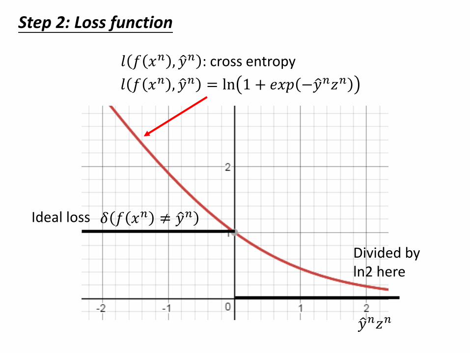
Step 2: Loss function

𝑙 𝑓 𝑥𝑛 , ො𝑦𝑛 = ln 1 + 𝑒𝑥𝑝 −ො𝑦𝑛𝑧𝑛

Ideal loss 𝛿 𝑓 𝑥𝑛 ≠ ො𝑦𝑛

ො𝑦𝑛𝑧𝑛

Divided by ln2 here

𝑙 𝑓 𝑥𝑛 , ො𝑦𝑛 : cross entropy