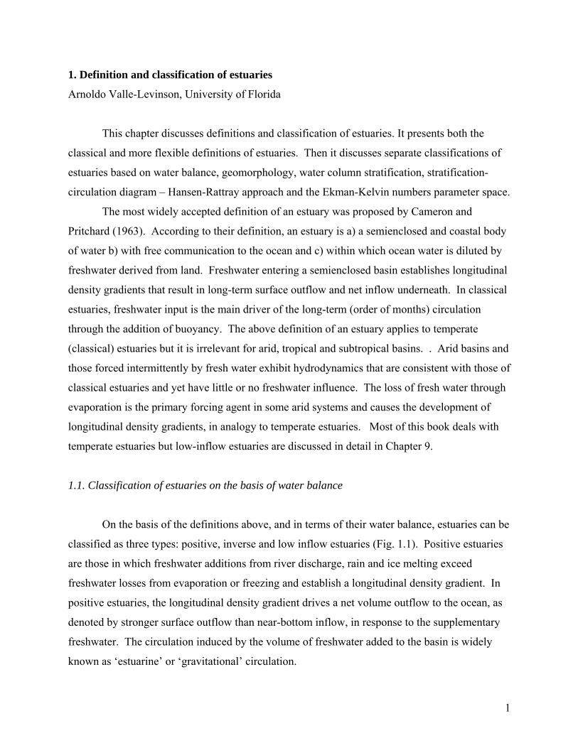
1. Definition and classification of estuaries

Arnoldo Valle-Levinson, University of Florida

This chapter discusses definitions and classification of estuaries. It presents both the

classical and more flexible definitions of estuaries. Then it discusses separate classifications of

estuaries based on water balance, geomorphology, water column stratification, stratification-

circulation diagram – Hansen-Rattray approach and the Ekman-Kelvin numbers parameter space.

The most widely accepted definition of an estuary was proposed by Cameron and

Pritchard (1963). According to their definition, an estuary is a) a semienclosed and coastal body

of water b) with free communication to the ocean and c) within which ocean water is diluted by

freshwater derived from land. Freshwater entering a semienclosed basin establishes longitudinal

density gradients that result in long-term surface outflow and net inflow underneath. In classical

estuaries, freshwater input is the main driver of the long-term (order of months) circulation

through the addition of buoyancy. The above definition of an estuary applies to temperate

(classical) estuaries but it is irrelevant for arid, tropical and subtropical basins. . Arid basins and

those forced intermittently by fresh water exhibit hydrodynamics that are consistent with those of

classical estuaries and yet have little or no freshwater influence. The loss of fresh water through

evaporation is the primary forcing agent in some arid systems and causes the development of

longitudinal density gradients, in analogy to temperate estuaries. Most of this book deals with

temperate estuaries but low-inflow estuaries are discussed in detail in Chapter 9.

1.1. Classification of estuaries on the basis of water balance

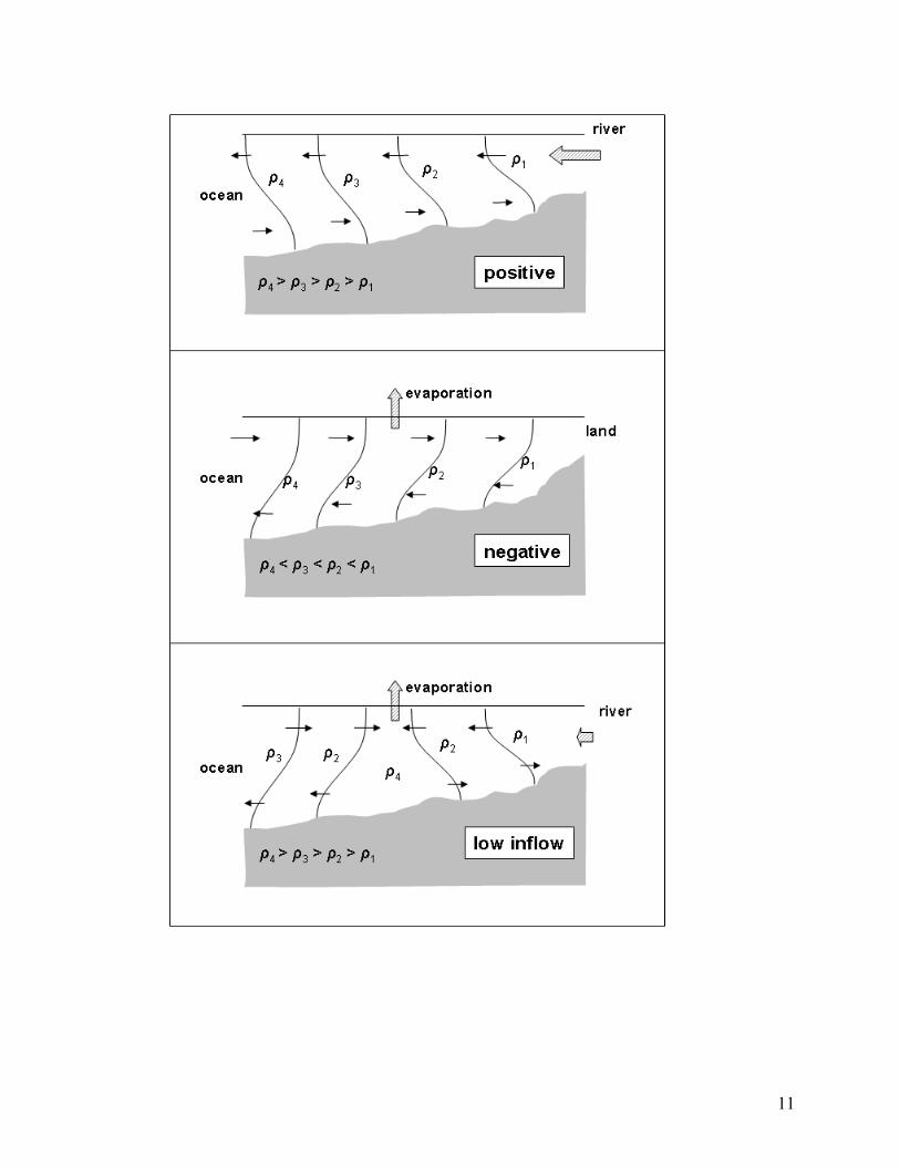
On the basis of the definitions above, and in terms of their water balance, estuaries can be

classified as three types: positive, inverse and low inflow estuaries (Fig. 1.1). Positive estuaries

are those in which freshwater additions from river discharge, rain and ice melting exceed

freshwater losses from evaporation or freezing and establish a longitudinal density gradient. In

positive estuaries, the longitudinal density gradient drives a net volume outflow to the ocean, as

denoted by stronger surface outflow than near-bottom inflow, in response to the supplementary

freshwater. The circulation induced by the volume of freshwater added to the basin is widely

known as ‘estuarine’ or ‘gravitational’ circulation.

1

Inverse estuaries are typically found in arid regions where freshwater losses from

evaporation exceed freshwater additions from precipitation. There is no or scant river discharge

into these systems. They are called inverse, or negative, because the longitudinal density

gradient has the opposite sign to that in positive estuaries, i.e., water density increases landward.

Inverse estuaries exhibit net volume inflows associated with stronger surface inflows than near-

bottom outflows. Water losses related to inverse estuaries make their flushing more sluggish

than positive estuaries. Because of their relatively sluggish flushing, negative estuaries are likely

more prone to water quality problems than positive estuaries.

Low inflow estuaries also occur in regions of high evaporation rates but with a small (of a

few m3/s) influence from river discharge. During the dry and hot season, evaporation processes

may cause a salinity maximum zone (sometimes referred to as salt plug, e.g. Wolanski, 1986)

within these low-inflow estuaries. Seaward of this salinity maximum, the water density

decreases seaward, as in an inverse estuary. Landward of the salinity maximum, water density

decreases as in a positive estuary. Therefore, the zone of maximum salinity acts as a barrier that

precludes the seaward flushing of riverine waters and the landward intrusion of ocean waters.

Because of their weak flushing in the region landward of the salinity maximum, low-inflow

estuaries are also prone to water quality problems.

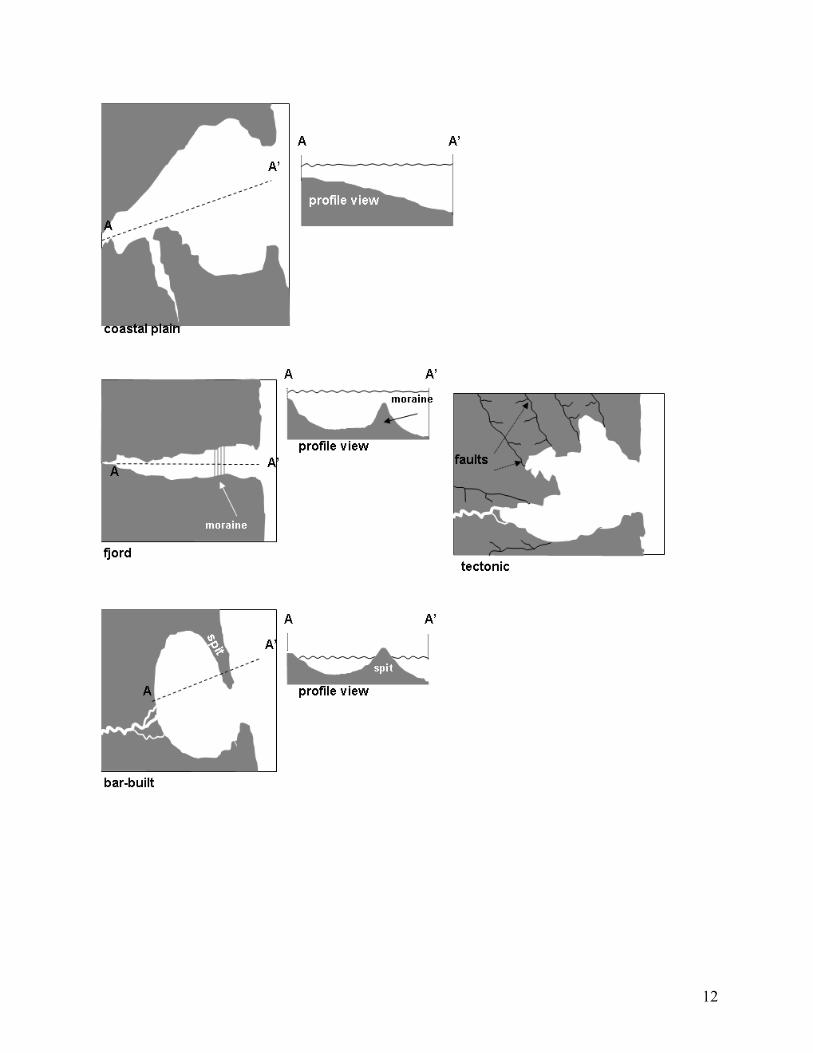
1.2. Classification of estuaries on the basis of geomorphology

Estuaries may be classified according to their geomorphology in coastal plain, fjord, bar-

built and tectonic (Fig. 1.2; Pritchard, 1952). Coastal plain estuaries, also called drowned river-

valleys, are those that were formed as a result of the Pleistocene increase in sea level, starting

~15,000 years ago. Originally rivers, these estuaries formed during flooding over several

millennia by rising sea levels. Their shape resembles that of present-day rivers, although much

wider. They are typically wide (order of several kilometers) and shallow (order 10 m) with large

width/depth aspect ratios. Examples of these systems are Chesapeake Bay and Delaware Bay on

the eastern coast of the United States.

Fjords are associated with high latitudes where glacial activity is intense. They are

characterized by an elongated, deep channel with a sill. The sill is related to a moraine of either

a currently active glacier or an extinct glacier. In the sense of the glacier activity, it could be said

2

that there are riverine and glacial fjords. Riverine fjords are related to extinct glaciers and their

main source of buoyancy comes from river inputs. They are usually found equatorward of

glacial fjords. Glacial fjords are found in high latitudes, poleward of riverine fjords. They are

related to active glaciers and their main source of buoyancy is derived from melting of the

glacier and of snow and ice in mountains nearby. Fjords are deep (several hundred meters) and

narrow (several hundreds of meters) and have low width/depth aspect ratios with steep side

walls. Fjords are found in Greenland, Alaska, British Columbia, Norway, New Zealand,

Antarctica and Chile.

Bar-built estuaries, originally embayments, became semi-enclosed because of littoral drift

causing the formation of a sand bar or spit between the coast and the ocean. Some of these bars

are joined to one of the headlands of a former embayment and display one small inlet (few

hundreds of meters) where the estuary communicates with the ocean. Some other sand bars may

be detached from the coast and represent islands that result in two or more inlets that allow

communication between the estuary and the ocean. In some additional cases, sand bars were

formed by rising sea level. Examples of bar-built estuaries abound in subtropical regions of the

Americas (e.g. North Carolina, Florida, northern Mexico) and southern Portugal.

Tectonic estuaries were formed by earthquakes or by Earth’s crust fractures and creases

that generated faults in regions adjacent to the ocean. Faults cause part of the crust to sink,

forming then a hollow basin. An estuary is formed when the basin is filled in by the ocean.

Examples of this type of estuary are San Francisco Bay in the United States, Manukau Harbour

in New Zealand, some Rías in Spain and Guaymas Bay in Mexico.

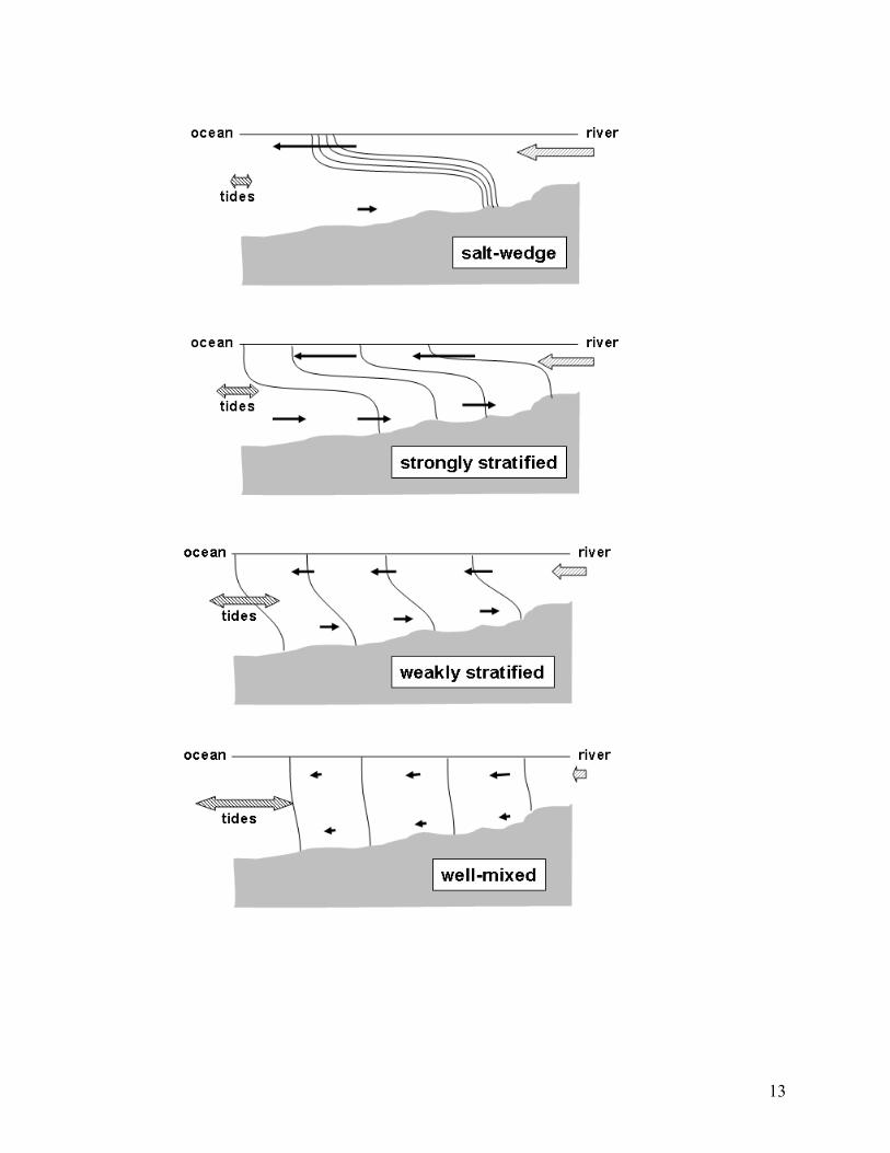
1.3. Classification of estuaries on the basis of vertical structure of salinity

According to water column stratification or salinity vertical structure, estuaries can be

classified as salt wedge, strongly stratified, weakly stratified or vertically mixed (Pritchard,

1955; Cameron & Pritchard, 1963). This classification considers the competition between

buoyancy forcing from river discharge and mixing from tidal forcing (Fig. 1.3). Mixing from

tidal forcing is proportional to the volume of oceanic water entering the estuary during every

tidal cycle, which is also known as the tidal prism. Large river discharge and weak tidal forcing

results in salt wedge estuaries such as the Mississippi (USA), Rio de la Plata (Argentina), Vellar

3

(India), Ebro (Spain), Pánuco (Mexico), and Itajaí-Açu (Brazil). These systems are strongly

stratified during flood tides, when the ocean water intrudes in a wedge shape. Some of these

systems lose their salt wedge nature during dry periods. Typical tidally averaged salinity profiles

exhibit a sharp pycnocline (or halocline) with mean flows dominated by outflow throughout

most of the water column with weak inflow in a near-bottom layer. The mean flow pattern

results from relatively weak mixing between the inflowing ocean water and the river water.

Moderate to large river discharge and weak to moderate tidal forcing result in strongly

stratified estuaries (Fig. 1.3). These estuaries have similar stratification to salt wedge estuaries

but the stratification remains strong throughout the tidal cycle as in fjords and other deep

(typically >20 m deep) estuaries. The tidally averaged salinity profiles have a well-developed

pycnocline with weak vertical variations above and below the pycnocline. The mean tidal flow

exhibits well established outflows and inflows, but the inflows are weak because of weak mixing

with fresh water and weak horizontal density gradients.

Weakly stratified or partially mixed estuaries result from moderate to strong tidal forcing

and weak to moderate river discharge. Many temperate estuaries, such as Chesapeake Bay,

Delware Bay and James River (all in eastern United States) fit into this category. The mean

salinity profile either has a weak pycnocline or continuous stratification from surface to bottom,

except near the bottom mixed layer. The mean exchange flow is most vigorous (when compared

to other types of estuaries) because of the mixing between riverine and oceanic waters.

Strong tidal forcing and weak river discharge result in vertically mixed estuaries. Mean

salinity profiles in mixed estuaries are practically uniform and mean flows are unidirectional

with depth. In wide (and shallow) estuaries, inflows may develop on one side across the estuary

and outflow on the other side, especially during the dry season. Parts of the lower Chesapeake

Bay may exhibit this behavior in early autumn. In narrow well-mixed estuaries, inflow of

salinity may only occur during the flood tide because the mean flow will be seaward. Examples

of this type of estuary are scarce because under well-mixed conditions, the mean (as in the tidally

averaged sense) flow will most likely be driven by wind or tidal forcing (e.g. Chapter 6).

It is essential to keep in mind that many systems may change from one type to the other

in consecutive tidal cycles or from month to month or from season to season or from one

location to the other inside the same estuary. For instance, the Hudson River, in the eastern

United States, changes from highly stratified during neap tides to weakly stratified during spring

4

tides. The Columbia River, in western United States, may be strongly stratified under weak

discharge conditions and similar to a salt-wedge estuary during high discharge conditions.

1.4. Classification of estuaries on the basis of hydrodynamics

A widely accepted classification of estuaries was proposed by Hansen and Rattray (1966)

on the basis of estuarine hydrodynamics. It is best to review this classification after acquiring a

basic understanding of estuarine hydrodynamics, e.g. after Chapter 6 of this text. This

classification is anchored in two hydrodynamic non-dimensional parameters: a) the circulation

parameter and b) the stratification parameter. These parameters refer to tidally averaged and

cross-sectionally averaged variables. The circulation parameter is the ratio of near-surface flow

speed us to sectionally averaged flow Uf. The near-surface flow speed is typically related to the

river discharge and, for the sake of argument, of order 0.1 m/s. The depth-averaged flow Uf is

typically very small, tending to zero, in estuaries of vigorous water exchange because there will

be as much net outflow as net inflow. In estuaries with weak net inflow, such as well mixed and

salt-wedge systems, the depth-averaged flow will be similar in magnitude to the surface outflow.

Therefore, the circulation parameter is >10 in estuaries with vigorous gravitational circulation

and close to 1 in estuaries with unidirectional net outflow. In general, the greater the circulation

parameter, the stronger the gravitational circulation.

The other non-dimensional parameter, the stratification parameter, is the ratio of the top-

to-bottom salinity difference ∂S to the mean salinity over an estuarine cross-section S0. A ratio

of one indicates that the salinity stratification (or top-to-bottom difference) is as large as the

sectional mean salinity. For instance if an estuary shows a sectional mean salinity of 20, for it to

exhibit a stratification parameter of one it must have a very large stratification (of 20). In

general, estuaries will most often have stratification parameters < 1. The weaker the water

column stratification, the smaller the stratification parameter will be.

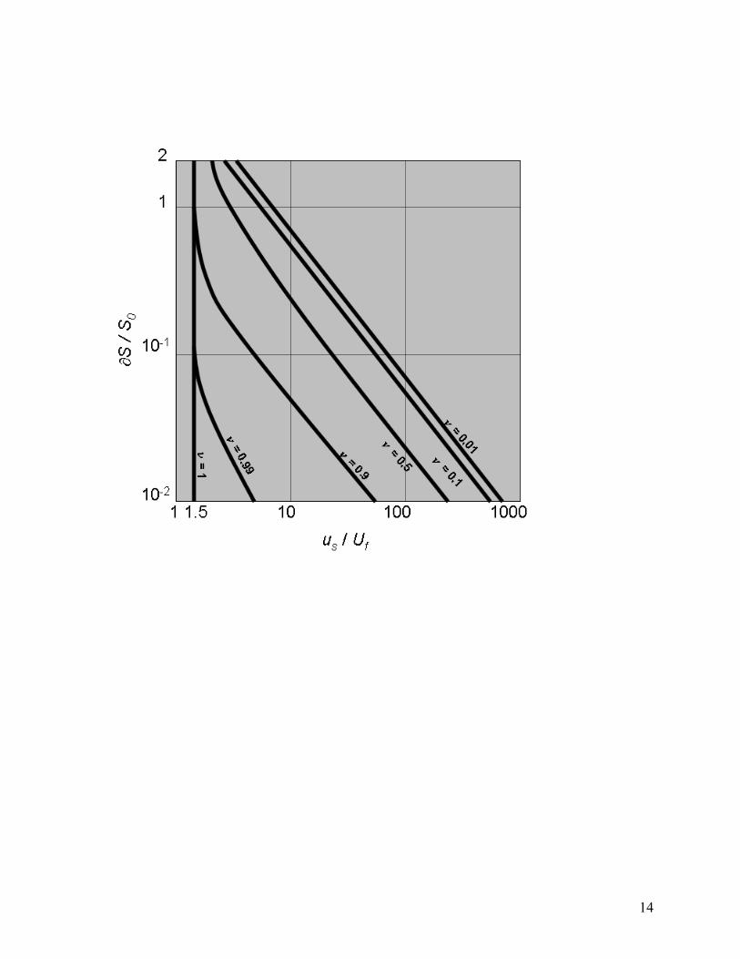
The two parameters described above can be used to characterize the nature of salt

transport in estuaries. The contribution by the diffusive portion (vs the advective portion) of the

total salt flux into the estuary can be called ν. The parameter ν may oscillate between 0 and 1.

When ν is close to 0, up-estuary salt transport is dominated by advection, i.e., by the

gravitational circulation. In this case, mixing processes are weak, as in a highly stratified estuary

5

(fjord). When ν approaches 1, the total salt transport is dominated by diffusive processes (e.g.

tidal mixing) as in unidirectional net flows. The parameter ν may be portrayed in terms of the

stratification and circulation parameters (Fig. 1.4). This diagram shows that salt transport is

dominated by advective processes under high gravitational circulation or strongly stratified

conditions. It also shows that diffusive processes dominate the salt flux at low circulation

parameter (unidirectional net flows) regardless of the stratification parameter. Between those

two extremes, the salt transport has contributions from both advective and diffusive processes.

The more robust the stratification and circulation parameters, the stronger the contribution from

advective processes to the total salt flux will be.

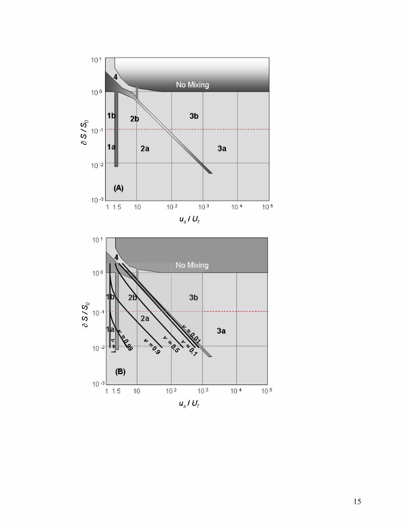
These concepts can be used to place estuaries in the parameter space of the circulation

and stratification parameters. The lower left corner of the parameter space (Fig. 1.5A) describes

well-mixed estuaries with unidirectional net outflows, i.e., seaward flows with no vertical

structure or type 1 estuaries. These are well-mixed estuaries, type 1a, implying strong tidal

forcing and weak river discharge (or large tidal prisms relative to freshwater volumes). There

are also estuaries with depth-independent seaward flow but with highly stratified conditions.

These type 1b estuaries have large river discharge compared to tidal forcing. In type 1 estuaries,

in general, the upstream transport of salt is overwhelmingly dominated by diffusive processes (ν

≈ 1, Fig. 1.5B).

Type 2 (Fig. 1.5B) estuaries are those where flow reverses at depth and include most

temperate estuaries. These systems feature well-developed gravitational circulation and exhibit

contributions from advective and diffusive processes to the upstream salt transport (0.1 < ν <

0.9). Type 2a estuaries are well-mixed or weakly stratified and type 2b estuaries are strongly

stratified. Note that strongly stratified and weakly stratified estuaries of type 2 may exhibit

similar features in terms of the relative contribution from diffusive processes to the upstream salt

transport (Fig. 1.5B).

Type 3 estuaries are associated with fjords, where gravitational circulation is well-

established: strong surface outflow and very small depth-averaged flows, typical of deep basins.

This flow pattern results in large values (>100-1000) of the circulation parameter (Fig. 1.5A).

Type 3a estuaries are moderately stratified and Type 3b are highly stratified. The peculiarity

about these systems is that the upstream transport of salt is carried out exclusively by advective

processes (ν <0.01, Fig. 5b).

6

Finally, type 4 estuaries exhibit seaward flows with weak vertical structure and highly

stratified conditions as in a salt-wedge estuary. In type 4 estuaries, the diffusive fraction ν lines

tend to converge, which indicates that in type 4 estuaries, salt transport is produced by both

advective and diffusive processes. In the Hansen-Rattray diagram, it is noteworthy that some

systems will occupy different positions in the parameter space as stratification and circulation

parameters change from spring to neap tides, from dry to wet seasons, and from year to year.

Analogous to the classification of estuaries in terms of the two non-dimensional

parameters discussed above, estuarine systems can also be classified in terms of the lateral

structure of their net exchange flows. The lateral structure may be strongly influenced by

bathymetric variations and may exhibit vertically sheared net exchange flows, i.e., net outflows

at the surface and near-bottom inflows (e.g. Pritchard, 1956), or laterally sheared exchange flows

with outflows over shallow parts of a cross-section and inflows in the channel (e.g. Wong, 1994).

The lateral structure of exchange flows may ultimately depend on the competition between

Earth’s rotation (Coriolis) and frictional effects (Kasai et al., 2000) as characterized by the

vertical Ekman number (Ek). But the lateral structure of exchange flows also may depend on the

Kelvin number (Ke), which is the ratio of the width of the estuary to the internal radius of

deformation.

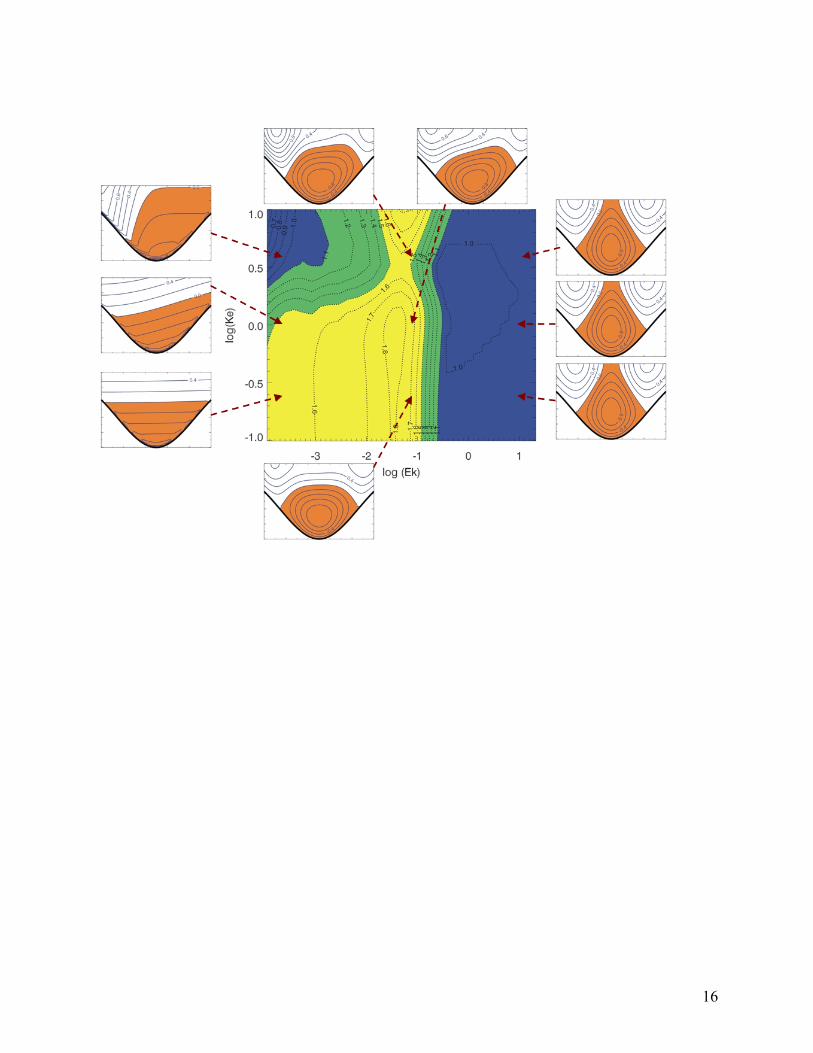
The Ekman number is a non-dimensional dynamical depth of the system. Low values of

Ek imply that frictional effects are restricted to a thin bottom boundary layer (weak frictional,

nearly geostrophic conditions) and high Ek values indicate that friction affects the entire water

column. The lateral structure of density-driven exchange flows may be described in terms of

whether the flows are vertically sheared or unidirectional in the deepest part of the cross-section

(Valle-Levinson et al., 2008). Under low Ek (< 0.001, i.e., < -3 in the abscissa of Fig. 1.6) the

lateral structure of exchange flows depends on the dynamic width of the system (Fig. 1.6). In

wide systems (Ke > 2, i.e., >0.3 in th eordinate of Fig. 1.6), outflows and inflows are separated

laterally according to the Earth’s rotation, i.e. the exchange flow is laterally sheared. In narrow

systems (Ke < 1, i.e. <0 in the ordinate of Fig.1.6) and low Ek (still < 0.001, i.e., <-3 in the

abscissa), exchange flows are vertically sheared. In contrast, under high Ek ( > 0.3, i.e., >-0.5 in

the abscissa of Fig. 1.6) and for all Ke the density-driven exchange is laterally sheared

independently of the width of the system. Finally, under intermediate Ek (0.01 < Ek < 0.1, i.e.,

7

between -2 and -1 in the abscissa), the exchange flow is preferentially vertically sheared but

exhibiting lateral variations.

The main message is that under weak friction (Ek < 0.01), both depth and width are

important to determine whether the density-driven exchange is vertically or horizontally sheared.

This is illustrated by the fact that the contour values in the entire region of Ek < 0.01 (i.e. <-2 in

the abscissa) in Figure 1.6 vary with both Ek and Ke. In contrast, under Ek > 0.01 the depth is

the main determinant as to whether the exchange is vertically or horizontally sheared. This is

shown by fact that the contour values in Figure 1.6 vary mostly with Ek but very little with Ke.

A future challenge of this approach is to determine the variability of a particular system in the Ek

vs Ke parameter space. It is likely that an estuary will describe an ellipse of variability in this

plane from spring to neaps and from wet to dry seasons or from year to year.

All of the above classifications depend on diagnostic parameters that require substantial

information about the estuary, i.e., on dependent variables. In addition, they do not take into

account the effects of advective accelerations, related to lateral circulation, that may be of the

same order of magnitude as frictional effects (e.g. Lerczak and Geyer, 2004). Some of these

nuances are discussed further in Chapter 5 of this text. Future schemes will require taking those

advective effects into account. In the following chapter, in addition to presenting the basic

hydrodynamics in estuaries, another approach for classifying estuaries based on different

dynamical properties is discussed. Such an approach, consistent with that of Prandle (2009),

uses only the river discharge velocity and the tidal current velocity as the parameters needed to

classify estuaries.

8

Figure 1.1. Types of estuaries on the basis of water balance. Low inflow estuaries exhibit a ‘salt

plug.’

Figure 1.2. Classification of estuaries on the basis of geomorphology.

Figure 1.3. Classification of estuaries on the basis of vertical structure of salinity.

Figure 1.4. Diffusive salt flux fraction in the stratification/circulation parameter space (re-drawn

from Hansen and Rattray, 1966).

Figure 1.5. Classification of estuaries according to hydrodynamics, in terms of the circulation

and stratification parameters (redrawn from Hansen and Rattray, 1966). (A) Type 1 estuaries

show no vertical structure in net flows; in type 2 estuaries, the net flows reverse with depth;

type 3 estuaries exhibit strong gravitational circulation; and type 4 estuaries are salt wedge.

(B) Includes lines of diffusive salt flux showing the dominance of advective salt flux for type

3 estuaries and diffusive flux for type 1.

Figure 1.6. Classification of estuarine exchange on the basis of Ek and Ke. The subpanels

appearing around the central figure denote cross-sections, looking into the estuary, of

exchange flows normalized by the maximum inflow. Inflow contours are negative and

shaded in orange. The vertical axis is non-dimensional depth from 0 to 1 and the horizontal

axis is non-dimensional width, also from 0 to 1. The central figure illustrates contours of the

difference between maximum outflow and maximum inflow over the deepest part of the

channel and for different values of Ek and Ke. Note that the abscissa and ordinate represent

the logarithm of Ek and Ke. Blue-shaded contour regions denote net inflow throughout the

channel, i.e., laterally sheared exchange flow as portrayed by the subpanels whose arrows

point to the corresponding Ek and Ke in the blue regions. Yellow-shaded contour regions

illustrate vertically sheared exchange in the channel as portrayed by the subpanels whose

arrows point to the corresponding Ek and Ke in the yellow regions. Green regions represent

vertically and horizontally sheared exchange flow, similar to the second subpanel on the left,

for log (Ke) equal 0 and log (Ek) ~ -3.7.

9

References

Cameron, W. M. and D. W. Pritchard (1963) Estuaries. In M. N. Hill (editor): The Sea vol. 2,

John Wiley and Sons, New York, 306 - 324.

Hansen, D. V. and M. Rattray jr. (1966) New dimensions in estuary classification. Limnology

and Oceanography 11, 319 - 326.

Kasai, A., A. E. Hill, T. Fujiwara, and J. H. Simpson (2000), Effect of the Earth’s rotation on the

circulation in regions of freshwater influence, J. Geophys. Res. 105(C7), 16,961– 16,969.

Lerczak, J.A., and W. Rockwell Geyer, 2004: Modeling the lateral circulation in straight,

stratified estuaries, J. Phys. Oceanogr., 34, 1410–1428.

Prandle (2008) missing

Pritchard, D. W. (1952) Estuarine hydrography. Advances in Geophysics 1, 243 - 280.

Pritchard, D. W. (1955) Estuarine circulation patterns. Proceedings of the American Society of

Civil Engineers 81 (717), 1 - 11.

Pritchard, D.W. (1956) The dynamic structure of a coastal plain estuary. J. Marine. Res. 15, 33-

42.

Valle-Levinson, A. (2008), Density-driven exchange flow in terms of the Kelvin and Ekman

numbers, J. Geophys. Res., 113, C04001, doi:10.1029/2007JC004144.

Wolanski, E. (1986) An evaporation-driven salinity maximum zone in Australian tropical

estuaries. Estuarine, Coastal and Shelf Science 22, 415-424.

Wong, K.-C. (1994) On the nature of transverse variability in a coastal plain estuary, J. Geophys.

Res. 99(C7), 14,209-14,222.

10

11

12

13

14

15

16