Effects of Resolution of Lighting

Control Systems

A thesis submitted in fulfilment of the requirements for

the degree of Doctor of Philosophy

Wenye Hu

Sydney School of Architecture, Design and Planning

The University of Sydney

2018

Supervisor:

Associate Professor Wendy Davis

Declaration

I, Wenye Hu, hereby certify that this thesis is my original work, except as acknowledged in

the text. I have not submitted this thesis, either in full or in part, for a degree at any other

university or institution. The experiments conducted for this thesis were done so under the

approval of the Human Research Ethics Committee of The University of Sydney.

Wenye Hu

1

Abstract

Advances in lighting technologies have spurred sophisticated lighting control systems

(LCSs). To conserve energy and improve occupants’ wellbeing, LCSs have been integrated

into sustainable buildings. However, the complexity of LCSs may lead to negative

experiences and reduce the frequency of their use. One fundamental issue, which has not

been systematically investigated, is the impact of control resolution (the smallest change

produced by an LCS). In an ideal LCS, the resolution would be sufficiently fine for users to

specify their desired lighting conditions, but the smallest change would be detectable. Thus,

the design of optimal control systems requires a thorough understanding of the detectability

and acceptability of differences in illuminance, luminance and colour. The control of colour

is complicated by the range of interfaces that can be used to facilitate colour mixing.

Four psychophysical experiments investigated the effect of LCS resolution. The first two

experiments explored the effect of resolution in white light LCSs on usability and energy

conservation. The results suggest that, in different applications, LCSs with resolutions

between 14.8 % and 17.7 % (of illuminance) or 26.0 % and 32.5 % (of luminance) have the

highest usability.

The third experiment evaluated the usability of three colour channel control interfaces based

on red, green, blue (RGB), hue, saturation, brightness (HSB) and opponent colour mixing

systems. Although commonly used, the RGB interface was found to have the lowest

usability.

2

The fourth experiment explored the effect of hue resolution, saturation resolution and

luminance resolution on the usability. Generally, middle range resolutions, which are

approximately between three and five times the magnitude of the just noticeable difference

(JND), for both hue and saturation were found to yield the greatest usability. The interaction

between these three variables was characterised.

Findings from this research provide a deeper understanding of the fundamental attribute of

control resolution and can guide the development of useful and efficient lighting control

systems.

3

Acknowledgements

I would like to thank my supervisor, Associate Professor Wendy Davis for her

encouragement and advice. It would never have been possible to write this thesis without her

incredible support.

I would also like to express my thanks to my associate supervisor Associate Professor Martin

Tomitsch for his valuable advice.

I also express a deep sense of gratitude to Sydney School of Architecture, Design and

Planning, which has opened the door to a new world for me.

Thanks also to my colleagues in the Lighting Lab: Bettina Easton, Dorukalp Durmus, Joelene

Elliott, Mariana Papa, Murray Robson and Simm Steel. It gives me immense pleasure to

work with them.

Finally, this thesis is dedicated to my late father, Tingmin Hu, whom I have been missing.

4

Publications Parts of this thesis have been published:

Chapter 3:

Hu, W., & Davis, W. (2016). Dimming curve based on the detectability and acceptability of

illuminance differences. Optics Express, 24(10), A885-A897.

https://www.osapublishing.org/oe/abstract.cfm?uri=oe-24-10-A885

Chapter 4:

Hu, W., & Davis, W. (2016). Luminance resolution of lighting control systems: usability and

energy conservation. Paper presented at CIE 2016 “Lighting Quality and Energy

Efficiency,” Melbourne, Australia.

Chapter 5:

Hu, W., & Davis, W. (2017). Development and evaluation of colour control interfaces for

LED lighting. Optics Express, 25(8), A346-A360.

https://www.osapublishing.org/oe/abstract.cfm?uri=oe-25-8-A346

Chapter 6:

Hu, W., & Davis, W. (in press). The effect of control resolution on the usability of colour-

tunable LED lighting systems. LEUKOS (2018)

5

Authorship attribution statement

As the co-author of the papers included in this thesis, I confirm that Wenye Hu’s contribution

to these papers is consistent with her being named as first author. Wenye was responsible for

the design and implementation of the experiments, the collection and analysis of the research

data, and the process of drafting the manuscripts.

As the co-author and Wenye’s supervisor, I provided general supervision of this research. My

contributions included primary development of the research concept and experimental design,

as well as the review and editing of the manuscripts.

Wendy Davis

6

Table of contents DECLARATION 1

ABSTRACT 2

ACKNOWLEDGEMENTS 4

PUBLICATIONS 5

AUTHORSHIP ATTRIBUTION STATEMENT 6

CHAPTER 1. INTRODUCTION 12

CHAPTER 2. LITERATURE REVIEW 19

2.1. Psychophysical measurements of visual perception 19

2.2. Control of light intensity to reduce energy consumption 25

2.3. Increasing use of colour-tunable LEDs 29

2.4. Preferences for colour 31

2.5. Colour vision and colour spaces 33

2.6. Colour differences 38

2.7. Lighting control interfaces 40

2.8. Usability assessment 45

CHAPTER 3. DIMMING CURVE BASED ON THE DETECTABILITY AND

ACCEPTABILITY OF ILLUMINANCE DIFFERENCES 57

3.1. Introduction 59

3.2. Previous studies 59

3.3. Methods 61

3.4. Results 65

3.5. Discussion 69

3.6. Conclusions 70

7

CHAPTER 4. LUMINANCE RESOLUTION OF LIGHTING CONTROL SYSTEMS:

USABILITY AND ENERGY CONSERVATION 71

4.1. Background 72

4.2. Methods 72

4.3. Results and discussion 74

4.4. Conclusions 82

CHAPTER 5. DEVELOPMENT AND EVALUATION OF COLOUR CONTROL

INTERFACES FOR LED LIGHTING 83

5.1. Introduction 85

5.2. Previous studies 85

5.3. Methods 86

5.4. Results 92

5.5. Discussion 95

5.6. Conclusions 96

5.7. Appendix 96

CHAPTER 6. THE EFFECT OF CONTROL RESOLUTION ON THE USABILITY OF

COLOUR-TUNABLE LED LIGHTING SYSTEMS 99

6.1. Introduction 100

6.2. Methods 102

6.3. Results 109

6.4. Discussion 118

6.5. Conclusions 121

CHAPTER 7. CONCLUSIONS 127

APPENDIX

Corrections to published articles 131

Lists of abbreviations 132

Ethics Approval 134

8

List of figures

Chapter 2:

Figure 1. Weber fraction as a function of background luminance for five different stimulus

sizes (Norton, Corliss & Bailey, 2002) 24

Figure 2. Relative luminous efficacy as a function of current (expressed as a percentage,

relative to the maximum) for a high-power white LED (Denicholas, 2017) 26

Figure 3. Colour matching functions �̅�(𝜆), �̅�(𝜆), 𝑏)(𝜆) 35

Figure 4. MacAdam ellipses magnified ten times (Schanda, 2007) 36

Figure 5. The circle of hues in the Swedish natural colour system (NCS) (Hunt & Pointer,

2011) 37

Figure 6. A typical control interface design based on a colour wheel, modified from the HSB

system 43

Figure 7. A typical control interface combining sliders with a colour wheel based on the HSB

system 44

Chapter 3:

Fig. 1. Experimental setup 61

Fig. 2. Plan view of the experimental setup 62

Fig. 3. Just noticeable difference (JND) in illuminance as a function of reference illuminance

65

Fig. 4. Matching errors and users’ confidence in matching accuracy as a function of LCS

resolution 66

Fig. 5. The effect of control resolution on the normalized number of button presses 66

Fig. 6. Mean normalized speed per button press and subjective ratings 67

Fig. 7. The proposed step-dimming curve with a resolution of 17%, compared to a continuous

logarithmic dimming curve 68

Fig. 8. The proposed step-dimming curve with a resolution of 7%, compared to a continuous

logarithmic dimming curve 68

9

Fig. 9. The proposed step-dimming curve with a resolution of 17%, compared to a continuous

Square Law dimming curve 69

Chapter 4:

Figure 1 – (a) Experimental setup (b) Section view of the experimental setup 73

Figure 2 – Just noticeable difference (JND) as a function of reference luminance for the

2AFC experiment 75

Figure 3–Detection thresholds for luminance differences for five subjects 75

Figure 4 – The probability distribution of the matching errors (percentage of reference

luminance) across all participants 76

Figure 5 – Matching error as a function of control resolution 77

Figure 6 – Normalized matching time as a function of resolution 77

Figure 7 – Normalized number of button presses as a function of resolution 78

Figure 8 – Normalized speed per button press as a function of resolution 79

Figure 9 – Frequency distributions of questionnaire responses 80

Figure 10 – The proposed step-dimming curve (red line) compared to a traditional continuous

logarithmic dimming curve (blue line), with a resolution of 32.5 % 81

Figure 11 – The proposed step-dimming curve (red line) compared to a Square Law dimming

curve (blue line), with a resolution of 32.5 % 81

Figure 12 – The proposed step-dimming curve (red line) compared to a traditional continuous

logarithmic dimming curve (blue line), with a resolution of 13 %. 82

Chapter 5:

Fig. 1. Experimental setup 86

Fig. 2. Plan view of the experimental setup 87

Fig. 3. Relative power as a function of wavelength for the light used in the test booth 87

Fig. 4. Luminance as a function of the DMX values for each primary light 88

Fig. 5. The button box used in the experiment 89

Fig. 6. Six reference colours and colour gamut plotted on CIE 1976 (u’, v’) chromaticity

diagram 91

Fig. 7. Chromaticity matching error (Δ u’v’) using different colour control interfaces 93

Fig. 8. Luminance matching error (ΔL) for different colour control interfaces 93

10

Fig. 9. Completion time (in seconds) of the matching task using different interfaces 94

Fig. 10. Label on the button box for RGB control 97

Fig. 11. Colour settings for HSB interface 97

Fig. 12. Label on the button box for HSB control 97

Fig. 13. Label on the button box for opponent colour control 98

Chapter 6:

Fig. 1 The reflectance of the white panels used for the booths 103

Fig. 2 Experimental setup 103

Fig. 3 Experimental setup (from the observer’s back) 104

Fig. 4 The colour control interface on the button box 105

Fig. 5 Luminance as a function of DMX value for each colour channel and each luminaire105

Fig. 6 Relative power as a function of wavelength for the luminaires used in the target booth

(a) and test booth (b) 106

Fig. 7 (a) When the “Saturation +” button was pressed, the CIELAB coordinates of the test

colour changed from point “colour 0” to point “colour 1,” with a saturation increment of the

given saturation resolution, while the luminance and hue angle of the colour remained

constant. 108

Fig. 7 (b) When the “Hue +” button was pressed, the CIELAB coordinates of the colour

changed from point “colour 0” to point “colour 1,” with a hue change of the given hue

resolution, while the luminance and chroma of the test colour remained constant 108

Fig. 8 The effect of hue resolution on the effectiveness and efficiency of colour-tunable

LCSs 113

Fig. 9 The effect of saturation resolution on the effectiveness and efficiency of colour-tunable

LCSs 114

Fig. 10 Interaction between hue and saturation resolutions on completion times 117

11

Chapter 1. Introduction

Over the past decade, light-emitting diodes (LEDs) have made significant contributions to the

reduction of energy consumption for lighting, without causing mercury pollution (National

Academies of Sciences, Engineering and Medicine, 2017). However, LEDs do not reach their

full potential until they are connected to advanced lighting control systems (LCSs). Newer

lighting technologies integrated into sophisticated lighting control systems offer tremendous

opportunities to improve lighting environments in architectural spaces. There is no doubt that

the thoughtful use of LCSs can considerably reduce the energy consumed by lighting (Boyce

et al., 2006; Gentile, Laike, & Dubois, 2016; Jennings, Rubinstein, DiBartolomeo, & Blanc,

2000; Lowry, 2016; Roisin, Bodart, Deneyer, & D’Herdt, 2008). The use of LCSs is

incentivized by many sustainable building rating systems, such as Leadership in Energy and

Environmental Design (LEED) (DiLouie, 2009).

Energy conservation is not the only motivation for using LCSs in modern buildings. One

experiment, in which there were 118 participants, suggested that, in offices where LCSs were

used, occupants experienced significant improvements in mood, satisfaction with the lighting,

self-assessed productivity, subjective appraisal of the space, satisfaction with performance,

and several related measures (Newsham, Veitch, Arsenault, & Duval, 2004). Researchers

further found that those improvements were not actually caused by the lighting control

product itself, but by the freedom provided by an LCS for occupants to specify their desired

lighting conditions. Participants who made the largest adjustments to the lighting conditions

tended to report the greatest improvements in outcomes, while those who made small

changes reported insignificant improvements (Newsham et al., 2004).

Boyce and his colleagues also found that users preferred to have lighting control systems,

although their experiment did not demonstrate a correlation between the use of LCSs and

users’ positive moods. The results showed that participants used the lighting control system

to adjust the illuminance when engaging in different tasks, but the way they used the control

system varied widely. Some participants adjusted the illuminance slightly; some changed it

over the entire available range (Boyce, Eklund, & Simpson, 2000). The diversity of user

behaviour and preferences for illuminance may suggest a need for the ability to customise

lighting environments through LCSs.

12

Control systems can be classified into three types: manual, semi-manual, and automatic. The

difference between manual and automatic control is the extent to which a human body is

physically involved. Semi-manual typically refers to manual control systems with some pre-

set functions or scenes (Escuyer & Fontoynont, 2001). In a field study involving 41 office

workers, the acceptability of these three types of LCSs was evaluated. Automatic dimming in

the buildings was found “not annoying” for the occupants, while manual dimming was “more

likely to produce conscious satisfaction.” The results led the researchers to suggest that an

ideal LCS should allow users to select and adjust illumination manually rather than just

provide automatic control or semi-manual control (Escuyer & Fontoynont, 2001).

Recently, many manufacturers have released “smart” lighting systems or “intelligent”

lighting systems (Philips, 2018a; Schneider, 2017). In those systems, lamps/luminaires are

connected to the internet, sensors, or other appliances and lighting conditions can be changed

automatically in response to the information provided to the lighting system. Those systems

usually provide users with manual control as well, via small remote controllers, touch

screens, or smartphone displays (LIFX, 2017; Philips, 2018). Hence, control interfaces for

LCSs have been undergoing radical change. Conventional light switches, such as toggle

switches, slide dimmers and knob dimmers, have been re-designed, improved, or fully

replaced by modern tangible user interfaces, which are designed to control digital signals

through tangible objects. Not only are more control interface options provided to users, but

the dimensions of control are also increasing. Conventional light dimming systems have only

one control dimension, in which users increase or decrease the luminous output of the

luminaires. Because of the nature of LEDs, a modern lighting system today is capable of

providing users with control over a range of dimensions, such as the colour properties (e.g.

hue and saturation), brightness (e.g. luminance, illuminance) or even light distribution (i.e.

the pattern of light throughout the space). Users may use relatively small control interfaces,

to adjust complex lighting parameters. However, general end-users of LCSs, who are not

well-trained lighting experts, may find the complex LCSs “too cumbersome to use” and not

acceptable (Lucero, Lashina, & Terken, 2006).

With the proliferation of digital technologies, a large range of user interfaces for LCSs have

been designed to engage users and improve their satisfaction and productivity. Interface

designers are already aware of the vast opportunities brought by the revolution of LCSs, as

well as the need to deeply understand user interactions with LCSs. While the lighting

13

industry focuses primarily on the interface between the LCSs and the luminaires, some

researchers in human computer interaction (HCI) have assessed the usability of interactive

systems. Their research is discussed in Section 2.8. However, the fundamental principles

underlying the design of LCSs are not well understood, such as the mathematical conversion

from users’ control inputs to device-specific control signals, visual discrimination thresholds,

psychologically acceptable magnitudes of change generated by an LCS, etc. Mathematical

conversions between user inputs and device control signals have been actively studied in the

television and computer display industry, but their results might not be directly applicable to

the lighting industry.

Control resolution, which underlies all LCSs, is one of the parameters that have been

overlooked in lighting industry. The term “resolution” is defined to be “the smallest interval

measurable by a telescope or other scientific instrument”, according to Oxford dictionary

(“Resolution,” 2016). In this project, the term “resolution” will be used in this way to refer to

the smallest change that can be produced by a lighting control system. In a conventional

analogue dimming system, the luminous flux of a luminaire could not be specified precisely

by a user, so the resolution of the LCSs could not be easily defined. However, advanced

digital LCSs can offer high resolutions. Theoretically, an 8-bit LCS can adjust the luminous

flux of a light source in 256 levels. A colour-tunable LED system with three primary colours

can generate more than 16 million colours. Such commercial products have already been

used in architectural spaces (Halper, 2017). Some colour-tunable LED systems recently

introduced have up to eight 16-bit channels, which provide 3 × 1038 colour options, though

they would not all be able to visually distinguished (Telelumen, 2016). Although high

resolutions allow end-users to select their desired options more accurately, the extremely high

resolutions may also lead to users’ confusion, loss of productivity, and frustration. It seems

commonly accepted that low-resolution LCSs would lead to dissatisfaction, since users

would not always be able to choose their desired luminous output (in white light systems) or

desired colours (in colour-tunable systems). But the effect of resolution on the usability of

LCSs is not well understood. Little empirical data is available to test the hypothesis that high

resolutions lead to high usability or are beneficial for the end-users.

Negative experiences using LCSs might reduce the frequency with which a user interacts

with the system. Researchers have found that negative consumer experiences with energy-

efficient products significantly slow widespread adoption (Sandahl, Gilbride, Calwell, &

14

Ledbetter, 2006). Negative user experiences may also discourage occupants from using the

systems in the ways they are designed to be used. Since many control systems aim to

conserve energy, a lack of use or/and inappropriate usage could result in the wasted electrical

energy, as well as unnecessary hardware costs associated with installing the LCSs.

In this project, it is hypothesised that extremely high LCS resolution does not ensure an

efficient and effective system or increased user satisfaction. To develop a systematic

understanding of the effects of LCS resolution, four psychophysical experiments were

conducted. When the resolution is so extremely high that the magnitude of the change

generated by an LCS is smaller than one just noticeable difference (JND), the changes cannot

be perceived at all. The resolution settings described in this research were based on the just

noticeable difference (JND) in visual perception, which is discussed in Section 2.1. Colour

vision and colour differences are discussed in Sections 2.5 and 2.6. In this research, the

optimal ranges of resolutions were explored to help the design of future LCSs.

The four experiments presented in this thesis employed quantitative research methods to

measure objective and subjective dependent variables. For the objective variables,

psychophysical methods were used, while for subjective variables, questionnaires were used

to assess users’ satisfaction. The usability of LCSs with various resolutions was assessed by

the participants’ performance in matching tasks, as well as their satisfaction, expressed by

subjective ratings in questionnaires. The literature underlying the methods used to evaluate

usability is discussed in Section 2.8.

The first experiment in this research investigated the detectability and acceptability of

illuminance differences of white light. A two-alternative-forced-choice (2AFC) method was

used to examine the just noticeable difference in illuminance. The method of adjustment,

another classic psychophysical method, was used to investigate users’ acceptance of

illuminance differences when using an LCS. An optimal range of resolutions was suggested

to yield good usability for dimming systems. Based on the results of detectable and

acceptable illuminance difference, a series of step-dimming curves, which generate

undetectable or acceptable reductions in illuminance, were proposed to save energy in

different applications. Energy can also be reduced by diminishing negative user experiences

with LCSs. The first experiment and its implications for energy consumption are discussed in

Chapter 3.

15

When people use an LCS, they may look at the illuminated surfaces, such as the walls of a

room, or at the luminaires directly. This may depend on the interface design of the control

systems, the luminance of luminaires or simply the users’ habits. To understand the effects of

resolution deeply, both illuminance and luminance resolution were explored. The second

experiment was conducted using an approach similar to the first experiment to investigate the

effect of luminance resolution on usability. This is discussed in Chapter 4.

The proposed series of step-dimming curves in Chapters 3 and 4 might further conserve

energy by counteracting LED efficacy droop, which is discussed in Section 2.2. Luminous

efficacy decreases as LED luminous flux increases. If an LCS reduces the luminous output of

a light source by an unperceivable or acceptable magnitude, the lighting system would

operate more efficaciously.

Section 2.3 discusses the increasing use of colour-tunable lighting systems. The use of

colour-tunable lighting systems for architectural applications has emerged in recent years.

Since users’ colour preferences are difficult to predict, as discussed in Section 2.4, LCSs can

allow users to select their desired colours. Many commercially available colour-tunable LCS

interfaces use two or three control dimensions to specify the colour of light. One common

method uses each dimension to control the intensity of each primary colour (red, green, blue)

to mix the coloured light, commonly referred to as RGB colour mixing. However, there are

conflicting results about the usability of RGB interfaces in the literature on computer

displays, which is discussed in Section 2.7. In the third experiment, it was hypothesised that

RGB LCS interfaces might not yield high usability. Comparisons of effectiveness, efficiency

and user satisfaction were made among LCSs based on an RGB interface, HSB interface

(hue, saturation and brightness) and opponent colour interface. This is discussed in Chapter 5.

Results from the third experiment suggested that the HSB interface yielded higher usability

than the RGB interface. Thus, the fourth experiment studied the effect of resolution based on

the HSB interface. Four resolutions of the three control dimensions (hue, saturation and

brightness dimensions) were examined. The effect of each single control dimension, as well

as the interaction between two or more dimensions, is discussed in Chapter 6. Chapter 7

integrates the findings across this research project and provides suggestions for future studies.

16

References

Boyce, P. R., Eklund, N. H., & Simpson, S. N. (2000). Individual Lighting Control: Task

Performance, Mood, and Illuminance. Journal of the Illuminating Engineering

Society, 29(1), 131-142. doi:10.1080/00994480.2000.10748488

Boyce, P. R., Veitch, J. A., Newsham, G. R., Jones, C. C., Heerwagen, J., Myer, M., &

Hunter, C. M. (2006). Occupant use of switching and dimming controls in offices.

Lighting Research & Technology, 38(4), 358-376. doi:10.1177/1477153506070994

DiLouie, C. (2009). The LEED View: Sustainable Lighting. Retrieved from

http://www.ecmag.com/section/lighting/leed-view-sustainable-lighting

Escuyer, S., & Fontoynont, M. (2001). Lighting controls-- a field study of office workers’

reactions. Lighting Research & Technology,33(2).

Gentile, N., Laike, T., & Dubois, M.-C. (2016). Lighting control systems in individual offices

rooms at high latitude: Measurements of electricity savings and occupants’

satisfaction. Solar Energy, 127(Supplement C), 113-123.

doi:https://doi.org/10.1016/j.solener.2015.12.053

Halper, M. (2017). Philips turns modern Hanoi bridge into a colorful light display. Retrieved

from http://www.ledsmagazine.com/articles/2017/07/philips-turns-modern-hanoi-

bridge-into-a-colorful-light-display.html

Jennings, J. D., Rubinstein, F. M., DiBartolomeo, D., & Blanc, S. L. (2000). Comparison of

control options in private offices in an advanced lighting controls testbed. Journal of

the Illuminating Engineering Society, 29(2), 39-60.

LIFX. (2017). LIFX Wi-Fi LED Lights. Retrieved from

https://www.lifx.com.au/collections/featured-products

Lowry, G. (2016). Energy saving claims for lighting controls in commercial buildings.

Energy and Buildings, 133(Supplement C), 489-497.

doi:https://doi.org/10.1016/j.enbuild.2016.10.003

Lucero, A., Lashina, T., & Terken, J. (2006). Reducing complexity of interaction with

advanced bathroom lighting at home (Reduktion der Interaktionskomplexität bei

hochentwickelten Badezimmerbeleuchtungssystemen für die Heimanwendung). i-

com, 5(1/2006), 34-40.

National Academies of Sciences, Engineering and Medicine. (2017). Assessment of Solid-

State Lighting, Phase Two. Washington, DC: The National Academies Press.

17

Newsham, G., Veitch, J., Arsenault, C., & Duval, C. (2004). Effect of dimming control on

office worker satisfaction and performance. Paper presented at the Proceedings of the

IESNA annual conference.

Philips. (2018a). Your personal Wireless lighting system. Retrieved from

https://www2.meethue.com/en-au/about-hue

Resolution. (2016). In Oxford English Dictionary: Oxford University Press. Retrieved from

https://en.oxforddictionaries.com/definition/resolution

Roisin, B., Bodart, M., Deneyer, A., & D’Herdt, P. (2008). Lighting energy savings in offices

using different control systems and their real consumption. Energy and Buildings,

40(4), 514-523. doi:10.1016/j.enbuild.2007.04.006

Sandahl, L., Gilbride, H. S. T., Calwell, C., & Ledbetter, M. (2006). Compact Fluorescent

Lighting in America- Lessons Learned on the Way to Market. the U.S. Department of

Energy.

Schneider Electric. (2017). Lighting control. Retrieved from https://www.schneider-

electric.com.au/en/product-range-download/6901-lighting-control#tabs-top

Telelumen. (2016). Products. Retrieved from http://www.telelumen.com/products2.html

18

Chapter 2. Literature review

2.1. Psychophysical measurements of visual perception

Visual experience is subjective and can be difficult to communicate precisely. Verbal

descriptions of visual experiences offer some information but may not be strictly reliable in

scientific research. People experiencing the same perception may not express their experience

similarly. Hofstetter et al. (2000, as cited in Norton, Corliss, & Bailey, 2002) defined

perception as an “appreciation of a physical situation through the mediation of one or more

senses”. It is generated inside the brain and is unable to be measured directly. However,

external stimuli, to some extent, reflect the internal sensation and perception evoked (Norton

et al., 2002). Thus, in vision science, researchers have developed methods to relate perceptual

magnitude to the physical parameters of stimuli, which are measurable. Introduced by

Fechner and improved by numerous pioneers in sensory research, psychophysical methods

are commonly used in visual perception research. Psychophysics seems to be a paradox, since

“it requires the objectification of subjective experience” (Windhorst & Johansson, 2012).

Although experimental methods may vary for different objectives, the fundamental principle

of psychophysics is to use the physical parameters as a reference for assessing perceptual

experience (Wade & Swanston, 2013; Windhorst & Johansson, 2012). For instance,

measurements of observers’ performance in a visual task may characterise the observers’

perception of the visual environment.

Many psychophysical studies have examined the limits or thresholds of perception, such as

detection thresholds and discrimination thresholds (Pelli & Farell, 1995). The term

“threshold” refers to the boundary between a stimulus magnitude that causes one response

and the stimulus magnitude that causes a different response (or non-response) (Norton et al.,

2002). Detection thresholds, also known as absolute thresholds, refer to the smallest

magnitude at which the presentation of a stimulus can be just detected. Discrimination

thresholds are the difference in magnitude between two stimuli when they can barely be

distinguished. A discrimination threshold is sometimes referred to as a difference threshold or

a just noticeable difference (JND) (Wade & Swanston, 2013). It is not necessary or beneficial

for a lighting control system to have an extremely fine resolution, in which a change

generated by a users’ input cannot be detected. Although modern digital control systems offer

19

extremely fine resolutions, the smallest change generated by the system should be greater

than a JND.

Psychophysics comprises various methods for different types of tasks undertaken by

observers. A simple and quick method is the method of adjustment, in which experimenters

instruct observers to achieve a certain perceptual criterion and observers directly adjust the

physical parameter of the stimulus to meet the criterion (Pelli & Farell, 1995). Due to the

subjective nature of adjustments, the instructions given to the participants are vital. A

straightforward and easy to understand instruction is to match two stimuli (Farell & Pelli,

1999). Matching experiments are commonly used, in which two stimuli are presented and

observers are instructed to match one (usually referred to as the test stimulus) to the other

(the reference or target stimulus). For example, in a luminance matching experiment,

observers adjust the luminance of a test stimulus to match the reference stimulus. This

method relies on observers’ control of stimuli and is based on what they perceive or what

they believe they perceive (Windhorst & Johansson, 2012).

The two-alternative-forced-choice (2AFC) method, which was first introduced by Bergmann

in 1858, is considered to be more objective than the method of adjustment (Windhorst &

Johansson, 2012). In a typical 2AFC experiment, two, and only two, stimuli are provided to

the observers, who have to choose one according to the instructed criterion. For instance,

observers may be shown two stimuli marginally different in luminance and they must choose

the one that is brighter. The experimental data can be expressed as a psychometric function,

which is the proportion of correct judgments as a function of the luminance difference. A

percentage of correct judgments of approximately 50 %, which is a chance level of

performance, suggests that observers are unable to detect the luminance difference. A

percentage of correct responses of 75 %, which is above the chance level, is usually

considered to be the discrimination threshold. In this case, the just noticeable difference in

luminance can be read off the psychometric function at the level of 75 % correct judgments.

Psychophysicists have found that some differences, which observers claim cannot be detected

in other experiments, can in fact be detected correctly in 2AFC experiments (Windhorst &

Johansson, 2012). Thus, 2AFC is more sensitive than the method of adjustment in studies of

discrimination threshold.

20

There is not an abrupt change-point between detectable and undetectable differences in

stimulus magnitude. When a stimulus changes in magnitude, it gradually transitions between

being detectable and non-detectable. Discrimination threshold (difference threshold, JND) is

simply a statistical concept (Pelli & Farell, 1995; Wade & Swanston, 2013).

Determining the range of resolutions to be examined was an essential step for the research

presented in this thesis. Theoretically, the smallest change generated by a lighting control

system should be a detectable difference. Thus, visual perception literature was reviewed to

understand discrimination thresholds.

The terms “brightness discrimination” and “intensity discrimination” were widely used in

early published papers on the study of visual function. Brightness is a perceptual attribute

“reflecting the neural response to the intensity of a stimulus light” (Norton et al., 2002). It is

affected by the intensity of the stimulus, as well as the environment and state of the observer,

whereas luminance is a photometric measure, which is converted from radiance considering

the human luminous efficiency function (DeCusatis, 1997; Wyszecki & Stiles, 1982). Many

researchers interested in brightness or intensity discrimination, actually examined luminance

discrimination, which is a more technically accurate term for lighting. In this section,

“luminance discrimination” or “illuminance discrimination” will be used when the

researchers clearly stated the quantities they studied. Otherwise, intensity or brightness will

be generally used to include both/either.

Earlier visual perception research found that JND increases as the stimulus intensity

increases. Weber’s Law, named after Ernst Heinrich Weber (1795–1878), states that the

discrimination threshold (JND) is constantly proportional to the original stimulus magnitude.

Differences in luminance that are perceptibly different can be mathematically expressed by:

∆++= 𝑘 (1)

where ΔL is the threshold luminance difference, L is the background (or reference)

luminance, and k is a constant called the Weber fraction (Norton et al., 2002).

21

Although some publications refer to Weber’s Law as Weber-Fechner’s Law, it is a

misconception that Weber’s Law equates to Fechner’s Law. In fact, Weber’s Law posited a

linear relationship between discrimination threshold (ΔL) and background or reference

stimulus (L). Fechner, who was Weber’s student, expanded Weber’s Law to quantify

subjective sensory magnitude of a stimulus. He described a logarithmic relation between

sensory magnitude and stimulus magnitude, which is known as Fechner’s Law:

𝜓 = 𝑘log(𝛷) (2)

Where 𝜓is the sensory magnitude, k is a constant and 𝛷 is the stimulus magnitude (Fechner,

1851; Norton et al., 2002).

The relationship characterized by Weber’s Law is entirely between physical parameters,

while Fechner’s Law relates the psychological parameter with the physical parameter.

Fechner’s idea was to precisely scale the intensity of sensations, such as light brightness or

sound loudness, to their physical dimensions. He attempted to develop a systematic way to

express sensory magnitude as a quantitative index. He defined a system in which all sensory

intensities could be described with a common unit. The unit he selected was the JND (Wade

& Swanston, 2013).

Although Fechner’s Law appears in almost every textbook on psychophysics, critics argue

and debate this law. In the paper titled “To honor Fechner and repeal his law,” Stevens

claimed “a power function, not a log function describes the operating characteristics of a

sensory system.” He established a new law, which is usually referred to as Steven's Power

Law, showing a power relation between the magnitude of a physical stimulus and its

perceived intensity (Stevens, 1961). Steven’s Power Law can be expressed as:

𝑆 ∝ 𝐼7 (3)

where S is the magnitude of sensation and I is the stimulus intensity. The value of exponent n

varies according to the attributes of the stimulus.

22

One remarkable achievement of Steven’s research is the establishment of the value of the

exponent for a wide range of sensations including vision, audition, and odour recognition.

For instance, n equals 0.6 for loudness and 0.5 for brightness (Wade & Swanston, 2013).

Steven’s Power Law also reveals some fundamental aspects of colour measurement, such as

the relationship between CIE XYZ tristimulus values and the chroma and lightness in CIE

1976 (L*, a*, b*) colour space (Fairchild, 2013).

As part of the debate surrounding Fechner’s (logarithmic) Law and Steven’s Power Law,

Krueger proposed a creative method for reconciling them. When the exponent is less than

1.0, the plot of Stevens’ Power Law is not significantly different than the plot of Fechner’s

Law (Norton et al., 2002). Krueger suggested the use of a mathematic model to develop a

unified law. He showed that with different constants k and e, the power law and logarithmic

law can be very similar. When the exponent equals 0.1, 0.02 or 0.001, the logarithmic

function is indistinguishable from the power function (Krueger, 1989).

Since all of these laws were created by fitting data, Krueger’s suggestion might be

reasonable. Differences between Fechner’s and Steven’s laws are quantitative, rather than

qualitative. Although debate continues, Weber’s Law is better accepted than the other laws. If

the magnitude of observer perception is not needed, Weber’s Law is suitable. Otherwise, a

power law or logarithmic law is appropriate (Wade & Swanston, 2013).

The linear relationship makes Weber’s law appear to be straightforward. However, it is

complicated by the ratio of ∆L/L (the Weber fraction), which varies according to a large

number of factors including stimulus size, wavelength, retinal illuminance, age, adaptation,

etc. (Norton et al., 2002). Researchers have measured the value of the Weber fraction for

different situations, in order to better understand human visual perception. In one experiment,

Blackwell examined the Weber fraction for five test stimulus sizes, as shown in Figure 1

(Norton et al., 2002). In these experimental conditions, the Weber fraction decreased as the

size of the target stimulus increased. For the 4’ (minutes of arc) stimulus, the Weber fraction

was approximately 0.1, at a background luminance of 100 cd/m2. When the size of the target

increased to 121’, the Weber fraction was approximately 0.01, at a background luminance of

10 cd/m2. A smaller Weber fraction indicates increased sensitivity of the human visual

system to differences in luminance. It is not surprising that people are more sensitive when

stimuli are larger. The value of the Weber fraction in one experiment cannot be simply

23

generalised to other experimental conditions. Experimenters need to measure the Weber

fraction for their specific experimental setup.

Figure 1. Weber fraction as a function of background luminance for five different stimulus

sizes (Norton, Corliss & Bailey, 2002). Data originally from Blackwell (1946). Permission

obtained from the copyright owner.

Other studies of luminance discrimination investigated the range over which Weber’s Law

applies. Barlow suggested that Weber’s Law is approximately accurate for intermediate

luminance conditions and breaks down at low and very high luminance (Barlow, 1957). For

low reference luminance conditions, the deVries-Rose Law dominates, which relates the

difference threshold proportionally to the square root of the background or reference

luminance (deVries, 1943). It can be seen from Blackwell’s experiments, in Figure 1, that, for

larger stimuli (121’ and 55’), the transition between Weber’s Law and deVries-Rose law is

approximately one cd/m2. For smaller targets (4’), Weber’s Law dominates until

approximately 100 cd/m2 (Blackwell, 1946). However, Cornsweet and Pinsker (1965) argued

that Weber’s Law holds “exactly over the entire range of luminance from just above absolute

threshold to at least five log units above the absolute threshold”. The transition luminance is

either low or extremely high in real life. The luminance in the experiments presented here

was within the range where Weber’s Law holds.

24

2.2. Control of light intensity to reduce energy consumption

LEDs offer long life, high energy efficiency, colour-changing capability, durability, and

flexibility (Chang, Das, Varde, & Pecht, 2012; Brown, Santana, & Eppeldauer, 2002). Since

LED prices have dropped rapidly over the past decade, they are believed to eventually

replace all conventional lighting. Affordable commercialized LED lamps have already

replaced many conventional lamps. Luminous efficacy is usually used to assess the energy

efficiency of light sources. It is the quotient of total luminous flux and the electrical input

power of a light source when operating (LM-79-08, 2008). The unit of luminous efficacy is

lumens per watt (lm/W). In some literature, luminous efficacy is referred to as luminous

efficiency – however, the authors usually meant luminous efficacy, as the unit used was

lm/W. The luminous efficacy of LEDs has increased dramatically in a short time period and

is expected to reach up to 260~300 lm/W (Cho, Park, Kim, & Schubert, 2017; Narukawa,

Ichikawa, Sanga, Sano, & Mukai, 2010). Colour-mixed LEDs have the potential to achieve

330 lm/W in the near future, if there are advances in the efficacy of green and amber LEDs

(Pattison, Hansen, & Tsao, 2017).

Unfortunately, a phenomenon known as LED efficacy droop, which typically happens in

InGaN 1 -based light-emitting p-n junction 2 devices, limits efficacy for applications requiring

high luminous flux, such as the illumination of large-scale architectural spaces. Luminous

efficacy decreases gradually when the injection current increases (Martin et al., 2007).

The number of LEDs in one single luminaire is usually limited. Thus, to replace fluorescent

and metal halide lights in general illumination applications, LEDs must be able to operate

with high injection currents. For commercialized lighting products, drive currents larger than

350 mA are usually employed (M. Kim et al., 2007). Narukawa and his colleagues reported

the luminous efficacies of one type of phosphor converted LED at different currents: 222

lm/W at 50 mA, 183 lm/W at 350 mA, and 130 lm/W at 1.0 A (Narukawa et al., 2010). Even

under laboratory conditions, luminous efficacy at high operating currents, such as 1.0 A, is

1 InGaN: indium gallium nitride (InGaN) is a semiconductor material widely used as the light-emitting layer in

modern blue and green LEDs. It is made of a mixture of gallium nitride (GaN) and indium nitride (InN). 2 p-n junction: the interface between p-type and n-type semiconductors.

25

much lower than its theoretical limit. Although luminous efficacy has improved since the

publication of that data, efficacy droop limits LEDs’ ability to deliver high efficacy at

relatively high current. Figure 2 shows typical LED efficacy droop. When the current is

reduced to 25 % of the maximum current, the efficacy increases approximately 50 %

(Denicholas, 2017). LED efficacy droop is one reason that the luminous efficacy of many

commercialised white LEDs is only approximately 100 lm/W or less. This is slightly lower

than some high quality T5 tri-phosphor fluorescent lamps (104 lm/W) (Philips, 2018b).

Figure 2. Relative luminous efficacy as a function of current (expressed as a percentage,

relative to the maximum) for a high-power white LED (Denicholas, 2017). Reproduced with

permission of the copyright owner.

To improve efficacy and produce high power LEDs for general lighting, solid-state physicists

are working to combat this efficacy droop. The cause of efficacy droop has been widely

researched during the past few years and is still under discussion. Initially, heat (high

junction temperature) was implicated as the cause of this type of droop. However, Kim and

his colleagues showed that junction temperature did not have a significant effect on current

droop in their measurements (M. Kim et al., 2007). Denicholas stated that, even when LEDs

maintained a constant junction temperature, relative luminous efficacy decreases when drive

current increases (Denicholas, 2017). Kim et al. further noted that the external quantum

efficiency (EQE) of InGaN LEDs showed strong droop as the current increased, while the

radiative efficiency did not show any remarkable droop (M. Kim et al., 2007). EQE is the

ratio of photons emitted by the LED to photons generated inside the quantum wells 3. It is

influenced by the internal quantum efficiency (IQE), which is the ratio of photons generated

3 Quantum wells are formed in semiconductors by sandwiching a material between two layers of a material with

a wider band gap.

26

inside the LED quantum wells to the total number of electrons injected into the LED (Ji &

Moon, 2013).

Several publications have proposed that IQE droop dominates LED efficacy droop, but the

causes of IQE droop are complicated. Some theoretical explanations have been proposed, but

none are universally accepted. Among those explanations, Auger re-combinations and

electron leakage are widely believed to be the main causes. Auger re-combination is a

process in which electrons and holes interact with another charge carrier without emitting

light. The probability of Auger re-combinations increases when the current increases, since

the concentration of charge carriers becomes higher. Electron leakage refers to the

phenomenon in which electrons from the n-material pass through the p-material but do not

combine with the holes (Brendel et al., 2011; Ji & Moon, 2013; Saguatti et al., 2012; Tao et

al., 2012).

Although overcoming efficacy droop in a single LED chip is of great concern to lighting

researchers, ways of mitigating the negative consequences of droop also warrant exploration.

In real-world applications, LEDs controlled by LCSs may not operate at their maximum

efficacy all of the time since users will adjust the power of the LEDs for different tasks or

applications. LEDs have a non-linear current-voltage relationship. Even a small voltage

fluctuation can result in a significant variation in current. Unlike conventional lighting

technologies, which are driven by a constant voltage, LEDs are usually driven by a constant

current to prevent exceeding the maximum current. A simple method for dimming LEDs is to

reduce the current supplied, which is known as the constant current reduction (CCR) (Gu,

Narendran, Dong, & Wu, 2006). Another dimming method is pulse width modulation

(PWM), which changes the proportion of time that the LED is on, without altering the drive

current. Pulse width modulation dimming takes advantage of the temporal characteristics of

human visual processing. Visual signals are summed within short periods of time (100 ms

typically estimated), which means that PWM does not result in visible flicker (Holmes,

Victora, Wang, & Kwiat, 2017). As semiconductor devices, LEDs can be turned on and off

thousands of times per second. The duty cycle, which is the ratio of the time that the LEDs

are on to the overall period of time, is manipulated in PWM dimming (Narra & Zinger,

2004), so that people perceive the average amount of light over that short period. This

method of dimming can achieve lower intensity levels and has a more linear relationship

between light intensity and control setting than CCR (Dyble, Narendran, Bierman, & Klein,

27

2005). However, one study found that luminous efficacy decreases when LEDs are dimmed

using PWM, but luminous efficacy increases with CCR dimming (Gu, Narendran, Dong, &

Wu, 2006).

If a change in the output of a lighting system is unperceivable and leads to reduced efficacy,

then the change could be limited by the LCS and the luminance could be set to a close, more

efficient, level. This would require a better understanding of the relationship between

perception and the resolution of LCSs. Unlike solid-state physics research on the efficacy

droop, research on the resolution of LCSs will not fundamentally solve the efficacy droop

problem, but could develop ways to design control systems that partially mitigate the

problem.

Studies on LCS resolution are not only valuable in terms of the efficacy of individual LED

luminaires, but they are also highly relevant to architectural scale LCSs. Studies have been

conducted to improve the energy efficiency of lighting systems in buildings (Williams,

Atkinson, Garbesi, Page, & Rubinstein, 2012). Architects and engineers are designing more

sustainable buildings, which integrate control techniques for lighting, heating and ventilation

systems (George & James, 2012). Occupant lighting control and daylight control systems are

generally accepted as effective energy saving solutions (Sachs et al., 2004). Neither

occupancy control nor daylight control systems can be realized without the technology of

dimming (Moore, Carter, & Slater, 2002). Dimming saves energy by reducing the power

supplied to light sources. By dimming lights when areas are empty or daylight is sufficient,

energy consumption of lighting systems can be reduced up to 60 % (Networks, 2010).

However, Kim and his colleagues found that fluctuating illuminance generated by LCSs, due

to daylight’s frequent changes, caused visual annoyance. They found that up to 40 %

fluctuation in illuminance was acceptable (S. Y. Kim & Kim, 2007). However, their research

did not define the minimum illuminance difference that can be perceived. Due to the

technologies available when that research was conducted, their study was limited to general

step-dimming, which means that the luminous output of luminaires was changed in a very

low resolution manner. In an automatically controlled system, the resolution and frequency of

changes greatly affect user satisfaction (S. Y. Kim & Kim, 2007).

With manual LCSs, increased resolution of control might increase the precision with which

lighting conditions can be specified and satisfaction, due to increased user choice. On the

other hand, it may also lead to increased user errors, frustration, and decreased frequency of

28

users interacting with the system. To better understand users’ perceptions and acceptance of

different LCS resolutions, psychophysical studies need to be conducted.

2.3. Increasing use of colour-tunable LEDs

Previously, due to the limitations of conventional lighting technologies, it was challenging to

change the colours of light after luminaires were installed. In some applications that required

coloured light, such as theatres, filters were added in front of light sources, which wasted a

significant amount of energy. The nature of LEDs allows users to change the colour of light

through colour-tunable LED lighting systems, without wasting energy.

Colour-tunable lighting systems are becoming increasingly popular in architecture. British

architect Terry Farrell noticed that the cutting-edge technologies provide architects with more

freedom to design a “more colourful and exciting built environment.” He stated that it is the

time to transfer “from a land of black and white to a wonderful new world; a world that is in

colour” (Farrell, 2009). Many architects and designers started to use coloured light in

architectural spaces. James Turrell used coloured light to illuminated entire rooms to

manipulate observers’ perception of space (Turrell, 2017). Colour-tunable lighting systems

have been used in numerous projects globally, such as the iconic Sydney Opera House (Julian

& Lumascape, 2016), the Zollverein Kokerei industrial complex in Germany, and the Burj Al

Arab tower in Dubai (Major, 2009).

The advantages of colour-tunable lighting systems go beyond providing architects and

designers with increased choice. It can also be used to adjust the colour rendition, which is

the ability of a light source to reproduce the colours of illuminated objects faithfully. The

colour rendering of skin tones could be improved by the use of LEDs in theatre (Wood,

2010). Others have used LEDs to enhance the faded colours of museums artefacts (Viénot,

Coron, & Lavédrine, 2011).

The importance of coloured light on people’s well-being and mood has increasingly been

recognized. For instance, a study examined the effects of red and blue light on the human

nervous system. Researchers reported that there were “significant increases in anxiety

following exposure to red and significant decreases in anxiety following exposure to blue”

(Honig, 2009). These results were consistent with the findings from a much earlier

29

experiment conducted by Gerard (1958, as cited in Honig, 2007). The results of one study

indicated that light wavelength influences people’s alertness. Cajochen (2007) compared two

monochromatic lights (460 nm and 550 nm) at low intensities (5.0 lx and 68.1 lx

respectively) illuminating subjects for two hours during the evening. Subjects reported more

alertness under the 460 nm light than the 550 nm light.

With the identification of intrinsically photosensitive retinal ganglion cells (ipRGCs),

scientists better understood how to use the spectrum of light to synchronize human circadian

rhythms. For humans, the spectral sensitivity of acute melatonin suppression, with a peak in

the wavelength range of 455 nm – 465 nm, has been independently established by two

different research groups (Brainard et al., 2001; Thapan, Arendt, & Skene, 2001). Scientists

are enthusiastic about the possibility of increasing occupants’ productivity and improving

their well-being by manipulating the spectral power distribution (SPD) of light, which also

changes its colour. Recent studies have shown that changes in the colour of environmental

illumination play a role in circadian regulation (Honig, 2007; Spitschan, Lucas, & Brown,

2017).

The relationship between self-selected coloured light and users’ states of relaxation has been

investigated in studies in which scientists recorded and analysed electroencephalography

(EEG) alpha synchronisation (Johnson & Toffanin, 2012). Alpha activity is the regular

rhythmic brain activity, with frequencies in the 8-12 Hz range (Johnson & Toffanin, 2012). It

is currently believed that synchronisation in the alpha frequency range relates to cognitive

inactivity, also known as “cortical idling” (Cooper, Croft, Dominey, Burgess, & Gruzelier,

2003). Thus, the data from EEG signals can reveal subjects’ state of relaxation. In Johnson

and Toffanin’s experiment, the alpha rhythm was higher when subjects were in an

environment illuminated by the relaxing coloured light they had chosen. Self-reported

relaxation was assessed by subjective ratings collected from the classic Positive Affect

Negative Affect Scale (PANAS) (Watson, Clark, & Tellegen, 1988). Both EEG

measurements and rating results showed that the relaxing light defined by subjects

themselves did impact their state of relaxation. The effect of light worked very quickly. Two

and half minutes of exposure to the light was adequate to change the alpha amplitude.

However, the “relaxing colour” defined by the subjects themselves varied. Fifteen of the 23

subjects considered a blue or green hue most relaxing, while the others chose pink, purple,

orange, or a neutral colour. It is surprising that most subjects chose a blue or green light to

30

relax, which includes a large proportion of short-wavelength light, because it is currently

well-accepted that short-wavelength light boosts human alertness by supressing melatonin

production (i.e. a sleep-inducing hormone). The contrary results may suggest that the colour

of light that people believe relax them, does actually relax them, even when it suppresses the

production of melatonin and maintains alertness. Most subjects’ choices also seem consistent

with Honig and Gerard’s findings, which may suggest that relaxation can be more dependent

on some psychological effects than the suppression of melatonin.

Although scientists are still working on understanding the effect of the coloured light on

human well-being and productivity, the importance of coloured light has been increasingly

acknowledged. Coloured light will probably be in increasing demand in the near future.

Before the research on the psychological and physiological effects of coloured light achieves

conclusive results, it might be necessary to provide users with personal control of the colour

of light, through in colour-tunable systems.

2.4. Preferences for colour

A significant amount of work, from scientific research to marketing surveys, has been

conducted to understand or predict human preference for colour (Aslam, 2006; Priluck

Grossman & Wisenblit, 1999). However, as described by McManus, Jones and Cottrell

(1981, as cited in Hurlbert & Ling, 2007), the history of colour preference studies has been

“bewildering, confused and contradictory.” Culture, gender and age may all lead to variations

in colour preference (Hurlbert & Ling, 2007; McManus, Jones, & Cottrell, 1981; Ou, Luo,

Woodcock, & Wright, 2004a, 2004c). Hurlbert and Ling suggested that, although both

genders share a similar preference for bluish colours, women are more likely to prefer reddish

colours (Hurlbert & Ling, 2007). Al-Rasheed extended Hurlbert and Ling’s experiment with

Arabic and English subjects and confirmed the impact of culture and gender on the colour

preference. Arabic subjects preferred reddish colours, while the English subjects favoured

hues in the blue-green region. The difference in colour preferences between Arabic and

English women was found to be greater than between the two groups of men (Al-Rasheed,

2015).

The diversity of colour preferences is complicated by the interaction between colour and

context. Cubukcu and Kaharaman noticed that most colour preference research used coloured

31

patches to exclude the impact of context (Cubukcu & Kahraman, 2008). They conducted an

experiment, investigating both architects’ and non-architects’ evaluations of the colours of

building exteriors. Their findings showed that context did impact colour preferences. Yellow

was found to be architects’ most-liked colour for a building façade. However, earlier research

using colour patches without any context suggested that yellow was the least liked hue

(Camgöz, Yener, & Güvenç, 2002). Generally, full brightness with moderate to low

saturation or full saturation with moderate to high brightness was found most preferred for

building façades. Contradictorily, the brightest and the most saturated colour patches were

rated as most preferred. The results for gender differences were found to be consistent with

the findings of earlier research using colour patches. Inconsistent results regarding the

preferred colour of building exteriors indicated that the findings of typical colour preference

research could not necessarily be generalised to an architectural environmental (Cubukcu &

Kahraman, 2008).

It is worth noting that, although Cubukcu and Kaharaman’s research added building façades

as context, participants were showed colour-manipulated images, which might not

successfully represent real architectural environments. Although it is common to conduct

perceptual research on a computer display, as computers are able to provide accurate and

precise control of the stimuli, the results may have limited applicability to architectural

environments, since two-dimensional images can’t fully portray the volume of buildings,

depth of space, textures, etc.

Colour preference is not simple and the accurate prediction of colour preference is

unrealistic. A few explanations for or theories on colour preferences have been developed,

but are not widely accepted. Evolutionary adaptive theory, which was developed by Hurlbert

and Ling, proposed that human colour preferences stem from evolutionary selection (Hurlbert

& Ling, 2007). The visual system adapted to improve the performance for particular tasks

that were crucial for survival. They explained that women prefer redder colours (while men

prefer more blue-green colours) because women’s visual systems are optimised for detecting

ripe fruit against green backgrounds (Hurlbert & Ling, 2007). However, this theory did not

successfully explain why men prefer bluer and greener colours.

The colour emotions theory suggests that colour preference is determined by the emotions

evoked by colours or combinations of colours (Ou, Luo, Woodcock, & Wright, 2004b).

32

Colour preference models have been developed to predict people’s colour preferences, as

described on different semantic scales, such as clean-dirty or tense-relaxed (Ou et al., 2004c).

However, the causes and mechanisms of this colour-emotion correlation are not well

understood. Another theory, the ecological valence theory, was proposed by Palmer and

Schloss (2010). They posit that colour preferences have both an evolutionary component and

a learned component that results from experiences during a person’s lifetime.

Individual’s preferences for coloured light might depend on their architectural environments

or their moods and are impossible to predict. Colour-tunable lighting systems that allow users

to specify their desired light colour can accommodate a variety of situations.

2.5. Colour vision and colour spaces

The mechanisms underlying colour perception have been debated over centuries (Woolfson,

2016). As early as the fourth century BC, Democritus claimed that white, black, red and

green were the four primary colours and that other colours could be derived by mixing these

four primaries (Wade & Swanston, 2013). Among numerous hypotheses, the trichromatic

theory and the opponent colour theory are the most convincing and best accepted (Ohta &

Robertson, 2006). In 1802, Thomas Young proposed the trichromatic theory, which

hypothesises that there are three types of photoreceptors, sensing red, green and blue

respectively. In modern research, two main groups of photoreceptor cells (rods and cones)

have been found in the human retina to convert light into neural signals. Rod cells only signal

low light levels and have negligible influence on colour perception. Cone cells are

responsible for vision in medium- and high-brightness conditions and lead to colour

perception, with sensitivity peaks in short (S, 420-440 nm), middle (M, 530-540 nm), and

long (L, 560-580 nm) wavelengths (Hecht, Shlaer, & Pirenne, 1942). Although the peak

wavelengths do not perfectly correspond to red, green and blue, these three classes of cone

photoreceptors underlie the trichromatic nature of vision in modern colour science, whereby

any colour can be described by three numbers.

The opponent colour theory was originally proposed by Ewald Hering. It postulated that the

three types of photoreceptors respond to red-green, yellow-blue and white-black opponencies

(Ohta & Robertson, 2006). According to this theory, red and green are opponent colours, as

33

are yellow and blue, which explains why people can perceive yellowish red and greenish

blue, but not yellowish blue or reddish green.

Both the trichromatic theory and the opponent colour theory are empirically based, and they

successfully explain many phenomena in colour vision. It was impossible to rule either out

(Ohta & Robertson, 2006). Some researchers believed that the trichromatic theory and the

opponent colour theory should be combined and they suggested a two-stage model (as cited

in De Valois & De Valois, 1993). The trichromatic theory explains the first stage, when

cones respond to the light. The next stage of neural processing in the brain obeys the

opponent colour theory (Ohta & Robertson, 2006). However, two-stage models still cannot

fully explain all of the intricacies of colour processing. Therefore, De Valois and De Valois

proposed a multi-stage colour model. The core of this model is the third (cortical) stage,

where the S-opponent cells are used to manipulate L- and M-opponent units to separate

colour and luminance and to generate red-green and yellow-blue colour axes (De Valois &

De Valois, 1993).

Colour can also be described with three basic perceptual attributes: brightness, hue and

colourfulness (Woolfson, 2016; Wyszecki & Stiles, 1982). Brightness is the visual sensation

of the amount of light. Hue is an “attribute of a visual sensation according to which an area

appears to be similar to one of the perceived colours red, yellow, green and blue, or to a

combination of two of them” (Schanda, 2007). Colourfulness is an “attribute of visual

sensation according to which an area appears to exhibit more or less of its hue” (Hunt &

Pointer, 2011). Colourfulness is often referred to as chroma for related colours and as

saturation for unrelated colours. Colours “perceived to belong to areas seen in isolation from

other colours” are unrelated colours, such as the light sources (Hunt & Pointer, 2011).

Colours of objects are usually considered to be related colours. Thus, any colour can also be

specified by the values of these three attributes: brightness, hue, and chroma or saturation.

A colour system is a way for any colour to be numerically specified. A number of colour

systems and their extensions have been used in various applications for different purposes.

There are two main types of colour systems: colour mixing systems for the colour of light

and colour appearance systems for the colour of objects (Ohta & Robertson, 2006). Based on

the trichromatic theory, the International Commission on Illumination (CIE) defined the CIE

RGB trichromatic system, which was derived from studies conducted by Wright (1929).

34

Colour matching functions (CMFs) �̅�(𝜆), �̅�(𝜆), 𝑏)(𝜆),were developed, as shown in Figure 3.

These describe the proportion (tristimulus value) of each of the three primary light sources

(peak wavelengths: 600 nm, 540 nm, 445 nm) that, when mixed, will result in the visual

match to each wavelength of the visual spectrum (the x-axis in Figure 3). Some parts of the

spectrum can only be matched by adding the matching stimulus to the reference stimulus.

Thus, the colour matching function �̅�(𝜆) has a negative part of the curve, also known as the

negative lobes.

Figure 3. Colour matching functions �̅�(𝜆), 𝑔)(𝜆), 𝑏)(𝜆). Image was produced from data

published by the Color and Vision Research Labs (CVRL, 2016) and originally from Stiles

and Burch (1955).

Since the earlier calculations were performed manually without computers, the negative lobes

in CMFs were problematic. Thus, the CIE XYZ trichromatic system and CIE 1931 (x, y)

chromaticity diagram were derived from CIE RGB system, after a set of imaginary colour

matching functions, with no negative lobes, were developed (Ohta & Robertson, 2006;

Schanda, 2007). Chromaticity is the colour properties of a light stimulus, independent of its

luminance. Any coloured light stimulus can be defined by chromaticity coordinates and

plotted on a chromaticity diagram, which is a convenient two-dimensional representation of

colours without luminance information.

However, the CIE 1931 (x, y) chromaticity diagram is non-uniform, which means that

physical distances across the space are not proportional to perceptual differences in colour.

This non-uniformity can be clearly seen from the MacAdam ellipses, as shown in Figure 4.

MacAdam conducted the colour matching experiments and measured perceptual colour

differences for 25 colours across the CIE 1931 (x, y) chromaticity diagram (MacAdam, 1935,

1939, 1942). Those ellipses show 10 just noticeable colour differences of 25 colours in the

35

chromaticity diagram. The ellipse in the green region, as highlighted in green in Figure 4, is

the largest and the ellipse in the blue region of the chromaticity diagram is the smallest. This

means that a rather large difference in the chromaticity coordinates of a green light source is

needed in order for a change in colour to be perceived. A rather small change in the

chromaticity coordinates of a blue stimulus could lead to a relatively large perceived

difference in colour. This non-uniformity is a consequence of the of the chromaticity system;

it does not mean that humans are poor at discriminating green colours and good at

discriminating blue colours. If the chromaticity diagram was perfectly uniform, the ellipses

would all be circles of the same radius.

Figure 4. MacAdam ellipses magnified ten times (Schanda, 2007). Reproduced with

permission of the copyright owner.

MacAdam ellipses are still used in lighting industry today. Some commercial LED

companies use MacAdam ellipses to measure and report the colour variability of LED

products (Cree, 2016; Philips, 2010). However, a uniform chromaticity diagram provides a

more systematic way to characterise differences in light source colour. The CIE 1960 (u, v)

and CIE 1976 (u’, v’) chromaticity diagrams are the result of attempts to develop perceptually

uniform chromaticity diagrams. CIE 1931 (x, y) coordinates can be converted to CIE 1976

(u’, v’) by:

𝑢" = 4𝑥 (−2𝑥 + 12𝑦 + 3)⁄ (4)

𝑣′ = 9𝑦 (−2𝑥 + 12𝑦 + 3)⁄ (5)

When the MacAdam ellipses are plotted in the CIE 1976 (u’, v’) chromaticity diagram, they

become more circular and more similar to size, but are not perfectly so.

36

In 1975, a CIE technical committee recommended two uniform colour spaces for object

colours: CIE 1976 (L*, a*, b*) and CIE 1976 (L*, u*, v*), often abbreviated CIELAB and

CIELUV (CIE, 2004; Smith & Guild, 1931). Both CIELAB and CIELUV are three-

dimensional Cartesian coordinate systems, in which L* values represent the dimension of

lightness, a* and u* values approximately represent the dimension of redness-greenness, and

b* and v* values approximately represent yellowness-blueness (Fairchild, 2013).

CIELAB and CIELUV were developed with strict assumptions. Theoretically, they are for

the comparisons of object colours of identical size, with identical white to middle-grey

backgrounds, by the observers photopically adapted to average daylight. However, some

research has used them on pseudo object colours, such as colours on displays and projected

images. Schanda stated that such applications need to be handled with care (Schanda, 2007).

There are other colour systems commonly used in specific industries, such as electronics,

graphic design, etc. These include the Munsell colour system, the German DIN (Deutsches

Institut für Normung) system, the NCS (natural colour system), the CMYK system (cyan,

magenta, yellow, black), etc. The Munsell system uses three attributes to specify colours: hue

(H), value (V) and chroma (C) (Fairchild, 2013). The German DIN system uses hue (T),

saturation (S) and darkness (D) (Hunt & Pointer, 2011). The Swedish NCS is based on

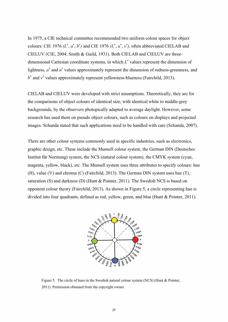
opponent colour theory (Fairchild, 2013). As shown in Figure 5, a circle representing hue is

divided into four quadrants, defined as red, yellow, green, and blue (Hunt & Pointer, 2011).

Figure 5. The circle of hues in the Swedish natural colour system (NCS) (Hunt & Pointer,

2011). Permission obtained from the copyright owner.

37

Device RGB colour systems (dRGB) appear to be similar to the CIE RGB system, but they

are specific to the characteristics of the primaries of devices. They were initially used in the

television and computer display industries. dRGB systems describe the relationship between

chromaticity and the colour stimuli generated by red, green and blue phosphors in a display

(Hunt & Pointer, 2011). The CMYK system is also a device colour space, specifically for

those devices that use subtractive colour mixing with more than three primary channels, such

as printers that use cyan, magenta, yellow, and black inks. To reproduce colours, colour space

inputs are transferred to device stimulus outputs, and this process is known as device

characterisation (Schanda, 2007). Sending a CMYK image to a CMYK printer is

straightforward, while sending it to a red-green-blue three primary projector requires the

device to mathematically transfer CMYK to dRGB, by assigning the colourant combinations

to dRGB triplets, which relate to the intensities of the three primary colour stimuli generated

by the projector. The conversion formulae vary from vendor to vendor (Hrehorova, Sharma,

& Fleming, 2006).

Although there are a variety of useful colour systems for different applications, the

fundamental principle underlying most of them is the specification of colour with three-

dimensional coordinates. Most colour systems can be categorized into three types: RGB

models, HSB models and opponent colour models.

2.6. Colour differences

Wyszecki proposed a method for quantifying colour differences by calculating the Euclidean

distance between two points in a coordinate system. This method was quickly accepted by

CIE (Schanda, 2007; Wyszecki & Stiles, 1982). The chromaticity difference between two

light sources can be specified by the Euclidean distance between the two sets of chromaticity

coordinates on the CIE 1976 (u’, v’) diagram, as:

∆𝑢9𝑣9 = F(𝑢G9 − 𝑢H9 )H + (𝑣G9 − 𝑣H9 )H (6)

where (u’1, v’1) and (u’2, v’2) are the chromaticity coordinates of two light sources. This was

used in the third experiment of this thesis to assess the colour differences (Du’v’) between the

reference light and test light at the end of each experimental trial.

38

The CIE also defined the colour difference (∆E*ab) for object colours in CIE 1976 (L*, a*, b*)

system (Ohta & Robertson, 2006; Schanda, 2007; Wyszecki & Stiles, 1982). Since then, the

CIELAB colour difference formula has been widely used. The original, and most widely

used, form of CIELAB colour difference formulae is:

∆𝐸JK∗ = F(𝐿G∗ − 𝐿H∗ )H + (𝑎G∗ − 𝑎H∗)H + (𝑏G∗ − 𝑏H∗)H (7)

Where (L1*, a1*, b1*) and (L2*, a2*, b2*) are the CIELAB coordinates of colour 1 and colour 2.

This equation was used in the fourth experiment to assess the colour differences (∆E*ab)

between the lower surfaces of target and test booths at the end of each trial.

However, CIELAB is not a truly uniform colour space (Fairchild, 2013; Melgosa et al.,

2017). Much work has been done to develop a more uniform colour space and more accurate

colour difference equations. The CIE Colour Appearance Model of 1997 (CIECAM97) was

succeeded, in 2002, by a simpler and more accurate model, CIECAM02 (Luo & Li, 2007). A

CIE technical committee is now working on CIECAM16 to replace CIECAM02.

Several different colour difference equations have been developed, including one proposed

by the Colour Measurement Committee (CMC) of the Society of Dyers and Colourists

(∆ECMC), one recommended by the CIE in 1994 (∆E94) and one recommended by the CIE in

2000, (∆E00), often referred to as DE2000. The CIE 1994 (∆E94) formula was designed to

correct the non-uniformity of CIELAB by weighting hue, chroma and lightness in different

proportions (Millward, 2009; Witt, 2007). CIE 1994 (∆E94) was further improved upon in the

development of CIE DE2000 (∆E00) which is the most mathematically complicated colour

difference formula (Millward, 2009). It introduces more weighting functions and parametric

factors. Weighting functions correct the non-uniformities of CIELAB and the parametric

factors account for the influences of experimental viewing conditions (CIE, 2001). Luo

(2004), Johnson (2006) and Habekost (2007) suggested that ∆E00 quantifies small perceived

colour differences more accurately than other equations (as cited in Millward, 2009). CIE

Technical Committee (TC) 1-55 concluded that, based on the existing visual datasets, various

modern colour spaces perform similarly in the quantification of colour differences. Thus, the

committee was unable to propose a new uniform colour space with a Euclidean colour-

39

difference formula to replace CIEDE2000 (CIE, 2016). However, the current CIE DE2000

colour difference equation is only recommended for small colour differences £5.0 CIELAB

units (Melgosa et al., 2017). When the colour difference is greater than five units

(∆E*ab >5.0), the discontinuity in CIE DE2000 colour-difference is not negligible (Sharma,

Wu, & Dalal, 2005; Sharma, Wu, Dalal, & Celik, 2004). In Millward’s experiment, five

colour difference equations (∆E*ab, ∆E94, ∆E00, ∆ECMC and ∆EDIN99) were compared to assess

which best correlates with perceived colour difference. Ten Pantone colour samples were

used as the reference colours. Each sample was compared with four other colour samples,

each of which had a colour difference of 6 units (∆E*ab =6.0±0.5). The results showed “there

is no clear winner for a colour difference equation that outperforms the rest” (Millward,

2009).

In another experiment investigating the threshold of acceptable colour difference for colour

reproduction in graphic arts, the performance of CIE 94 and CIE DE2000 were compared to

the original CIELAB colour difference formula (∆E*ab). Neither CIE 94 nor CIE DE2000

offered significant improvement in producing a uniform space than CIELAB. The CIELAB

differences were found to be quite consistent (Johnson & Green, 2006).

Generally speaking, it is unlikely that major improvements to the uniformity of colour spaces

will be developed without considerable complexity (Johnson & Green, 2006; CIE, 2016).

Those alternative colour spaces and colour-difference equations are generally considered to

not be necessary for relatively large colour differences (∆E*ab ≥5.0). CIELAB, which has

been widely used in basic and applied research since 1976 (Melgosa et al., 2017) can still be

used in research investigating colour differences greater than 5.0 ∆E*ab.

2.7. Lighting control interfaces

Much research has been conducted to improve users’ experience with LCSs by improving the

graphic design and content of user interfaces, as well as creating more tangible interactive

media. Researchers have found that users’ awareness of their everyday lighting conditions to

be low, although most participants considered lighting to be important. A traditional LCS was

only used when (a) the lighting was undesirable, (b) the improvement, after using the LCS,

was significant or (c) the effort required to use the LCS was relatively low. Interactive and

40

tangible interfaces could improve the sense of playfulness that users experience when

operating LCSs (Offermans, van Essen, & Eggen, 2014).

Dugar and Donn (2011) attempted to establish a framework for future studies on tangible

lighting control systems. They proposed that information processing within the human brain

can be classified in three systems: the perceptual system, the cognitive system and the motor

system. According to them, the two processes of perception are the physical reception of the

stimuli and the processing and interpretation of that reception. Cognition is the process of

presenting, sequencing, pacing and delegating information on lighting control interfaces

appropriately. The motor system includes the output as the human behavioural response

mainly involving bodily movement. They summarised three views of tangible interaction in

lighting environments, “a data-centred view, an expressive-centred view and a space-centred

view.” The data-centred view is from the HCI researchers’ perspective. For them, the design

of tangible user interfaces mainly focuses on collecting and utilizing digital data and clearly

representing the information. The expressive-centred view, which largely applies to industrial

designers, emphasises bodily interaction with objects, rather than the form and appearance of

products. The space-centred view focuses on creating interactions between spaces and people

by sensing users’ activities in the spaces (Dugar & Donn, 2011).

Chien and Mahdavi’s research explored the requirements of a user-interface system to

facilitate effective communication and interaction between building occupants and

environmental systems. Twelve products were compared across three categories (information

types, control options, hardware) with seven criteria: functional coverage, environmental

information feedback, intuitiveness, mobility, network, input, and output. They suggested

that high-tech interface products that offer “high functional coverage” (i.e. offers many

different functions) “imposes a large cognitive load on (new) users.” They suggest that

control commands should be intuitive and not overly complicated (Chien & Mahdavi, 2008).

Dugar et al. identified the characteristics of an ideal lighting control system by re-examining

real-life scenarios using the principles of interaction design. They studied users’ interaction

with four types of lighting control interfaces (pushbutton, rotary, slide dimmers, and screen-

based virtual interfaces) across six dimensions: appearance, grab-ability, accuracy,

responsiveness, learning speed and ease-of-use (Dugar, Donn, & Osterhaus, 2011). They

concluded that end-users preferred remote interfaces that provided the option of controlling

41

touch-screen-based iconographic representations of light intensities, light colours and lighting

scenes. Additionally, end-users desired rich interactive experiences with control interfaces.

High resolution interactive LCSs give users more options, but may lead to user dissatisfaction

due to complexity or extra effort required. This could reduce the frequency that users interact

with the system, minimizing the potential to save energy (Dugar & Donn, 2011).

After surveying 410 people in 14 office buildings in the United Kingdom, Moore et al. (2002)

concluded that occupants recognised the importance of personalised lighting control.

However, some occupants commented that the lighting control systems that they used

“lacked user friendliness.” In a recent study, Yılmaz et al. found that small increments (high

resolution) in a dimming system confused users (Yılmaz, Ticleanu, Howlett, King, &

Littlefair, 2016). Although researchers suggested that colour-tunable controls could enhance

occupants’ mood, performance etc., they also believe that occupants need to understand

better how to use a colour changing control system to achieve their desired effects (Yılmaz et

al., 2016).

A control interface for colour-tunable systems could be designed based on a dRGB system,

such that each dimension controls a channel of a primary colour. In an LED system, the three

control dimensions would control the luminous output of red, green and blue light

respectively. RGB interfaces are the simplest device-specific signals interfaces, with only

three channels, but some colour-tunable LED systems have seven or eight channels and can

provide an enormous number of colour options, such as ETC (ETC, 2016) and Telelumen

products (Telelumen, 2016). The simplest three-channel 8-bit systems can produce 16 million

different colours, while a more advanced system can offer up to 3 × 1038 options. These

products are usually controlled by computer software. They can mix colours using a variety

of models including, but not limited to, CIE chromaticity systems, HSB models and device-

specific models that directly control the signals sent to devices, such as DMX, to change the

intensity of each single colour channel. Although this type of control software can,

theoretically, provide any colour precisely, they are complicated for untrained, general users.

Dugar and Donn suggested that numerous switching or dimming options (high LCS

resolution) could lead to the selection of the wrong light level or create an undesirable

atmosphere, making the lighting “annoying and tedious” (Dugar & Donn, 2011).

42

Some colour control interfaces of commercial products, such as the To Be Touched® from

Philips lighting, are based on a design modified from the HSB system and are similar to a

conventional artistic colour wheel. A typical design of this type control interface is shown in

Figure 6. These interface designs are assumed to be better understood by the general public

than RGB interfaces. However, there is little publically available empirical evidence on the

usability of the different colour specification interfaces.

Figure 6. A typical control interface design based on a colour wheel, modified from the HSB

system.

Another common design is a combination of a colour wheel based on HSB and additional

sliders, as shown in Figure 7. For instance, the colour-tunable product, LIFX, uses this type

of design (LIFX, 2017). Manufacturers usually select the labels and resolutions of the control

dimensions. For instance, “colour”, shown in Figure 7, refers to the control of saturation. The

smallest magnitude of change is 1 %. However, there is no available empirical data to suggest

that 1 % is an optimal resolution for either saturation or brightness. Although some large

companies may conduct research on the usability of LCSs, the research results are usually

confidential and not disseminated.

43

Figure 7. A typical control interface combining sliders with a colour wheel based on the HSB

system.

Although the comparison of colour mixing systems for a colour specification interface is a

relatively new topic in the lighting industry, it has been studied systematically for televisions

and computer displays, which require accurate colour specification.

Schwarz, Cowan and Beatty found that it is difficult for users to specify their desired colours

when displays provide 16 million colour options. In an experiment, they compared the

usability of RGB, luma, in-phase, quadrature (YIQ), CIELAB, hue, saturation, value (HSV)

and opponent colour models for displays (Schwarz, Cowan, & Beatty, 1987). For

inexperienced users, the RGB control interface allowed the fastest completion of colour-

matching tasks, but the matching results were not very accurate. The HSV interface was the

slowest, but the most accurate (Schwarz et al., 1987).

A conflicting result was reported earlier (Murch, 1984), which found that a hue, saturation,

lightness (HSL) interface was the most efficient one for inexperienced users (as cited in

Douglas & Kirkpatrick, 1996). However, detailed data was not published. Douglas and

Kirkpatrick conducted a colour-matching experiment and reported that no significant

difference in colour matching accuracy was observed between RGB and HSV colour models

when the position of current colour in the colour space was shown to the subjects (Douglas &

Kirkpatrick, 1996).

44

Hughes and Foley claimed that an interface based on the RGB system is not ideal as a colour-

selection tool for a computer. This is partly because it is better suited to “material colours but

not coloured lights, where the intensity can be arbitrarily large.” The authors further

suggested two alternative interfaces: the HSV interface and the HLS interface. The RGB

model is described as a hardware-oriented model, while the HSV model is user-oriented

(Hughes & Foley, 2014). Fairchild suggested that, for image editing, three control

dimensions - hue, chroma and lightness - is more intuitive for untrained users to manipulate

the image colours than device dependent colour spaces, such as dRGB and CMYK (Fairchild,

2013). However, it is not clear whether the results for displays and image editing are also

applicable to lighting.

Beigpour and Pedersen (2015) compared RGB and HSV interfaces in a recent experiment.

The researchers instructed participants to match the colour of a Philips Hue lamp with a

colour displayed on a computer screen. When using the HSV interface, participants matched

colours more rapidly, but less accurately. It is worth noting that in this experiment, instead of

matching the colours displayed on two identical devices, participants matched the colours

between a lamp and a computer screen.

Research on colour selection models in the display industries started much earlier than in the

lighting industry. There are still some ongoing debates, and no well-accepted result has been

forthcoming. Even if their results were consistent, they might not be suitable to apply to

lighting products. Computer displays, which are defined as self-luminous objects in

colorimetry, are different from light sources for colorimetry purposes. The colorimetric

formulae used for displays (self-luminous objects) differ from those for the chromaticity of

light (Schanda, 2007).

2.8. Usability assessment

Usability is a term widely used to describe the quality of use in the field of interface design.

Nielsen (1994) stated that usability as an indeterminable concept, but is related to several

measurable parameters, such as the time to complete a task, number of user errors, etc.

ISO 9241 Part 11 (Guidance on usability) defined usability as the extent to which a product

can be used to achieve goals in three areas: effectiveness, efficiency and satisfaction (ISO,

45

1998). Effectiveness can be measured by the accuracy and completeness with which users

achieve goals. Indicators of efficiency include task completion time, learning time and the

resources expended to achieve the goals. Satisfaction is the users’ positive attitudes towards

the use of the system. Effectiveness and efficiency are more objective and easier to measure.

This might be part of the reason that some earlier studies only considered effectiveness and

efficiency when assessing usability.

Hassenzahl (2001) pointed out that measurement of user satisfaction in some earlier studies

might have actually tested users’ recognition of design objectives. He further argued that

efficiency and effectiveness cannot guarantee user satisfaction. The findings of experiments

carried out by Nielsen and Levy (1994) provided evidence. Although there was a strong

correlation between users’ task performance (measured by the efficiency and effectiveness)

and satisfaction, in 25 % of the cases, the participants were most satisfied with the system

with which their performance was not the best.

Another debate is whether these three aspects are equally weighted in the assessment of

usability. Researchers investigated the correlation between effectiveness, efficiency and

satisfaction. Sauro and Kindlund (2005) used four metrics to represent these three aspects.

They measured task completion and numbers of errors (effectiveness), task time (efficiency),

and satisfaction ratings from questionnaires. They concluded that these metrics were equally

weighted. Nevertheless, other researchers’ findings have not supported this conclusion. Park

and his colleagues set up a model to evaluate the usability of interface design (Park & Lim,

1999). In this model, the weights of the three criteria were 0.32, 0.28, 0.40 for effectiveness,

efficiency and satisfaction respectively. These weights were established from the user testing

data, results of questionnaire and experts’ judgments. They stated that the prioritisation of the

dimensions should be reviewed by experts, as the users did not have sufficient experience to

evaluate their relative importance. This involvement of experts’ subjective opinions might be

valuable, but are also at risk of expert bias.

Although there is a vast literature on the design of user satisfaction questionnaires and some

of them have been accepted as standardized questionnaires, few studies measuring

satisfaction have focused on LCSs. Tullis and Stetson compared five questionnaires for

46

assessing website usability: four standard questionnaires (SUS 4, QUIS 5, CSUQ 6 and

Microsoft’s product reaction cards) and one questionnaire designed by their own lab. They

recommended two questionnaires after the comparison: SUS and CSUQ (Tullis & Stetson,

2004). Sauro and Kindlund (2005) also reviewed several questionnaires, such as the SUMI 7

and PSSUQ 8, and then set up their own model to standardize usability metrics into a single

score. Though their model might not be generalisable to lighting, the simple questionnaire

used in their experiment can be used in this project. The three-item after-scenario

questionnaire (ASQ) was originally from Lewis’ paper, and is widely used in computer

usability assessments. This questionnaire only has three questions and it deemed to have

“acceptable psychometric properties of reliability, sensitivity and concurrent validity”

(Lewis, 1991). Moreover, their ASQ did not include any specific task related questions, so it

can be used with confidence in similar usability studies.

4 SUS: system usability scale 5 QUIS: questionnaire for user interface satisfaction 6 CSUQ: computer system usability questionnaire 7 SUMI: the software usability measurement inventory 8 PSSUQ: post-study system usability questionnaire

47

References

Al-Rasheed, A. S. (2015). An experimental study of gender and cultural differences in hue

preference. Frontiers in Psychology, 6(30).

Aslam, M. M. (2006). Are you selling the right colour? A cross-cultural review of colour as a

marketing cue. Journal of Marketing Communications, 12(1), 15-30.

Barlow, H. B. (1957). Increment thresholds at low intensities considered as signal/noise

discriminations. The Journal of Physiology, 136 (3), 469-488.

Beigpour, S., & Pedersen, M. (2015). Color Play: Gamification for Color Vision Study. Paper

presented at the Color and image. Midterm Meeting of the International Colour

Association (AIC), Tokyo, Japan.

Blackwell, H. R. (1946). Contrast thresholds of the human eye. Journal of the Optical

Society of America, 36 (11) 624-643.

Brainard, G. C., Hanifin, J. P., Greeson, J. M., Byrne, B., Glickman, G., Gerner, E., &

Rollag, M. D. (2001). Action spectrum for melatonin regulation in humans: evidence

for a novel circadian photoreceptor. Journal of Neuroscience, 21(16), 6405-6412.

Brendel, M., Kruse, A., Jönen, H., Hoffmann, L., Bremers, H., Rossow, U., & Hangleiter, A.

(2011). Auger recombination in GaInN/GaN quantum well laser structures. Applied

Physics Letters, 99(3), 031106. doi:10.1063/1.3614557

Brown, S. W., Santana, C., & Eppeldauer, G. P. (2002). Development of a tunable LED-

based colorimetric source. Journal of Research of the National Institute of Standards

and Technology, 107(4), 363.

Cajochen, C. (2007). Alerting effects of light. Sleep medicine reviews, 11(6), 453-464.

Camgöz, N., Yener, C., & Güvenç, D. (2002). Effects of hue, saturation, and brightness on

preference. Color Research & Application, 27(3), 199-207.

Chang, M., Das, D., Varde, P. V., & Pecht, M. (2012). Light emitting diodes reliability

review. Microelectronics Reliability, 52(5), 762-782.

doi:10.1016/j.microrel.2011.07.063

Chien, S., & Mahdavi, A. (2008). Evaluating interface designs for user-system interaction

media in buildings. Advanced Engineering Informatics, 22(4), 484-492.

doi:10.1016/j.aei.2008.06.004

Cho, J., Park, J. H., Kim, J. K., & Schubert, E. F. (2017). White light-emitting diodes:

History, progress, and future. Laser & Photonics Reviews.

48

Commission Internationale de l’Eclairage (CIE). (2001). CIE 142-2001: Improvement to

industrial colour-difference evaluation. In: CIE Central Bureau.

Commission Internationale de l’Eclairage (CIE). (2004). Colorimetry, 3rd edition (CIE

15:2004 Technical Report).

Commission Internationale de l’Eclairage (CIE). (2016). Recommended method for

evaluating the performance of colour-difference formulae (No. 217:2016). Vienna,

Austria: CIE.

Cooper, N. R., Croft, R. J., Dominey, S. J. J., Burgess, A. P., & Gruzelier, J. H. (2003).

Paradox lost? Exploring the role of alpha oscillations during externally vs. internally

directed attention and the implications for idling and inhibition hypotheses.

International Journal of Psychophysiology, 47(1), 65-74.

doi:https://doi.org/10.1016/S0167-8760(02)00107-1

Cornsweet, T. N., & Pinsker, H. M. (1965). Luminance discrimination of brief flashes under

various condition of adaption. The Journal of Physiology. (1965), 176, 294-310.

Cree. (2016). LED Color Mixing: Basics and Background. Retrieved from

http://www.cree.com/led-components/media/documents/LED_color_mixing.pdf

Cubukcu, E., & Kahraman, I. (2008). Hue, saturation, lightness, and building exterior

preference: An empirical study in Turkey comparing architects’ and nonarchitects’

evaluative and cognitive judgments. Color Research & Application, 33(5), 395-405.

CVRL. (2016). Colour & Vision database: Colour Matching Functions. Retrieved from

http://www.cvrl.org/

DeCusatis, C. (1997). Handbook of applied photometry: American Inst. of Physics.

Denicholas, J. (2017). Dimming. Handbook of Advanced Lighting Technology, 445-464.

De Valois, R. L., & De Valois, K. K. (1993). A multi-stage color model. Vision Research,

33(8), 1053-1065.

deVries, H. (1943). The quantum character of light and its bearing upon threshold of vision,

the differential sensitivity and visual acuity of the eye. Physical Review X, no.7.

Douglas, S., & Kirkpatrick, T. (1996). Do color models really make a difference? Paper

presented at the Proceedings of the SIGCHI conference on Human factors in

computing systems.

Dugar, A. M., & Donn, M. R. (2011). Tangible intervention- Improving the effectiveness of

lighting control systems. Lighting Research & Technology. 2011; 43: 381–393.

49

Dugar, A. M., Donn, M. R., & Osterhaus, W. (2011). Tangible lighting controls—Reporting

end- users’ interactions with lighting control interfaces. LEUKOS, 08, P 123–136.

doi:10.1582/leukos.2011.08.02.003

Dyble, M., Narendran, N., Bierman, A., & Klein, T. (2005). Impact of dimming white LEDs:

chromaticity shifts due to different dimming methods. Paper presented at the Fifth

international conference on solid state lighting.

ETC. (2016). Source Four. Lighting Fixtures. Retrieved from

https://www.etcconnect.com/Products/Lighting-Fixtures/Source-Four/Source-

Four/Features.aspx

Fairchild, M. D. (2013). Color appearance models: John Wiley & Sons.

Farell, B., & Pelli, D. G. (1999). Psychophysical methods, or how to measure a threshold and

why. Vision research: A practical guide to laboratory methods, 5, 129-136. New

York: Oxford University Press.

Farrell, T. (2009). Colour for Architecture Today (T. P. B. Mikellides Ed.). New York:

Taylor & Francis Ltd.

Fechner, G. T. (1851). Outline of a new principle of mathematical psychology (1851).

Psychological Research, 49(4), 203-207.

George, B., & James, T. (2012). Lighting conditions in sustainable buildings: results of a

survey of users’ perceptions. Architectural Science Review, 55(2), 102-109.

doi:10.1080/00038628.2012.667941

Gu, Y., Narendran, N., Dong, T., & Wu, H. (2006). Spectral and luminous efficacy change of

high-power LEDs under different dimming methods. Paper presented at the Sixth

International Conference on Solid State Lighting.

Hassenzahl, M. (2001). The Effect of Perceived Hedonic Quality on Product Appealingness.

International Journal of Human-Computer Interaction, 13(4), 481-499.

doi:10.1207/s15327590ijhc1304_07

Hecht, S., Shlaer, S., & Pirenne, A. H. (1942). Energy, Quanta, and Vision. General

Physiology 25: 819–840.

Holmes, R., Victora, M., Wang, R. F., & Kwiat, P. G. (2017). Measuring temporal

summation in visual detection with a single-photon source. Vision research, 140, 33-

43.

Honig, L. M. (2009). Physiological and psychological response to colored light (Doctoral

dissertation, Saybrook University).

50

Hrehorova, E., Sharma, A., & Fleming, P. D. (2006). Color reproduction studies in RGB and

CMYK workflows using inkjet printer drivers and RIPs. Paper presented at the Proc.

58th TAGA Annual Technical Conference, Vancouver, British Columbia.

Hughes, J. F., & Foley, J. D. (2014). Computer graphics: principles and practice: Pearson

Education.

Hunt, R. W. G., & Pointer, M. R. (2011). Measuring colour: John Wiley & Sons.

Hurlbert, A. C., & Ling, Y. (2007). Biological components of sex differences in color

preference. Current Biology, 17(16), R623-R625.

doi:https://doi.org/10.1016/j.cub.2007.06.022

International Organization for Standardization (ISO) (1998). ISO 9241-11: Ergonomic

Requirements for Office Work with Visual Display Terminals (VDTs): Part 11:

Guidance on Usability.

Ji, P. F., & Moon, C.-H. (2013). Change of effective thermal resistance of LED package

according to an input current level. Solid-State Electronics, 85, 1-5.

Johnson, A., & Green, P. (2006). The colour difference formula CIEDE2000 and its

performance with a graphic arts data set. TAGA Journal of Graphic Technology, 2,

59-71.

Johnson, A., & Toffanin, P. (2012). Self-chosen colored light induces relaxation. Paper

presented at the Proceedings of experiencing light 2012: international conference on

the effects of light on wellbeing.

Julian, W., & Lumascape. (2016). The Sydney opera house concert hall celebrates two years

of LEDs. Lighting, 36(4), 26-27.

Kim, M., Schubert, M. F., Dai, Q., Kim, J. K., Schubert, E. F., Piprek, J., & Park, Y. (2007).

Origin of efficiency droop in GaN-based light-emitting diodes. Applied Physics

Letters, 91(18), 183507. doi:10.1063/1.2800290

Kim, S. Y., & Kim, J. J. (2007). Influence of light fluctuation on occupant visual perception.

Building and Environment, 42(8), 2888-2899.

Krueger, L. E. (1989). Reconciling Fechner and Stevens: Toward a unified psychophysical

law. Behavioral and Brain Sciences, 1989.

Lewis, J. R. (1991). Psychometric evaluation of an after-scenario questionnaire for computer

usability studies- the ASQ. ACM Sigchi Bulletin, 23(1), 78-81.

LIFX. (2017). LIFX Wi-Fi LED Lights. Retrieved from

https://www.lifx.com.au/collections/featured-products

51

LM-79-08, I. (2008). Electrical and Photometric Measurements of Solid-State Lighting

Products. In: Illuminating Engineering Society.

Luo, R. M., & Li, C. (2007). CIE color appearance models and associated color spaces. In J.

Schanda (Ed.), Colorimetry: Understanding the CIE System: John Wiley & Sons.

MacAdam, D. L. (1935). Maximum Visual Efficiency of Colored Materials. Journal Of The

Optical Society Of America, 25(11), 361-367.

MacAdam, D. L. (1939). Representation of color tolerance on the chromaticity diagram. The

American Journal of Psychology, 52(3) 412-418.

MacAdam, D. L. (1942). Visual Sensitivities to Color Differences in Daylight. Journal Of

The Optical Society Of America, 32(5), 247-274.

Major, M. (2009). Architectural light and colour as a source of inspiration: an apporoach to

the use of colour. In T. P. B. Mikellides (Ed.), Colour for Architecture Today (151-

158). New York: Taylor & Francis Ltd.

Martin, S., Sameer, C., Kyu, K. J., Fred, S. E., Daniel, K., Mary, C., . . . Michael, B. (2007).

Effect of dislocation density on efficiency droop in GaInN⁄GaN light-emitting diodes.

Applied Physics Letters, 91(23), 231114. doi:10.1063/1.2822442

McManus, I., Jones, A. L., & Cottrell, J. (1981). The aesthetics of colour. Perception, 10(6),

651-666.

Melgosa, M., Gómez-Robledo, L., García, P., Morillas, S., Fernández-Maloigne, C., Richard,

N., . . . Cui, G. (2017). Color-quality control using color-difference formulas:

progress and problems. Paper presented at the Third International Conference on

Applications of Optics and Photonics.

Millward, S. (2009). Color difference equations and their assessment. Test Target, J 9, 19-26.

Moore, T., Carter, D., & Slater, A. (2002). User attitudes toward occupant controlled office

lighting. Lighting Research & Technology, 34(3), 207-216.

Murch, G. M. (1984). The effective use of color: Cognitive principles (Vol. 8): Tekniques.

Narra, P., & Zinger, D. S. (2004). An effective LED dimming approach. Paper presented at

the Industry Applications Conference, 2004. 39th IAS Annual Meeting. Conference

Record of the 2004 IEEE.

Narukawa, Y., Ichikawa, M., Sanga, D., Sano, M., & Mukai, T. (2010). White light emitting

diodes with super-high luminous efficacy. Journal of Physics D: Applied Physics,

43(35), 354002.

Networks, D. (2010). Occupancy sensors deliver lighting on demand. Daintree Networks,

2010.

52

Nielsen, J., & Levy, J. (1994). Measuring usability: preference vs. performance.

Communications of the ACM, 37(4), 66-75. doi:10.1145/175276.175282

Nielsen, J. (1994). Usability engineering: Elsevier.

Norton, T. T., Corliss, D. A., & Bailey, J. E. (2002). The psychophysical measurement of

visual function (Vol. 362): Butterworth-Heinemann Woburn.

Offermans, S. A. M., van Essen, H. A., & Eggen, J. H. (2014). User interaction with

everyday lighting systems. Personal and Ubiquitous Computing, 18(8), 2035-2055.

doi:10.1007/s00779-014-0759-2

Ohta, N., & Robertson, A. (2006). Colorimetry: fundamentals and applications: John Wiley

& Sons.

Ou, L.-C., Luo, M. R., Woodcock, A., & Wright, A. (2004a). A study of colour emotion and

colour preference. Part I: Colour emotions for single colours. Color Research &

Application, 29(3), 232-240. doi:10.1002/col.20010

Ou, L.-C., Luo, M. R., Woodcock, A., & Wright, A. (2004b). A study of colour emotion and

colour preference. Part II: Colour emotions for two-colour combinations. Color

Research & Application, 29(4), 292-298. doi:10.1002/col.20024

Ou, L.-C., Luo, M. R., Woodcock, A., & Wright, A. (2004c). A study of colour emotion and

colour preference. Part III: Colour preference modeling. Color Research &

Application, 29(5), 381-389. doi:10.1002/col.20047

Palmer, S. E., & Schloss, K. B. (2010). An ecological valence theory of human color

preference. Proceedings of the National Academy of Sciences, 107(19), 8877-8882.

doi:10.1073/pnas.0906172107

Park, K. S., & Lim, C. H. (1999). A structured methodology for comparative evaluation of

user. International Journal of Industrial Ergonomics 23, 379—389.

Pattison, P. M., Hansen, M., & Tsao, J. Y. (2017). LED lighting efficacy: Status and

directions. Comptes Rendus Physique.

Pelli, D. G., & Farell, B. (1995). Psychophysical methods. Handbook of optics, 3, 3.1-3.12.

Philips. (2010). Optibin Technology Overview. Retrieved from

http://www.colorkinetics.com/ls/guides-brochures/PCK-Technology-Overview-

Optibin.pdf

Philips. (2018b). MASTER TL5 HE 28W/840 SLV/40. Retrieved from

http://www.lighting.philips.com.au/prof/conventional-lamps-and-tubes/fluorescent-

lamps-and-starters/tl5/master-tl5-high-efficiency/927926584055_EU/product

53

Priluck Grossman, R., & Wisenblit, J. Z. (1999). What we know about consumers’ color

choices. Journal of Marketing Practice: Applied Marketing Science, 5(3), 78-88.

Sachs, H., Nadel, S., Amann, J. T., Tuazon, M., Mendelsohn, E., Rainer, L., . . . Adelaar, M.

(2004). Emerging energy-saving technologies and practices for the buildings sector as

of 2004. American Council for an Energy-Efficicent Economy (ACEEE), Davis

Energy Group, and Marbek Resource Consultants, Washington, DC, Report (A042),

214-246.

Saguatti, D., Bidinelli, L., Verzellesi, G., Meneghini, M., Meneghesso, G., Zanoni, E., . . .

Hahn, B. (2012). Investigation of Efficiency-Droop Mechanisms in Multi-Quantum-

Well InGaN GaN Blue Light-Emitting Diodes. IEEE Transactions on Electron

Devices, 59(5).

Sauro, J., & Kindlund, E. (2005). A Method to Standardize Usability Metrics. CHI 2005/

Paper: Methods & Usability.

Schanda, J. (2007). Colorimetry: Understanding the CIE System (J. Schanda Ed.): John

Wiley & Sons, Inc.,.

Schwarz, M. W., Cowan, W. B., & Beatty, J. C. (1987). An experimental comparison of

RGB, YIQ, LAB, HSV, and opponent color models. ACM Transactions on Graphics

(TOG), 6(2), 123-158.

Sharma, G., Wu, W., & Dalal, E. N. (2005). The CIEDE2000 color-difference formula:

Implementation notes, supplementary test data, and mathematical observations. Color

Research & Application, 30(1), 21-30.

Sharma, G., Wu, W., Dalal, E. N., & Celik, M. U. (2004). Mathematical discontinuities in

CIEDE2000 color difference computations. Paper presented at the Color and Imaging

Conference.

Smith, T., & Guild, J. (1931). The CIE colorimetric standards and their use. Transactions of

the Optical Society, 33(3), 73.

Spitschan, M., Lucas, R. J., & Brown, T. M. (2017). Chromatic clocks: Color opponency in

non-image-forming visual function Review. Neuroscience & Biobehavioral Reviews.

Stevens, S. S. (1961). To honor Fechner and repeal his law. Science, 133, 80-86.

doi:10.1126/science.133.3446.80

Stiles, W., & Burch, J. (1955). Interim report to the Commission Internationale de l'Eclairage,

Zurich, 1955, on the National Physical Laboratory's investigation of colour-matching

(1955). Optica Acta: International Journal of Optics, 2(4), 168-181.

54

Tao, Y., Wang, S., Chen, Z., Gong, Z., Xie, E., Chen, Y., . . . Gu, E. (2012). Size effect on

efficiency droop of blue light emitting diode. Physica Status Solidi (c), 9(3-4), 616-

619. doi:10.1002/pssc.201100483

Telelumen. (2016). Products. Retrieved from http://www.telelumen.com/products2.html

Thapan, K., Arendt, J., & Skene, D. J. (2001). An action spectrum for melatonin suppression:

evidence for a novel non-rod, non-cone photoreceptor system in humans. The Journal

of Physiology, 535(1), 261-267.

Tonello, G. (2008). Seasonal affective disorder: Lighting research and Environmental

psychology. Lighting Research & Technology, 40(2), 103-110.

Tullis, T. S., & Stetson, J. N. (2004). A comparison of questionnaires for assessing website

usability. Paper presented at the Usability Professional Association Conference.

Turrell, J. (2017). Architectural light. Retrieved from

http://jamesturrell.com/work/type/architectural-light/

Viénot, F., Coron, G., & Lavédrine, B. (2011). LEDs as a tool to enhance faded colours of

museums artefacts. Journal of Cultural Heritage, 12(4), 431-440.

Wade, N. J., & Swanston, M. (2013). Visual perception: An introduction: Psychology Press.

Watson, D., Clark, L. A., & Tellegen, A. (1988). Development and validation of brief

measures of positive and negative affect: the PANAS scales. Journal of Personality

and Social Psychology, 54(6), 1063.

Williams, A., Atkinson, B., Garbesi, K., Page, E., & Rubinstein, F. (2012). Lighting Controls

in Commercial Buildings. LEUKOS, 8(3), 161-180.

doi:10.1582/leukos.2012.08.03.001

Windhorst, U., & Johansson, H. (2012). Modern techniques in neuroscience research:

Springer Science & Business Media.

Witt, K. (2007). CIE Color Difference Metrics. In J. n. Schanda (Ed.), Colorimetry :

Understanding the CIE system (pp. 79-100). Canada: John Wiley & Sons, Inc.,.

Wood, M. (2010). Many Shades of White. Stage Directions, 23.

Woolfson, M. M. (2016). Colour: how we see it and how we use it: London ; Hackensack,

NJ : World Scientific Publishing (UK) Ltd.,.

Wright, W. D. (1929). A re-determination of the trichromatic coefficients of the spectral

colour. Transactions of the Optical Society.

Wyszecki, G., & Stiles, W. S. (1982). Color science (Vol. 8): Wiley New York.

55

Yılmaz, F., Ticleanu, C., Howlett, G., King, S., & Littlefair, P. (2016). People-friendly

lighting controls–User performance and feedback on different interfaces. Lighting

Research & Technology, 48(4), 449-472.

56

Chapter 3. Dimming curve based on the detectability and

acceptability of illuminance differences

57

Dimming curve based on the detectability and acceptability of illuminance differences

Wenye Hu1,* and Wendy Davis1,2 1Faculty of Architecture, Design and Planning, The University of Sydney, NSW 2006, Australia

2wendy.davis@sydney.edu.au * wehu7684@uni.sydney.edu.au

Abstract: In a psychophysical forced-choice experiment, observers’ ability to detect illuminance differences was found to be 7.4% of the initial illuminance. When matching the illuminance of one space with another, observers’ acceptance of illuminance differences was 17.8% to 19.1%. Lighting control systems with resolutions between 14.8% and 17.7% were found to have greater usability than others. A new approach to step-dimming leverages knowledge of the detectability and acceptability of illuminance differences, as well as usability, to reduce lighting energy consumption. This method can reduce lighting energy consumption more than continuous dimming.

©2016 Optical Society of America

OCIS codes: (220.2945) Illumination design; (330.7310) Vision; (350.4600) Optical engineering.

References and links

1. Y. Akashi and J. Neches, “Detectability and acceptability of illuminance reduction for load shedding,” J. Illum. Eng. Soc. 33(1), 3–13 (2004).

2. Y. Akashi and P. R. Boyce, “A field study of illuminance reduction,” Energy Build. 38(6), 588–599 (2006). 3. T. Shikakura, H. Morikawa, and Y. Nakamura, “Research on the perception of lighting fluctuation in a luminous

offices environment,” J.Illum. Engng. Inst. Jpn. 85(5), 346–351 (2001). 4. Philips, “An introduction to DALI” http://www.lighting.philips.com.au/v2/static/usr/auto-grab/An Introduction

to DALI.pdf. 5. M. F. Schubert, S. Chhajed, J. K. Kim, E. F. Schubert, D. D. Koleske, M. H. Crawford, S. R. Lee, A. J. Fischer,

G. Thaler, and M. A. Banas, “Effect of dislocation density on efficiency droop in GaInN/GaN light-emitting diodes,” Appl. Phys. Lett. 91(23), 231114 (2007).

6. C. Weng, “Advanced thermal enhancement and management of LED packages,” Int. Commun. Heat. Mass. 36(3), 245–248 (2009).

7. H. R. Blackwell, “Contrast thresholds of the human eye,” J. Opt. Soc. Am. 36(11), 624–643 (1946). 8. H. B. Barlow, “Increment thresholds at low intensities considered as signal/noise discriminations,” J. Physiol.

136(3), 469–488 (1957). 9. W. H. Ehrenstein and A. Ehrenstein, “Psychophysical methods” in Modern Techniques in Neuroscience

Research (Springer Berlin Heidelberg, 1999), 1211–1241. 10. T. Shikakura, H. Morikawa, and Y. Nakamura, “Perception of lighting fluctuation in office lighting

environment,” J. Light Vis. Environ. 27(2), 75–82 (2003). 11. ISO, “Ergonomic requirements for office work with visual display terminals (VDTs),” in Part 11: Guidance on

usability ISO 9241–11:1998, ISO, (1998) 12. J. Sauro and E. Kindlund, “A method to standardize usability metrics into a single score,” in Proceedings of the

SIGCHI Conference on Human Factors in Computing Systems (ACM, 2005), 401–409. 13. N. Jakob and L. Jonathan, “Measuring usability: preference vs. performance,” Commun. ACM 37(4), 66–75

(1994). 14. T. T. Norton, D. A. Corliss, and J. E. Bailey, The Psychophysical Measurement of Visual Function (Butterworth-

Heinemann, 2002). 15. D. Marcus, K. S. Hickcox, E. Bear, J. P. Freyssinier, and N. Narendran, “ASSIST recommends: dimming: a

technology-neutral definition” (LRC, 2013). 16. IESNA, The IESNA Lighting Handbook, 10 ed. (2011). 17. Lutron, “Measured light vs. perceived light”

http://www.lutron.com/TechnicalDocumentLibrary/Measured_vs_Perceived.pdf 18. Y. Narukawa, J. Narita, T. Sakamoto, T. Yamada, H. Narimatsu, M. Sano, and T. Mukai, “Recent progress of

high efficiency white LEDs,” Phys. Status Solidi., A Appl. Mater. Sci. 204(6), 2087–2093 (2007).

58

1. Introduction

Previous research has investigated strategies for reducing the energy consumed by lighting by reducing the illuminance of electrically lit spaces [1, 2]. Research suggests that occupants cannot detect illuminance reductions of up to 20% [3]. Although earlier research results were technology-neutral, much of this research was conducted with fluorescent lights. Dimmable fluorescent products in the market are fluorescent luminaires with electronic dimmable ballasts. The relative high cost of fluorescent dimming ballasts prevented widespread adoption of those research findings in real illumination applications. Dimmable fluorescent systems were historically used in high-end commercial spaces.

With the development of dimmable light-emitting diodes (LEDs) and digital control technologies, dimming in commercial spaces has become easier and more economical. LED dimming technology is well-established and commercially available, as long as users choose LED lamps, drivers and control systems compatible with each other. Dimmable LED lighting systems have already been used in a large number of lighting application areas to provide general lighting. Additionally, the increasing need for sustainable building design encourages increased use of dimmable LEDs with automatic control systems and daylight harvesting systems. Those advanced control systems could be designed with very high resolution, with “resolution” referring to the smallest change that can be produced by a lighting control system (LCS). Many lighting products are compatible with the DALI (Digital Addressable Lighting Interface) control protocol, which provides 256 levels of brightness between off and the maximum level [4].

If a lighting control system was to automatically reduce illuminance slightly, such that the change was either undetectable or at least acceptable to the user, energy consumption would be reduced in two ways: the power driving the light source would be reduced and the LEDs would exhibit higher efficacy, from reduced current and thermal droop. LED current droop, which is the reduction of luminous efficacy with increases in current, means that LEDs operate with relatively low efficacy at the relatively high drive currents needed for illumination applications [5]. Since increased LED junction temperature also leads to a reduction in internal quantum efficiency, reducing the heat generated by the LEDs would also increase efficacy [6]. When users of lighting control systems increase illuminance in a space, the luminous efficacy of the LED lighting system is reduced. When users decrease illuminance, the efficacy of the lighting is increased.

Thus, attention has been drawn back to illuminance reduction again for energy conservation. However, the development of lighting control systems that operate in this manner requires a better understanding of users’ ability to detect differences in illumination, their acceptance of illuminance differences, and their satisfaction with LCSs of various resolutions. This project combines psychophysical experiments with a questionnaire to investigate the detectability and acceptability of illuminance differences and applies the results in the design of lighting control systems, by proposing a series of dimming curves.

2. Previous studies

2.1 Detectability

Numerous previous works explored the human visual system’s ability to detect differences in brightness. Initial research, dating back to as early as the 1940s, in this field mainly focused on human visual perception [7, 8]. Most research directly applied to lighting on this topic is more recent. Akashi and Neches proposed a solution for load shedding by reducing illuminance. They investigated four dimming curves and reported that “dimming curvature,” which refers to the shape of the dimming curve, “has little influence on the detection of illuminance reduction” and that 50% of their experimental participants could detect a 15% reduction of the initial illuminance [1]. In their experiment, participants were asked whether the illuminance increased, decreased or remained the same. This method, although direct and

59

efficient, relies heavily on the participants’ subjective reports of what they perceived. When participants reported the detection of change, they were usually very confident with their judgments. This means that an observer’s ability to detect differences was likely underestimated with this method. Psychophysicists have found that, by using forced-choice method, many observers could detect very weak signals, which they claimed they could not detect [9].

Recently, a study conducted by Shikakura’s team, on the “minimum ratio of perceiving fluctuation” systematically examined the detectability of illuminance differences [10]. They reported that the detectability of illuminance decreases and illuminance increases were 8% and 6% respectively, when no visual task was involved in the experiment. The first experiment in this project suffers from two issues: firstly, a neutral response option - “cannot determine”- was provided, meaning that participants were not required to make a positive or negative judgment. However, psychophysicists have found that some stimuli, which observers claim cannot be detected, can in fact be detected correctly in forced choice experiments. The authors pointed out that the stimulus detection threshold was probably overestimated by offering the neutral option. They suggested the use of a classical forced-choice psychophysical method, in which participants would be forced to choose a positive or negative response without a neutral option [9]. Another issue is the possibility of the false detection of stimuli in Shikakura’s experiment. When participants reported changes in illuminance without indicating whether it was increased or decreased, there was no way to determine whether observers’ reports were representative of their percepts or the result of response errors. Shikakura’s team noticed this issue and improved their second experiment by asking participants whether illuminance was increased or decreased. All false detections were treated as errors when analyzing the data.

2.2 Acceptability

Unlike the classic studies of detection, which date from over a hundred years ago, research on users’ acceptance of various lighting conditions gained more attention in recent years. Researchers reported that illuminance reductions of up to 30% could be accepted by occupants [1–3]. Akashi and Neches suggested that 50% and 80% participants accepted illuminance reductions of up to 40% and 20%, respectively. They stated again that the shape of dimming curve had little impact on the acceptability of illuminance reductions [10]. In a field study on office lighting, author suggested that illuminance reductions of up to one third of the initial illuminance had no long-term impact on users’ satisfaction [2]. However, most results about user acceptance use verbal reports of participants or subjective ratings. Well controlled psychophysical experiments would strengthen the conclusions that could be drawn.

Resolution, which is the brightness difference produced by each control input action, is essential for every LCS. For an efficient and user-friendly LCS, the value of resolution should be between the users’ illuminance difference detection threshold and acceptance threshold. Therefore, user acceptability of the illuminance differences, which is constrained the LCS resolution, is of equal importance. The concept of usability is widely used in studies of human-computer interaction (HCI) and can be used to measure user acceptance of the resolution of LCSs.

According to ISO 9241 Part 11-Guidance on usability, usability is defined as “the extent to which a product can be used to achieve goals in three areas: effectiveness, efficiency and satisfaction” [11]. It is a property of any interactive digital technology, revealing whether the system is simple and pleasant to use. Accuracy of task completion can be used to measure effectiveness, while efficiency can be evaluated by multiple parameters, such as task completion time, learning time, etc [12]. Some studies only take effectiveness and efficiency into account because these two variables are quite objective and relatively easy to measure. However, subjective impressions and preferences are also useful for evaluating users’

60

satisfaction. Subjective and objective measurements of the usability are not always highly correlated [13].

3. Methods

When users start controlling luminaires with a LCS, regardless the interface of the control systems, they may look at luminaires directly if the luminance is relatively low. However, when the luminance or the contrast with background is extremely high, they often look at the illuminated surfaces. To develop a general design guide of control systems, both illuminance and luminance resolution need to be explored. As the first part of a systematic study, this project focused on illuminance, investigating the detectability and acceptability of illuminance differences, as well as the impact of LCS illuminance resolution. This study of detectability employed a classic psychophysical method, the two-alternative-forced-choice (2AFC) method, while the methodology used to investigate users’ acceptance of illuminance differences was another psychophysical method – the adjustment method. The acceptance of LCSs of different illuminance resolutions was evaluated by the usability of systems with various resolutions. Specifically, usability was assessed by the effectiveness and efficiency of matching tasks with the given LCS, as well as users’ satisfaction, expressed by subjective ratings in questionnaires.

3.1 Experimental setup

In the Lighting Lab at the University of Sydney, two identical lighting booths were constructed, as shown in Fig. 1 and Fig. 2. Each booth was constructed using four matte white wall panels with a reflectance of 84%, measured by a Konica Minolta CM-2600d spectrophotometer. Since this experiment studied control resolution for horizontal illuminance, a rear wall panel was not included to limit the distraction of vertical illuminance. Two warm white LED light engines were mounted in the middle of the ceiling of each 1.0 m x 1.0 m x 1.4 m booth. The LED light engines were powered by two programmable power supplies. Mean illuminance was measured at numerous drive currents and this data was used to generate an equation that described the relationship between illuminance and current. Participants sat in front of the pair of booths, using a button box to express their response or to control the brightness of the lights. Their feedback was recorded by MatLab.

Fig. 1. Experimental setup. Author in participant seat only for illustration; only naïve observers participated in experiment.

61

Fig. 2. Plan view of the experimental setup.

3.2. Detectability experiment (2AFC method)

In each trial of the detectability experiment, one lighting booth was randomly illuminated with one of the five reference illuminances (from 100 lx to 500 lx, in 100 lx steps). The other booth was illuminated with the test illuminance, which was the reference illuminance +/− one of seven difference levels (5.7%, 11.4%, 17.1%, 22.9%, 28.6%, 34.3%, 40% of the reference illuminance). The maximum difference level of 40% was chosen to ensure that the difference in illuminance between the reference and test booths could be easily detected by all users. Seven testing levels, which were the maximum difference level divided into seven evenly space intervals, were used so that sufficient data was available for curve fitting and that all trials for each participant could be finished in a reasonable time. Whether the difference between the reference and test illuminance was positive or negative was randomly assigned for each trial. For each participant, each difference level was examined ten times under each reference illuminance condition. All trials for one reference illuminance were conducted together in one session. Participants adapted to the reference illuminance for ten minutes before each session.

Participants were instructed to press the left or right button to report which of the two booths appeared brighter on the horizontal (bottom) plane. Therefore, each subject completed 350 trials and their proportion of the correct judgments were recorded.

Their judgments were collected and plotted as a function of the illuminance differences. In a two-alternative-forced-choice experiment, 50% correct responses represent the chance level of performance. Therefore, in this experiment, 75% correct responses represented the difference detection threshold. Thus, the illuminance difference at which 75% judgments were correct was the just noticeable difference (JND) for that reference illuminance condition.

According to the well-known Weber’s Law, the relationship between the JNDs and brightness (illuminance in this case) should be theoretically linear [14]. The Weber’s Law fraction, which is the quotient of JNDs and the reference illuminance, varies under different circumstances [7]. This experiment measured this fraction for the experimental conditions, in which users compared the illuminance of two horizontal working planes. The fraction obtained in the experiment indicates users’ ability to detect illuminance differences.

62

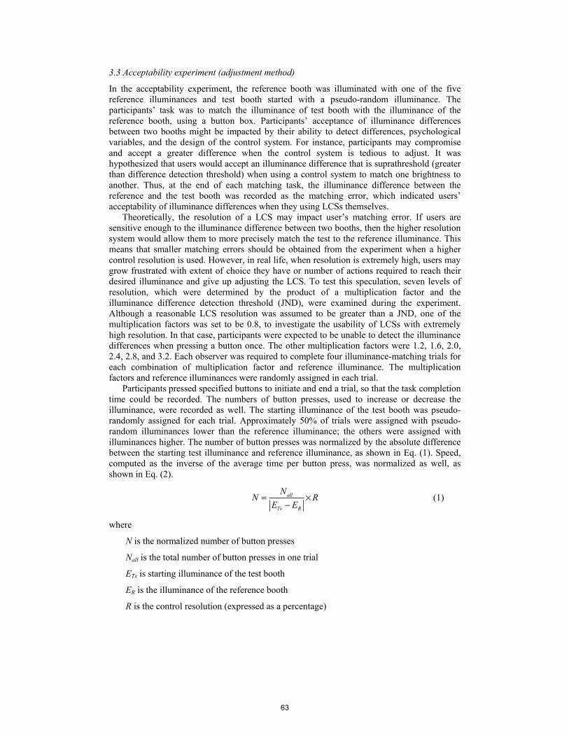
3.3 Acceptability experiment (adjustment method)

In the acceptability experiment, the reference booth was illuminated with one of the five reference illuminances and test booth started with a pseudo-random illuminance. The participants’ task was to match the illuminance of test booth with the illuminance of the reference booth, using a button box. Participants’ acceptance of illuminance differences between two booths might be impacted by their ability to detect differences, psychological variables, and the design of the control system. For instance, participants may compromise and accept a greater difference when the control system is tedious to adjust. It was hypothesized that users would accept an illuminance difference that is suprathreshold (greater than difference detection threshold) when using a control system to match one brightness to another. Thus, at the end of each matching task, the illuminance difference between the reference and the test booth was recorded as the matching error, which indicated users’ acceptability of illuminance differences when they using LCSs themselves.

Theoretically, the resolution of a LCS may impact user’s matching error. If users are sensitive enough to the illuminance difference between two booths, then the higher resolution system would allow them to more precisely match the test to the reference illuminance. This means that smaller matching errors should be obtained from the experiment when a higher control resolution is used. However, in real life, when resolution is extremely high, users may grow frustrated with extent of choice they have or number of actions required to reach their desired illuminance and give up adjusting the LCS. To test this speculation, seven levels of resolution, which were determined by the product of a multiplication factor and the illuminance difference detection threshold (JND), were examined during the experiment. Although a reasonable LCS resolution was assumed to be greater than a JND, one of the multiplication factors was set to be 0.8, to investigate the usability of LCSs with extremely high resolution. In that case, participants were expected to be unable to detect the illuminance differences when pressing a button once. The other multiplication factors were 1.2, 1.6, 2.0, 2.4, 2.8, and 3.2. Each observer was required to complete four illuminance-matching trials for each combination of multiplication factor and reference illuminance. The multiplication factors and reference illuminances were randomly assigned in each trial.

Participants pressed specified buttons to initiate and end a trial, so that the task completion time could be recorded. The numbers of button presses, used to increase or decrease the illuminance, were recorded as well. The starting illuminance of the test booth was pseudo-randomly assigned for each trial. Approximately 50% of trials were assigned with pseudo-random illuminances lower than the reference illuminance; the others were assigned with illuminances higher. The number of button presses was normalized by the absolute difference between the starting test illuminance and reference illuminance, as shown in Eq. (1). Speed, computed as the inverse of the average time per button press, was normalized as well, as shown in Eq. (2).

all

Ts R

NN R

E E= ×

− (1)

where

N is the normalized number of button presses

Nall is the total number of button presses in one trial

ETs is starting illuminance of the test booth

ER is the illuminance of the reference booth

R is the control resolution (expressed as a percentage)

63

all

Ts R

NS

CT

E E

=

−

(2)

where

S is the normalized speed of button presses. It is the inverse of the average time consumed between two button presses

Nall is the total number of button presses in one trial

ETs is starting illuminance of the test booth

ER is the illuminance of the reference booth

CT is the completion time for each trial After completing all experimental trials for one LCS resolution, each participant was

instructed to complete an after-scenario questionnaire (ASQ), as shown in Table 1.

Table 1. The After-Scenario Questionnaire (ASQ).

Strongly disagree

Strongly

agree I am confident with the accuracy of my matches.

1 2 3 4 5 6 7

I am satisfied with the speed with which I was able to make matches with this control system.

1 2 3 4 5 6 7

Overall, I am satisfied with the ease of making the matches with this control system.

1 2 3 4 5 6 7

3.4 Proposed step-dimming curves

Based on the results from the detectability and acceptability experiments, a series of step-dimming curves were developed for LCSs of various resolutions. Simulated illuminance was initially set to the maximum (drive current of 1.0 A for the LED light engines considered) in MatLab and illuminance was gradually reduced, in steps dictated by the control resolution. According to the Weber’s Law, the perception of a just noticeable difference in illuminance is proportional to the mean illuminance. Therefore, the change in illuminance between two dimming steps was the resolution multiplied by the illuminance. These calculations were repeated until the current reached 1% of the maximum (0.01 A). Normalized illuminance, which is the percentage of the maximum illuminance, was plotted for each step. Power consumption as a function of dimmer setting was measured during these iterative calculations.

The resultant dimming curve was compared to common continuous dimming curves used in commercially available lighting products. MatLab was used to generate the proposed step-dimming curve first and then to compare the proposed curve to continuous dimming curves. The two most popular dimming curves, a logarithmic dimming curve and a Square Law curve, were compared with the proposed function. As manufacturers do not provide equations for their continuous logarithmic curves, in this project, the continuous logarithmic curve was mathematically expressed by the equation corresponding to the base function of the proposed step-dimming curve. As this type of function is commonly referred as a “logarithmic dimming curve” in the lighting industry, that term is used here. The Square Law curve is reported to be generally rated favorably by end users [15, 16]. Both the logarithmic and Square Law curves are commonly used in products from lighting control manufacturers, such as Lutron and Dynalite [4, 17].

64

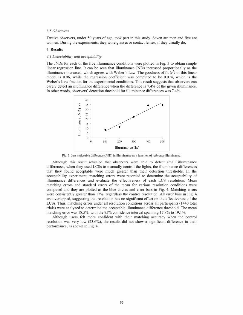
3.5 Observers

Twelve observers, under 50 years of age, took part in this study. Seven are men and five are women. During the experiments, they wore glasses or contact lenses, if they usually do.

4. Results

4.1 Detectability and acceptability

The JNDs for each of the five illuminance conditions were plotted in Fig. 3 to obtain simple linear regression line. It can be seen that illuminance JNDs increased proportionally as the illuminance increased, which agrees with Weber’s Law. The goodness of fit (r2) of this linear model is 0.96, while the regression coefficient was computed to be 0.074, which is the Weber’s Law fraction for the experimental conditions. This result suggests that observers can barely detect an illuminance difference when the difference is 7.4% of the given illuminance. In other words, observers’ detection threshold for illuminance differences was 7.4%.

Fig. 3. Just noticeable difference (JND) in illuminance as a function of reference illuminance.

Although this result revealed that observers were able to detect small illuminance differences, when they used LCSs to manually control the lights, the illuminance differences that they found acceptable were much greater than their detection thresholds. In the acceptability experiment, matching errors were recorded to determine the acceptability of illuminance differences and evaluate the effectiveness of each LCS resolution. Mean matching errors and standard errors of the mean for various resolution conditions were computed and they are plotted as the blue circles and error bars in Fig. 4. Matching errors were consistently greater than 17%, regardless the control resolution. All error bars in Fig. 4 are overlapped, suggesting that resolution has no significant effect on the effectiveness of the LCSs. Thus, matching errors under all resolution conditions across all participants (1440 total trials) were analyzed to determine the acceptable illuminance difference threshold. The mean matching error was 18.5%, with the 95% confidence interval spanning 17.8% to 19.1%.

Although users felt more confident with their matching accuracy when the control resolution was very low (23.6%), the results did not show a significant difference in their performance, as shown in Fig. 4.

65

Fig. 4. Matching errors and users’ confidence in matching accuracy as a function of LCS resolution. Mean matching errors and standard error of the mean (SEM) are shown as the blue circles and error bars (left y-axis). Users’ median subjective ratings of their confidence with their matching accuracy are shown by red triangles (right y-axis).

The normalized numbers of button presses per trial, obtained from Eq. (1), and the mean speed per button press, obtained from Eq. (2), were calculated to assess efficacy with which the LCS enable the users to reach their desired illuminance. The normalized number of button presses as a function of the resolution are shown in Fig. 5. Theoretically, if the resolution has no effect on users’ behavior, these numbers of button presses with various resolution systems should be the same or very similar. It can be seen in Fig. 5 that, when the resolution is extremely low (23.6% or 20.7%), the normalized number of button presses is significantly greater than with other resolutions. Those extra presses suggest that participants did not accept the relatively large illuminance differences induced, and tried to adjust the illuminance by repeatedly pressing the upward and downward buttons. This was observed by the experimenter and also reported by some participants.

Fig. 5. The effect of control resolution on the normalized number of button presses. Error bars show standard error of the mean (SEM).

The mean speed per button press was calculated as the inverse of the average time consumed between two button presses. As shown in Fig. 6, mean speed per button press

66

decreases as the resolution increases. When the LCS resolution is very high (values lower than 14.8%), the normalized speed per button press is significantly slower than with LCSs of lower resolutions. During the experiment, all participants reported that the extremely high resolution (5.9%) condition made them confused and that they spent more time checking whether the LCS was working properly.

Fig. 6. Mean normalized speed per button press and subjective ratings. The left y-axis shows the mean speed and the right y-axis shows the scale of the subjective ratings. The “+” markers show the median ratings of users’ confidence with matching accuracy. The “X” markers show the median ratings of users’ satisfaction with their matching speed. The solid circles show the median ratings of users’ overall satisfaction. Error bars show standard error of the mean (SEM).

Participants’ subjective ratings are also shown in Fig. 6, to compare with the psychophysical data. As shown in Fig. 6, the decreased speed with higher resolution LCSs is consistent with decreased user satisfaction with the speed, as well as overall satisfaction. It may suggest that satisfaction relates to the speed with which users can reach their desired illuminance, rather than the accuracy with which they can achieve their desired illuminance.

To conclude, users are able to detect illuminance differences of 7.4% of the initial illuminance and they accept illuminance differences of 17.9% to 19.1%. When matching errors, normalized numbers of button presses, mean speed per button press and users’ subjective ratings are collectively considered, the results suggest that the most efficient and user-friendly manual lighting control systems are those with resolutions ranging from 14.8% and 17.7%.

4.2 Dimming curves

A series of step-dimming curves were developed with resolutions ranging from 7% (within detectability limits) to 17% (within acceptability limits). The total number of dimming steps varied as the resolutions varied. For example, there were 65 steps to dim from 100% to 1% with a resolution of 7%, but only 26 steps when the resolution was 17%. To compare the different dimming curves on the same scale, the number of dimming steps was normalized to 100 and power consumption was normalized as a percentage of the maximum power. In Fig. 7-9, the gray bars show the difference in normalized power between the two dimming curves at each setting. The actual amount of energy conserved would depend on the frequency of each setting’s use, which would depend on the application, user behavior, etc. The average was obtained by simply assuming that each setting is equally likely to be used. This method probably underestimates the average energy savings for real applications, since higher settings may be used more frequently than lower settings.

67

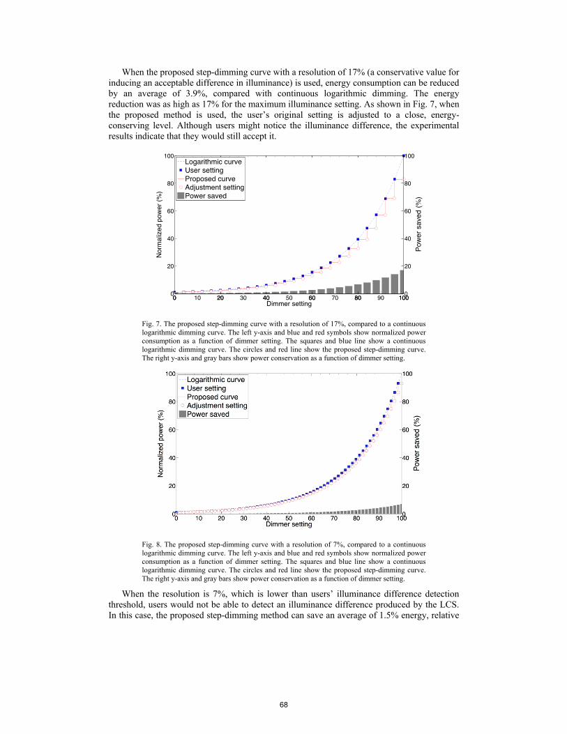
When the proposed step-dimming curve with a resolution of 17% (a conservative value for inducing an acceptable difference in illuminance) is used, energy consumption can be reduced by an average of 3.9%, compared with continuous logarithmic dimming. The energy reduction was as high as 17% for the maximum illuminance setting. As shown in Fig. 7, when the proposed method is used, the user’s original setting is adjusted to a close, energy-conserving level. Although users might notice the illuminance difference, the experimental results indicate that they would still accept it.

Fig. 7. The proposed step-dimming curve with a resolution of 17%, compared to a continuous logarithmic dimming curve. The left y-axis and blue and red symbols show normalized power consumption as a function of dimmer setting. The squares and blue line show a continuous logarithmic dimming curve. The circles and red line show the proposed step-dimming curve. The right y-axis and gray bars show power conservation as a function of dimmer setting.

Fig. 8. The proposed step-dimming curve with a resolution of 7%, compared to a continuous logarithmic dimming curve. The left y-axis and blue and red symbols show normalized power consumption as a function of dimmer setting. The squares and blue line show a continuous logarithmic dimming curve. The circles and red line show the proposed step-dimming curve. The right y-axis and gray bars show power conservation as a function of dimmer setting.

When the resolution is 7%, which is lower than users’ illuminance difference detection threshold, users would not be able to detect an illuminance difference produced by the LCS. In this case, the proposed step-dimming method can save an average of 1.5% energy, relative

68

to continuous logarithmic dimming, as shown in Fig. 8. Although the energy savings are fairly small when with this LCS resolution is compared to a continuous logarithmic dimming method, the change in illumination would be undetectable by users.

The proposed dimming curves are designed based on a basic logarithmic dimming curve, which is believed to be sensible, since it can be deduced from the Weber’s law. Thus, the energy conservation compared to logarithmic dimming curve is less than the energy savings when compared to other dimming curves. When this method is compared to a Square Law dimming curve, the amount of conserved power increases substantially. Figure 9 shows power consumption and power conservation when the proposed method is compared to a Square Law dimming curve. Table 2 summarizes comparisons with both dimming curves.

Fig. 9. The proposed step-dimming curve with a resolution of 17%, compared to a continuous Square Law dimming curve. The left y-axis and blue and red symbols show normalized power consumption as a function of dimmer setting. The squares and blue line show a continuous Square Law dimming curve. The circles and red line show the proposed step-dimming curve. The right y-axis and gray bars show power conservation as a function of dimmer setting.

Table 2. Energy Saved when the Proposed Step-Dimming Curve is Used, Relative to Continuous Dimming Curves

Resolution (%)

Energy conservation (%) Relative to continuous logarithmic

dimming Relative to continuous Square Law

dimming Average Maximum Average Maximum

17.0 3.85 17.0 15.4 31.3 15.0 3.33 15.0 15.2 30.8 7.00 1.54 7.00 13.4 27.4

5. Discussion

From results of psychophysical experiments, which indicate that illuminance differences of about 7.4% are barely detectable, and differences from 17.8% to 19.1% are acceptable, implementation of the step-dimming curve proposed here should generally have a resolution from 7.4% to 19.1%. The study of the usability of LCSs with various resolutions shows that a resolutions from 14.8% and 17.7% are most suitable for manual LCSs.

With a 17% difference in illuminance, users will be capable of detecting the difference between their desired illuminance and the illuminance that they are able to achieve, but will still find it acceptable. This could be useful for lighting applications that are not primarily driven by the performance of critical visual tasks, such as hotels, restaurants, and some residential spaces. If lighting control systems were to use the proposed step-dimming curve with a resolution between 14.8% and 17.7%, energy consumption would be reduced, LED

69

luminous efficacy would be increased, and the user experience of the LCSs would be improved. When using the proposed curve with a resolution of 7%, users would not be able to detect illuminance differences. However, the high resolution could potentially lead to user dissatisfaction with manual control systems. Until further research investigates user acceptance of the proposed method with very high resolutions, it might be considered primarily for automatic control systems, such as daylight harvesting systems.

In the acceptability experiment, participants performed matching tasks with two side-by-side booths—simultaneous stimuli were compared. However, in real lighting applications, users typically compare the illuminance before and after their adjustment of the control system, and the two illuminances are not simultaneously compared. Furthermore, in many situations, users compare the achieved illuminances with a desired illuminance that exists only in their imagination. Therefore, the data from the simultaneous comparison in this project presents the “worst-case scenario” and the difference detection thresholds and acceptance thresholds obtained are likely smaller than they would be in a real world applications.

Akashi reported that observers’ memory for illuminance fades and sensitivity to illuminance differences decreases more after 100 seconds than after three seconds [1]. Therefore, continuous dimming curves could be used when occupants actively control the lights. Then, after a setting is made, the illuminance could be adjusted to the closest level in the proposed curve after a delay, such as 100 seconds.

Furthermore, it is noteworthy that energy consumption can be reduced with dimming, not only by reducing unnecessary illuminance, but also by driving LEDs at higher efficacies. The efficacy droop measured and used in the calculations reported here were lower in magnitude than many commercialized products. The LED light engines in this project were directly attached to large, high-quality heat sinks, and were located in a well-ventilated space. Commercialized products in enclosed luminaires and mounted in tight spaces will be more significantly impacted by thermal droop [18]. Thus, with the proposed dimming method, higher energy savings would be expected in real-world applications than the laboratory results reported here.

These experiments were conducted under laboratory conditions, which involved two illuminated booths in a windowless dark room. The results may differ in the real lighting applications since the experimental environment differed from typical illuminated environment. This research aims to provide a generalized understanding to guide the design of control systems and initiate rigorous consideration of control resolutions. The proposed dimming curves are derived from experimental results, but still theoretical in nature. Should manufacturers adopt them for use in their products, adjustments will likely need to be made to suit the design and intended function of the lighting systems. Field studies could be conducted in the future to examine the applicability of the findings of this project to real architectural environments.

6. Conclusion

The first experiment found that horizontal illuminance differences of approximately 7.4% were able to be detected by participants in controlled laboratory conditions. Surprisingly, in those same conditions, participants found matching errors of 17.8% to 19.1% to be acceptable in the second experiment. This suggests that users are capable of detecting small illuminance differences, but have a considerably higher illuminance difference acceptance threshold when given control of the lighting system. A theoretical step dimming method was proposed to conserve energy. Field studies could be conducted to validate and refine the proposed method for use in commercial products.

70

Chapter 4. Luminance resolution of lighting control systems:

usability and energy conservation

71

LUMINANCE RESOLUTION OF LIGHTING CONTROL SYSTEMS: USABILITY AND ENERGY CONSERVATION

Hu, W.1, Davis, W.2 1,2 Faculty of Architecture, Design and Planning, The University of Sydney, NSW 2006,

AUSTRALIA 1wehu7684@uni.sydney.edu.au

Abstract

Following on from studies of illuminance resolution, experiments have been conducted to investigate the impact of luminance resolution on the usability of lighting control systems (HU & DAVIS, 2015). Users’ ability to detect luminance differences on luminaire surfaces is found to be 10,5 % to 13,5 %, which shows less sensitivity to luminance differences than illuminance differences on surfaces, for values of these quantities that are representative of typical architectural lighting conditions. When users look at luminaires directly to adjust them, control systems with resolutions from 26,0 % to 32,5 % have better usability than those with other resolutions. Thus, a new step-dimming curve is proposed, so that energy consumption could be reduced by an average of 7,7 % compared to a continuous logarithmic dimming system, and by 18,9 % compared to a square law dimming curve system.

Keywords: lighting control systems, usability, dimming curve, energy conservation, illumination design

1 Background

A number of studies have investigated brightness discrimination, which describes the just noticeable difference, or discrimination threshold (∆L), between a stimulus of a given luminance and its background luminance (BARLOW, 1957; NORTON & CORLISS, 2002). Older investigations measured the relationship between the intensities of stimuli and visual perception, to better understand the human visual system. Most of the experimental stimuli were of relatively low luminance—typically less than 1000 cd/m2. In the real world, occupants operate lighting control systems (LCSs) in bright environments and the luminance of typical lamp or luminaire surfaces is significantly greater than 1000 cd/m2.

Furthermore, an increasing number of commercial lighting control products are designed with high resolution, referring to the smallest brightness change that can be produced by a LCS. Previous research studied the relationship between illuminance resolution and usability (HU & DAVIS, 2015). This study further investigates the impact of luminance resolution, because users sometimes make their LCS settings while looking directly at the luminaires being adjusted. If the impact of LCS resolution on user perception and behaviour is understood, small adjustments can be made to the lighting to reduce energy consumption, without negatively impacting the visual appearance of the illuminated environment. This research combines psychophysical methods and questionnaires to investigate the impact of LCS luminance resolution on users’ visual perception and satisfaction. These findings can be applied to develop LCSs that reduce the energy consumed by lighting.

2 Methods

In the Lighting Lab at the University of Sydney, two identical side-by-side light booths were constructed, as shown in Figure 1. A micro-lens diffuser, with a diameter of 12 cm, was recessed on the back wall of each booth. The observers’ viewing distance to the diffusers was 2,7 m, so that the diffuser subtended a visual angle that was similar to the visual angle of an MR16 downlight seen by a seated person in a typical architectural space. LED light engines were mounted behind the two diffusers and the luminance of the front face of each diffuser was measured under five drive current conditions: 0,1 A, 0,3 A, 0,5 A, 0,7 A, and 0,9 A. This

72

data was used to derive an equation describing the relationship between luminance and current.

(a) (b)

Figure 1 – (a) Experimental setup. Overhead lights were only on to capture photograph. (b) Section view of the experimental setup.

2.1 Preliminary experiments A two-alternative-forced-choice (2AFC) experiment was initially used to measure the just noticeable difference (JND) in luminance. In this experiment, the two diffusers in the booths were randomly assigned with the reference and test luminance. Observers were instructed to identify the brighter diffuser. Based on luminance measurements of real lighting installations, the reference luminances were 1000 cd/m2, 2000 cd/m2, 3000 cd/m2, or 4000 cd/m2, while the test luminances were 8 %, 16 %, 24 %, 32 % or 40 % lower than the reference luminance. Each observer completed 10 trials for each combination of reference and test luminance, in a random sequence. When observers were able to correctly identify the higher luminance source on 75 % of trials, the difference between the reference and test luminance was determined as the just noticeable difference (JND) for that reference luminance. A percentage was calculated from the ratio of the JND to the reference luminance, indicating the detection threshold of luminance differences when users looked directly at the light to adjust it.

However, a follow-up preliminary experiment found that, when adjusting a single luminous diffuser, users were able to detect luminance differences smaller than the detection thresholds obtained in the first experiment. This is likely because the initial JND was obtained when the two diffusers were presented side-by-side. However, in the second preliminary experiment, as well as in real life situations, the luminance of a luminaire before and after users adjusting would be compared. Thus, another experiment was conducted with only a single diffuser and participants were instructed to compare the diffuser’s luminance before and after making their adjustments. Nevertheless, this experiment failed to yield meaningful data, since participants’ were visually adapting throughout the experiment. All participants reported that luminance changed even when the current driving the LED light engines did not change. This failure suggested that it might be impractical to study detection thresholds of temporally changing stimuli of high intensities. Thus, another psychophysical method – the method of adjustment– was used to examine the detection thresholds again, based on the original side-by-side experimental setup.

The experimental setup of the adjustment experiment was the same with the 2AFC experiment. In this experiment, the reference diffuser had luminances of 1000 cd/m2, 2000 cd/m2, 3000 cd/m2, 4000 cd/m2 or 5000 cd/m2, randomly presented. Participants adjusted the luminance of the test diffuser by using a control box to match the reference luminance. The resolution of this control system was set to be extremely high (0,5 %) to ensure that it did not

73

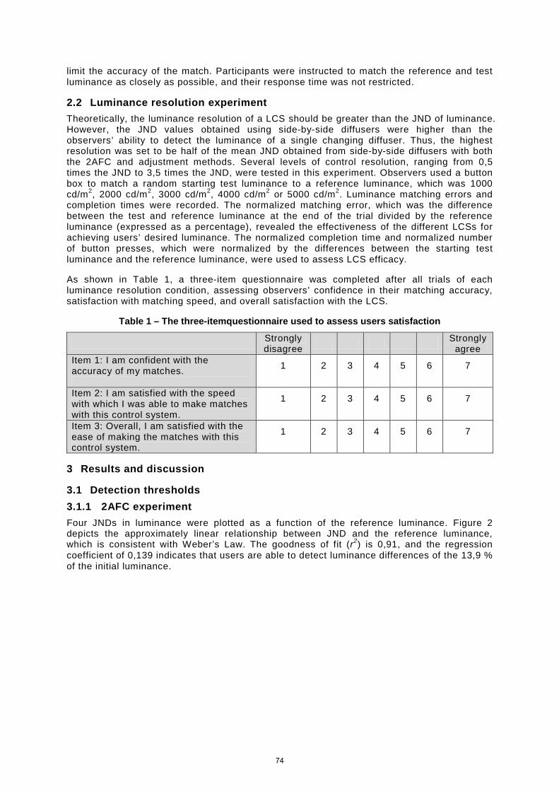
limit the accuracy of the match. Participants were instructed to match the reference and test luminance as closely as possible, and their response time was not restricted.

2.2 Luminance resolution experiment Theoretically, the luminance resolution of a LCS should be greater than the JND of luminance. However, the JND values obtained using side-by-side diffusers were higher than the observers’ ability to detect the luminance of a single changing diffuser. Thus, the highest resolution was set to be half of the mean JND obtained from side-by-side diffusers with both the 2AFC and adjustment methods. Several levels of control resolution, ranging from 0,5 times the JND to 3,5 times the JND, were tested in this experiment. Observers used a button box to match a random starting test luminance to a reference luminance, which was 1000 cd/m2, 2000 cd/m2, 3000 cd/m2, 4000 cd/m2 or 5000 cd/m2. Luminance matching errors and completion times were recorded. The normalized matching error, which was the difference between the test and reference luminance at the end of the trial divided by the reference luminance (expressed as a percentage), revealed the effectiveness of the different LCSs for achieving users’ desired luminance. The normalized completion time and normalized number of button presses, which were normalized by the differences between the starting test luminance and the reference luminance, were used to assess LCS efficacy.

As shown in Table 1, a three-item questionnaire was completed after all trials of each luminance resolution condition, assessing observers’ confidence in their matching accuracy, satisfaction with matching speed, and overall satisfaction with the LCS.

Table 1 – The three-itemquestionnaire used to assess users satisfaction

Strongly disagree Strongly

agree Item 1: I am confident with the accuracy of my matches.

1 2 3 4 5 6 7

Item 2: I am satisfied with the speed with which I was able to make matches with this control system.

1 2 3 4 5 6 7

Item 3: Overall, I am satisfied with the ease of making the matches with this control system.

1 2 3 4 5 6 7

3 Results and discussion

3.1 Detection thresholds 3.1.1 2AFC experiment Four JNDs in luminance were plotted as a function of the reference luminance. Figure 2 depicts the approximately linear relationship between JND and the reference luminance, which is consistent with Weber’s Law. The goodness of fit (r2) is 0,91, and the regression coefficient of 0,139 indicates that users are able to detect luminance differences of the 13,9 % of the initial luminance.

74

Figure 2 – Just noticeable difference(JND) as a function of reference luminance for the 2AFC experiment.

3.1.2 Adjustment experiment In the adjustment experiment, detection threshold was estimated as the ratio of matching error to the reference luminance. Technically, this represents the maximum change in luminance that observers are unable to detect, rather than just barely detect (JND). However, this value is expected to be very close to the JND. Detection thresholds, measured from five participants, are shown in Figure 3. The circles show the mean matching error (as a percentage of reference luminance) of each participant, and the error bars show the bootstrap confidence intervals. Bootstrapping, which is a method based on a large number of calculations, is a well-accepted technique to estimate the unknown parameter of the whole population (EFRON & TIBSHIRANI, 1986). In this experiment, 5000 bootstrap replications were calculated in MatLab.

Figure 3 – Detection thresholds for luminance differencesforfive subjects. Error bars show bootstrap confidence intervals.

The distribution of data from the entire 360 trials is shown in Figure 4. The median is 12,0 %and the 95 % confidence interval is +/- 1,5 %. The detection thresholds under this experimental condition ranges from 10,5 % to 13,5 %, which suggests detection thresholds for the entire population could be estimated to fall within this range. This result is consistent with the result obtained from the 2AFC experiment.

75

Figure 4 – The probability distribution of the matching errors (percentage of reference luminance) across all participants.

It is can be seen that, in this side-by-side experimental setting, the detection thresholds obtained from two different designed experiments are close. Ultimately, the luminance difference detection threshold was estimated as the mean of results obtained from two experiments, which was calculated to be 13,0 %. This result, based on two different methods, a large amount of data and statistical analysis, could be used as the theoretical threshold for noticeable luminance difference.

Previous research, using a similar side-by-side experimental setting, has found that users are able to perceive differences of 7,4 % in illuminance (Hu & Davis, 2015), for illuminances that are common in architectural spaces. The difference between the illuminance JND and luminance JND suggests that users’ ability to detect illuminance differences on surfaces is more sensitive than their ability to detect luminance differences on luminaire surfaces, for the values of these quantities tested. This is not surprising—the surfaces of luminaires have very high luminances, whereas illuminated spaces are significantly less bright.

As mentioned in section 2.1, the measurement of detection thresholds of luminance differences in real life conditions is impractical due to ongoing visual adaptation. Nonetheless, a few of the conditions in a preliminary experiment, using a single light system with a resolution of 0,5, 0,6, 0,7 or 0,8 times of the mean detection threshold from the two experiments, was examined. When resolution was 6,5 %, which is half of detection threshold, all participants reported that the change in luminance caused by a single button press could not be perceived. All observers reported a perceived change when the resolution was 10,4 % (0,8 times detection threshold). Resolutions of 7,8 % and 9,1 % did not receive consistent judgements across all participants. It suggested that the detection thresholds in real life scenarios might fall within this range.

3.2 Usability of LCSs with various resolutions 3.2.1 Effectiveness The effectiveness of the LCSs with various resolutions was assessed by the normalized matching errors, which is explained in section 2.3. Figure 5 shows matching error as a function of resolution. There is no significant difference in matching error when the resolution is between 6,5 % and 26 %. Although the error bars of the 45,5 % resolution overlap with the error bars of 13 % and 26 % resolutions, they do not overlap with the 6,5 % and 19,5 % resolutions. When the resolution is 45,5 %, the matching error will necessarily be very high because each button press changes the luminance by 45,5 %. The percentage matching errors are significantly higher when the resolution is 32,5 - 39 % than the higher control resolutions tested.

76

Figure 5 – Matching error as a function of control resolution. Error bars show 95 % confidence intervals.

3.2.2 Efficacy Task completion time and speed are usually used to evaluate the efficacy of a control system. In this experiment, task completion time was normalized by the starting difference between the reference and test luminance. As shown in Figure 6, LCSs with resolutions of 6,5 % and 45,5 % are much more time-consuming than the others. When the resolution is 13 %, users spend more time to make a match than with a 39 % resolution system. For resolutions ranging from 19,5 % to 32,5 %, no significant effect of resolution can be established on the amount of time consumed to make match settings.

Figure 6 – Normalized matching time as a function of resolution. Error bars show 95 % confidence intervals.

The normalized number of button presses is another criterion to assess the efficacy of LCSs. When using LCSs with inefficient resolutions, participants may excessively press the buttons. High resolution inherently leads to more button presses, thus the number of button presses was normalized, not only by the starting luminance differences, but also by the resolution itself. Theoretically, if resolution has no effect on the LCSs’ efficacy, the normalized number of button presses would be the same or at least similar for all resolutions. Conversely, as

77

shown in Figure 7, the resolutions of 32,5 % and 45,5 % lead to more button presses than the other resolutions.

Figure 7 – Normalized number of button presses as a function of resolution. Error bars show 95 % confidence intervals.

The normalized speed per button press was determined by the normalized time divided by the normalized number of button presses. It measures the speed of each button press, instead of the speed of completing the entire task. The latter would be the inverse of the total completion time. As shown in Figure 7 and Figure 8, users pressed the buttons most with a resolution of 32,5 %, but the mean speed of each button press was much faster than with the other resolutions, suggesting that they spent less time thinking or viewing. All participants reported, during the experiment, that extremely high resolutions (e.g. 6,5 %) made them confused and they spent more time checking whether the LCS worked properly. When the resolution reduces from 6,5 % to 32,5 %, the normalized speed per button press increases considerably and drops when resolution is lower than 32,5 %, as shown in Figure 8. When resolution was extremely low (more than 39 %), participants mentioned that the difference between reference and test luminance were not acceptable. They spent more time comparing the luminance changes caused by one button press when the test luminance was approaching the reference luminance.

78

Figure 8 – Normalized speed per button press as a function of resolution. Error bars show 95 % confidence intervals.

3.3 User satisfaction The median (Mdn) and interquartile range (IQR) of subjective ratings of each resolution condition were calculated, as shown in Table 2.

Table 2 – The median (Mdn) and interquartile range (IQR) of subjective ratings.

Resolution 6,5% 13,0% 19,5% 26,0% 32,5% 39,0% 45,5%

Item 1 Mdn 4,0 5,0 5,0 5,0 6,0 5,0 5,0 IQR 1,8 1,0 1,0 0,8 1,0 1,8 1,0

Item 2 Mdn 3,0 4,0 5,0 5,0 6,0 6,0 5,5 IQR 2,0 3,0 5,0 4,3 5,0 5,0 5,0

Item 3 Mdn 4,0 4,5 5,0 5,0 6,0 6,0 6,0 IQR 2,0 2,0 1,0 1,8 1,0 1,0 1,8

The frequency distributions of responses from Likert scales questionnaires were shown in Figure 9. Users felt most confident of their matching accuracy with the 32,5 % resolution (Mdn=6, IQR=1,0) and least confident with the highest resolution (6,5 %) condition (Mdn=4, IQR=1,8). There were no significant differences in confidence with the other resolutions. Users’ satisfaction with speed increased with the decrease of resolution until the resolution became extremely low (45,5 %), as shown in Figure 9 (b). Most respondents indicated that overall satisfaction with lower resolution systems (resolutions between 32,5 % to 39,0 %) was greater (Mdn=6, IQR=1,0) than with the higher resolution systems.

79

Figure 9 – Frequency distributions of questionnaire responses. The central rectangles span the interquartile ranges (top edges show the third quartile and the bottom edges show the first

quartile). Red lines show the median and the whiskers above and below the rectangle show the maximum and minimum, respectively.

3.4 Energy conservation The combined results of the psychophysical experiment and users’ subjective ratings indicate that the usability of LCSs with the resolutions from 26,0 % to 32,5 % is greater than with the other resolutions, when users look at the lights directly to adjust brightness. A mathematical model and step-dimming curves were proposed to conserve energy by reducing the illuminance, in a manner that is either unnoticeable or noticeable, but still acceptable (HU & DAVIS, 2015). The same method was used in the project. A step-dimming curve with a resolution of 32,5 %, as shown in Figure 10, can be used in a manual dimming system. Lighting control systems with this proposed step-dimming curve consume 7,7 % (on average) less energy than systems with traditional logarithmic dimming curves and 18,9 % less than those with square law dimming curves, as shown in Figure 11.

80

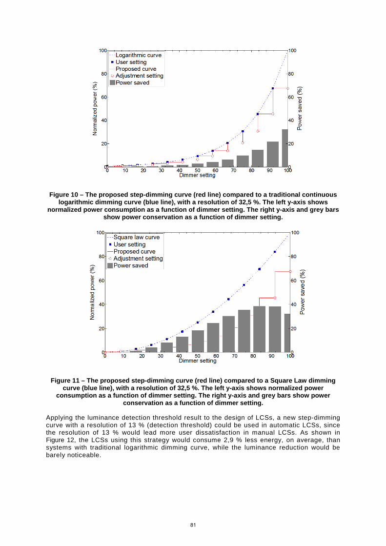
Figure 10 – The proposed step-dimming curve (red line) compared to a traditional continuous logarithmic dimming curve (blue line), with a resolution of 32,5 %. The left y-axis shows

normalized power consumption as a function of dimmer setting. The right y-axis and grey bars show power conservation as a function of dimmer setting.

Figure 11 – The proposed step-dimming curve (red line) compared to a Square Law dimming curve (blue line), with a resolution of 32,5 %. The left y-axis shows normalized power

consumption as a function of dimmer setting. The right y-axis and grey bars show power conservation as a function of dimmer setting.

Applying the luminance detection threshold result to the design of LCSs, a new step-dimming curve with a resolution of 13 % (detection threshold) could be used in automatic LCSs, since the resolution of 13 % would lead more user dissatisfaction in manual LCSs. As shown in Figure 12, the LCSs using this strategy would consume 2,9 % less energy, on average, than systems with traditional logarithmic dimming curve, while the luminance reduction would be barely noticeable.

81

Figure 12 – The proposed step-dimming curve (red line) compared to a traditional continuous logarithmic dimming curve (blue line), with a resolution of 13 %.The left y-axis shows

normalized power consumption as a function of dimmer setting. The right y-axis and grey bars show power conservation as a function of dimmer setting.

4 Conclusions

The usability of LCSs with various luminance resolutions was assessed. Extremely high resolution (6,5 %), which simulated a so-called “seamless” dimming system in the market, led to increased user dissatisfaction, while extremely low resolutions, such as 39,0 %, caused more setting errors.

Energy reduction simulations were performed on the middle-range resolutions, which resulted in the highest user efficacy, efficiency, and satisfaction. For a given user luminance setting, the simulated system automatically reduced luminance to a slightly lower level, resulting in a barely perceptible, but likely acceptable, difference in luminance. Compared to a continuous logarithmic dimming system, which has an extremely high resolution, LCSs with a resolution of 32,5 % could reduce energy consumption by an average of 7,7 %, when this strategy is used. This finding may be able to be leveraged in the design of interactive lighting systems that maintain the visual appearance of the environment and reduce energy consumption.

References

BARLOW, H., 1957. Increment thresholds at low intensities considered as signal/noise discriminations. The Journal of Physiology 136.3, pp. 469-488.

EFRON, B. & TIBSHIRANI, R., 1986. Bootstrap Methods for Standard Errors, Confidence Intervals, and Other Measures of Statistical Accuracy. Statistical Science, 1(1), p. 54–75.

HU, W. & DAVIS, W., 2015. Dimming Curve Based on the Detectability and Acceptability of Illuminance Differences. Suzhou, China, OSA, Light Energy and the Environment Congress.

HU, W. & DAVIS, W., 2015. Illuminance resolution and usability of interactive lighting control systems. Manchester, United Kingdom, CIE, pp. 469-479.

NORTON, T. T. & CORLISS, D. A., 2002. The psychophysical measurement of visual function. s.l.:Butterworth-Heinemann.

82

Chapter 5. Development and Evaluation of Colour Control

Interfaces for LED Lighting

83

Development and evaluation of colour control interfaces for LED lighting WENYE HU* AND WENDY DAVIS Faculty of Architecture, Design and Planning, The University of Sydney, NSW 2006, Australia *wehu7684@uni.sydney.edu.au

Abstract: To capitalise on the colour tuning capabilities of LED lighting, a model for converting device-specific control signals to chromaticity coordinates was used in a psychophysical experiment evaluating the usability of three colour control interfaces based on RGB (red, green, blue), HSB (hue, saturation, brightness) and opponent colour mixing systems. Although common and well accepted, the RGB interface had lowest usability based on both psychophysical results and subjective ratings. The usability of HSB and opponent colour interfaces was not significantly different. These findings can guide the development of useful and efficient colour control interfaces for tunable LED lighting systems. © 2017 Optical Society of America

OCIS codes: (330.1730) Colorimetry; (330.5510) Psychophysics; (350.4600) Optical engineering.

References and links 1. S. O. Marberry and L. Zagon, The Power of Color: Creating Healthy Interior Spaces (Wiley, 1995). 2. F. Viénot, G. Coron, and B. Lavédrine, “LEDs as a tool to enhance faded colours of museums artefacts,” J. Cult.

Herit. 12(4), 431–440 (2011). 3. D. Abdalla, A. Duis, D. Durmus, and W. Davis, “Customization of light source spectrum to minimize light

absorbed by artwork,” in Proceedings of CIE Lighting Quality and Energy Efficiency Conference 2016 (Commission Internationale de L'Eclairage, 2016), pp. 22–31.

4. M. Wood, “Many shades of white,” Stage Directions 23 (9), (2010). 5. T. A. LeGates, D. C. Fernandez, and S. Hattar, “Light as a central modulator of circadian rhythms, sleep and

affect,” Nat. Rev. Neurosci. 15(7), 443–454 (2014). 6. W. Julian, “The Sydney opera house concert hall celebrates two years of LEDs,” Lighting 36(4), 26–27 (2016). 7. A. R. Smith, “Colour gamut transform pairs,” Comput Graph (ACM). SIGGRAPH 12(3), 12–19 (1978). 8. M. W. Schwarz, W. B. Cowan, and J. C. Beatty, “An experimental comparison of RGB, YIQ, LAB, HSV, and

opponent color models,” ACM Trans. Graph. 6(2), 123–158 (1987). 9. S. Beigpour and M. Pedersen, “Color Play: Gamification for Color Vision Study,” in Proceedings of Color and

Image, Midterm Meeting of the International Colour Association (AIC, 2015). 10. J. Schanda, Colorimetry: Understanding the CIE System (John Wiley & Sons, Inc., 2007). 11. C. V. R. Labs, Colour and Vision Database: Colour Matching Functions. Available: http://www.cvrl.org/ (2016) 12. D. B. Judd, Colorimetry (U.S. Govt Print Off., 1950). 13. K. Witt, “CIE Color Difference Metrics,” in Colorimetry: Understanding the CIE system, J. n. Schanda, Ed.,

(John Wiley & Sons, Inc., 2007). 14. R. L. De Valois and K. K. De Valois, “A multi-stage color model,” Vision Res. 33(8), 1053–1065 (1993). 15. I.-s. C. C. The Subcommittee on Color Blindness Studies, HRR Pseudoisochromatic Plates, (2002) 16. ISO, Ergonomic requirements for office work with visual display terminals (VDTs) (ISO, 1998) 17. M. Hassenzahl, “The Interplay of Beauty, Goodness, and Usability in Interactive Products,” Hum. Comput.

Interact. 19(4), 319–349 (2004). 18. J. Nielsen and J. Levy, “Measuring usability: preference vs. performance,” Commun. ACM 37(4), 66–75 (1994). 19. J. R. Lewis, “Psychometric evaluation of an after-scenario questionnaire for computer usability studies- the

ASQ,” SIGCHI Bulletin 23(1), 78–81 (1990). 20. F. Wilcoxon, “Individual comparisons by ranking methods,” Biom. Bull. 1(6), 80–83 (1945). 21. W. J. Conover, “On methods of handling ties in the Wilcoxon signed-rank test,” J. Am. Stat. Assoc. 68(344),

985–988 (1973). 22. J. W. Pratt, “Remarks on Zeros and Ties in the Wilcoxon Signed Rank Procedures,” J. Am. Stat. Assoc. 54(287),

655–667 (1959). 23. A. J. Rahe, “Tables of critical values for the Pratt matched pair signed rank statistic,” J. Am. Stat. Assoc.

69(346), 368–373 (1974). 24. W. Hu and W. Davis, “Dimming curve based on the detectability and acceptability of illuminance differences,”

Opt. Express 24(10), A885–A897 (2016). 25. W. Hu and W. Davis, “Luminance resolution of lighting control systems: usability and energy conservation,” in

Proceedings of CIE 2016 Lighting Quality and Energy Efficiency (CIE, 2016), pp. 253–263.

84

1. Introduction Increasingly, spectrally tunable LED products and interactive lighting control systems allow users to change the colour of lighting without energy-wasting filters. Benefitting from advances in technologies, new uses for coloured light in architectural spaces and interior environments are being explored [1]. The potential advantages of varying the spectral power distribution (SPD) of emitted light goes beyond the decorative use of colours. The spectrum of light could be customised for museums artefacts to minimise photochemical damage or to enhance the faded colours of works of art [2, 3]. The colour rendering of skin tones can also be improved by the use of LEDs in the theatre [4].

After the discovery of intrinsically photosensitive retinal ganglion cells (ipRGCs), numerous studies have demonstrated that light significantly impacts circadian rhythms as a function of wavelength [5]. Spectrally tunable LEDs and lighting control products can allow the colour of light to be changed to enhance human health. Tunable LED products, which can theoretically provide any colour of light, are replacing lighting products that simply provide static white light [6].

Some lighting colour control systems have been commercialised, with varying levels of success. Although an understanding of usability should underlie the design of tunable LED systems, little research has been done on this. Some large manufacturers may conduct studies when developing and launching products, but results are presumably confidential and not disseminated. Anecdotal reports suggest that artistic colour spaces might be more easily understood by non-experts than scientific chromaticity systems, but this has not been studied empirically.

In colour science, scientists and engineers use colorimetry to quantify and predict chromaticity in specified colour spaces, such as CIE 1976 L*a*b* for object colour and CIE 1931 (x, y) for light colour. However, it appears as though manufacturers design control interfaces that are directly related to the relative intensities of multiple single-colour LED channels. Spectral tailoring applications may require light chromaticity to be precisely controlled. A conversion model could bridge the gap between research findings in colour science and the commercial products. In this research, a model is developed for transferring lighting device-specific control signals to chromaticity information in scientific colour spaces, which is then used to investigate the usability of various colour control interfaces. The usability of a control interface is impacted by a number of variables, such the graphic design, information visualisation and hardware elements (e.g. buttons, knobs, or touch panels). However, the objective of this experiment was to understand the impact of the colour mixing system only, not the visualisation design or the device development. It was designed to compare three colour spaces underlying any interface graphic design and hardware design.

2. Previous studies For colour television and computer displays, calculation procedures have been developed for transforming chromaticity information among different colour spaces and for converting image information to the signals that control the display primaries [7]. Schwarz et al. noticed that, although displays provide 16 million colour options, users had difficulty specifying their desired colour. They conducted an experiment to compare the usability of RGB (red, green, blue), YIQ (luma, in-phase, quadrature), LAB (CIE 1976 L*a*b*), HSV (hue, saturation, value) and opponent colour models for displays [8]. The results suggest that inexperienced users complete colour matching tasks more rapidly with the RGB control interface, but less accurately, than with other colour models [8]. However, recent research shows conflicting results. Beigpour and Pedersen compared user performance for matching the chromaticity of a Philips Hue lamp with a chromaticity displayed on a computer screen, using RGB and HSV interfaces. In this experiment, participants matched colours faster, but less accurately, when using the HSV colour control interface [9].

85

The results from these experiments cannot be directly applied to lighting control systems. In both experiments, colours were presented on computer displays, which are self-luminous objects, for colorimetry purposes. In colorimetry, there are some important differences between light source and object colour. In particular, objects can appear brown or grey, but true light sources cannot. Additionally, objects have a dimension of lightness, whereas light sources have a brightness dimension. As a result, the colorimetric formulae used for self-luminous objects are different from those for the chromaticity of light [10]. Thus, this research investigates the usability of lighting control systems based on different colour control interfaces: RGB (red, green and blue), HSB (hue saturation and brightness) and opponent colour.

3. Methods The experiment was conducted in the Lighting Laboratory at the University of Sydney, which is a windowless space painted black from floor to ceiling to control the light during the experiment. As shown in Fig. 1, two booths, one reference and one test booth, were constructed of identical white panels and illuminated with identical lights – ETC Source Four LED Profile x7 Color System. The dimensions and viewing distance are shown in Fig. 2. A neutral-density filter (ROSCO E Colour 211 0.9ND) was mounted in front of each light to reduce the intensity of light of all wavelengths. Each light has seven different LED channels, but only red (peak wavelength: 633 nm), green (peak wavelength: 523 nm) and blue (peak wavelength: 445 nm) channels were used in this experiment. The channels were controlled by the DMX values spanning 0-255. For instance, when the DMX value of the red channel was 255, the intensity of the red light was at its maximum.

Fig. 1. Experimental setup. The left booth was the reference booth and the test booth was on the right. Participants controlled the light in the test booth to match the light in the reference booth. General laboratory lights were only on to capture the photograph.

86

Fig. 2. Plan view of the experimental setup.

3.1 Light measurements

The SPD and luminance of a near-perfect reflecting white object, placed in the centre of the spot of the light in each booth, were measured when illuminated by each of the three channels, in steps of 25 DMX units, with a Photo Research Spectrascan PR-730 spectroradiometer. The measurements were done in both the test and the reference booth. Results showed that the SPD differences between the reference and test lights were small enough to be ignored, while the test and reference luminances were slightly different. Figure 3 shows the SPD measurements of the test light and Fig. 4 shows the luminance as a function of the DMX values for each primary light in reference and test booths.

Fig. 3. Relative power as a function of wavelength for the light used in the test booth. SPDs measured at every step (25 units) of the DMX values for each channel.

87

Fig. 4. Luminance as a function of the DMX values for each primary light. Solid lines with triangle markers indicate the light used in test booth, while the dashed lines with circle markers indicate the light used in reference booth.

3.2 Colorimetry computations from control signals and interface development

In order to develop functional colour control interfaces to use in the experiment, the relationship between the colorimetric and photometric parameters of any coloured light and the device-specific control signal information (DMX values) needed to be understood. Figure 4 shows that the luminance of each primary increases proportionally as the DMX value increases. Coefficients were computed for each LED channel to convert any DMX value to the luminance of that channel. Since the LED luminaires used in two booths were slightly different, the conversion formulae were set separately for each booth in the program, according to the coefficients obtained.

CIE colour matching functions (CMF) [11] and the SPDs obtained from the measurements were used to calculate tristimulus values, as shown as Eq. (1) [10].

780

380

780

380

780

380

( ) ( ) ,

( ) ( ) ,

( ) ( )

nm

nm

nm

nm

nm

nm

X x d

Y y d

Z z d

λ

λ

λ

λ λ λ

λ λ λ

λ λ λ

φ

φ

φ

=

=

=

(1)

where ( )λ

λφ is the SPD and ( )x λ , ( )y λ and ( )z λ are the CMFs.

The integration was carried out by numerical summation at a wavelength interval of 1 nm. According to Grassman’s Laws, additive colour-mixing is mathematically simple [12]. If Ar, Ag and Ab refer to the amount of the three primary lights, then tristimulus values of the mixture light (Xm, Ym, Zm) can be obtained by Eq. (2).

m

m

R G B R

mR G B G

R G B B

XY X X X AZ Y Y Y A

Z Z Z A

=

(2)

where XR, YR and ZR are the tristimulus values of red light, XG, YG, ZG are the tristimulus values of green light, and XB, YB and ZB are the tristimulus values of blue light.

88

Using the data from Fig. 3 for each primary light, the tristimulus values obtained from Eq. (1) can be expressed as a function of DMX values for each LED channel. The proportion of each of the three primaries can also be expressed as a function of the DMX value. Thus, the tristimulus values of any light mixed from this three-channel tunable LED luminaire can be predicted from the DMX values, as expressed in Eq. (3).

( )m R

m G

m B

AX DMX

Y DMX

Z DMX

= ×

(3)

The 3 by 3 matrix (A) of constants was obtained by the computation using the data from Fig. 3. Then, chromaticity coordinates x, y in CIE 1931 (x, y) and u’,v’ in CIE 1976 (u’, v’) were calculated, using Eq. (4) and Eq. (5), respectively. Thus, DMX values were converted to chromaticity coordinates.

Xx

X Y ZY

yX Y Z

Zz

X Y Z

=+ +

=+ +

=+ +

(4)

4

15 39

15 3

Xu

X Y ZY

vX Y Z

′ =+ +

′ =+ +

(5)

In this study, three different colour mixing interfaces were developed and tested. They were RGB (red, green and blue) colour mixing, HSB (hue saturation and brightness) specification and opponent colour mixing. Button boxes, as illustrated in Fig. 5, were developed to represent each of these systems and serve as the interface. These interfaces were very simple. The purpose of the button box was solely to provide an input mechanism for the increase and decrease of the experimental variables. The crudeness of the button box design would not be acceptable in a commercial product, but it was used to exclude the impact of the other design variables, such as the information visualisation, graphic design, etc. A touch-screen interface was not used because it would require a self-luminous device, which could interfere with the task.

Fig. 5. The button box used in the experiment. The control interface shown here was used for RGB control.

89

The button box indicating the RGB control interface was labelled as shown in Fig. 5. When participants pressed the buttons from left to right, the lighting system increased and decreased the DMX values of the red channel, green channel and blue channel, respectively. Thus, participants directly controlled the intensity of each primary light. The resolution of each channel was normalised to the maximum intensity of each primary.

With the HSB interface, participants controlled the hue, saturation and brightness of colours. The HSB interface was designed based on CIE 1976 (L*a*b*) color space, abbreviated as CIELAB hereafter [13]. The button box was labelled to indicate (increase hue angle), (decrease hue angle), (increase saturation), (decrease saturation), (increase brightness), (decrease brightness) and “ENTER,” respectively. A Matlab program was developed to make real-time mathematical conversions between the DMX values and hue angles, normalised chroma and normalised brightness (based on luminance). Although an equal-energy radiator was selected in this experiment for the white point, and used to calculate Xn, Yn, and Zn values, other light sources could be used. A program calculated all combinations of the DMX values resulting in (u’,v’) coordinates of (1/3, 1/3). Then, the combination of DMX values with these chromaticity coordinates and with the maximum luminance was identified as the reference white point, which had the CIELAB coordinates of (L* = 100, a* = 0, b* = 0). In this colour space, hue is specified by an angular measure (hue angle) and chroma (used to approximate saturation) is defined as the distance from the origin, excluding differences in lightness, as expressed in Eq. (6):

*-1

*

*2 *2

tanb

huea

chroma a b

=

= +

(6)

when a* and b* are both positive, the hue angle lies between 0° and 90°. When a* is negative and b* is positive, the hue angle is between 90° and 180°. The (increase hue angle) button rotated the hue angle anticlockwise, while (decrease hue angle) button rotated it clockwise. Chroma was used to approximate saturation (the colourfulness or vividness of the light). On the button box, the (increase saturation) button increased the chroma and the (decrease saturation) decreased it.

The opponent colour interface was based on opponent-colour theory, which posits colour perception is controlled by the activity of opponent channels [14]. Since activation of one end in the pair causes the inhibition of the opposite one, to decrease the proportion of one colour, such as red, participants were required to increase the proportion of its opponent colour, green. The first four buttons were used to increase the intensity of two pairs of opponent colours: red & green and yellow & blue. These buttons controlled the coordinates of the mixed colour along the green-red axis and the yellow-blue axis in CIELAB. The fifth and sixth buttons controlled the brightness (based on luminance) of the light.

These conversions could be generalized to commercial lighting products, including those using other digital control protocol signals. After SPD measurements of each channel and the calculations shown in Eqs. (1-6), manufacturers could relate any coloured light generated by their products to chromaticity coordinates.

3.3 Tasks and procedures

Eighteen subjects, seven men and 11 women, took part in the experiment. They were all aged 40 years or less and had normal colour vision, according to the HRR Pseudoisochromatic test [15]. None of the observers had any special training in lighting and did not work in the lighting industry. During the experiment, participants were seated approximately 1 m in front of the booths. Their task was to use each control interface to match the colour and luminance of the test light spot to the reference light spot, shown in Fig. 1. All participants had been briefly introduced to the nature and use of each of the three interfaces and had several minutes

90

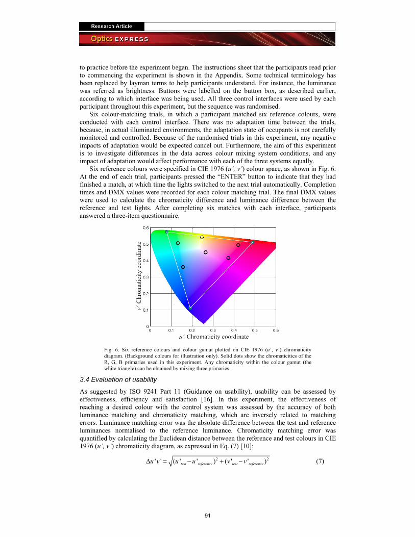
to practice before the experiment began. The instructions sheet that the participants read prior to commencing the experiment is shown in the Appendix. Some technical terminology has been replaced by layman terms to help participants understand. For instance, the luminance was referred as brightness. Buttons were labelled on the button box, as described earlier, according to which interface was being used. All three control interfaces were used by each participant throughout this experiment, but the sequence was randomised.

Six colour-matching trials, in which a participant matched six reference colours, were conducted with each control interface. There was no adaptation time between the trials, because, in actual illuminated environments, the adaptation state of occupants is not carefully monitored and controlled. Because of the randomised trials in this experiment, any negative impacts of adaptation would be expected cancel out. Furthermore, the aim of this experiment is to investigate differences in the data across colour mixing system conditions, and any impact of adaptation would affect performance with each of the three systems equally.

Six reference colours were specified in CIE 1976 (u’, v’) colour space, as shown in Fig. 6. At the end of each trial, participants pressed the “ENTER” button to indicate that they had finished a match, at which time the lights switched to the next trial automatically. Completion times and DMX values were recorded for each colour matching trial. The final DMX values were used to calculate the chromaticity difference and luminance difference between the reference and test lights. After completing six matches with each interface, participants answered a three-item questionnaire.

Fig. 6. Six reference colours and colour gamut plotted on CIE 1976 (u’, v’) chromaticity diagram. (Background colours for illustration only). Solid dots show the chromaticities of the R, G, B primaries used in this experiment. Any chromaticity within the colour gamut (the white triangle) can be obtained by mixing three primaries.

3.4 Evaluation of usability

As suggested by ISO 9241 Part 11 (Guidance on usability), usability can be assessed by effectiveness, efficiency and satisfaction [16]. In this experiment, the effectiveness of reaching a desired colour with the control system was assessed by the accuracy of both luminance matching and chromaticity matching, which are inversely related to matching errors. Luminance matching error was the absolute difference between the test and reference luminances normalised to the reference luminance. Chromaticity matching error was quantified by calculating the Euclidean distance between the reference and test colours in CIE 1976 (u’, v’) chromaticity diagram, as expressed in Eq. (7) [10]:

2 2' ' ( ' ' ) ( ' ' )test reference test referenceu v u u v vΔ = − + − (7)

91

Luminance and chromaticity coordinates were converted from the DMX values. The efficacy of the colour control interfaces is inversely related to the completion time, which was recorded during each task. Both effectiveness and efficacy are rather objective, but do not guarantee users satisfaction [17]. Jakob and Jonathan stated that, in 25% of their study cases, systems that the participants were most satisfied with were not the systems in which their performance was the best [18]. Thus, subjective assessment using questionnaires was also taken into account when evaluating usability.

3.5 Questionnaires

After the introduction, but before experiment starting, participants were asked: “If you had a chance to choose ONLY one interface to complete the colour-matching trials, which one would you choose?” This pre-experiment question aimed to understand users’ preference for these interfaces before actually using them.

After completing all matches for one interface, participants completed a three-item Likert questionnaire:

• “I am confident with the accuracy of my matches” (item 1)

• “I am satisfied with the speed with which I was able to make matches with this control system” (item 2)

• “Overall, I am satisfied with the ease of making the matches with this control system” (item 3).

Seven-point scales were used to describe the level of their agreement or disagreement with each of the three statements. A rating of seven was the most positive response, indicating “strongly agree” while a rating of one indicated “strongly disagree” [19].

4. Results Prior to beginning the experiment, 12 out of 18 (66.7%) participants believed that the RGB interface would be the easiest. This result is not surprising. The RGB interface appears to be more straightforward for inexperienced users than the other two and is likely familiar from the use of computer graphics software. However, results from both the psychophysical experiment and after-experiment-questionnaires contradict users’ initial opinion.

4.1 Control effectiveness

Chromaticity matching errors (Δ u’v’) for each trial were calculated using Eq. (7) and recorded. The mean chromaticity error and standard error of the mean (SEM) for each interface are shown in Fig. 7. Chromaticity matching errors with the RGB interface are significantly greater than with the other two interfaces. The results indicate no significant differences between the HSB and opponent colour interfaces.

92

Fig. 7. Chromaticity matching error (Δ u’v’) using different colour control interfaces. Circles show the mean Δ u’v’ and error bars show standard error of the mean (SEM).

Figure 8 shows the luminance matching error (ΔL) with the different interfaces. The RGB interface caused the greatest luminance matching errors, while HSB interface led to the smallest errors. The mean luminance matching error with the RGB interface was 70%. With the HSB interface, the luminance difference was more reasonable, with a mean of 26%. The mean luminance difference with the opponent colour interface was 38%.

Fig. 8. Luminance matching error (ΔL) for different colour control interfaces. Circles show the mean ΔL and error bars show standard error of the mean (SEM).

4.2 Control efficacy

Completion speed of the matching tasks, which is the inverse of the completion time, indicates the efficacy of a control system. Comparisons of speed or time in this experiment may introduce different biases against different interfaces. For instance, the RGB interface requires more button presses to adjust the luminance. Similarly, the efficiency of the hue settings with the HSB interface is dependent on the direct of travel selected by the participants. These issues, caused by the inherent nature of the interfaces, would also happen in real life. Thus, the comparison of completion time and speed can still be used to approximately evaluate the efficacy of a system. The completion time for each trial was recorded and the mean and SEM are shown in Fig. 9. When using the RGB interface, participants spent considerably more time to reach their desired colour than using the other interfaces. This indicates that the RGB interface was the least efficient interface among the three for the users to make their colour settings. The results showed no significant difference between HSB and opponent colour interfaces.

93

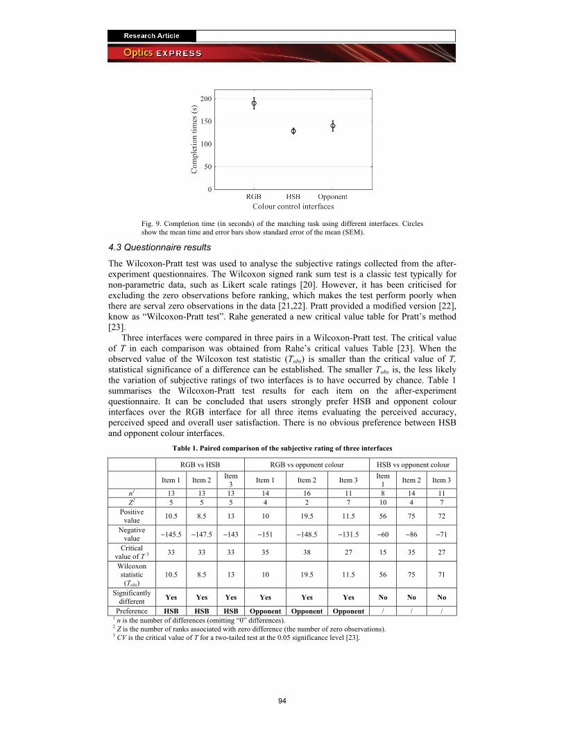
Fig. 9. Completion time (in seconds) of the matching task using different interfaces. Circles show the mean time and error bars show standard error of the mean (SEM).

4.3 Questionnaire results

The Wilcoxon-Pratt test was used to analyse the subjective ratings collected from the after- experiment questionnaires. The Wilcoxon signed rank sum test is a classic test typically for non-parametric data, such as Likert scale ratings [20]. However, it has been criticised for excluding the zero observations before ranking, which makes the test perform poorly when there are serval zero observations in the data [21,22]. Pratt provided a modified version [22], know as “Wilcoxon-Pratt test”. Rahe generated a new critical value table for Pratt’s method [23].

Three interfaces were compared in three pairs in a Wilcoxon-Pratt test. The critical value of T in each comparison was obtained from Rahe’s critical values Table [23]. When the observed value of the Wilcoxon test statistic (Tobs) is smaller than the critical value of T, statistical significance of a difference can be established. The smaller Tobs is, the less likely the variation of subjective ratings of two interfaces is to have occurred by chance. Table 1 summarises the Wilcoxon-Pratt test results for each item on the after-experiment questionnaire. It can be concluded that users strongly prefer HSB and opponent colour interfaces over the RGB interface for all three items evaluating the perceived accuracy, perceived speed and overall user satisfaction. There is no obvious preference between HSB and opponent colour interfaces.

Table 1. Paired comparison of the subjective rating of three interfaces

RGB vs HSB RGB vs opponent colour HSB vs opponent colour

Item 1 Item 2 Item

3 Item 1 Item 2 Item 3

Item 1

Item 2 Item 3

n1 13 13 13 14 16 11 8 14 11 Z2 5 5 5 4 2 7 10 4 7

Positive value

10.5 8.5 13 10 19.5 11.5 56 75 72

Negative value −145.5 −147.5 −143 −151 −148.5 −131.5 −60 −86 −71

Critical value of T 3

33 33 33 35 38 27 15 35 27

Wilcoxon statistic (Tobs)

10.5 8.5 13 10 19.5 11.5 56 75 71

Significantly different

Yes Yes Yes Yes Yes Yes No No No

Preference HSB HSB HSB Opponent Opponent Opponent / / / 1 n is the number of differences (omitting “0” differences). 2 Z is the number of ranks associated with zero difference (the number of zero observations). 3 CV is the critical value of T for a two-tailed test at the 0.05 significance level [23].

94

5. Discussion The comparison of the pre-experiment and after-experiment questionnaire is interesting. Before actually using the interfaces, most people (66.7%) believed that the RGB interface would be the easiest to reach the desired colours. However, in the experiment, it was the most difficult one. The RGB interface is often considered to be suitable for inexperienced users. The HSB and opponent colour interfaces are typically designed for professional users, such as lighting designers, since additional experience is presumably needed to operate them. For instance, the HSB interface requires users to be familiar with the sequence of hues on the colour wheel in order to quickly determine whether to move in a clockwise or anticlockwise rotation. The opponent colour interface requires the users to accept the concept that to decrease the proportion of one colour, one needs to increase the proportion of its opponent colour. However, this experiment demonstrated that inexperienced users were able to make their desired colour settings considerably faster with HSB and opponent colour interfaces, after a brief introduction, than with the more familiar RGB system.

One main difficulty when using the RGB interface is the control of luminance. Use of the RGB interface led to increased chromaticity matching errors, but the chromaticity differences, compared with the other interfaces, was not as great as the difference in luminance matching errors with the other interfaces. This suggests that the main drawback of the RGB interface is not in the control of chromaticity, but the control of luminance. As shown in Fig. 8, the mean ΔL with the RGB interface was 70%, but the mean of ΔL with the HSB interface was only 26%. In an earlier study with a similar experimental setup, but using a 3050 K white light, the mean illuminance matching error was found to be 18.5%, with the 95% confidence interval spanning 17.8% - 19.1%. This result was based on the data collected from 1440 trials [24]. In another experiment, in which participants viewed two lights (3050 K) directly and matched the luminance, the luminance difference was approximately 15% - 22% (95% confidence intervals) [25]. The RGB interface caused considerably higher luminance matching errors, presumably because few non-professional users can correctly adjust the luminance by controlling the intensity of three primaries, even though the method has been briefly described in the introduction. When using an RGB system, luminance co-varies with chromaticity, which can be confusing for some users.

Compared with earlier results of the white light experiments, the use of the HSB interface for coloured light has little negative impact on the luminance matching error. This interface appears to benefit from a separation in the control of luminance and chromaticity. The opponent colour interface led to greater luminance matching errors than HSB. This may be because inexperienced users cannot correctly distinguish the control of saturation and brightness when adjusting the output of the opponent channels. Users might adjust the luminance to change the saturation, which should be changed by adjusting the proportion of colours.

It is also worth noting that, regardless of which interface was used, the chromaticity matching errors were considerable greater than the just noticeable difference (JND). When Δu’v’ = 0.011, the chromaticity matching error is eleven times the just noticeable difference. It is not surprising that the acceptable chromaticity difference was much greater than detectable difference, since participants were told to complete the matching as accurate and as quickly as possible. In real life, users would likely not spend too much time with a control system to adjust the colour as well. Furthermore, in real illumination applications, users would likely be matching the colour of the light to a colour in their imagination, instead of to a neighbouring light source. The acceptable colour difference in real-life scenarios, with the use of a coloured light control system, would be expected to much greater than the JND. Further research to quantify the limits of acceptability would help to guide the design of the resolution of such a system.

Although the HSB interface is shown to be efficient, some improvements could still be made when designing an interface. To prevent the impact of additional light, self-luminous

95

control panels were excluded in this experiment. Thus, to reach a desired colour, participants had to press buttons many times if the target and starting hue angles were far apart. In real life, this could be easily improved by employing some technologies, such as a touch screen. The button box used in this experiment was a very simple input device. Buttons are not necessary for HSB control. Instead, a colour wheel or swatch panel could be used to allows users to select a hue. Slider bars, knobs, or other components on a touch screen could be used to adjust chroma and brightness. The information visualization, underlying technology, and holistic user experience would need to be considered before developing commercial products.

6. Conclusion Although participants may not necessarily be most satisfied with the system in which their performance was the best [18], users’ subjective ratings in this experiment were fully consistent with their performance, which leaves no doubt that the RGB interface has the lowest usability. The use of the RGB interface is time-consuming and ineffective – users were unable to reach their desired luminance. There was no significant preference shown in the experiment between HSB and opponent colour interfaces, but the latter did lead to greater luminance matching errors. The use of the HSB interface leads to the smallest luminance and chromaticity matching errors, suggesting this interface would enable users to easily reach their desired colour and brightness. New technologies could be combined with this interface to improve users’ experiences. Further studies could be conducted to investigate the magnitudes of perceptible and acceptable changes in light colour when using an HSB interface.

7. Appendix Pre-experiment introduction to the use of three interfaces:

You will be seated and viewing two identical booths illuminated by two lights. Each LED light has three single-colour channels. By mixing these three primary colours, a large number of colours can be created. In this experiment, your task is to use the control interface to match the colour and brightness of the light spot in the test booth with the one in the reference booth.

Throughout this experiment, you will use three different control interfaces. The ways in which these interfaces control light are:

• RGB (red, green and blue) colour mixing

• HSB (hue, saturation and brightness) specification

• Opponent colour mixing A label on the button box will indicate which interface is being used. Each section

includes six colour-matching trials. For each trial, press the ENTER button after you have made your match. Then, the experiment will switch to next trial automatically.

After completing six matches with one interface, you will complete a three-item questionnaire.

Description of three control interfaces When using the RGB (red, green and blue) interface, you will control intensity of each primary colour. As shown in Fig. 10, the first two buttons control the intensity of red light. The up arrow button increases the intensity, while the down arrow button decreases the intensity. The third and fourth buttons control the intensity of green light. Similarly, the fifth and sixth buttons control the intensity of blue light.

Light colour mixing is additive colour mixing, unlike the colour mixing of paints. For example, to get yellow light, you need to mix red and green light together. While mixing red

96

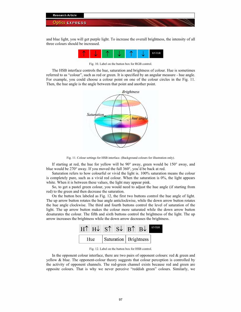
and blue light, you will get purple light. To increase the overall brightness, the intensity of all three colours should be increased.

Fig. 10. Label on the button box for RGB control.

The HSB interface controls the hue, saturation and brightness of colour. Hue is sometimes referred to as “colour”, such as red or green. It is specified by an angular measure - hue angle. For example, you could choose a colour point on one of the colour circles in the Fig. 11. Then, the hue angle is the angle between that point and another point.

Fig. 11. Colour settings for HSB interface. (Background colours for illustration only).

If starting at red, the hue for yellow will be 90° away, green would be 150° away, and blue would be 270° away. If you moved the full 360°, you’d be back at red.

Saturation refers to how colourful or vivid the light is. 100% saturation means the colour is completely pure, such as a vivid red colour. When the saturation is 0%, the light appears white. When it is between these values, the light may appear pink.

So, to get a pastel green colour, you would need to adjust the hue angle (if starting from red) to the green and then decrease the saturation.

On the button box labeled as Fig. 12, the first two buttons control the hue angle of light. The up arrow button rotates the hue angle anticlockwise, while the down arrow button rotates the hue angle clockwise. The third and fourth buttons control the level of saturation of the light. The up arrow button makes the colour more saturated while the down arrow button desaturates the colour. The fifth and sixth buttons control the brightness of the light. The up arrow increases the brightness while the down arrow decreases the brightness.

Fig. 12. Label on the button box for HSB control.

In the opponent colour interface, there are two pairs of opponent colours: red & green and yellow & blue. The opponent-colour theory suggests that colour perception is controlled by the activity of opponent channels. The red-green channel exists because red and green are opposite colours. That is why we never perceive “reddish green” colours. Similarly, we

97

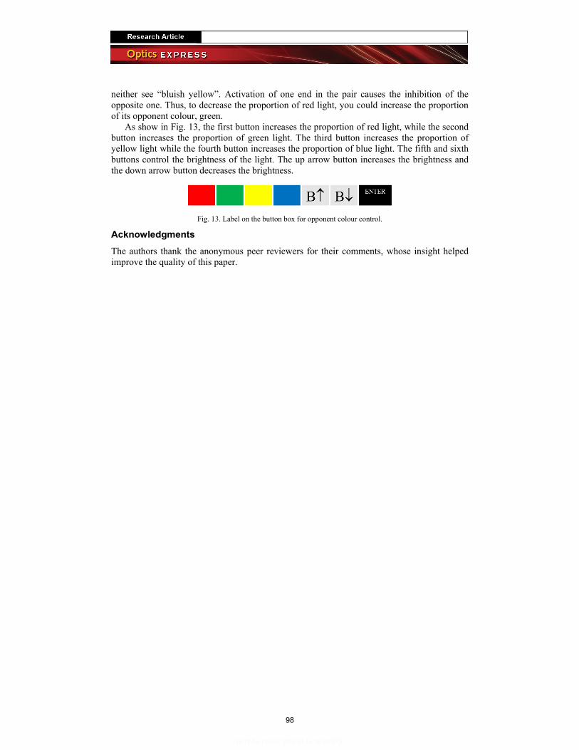
neither see “bluish yellow”. Activation of one end in the pair causes the inhibition of the opposite one. Thus, to decrease the proportion of red light, you could increase the proportion of its opponent colour, green.

As show in Fig. 13, the first button increases the proportion of red light, while the second button increases the proportion of green light. The third button increases the proportion of yellow light while the fourth button increases the proportion of blue light. The fifth and sixth buttons control the brightness of the light. The up arrow button increases the brightness and the down arrow button decreases the brightness.

Fig. 13. Label on the button box for opponent colour control.

Acknowledgments The authors thank the anonymous peer reviewers for their comments, whose insight helped improve the quality of this paper.

98

Chapter 6. The effect of control resolution on the usability of

colour-tunable LED lighting systems

99

The effect of control resolution on the usability of color-tunable lighting

systems

Wenye Hua* and Wendy Davisa aSchool of Architecture, Design and Planning, The University of Sydney, NSW 2006 *wenye.hu@sydney.edu.au

Color-tunable lighting systems with inappropriate resolutions may confuse end-

users and prevent them from easily specifying their desired colors. To improve

the design of color-tunable systems, a psychophysical experiment explored the

independent and interacting effects of hue, saturation and luminance control

resolutions on usability. Three criteria, efficiency, effectiveness and satisfaction,

were used to evaluate these effects. Results showed that combinations of middle

range hue resolution and saturation resolution facilitated the greatest usability.

When luminance control was independent of hue and saturation control,

luminance resolution did not impact the usability significantly.

Keywords: Controls; Behavioral Response; LED Sources and Systems; Color

Perception; Colorimetry

1. Introduction

Color-tunable LED lighting systems have become widespread in recent years. These systems

provide numerous color options. Many architects and designers have enthusiastically

embraced the freedom of design brought by the advanced lighting technologies. British

architect Terry Farrell affirmed that the recent explosion of technologies related to color and

light transferred the world “from a land of black and white to a wonderful new world; a world

that is in colour” [Farrell 2009]. Color-tunable lighting systems have been used in the iconic

Sydney Opera House [Julian and Lumascape 2016]. Mark Major stated that colored light was

usually employed to reinforce a particular idea in their projects, such as the Zollverein

Kokerei industrial complex in Germany and the Burj Al Arab tower in Dubai [Major 2009].

In the works of James Turrell, colored light occupies entire spaces to inspire observer’s

imagination and manipulate perception of light, space and time [Turrell 2017].

People’s preferences for color may not be universal. Culture, gender and age may all lead

to variations in color preference [Hurlbert and Ling 2007; McManus and others 1981; Ou and

100

others 2004a; 2004b]. An experiment with Arabic and English participants investigated the

impact of culture and gender on the color preference. Arabic participants preferred reddish

hues, while English participants preferred hues in the blue-green region of color space. The

difference in color preference between Arabic and English women was found to be greater

than the differences between the two groups of men [Al-Rasheed 2015]. Some researchers

suggested that color preference is determined by the emotions evoked by the colors or color

combinations [Ou and others 2004a; 2004b]. Color-tunable lighting systems, therefore, allow

diverse users to specify their desired light colors for particular spaces and situations.

In a color-tunable lighting system, high resolution is usually believed to be required

[Department of Energy n.d.], with “resolution” referring to the smallest change that can be

produced by a lighting control system. It is commonly accepted that low control resolutions,

which would not permit users to select their desired colors with great precision, would bring

dissatisfaction. A number of commercial products have been designed with high resolution.

Some manufacturers claim that their products offer more than 16 million color options

[Coghlan 2007; Halper 2017], while a few can even provide up to 3 × 1038 options

[Telelumen 2016]. However, the disadvantages of an extremely high resolution are not as

obvious as those of extremely low resolutions. Unlike the color selection tools or software

used for computer displays, interfaces of lighting control systems (LCSs) in the market are

usually small touch screens or smart phones. Most residential color-tunable products are

designed for non-expert users. Providing nearly infinite options does not ensure that a control

system provides an efficient and effective way for users to identify their desired colors.

Researchers found that small increments (high resolution) in a dimming system confused

users [Yılmaz and others 2016]. Inappropriate control resolution and complex user interfaces

may lead to end-user confusion, loss of productivity, and frustration. Negative experiences

might reduce the frequency with which a user interacts with the system.

A U.S. Department of Energy online report noted that user interfaces of color-tunable

lighting systems are more complicated than dimmers in white light systems. The report

suggests that users/owners may consider hiring a consultant, a trained facility manager or in-

house specialist to make changes to control system settings, since “the programming of the

controls may not be intuitive” [Department of Energy n.d.]. This might be a good strategy for

large-scale commercial projects, but cannot fulfill the increasing need for color-tunable

systems for residential and small-scale commercial applications.

Research has been conducted to better understand the effectiveness of lighting control

systems. Dugar and Donn suggested that numerous switching or dimming options (high

101

resolution) in white light systems could lead to wrong selections or create undesirable

atmospheres [Dugar and Donn 2011]. Chien and Mahdavi compared 12 commercial products

across three aspects (information types, control options, hardware) with seven criteria:

functional coverage, environmental information feedback, intuitiveness, mobility, network,

input, and output [Chien and Mahdavi 2008]. They intended for their study to serve as a

starting point for developing new generation user-interface models to promote the interaction

between users and environments. In another project, Dugar and his colleagues studied users’

interaction with four types of input interfaces: pushbutton, rotary, slide dimmer and screen-

based virtual interface. They found that users preferred remote interfaces and desired rich

interactive experiences with control systems [Dugar and others 2011].

However, there is a lack of scientific understanding of a fundamental issue underlying the

design of interactive LCSs: the relationship between the usability and the resolution of LCSs.

Understanding this topic not only requires skills in interface design/engineering, but also

deep knowledge of visual perception, color science and psychology. Limited interdisciplinary

research on this topic has been conducted systematically. This research draws from different

disciplines to evaluate the usability of LCSs with various resolutions. A previous study

showed that color control interfaces based on the three dimensions of hue, saturation and

brightness (HSB) yielded greater usability than the common red, green and blue (RGB)

control interface [Hu and Davis 2017]. This paper presents the results of an experiment

further characterizing the impact of hue, saturation and luminance resolutions on the

effectiveness and efficiency of color control and evaluating user satisfaction.

2. Methods

This experiment was conducted in a windowless dark room, in which the walls, ceiling and

floor were painted matte black. Two identical white booths were located side-by-side and

illuminated with identical luminaires – ETC Source Four LED Profile x7 Color System

luminaires. The reflectance of the surface of white booths is shown in Fig. 1. Four LED

channels were used to generate the light used in this experiment. They are red (peak

wavelength: 633 nm), green (peak wavelength: 523 nm), cyan (peak wavelength: 500 nm)

and blue (peak wavelength: 445 nm). The peak relative power of the green channel was

significantly lower than red and blue channels when all were set to the maximum DMX

values (255). Thus, the green and cyan channels were combined to provide green light. The

SPDs were added and the DMX signals sent to green and cyan channels were identical

throughout the experiment. Using this method, the four channels were reduced to three

102

primary channels, which will be simply referred to as the red, green and blue channels

hereafter.

During the experiment, these two LED luminaires were the only sources of light. The

experimental setup is shown in Fig. 2 and Fig. 3. Participants were seated one meter (~3’ 3”)

away from the front edge of the booths. They were instructed to use a button box to match the

colors of the illuminated circle on the lower surface of the test booth (right) with the color of

the illuminated circle on the target booth (left).

Fig. 1 The reflectance of the white panels used for the booths.

Fig. 2 Experimental setup. The left shows the elevation view and the right shows the

plan view of the setup.

103

Fig. 3 Experimental setup (from the observer’s back). General laboratory lights were

only on to capture the photographs. Participants were instructed to match the colors of

the illuminated circles on the lower surfaces of the booths.

Twenty subjects, 11 men and nine women, all with normal color vision, participated in the

experiment. They were instructed to complete a color matching task as quickly and

accurately as possible. They were all aware that the completion time and matching errors

were being recorded. At the end of each matching trial, they completed subjective ratings

about their experiences using the control system. The control interface, as shown in Fig. 4

was designed based on the hue, saturation and brightness (HSB) color system. Each button

increased or decreased one of these three dimensions of color, while the final button signaled

the end of the current trial and the beginning of the subsequent trial. Instructions and rating

scales were provided on paper. In this experiment, the brightness dimension of the control

system actually controlled the luminance in the middle of the illuminated circle on the lower

surface of each booth. To help the participants, who are all non-experts in lighting,

understand, the instructions and the button box label referred to “brightness.”

104

Fig. 4 The color control interface on the button box (23.8 cm in length, 16 cm in width

and 2.4 cm in depth). The first two buttons were used to increase and decrease the hue,

the third and fourth controlled the saturation, and the fifth and sixth controlled the

luminance. All labels, including the three-dimensional color space diagram, were

shown to the participants throughout the experiment.

The luminance for each DMX value, in intervals of 50 DMX units, was measured for each

channel, to obtain the relationship between luminance and DMX value. With the functions

obtained by fitting the data, shown in Fig. 5, luminance was calculated from the DMX values,

which were specified and recorded during the experiment.

Fig. 5 Luminance as a function of DMX value for each color channel and each

luminaire. Dashed lines show the relationship between luminance and DMX values for

the luminaire used in the test booth, while solid lines show the data for the luminaire

used in the target booth.

105

The spectral power distribution (SPD) of each single colored light channel of each

luminaire was measured at every step (50 DMX unit intervals) of the DMX values. The SPDs

of the target luminaire and test luminaire were slightly different. Figure 6 shows the SPDs of

each channel of the target light and the test light source.

Fig. 6 Relative power as a function of wavelength for the luminaires used in the target

booth (a) and test booth (b).

To develop a color-tunable control system for this experiment, colorimetric parameters

(CIE 1976 L*, a*, b*) and photometric parameters (luminance) of any colored light need to be

associated with the device-specific control signal information (DMX values). The method for

converting DMX values to tristimulus values (X, Y, Z) was reported in detail in a previous

publication [Hu and Davis 2017]. Since the SPDs of two LED luminaires were slightly

different, as shown in Fig. 6, the colorimetric computations were performed separately based

on the measurements of each luminaire. After obtaining tristimulus values, CIE 1976 L*, a*,

b* (CIELAB) coordinates were calculated, with an equal-energy radiator (x=0.333, y=0.333)

of the maximum luminance as the selected white point (Xn, Yn and Zn). Then, the a* and b*

coordinates were converted to hue and saturation. The relationship between DMX values and

CIELAB coordinates was used to create all lighting conditions in the experiment, as DMX

values can be determined for colored light of any set of CIELAB coordinates, L*, a*, b*.

Before conducting the experiment, an understanding of observers’ perceptions of color

differences was needed. The control system’s resolution should, theoretically, be higher than

the just noticeable difference (JND) and lower than the just acceptable difference. A two-

alternative-forced-choice (2AFC) experiment was used to measure the JND for luminance,

which was found to be 12.4 %. A previous study with similar experimental conditions

indicates that illuminance differences of ~ 20 % of the reference are acceptable to observers

106

[Hu and Davis 2016a]. So, in this experiment, the test luminance resolution (LR) was set to

be 0.75 (9.3 %), 1 (12.4 %), 1.25 (15.5 %) and 1.5 (18.6 %) times the luminance JND.

Equations (1-2) show two ways of calculating CIELAB color difference [CIE 2004; Ohta

and Robertson 2006; Schanda 2007]. The JNDs for hue and saturation were determined by

∆E*ab, which is the Euclidean distance in CIELAB and is approximately proportional to

perceived color differences [Schanda 2007]. A JND for color is considered be approximately

∆E*ab=1.0 [Hunt and Pointer 2011]. The range of test resolutions for hue and saturation were

determined with preliminary testing of three participants. Levels of hue resolution (HR) and

saturation resolution (SR) were 1, 3, 5, and 7 times the JND (∆E*ab=1.0) for hue or saturation.

High values for HR, SR or LR correspond to coarse control resolution; low values correspond

to fine control resolution.

In this experiment, the saturation dimension and hue dimension were operationally defined

as the chroma (saturation) and hue angle (hue) in CIELAB color space [Schanda 2007].

Equations (3-4) were used in this experiment to convert CIE 1976 chromaticity coordinates

L*, a*, b* to the chroma and hue angle. CIE 1976 chroma (C*ab) is the distance from the origin

to the given point, while hue angle (hab) is specified by an angular measure.

∆𝐸#$∗ = '(∆𝐿∗)+ + (∆𝑎∗)+ + (∆𝑏∗)+ ( 1 )

∆𝐸#$∗ = '(∆𝐿∗)+ + (∆𝐶#$∗ )+ + (∆𝐻#$∗ )+ ( 2 )

where

𝐶#$∗ = '𝑎∗+ + 𝑏∗+ ( 3 )

ℎ#$ = tan56(𝑏∗ 𝑎∗⁄ ) ( 4 )

When a single dimension of color was adjusted by a user, the other two dimensions

remained constant. For instance, when the “Saturation +” button was pressed, the color of the

illuminated circle in the test booth would change from the starting CIELAB coordinates (e.g.

color 0) to new coordinates (e.g. color 1), as shown in Fig. 7 (a). For this button press, the

chroma of the color increased by the given SR, while the hue angle and the luminance of the

color remained the same. When the “Hue +” button was pressed, the chroma and luminance

would remain constant and the hue angle would be increased counterclockwise. The CIELAB

107

coordinates of the light in the test booth would change from the starting point (e.g., color 0)

to a new point (e.g., color 1), as shown in Fig. 7 (b).

Fig. 7 (a) When the “Saturation +” button was pressed, the CIELAB coordinates of the

test color changed from point “color 0” to point “color 1,” with a saturation increment

of the given saturation resolution, while the luminance and hue angle of the color

remained constant. (b) When the “Hue +” button was pressed, the CIELAB coordinates

of the color changed from point “color 0” to point “color 1,” with a hue change of the

given hue resolution, while the luminance and chroma of the test color remained

constant.

The CIELAB coordinates of the new color (color 1) after a change in chroma can be

mathematically expressed as (5-6), where a*0 and b*0 are the CIELAB coordinates of the

initial color, a*1 and b*1 are the coordinates of the new color, SR is the saturation resolution

and h0 is the hue angle, in radians, of both colors.

𝑎6∗ = 𝑎8∗ + 𝑆𝑅 × cos ℎ8 ( 5 )

𝑏6∗ = 𝑏8∗ + 𝑆𝑅 × sin ℎ8 ( 6 )

When controlling the hue dimension, the chroma of the color remains constant, thus, C*ab,1

= C*ab,0. Setting the hue difference between two colors ∆*Hab=HR and rearranging (7) [Ohta

and Robertson 2006; Schanda 2007], the hue of a color after a change in hue can be

determined by (8). The CIELAB coordinates of the new color (color 1) can be further

obtained.

108

∆𝐻#$∗ = 2 ×'𝐶#$,6∗ × 𝐶#$,8∗ × sin(∆ℎ#$ 2⁄ ) ( 7 )

∆ℎ#$ = 2 × sin56 B CD+×EFG,H

∗ I ( 8 )

A three-factors four-levels (43) full factorial experimental design [Box and others 2005]

was used and observers completed color matching task for all 64 conditions (four levels of

three dimensions), in a randomized sequence. The CIELAB coordinates L*, a*, and b* of the

five target colored lights are presented in Table A1 in the Appendix. In each trial, one of the

target colors was randomly presented and the presentation of test color was pseudo-random.

All test colors started the same distance (∆E*ab=20), in a random direction, from the selected

target color in CIELAB. This was done to ensure relatively unbiased comparisons across

trials and limit the magnitude of hue differences.

The usability of the LCSs was evaluated according to ISO 9241 Part 11 (Guidance on

usability) [Standardization 1998], by measuring effectiveness, efficiency, and users’

satisfaction. In this experiment, effectiveness was inversely assessed by calculating the color

differences between the target and test colors in CIELAB (∆E*ab) at the conclusion of each

trial, using (9).

∆𝐸#$∗ = JK𝐿∗LMNL − 𝐿∗L#PQMLR++ K𝑎∗LMNL − 𝑎∗L#PQMLR

++ K𝑏∗LMNL − 𝑏∗L#PQMLR

+ (9)

Efficiency was inversely assessed by measuring the time required to complete the

matching task. Satisfaction was evaluated with a seven-point rating scale, with a rating of

seven indicating strong agreement with the statement, “Overall, I am satisfied with the ease

of making the matches with this control system.”

3. Results

Data from eleven trials were excluded due to unexpected button box disconnections and

accidental terminations of trials when participants pressed the “Enter” button that signals the

end of a trial unintentionally. Although participants practiced using the control system before

data were collected, the first few trials were still impacted by their unfamiliarity with the

system. After completing the experiment, several participants requested that the experimenter

excluded data from their first few trials, due to their unfamiliarity with the system. The

109

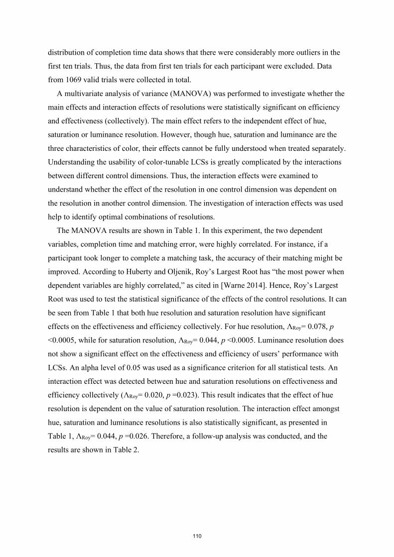
distribution of completion time data shows that there were considerably more outliers in the

first ten trials. Thus, the data from first ten trials for each participant were excluded. Data

from 1069 valid trials were collected in total.

A multivariate analysis of variance (MANOVA) was performed to investigate whether the

main effects and interaction effects of resolutions were statistically significant on efficiency

and effectiveness (collectively). The main effect refers to the independent effect of hue,

saturation or luminance resolution. However, though hue, saturation and luminance are the

three characteristics of color, their effects cannot be fully understood when treated separately.

Understanding the usability of color-tunable LCSs is greatly complicated by the interactions

between different control dimensions. Thus, the interaction effects were examined to

understand whether the effect of the resolution in one control dimension was dependent on

the resolution in another control dimension. The investigation of interaction effects was used

help to identify optimal combinations of resolutions.

The MANOVA results are shown in Table 1. In this experiment, the two dependent

variables, completion time and matching error, were highly correlated. For instance, if a

participant took longer to complete a matching task, the accuracy of their matching might be

improved. According to Huberty and Oljenik, Roy’s Largest Root has “the most power when

dependent variables are highly correlated,” as cited in [Warne 2014]. Hence, Roy’s Largest

Root was used to test the statistical significance of the effects of the control resolutions. It can

be seen from Table 1 that both hue resolution and saturation resolution have significant

effects on the effectiveness and efficiency collectively. For hue resolution, ΛRoy= 0.078, p

<0.0005, while for saturation resolution, ΛRoy= 0.044, p <0.0005. Luminance resolution does

not show a significant effect on the effectiveness and efficiency of users’ performance with

LCSs. An alpha level of 0.05 was used as a significance criterion for all statistical tests. An

interaction effect was detected between hue and saturation resolutions on effectiveness and

efficiency collectively (ΛRoy= 0.020, p =0.023). This result indicates that the effect of hue

resolution is dependent on the value of saturation resolution. The interaction effect amongst

hue, saturation and luminance resolutions is also statistically significant, as presented in

Table 1, ΛRoy= 0.044, p =0.026. Therefore, a follow-up analysis was conducted, and the

results are shown in Table 2.

110

Table 1. MANOVA results. Significance of main and interaction effects on efficiency

and effectiveness collectively was tested using Roy's Largest Root. The rows of hue

resolution, saturation resolution and luminance resolution show the significance of

independent main effects of each resolution and the rows with “×” show the

significance of interaction effects between two or more resolutions.

Effect

Value

F

Hypothesis df

Error df

Sig.

Partial η2

Intercept 2.543 1249.641b 2.000 983.000 .000 .718 Hue resolution .078 25.581c 3.000 984.000 .000 .072 Saturation resolution .044 14.373c 3.000 984.000 .000 .042 Luminance resolution .002 .611c 3.000 984.000 .608 .002 Hue resolution × Saturation resolution .020 2.153c 9.000 984.000 .023 .019

Hue resolution × Luminance resolution .003 .322c 9.000 984.000 .968 .003

Saturation resolution × Luminance resolution .008 .923c 9.000 984.000 .504 .008

Hue resolution × Saturation resolution × Luminance resolution

.044 1.611c 27.000 984.000 .026 .042

As shown in Table 2, the main effects of hue resolution were significant on both efficiency

(F [3, 984] = 25.266, p <0.0005) and effectiveness (F [3, 984] = 2.923, p =0.033). Similarly,

saturation resolution yielded significant main effects on both efficiency (F [3, 984] = 13.533,

p <0.0005), and effectiveness (F [3, 984] = 5.368, p =0.001). Hue resolution had noticeably

more impact on efficiency (partial η2=0.072) than effectiveness (partial η2 =0.009).

Saturation resolution also had more effect on efficiency (partial η2=0.040) than on

effectiveness (partial η2=0.016).

111

Table 2. The results of follow-up analysis of variance (ANOVA). The significance of

the main and interaction effects of resolution on efficiency and effectiveness. The

completion time rows show the significance of effects on efficiency, which is inversely

assessed by the completion time. The matching error rows show the significance of

effects on effectiveness, which is inversely assessed by matching errors. Similar to

Table 1, the rows with “×” show the significance of interaction effects between two or

more resolutions.

Source Dependent Variable

Type III Sum of Squares df Mean Square F Sig.

Partial η2

Corrected Model Completion time 416532.279a 63 6611.623 2.944 .000 .159 Matching error 13115.970b 63 208.190 1.138 .220 .068

Intercept Completion time 3930001.112 1 3930001.112 1749.805 .000 .640 Matching error 204849.393 1 204849.393 1119.950 .000 .532

Hue resolution Completion time 170240.454 3 56746.818 25.266 .000 .072 Matching error 1603.904 3 534.635 2.923 .033 .009

Saturation resolution

Completion time 91183.783 3 30394.594 13.533 .000 .040 Matching error 2945.613 3 981.871 5.368 .001 .016

Luminance resolution

Completion time 3111.252 3 1037.084 .462 .709 .001 Matching error 160.586 3 53.529 .293 .831 .001

Hue resolution × Saturation resolution

Completion time 43285.509 9 4809.501 2.141 .024 .019 Matching error 1129.081 9 125.453 .686 .722 .006

Hue resolution × Luminance resolution

Completion time 6068.346 9 674.261 .300 .975 .003 Matching error 500.114 9 55.568 .304 .974 .003

Saturation resolution × Luminance resolution

Completion time 16910.355 9 1878.928 .837 .582 .008 Matching error

1088.888 9 120.988 .661 .744 .006

Hue × Saturation × Luminance resolution

Completion time 81154.901 27 3005.737 1.338 .117 .035 Matching error 5844.186 27 216.451 1.183 .238 .031

Error Completion time 2210029.788 984 2245.965 Matching error 179982.911 984 182.909

Total Completion time 6684432.604 1048 Matching error 405758.888 1048

Corrected Total Completion time 2626562.066 1047 Matching error 193098.880 1047

a. R2 = .159 (Adjusted R Squared = .105) b. R2 = .068 (Adjusted R Squared = .008)

112

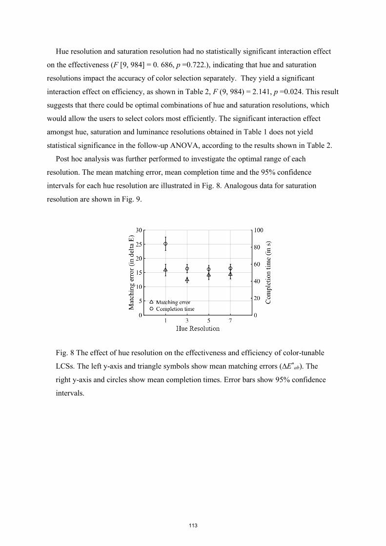
Hue resolution and saturation resolution had no statistically significant interaction effect

on the effectiveness (F [9, 984] = 0. 686, p =0.722.), indicating that hue and saturation

resolutions impact the accuracy of color selection separately. They yield a significant

interaction effect on efficiency, as shown in Table 2, F (9, 984) = 2.141, p =0.024. This result

suggests that there could be optimal combinations of hue and saturation resolutions, which

would allow the users to select colors most efficiently. The significant interaction effect

amongst hue, saturation and luminance resolutions obtained in Table 1 does not yield

statistical significance in the follow-up ANOVA, according to the results shown in Table 2.

Post hoc analysis was further performed to investigate the optimal range of each

resolution. The mean matching error, mean completion time and the 95% confidence

intervals for each hue resolution are illustrated in Fig. 8. Analogous data for saturation

resolution are shown in Fig. 9.

Fig. 8 The effect of hue resolution on the effectiveness and efficiency of color-tunable

LCSs. The left y-axis and triangle symbols show mean matching errors (∆E*ab). The

right y-axis and circles show mean completion times. Error bars show 95% confidence

intervals.

113

Fig. 9 The effect of saturation resolution on the effectiveness and efficiency of color-

tunable LCSs. The left y-axis and triangle symbols show mean matching errors (∆E*ab).

The right y-axis and circle symbols show mean completion times. Error bars show 95%

confidence intervals.

To identify the optimal resolution range, homogenous subsets tests were used to examine

the differences between groups, as shown in Tables 3, 4 and 5. It can be seen from Fig. 8 and

Table 3 that the extremely fine hue resolution (HR=1) leads to notably increased completion

times and matching errors. At coarser resolutions (HR≥3), hue resolution does not have

significant impact on completion time. One middle range resolution (HR=3) leads to the

greatest matching accuracy. These results suggest that fine hue resolution, of which the

magnitude of change is close to JND, should be avoided when designing color-tunable LCSs.

As shown in Fig. 9, which plots matching errors and completion times as a function as

saturation resolutions, the middle range saturation resolutions are associated with high

effectiveness and efficiency. It can be seen in Tables 4 and 5 that extremely fine saturation

resolution (SR=1) leads to significantly increased completion times and extremely coarse

saturation resolution (SR=7) causes more matching errors. To improve the usability of LCSs,

saturation resolution should be in a middle range (3≤SR≤5).

114

Table 3. Mean completion time for each hue resolution level in homogeneous subsets.

Means categorized in different subsets are considered significantly different. HR=1

leads to significantly longer completion time.

Hue resolution

(HR) Mean completion time

Subset 1 Subset 2 5.0 53.92 s 3.0 54.75 s 7.0 55.02 s 1.0 83.90 s

Table 4. Mean completion time for each saturation resolution level in homogeneous

subsets. Means categorized in different subsets are considered significantly different.

SR=1 leads to significantly longer completion time, while SR=5 & 3 lead to shorter

time.

Saturation resolution

(SR) Mean completion time

Subset 1 Subset 2 Subset 3 5.0 51.06 s 3.0 56.94 s 56.94 s 7.0 64.92 s 1.0 77.41 s

Table 5. Mean matching error for each saturation resolution level in homogeneous

subsets. Means categorized in different subsets are considered significantly different.

SR=1& 7 cause significantly greater matching errors, while SR=3 & 5 lead to smaller

errors.

Saturation resolution

(SR) Mean matching error

Subset 1 Subset 2 3.0 ∆E*ab = 12.72 5.0 ∆E*ab = 12.76 1.0 ∆E*ab = 14.77 ∆E*ab = 14.77 7.0 ∆E*ab = 16.83

Interactions between two control dimensions were analyzed in pairs: hue and saturation,

luminance and saturation, and hue and luminance. However, as shown in Table 2, only hue

and saturation resolutions yield statistically significant interaction effect on efficiency, F (9,

984) = 2.141, p =0.024. The mean completion times and 95% confidence intervals for all

combinations of hue and saturation resolutions, as listed in Table 6, were calculated to

115

identify the optimal combinations that may benefit users by enabling more efficient colors

selections. Means and 95% confidence intervals are visualized in a three-dimensional graph

in Fig. 10. When both hue and saturation resolutions were in the middle range, participants

spent less time completing the color matching tasks. Three combinations of hue and

saturation resolutions, HR=3 VR=5, HR=5 VR=5, and HR=5 VR=3, lead to significantly

faster completions, which indicates that they may be optimal resolution combinations for

LCSs.

Table 6. A comparison of mean completion times with 95% CIs for all combination of

every level of hue and saturation resolution.

Hue resolution

Saturation resolution

Mean (s)

Std. Error (s)

95% Confidence interval Lower bound

(s) Upper bound

(s)

1.0

1.0 100.99 5.90 89.40 112.57 3.0 71.52 5.54 60.65 82.40 5.0 67.42 5.79 56.07 78.78 7.0 95.75 5.82 84.32 107.18

3.0

1.0 68.79 6.86 55.33 82.26 3.0 56.75 6.11 44.76 68.74 5.0 41.45 5.99 29.70 53.21 7.0 53.69 6.19 41.55 65.83

5.0

1.0 77.64 5.86 66.14 89.14 3.0 40.77 5.75 29.48 52.06 5.0 42.05 5.83 30.61 53.49 7.0 56.82 5.71 45.61 68.03

7.0

1.0 58.01 6.17 45.90 70.13 3.0 56.32 5.67 45.20 67.44 5.0 52.26 5.75 40.98 63.53 7.0 52.0 5.81 40.59 63.40

116

Fig. 10 Interaction between hue and saturation resolutions on completion times.

Columns show mean completion times for the combinations of each hue and saturation

resolution level.

The ordinal data that came from questionnaire ratings were analyzed using a series of

Mann-Whitney U-tests, which are the equivalent of t-tests for non-parametric data. To

examine the statistical significance, ratings for every two levels in each dimension were

compared in pairs and the results are summarized in Table 7. The medians and 95%

confidence intervals of the subjective ratings are shown in Table A2 in the Appendix. Table 7

shows that an extremely fine hue resolution (HR=1) leads to significantly more

dissatisfaction than other hue resolutions (p = 0, 0, 0.004 when compared with HR=3, 5, 7

respectively). The satisfactions ratings for the middle and coarse range hue resolutions

(HR=3, 5, 7) were not significantly different. An extremely fine saturation resolution (SR=1)

leads to the least satisfaction (p = 0, 0, 0 when compared with SR=3, 5, 7 respectively). Users

were significantly more satisfied with one middle-range resolution (SR=5) than the extremely

coarse saturation resolution (SR=7), as revealed in Table 7, U = 30977, p = 0.016. There is no

statistically significant effect of luminance resolutions on the subjective ratings.

117

Table 7. Summary of the results of the Mann-Whitney U-tests. The significance of the

differences in subjective ratings between every two levels was examined for each

resolution. For instance, the first column shows that the subjective ratings for HR=1 are

significantly different from the ratings for HR=3. The difference between ratings for

SR=1 and SR=3 are significantly different as well, while LR=9.3 % and LR=12.4 %

were not rated significantly differently.

Hue resolution (HR)

HR=1 vs

HR=3

HR=1 vs

HR=5

HR=1 vs

HR=7

HR=3 vs

HR=5

HR=3 vs

HR=7

HR=5 vs

HR=7 Mann-Whitney U 25950.5 28909.5 31262 31237 29909.5 33333.5 Wilcoxon W 63625.5 66584.5 68937 59440 65420.5 68844.5 Z -3.988 -4.559 -2.906 -0.546 -1.014 -1.545 Asymp. Sig. (2-tailed) 0.000 0.000 0.004 0.585 0.311 0.122

Saturation resolution (SR)

SR=1 vs

SR=3

SR=1 vs

SR=5

SR=1 vs

SR=7

SR=3 vs

SR=5

SR=3 vs

SR=7

SR=5 vs

SR=7 Mann-Whitney U 25339.5 22954.5 26274 34234 34101 30977 Wilcoxon W 55229.5 52844.5 56164 71909 69081 65957 Z -4.841 -5.823 -3.65 -1.252 -1.174 -2.407 Asymp. Sig. (2-tailed) 0.000 0.000 0.000 0.211 0.24 0.016

Luminance resolution (LR)

LR=9.3 % vs

LR=12.4 %

LR=9.3 % vs

R=15.5 %

LR=9.3% vs

LR=18.6 %

LR=12.4 % vs

LR=15.5 %

LR=12.4 % vs

LR=18.6 %

LR=15.5 % vs

LR=18.6 % Mann-Whitney U 31861 32932.5 33397.5 33114.5 33658.5 35623.5 Wilcoxon W 65531 64810.5 65275.5 66784.5 67328.5 70868.5 Z -0.473 -0.276 -0.517 -0.709 -0.904 -0.237 Asymp. Sig. (2-tailed) 0.636 0.783 0.605 0.478 0.366 0.813

4. Discussion

In a previous study, luminance resolution had an impact on the usability of a white light LCS

designed solely for changing luminance [Hu and Davis 2016b]. The luminance resolutions

used in this experiment did not show significant effects on the efficiency, effectiveness and

118

satisfaction. For the LCS used in this experiment, DMX signals needed to be specified based

on physical measurements of the light. Therefore, luminance, a physical property that is

measurable and additive in color mixing calculations, was used instead of brightness, which

is an immeasurable psychological attribute of visual perception. The luminance should be,

theoretically, independent of the colors of the light. Luminance accounts for the differences

in the color of light. Thus, white light was used to simplify the measurement and exclude the

possible psychological effects of colored light. The JNDs for luminance were obtained with a

2AFC preliminary experiment, in which participants compared the luminances of white light

in the target and test booths. The results showing that luminance resolution does not have a

significant effect might suggest that the psychological effects of colored light should be taken

into consideration. In the future, if methods were to be developed that additively predict

brightness perception, brightness JNDs for individual colors could be used to investigate the

impact of brightness resolution. It is also possible that luminance resolutions beyond the

range examined in this experiment would demonstrate a stronger effect on usability.

In this experiment, CIELAB was used to calculate the color differences between the target

and test colors. CIELAB is not a perfectly uniform color space. Some alternative color

difference equations in more uniform color spaces have been developed, such as

CIEDE2000. However, the CIEDE2000 color-difference formula is recommended for color

differences less than 5.0 CIELAB units (∆E*ab) since, when the difference is greater than 5.0

units (∆E*ab ≥5.0), the computation discontinuity in CIEDE2000 color-difference is not

negligible [Melgosa, 2006; Melgosa et al., 2017; Sharma, Wu, & Dalal, 2005; Sharma, Wu,

Dalal, & Celik, 2004]. The median of acceptable color differences studied in this experiment

was 11 CIELAB units (∆E*ab =11), so CIEDE2000 would be inappropriate for this

experiment. In one study, five color difference measurement methods (∆E*ab, ∆E94, ∆E00,

∆ECMC and ∆EDIN99) were compared to determine which best correlates with perceived color

differences. Ten Pantone color samples were selected as the reference colors. Each sample

was compared with four other color samples, each of which had a color difference of 6 units

(∆E*ab =6.0±0.5). The results showed that “there is no clear winner for a color difference

equation that outperforms the rest” [Millward, 2009]. As Melgosa et al [2017], state, “It must

be said that since this time (1976) CIELAB has been very successful and widely employed in

basic and applied research.” Additionally, the objective of this experiment was to compare

the effectiveness of LCSs using the matching errors as a measure. It was not concerned with

the actual values of the perceived color differences.

119

The results of the subjective ratings show a possible centering bias, as participants tended

to choose the middle range ratings in the evaluations. Although this full factorial experiment,

comparing 64 conditions at one time, was an efficient way to test the significant factors, a

large number of repeating tasks might have made participants less sensitive to their

experiences of using the LCS. Additionally, in the interest of time, in this experiment, there

was only one item in the questionnaire addressing overall satisfaction. In future studies,

researchers could narrow down the testing range of resolution based on the results of this

experiment and design more evaluation items to assess different aspects of user satisfaction.

For instance, a questionnaire widely used in computer usability assessments could be adopted

[Lewis 1991].

When hue and saturation resolutions were both the same, the magnitudes of changes in

hue and saturation were approximately perceptually equal. It might be easier for users to

learn and predict the pattern of changes when using LCSs with similar hue and saturation

resolutions than when these dimensions change in vastly different ways. Observations made

during experiment suggest that most participants prioritized the adjustment of hue over

saturation. It was common for users to adjust the hue of test light close to the target color and

then adjust the saturation. Users seemed to understand the concept of hue better than the

concept of saturation. During the experiment, they were able to correctly judge hue

differences between the target and test colors and then make adjustment correctly. However,

sometimes participants mistakenly believed that a large saturation difference was due to a

luminance or hue difference. For instance, participants occasionally adjusted the luminance to

attempt to compensate for a saturation difference.

The results reveal that users’ behaviors when using color-tunable systems vary radically.

The mean completion times for some participants were up to 98.45 s and 92.38 s, while for

some others, the means were only 38.94 s and 38.58 s. Similarly, some participants were able

to match the colors more accurately (∆E*ab =8.38 in average) than the others (∆E*ab =16.64 in

average). It is easy to understand that, in a variety of situations, some users tend to make a

setting quickly, while some others may be more hesitant. This difference suggests that

manufacturers may consider developing different interfaces for customers with different

habits and approaches to adjusting the lighting.

In this experiment, the color-matching task was used to simulate a scenario in which

people use a color-tunable system to adjust the light to correspond to their desired color. The

matching errors were used as a measure to compare how well LCSs with various resolutions

allow users to select color accurately. The final settings are indicative of users’ acceptable

120

color difference, which are independent of the magnitude of their perceived color differences.

Due to the experimental setup, the background of the two circles in the booths was

illuminated by spill/reflected light from the luminaires. The colors of background appeared

relatively similar to the colors of circles and changed with the circle colors accordingly. A

crispening effect may occur, which causes an “increase in the perceived magnitude of color

differences” [Fairchild 2013]. This phenomenon, as well as the direct comparison enabled by

the side-by-side booth layout, could make participants more sensitive to the color differences

than they’d be in a real-world setting. Nonetheless, the median matching errors in this

experiment (∆E*ab=11) show that the acceptable color differences are much greater than the

perceived color differences.

5. Conclusions

One aim of this research is to identify optimal ranges of control resolutions, to guide the

design of color-tunable LCSs. High usability is achieved when hue resolution is ∆E*ab=3 and

saturation resolution is ∆E*ab=5 (HR=3 and SR=5). The luminance resolution of a color-

tunable LCS in the examined range (9.3 %-18.6 %) does not appear to impact the usability of

the system significantly. Most users adjusted hue first and the concept of saturation was not

as well understood as the concept of hue. Even after thorough training sessions, participants

still seemed to experience a bit of confusion when controlling the saturation dimension.

When designing the interface of LCSs for real products, the hue control dimension should be

prioritized and users should be provided with comprehensible visualizations of the saturation

control dimension.

If designing a color-tunable LED system for applications that do not require accurate color

settings, such as residential applications, low-resolution systems with coarse hue and

saturation resolutions (the combination of HR=7 and SR=7 or the combination of HR=7 and

SR=5) would likely be acceptable. One additional advantage of LCSs with HR=7 and SR=7

is the magnitudes of changes are approximately equally perceived.

It is worth noting that all studies of usability are greatly complicated by the effects of

different variables, such as user interfaces, instructions for use, etc, and the possible

interactions amongst them. User interface design includes a large number of attributes, such

as the graphic design, the types of input devices, etc. Effective instructions need to be

developed for users, with consideration of potential costumers' gender, age, background, etc.

To better understand these complex interactions, the individual effects of each factor needs to

be explored. This research, which solely investigated the effect of resolution, is just a step

121

towards a better understanding of usability of lighting control systems. This research does not

provide a universal solution for all LCSs.

Disclosure statement

The authors report no declarations of interest.

122

References

1 Farrell T. Colour for Architecture Today. New York: Taylor & Francis Ltd; 2009. 192 p. 2 Julian W, Lumascape. The Sydney opera house concert hall celebrates two years of LEDs.

Lighting 2016;36(4):26-27. 3 Major M. Architectural light and colour as a source of inspiration: an apporoach to the use

of colour. In: Mikellides TPB, editor. Colour for Architecture Today. New York:

Taylor & Francis Ltd; 2009. p. 151-158. 4 Turrell J. Architectural light. 2017, [accessed 2017 20 Sep].

http://jamesturrell.com/work/type/architectural-light/ 5 Hurlbert AC, Ling Y. Biological components of sex differences in color preference. Curr

Biol. 2007;17(16):R623-R625. 6 McManus I, Jones AL, Cottrell J. The aesthetics of colour. Perception. 1981;10(6):651-666. 7 Ou L-C, Luo MR, Woodcock A, Wright A. A study of colour emotion and colour

preference. Part I: Colour emotions for single colours. Color Res Appl. 2004

a;29(3):232-240. 8 Ou L-C, Luo MR, Woodcock A, Wright A. A study of colour emotion and colour

preference. Part II: Colour emotions for two-colour combinations. Color Res Appl.

2004;29(4):292-298. 9 Al-Rasheed AS. An experimental study of gender and cultural differences in hue

preference. Front Psychol. 2015;6(30). 10 Department of Energy. n.d. Understanding led color-tunable products. Office of energy

efficiency & renewable energy [accessed 2017 20 Sep].

https://energy.gov/eere/ssl/understanding-led-color-tunable-products 11 Coghlan A. It's lights out for household classic. New Sci. 2007;193(2597):26-27. 12 Halper M. 2017 September 18. Philips turns modern Hanoi bridge into a colorful light

display. LEDs Magazine. [accessed 2017 September 18].

http://www.ledsmagazine.com/articles/2017/07/philips-turns-modern-hanoi-bridge-

into-a-colorful-light-display.html. 13 Telelumen. 2016 6/12. Products. [accessed 2016 6/12].

http://www.telelumen.com/products2.html. 14 Yılmaz F, Ticleanu C, Howlett G, King S, Littlefair P. People-friendly lighting controls–

User performance and feedback on different interfaces. Lighting Res. Technol.

2016;48(4):449-472.

123

15 Dugar AM, Donn MR. Tangible intervention- Improving the effectiveness of lighting

control systems. Lighting Res. Technol. 2011; 43: 381–393 2011. 16 Chien S, Mahdavi A. Evaluating interface designs for user-system interaction media in

buildings. Adv Eng Inform. 2008;22(4):484-492. 17 Dugar AM, Donn MR, Osterhaus W. Tangible lighting controls—Reporting end- users’

interactions with lighting control interfaces. LEUKOS 2011;08:P 123–136. 18 Hu W, Davis W. Development and evaluation of colour control interfaces for LED

lighting. Opt. Expres. 2017;25(8):A346-A360. 19 Hu W, Davis W. Dimming curve based on the detectability and acceptability of

illuminance differences. Opt. Expres. 2016;24(10):A885-A897. 20 CIE. Colorimetry, 3rd edition (CIE 15 Technical Report). 2004. 21 Ohta N, Robertson A. Colorimetry: fundamentals and applications. John Wiley & Sons;

2006. 22 Schanda J. Colorimetry: Understanding the CIE System. Schanda J, editor: John Wiley &

Sons, Inc.,; 2007. 23 Hunt RWG, Pointer MR. 2011. Measuring colour. John Wiley & Sons. 24 Box GE, Hunter JS, Hunter WG. Statistics for experimenters: design, innovation, and

discovery. Wiley-Interscience New York; 2005. 25 Standardization IOf. ISO 9241-11: Ergonomic Requirements for Office Work with Visual

Display Terminals (VDTs): Part 11: Guidance on Usability. 1998. 26 Warne RT. A Primer on Multivariate Analysis of Variance (MANOVA) for Behavioral

Scientists. Practical Assessment, Research & Evaluation 2014;19. 27 Hu W, Davis W. Luminance resolution of lighting control systems: usability and energy

conservation. 2016; Melbourne, Australia. CIE. p 253-263. 28 Melgosa M. Improvement of cmc upon CIEDE2000 for a new experimental dataset. Color

Res Appl. 2006;31(3):239-241. 29 Melgosa M, Gómez-Robledo L, García P, Morillas S, Fernández-Maloigne C, Richard N,

Huang M, Li C, Cui G. Color-quality control using color-difference formulas:

Progress and problems. Third International Conference on Applications of Optics and

Photonics; 2017: International Society for Optics and Photonics. 30 Sharma G, Wu W, Dalal EN. The CIEDE2000 color-difference formula: Implementation

notes, supplementary test data, and mathematical observations. Color Res Appl.

2005;30(1):21-30.

124

31 Sharma G, Wu W, Dalal EN, Celik MU. Mathematical discontinuities in CIEDE2000 color

difference computations. Color and Imaging Conference; 2004: Society for Imaging

Science and Technology. p. 334-339. 32 Millward S. Color difference equations and their assessment. Test Target J. 2009;9:19-26. 33 Lewis JR. Psychometric evaluation of an after-scenario questionnaire for computer

usability studies- the ASQ. SIGCHI Bulletin January 1991;23(1):78-81. 34 Fairchild MD. Color appearance models. John Wiley & Sons; 2013.

125

Appendix

Table A1 CIE 1976 L*a*b* coordinates of five target colored lights used in this

experiment.

L* a* b*

Target 1 69.9 53.2 43.8 Target 2 91.1 -17.2 58.2 Target 3 79.2 -47.1 -29.9 Target 4 53.2 44.9 -61.9 Target 5 53 68.6 -25

Table A2 Median subjective ratings and 95% confidence intervals for each of the hue,

saturation and luminance resolutions.

Median rating

95% Confidence interval

Hue resolution 1 5 4.776 5.224 3 6 5.811 6.189 5 6 5.822 6.178 7 5.5 5.290 5.710

Saturation resolution 1 5 4.766 5.234 3 6 5.815 6.185 5 6 5.816 6.184 7 5.5 5.297 5.703

Luminance resolution

9.3 % 6 5.790 6.210 12.4 % 5 4.794 5.206 15.5 % 6 5.797 6.203 18.6 % 6 5.796 6.204

126

Chapter 7. Conclusions

This research systematically investigated the usability of both white light and colour-tunable

lighting control systems of various resolutions. The white light systems with resolutions

ranging from 14.8 % to 17.7 % of the initial illuminance were found to yield higher usability

than the others. The optimal illuminance resolutions could be used in a space where users are

expected to look at the illuminated environment, instead of directly looking at individual

luminaires, when adjusting the control system, such as large-scale spaces with a large number

of luminaires or spaces mainly illuminated by indirect light. The optimal luminance

resolution is approximately 26.0 % to 32.5 % of the initial luminance. This may be useful for

applications with decorative luminaires or in relatively small-scale lighting applications, such

as a room with a few downlights. Colour-tunable LCSs with an interface controlling hue,

saturation and luminance could help users to specify their desired lighting conditions

effectively and efficiently. The optimal colour control resolution combination was found to

be 3.0 ∆E*ab for hue and 5.0 ∆E*ab for saturation.

This research has contributed empirical data to a growing body of literature aimed at better

understanding the detectable and acceptable differences in brightness in relatively realistic

environments representative of typical architectural lighting conditions. The detectable and

acceptable differences measured might help decision-makers with the pre-settings of

automated lighting systems. The JND in illuminance on a 1.0 m2 desktop was found to be

7.4 %. Although generalising results obtained in laboratory conditions to the real-world

warrants caution, this value is consistent with findings (6 %-8 %) from a previous study

conducted in an evenly illuminated office room with 12 luminaires (Shikakura, Morikawa, &

Nakamura, 2003). The acceptable illuminance differences for white light are around 17 %-

19 %. The range of JNDs and differences that users find acceptable could be used to program

control systems for different purposes.

The acceptable differences for both white light and coloured light are significantly greater

than the JNDs. This may suggest that users have a relatively high tolerance for variation in

lighting. In 1956, Brown compared the colour-matching results for unskilled and experienced

observers and found that unskilled observers’ data were more scattered, indicating that

untrained users might have greater colour tolerances (Brown, 1956). Research has also

127

indicated that the values of acceptable differences may vary according to a person’s level of

attention (Norton et al., 2002). Additionally, it is worth considering that, when experimental

participants are aware that their performance was being measured, performance might

improve (Franke & Kaul, 1978). Although the objective of the experiments was not articulate

to them, all participants in this project knew that completion time and matching errors were

recorded. They might make more of an effort than they would when controlling lighting in

the real world. In real-world applications, occupants usually adjust the LCSs in a more

relaxed manner and may not care whether they are able to perfectly create their desired

lighting condition. Additionally, the two light booths were located side by side throughout

all experiments. Fotios and Houser (2009) suggested that the difference between two stimuli

is easier to evaluate in a side-by-side comparison than in a temporal juxtaposition

comparison, in which stimuli are presented at the same spatial location, but at different points

in time.

To develop successful lighting control systems, the content of interfaces, users’ demographic

characteristics, and visual feedback could be further studied. Although investigation of the

terms and phrases used on control interfaces were out of the scope of this research, during the

experiments with colour-tunable systems, it was observed that proper use of terms and

explanations of different colour characteristics were very important. Luminance is apparently

not an intuitive description for untrained users. Additionally, during the experiments,

participants required much explanation of saturation and hue. Participants were provided with

additional examples to explain the terms. Cho et al. found that untrained observers’

understanding of the terms used in colour perception, such as colourfulness, chroma and

lightness, can be quite weak and their understandings may be different from definitions used

in colour science (Cho, Ou, & Luo, 2017).

While it’s possible that users’ age, gender, educational background etc. could have some

influence on their experience and satisfaction with products, this project investigated the

effect of resolution generally. Researchers may wish to conduct further studies to explore

how those factors influence participants’ use of LCSs.

Research on colour selection tools for computer displays has suggested that users’

performance in matching tasks could be improved by using visual feedback that shows the

location of the current colour in a colour space. Researchers believe that visual feedback also

128

has an important effect on the usability of colour selection interfaces (Douglas & Kirkpatrick,

1996). LCSs with touch screens can easily offer users more interactive visual feedback, but

the effect of visual feedback in lighting control systems is not well understand. Findings from

HCI research may be beneficial, if their applicability to lighting is investigated. When users

are presented with a novel LCS interface, they often apply their knowledge of the similar

existing interaction paradigms from other domains (e.g. handheld electronics) to the LCS

interface, rather than using their knowledge of other LCS interfaces (Offermans et al., 2014).

It is not surprising that, when users are given an LCS interface that looks similar to a

computer colour selection tool or smartphone, they use it in the way that they use the

computer tool or phone, rather than thinking about their experience with dimmer knobs in

traditional LCSs. Future research and the development of new LCS interfaces could be

inspired from the research in the other domains.

Usability is just one aspect of user experience. Hassenzahl established a framework for

evaluating the “hedonic quality” of systems. Hedonic quality refers to the perceived fun and

enjoyment people experience when they use the system. It addresses “human needs for

novelty or change and social power” (Hassenzahl, 2001). For the increasingly used

smartphone-controlled lighting systems, user satisfaction may not be entirely determined by

the fulfilment of the lighting control functions, but also the enjoyment and pleasure that

people experience. A successful interface for modern lighting systems should also consider

the hedonic quality. A good example is a touch interface, which included virtual buttons

projected on the top of a desk. Users touch different areas of the desk surface to change the

illuminance on the desk (van Boerdonk, Mason, & Aliakseyeu, 2011).

Modern lighting control systems have the potential to reduce energy consumption and

improve people’s quality of life, but research on LCSs still has a long way to go. This thesis

is just one step towards enhancing the user experience of LCSs. It addresses an issue

underlying every lighting control system. The results are promising and may guide the future

designs of LCSs. This thesis also demonstrated a method of quantitatively evaluating the

usability of LCSs, which may inspire the future research on interactive lighting control

systems.

129

References Brown, W. R. (1956). Color Discrimination of Twelve Observers. Journal Of the Optical

Society Of America, 47(2).

Cho, Y. J., Ou, L. C., & Luo, R. (2017). A Cross-cultural comparison of saturation,

vividness, blackness and whiteness scales. Color Research & Application, 42(2), 203-

215.

Douglas, S., & Kirkpatrick, T. (1996). Do color models really make a difference? Paper

presented at the Proceedings of the SIGCHI conference on Human factors in

computing systems.

Fotios, S., & Houser, K. (2009). Research methods to avoid bias in categorical ratings of

brightness. Leukos, 5(3), 167-181.

Franke, R. H., & Kaul, J. D. (1978). The Hawthorne experiments: First statistical

interpretation. American sociological review, 623-643.

Hassenzahl, M. (2001). The Effect of Perceived Hedonic Quality on Product Appealingness.

International Journal of Human-Computer Interaction, 13(4), 481-499.

doi:10.1207/s15327590ijhc1304_07

Norton, T. T., Corliss, D. A., & Bailey, J. E. (2002). The psychophysical measurement of

visual function (Vol. 362): Butterworth-Heinemann Woburn.

Offermans, S. A. M., van Essen, H. A., & Eggen, J. H. (2014). User interaction with

everyday lighting systems. Personal and Ubiquitous Computing, 18(8), 2035-2055.

doi:10.1007/s00779-014-0759-2

Shikakura, T., Morikawa, H., & Nakamura, Y. (2003). Perception of lighting fluctuation in

office lighting environment. Journal of Light & Visual Environment, 27(2), 75-82.

van Boerdonk, K., Mason, J., & Aliakseyeu, D. (2011). User Interface for Task Lighting in

Open Office. Paper presented at the Proceedings of the Workshop on User Interaction

Techniques for Future Lighting Systems (in conjunction with Interact).

130

Appendix

Corrections to published articles

There were two errors in the published articles:

1. Chapter 3, Section 4.1, the third paragraph on Page 67:

“Illuminance differences of 17.9 % to 19.1 %.” Here, “17.9 %” should be “17.8 %.”

2. Chapter 4, Section 3.2.1, the fourth paragraph on Page 76:

“… which is explained in Section 2.3.” Here, “Section 2.3” should be “Section 2.2.”

131

List of abbreviations

2AFC: two-alternative-forced-choice

ANOVA: analysis of variance

ASQ: after-scenario questionnaire

CIE: Commission Internationale de l'Eclairage (International Commission on Illumination)

CIECAM: International Commission on Illumination colour appearance model

CMC: Colour Measurement Committee of the Society of Dyers and Colourists

CMF: colour matching function

CMYK: cyan, magenta, yellow, black

CSUQ: computer system usability questionnaire

CV: critical value

DALI: Digital Addressable Lighting Interface

DMX: Digital Multiplex

DIN: Deutsches Institut für Normung (German Institute for Standardization)

dRGB: device red, green, blue (RGB) colour systems

EEG: electroencephalography

EQE: external quantum efficiency

Eqs: equations

HCI: human computer interaction

HR: hue resolution

HRR: Hardy Rand and Rittler Pseudoisochromatic Plates

HSV: hue, saturation, value

HSL: hue, saturation, lightness

HSB: hue, saturation, brightness

InGaN: indium gallium nitride

ipRGCs: intrinsically photosensitive retinal ganglion cells

IQE: internal quantum efficiency

IQR: interquartile range

ISO: The International Standards Organization

JND: just noticeable difference

LCS: lighting control system

LED: light-emitting diode

LEED: Leadership in Energy and Environmental Design

132

LR: luminance resolution

MANOVA: multivariate analysis of variance

Mdn: median

NCS: Natural Colour System

PANAS: Positive Affect Negative Affect Scale

PSSUQ: post-study system usability questionnaire

QUIS: questionnaire for user interface satisfaction

RGB: red, green, blue

SEM: standard error of the mean

SPD: spectral power distribution

SR: saturation resolution

SUMI: software usability measurement inventory

SUS: system usability scale

TC: Technical Committee

YIQ: luma, in-phase, quadrature

133

Ethics Approval

134

135