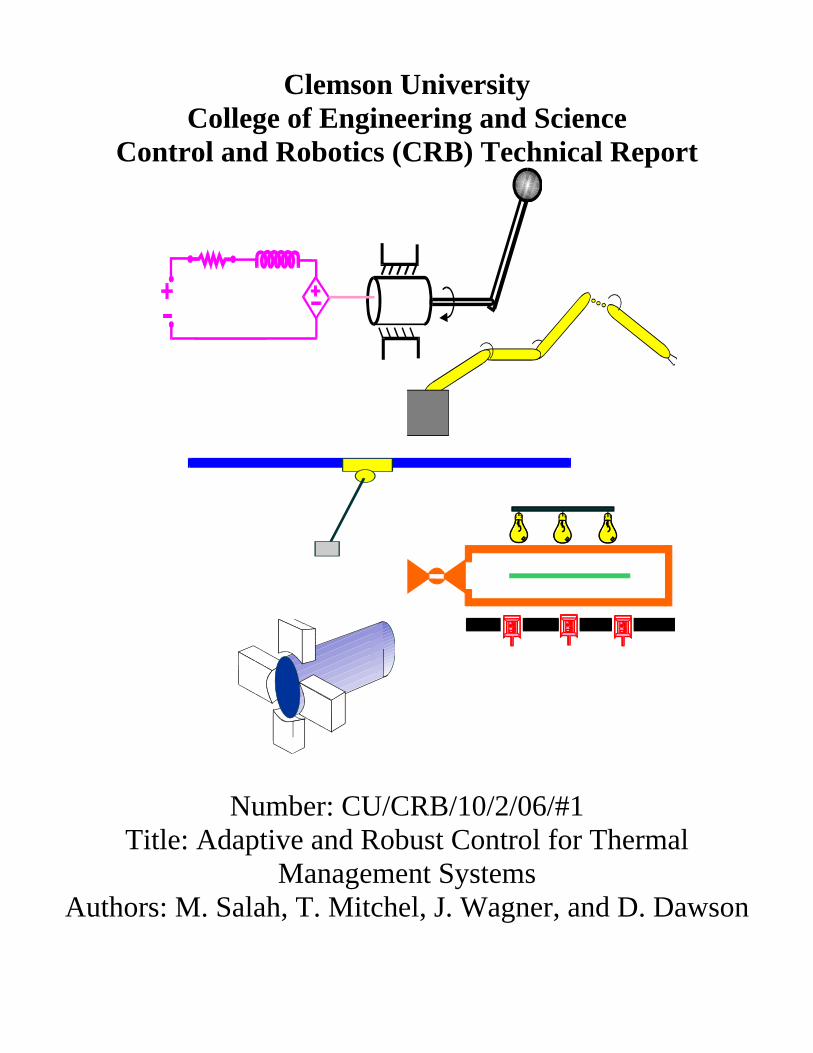
Clemson University College of Engineering and Science

Control and Robotics (CRB) Technical Report

Number: CU/CRB/10/2/06/#1 Title: Adaptive and Robust Control for Thermal

Management Systems Authors: M. Salah, T. Mitchel, J. Wagner, and D. Dawson

Report Documentation Page Form ApprovedOMB No. 0704-0188

Public reporting burden for the collection of information is estimated to average 1 hour per response, including the time for reviewing instructions, searching existing data sources, gathering andmaintaining the data needed, and completing and reviewing the collection of information. Send comments regarding this burden estimate or any other aspect of this collection of information,including suggestions for reducing this burden, to Washington Headquarters Services, Directorate for Information Operations and Reports, 1215 Jefferson Davis Highway, Suite 1204, ArlingtonVA 22202-4302. Respondents should be aware that notwithstanding any other provision of law, no person shall be subject to a penalty for failing to comply with a collection of information if itdoes not display a currently valid OMB control number.

1. REPORT DATE 2006 2. REPORT TYPE

3. DATES COVERED 00-00-2006 to 00-00-2006

4. TITLE AND SUBTITLE Adaptive and Robust Control for Thermal Management Systems

5a. CONTRACT NUMBER

5b. GRANT NUMBER

5c. PROGRAM ELEMENT NUMBER

6. AUTHOR(S) 5d. PROJECT NUMBER

5e. TASK NUMBER

5f. WORK UNIT NUMBER

7. PERFORMING ORGANIZATION NAME(S) AND ADDRESS(ES) Clemson University,Automotice Research Laboratory,Departments ofMechanical and Electrical Engineering,Clemson,SC,29634-0921

8. PERFORMING ORGANIZATIONREPORT NUMBER

9. SPONSORING/MONITORING AGENCY NAME(S) AND ADDRESS(ES) 10. SPONSOR/MONITOR’S ACRONYM(S)

11. SPONSOR/MONITOR’S REPORT NUMBER(S)

12. DISTRIBUTION/AVAILABILITY STATEMENT Approved for public release; distribution unlimited

13. SUPPLEMENTARY NOTES The original document contains color images.

14. ABSTRACT

15. SUBJECT TERMS

16. SECURITY CLASSIFICATION OF: 17. LIMITATION OF ABSTRACT

18. NUMBEROF PAGES

15

19a. NAME OFRESPONSIBLE PERSON

a. REPORT unclassified

b. ABSTRACT unclassified

c. THIS PAGE unclassified

Standard Form 298 (Rev. 8-98) Prescribed by ANSI Std Z39-18

Adaptive and Robust Control for Thermal Management Systems

M. H. Salah†, T. H. Mitchell‡, Dr. J. R. Wagner‡ P.E., and Dr. D. M. Dawson† P.E.

Automotive Research Laboratory Departments of Mechanical‡ and Electrical† Engineering

Clemson University, Clemson, SC 29634-0921 (864) 656-7376, jwagner@clemson.edu

ABSTRACT Advanced thermal management systems for internal combustion engines can improve coolant temperature regulation and servomotor power consumption by better regulating the combustion process with multiple electro-mechanical components. The traditional thermostat valve, coolant pump and clutch-driven radiator fan are upgraded with servomotor actuators. When the system components function harmoniously, desired thermal conditions can be accomplished in a power efficient manner. In this paper, a comprehensive control architecture is proposed for transient temperature tracking. An experimental system has been fabricated and assembled which features a variable position smart thermostat valve, variable speed electric water pump, variable speed electric radiator fan, engine block, and various sensors. In the configured system, the steam-based heat exchanger emulates the heat generated by the engine’s combustion process. Representative numerical and experimental results are discussed to demonstrate the functionality of the thermal management system in tracking prescribed temperature profiles.

1. INTRODUCTION Internal combustion engine active thermal management systems offer enhanced coolant temperature tracking control during transient and steady-state operation. Although the conventional automotive cooling system has proven satisfactory for many decades, servo-motor controlled cooling components have the potential to reduce the fuel consumption, parasitic losses, and tailpipe emissions (Brace et al., 2001). Advanced automotive cooling systems replace the conventional wax thermostat valve with a controllable position smart valve, and replace the mechanical water pump and radiator fan with electric and/or hydraulic driven actuators (Choukroun and Chanfreau, 2001). This replacement decouples the water pump and radiator fan from the engine crankshaft, and this solves the problem of having over/under cooling, due to the mechanical coupling, and parasitic losses associated with running mechanical components at high rotational speeds that increase exponentially (Chalgren and Barron, 2003). An assessment of thermal management strategies for large on-highway trucks and high-efficiency vehicles were described by Wambsganss (1999). Chanfreau et al. (2001) studied the benefits of engine cooling with fuel economy and emissions over the FTP drive cycle on a dual voltage 42V-12V minivan. Cho et al. (2004) investigated a controllable electric water pump in a class-3 medium duty diesel engine trucks. It was shown that the radiator size can be reduced by replacing the mechanical pump with an electrical one. Chalgren and Allen (2005) and Chalgren and Traczyk (2005) improved the temperature control, while decreasing parasitic losses, by replacing the conventional cooling system of a light duty diesel truck with an electric cooling system. To create an efficient automotive thermal management system, the vehicle’s cooling system behavior and transient response must be analyzed. Wagner et al. (2001, 2002, 2003) pursued a lumped parameter modeling approach and presented multi-node thermal models which estimate internal engine temperature. Eberth et al. (2004) presented a mathematical model to analytically predict the dynamic behavior of a 4.6L spark ignition engine. To accompany the mathematical models, analytical/empirical descriptions were developed to describe the smart cooling system components. Henry et al. (2001) developed a simulation model of powertrain cooling systems for ground vehicles. The model was validated against test results which featured basic system components (e.g., radiator, water pump, surge (return) tank, hoses and pipes, and engine thermal load). A multiple node lumped parameter-based thermal network with a suite of mathematical models, describing controllable electromechanical actuators, was introduced by Setlur et al. (2005). The proposed simplified cooling system used immersion DC heaters to emulate the engine’s combustion process and control components, with nonlinear control algorithms, to regulate the temperature. In their experiments, the water pump and radiator fan were

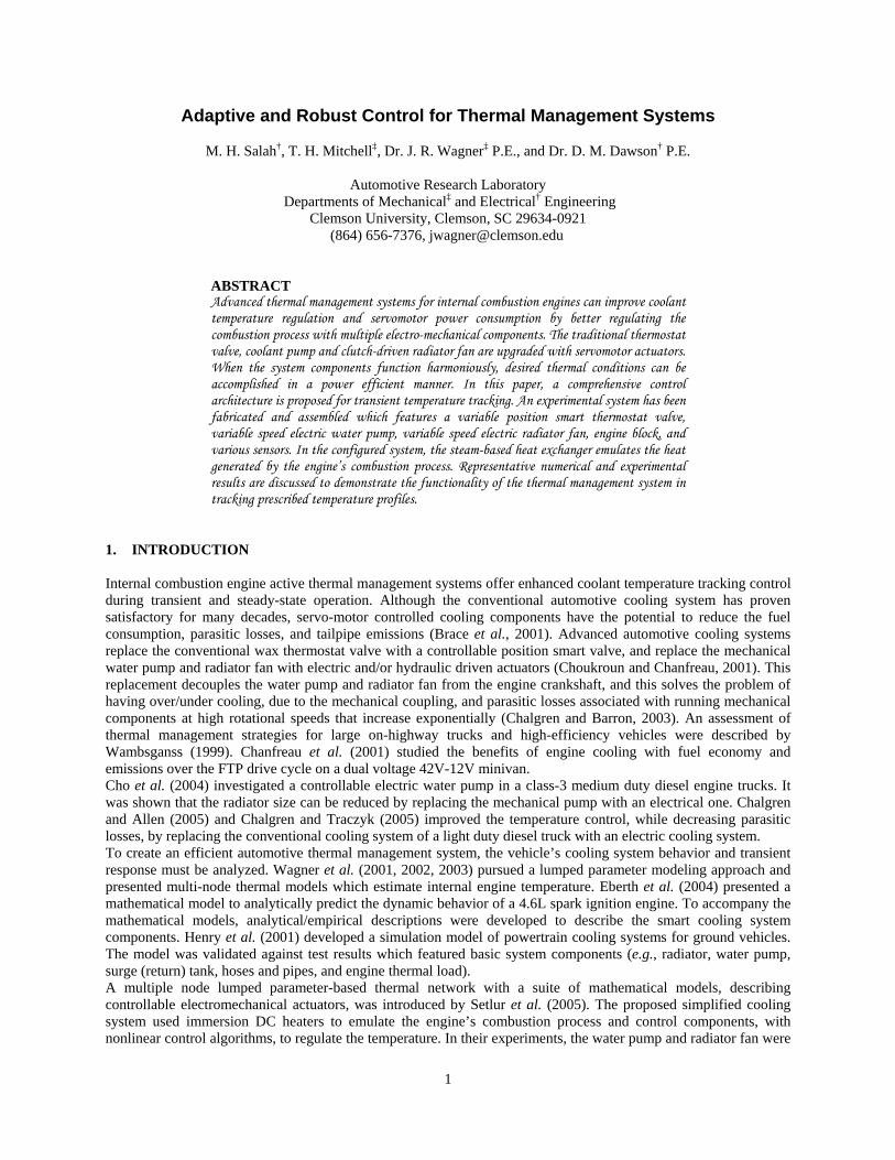
1

set to run at constant speeds, while the smart valve was controlled to trade coolant temperature set point. Cipollone and Villante (2004) tested three cooling control schemes (e.g., closed-loop, model-based, and mixed) and compared them against a traditional “thermostat-based” controller. Page et al. (2005) conducted experimental tests on a medium-sized tactical vehicle that was equipped with an intelligent thermal management system. The authors investigated improvements in the engine’s peak fuel consumption and thermal operating conditions. Finally, Redfield et al. (2006) operated a class 8 tractor at highway speeds to study potential energy saving and demonstrate engine cooling to with ±3ºC of set point value. In this paper, a nonlinear control strategy is presented to actively regulate the coolant temperature in internal combustion engines. An advanced thermal management system was implemented on a laboratory test bench that features a smart thermostat valve, variable speed electric water pump and fan, radiator, engine block, and a steam-based heat exchanger to emulate the combustion heating process. The proposed control strategies have been verified by simulation and validated by experimental testing. In Section 2, the cooling system model is presented to describe the thermal system dynamics. Nonlinear tracking control strategies are introduced in Section 3. Section 4 presents the experimental steam test bench while Section 5 introduces numerical results. Experimental results are introduced in Section 6. The conclusion is contained in Section 7. The Appendices present a Lyapunov-based stability analysis, which is needed for the controller’s design, as well as the Nomenclature List. 2. COOLING SYSTEM MODEL A reduced order two-node lumped parameter thermal model is used, as shown in Fig 1, to represent the transient response of the advanced cooling system. The system components are a 4.6L engine block, a radiator block with a variable speed electric fan, a variable position three-way smart valve, a variable speed electric water pump, and a steam-based heat exchanger to emulate the heat generated by the combustion process.

Fig 1 Advanced cooling system which features a smart valve, variable speed pump, variable speed fan, engine block, radiator, and sensors (temperature, mass flow rate, and power)

This simplified model is used to reduce the computational burden for in-vehicle implementation. The dynamics of the engine and radiator blocks at the selected nodes, as shown in Fig 1, can be described by the following differential equations

( )rerpcinee TTmCQTC −−= (1)

( ) ( )r r pc r e r o pa f eC T C m T T Q C m T Tε ∞= − − + − . (2) Because a three-way valve is used in the system, the variable is defined as , where the variable

satisfies the condition . Note that)(tmr cr mHm =

)(tH 1)(0 ≤≤ tH )0(1)( =tH corresponds to a fully closed (open) valve position and coolant flow through the bypass (radiator) loop. To facilitate the controller design process, four assumptions are imposed.

Assumption 1: The system parameters; pcC , paC , , and eC rC ε are assumed to be constants and fully known.

2

Assumption 2: It is assumed that the engine block and radiator block temperatures satisfy 0,)()( 2 ≥∀≥− ttTtT re ε where is a constant. Further we assume that to facilitate the

boundedness of signal argument.

+ℜ∈2ε )0()0( re TT ≥

Assumption 3: It is assumed that the surrounding ambient temperature is constant and satisfies )(tT∞0,)()( 1 ≥∀≥− ∞ ttTtTr ε where is a constant. +ℜ∈1ε

Assumption 4: From the problem physics, the signals and always remain positive in (1), and (2) (i.e. ).

)(tQin )(tQo0)(),( ≥tQtQ oin

3. THERMAL CONTROL SYSTEM DESIGNS In this paper, two Lyapunov-based nonlinear control algorithms are presented to maintain a desired thermal condition for the engine block. The objective of the proposed control strategies is to get a precise engine temperature tracking while compensating for the system uncertainties (e.g. combustion process heat input and external ram air disturbance) by harmoniously controlling the system actuators. The control objective of the nonlinear control strategies is to ensure that the actual temperatures of the engine block

and the radiator block track the desired trajectories and , respectively, in the following sense

)(tTe )(tTr )(tTed )(tTrd

( ) ( )e edT t T t→ as ∞→t , as ( ) ( )r rdT t T t→ ∞→t (3) while compensating for the system uncertainties and . )(tQin )(tQo

Remark 1: It is assumed that the desired engine and radiator temperature profiles are selected such that they are always bounded and their first three time derivatives remain bounded at all times (i.e.,

. Further more, at all times. ),(),(),(),(),(),(),( tTtTtTtTtTtTtT rdrdrdedededed ∞∈ LtTrd )( ( ) ( )ed rdT t T t T∞>> >> 3.1 Adaptive Control Strategy To facilitate the controller’s development and quantify the temperature tracking control objective, the following signals are defined

ed ee T T− , rd rT Tη − . (4)

Assumption 5: It is assumed that the signals and are constants at all time. )(tQin )(tQo

3.1.1 Closed-Loop Error System Development and Controller Formulation

The open-loop error system can be analyzed by taking the first time derivative of both expressions in (4) and then multiplying both sides of the resulting equations by and for the engine and radiator dynamics, respectively. Thus, the system dynamics described in (1) and (2) can be substituted and then reformatted to realize

eC rC

eeedee uTCeC +−= θ , (5) rrrdrr uTCC −+= θη where ( ) ( )tQt ine =θ , ( ) ( )tQt or =θ , ( ) ( )e pc r eu t C m T T− r , and ( ) ( ) (r pc r e r pa f eu t C m T T C m T Tε )∞− − − .

Remark 2: The control inputs and ( )rm t ( )tm f are uni-polar. Hence, commutation strategies are designed to

implement the bi-polar inputs and ( )eu t ( )ru t as

( )( )

( )( )

1 sgn 1 sgn,

2 2e e

r fpc e r pa e

u u F Fm m

C T T C T Tε ∞

⎡ ⎤ ⎡ ⎤+ +⎣ ⎦ ⎣− −

⎦ (6)

where ( ) ( )pc r e r rF t C m T T u− − . The control input, ( )tm f is obtained from (6) after is computed. From

these definitions, it is clear that if ( )rm t

( ) ( ), 0e ru t u t L t∞∈ ∀ ≥ , then ( ) ( ),r fm t m t L t∞ 0∈ ∀ ≥ . From the calculation of

3

the radiator mass flow rate and using a three-way valve in the system, the water pump speed can be determined for a given valve position or the valve position can be determined for a given water pump speed.

( )rm t

To satisfy the control objectives stated earlier, continuous control laws ( )tue and ( )tur can be designed as follows

eKTCu eedeee −−= θ̂ , (7) ηθ rrdrrr KTCu ++= ˆ

where the estimates and are to compensate for the system constants uncertainties and , and designed as follows

( )teθ̂ ( )trθ̂ )(tQin )(tQo

( ) τταθ det

teeo∫−=ˆ , (8) ( ) ττηαθ d

t

trro∫=ˆ

3.1.2 Stability Analysis

Theorem 1: The controller given in (7) ensures asymptotic engine and radiator temperatures tracking (i.e. ( ) ( ) 0, →tte η as ∞→t ) and all closed-loop signals are bounded.

Proof: See Appendix A for the complete Lyapunov-based stability analysis. 3.2 Robust Control Strategy

To facilitate the controllers’ development and quantify the temperature tracking control objective, a filtered tracking error is defined as follows

e es e eα+ , r rs η α η+ (9) where and )(te )(tη were defined in (4).

Assumption 6: It is assumed that the signals and vary with time and their first two time

derivatives remain bounded at all time, such that .

)(tQin )(tQo

∞∈ LtQtQtQtQtQtQ oooininin )(),(),(),(),(),( 3.2.1 Closed-Loop Error System Development and Controller Formulation The open-loop error system can be analyzed by taking the first time derivative of both expressions in (9) and then multiplying both sides of the resulting equations by and for the engine and radiator dynamics, respectively. Thus, the system dynamics described in (1) and (2) can be substituted and then reformatted to realize

eC rC

eCuQTCsC eeeinedeee α++−= , (10) ηα rrrordrrr CuQTCsC +−+=

where (4) and it is first time derivative were utilized provided the signals ( )eu t and are defined as

and ( )ru t

( ) ( )e pc r eu t C m T T− r ( ) ( ) ( )r pc r e r pa f ru t C m T T C m T Tε ∞− − − .

Remark 3: The control inputs and ( )rm t ( )tm f are uni-polar. Hence, the commutation strategies, designed in

(6), are used to implement the bi-polar inputs ( )eu t and ( )ru t .

To facilitate the subsequent analysis, the expressions in (10) are rewritten as follows

euNNsC eedeee −++=~ , r r r rd rC s N N u η= + − − (11)

where the auxiliary signals ( )tTTN eee ,,~ and ( )tTTN rrr ,,~ are defined as follows

edee NNN −=~ , rdrr NNN −=

~ (12)

4

where and are defined as follows ( )tTTN eee ,, ( tTTN rrr ,, )

e

e e ed in e eN C T Q C eα− + + , r r rd o r rN C T Q C α η η+ + + (13) and both and are defined as follows ( )tNed ( )tNrd

,e ed e eded e e ed inT T T TN N C T Q= =≡ = − , ,r rd r rdrd r r rd oT T T TN N C T Q= =≡ = + . (14)

Based on (12) through (14), the control laws introduced in (11) are designed as follows

( )[ ] ( )[ ] ττρτααα deeKeeKut

t eeeeoeeeo∫ ++−−+−= ))(sgn()( (15)

( ) ( ) ( ) sgn( ( ))o

tr r r o r r r rt

u K K dα η η α α η τ ρ η τ τ⎡ ⎤= + − + + +⎡ ⎤⎣ ⎦ ⎣ ⎦∫ (16)

where ooe η, are ( ) ( )tte η, , respectively, computed at the initial time . The terms and ot oe oη in (15) and (16), respectively, are included so that and equal to zero, where the “sgn” terms compensate for the unknown quantities in (13). The time derivatives of (15) and (16) are given by the following expressions

)( oe tu )( oe tu

( ) )sgn(esKu eeeee ρα −+−= , ( ) sgn( )r r r r ru K sα ρ η= + + . (17)

After substituting (17) into (11), the closed-loop error system can be obtained as follows

( ) eesKNNsC eeeeedeee −−+−+= )sgn(~ ρα (18)

( ) ηηρα −−+−+= )sgn(~rrrrrdrrr sKNNsC . (19)

Remark 4: Based on Remark 1, Assumption 6, and the expressions in (14), ( ) ( ) ( )tNtNtN rdeded ,, and ( )tNrd

can be upper bounded by known positive constants as follows

1ed eN ζ≤ , 2ed eN ζ≤ , 1rd rN ζ≤ , 2rd rN ζ≤ . (20)

3.2.2 Stability Analysis

Theorem 2: The controller given in (15) and (16) ensures asymptotic engine and radiator temperatures tracking (i.e. ( ) ( ) ( ) ( ) 0,,, →tsttste re η as ∞→t ) and all closed-loop signals are bounded provided the control gains eρ and

rρ are selected to satisfy the following sufficient conditions

211

ee

ee ζα

ζρ +> , 211

rr

rr ζα

ζρ +> (21)

where 121 ,, ree ζζζ and 2rζ are given in (20), and and are selected sufficiently large. eK rKProof: See Appendix B for the complete Lyapunov-based stability analysis.

4. STEAM TEST BENCH

An experimental test bench (refer to Figure 2) has been fabricated to demonstrate the proposed advanced thermal management system controller design. The assembled test bench offers a flexible, rapid, repeatable, and safe testing environment. Clemson University facilities generated steam is utilized to rapidly heat the coolant circulating within the cooling system via a two-pass shell and tube heat exchanger. The heated coolant is then routed through a 6.0L diesel engine block to emulate the combustion process heat. From the engine block, the coolant flows to a three-way smart valve and then either through the bypass or radiator to the water pump to close the loop. The thermal response

5

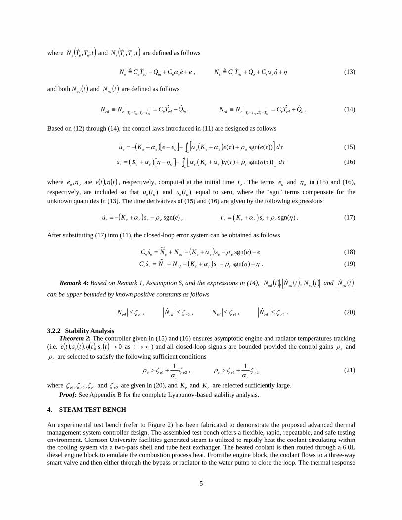
of the engine block to the adjustable, externally applied heat source emulates the heat transfer process between the combustion gases, cylinder wall, and water jacket in an actual operating engine. As shown in Figure 1, the system sensors include three type-J thermocouples (e.g., T1 = engine temperature, T2 = radiator temperature, and T3 = ambient temperature), two mass flow meters (e.g., M1 = coolant mass flow meter, and M2 = air mass flow meter), and electric voltage and current measurements (e.g., P1 = valve power consumed, P2 = pump power consumed, and P3 = fan power consumed).

Fig 2 Experimental thermal test bench that features a 6.0L diesel engine block, three-way smart valve, electric water pump, electric radiator fan, radiator, and steam-based heat exchanger The steam bench can provide up to 55 kW of energy. High pressure saturated steam (412 kPa) is routed from the campus facilities plant to the steam test bench, where a pressure regulator reduces the steam pressure to 172 kPa before it enters the low pressure filter. The low pressure saturated steam is then routed to the double pass steam heat exchanger to heat the system’s coolant. The amount of energy transferred to the system is controlled by the main valve mounted on the heat exchanger. The mass flow rate of condensate is proportional to the energy transfer to the circulating coolant. Condensed steam may be collected and measured to calculate the rate of energy transfer. From steam tables, the enthalpy of condensation can be acquired. To facilitate the analysis, pure saturated steam and condensate at approximately T=100ºC determines the enthalpy of condensation. Baseline testing was performed to determine the average energy transferred to the coolant at various steam control valve positions. The coolant temperatures were initialized at Te = 67ºC before measuring the condensate. Each test was executed for different time periods.

5. SIMULATION RESULTS 5.1 Adaptive Control Test 1: Constant Heat Input and External Disturbance A numerical simulation for the adaptive control strategy, introduced in Section 3.1, has been performed on the system dynamics described in (1) and (2) to demonstrate the performance of the proposed controller given in (7) and (8). The simulated thermal system’s parameters were set to the following: [J/ºK],

[J/kg.ºK], [J/kg.ºK], 63250CC re ==

4186=pcC 1000=paC 6.0=ε , ( ) 300=∞ tT [ºK], ( ) 8214.0=tmc [kg/sec], ( ) 30=tQin [kW] and [kW]. The initial simulation conditions were set to be as follows: [ºK] and

[ºK]. The desired temperatures were selected to be ( ) 7=tQo ( ) 3600 =eT

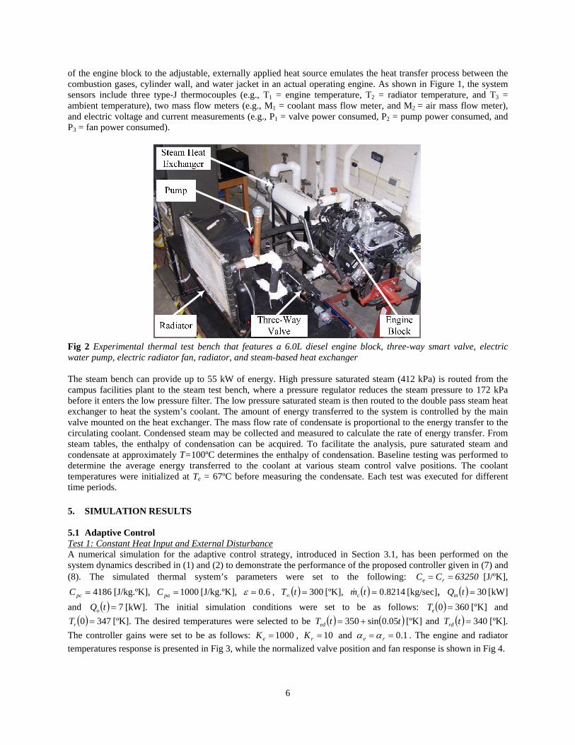
( ) 3470 =rT ( ) ( )ttTed 05.0sin350 += [ºK] and ( ) 340=tTrd [ºK]. The controller gains were set to be as follows: 1000=eK , 10=rK and 1.0== re αα . The engine and radiator temperatures response is presented in Fig 3, while the normalized valve position and fan response is shown in Fig 4.

6

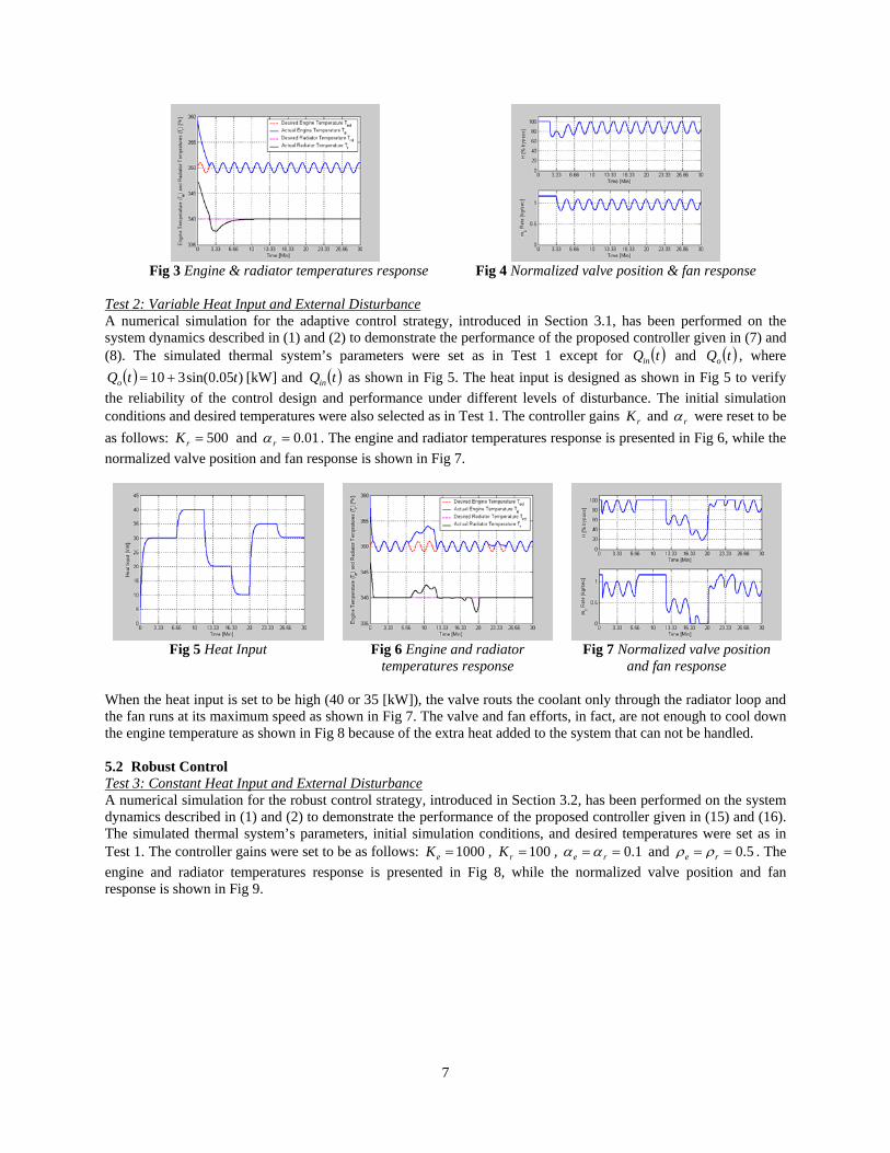
Fig 3 Engine & radiator temperatures response

Fig 4 Normalized valve position & fan response

Test 2: Variable Heat Input and External Disturbance A numerical simulation for the adaptive control strategy, introduced in Section 3.1, has been performed on the system dynamics described in (1) and (2) to demonstrate the performance of the proposed controller given in (7) and (8). The simulated thermal system’s parameters were set as in Test 1 except for and ( )tQin ( )tQo , where

[kW] and as shown in Fig 5. The heat input is designed as shown in Fig 5 to verify the reliability of the control design and performance under different levels of disturbance. The initial simulation conditions and desired temperatures were also selected as in Test 1. The controller gains and

( ) )05.0sin(310 ttQo += ( )tQin

rK rα were reset to be as follows: and 500=rK 01.0=rα . The engine and radiator temperatures response is presented in Fig 6, while the normalized valve position and fan response is shown in Fig 7.

Fig 5 Heat Input Fig 6 Engine and radiator

temperatures response Fig 7 Normalized valve position

and fan response When the heat input is set to be high (40 or 35 [kW]), the valve routs the coolant only through the radiator loop and the fan runs at its maximum speed as shown in Fig 7. The valve and fan efforts, in fact, are not enough to cool down the engine temperature as shown in Fig 8 because of the extra heat added to the system that can not be handled. 5.2 Robust Control Test 3: Constant Heat Input and External Disturbance A numerical simulation for the robust control strategy, introduced in Section 3.2, has been performed on the system dynamics described in (1) and (2) to demonstrate the performance of the proposed controller given in (15) and (16). The simulated thermal system’s parameters, initial simulation conditions, and desired temperatures were set as in Test 1. The controller gains were set to be as follows: 1000=eK , 100=rK , 1.0== re αα and 5.0== re ρρ . The engine and radiator temperatures response is presented in Fig 8, while the normalized valve position and fan response is shown in Fig 9.

7

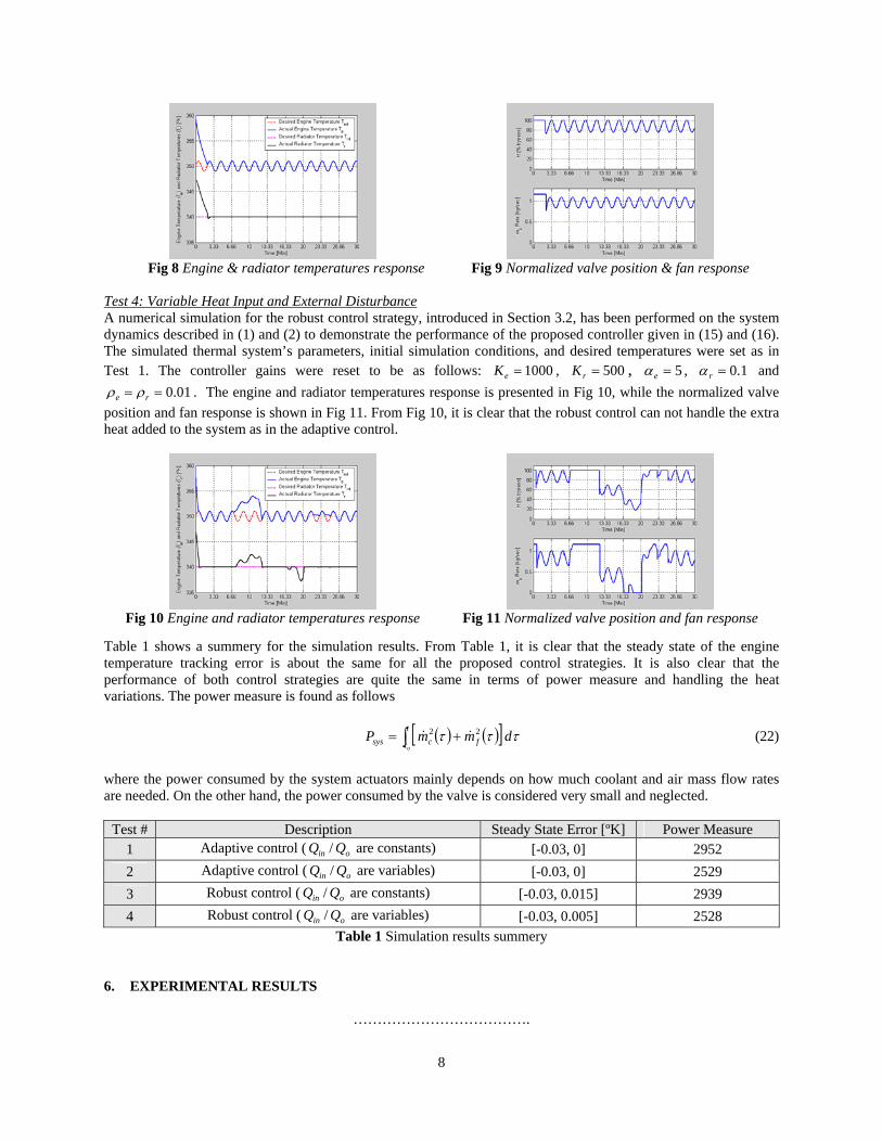
Fig 8 Engine & radiator temperatures response

Fig 9 Normalized valve position & fan response

Test 4: Variable Heat Input and External Disturbance A numerical simulation for the robust control strategy, introduced in Section 3.2, has been performed on the system dynamics described in (1) and (2) to demonstrate the performance of the proposed controller given in (15) and (16). The simulated thermal system’s parameters, initial simulation conditions, and desired temperatures were set as in Test 1. The controller gains were reset to be as follows: 1000=eK , 500=rK , 5=eα , 1.0=rα and

01.0== re ρρ . The engine and radiator temperatures response is presented in Fig 10, while the normalized valve position and fan response is shown in Fig 11. From Fig 10, it is clear that the robust control can not handle the extra heat added to the system as in the adaptive control.

Fig 10 Engine and radiator temperatures response Fig 11 Normalized valve position and fan response

Table 1 shows a summery for the simulation results. From Table 1, it is clear that the steady state of the engine temperature tracking error is about the same for all the proposed control strategies. It is also clear that the performance of both control strategies are quite the same in terms of power measure and handling the heat variations. The power measure is found as follows

( ) ( )[ ] τττ dmmPt

t fcsyso∫ += 22 (22)

where the power consumed by the system actuators mainly depends on how much coolant and air mass flow rates are needed. On the other hand, the power consumed by the valve is considered very small and neglected.

Test # Description Steady State Error [ºK] Power Measure 1 Adaptive control ( are constants) oin QQ / [-0.03, 0] 2952 2 Adaptive control ( are variables) oin QQ / [-0.03, 0] 2529 3 Robust control ( are constants) oin QQ / [-0.03, 0.015] 2939 4 Robust control ( are variables) oin QQ / [-0.03, 0.005] 2528

Table 1 Simulation results summery 6. EXPERIMENTAL RESULTS

……………………………….

8

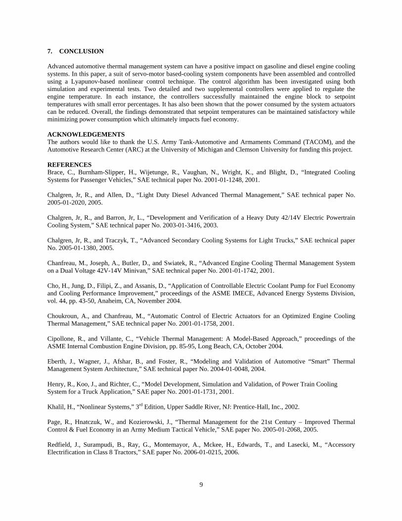
7. CONCLUSION

Advanced automotive thermal management system can have a positive impact on gasoline and diesel engine cooling systems. In this paper, a suit of servo-motor based-cooling system components have been assembled and controlled using a Lyapunov-based nonlinear control technique. The control algorithm has been investigated using both simulation and experimental tests. Two detailed and two supplemental controllers were applied to regulate the engine temperature. In each instance, the controllers successfully maintained the engine block to setpoint temperatures with small error percentages. It has also been shown that the power consumed by the system actuators can be reduced. Overall, the findings demonstrated that setpoint temperatures can be maintained satisfactory while minimizing power consumption which ultimately impacts fuel economy. ACKNOWLEDGEMENTS The authors would like to thank the U.S. Army Tank-Automotive and Armaments Command (TACOM), and the Automotive Research Center (ARC) at the University of Michigan and Clemson University for funding this project. REFERENCES Brace, C., Burnham-Slipper, H., Wijetunge, R., Vaughan, N., Wright, K., and Blight, D., “Integrated Cooling Systems for Passenger Vehicles,” SAE technical paper No. 2001-01-1248, 2001. Chalgren, Jr, R., and Allen, D., “Light Duty Diesel Advanced Thermal Management,” SAE technical paper No. 2005-01-2020, 2005. Chalgren, Jr, R., and Barron, Jr, L., “Development and Verification of a Heavy Duty 42/14V Electric Powertrain Cooling System,” SAE technical paper No. 2003-01-3416, 2003. Chalgren, Jr, R., and Traczyk, T., “Advanced Secondary Cooling Systems for Light Trucks,” SAE technical paper No. 2005-01-1380, 2005. Chanfreau, M., Joseph, A., Butler, D., and Swiatek, R., “Advanced Engine Cooling Thermal Management System on a Dual Voltage 42V-14V Minivan,” SAE technical paper No. 2001-01-1742, 2001. Cho, H., Jung, D., Filipi, Z., and Assanis, D., “Application of Controllable Electric Coolant Pump for Fuel Economy and Cooling Performance Improvement,” proceedings of the ASME IMECE, Advanced Energy Systems Division, vol. 44, pp. 43-50, Anaheim, CA, November 2004. Choukroun, A., and Chanfreau, M., “Automatic Control of Electric Actuators for an Optimized Engine Cooling Thermal Management,” SAE technical paper No. 2001-01-1758, 2001. Cipollone, R., and Villante, C., “Vehicle Thermal Management: A Model-Based Approach,” proceedings of the ASME Internal Combustion Engine Division, pp. 85-95, Long Beach, CA, October 2004. Eberth, J., Wagner, J., Afshar, B., and Foster, R., “Modeling and Validation of Automotive “Smart” Thermal Management System Architecture,” SAE technical paper No. 2004-01-0048, 2004. Henry, R., Koo, J., and Richter, C., “Model Development, Simulation and Validation, of Power Train Cooling System for a Truck Application,” SAE paper No. 2001-01-1731, 2001. Khalil, H., “Nonlinear Systems,” 3rd Edition, Upper Saddle River, NJ: Prentice-Hall, Inc., 2002. Page, R., Hnatczuk, W., and Kozierowski, J., “Thermal Management for the 21st Century – Improved Thermal Control & Fuel Economy in an Army Medium Tactical Vehicle,” SAE paper No. 2005-01-2068, 2005. Redfield, J., Surampudi, B., Ray, G., Montemayor, A., Mckee, H., Edwards, T., and Lasecki, M., “Accessory Electrification in Class 8 Tractors,” SAE paper No. 2006-01-0215, 2006.

9

Setlur, P., Wagner, J., Dawson, D., and Marotta, E., “An Advanced Engine Thermal Management System: Nonlinear Control and Test”, IEEE/ASME Transactions on Mechatronics, vol. 10, no. 2, pp. 210-220, April 2005. Wagner, J., Marotta, E., and Paradis, I., “Thermal Modeling of Engine Components for Temperature Prediction and Fluid Flow Regulation”, SAE technical paper No. 2001-01-1014, 2001. Wagner, J., Ghone, M., Dawson, D., and Marotta, E., “Coolant Flow Control Strategies for Automotive Thermal Management Systems,” SAE technical paper No. 2002-01-0713, 2002. Wagner, J., Srinivasan, V., and Dawson, D., “Smart Thermostat and Coolant Pump Control for Engine Thermal Management Systems,” SAE technical paper No. 2003-01-0272, 2003. Wambsganss, M., “Thermal Management Concepts for Higher-Efficiency Heavy Vehicle,” SAE technical paper No. 1999-01-2240, 1999.

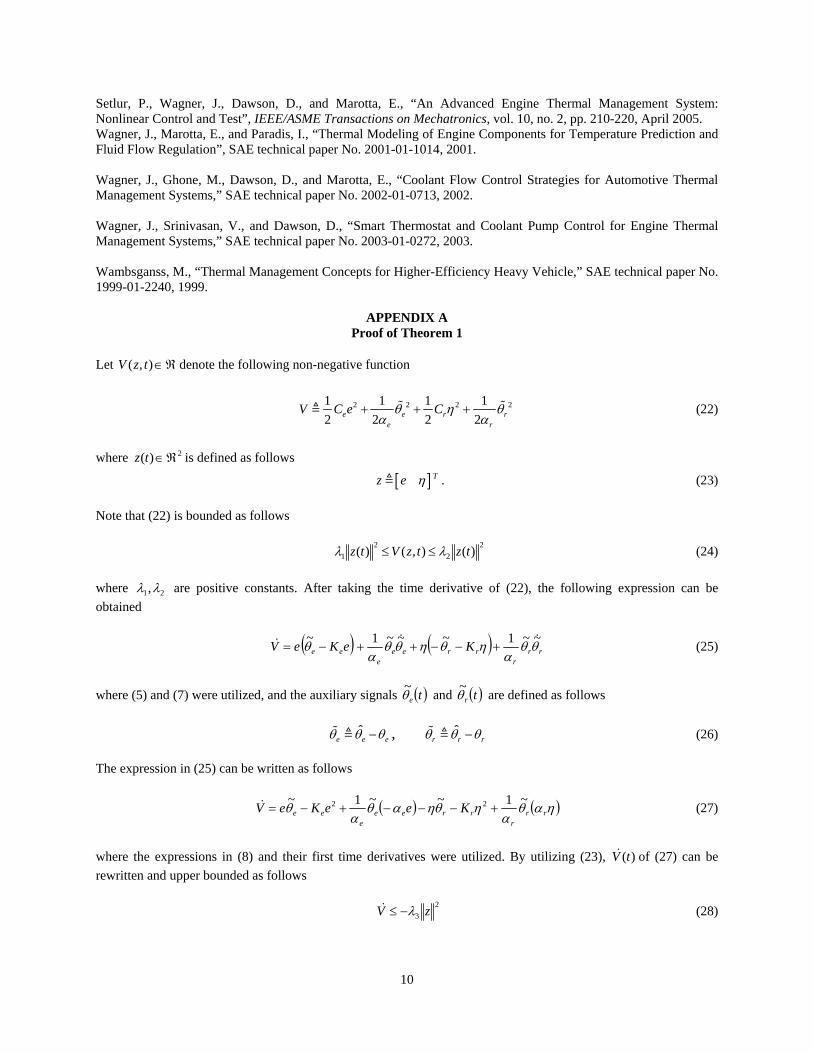
APPENDIX A Proof of Theorem 1

Let denote the following non-negative function ℜ∈),( tzV

2 2 21 1 1 12 2 2 2e e r

e r

V C e C 2rθ η θ

α α+ + + (22)

where is defined as follows 2)( ℜ∈tz

[ ] Tz e η . (23) Note that (22) is bounded as follows

22

21 )(),()( tztzVtz λλ ≤≤ (24)

where 21,λλ are positive constants. After taking the time derivative of (22), the following expression can be obtained

( ) ( ) rrr

rreee

ee KeKeV θθα

ηθηθθα

θ~~1~~~1~

+−−++−= (25)

where (5) and (7) were utilized, and the auxiliary signals ( )teθ

~ and ( )trθ~ are defined as follows

ˆ

e e eθ θ θ− , ˆr r rθ θ θ− (26)

The expression in (25) can be written as follows

( ) ( )ηαθα

ηθηαθα

θ rrr

rreee

ee KeeKeV ~1~~1~ 22 +−−−+−= (27)

where the expressions in (8) and their first time derivatives were utilized. By utilizing (23), of (27) can be rewritten and upper bounded as follows

)(tV

2

3 zV λ−≤ (28)

10

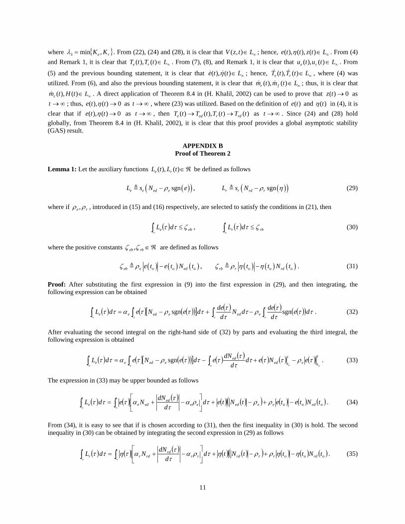
where { re KK ,min3 = }λ . From (22), (24) and (28), it is clear that ∞∈ LtzV ),( ; hence, ∞∈ Ltztte )(),(),( η . From (4) and Remark 1, it is clear that . From (7), (8), and Remark 1, it is clear that ∞∈ LtTtT re )(),( ∞∈ Ltutu re )(),( . From

(5) and the previous bounding statement, it is clear that ∞∈ Ltte )(),( η ; hence, , where (4) was utilized. From (6), and also the previous bounding statement, it is clear that ; thus, it is clear that

. A direct application of Theorem 8.4 in (H. Khalil, 2002) can be used to prove that as

∞∈ LtTtT re )(),(( ), ( )r fm t m t L∞∈

∞∈ LtHtmc )(),( 0)( →tz∞→t ; thus, 0)(),( →tte η as ∞→t , where (23) was utilized. Based on the definition of and )(te )(tη in (4), it is

clear that if 0)(),( →tte η as ∞→t , then as )()(),()( tTtTtTtT rdrede →→ ∞→t . Since (24) and (28) hold globally, from Theorem 8.4 in (H. Khalil, 2002), it is clear that this proof provides a global asymptotic stability (GAS) result.

APPENDIX B Proof of Theorem 2

Lemma 1: Let the auxiliary functions ℜ∈)(),( tLtL re be defined as follows

( )( )sgne e ed eL s N eρ− , ( )( )sgnr r rd rL s N ρ η− (29) where if re ρρ , , introduced in (15) and (16) respectively, are selected to satisfy the conditions in (21), then

( ) ebt

t eo

dL ζττ ≤∫ , (30) ( ) rbt

t ro

dL ζττ ≤∫ where the positive constants ℜ∈rbeb ζζ , are defined as follows

( ) ( ) ( )eb e o o ed oe t e t N tζ ρ − , ( ) ( ) (rb r o o rd ot t N tζ ρ η η− ) . (31) Proof: After substituting the first expression in (9) into the first expression in (29), and then integrating, the following expression can be obtained

( ) ( ) ( )( )[ ] ( ) ( ) ( )( ) ττττρτ

ττττρταττ de

ddedN

ddedeNedL

t

t

t

t eedt

t eedet

t eoooo∫∫∫∫ −+−= sgnsgn . (32)

After evaluating the second integral on the right-hand side of (32) by parts and evaluating the third integral, the following expression is obtained

( ) ( ) ( )( )[ ] ( ) ( ) ( ) ( ) ( ) t

t

t

t et

tededt

t eedet

t eoo ooo

eNedd

dNedeNedL τρττττττττρταττ ∫∫∫ −+−−= sgn . (33)

The expression in (33) may be upper bounded as follows

( ) ( ) ( ) ( ) ( )( ) ( ) ( ) ( )oedooeeedt

t eeed

edet

t e tNtetetNtedd

dNNedLoo

−+−+⎥⎦

⎤⎢⎣

⎡−+= ∫∫ ρρτρα

ττατττ . (34)

From (34), it is easy to see that if is chosen according to (31), then the first inequality in (30) is hold. The second inequality in (30) can be obtained by integrating the second expression in (29) as follows

( ) ( ) ( ) ( ) ( )( ) ( ) ( ) ( )ordoorrrdt

t rrrd

rdrt

t r tNtttNtdd

dNNdLoo

ηηρρητραττατηττ −+−+⎥

⎦

⎤⎢⎣

⎡−+= ∫∫ . (35)

11

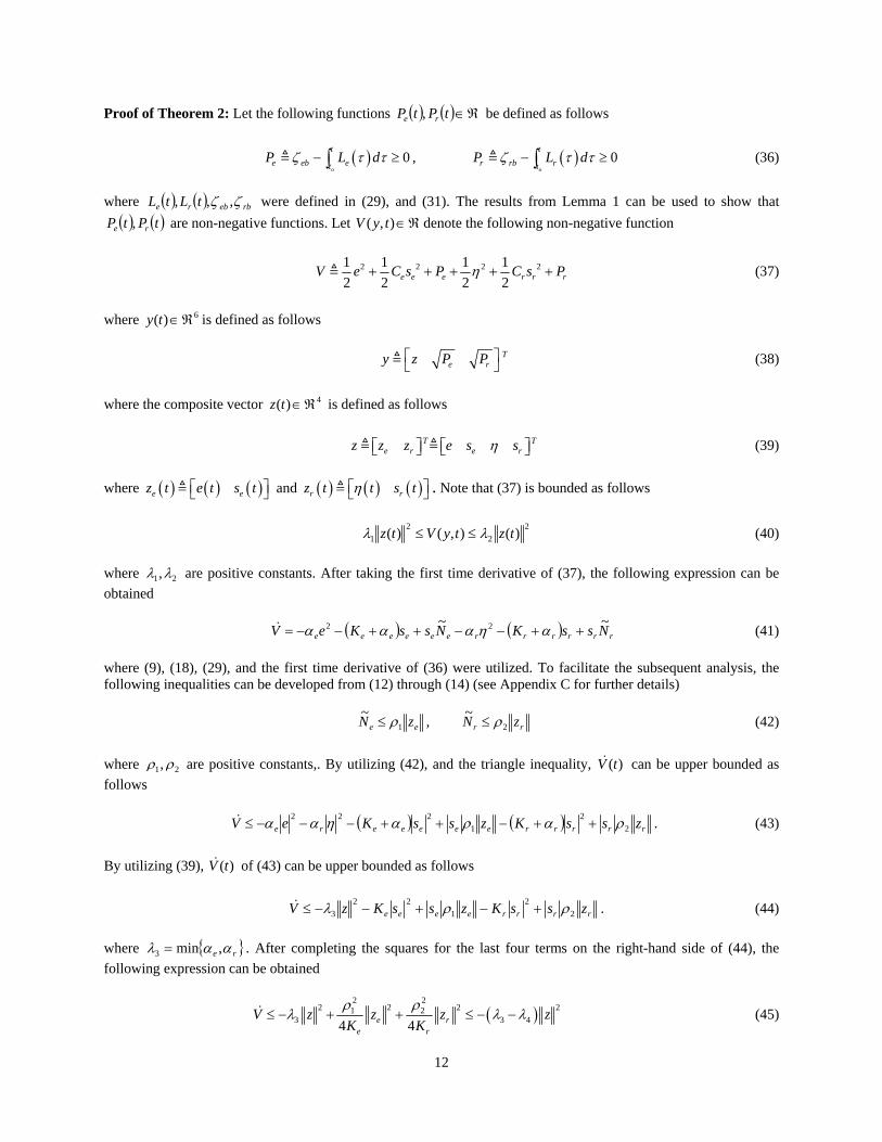
Proof of Theorem 2: Let the following functions ( ) ( ) ℜ∈tPtP re , be defined as follows

( ) 0o

te eb et

P L dζ τ τ− ≥∫ , ( ) 0o

tr rb rt

P L dζ τ τ− ≥∫ (36)

where ( ) ( ) rbebre tLtL ζζ ,,, were defined in (29), and (31). The results from Lemma 1 can be used to show that

are non-negative functions. Let ( ) ( )tPtP re , ℜ∈),( tyV denote the following non-negative function

2 2 2 21 1 1 12 2 2 2e e e r r rV e C s P C sη P+ + + + + (37)

where is defined as follows 6)( ℜ∈ty

Te ry z P P⎡ ⎤

⎣ ⎦ (38)

where the composite vector is defined as follows 4)( ℜ∈tz

T Te r e rz z z e s sη⎡ ⎤ ⎡ ⎤⎣ ⎦ ⎣ ⎦ (39)

where and ( ) ( ) ( )e ez t e t s t⎡ ⎤⎣ ⎦ ( ) ( ) ( )rz t t s tη⎡⎣ r ⎤⎦ . Note that (37) is bounded as follows

22

21 )(),()( tztyVtz λλ ≤≤ (40)

where 21,λλ are positive constants. After taking the first time derivative of (37), the following expression can be obtained

( ) ( ) rrrrrreeeeee NssKNssKeV ~~ 22 ++−−++−−= αηααα (41) where (9), (18), (29), and the first time derivative of (36) were utilized. To facilitate the subsequent analysis, the following inequalities can be developed from (12) through (14) (see Appendix C for further details)

ee zN 1~ ρ≤ , rr zN 2

~ ρ≤ (42) where 21,ρρ are positive constants,. By utilizing (42), and the triangle inequality, can be upper bounded as follows

)(tV

( ) ( ) rrrrreeeeere zssKzssKeV 2

21

222 ραραηαα ++−++−−−≤ . (43) By utilizing (39), of (43) can be upper bounded as follows )(tV

rrrreeee zssKzssKzV 22

122

3 ρρλ +−+−−≤ . (44) where { re }ααλ ,min3 = . After completing the squares for the last four terms on the right-hand side of (44), the following expression can be obtained

( )2 2

22 21 23 34 4e r

e r

V z z zK Kρ ρ

λ λ≤ − + + ≤ − − 24 zλ (45)

12

where ⎭⎬⎫

⎩⎨⎧

=re KK 4

,4

min22

21

4ρρλ . Provided that and are selected so that the condition eK rK 43 λλ ≥ is satisfied, then

the following inequality can be developed

)( yWV ≤ (46) where denotes the following non-negative function ℜ∈)(yW

2)( zyW γ−≤ (47) where γ denotes a positive constant. From (37), (40), (46), and (47), it is clear that ; hence, ∞∈ LtyV ),(

∞∈ Ltytztztztststte eere )(),(),(),(),(),(),(),( η . From (4), and Remark 1, it is clear that . From (9), it

is clear that ∞∈ LtTtT re )(),(

∞∈ Ltte )(),( η . Thus, from Remark 1, it is clear that . The previous bounding statement can be used along with (15) and (16) to prove that

∞∈ LtTtT re )(),(

∞∈ Ltutu re )(),( . Thus, from (6), it is clear that ( ), ( )r fm t m t L∞∈ ; hence, it is clear that . A direct application of Theorem 8.4 in (H. Khalil, 2002) can be used to prove that as

∞∈ LtHtmc )(),(0)( →tz ∞→t ; thus, ( ) ( ) 0),(,),( →tsttste re η as ∞→t , where (39) was utilized. Based on the

definition of and )(te )(tη in (4), it is clear that if 0)(),( →tte η as ∞→t , then as )()(),()( tTtTtTtT rdrede →→∞→t . Since (40), (46) and (47) hold globally, from Theorem 8.4 in (H. Khalil, 2002), it is clear that this proof

provides a global asymptotic stability (GAS) result.

APPENDIX C Upper Bound Development for Robust Control

By substituting (13) and (14) into (12), the expressions of ( )tTTN eee ,,~ and ( )tTTN rrr ,,~ can be written as follows

eeCN eee +≡ α~ , ηηα +≡ rrr CN~ (48) which may be upper bounded as follows

eeCN eee +≤ α~ , ηηα +≤ rrr CN~ . (49) Using the definition of and , given in (39), ( )tze ( )tzr ( )tTTN eee ,,~ , and ( )tTTN rrr ,,~ can be bounded as follows

ee zN 1~ ρ≤ , rr zN 2

~ ρ≤ . (50)

Appendix D NOMENCLATURE LIST

eα positive control gain

rβ positive constant [Rad/sec.m2]

eC engine block capacity [kJ/ºK]

pcC coolant specific heat [kJ/kg.ºK]

paC air specific heat [kJ/kg.ºK]

rC radiator capacity [kJ/ºK] e engine temperature tracking error [ºK]

oe initial engine temperature tracking error [ºK]

sse engine temperature steady state error [ºK] ε effectiveness of the radiator fan [%] η radiator temperature tracking error [ºK] H normalized valve position [%]

cm pump coolant mass flow rate [kg/sec]

fm fan air mass flow rate [kg/sec]

rm radiator coolant mass flow rate [kg/sec]

1M pump coolant mass flow rate meter

13

2M radiator fan air mass flow rate meter oQ radiator heat lost due to uncontrollable air flow [kW] 1P valve power sensor

sgn standard signum function 2P water pump power sensor

ot initial time [sec] 3P radiator fan power sensor

1T coolant temperature at engine outlet [ºK] MP cooling system power measure [W]

2T coolant temperature at radiator outlet [ºK] sysP cooling system power consumption [W]

3T ambient temperature sensor [ºK] vP valve power consumption [W]

eT coolant temperature at the engine outlet [ºK] eρ positive constant

∞T surrounding ambient temperature [ºK] inQ combustion process heat energy [kW]

rT radiator outlet coolant temperature [ºK]

edT desired engine temperature trajectory [ºK]

14