Click Here Full Article Modeling integrated water user ... integrated water user decisions in intermittent supply systems David E. Rosenberg,1 Tarek Tarawneh,2 Rania Abdel-Khaleq,3

Modeling integrated water user decisions

in intermittent supply systems

David E. Rosenberg,1 Tarek Tarawneh,2 Rania Abdel-Khaleq,3 and Jay R. Lund1

Received 12 July 2006; revised 20 January 2007; accepted 26 February 2007; published 17 July 2007.

[1] We apply systems analysis to estimate household water use in an intermittent supplysystem considering numerous interdependent water user behaviors. Some 39 householdactions include conservation; improving local storage or water quality; and accessingsources having variable costs, availabilities, reliabilities, and qualities. A stochasticoptimization program with recourse decisions identifies the infrastructure investments andshort-term coping actions a customer can adopt to cost-effectively respond to a probabilitydistribution of piped water availability. Monte Carlo simulations show effects for apopulation of customers. Model calibration reproduces the distribution of billed residentialwater use in Amman, Jordan. Parametric analyses suggest economic and demandresponses to increased availability and alternative pricing. It also suggests potential marketpenetration for conservation actions, associated water savings, and subsidies to enticefurther adoption. We discuss new insights to size, target, and finance conservation.

Citation: Rosenberg, D. E., T. Tarawneh, R. Abdel-Khaleq, and J. R. Lund (2007), Modeling integrated water user decisions in

intermittent supply systems, Water Resour. Res., 43, W07425, doi:10.1029/2006WR005340.

1. Introduction

[2] Water users make many behavioral, operational, andinvestment decisions that affect their water use. They investcapital to improve on-site storage capacity, water quality,and use efficiency. They also allocate water daily fromdifferent quality sources to numerous end uses. Yet wateruse models have given little systematic attention to sources,availabilities, reliabilities, qualities, conservation options,and local storage. These considerations are important inintermittent supply systems where households adopt manyinterdependent actions to cope with insufficient piped water[White et al., 1972].[3] The literature on water use modeling and user behav-

iors has developed in two directions. First, regressionmodels (for reviews, see Hanemann [1998], Young [2005],and Garcia-Alcubilla and Lund [2006]) have used proxyindicators such as water price, household income, familysize, house age, and weather to explain residential water usewith continuous supplies. Studies draw on large panel datasets and natural experiments where one indicator (such aswater price) naturally varies across the sample population.Effort is focused on understanding volumetric use and priceelasticity of demand rather than the customer behaviors thatdrive responses. At times, price, simultaneity, and modelspecification problems arise when prices vary with wateruse as with block rate structures [Hewitt and Hanemann,1995; Young, 2005, p. 252]. Regression studies—even for

intermittent supply systems [Mimi and Smith, 2000]—haveyet to consider alternative sources, water availability, con-servation behaviors, local storage, or interdependencies.[4] A second class of choice, contingent valuation, and

averting cost models use observed or revealed customerpreferences to explain coping actions rather than quantifywater use [Madanat and Humplick, 1993; Theodory, 2000;Iskandarani, 2002; McKenzie and Ray, 2004; Pattanayak etal., 2005]. These approaches are applied in intermittentsupply systems and consider many behaviors and conditionsthat regression methods have yet to include. Surveys uselarge cross-sectional samples and require detailed specifi-cation and respondent understanding of alternatives—particularly probabilistic information related to supplyavailability and reliability. They often assume mutuallyexclusive choices and, to our knowledge, have not yetincluded conservation options (although they can). Customerpreference methods focus on estimating the economic valueof behaviors such as customer willingness to pay (WTP) toimprove service.[5] This paper expands water use modeling for an inter-

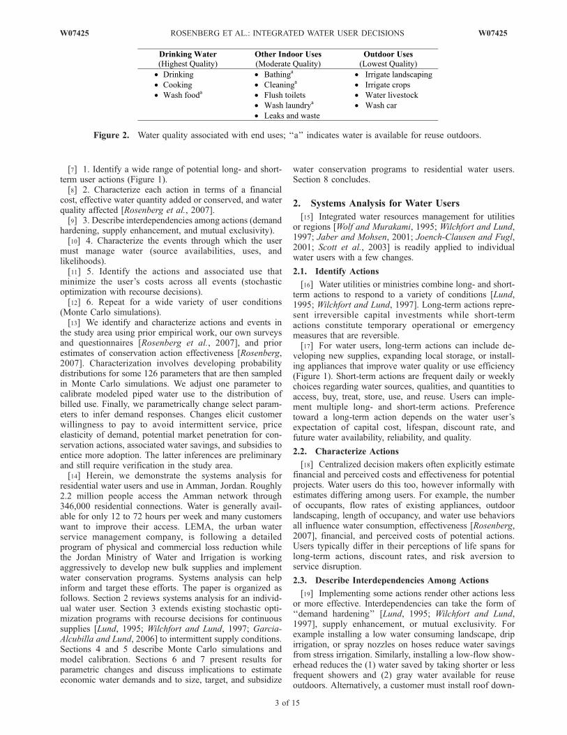
mittent supply system to consider numerous, interdependentwater user behaviors. We present a systems analysis thatintegrates multiple sources having different costs, availabil-ities, reliabilities, and qualities; many conservation options;and actions that improve local storage or water quality(Figure 1). We also embed uses that accommodate differentwater qualities (Figure 2). Integration helps quantifydemand responses for indoor and outdoor uses over differ-ent time horizons and how customers may respond toconservation incentives embedded in a tariff structure.[6] The systems analysis applies integrated approaches

typically made at regional or utility scales [Wolf andMurakami, 1995; Wilchfort and Lund, 1997; Jaber andMohsen, 2001; Joench-Clausen and Fugl, 2001; Scott et al.,2003] to individual users. It works as follows:

1Department of Civil and Environmental Engineering, University ofCalifornia, Davis, California, USA.

2Interdisciplinary Research Associates, Amman, Jordan.3Water Demand Management Unit, Ministry of Water and Irrigation,

Amman, Jordan.

Copyright 2007 by the American Geophysical Union.0043-1397/07/2006WR005340$09.00

W07425

WATER RESOURCES RESEARCH, VOL. 43, W07425, doi:10.1029/2006WR005340, 2007ClickHere

for

FullArticle

1 of 15

http://dx.doi.org/10.1029/2006WR005340

Figure

1.

Potential

managem

entactionsforwater

users

inAmman,Jordan.

2 of 15

W07425 ROSENBERG ET AL.: INTEGRATED WATER USER DECISIONS W07425

[7] 1. Identify a wide range of potential long- and short-term user actions (Figure 1).[8] 2. Characterize each action in terms of a financial

cost, effective water quantity added or conserved, and waterquality affected [Rosenberg et al., 2007].[9] 3. Describe interdependencies among actions (demand

hardening, supply enhancement, and mutual exclusivity).[10] 4. Characterize the events through which the user

must manage water (source availabilities, uses, andlikelihoods).[11] 5. Identify the actions and associated use that

minimize the user’s costs across all events (stochasticoptimization with recourse decisions).[12] 6. Repeat for a wide variety of user conditions

(Monte Carlo simulations).[13] We identify and characterize actions and events in

the study area using prior empirical work, our own surveysand questionnaires [Rosenberg et al., 2007], and priorestimates of conservation action effectiveness [Rosenberg,2007]. Characterization involves developing probabilitydistributions for some 126 parameters that are then sampledin Monte Carlo simulations. We adjust one parameter tocalibrate modeled piped water use to the distribution ofbilled use. Finally, we parametrically change select param-eters to infer demand responses. Changes elicit customerwillingness to pay to avoid intermittent service, priceelasticity of demand, potential market penetration for con-servation actions, associated water savings, and subsidies toentice more adoption. The latter inferences are preliminaryand still require verification in the study area.[14] Herein, we demonstrate the systems analysis for

residential water users and use in Amman, Jordan. Roughly2.2 million people access the Amman network through346,000 residential connections. Water is generally avail-able for only 12 to 72 hours per week and many customerswant to improve their access. LEMA, the urban waterservice management company, is following a detailedprogram of physical and commercial loss reduction whilethe Jordan Ministry of Water and Irrigation is workingaggressively to develop new bulk supplies and implementwater conservation programs. Systems analysis can helpinform and target these efforts. The paper is organized asfollows. Section 2 reviews systems analysis for an individ-ual water user. Section 3 extends existing stochastic opti-mization programs with recourse decisions for continuoussupplies [Lund, 1995; Wilchfort and Lund, 1997; Garcia-Alcubilla and Lund, 2006] to intermittent supply conditions.Sections 4 and 5 describe Monte Carlo simulations andmodel calibration. Sections 6 and 7 present results forparametric changes and discuss implications to estimateeconomic water demands and to size, target, and subsidize

water conservation programs to residential water users.Section 8 concludes.

2. Systems Analysis for Water Users

[15] Integrated water resources management for utilitiesor regions [Wolf and Murakami, 1995; Wilchfort and Lund,1997; Jaber and Mohsen, 2001; Joench-Clausen and Fugl,2001; Scott et al., 2003] is readily applied to individualwater users with a few changes.

2.1. Identify Actions

[16] Water utilities or ministries combine long- and short-term actions to respond to a variety of conditions [Lund,1995; Wilchfort and Lund, 1997]. Long-term actions repre-sent irreversible capital investments while short-termactions constitute temporary operational or emergencymeasures that are reversible.[17] For water users, long-term actions can include de-

veloping new supplies, expanding local storage, or install-ing appliances that improve water quality or use efficiency(Figure 1). Short-term actions are frequent daily or weeklychoices regarding water sources, qualities, and quantities toaccess, buy, treat, store, use, and reuse. Users can imple-ment multiple long- and short-term actions. Preferencetoward a long-term action depends on the water user’sexpectation of capital cost, lifespan, discount rate, andfuture water availability, reliability, and quality.

2.2. Characterize Actions

[18] Centralized decision makers often explicitly estimatefinancial and perceived costs and effectiveness for potentialprojects. Water users do this too, however informally withestimates differing among users. For example, the numberof occupants, flow rates of existing appliances, outdoorlandscaping, length of occupancy, and water use behaviorsall influence water consumption, effectiveness [Rosenberg,2007], financial, and perceived costs of potential actions.Users typically differ in their perceptions of life spans forlong-term actions, discount rates, and risk aversion toservice disruption.

2.3. Describe Interdependencies Among Actions

[19] Implementing some actions render other actions lessor more effective. Interdependencies can take the form of‘‘demand hardening’’ [Lund, 1995; Wilchfort and Lund,1997], supply enhancement, or mutual exclusivity. Forexample installing a low water consuming landscape, dripirrigation, or spray nozzles on hoses reduce water savingsfrom stress irrigation. Similarly, installing a low-flow show-erhead reduces the (1) water saved by taking shorter or lessfrequent showers and (2) gray water available for reuseoutdoors. Alternatively, a customer must install roof down-

Figure 2. Water quality associated with end uses; ‘‘a’’ indicates water is available for reuse outdoors.

W07425 ROSENBERG ET AL.: INTEGRATED WATER USER DECISIONS

3 of 15

W07425

spouts and storage before collecting and using rainwater. Auser can install a water-efficient semiautomatic or automaticlaundry machine, not both. Interdependencies criticallydepend on the actions under consideration. In the Amman,Jordan example, we consider 42 interdependencies.

2.4. Characterize Events for Which the System MustAdapt

[20] Water systems must adapt to events that decreasebulk supplies (during droughts or dry seasons) or increaseuse (peak load). Water system managers often characterizeevents by water availabilities (volumes) and likelihoods(probabilities). Managers seek to economically serve drinking-quality water to all users regardless of use.[21] Water users also face complex water-related events.

In Jordan, intermittent piped service, service disruptions,uncertain alternative supplies, and variable costs shapewater availability and likelihoods. Increased use (householdguests) and different uses accommodating different waterqualities (Figure 2) often force users to seek alternativesources when availability is limited. Event characteristicstypically differ among users.

2.5. Suggest Mixes of Actions

[22] Identifying the potential actions, costs, effectiveness,interdependencies, uses, events, and event probabilities asdiscussed above allows a water user to frame their choice ofwater management actions in terms of service availability,reliability, quality, and cost. We now describe in greaterdetail the optimization model to represent choices.

3. Stochastic Optimization With RecourseDecisions

[23] We formulate the water user’s decision problem as atwo-stage stochastic program. The program identifies andquantifies the mix of actions that minimize a water user’sexpected costs to meet all water quality uses across differentwater availability events. Events are described by watersource availability (volume) and likelihood (probability).[24] Decision staging works by partitioning actions into

two types. Long-term (first- or primary-stage) actions applyfor all events. Then, additional short-term (secondary- orrecourse-stage) actions are implemented in particular eventsto cover remaining uses not met by long-term actions.Together, long-term actions plus sets of short-term actionsfor each event constitute the mix of actions that respond tothe probability distribution of water availability. As wateravailability or reliability decreases, water users adopt in-creasingly expensive short-term actions.[25] The program extends a prior two-stage linear pro-

gram of water user with continuous supplies [Garcia-Alcubilla and Lund, 2006] to include an expanded set ofsources, storage, and water quality improvement actions(Figure 1); a variety of drinking, indoor, and outdoor wateruses that accommodate different water qualities (Figure 2);interdependencies among actions; limited source availabil-ity and reliability; and nonlinear costs.[26] These extensions reflect actions, uses, conditions,

and costs (Appendix A) typical for residential water userswith intermittent supplies in Jordan. The model is readilyadapted for other users (commercial, industrial, agricultural,etc.) and other locations.

3.1. Decision Variables

[27] The decision variables are L = vector of implemen-tation levels for long-term actions (binary or integer), S =matrix of water volumes for short-term actions in each event(m3 event�1), and X = matrix of supply volumes allocatedto each water quality use in each event (m3 event�1).[28] In the notation below, lt, st, e, and u are, respectively,

indices for long- and short-term actions, events, and waterquality uses. Llt, Sst,e, and Xu,e are individual decisionelements of L, S, and X.

3.2. Model Formulation

[29] Risk-neutral water users minimize their annualexpected long- and short-term water management costs, Z($ yr�1). With c1 (L) = annualized costs to implement long-term actions ($ year�1), c2,e (S) = event-specific costs toimplement short-term actions ($ event�1), pe = probabilityof event e (unitless, but

Pe

pe = 1 and 0� pe� 1, 8e), and a =constant that relates the periods of short- and long-termactions (events yr�1), the objective can be expressed as

Minimize Z ¼ c1 Lð Þ þ a �X

e

pe � c2;e Sð Þ: ð1Þ

[30] Event probabilities (pe) weight event-specific costs(c2,e) associated with short-term actions [Lund, 1995;Wilchfort and Lund, 1997]. Piped water charges are acomponent of c2,e. Long-term costs (c1) include networkconnection fees and other capital expenses.[31] The objective function (equation (1)) is subject to

several constraints.[32] 1. Water supplies, su,e (S, X) (m3 event�1), must

satisfy the initial estimate of water use, du,e (m3 event�1) for

each quality use u in each event e, reduced by water savedfrom conservation actions, hu,e (L, S) (m

3 event�1),

su;e S;Xð Þ du;e � hu;e L; Sð Þ; 8e8u: ð2Þ

[33] This specification disaggregates initial estimates intoseparate estimates for eachwater quality use u in each event e.Users meet estimates by acquiring and/or conserving water.The physical volume allocated, su,e, is the optimal water use.However, this use can (and often is) less than the initialestimate (du,e).[34] 2. Each long-term action Llt has a fixed upper limit of

implementation, ult (integer),

Llt � ult; 8lt: ð3Þ

[35] 3. Each short-term action Sst has an availability orfixed upper limit of implementation, ust,e (m

3 event�1), thatcan potentially decrease or increase, gst,e (L, S, X) (m3

event�1), on the basis of interdependencies with otheractions,

Sst;e � ust;e þ gst;e L; S;Xð Þ; 8e 8st: ð4Þ

[36] Intermittently available sources have different upperlimits (ust,e) in different events e. The interdependency func-tion, gst,e, is an n 1 vector, n = rank (L) + rank (S) + rank (X),whose elements describe pair-wise interdependencies with

4 of 15


the short-term action Sst,e. Negative elements represent de-mand hardening relations (reduce the upper limit), positiveelements supply enhancement relations, and zero values (thevast majority) reflect no relation. For mutually exclusiverelations, gst,e is equal but opposite to ust,e.[37] 4. In each event e, the user must direct all primary

(rain and municipal water) and secondary (from vendors orneighbors) supplies (together, PSSs) to one or more waterquality uses u, allowing high-quality water to meet lower-quality uses,

X

u

Xu;e �X

st2PSSsSst;e; 8e: ð5Þ

[38] 5. Local storage capacity, vstor (L) (m3 event�1),associated with long-term actions limits the total volume ofprimary supplies (PSs) in each event e. After exhaustingprimary supplies, the user must draw on secondary sources,

X

st2PSsXst;e � vstor Lð Þ; 8e: ð6Þ

[39] 6. Finally, all decision variables must be positive:

Llt 0; 8lt; Sst;e 0; 8st8e; Xu;e 0; 8u8e: ð7Þ

3.3. Model Discussion

[40] In the Amman, Jordan example, equations (1)–(7)are setup as a mixed integer nonlinear program in theGeneric Algebraic Modeling System (GAMS) [Brooke etal., 1998] and solved with DICOPT [Grossmann et al.,2002]. However, when the cost (c1 and c2,e), supply (su,e),conservation (hu,e), and interdependency (gst,e) functions arelinear and separable by management action, the program ismore easily solved as a mixed integer linear program.

4. Monte Carlo Simulations

[41] Action costs (c1 and c2), initial estimates of water use(du,e), conservation (hu), water availabilities/upper limits onactions (ust,e and ult), event probabilities (pe), and actioninterdependencies (gst,e) vary among customers. We embedthe optimization in Monte Carlo simulations (MCS) ofcustomers to represent customer heterogeneity, but maintainconsistency in each input set. MCS takes three steps.[42] First, we develop an empirical basis of water user

behaviors and conditions from 9 prior studies in Amman,Jordan [Theodory, 2000; Iskandarani, 2002; Snobar, 2003;Interdisciplinary Research Consultants, 2004; Rosenberg etal., 2007] (see also Jordan Meteorological Department(JMD), Rainfall, 2000, http://met.jometeo.gov.jo/; Centerfor Study of the Built Environment, Water conservinglandscapes, 2004, http://www.csbe.org/water_conserving_landscapes/index.html; and Department of Statistics(DOS), Amman, Jordan, Urban agriculture survey, 1999,http://www.dos.gov.jo/sdb/env/env_e/home.htm and Thepreliminary results of the population and housing census,2004, http://www.dos.gov.jo; and Academy for EducationalDevelopment, 2001, Capacity building project in Amman,Irbid, and Aqaba, report, 12 pp., Water Efficiency and

Public Information for Action, U.S. Agency for InternationalDevelopment, Amman, Jordan, http://pdf.dec.org/pdf_docs/PNADB469.pdf). Absent other data, we make engineeringestimates [Rosenberg, 2007]. Second, we use the empiricaldata to develop probability distributions for some 126parameters that influence a customer’s water use, wateravailability or reliability, effectiveness of one or moreconservation actions, or action costs (Appendix A). A prob-ability distribution characterizes each parameter with arange and likelihood of values the parameter can take.Third, we sample from each distribution, combine sampledvalues in explicit ways to estimate optimization modelinputs, then optimize for the customer-specific inputs. Werepeat step 3 for a large number of simulated customers thenobserve averages and distributions of the optimized results.[43] Empirical parameter distributions were sampled and

combined in Excel and then fed to GAMS. Below, wedescribe calculations for optimization model inputs and howMCS allows detailed specification of end uses and corre-lated and conditional sampling. In these calculations, wedefine the event period as a week based on the weeklyrationing schedule for piped water.[44] We calculate action costs (c1 and c2,e) by sampling

from normal or uniform distributions of capital costs, lifespans, and operational costs [Rosenberg et al., 2007](Appendix A). The price schedule for piped water use andsome operational costs are fixed and constant among cus-tomers. We use the 2001–2005 price schedule. During thisperiod, four increasing blocks had, respectively, fixed, var-iable, and quadratic charges for water use below 20, 40, and130m3 per customer per quarter. Use above 130m3 reverted toa variable charge (for formulas, see Rosenberg et al. [2007]).[45] We make initial estimates of water use as products

and summations of the relevant sampled empirical param-eter values. For example, the initial estimate of bathroomfaucet water use, dBathFaucet (m

3 customer�1 week�1), is

dBathFaucet ¼7

1000PNð Þ PYð Þ PGð Þ; ð8Þ

where PN = the flow rate of the existing bathroom faucet(l min�1), PY = wash time (min person�1 d�1), and PG =household size (persons). (The capital letters PN, PY, etc.reflect notation common to the probability literature where acapital letter; that is, PN, means the parameter is uncertain.Before sampling, use is also uncertain. Appendix Adescribes the parameters. Hereafter, PN, refers to parameterN in Appendix A; similarly for other subscripts). Combin-ing initial estimates for bath faucet, toilet, shower, kitchenfaucet, floor washing and laundry uses gives the total indoorwater use, dindoor,e (m3 customer�1 week�1). Except forshowering and outdoor irrigation (see below), we assumeinitial estimates are the same across all events.[46] We use previously reported effectiveness functions

for seven long-term conservation actions [Rosenberg,2007]. For example, the water saved when retrofitting abathroom faucet with a faucet aerator, WFaucetRetroBath (m3

customer�1 yr�1) is

WFaucet RetroBath ¼365

1000PN � PANð Þ PYð Þ PGð Þ; ð9Þ


5 of 15

W07425

where PAN = faucet aerator flow rate (l min�1), and PN,, PY,and PG as defined previously.[47] Similar parameter combinations shape initial esti-

mates of other end uses and the effectiveness of relatedconservation actions with several modifications. (1) Wedisaggregate shower use and effectiveness of related con-servation actions by summer and winter differences inshower behavior (PU and PV). (2) Toilet water use andeffectiveness of toilet conservation actions key to toiletflush volume (PO). Customers with squat (Arabic) toilets(first category of PO) have zero effectiveness for toiletconservation actions. (3) Laundry water use multiplies bya rinse factor (PAL) when the household has a semiautomaticmachine (category 2 of PAJ). (4) The drinking water useestimate was a linear combination of household size (PG)and a random effect (PH). This relation was determined byregressing reported household drinking water consumptionand purchases [Rosenberg et al., 2007] against householdsize. Household size explained 59% of variability. (5) Irriga-tion water use ceases during winter. (6) Piped water andtanker truck water availabilities were unconstrained. How-ever, in the summer event with limited availability, house-holds can only use 2 m3 per week of piped water. Borrowingwater was available only to the portion of households thatfind the practice acceptable (PAH); borrowing extends avail-ability up to 0.3 m3 per event. (7) An occupancy parameter(PI) serves as a global multiplier on the effectiveness of allconservation actions and all water uses except outdoorirrigation. The multiplier was zero, 0.5, and 1.0 when PI

was sampled, respectively, as vacant, partial, or full occu-pancy. Partial occupancy indicates that only some householdmembers live at the house full time, or, that the householdoccupies the house part time and other times the house isempty with little/no water use.[48] In the Amman example, we consider three events:

weeks of summer use with (1) limited and (2) unlimitedpiped water availability, and (3) winter use with wintersupplies. We calculate probabilities for these events fromthe sampled number of irrigation weeks in summer withlimited availability (PC), the sampled remaining irrigation

season (PB � PC), and noting that all event probabilitiesmust sum to one:

pSummer Limited Availability ¼PCð Þa

ð10aÞ

pSummer Unlimited Availability ¼PBð Þ � PCð Þ

að10bÞ

pWinter ¼ 1� pSummer Unlimited Availability � pSummer Limited Availability:

ð10cÞ

[49] Equations (8)–(10) and the paragraph of modificationsshow that MCS allows detailed and correlated customer-specific specification of optimization model inputs includingwater use. For example, several effectiveness and use func-tions are conditioned on existing water use appliances (toiletsand laundry). Other parameters appear repeatedly in the wateruse and effectiveness functions and indicate these optimiza-tion input parameters are strongly correlated (PN, PY, and PG

in (8) and (9) for faucet use and related conservation actions).Regression or customer preference models do not typicallyinclude these details or interdependencies.

5. Model Calibration

[50] We calibrate the cumulative distribution of modeledpiped water use to use billed by Amman residential cus-tomers in 2005 (Figure 3). Calibration included 500 MonteCarlo simulated customers and set upper limits for all long-term conservation actions to zero (ult = 0 in equation (3)).This setting represents current conditions with limitedadoption of long-term conservation actions (limited adop-tion is still represented by low sample values for techno-logical parameters). Calibration varied only the fractions ofvacant and partially occupied households (PG) by trial anderror to maximize the Kolmogorov-Smirnov goodness of fit

Figure 3. Model calibration against cumulative distribution of billed residential water use in 2005 forresidential customers in Amman, Jordan.

6 of 15


(K-S Test) between the billed and modeled water usedistributions.[51] Occupancy was chosen as the calibration parameter

since the number of residential connections (customers)differs from the census of total and vacant housing units(O. Maghrabi, personal communication, 2006; and Depart-ment of Statistics, Amman, Jordan, The preliminary resultsof the population and housing census, 2004, http://www.dos.gov.jo). The difference is likely due to differentsampling frames (i.e., some connections serve multiplehousing units). Calibration found the percentages of vacantand partially occupied connections as 10% and 15%,respectively.[52] The K-S Test (D statistic = 0.019; n1 = 20; n2 = 500)

indicates that the distributions of billed and modeled pipedwater use are similar at the 98% significance level(Figure 3). Both distributions skew heavily toward largefractions of customers that use less than 40 m3 per customerper quarter and smaller fractions who use considerablygreater volumes. Billed and modeled uses average, respec-tively, 39.6 and 37.8 m3 per customer per quarter, adifference of 4%.

6. Results for Parametric Changes

[53] The calibration model run described above repre-sents a base case with existing (limited) adoption of long-term conservation actions. Parametrically changing basecase parameter value(s) can show how availability, pricing,and conservation campaigns may influence water use. Thesechanges are used to infer economic effects such as willing-ness to pay (WTP) to avoid limited piped water availability,price elasticity of demand, and potential market penetrationrates for conservation actions.

6.1. Municipal Water Availability

[54] We increased piped water availability from 2 to 20 m3

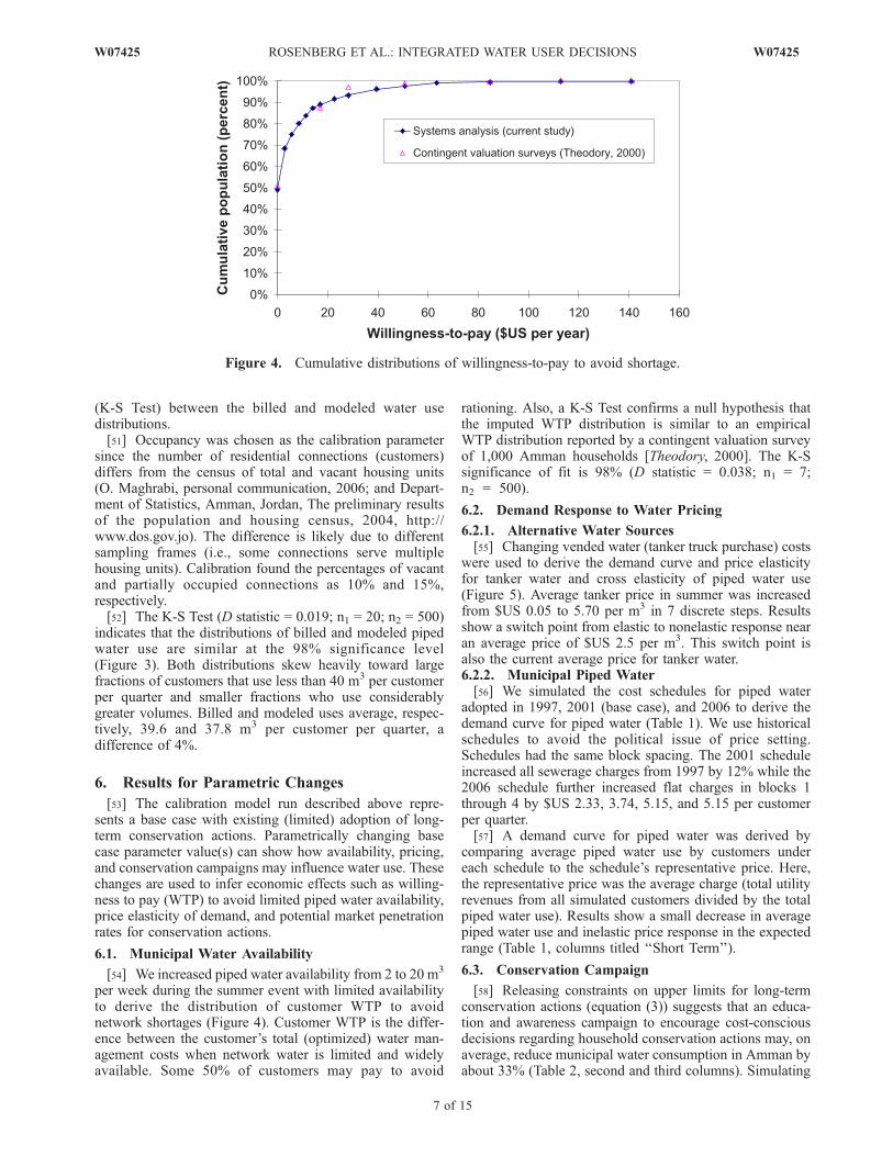
per week during the summer event with limited availabilityto derive the distribution of customer WTP to avoidnetwork shortages (Figure 4). Customer WTP is the differ-ence between the customer’s total (optimized) water man-agement costs when network water is limited and widelyavailable. Some 50% of customers may pay to avoid

rationing. Also, a K-S Test confirms a null hypothesis thatthe imputed WTP distribution is similar to an empiricalWTP distribution reported by a contingent valuation surveyof 1,000 Amman households [Theodory, 2000]. The K-Ssignificance of fit is 98% (D statistic = 0.038; n1 = 7;n2 = 500).

6.2. Demand Response to Water Pricing

6.2.1. Alternative Water Sources[55] Changing vended water (tanker truck purchase) costs

were used to derive the demand curve and price elasticityfor tanker water and cross elasticity of piped water use(Figure 5). Average tanker price in summer was increasedfrom $US 0.05 to 5.70 per m3 in 7 discrete steps. Resultsshow a switch point from elastic to nonelastic response nearan average price of $US 2.5 per m3. This switch point isalso the current average price for tanker water.6.2.2. Municipal Piped Water[56] We simulated the cost schedules for piped water

adopted in 1997, 2001 (base case), and 2006 to derive thedemand curve for piped water (Table 1). We use historicalschedules to avoid the political issue of price setting.Schedules had the same block spacing. The 2001 scheduleincreased all sewerage charges from 1997 by 12% while the2006 schedule further increased flat charges in blocks 1through 4 by $US 2.33, 3.74, 5.15, and 5.15 per customerper quarter.[57] A demand curve for piped water was derived by

comparing average piped water use by customers undereach schedule to the schedule’s representative price. Here,the representative price was the average charge (total utilityrevenues from all simulated customers divided by the totalpiped water use). Results show a small decrease in averagepiped water use and inelastic price response in the expectedrange (Table 1, columns titled ‘‘Short Term’’).

6.3. Conservation Campaign

[58] Releasing constraints on upper limits for long-termconservation actions (equation (3)) suggests that an educa-tion and awareness campaign to encourage cost-consciousdecisions regarding household conservation actions may, onaverage, reduce municipal water consumption in Amman byabout 33% (Table 2, second and third columns). Simulating

Figure 4. Cumulative distributions of willingness-to-pay to avoid shortage.


7 of 15

W07425

the three historic rate structures for this case shows aslightly more elastic price response and a significant shiftinward (left) of the demand curve (Table 1, columns titled‘‘Long Term’’). This analysis provides a way to differentiateshort- and long-term demand curves (i.e., before and afteradopting long-term conservation actions). A conservationcampaign would incidentally reduce tanker truck water useby more than 60%, decrease customer’s overall water-related expenditures by 35%, and, alas, reduce utilityrevenues nearly 60% (due to the convex rate structure)![59] Interestingly, a small fraction of customers with very

significant water savings drive reductions in piped water use(Figure 6). For example, just 38% of the Monte Carlosimulated customers retrofit showerheads. The adoptingcustomers average water savings of 50 m3 per customerper year with savings ranging from 5 to more than 100 m3

per customer per year. Other actions such as installing dripirrigation or xeriscaping have low market penetration rates,but are extremely effective for customers who adopt. Thesedistributions suggest that a targeted conservation campaigncan achieve significant water savings with concentratedeffort.[60] Examining the reduced costs for long-term conser-

vation actions identifies drip irrigation, kitchen faucet

aerators, and toilet dual flush mechanisms as actions thewater utility might target with financial incentives (Figure 7).The reduced cost is the decrease in cost required for thecustomer to benefit overall to adopt the action. It is alsothe customer’s willingness to accept, or, alternatively, thesubsidy to entice adoption. The utility may find it cheaper topay customers to adopt these conservation actions to reduceuse rather than produce, treat, and deliver the equivalentwater volume.

7. Discussion

[61] A systems analysis estimates water use with inter-mittent supplies by considering interdependent effects ofnumerous water user behaviors. Behaviors include infra-structure investments and short-term coping strategies suchas accessing multiple sources having different availabilities,reliabilities, and qualities, conservation options, local stor-age, and water quality improvements. The analysis embedsend uses requiring various water qualities and variablecosts, including block rate structures. Model calibrationreproduces both the mean and distribution of existing pipedwater use in Amman, Jordan. It simultaneously estimatesuse for a wide range of alternative supplies (vended water,rainwater, gray water, etc.). Further parametric changespermit study of economic water demands, including will-ingness to pay for increased availability, price elasticity ofdemand, and cost, water savings, and potential penetrationrates for conservation actions. We discuss each of these

Figure 5. Elasticity and cross elasticity of tanker truck water price.

Table 1. Demand Response Simulating Piped Water Use for

Different Historical Rate Structuresa,b

Demand CurveComponent

Short Term, BeforeConservation

Long Term, WithConservation

1997 2001 2006 1997 2001 2006

Piped water use peraverage householdper year, m3

152.9 152.4 151.7 101.7 100.8 99.3

Representative price,$US per m3

0.80 0.86 0.95 0.80 0.86 0.95

Point elasticity at 2001price and use

�0.05 �0.14

aRepresentative price equals total utility revenues divided by total billedwater use.

bLong- and short-term curves plot at same representative prices.

Table 2. Average Responses to Conservation Efforts

Indicator

Short Term,Before

Conservation

Long Term,After

Conservation

Piped water use m3 customer�1 yr�1 152.0 100.7Tanker truck use m3 customer�1 yr�1 9.2 1.5Rainwater collected, m3 customer�1 yr�1 0.0 4.7Gray water reused, m3 customer�1 yr�1 0.0 3.9Expenditures, $US customer�1 yr�1 232.1 149.3Utility revenues, $US customer�1 yr�1 101.8 41.2

8 of 15


results plus limitations. We emphasize that the price andconservation results still require empirical verification.

7.1. Increased Availability and Willingness to Pay

[62] Increasing piped water availability is used to derive adistribution of customer willingness to pay (WTP) to avoidrationing. This distribution reproduces WTP reported by aprior contingent valuation study (Figure 4). An advantage ofsystems analysis is ability to post facto specify and respecifyWTP intervals with greater resolution. The analyst simplyincreases the number of Monte Carlo simulations and/ordecreases the spacing used to tally MCS results. This easecontrasts with difficulties for surveyors posing contingentvaluation questions to respondents. They must pose new,narrower questions again to respondents. Also, cost param-eters (Appendix A) excluded hassle, so customers may havegreater WTP than suggested by the model or the prior survey.

7.2. Price Elasticity of Demand

[63] Piped water use was estimated for several historicrates structures. Comparing use and the ‘‘representativeprice’’ for the rate structure permits estimating a priceelasticity of demand. However, there are numerous waysto post facto calculate the ‘‘representative price.’’ Forexample, averaging the average prices paid by each cus-tomer gives a slightly more elastic price response. Substi-tuting marginal prices gives an infinitely elastic response (inthe Amman example, fixed charges increase but the variable(marginal) charges do not). For conservation efforts, usinglower prices associated with lower use achieved by conser-vation gives a more elastic price response. These differentinterpretations of price response are artifacts of (1) customerbehavior (ability to substitute other sources and conserva-tion actions), (2) the fixed and variable charges in the

Figure 6. Estimated market penetration and water savings for conservation actions in Amman, Jordan.Circles show average, and error bars show 10th and 90th percentiles of Monte Carlo simulations.

Figure 7. Average subsidies required to entice additional customers to install water-efficient appliances.For actions below LEMA production cost curve, percent indicates fraction of households that arepotentially enticed.


9 of 15

W07425

existing schedule, and (3) method to calculate a ‘‘represen-tative’’ price for the schedule.[64] Block spacing can also create an artifact (although

not in the Amman example). A wider block captures morecustomers and pulls the representative price closer to pricesfaced by customers in that block. This artifact also manifestswith customers who switch blocks.[65] These issues identify an important limitation of

demand curves under block pricing. Reducing multipledegrees of freedom (block spaces, fixed, and variablecharges) to a single representative price influences theinterpretation of price response.

7.3. Conservation Campaigns

[66] Allowing users to adopt long-term conservationactions (when they find it cost effective) predicts significantwater savings despite low adoption rates. At most, 38% ofcustomers retrofit showerheads, 33% install aerators onkitchen faucets, 18% catch rainwater, 4% retrofit semiauto-matic laundry machines, 0.5% xeriscape, etc. These find-ings suggest water conservation campaigns should targetcustomers who will realize large financial and water sav-ings. Obviously, success requires identifying real customerswith significant potential to save water and money, deter-mining what action(s) they should adopt, motivating adop-tion, and verifying that estimated savings translate to actualsavings. Rosenberg [2007] suggests using surrogate dataindicators, customer surveys, and water audits to identifyhigh potential customers and actions.[67] Numerically integrating the distributions of water

savings shown in Figure 6 gives conservation programsizing curves (Figure 8). The curves suggest the minimalmarket penetration needed to meet a conservation objective[Rosenberg, 2007]. Minimal market penetration is achievedby ordering customers (x axis in Figure 8) left to right fromthe largest down to the smallest (zero) water savings. At

first, sizing curves are steep, but then flatten to the averageeffectiveness achieved with full participation (this averageexactly equals the product of (1) average water savings forimplementing customers and (2) the market penetration rateshown in Figure 6). Here, average effectiveness estimatesby systems analysis are much lower than estimates forindividual actions that ignore implementation costs andinterdependencies [Rosenberg, 2007]. For example, Rosenberg[2007] reports average savings of 45 m3 per customer peryear to retrofit showerheads or kitchen faucets compared tocurrent estimates of 19.4 and 11.6 m3 per customer per year,respectively. The decrease occurs because systems analysisscreens out customers with high effectiveness but insuffi-cient financial incentive to adopt. Also, customers whoadopt cost-effective conservation action(s) and then haveno incentive to further conserve. Despite decreases, systemsanalysis still reproduces the more general finding: targetconservation actions to customers who will save the mostwater and money.[68] Examining the reduced costs associated with conser-

vation actions also shows the Amman water provider mightfind it cheaper to subsidize some customer conservation ratherthan provide the equivalent water volume. The utility couldoffer subsidies as a rebate or credit on the water bill tocustomers who verify installation. In Amman, verificationwill be critical and is potentially compromised by wasta(favors). Tomake subsidiesmore effective, governance shouldimprove employee accountability, reward performance, en-force water conserving plumbing codes, restrict the import andmanufacture of inefficient water appliances, label efficientappliances, and raise awareness about the financial savingsassociated with purchasing efficient appliances.

7.4. Further Methodological Limitations

[69] First, the optimization assumes expected, financialcost-minimizing customer decisions with full information

Figure 8. Sizing curves for water conservation programs. X axis is ordered by customers from highestto lowest conservation action effectiveness.

10 of 15


even though customers may include time, hassle, and socialdesirability values in their decisions. However, a cost-minimizing model is not necessarily misspecified. Rather,cost-minimizing behavior is borne out empirically throughmodel calibration so customers in Amman behave as if theyminimize their costs. Hewitt and Hanemann [1995] deploythis as if argument to justify their Discrete/Continuouschoice water use model. For the uncalibrated conservationcampaign results, including convenience costs, hassle, andother factors may well reduce modeled adoption rates andwater savings. Still, this reduction does not compromise themore general recommendation reached after examining theMonte Carlo distribution of responses: target conservationactions to customers who will save the most water andmoney.[70] Second, initial estimates of water use set upper

bounds for the optimal use (equations (2) and (8)). Cus-tomers can only choose from an exhaustive set of sourcesand conservation actions to set their use at or below theinitial estimate. Yet customers may also benefit to expandtheir garden area or take longer or more frequent showers,etc. The upper bound means that availability runs should bestrictly interpreted as willingness to pay to avoid rationing.Quite possibly, use could significantly increase shouldpiped water become widely available.[71] Third, the two limitations above suggest further work

to develop a utility-maximizing rather than cost-minimizingdecision criterion. This change requires estimating theutility contributions of hassle, social desirability for eachaction, plus specifying variability among customers. Yetlittle empirical data exists to describe these contributions.Estimating contributions requires assembling a large dataset, specifying a regression model, and teasing apart diverseand potentially interdependent responses. These tasks re-quire significant effort beyond the scope of the currentstudy.[72] Fourth, significant unaccounted-for and nonrevenue

water loss in Amman means actual and billed use differ[Griffen, 2004]. Fortunately, systems analysis already includeslosses from physical leakage, billing, and metering errors.Physical leakage reduces piped water availability and isrepresented by limited availability events in optimizations.Customers react to these conditions. Calibration capturesmetering and billing errors by attributing these losses to partialor vacant occupancy. Also, absent empirical data on illegalconnections, we exclude thieving customers. With data onillegal connections, we could better specify the parameterdistribution to borrow water (PAH, a free source).[73] Finally, targeted conservation programs substantially

reduce piped water use and erode utility revenue. InAmman, a convex (quadratic) price schedule means high-use customers disproportionately contribute to utility rev-enues and have the most potential to save water and money.To reduce use and protect revenue, a utility may encouragecustomers with low use to conserve further. Such targetingraises social and equity issues. It illustrates that pricing,source availabilities, conservation options, and utility rev-enues interrelate and must be considered jointly to developcoherent water conservation programs. Minimally, utilityrevenue requirements suggest needs for further analysis at awider scale. One should compare costs and water savings of

targeted conservation programs with alternatives that in-crease bulk supplies or reduce physical losses.

8. Conclusions

[74] This paper extends water use modeling in an inter-mittent supply system to consider numerous, interdependentwater user behaviors. Behaviors include water conservation,improving local storage and water quality, and accessingmultiple sources having variable availabilities, reliabilities,qualities, and costs. An optimization program suggests themix of actions a user should adopt to reduce expected watermanagement costs given a probability distribution of pipedwater availability and action interdependencies such asdemand hardening, supply enhancement, and mutual exclu-sivity. Monte Carlo simulations show average citywideeffects and distributions of customer responses, includingpiped water use. Parametrically changing model parametersallows inferring potential economic effects for several wateravailability, pricing, and conservation efforts. The primaryresults, findings, limitations, and recommendations forfuture work are as follows.[75] 1. The modeling approach reproduces both the

existing average and distribution of piped water use forresidential customers in Amman, Jordan.[76] 2. Willingness to pay to avoid rationing closely

matches reports from a contingent valuation method. How-ever, significant untapped or unmet uses may exist forcontinuous supplies.[77] 3. Price response is highly inelastic. However, the

rate structure (block spaces, fixed and variable charges)complicates interpretation of price response.[78] 4. In Amman, a conservation campaign may signif-

icantly reduce piped water use.[79] 5. Campaigns should target select customers that

show the most potential to save water and money.[80] 6. In limited cases, the utility can subsidize custom-

ers to install water efficient appliances to realize furtherwater savings. Successful implementation will require im-proving employee accountability.[81] 7. Targeted conservation programs will reduce utility

revenues. Balancing these impacts with the benefits ofreducing water use requires further analysis at a widerutility scale.[82] 8. Results for pricing and conservation efforts still

require empirical verification. Including hassle, time, andother factors may reduce adoption rates.[83] Overall, systems analysis helps model and understand

several complexities and impacts of water user behaviors.

Appendix A: Parameter Descriptions

[84] This appendix describes the parameters influencinginitial estimates of water use and conservation actioneffectiveness (Table A1) and action costs (Table A2).

Notation

a number of events per year.c1 annual cost of long-term actions, $ yr�1.

c2,e cost of short term actions in event e, $ event�1.du,e initial estimate of water quality use u in event

e, m3 event�1.


11 of 15

W07425

Table A1. Parameters Influencing Initial Estimates of Water Use and Conservation Action Effectiveness

Parameter UnitsLowValue

HighValue Average

StandardDeviation Distributiona Referenceb

GeographicA. Annual rainfall mm/yr 110.0 550.0 269.7 93.5 FG JMD (78 years)B. Irrigation season weeks/yr 20.0 35.0 - - UN engineering estimateC. Network shortages weeks/yr 0.5 - 3.0 - ED AED (344 households)D. Rainfall events number/yr 1.0 6.0 - - UN engineering estimate

DemographicE. Roof area of building m2 100.0 - 206.1 - ED DS99 (1,800 households)F. Households sharingbuilding

number/building 1.0 - 2.7 - ED DS04 (383,000 households)

G. Household size persons 3.0 - 5.1 - ED DS04 (383,000 households)H. Drinking waterrandom effects

l/event (43.4) 19.9 (0.0) 67.1 NM R07 (c. 28 persons)

I. Occupancy fraction - 1.0 - - HS (3) calibrated

TechnologicalJ. Garden area m2 - 300.0 111.3 103.2 FG DS99 (1,800 households)K. Number cars number of cars - - 1.3 0.5 FG AED (344 households)L. House water pressure bar 0.3 - 0.6 - ED Engineering estimate; func. of (F.)M. Shower flow rate- current device

l/min 6.0 20.0 - - UN IRC (c. 10 devices)

N. Faucet flow rate- current device


O. Toilet tank volume- current device

l/flush 5.5 15.0 - - HS (6) AED (344 households)

P. Laundry water use- current device

l/kg - - - - NM ARD (c. 20 devices); func. of (AJ.)

Q. Hose diameter inches 0.5 1.5 - - UN engineering estimateR. Bucket size gal 3.0 7.0 - - UN engineering estimateS. Water use - cons.auto laundry

l/kg 6.2 - 8.3 1.4 NM IRD (c. 20 devices)

BehavioralT. Length of shower(current)

min 1.5 - 8.5 - ED IRC (c. 10 devices)

T. Length of shower– currernt

min 1.5 - 8.5 - ED IRC (c. 10 devices)

U. Shower frequency– summer

number/week 1.0 - 3.6 - ED R07 (c. 28 persons)

V. Shower frequency– winter

number/week 1.0 - 0.4 - NM R07 (c. 28 persons)

W. Toilet flushes number/person/d 2.0 - 4.0 - ED S03 (30 households)X. Flushes requiringfull flush

fraction of flushes 0.3 0.7 - - UN engineering estimate

Y. Faucet use min/d/person 0.1 - 0.6 - ED S03 (30 households)Z. Car wash time min/use 5.0 15.0 - - UN AED (344 households)AA. Car washes washes/week - - 1.6 1.0 FG AED (344 households)AB. Irrigation frequency number/week 0.2 - 1.7 - ED AED (344 households)AC. Floor wash frequency number/week 1.0 7.0 - - UN engineering estimateAD. Irrigation applications hrs/week 0.2 - 1.7 - ED R07 (c. 28 pers.)AE. Bucket applicationto car

number buckets/car 2.0 5.0 - - UN engineering estimate

AF. Bucket applicationto floor

buckets/wash 1.0 - 5.0 - ED engineering estimate

AG. Kitchen faucet use min/d 1.0 - 14.4 - ED S03 (30 households)AH. Borrow m3/event 0.1 0.3 - - UN I02 (200 households)AI. Car wash method (1 = auto, 2 = bucket,

3 = hose)1.0 3.0 1.9 - HS (3) AED (344 households)

AJ. Laundry wash method (1 = hand, 2 = semi,3 = auto)

1.0 3.0 2.3 - HS (3) AED (344 households)

AK. Laundry weight kg/person/week 0.6 - 3.9 - UN R07 (c. 28 pers.)

Technological ModificationsAM. Shower flow rate- retrofit device


AN. Faucet flow rate- retrofit device


AO. Toilet flush rate- retrofit, full

l/flush 5.5 6.5 - - UN IRC (c. 20 devices)

AP. Toilet flush rate- retrofit, half

l/flush 2.0 3.0 - - UN engineering estimate

12 of 15


Table A1. (continued)


HighValue Average


AQ. House water pressure– reduced

bar 0.5 1.0 - - UN engineering estimate

AR. Irrigation rate - drip l/hr/mister 125.0 1,080.0 - - UN engineering estimateAS. Drip mister density number misters/50 m2 3.0 10.0 - - UN engineering estimateAT. Water use - conssemi-auto laundry

l/kg 3.3 - 5.1 1.5 NM IRC (c. 20 devices)

AU. Drinking watertreatment efficiency

fraction 0.3 0.8 - - UN R07 (c. 28 pers.)

AV. Toilet bottle size l/bottle 0.5 1.5 - - UN engineering estimateAW. Toilet bottlesinstalled

number 1.0 2.0 - - UN engineering estimate

Behavior ModificationAX. Faucet flow rate- partially open

l/min 2.0 8.0 - - UN engineering estimate

AY. Shower length– shortened

min 1.0 6.0 - - UN engineering estimate

AZ. Shower frequency– reduced

number/week 0.5 - 0.8 - ED engineering estimate

BA. Faucet wash timesaved

min/person/d 0.1 - 0.5 - ED engineering estimate

BB. Laundry frequency– reduced

fraction (curr. laundry) 0.1 0.5 - - UN engineering estimate

BC. Reduced irrigationtime - nozzle

min/use 0.5 - 3.0 - ED engineering estimate

BD. Reduced irrigationtime - stress irr.

min/use 1.0 - 10.0 - ED engineering estimate

aED = exponential decay, FG = fitted gamma, HS(x) = histogram with x categories, NM = normal, UN = uniform, and FV = fixed value (constant).bSample size is given in parentheses. JMD, Jordan Meteorological Department (2000); AED, Academy for Educational Development (2001); DS99,

Department of Statistics (1999); DS04, Department of Statistics (2004); R07, Rosenberg et al. [2007]; IRC, Interdisciplinary Research Consultants (2004);S03, Snobar [2003]; I02, Iskandarani [2002].

Table A2. Parameters Influencing Action Costs


HighValue Average


Capital Costs for Long-Term ActionsBE. Network connection $US - - 324.3 - FV R07BF. Roof tanks - 2 m3 size $US 91.7 - 104.3 14.3 NM R07 (c. 4 stores)BG. Roof tanks - 1 m3 size $US 53.6 - 64.2 8.9 NM R07 (c. 4 stores)BH. Ground tanks - 2 m3 size $US 97.3 - 110.0 14.3 NM R07 (c. 4 stores)BI. Cistern $US 620.4 - 972.9 641.5 NM R07 (c. 28 persons)BJ. Rainwater collection system $US 141.0 - 282.0 141.0 NM R07 (c. 4 stores)BK. Grey-water system $US - - 80.4 77.6 NM R07 (c. 4 stores)BL. Drill well $US 7,614.0 - 14,523.0 6,186.9 NM H05BM. Install in-home water treatment $US 197.4 - 296.1 134.3 NM R07 (c. 4 stores)BN. Low-flow showerhead $US 7.1 - 81.8 112.5 NM IRC (c. 10 devices)BO. Low-flow bathroom faucet $US 2.8 - 4.2 1.2 NM IRC (c. 10 devices)BP. Low-flow kitchen faucets $US 2.8 - 4.2 1.2 NM IRC (c. 10 devices)BQ. Toilet dual-flush mechanisms $US 5.6 - 19.7 13.0 NM IRC (c. 20 devices)BR. Low-flush toilet $US 39.5 - 86.7 37.9 NM IRC (c. 20 devices)BS. Low-flow automatic laundry $US 521.7 - 779.0 154.9 NM IRC (c. 20 devices)BT. Low-flow semi-automatic laundry $US 112.8 - 193.9 143.5 NM IRC (c. 20 devices)BU. Low water consuming landscape $US 423.0 - 2,961.0 2,308.3 NM R07 (c. 4 stores)BV. Drip irrigiation system $US 21.2 - 25.4 4.1 NM R07 (c. 4 stores)BW. Spray nozzle on hoses $US 1.4 - 4.2 2.1 NM R07 (c. 4 stores)BX. Permanent carpet on floors $US 423.0 - 4,371.0 5,683.0 NM R07 (c. 4 stores)BY. Pressure reducing valve $US 42.3 - 49.4 10.0 NM R07 (c. 4 stores)

Life Spans for Long-Term ActionBZ. Network connection years 10 30 - - UN engineering estimateCA. Roof tanks - 2 m3 size years 3 7 - - UN engineering estimateCB. Roof tanks - 1 m3 size years 3 7 - - UN engineering estimateCC. Ground tanks - 2 m3 size years 3 7 - - UN engineering estimateCD. Cistern years 10 30 - - UN engineering estimateCE. Rainwater collection system years 5 15 - - UN engineering estimateCF. Grey-water system years 5 20 - - UN engineering estimateCG. Drill well years 10 30 - - UN engineering estimateCH. Install in-home water treatment years 2 5 - - UN engineering estimate


13 of 15

W07425


HighValue Average


CI. Low-flow showerhead years 3 8 - - UN engineering estimateCJ. Low-flow bathroom faucet years 3 8 - - UN engineering estimateCK. Low-flow kitchen faucets years 3 8 - - UN engineering estimateCL. Toilet dual-flush mechanisms years 3 8 - - UN engineering estimateCM. Low-flush toilet years 5 15 - - UN engineering estimateCN. Low-flow automatic laundry years 3 15 - - UN engineering estimateCO. Low-flow semi-automatic laundry years 3 15 - - UN engineering estimateCP. Low water consuming landscape years 5 30 - - UN engineering estimateCQ. Drip irrigiation system years 2 5 - - UN engineering estimateCR. Spray nozzle on hoses years 1 3 - - UN engineering estimateCS. Permanent carpet on floors years 5 10 - - UN engineering estimateCT. Pressure reducing valve years 3 10 - - UN engineering estimateBZ. Network connection years 10 30 - - UN engineering estimateCA. Roof tanks - 2 m3 size years 3 7 - - UN engineering estimateCB. Roof tanks - 1 m3 size years 3 7 - - UN engineering estimateCC. Ground tanks - 2 m3 size years 3 7 - - UN engineering estimateCD. Cistern years 10 30 - - UN engineering estimateCE. Rainwater collection system years 5 15 - - UN engineering estimateCF. Grey-water system years 5 20 - - UN engineering estimateCG. Drill well years 10 30 - - UN engineering estimateCH. Install in-home water treatment years 2 5 - - UN engineering estimateCI. Low-flow showerhead years 3 8 - - UN engineering estimateCJ. Low-flow bathroom faucet years 3 8 - - UN engineering estimateCK. Low-flow kitchen faucets years 3 8 - - UN engineering estimateCL. Toilet dual-flush mechanisms years 3 8 - - UN engineering estimateCM. Low-flush toilet years 5 15 - - UN engineering estimateCN. Low-flow automatic laundry years 3 15 - - UN engineering estimate

Operational Costs for Short-Term ActionsCU. Drink rainwater $US/m3 - - 0.0 - FV engineering estimateCV. Collect rainwater $US/m3 - - 0.0 - FV engineering estimateCW. Buy water from water store $US/m3 56.4 - 64.9 7.7 NM R07 (c. 4 stores)CX. Buy bottled water $US/m3 146.6 - 215.9 79.9 NM R07 (c. 4 stores)CY. Buy water from tanker truck $US/m3 2.5 - 3.4 1.1 NM R07 (c. 4 stores)CZ. Borrow from neighbor $US/m3 - - 0.0 - FV R07 (c. 28 pers.)DA. Draw water from well $US/m3 - - 0.0 - FV R07DB. Boil water in home to drink $US/m3 0.6 - 4.8 4.6 NM engineering estimateDC. Treat water in home to drink $US/m3 - - 0.0 - FV engineering estimateDD. Store water $US/m3 - - 0.0 - FV engineering estimateDE. Draw water from storage $US/m3 - - 0.0 - FV engineering estimateDF. Collect and apply grey-water $US/m3 - - 0.0 - FV engineering estimateDG. Install bags or bottles in toilets $US/m3 - - 0.0 - FV engineering estimateDH. Find and fix leaks $US/m3 2.8 - 6.9 3.2 NM R07 (c. 28 persons)DI. Reduce landscape irrigation $US/m3 - - 0.0 - FV engineering estimateDJ. Turn off faucets while washing $US/m3 - - 0.0 - FV engineering estimateDK. Partially open faucet $US/m3 - - 0.0 - FV engineering estimateDL. Reduce shower length $US/m3 - - 0.0 - FV engineering estimateDM. Reduce shower-taking frequency $US/m3 - - 0.0 - FV engineering estimateDN. Reduce laundry-washing frequency $US/m3 - - 0.0 - FV engineering estimateDO. Sweep rather than wash floors $US/m3 - - 0.0 - FV R07 (c. 28 persons)DP. Wash car with buckets $US/m3 - - 3.5 5.0 NM R07 (c. 28 persons)DQ. Wash car at gas station $US/m3 1.4 - 2.1 0.7 NM engineering estimateCU. Drink rainwater $US/m3 - - 0.0 - FV engineering estimateCV. Collect rainwater $US/m3 - - 0.0 - FV engineering estimateCW. Buy water from water store $US/m3 56.4 - 64.9 7.7 NM R07 (c. 4 stores)CX. Buy bottled water $US/m3 146.6 - 215.9 79.9 NM R07 (c. 4 stores)CY. Buy water from tanker truck $US/m3 2.5 - 3.4 1.1 NM R07 (c. 4 stores)CZ. Borrow from neighbor $US/m3 - - 0.0 - FV R07 (c. 28 persons)DA. Draw water from well $US/m3 - - 0.0 - FV R07DB. Boil water in home to drink $US/m3 0.6 - 4.8 4.6 NM engineering estimateDC. Treat water in home to drink $US/m3 - - 0.0 - FV engineering estimateDD. Store water $US/m3 - - 0.0 - FV engineering estimateDE. Draw water from storage $US/m3 - - 0.0 - FV engineering estimateDF. Collect and apply grey-water $US/m3 - - 0.0 - FV engineering estimateDG. Install bags or bottles in toilets $US/m3 - - 0.0 - FV engineering estimateDH. Find and fix leaks $US/m3 2.8 - 6.9 3.2 NM R07 (c. 28 persons)DI. Reduce landscape irrigation $US/m3 - - 0.0 - FV engineering estimateDJ. Turn off faucets while washing $US/m3 - - 0.0 - FV engineering estimateDK. Partially open faucet $US/m3 - - 0.0 - FV engineering estimateDL. Reduce shower length $US/m3 - - 0.0 - FV engineering estimateDM. Reduce shower-taking frequency $US/m3 - - 0.0 - FV engineering estimate


14 of 15


gst,e interaction function for short-term action stin event e, m3 event�1.

hu,e water savings for use u in event e fromconservation actions, m3 event�1.

Llt implementation level of long-term action lt,binary or integer.

pe probability of event e, fraction.PN current faucet flow rate, l min�1, (parameter N

in Appendix A).Sst,e water volume implied by short-term action st

in event e, m3 event�1.su,e water supply enhancement function for use u

in event e, m3 event�1.ult upper limit of long-term action lt, integer.

ust,e upper limit or availability of short-term action stin event e, m3 event�1.

vstor local water storage capacity, m3.WFaucet water savings (effectiveness) to retrofit faucets,

m3 yr�1.Xu,e supply volume allocated to use u in event e,

m3 event�1.Z objective function value, $ yr�1.

[85] Acknowledgments. D. E. Rosenberg is supported by a NSFGraduate Research fellowship. The authors acknowledge and appreciatethe customer billing data and comments provided by Roger Griffin andChris Decker, respectively, the Customer Services and Capital InvestmentDirectors of LEMA Company. The authors also appreciate comments on anearlier draft by Frank Fisher, Richard Howitt, Mimi Jenkins, and twoanonymous reviewers.

ReferencesBrooke, A., D. Kendrick, A. Meeraus, and R. Raman (1998), GAMS, auser’s guide, GAMS Dev. Corp., Washington, D. C.

Garcia-Alcubilla, R., and J. R. Lund (2006), Derived willingness-to-pay forhousehold water use with price and probabilistic supply, J. Water Resour.Plann. Manage., 132, 424–433.

Griffen, R. (2004), Management of water losses due to commercial reasons:A study in Amman, paper presented at International Water Demand Man-agement Conference, U.S. Agency for Int. Dev., Dead Sea, Jordan, 2 June.

Grossmann, I. E., J. Viswanathan, A. Vecchietti, R. Raman, and E. Kalvelagen(2002), DICOPT: A Discrete Continuous Optimization Package, GAMSDev. Corp., Washington, D. C.

Hanemann, W. M. (1998), Determinants of urban water use, in UrbanWater Demand Management and Planning, edited by W. M. Hanemann,pp. 31–76, McGraw-Hill, New York.

Hewitt, J. A., and W. M. Hanemann (1995), A discrete-continuous choiceapproach to residential water demand under block rate pricing, LandEcon., 71, 173–192.

Interdisciplinary Research Consultants (IRC) (2004), A survey of homeappliances and toilets in the Jordanian markets, 50 pp., Acad. for Educ.Dev., Water Efficiency for Public Inf. and Action Program, Amman.

Iskandarani, M. (Ed.) (2002), Economics of Household Water Security inJordan, Peter Lang, Frankfurt, Germany.

Jaber, J. O., and M. S. Mohsen (2001), Evaluation of non-conventionalwater resources supply in Jordan, Desalination, 136, 83–92.

Joench-Clausen, T., and J. Fugl (2001), Firming up the conceptual basis ofintegrated water resources management, Int. J. Water Resour. Dev., 17,501–510.

Lund, J. R. (1995), Derived estimation of willingness to pay to avoidprobabilistic shortage, Water Resour. Res., 31, 1367–1372.

Madanat, S., and F. Humplick (1993), A model of household choice ofwater supply systems in developing countries, Water Resour. Res., 29,1353–1358.

McKenzie, D., and I. Ray (2004), Household water delivery options inurban and rural India, Working Pap. 224, Stanford Cent. for Int. Dev.,Stanford, Calif.

Mimi, Z., and M. Smith (2000), Statistical domestic water demand modelfor the west bank, Water Int., 25, 464–468.

Pattanayak, S. K., J.-C. Yang, D. Whittington, and K. C. Bal Kumar (2005),Coping with unreliable public water supplies: Averting expenditures byhouseholds in Kathmandu, Nepal, Water Resour. Res., 41, W02012,doi:10.1029/2003WR002443.

Rosenberg, D. E. (2007), Probabilistic estimation of water conservationeffectiveness, J. Water Resour. Plann. Manage., 133, 39–49.

Rosenberg, D. E., S. Talozi, and J. R. Lund (2007), Intermittent watersupplies: Challenges and opportunities for residential water users in Jor-dan, Water Int., in press.

Scott, C. A., H. El-Haser, R. E. Hagan, and A. Hijazi (2003), Facing waterscarcity in Jordan: Reuse, demand reduction, energy, and transboundaryapproaches to assure future water supplies, Water Int., 28, 209–216.

Snobar, A. H. (2003), Feasibility of domestic graywater recycling, B.S.thesis, Jordan Univ. of Sci. and Technol., Irbid.

Theodory, G. (2000), The willingness and ability of residential and non-residential subscribers in greater Amman to pay more for water, PN-ACQ-616, Dev. Alternative, Inc., Bethesda, Md.

White, G. F., D. J. Bradley, and A. U. White (1972), Drawers of Water,Univ. of Chicago Press, Chicago, Ill.

Wilchfort, O., and J. R. Lund (1997), Shortage management modeling forurban water supply systems, J. Water Resour. Plann. Manage., 123,250–258.

Wolf, A. T., and M. Murakami (1995), Techno-political decision making forwater resources development: The Jordan River watershed, Water Re-sour. Dev., 11, 147–161.

Young, R. A. (2005), Determining the Economic Value of Water: Conceptsand Methods, Resources for the Future, Resour. for Future, Washington,D. C.

��R. Abdel-Khaleq,Water DemandManagement Unit,Ministry ofWater and

Irrigation, P.O. Box 2412, Amman 5012, Jordan. ([email protected])

J. R. Lund and D. E. Rosenberg, Department of Civil and EnvironmentalEngineering, University of California, One Shields Avenue, Davis, CA95616, USA. ([email protected]; [email protected])

T. Tarawneh, Interdisciplinary Research Associates, PO Box 13304,Amman 11942, Jordan. ([email protected])


HighValue Average


Rate Structure for Piped Water UseDR. Use less than 20 m3/quarter $US (fixed charge) - - 4.89 - FV R07DS. Use between 20 and 40 m3/quarter $US/m3 (variable charge) - - 0.25 - FV R07DT. Use between 40 and 130 m3/quarter $US/m6 (quadratic charge) - - 0.01 - FV R07DU. Use between 40 and 130 m3/quarter $US/m3 (variable charge) - - 0.82 - FV R07DV. Use above 130 m3/quarter $US/m3 (variable charge) - - 1.75 - FV R07

aED = exponential decay, FG = fitted gamma, HS(x) = histogram with x categories, NM = normal, UN = uniform, and FV = fixed value (constant).bSample size is given in parentheses. R07, Rosenberg et al. [2007]; H05, Hadidi, personal communication, 2005; IRC, Interdisciplinary Research

Consultants (2004).



15 of 15

W07425

Documents

Click Here Full Article Modeling integrated water user ... integrated water user decisions in intermittent supply systems David E. Rosenberg,1 Tarek Tarawneh,2 Rania Abdel-Khaleq,3