Click Here Full Article Water velocity and the nature of … velocity and the nature of critical flow in large rapids on the Colorado River, Utah Christopher S. Magirl,1 Jeffrey W

Water velocity and the nature of critical flow in large rapids

on the Colorado River, Utah

Christopher S. Magirl,1 Jeffrey W. Gartner,2 Graeme M. Smart,3 and Robert H. Webb2

Received 13 January 2009; accepted 25 March 2009; published 28 May 2009.

[1] Rapids are an integral part of bedrock-controlled rivers, influencing aquatic ecology,geomorphology, and recreational value. Flow measurements in rapids and high-gradientrivers are uncommon because of technical difficulties associated with positioning andoperating sufficiently robust instruments. In the current study, detailed velocity, watersurface, and bathymetric data were collected within rapids on the Colorado River ineastern Utah. With the water surface survey, it was found that shoreline-based watersurface surveys may misrepresent the water surface slope along the centerline of a rapid.Flow velocities were measured with an ADCP and an electronic pitot-static tube.Integrating multiple measurements, the ADCP returned velocity data from the entire watercolumn, even in sections of high water velocity. The maximum mean velocity measuredwith the ADCP was 3.7 m/s. The pitot-static tube, while capable of only pointmeasurements, quantified velocity 0.39 m below the surface. The maximum mean velocitymeasured with the pitot tube was 5.2 m/s, with instantaneous velocities up to 6.5 m/s.Analysis of the data showed that flow was subcritical throughout all measured rapids witha maximum measured Froude number of 0.7 in the largest measured rapids. Froudenumbers were highest at the entrance of a given rapid, then decreased below the firstbreaking waves. In the absence of detailed bathymetric and velocity data, the Froudenumber in the fastest-flowing section of a rapid was estimated from near-surface velocityand depth soundings alone.

Citation: Magirl, C. S., J. W. Gartner, G. M. Smart, and R. H. Webb (2009), Water velocity and the nature of critical flow in large

rapids on the Colorado River, Utah, Water Resour. Res., 45, W05427, doi:10.1029/2009WR007731.

1. Introduction

[2] Rapids occur in bedrock-controlled rivers where con-strictions or drops in bed elevation accelerate flow to near-critical conditions, resulting in breakingwaves, air entrainment,and a steepened localized water surface slope. Along theColorado River and its major tributaries in the western UnitedStates, most rapids form in response to the collection ofcoarse-grained sediment at the mouths of tributaries [Howardand Dolan, 1981; Webb, 1996; Grams and Schmidt, 1999;Webb et al., 2004], creating what has been termed the fan-eddy complex [Schmidt and Rubin, 1995]. Rapids in somereaches of bedrock-controlled rivers dominate the geomor-phology along the river corridor, governing the nature of theriver’s drop in water surface elevation [Leopold, 1969],promoting the deposition and storage of sand on the channelmargins [Schmidt and Rubin, 1995; Hazel et al., 2006], anddepositing coarse-grained bars and concomitant secondaryrapids downstream [Howard and Dolan, 1981; Webb et al.,1989;Melis et al., 1994]. In addition to affectingmorphology,rapids influence aquatic ecology by raising dissolved-oxygenlevels in rivers and promoting biomass production on the

coarse-sediment substrate beneath rapids [Stevens et al.,1997]. Biologists speculate the native fish populations inthe western United States evolved to survive the extremevelocity and turbulence of rivers with abundant fan-eddycomplexes [Douglas and Marsh, 1996]. Rapids are also animportant recreational resource for the public [Loomis et al.,2005]. Despite their importance, scientific literature offersrelatively little quantitative data on rapids.[3] Tinkler [1997] used an electromagnetic current meter

to measure flow in a fast-flowing, bedrock-controlled river inOntario, and a number of researchers have made flowmeasurements in mountain streams [e.g., Jarrett, 1984;Wohland Thompson, 2000; Thompson, 2007; Wilcox and Wohl,2007]. Kieffer [1987, 1988] was one of the first to attemptsystematic measurements of velocity in rapids in a large river.Using a calibrated video camera and floating tracer particles,Kieffer recorded the movement of particles through largerapids in the Colorado River to measure, in a Lagrangianframe of reference, velocity along trace lines reportingvelocities as large as 10 m/s. However, floating particlesonly measure the velocity at the water surface offering littleinsight into the subsurface mechanics. Flow velocity datathroughout the water column are needed, for example, toanalyze shear stresses on the bed, verify numerical models,and calculate the flow regime in rapids.[4] Controversy also surrounds the issue of Froude num-

ber, Fr, in rapids, with some researchers reporting or postu-lating supercritical flow and Fr above 1.0 within rapids[Kieffer, 1985, 1990; Miller, 1994] and other researchers

1U.S. Geological Survey, Tacoma, Washington, USA.2U.S. Geological Survey, Tucson, Arizona, USA.3National Institute of Water and Atmospheric Research, Christchurch,

New Zealand.

This paper is not subject to U.S. copyright.Published in 2009 by the American Geophysical Union.

W05427

WATER RESOURCES RESEARCH, VOL. 45, W05427, doi:10.1029/2009WR007731, 2009ClickHere

for

FullArticle

1 of 17

http://dx.doi.org/10.1029/2009WR007731

speculating flow in even high-gradient streams with move-able beds remains critical or subcritical, rarely achieving orsustaining supercritical conditions [Jarrett, 1984; Trieste,1992; Grant, 1997; Parker and Izumi, 2000]. Jarrett [1984]found that, despite high velocity and extreme turbulence,flow in mountain streams is critical or subcritical, leading tothe assumption that supercritical flow in natural streams doesnot exist for any extended lengths. Tinkler [1997] docu-mented critical Fr in the fastest section of the channel withno pronounced regions of supercritical flow. Tinkler alsoshowed that the region of critical flow expanded spatiallywith increasing discharge, but that the flow did not transitionto supercritical. Tinkler [1997] theorized that while supercrit-ical flow was possible, flows in most natural channels wereno faster than critical or just slightly supercritical. Moreimportantly, Tinkler recognized and explained how threadsof near-critical flow in the fastest current could coexist withsubcritical flow near the shoreline, a channel condition earlieranalyzed by Blalock and Sturm [1981]. Grant [1997] offeredthe more general hypothesis that flow in channels with amoveable bed is predominantly subcritical. Nonetheless,perceptions persist within the research community that flowin large rapids is supercritical. Kieffer [1988] reported super-critical Fr for a number of Grand Canyon rapids at dischargesbelow 500 m3/s. For example, Kieffer [1988] stated themaximum Fr was 2.4 at Lava Falls Rapid and 2.3 atDubendorff Rapid; Kieffer also stated the region of super-critical flow in the core of Dubendorff Rapid extendedroughly 250 m from the tongue of the rapid to the tailwaves.[5] Knowledge of flow regime in rivers is important for

accurate analysis of the hydraulics and geomorphology of thefan-eddy complex. For example,Carling [1995] demonstratedthat in a bedrock channel, boulder bar deposits form imme-diately downstream from hydraulic jumps, a morphologicfeature that depends on the presence of depth-integratedsupercritical flow. Also, with the advancement of numericalmodeling of rivers, assumptions of the flow regime isrequired to produce accurate and realistic results.[6] Even fundamental topologic data for rapids, consisting

of bathymetry and water surface topography, are generallyunavailable. Kieffer [1987] reported limited bathymetry datafor rapids on the Colorado River, and Thompson et al. [1999]and Valle and Pasternack [2006] collected detailed watersurface topographic data and bathymetry in mountainstreams. Thorne and Zevenbergen [1985] surveyed the watersurface along the shoreline of high-gradient mountainstreams. Several researchers have reported the water surfaceprofile of rapids surveyed along the shoreline [e.g., Gramsand Schmidt, 1999; Webb et al., 1999; Larsen et al., 2004;Yanites et al., 2006]. But the water surface profiles measuredalong the shoreline and through the middle of the rapid maybe different, and accurate measurement of the slope of thewater surface profile is needed for sediment transport studieswithin rapids.[7] The present study measured water velocity, water sur-

face topology, and bathymetry within three large rapids onthe Colorado River in eastern Utah. Two flow-measurementinstruments were employed to quantify the mechanics ofhydraulics in rapids. The first of these instruments is anelectronic pitot-static tube designed for swift-water mea-surements. This instrument, known as the pressure operatedelectronic meter, was developed by Smart [1994, 1999] to

measure velocity and turbulence in swift mountain streams.Nikora and Smart [1997] used the pitot tube to characterizeturbulence, velocity, and velocity structures for a number offast-flowing gravel bed rivers in New Zealand. Similarly,Ackerman and Hoover [2001] used a Preston-static tube(i.e., a pitot tube near a fixed boundary) to measure watervelocity and shear stress in shallow mountain streams. Thesecond instrument is an acoustic Doppler current profiler(ADCP). Used for making discharge measurements anddetermining velocity profiles in alluvial rivers [Yorke andOberg, 2002], the ADCP has the ability to measure veloc-ities throughout the vertical water column and simulta-neously record bathymetry. For the first time, the collectionof a complete data set of bathymetry and water velocitythroughout the water column in large rapids allowed thecalculation of Fr, enabling a comparison with earlierestimates of Fr in rapids [Kieffer, 1988]. More importantly,these new data offer insight into the nature of hydraulics inrapids with the promise to aid future numerical and empir-ical studies.

2. Methods

2.1. Terminology

[8] For the purpose of this study, a rapid is defined as anycontinuous section of river where breaking waves caused bythe acceleration of flowing water from a constriction or dropin bed elevation spans the width of the channel. In terms ofboating, a feature is typically considered a rapid when thewaves are large enough to impede navigation. The sectionof river above the rapid is often a deep, relatively slow-moving, shallow-gradient reach known as the upper pool.The water accelerating into the rapid is bounded by break-ing waves extending laterally in from the shore. This fast,smooth water at the rapid’s entry is known as the tongue ofthe rapid, and the high-gradient section of the rapid belowthe first breaking waves is the core of the rapid. Fartherdownstream, the reach of transient breaking waves in thedecelerating flow is termed the tailwaves section. Details ofthe components and terminology of a rapid can be found inwork by Leopold [1969] and Kieffer [1990]. Consistent withconvention, the left and right shoreline are named withrespect to the observer facing downstream.

2.2. Site Selection

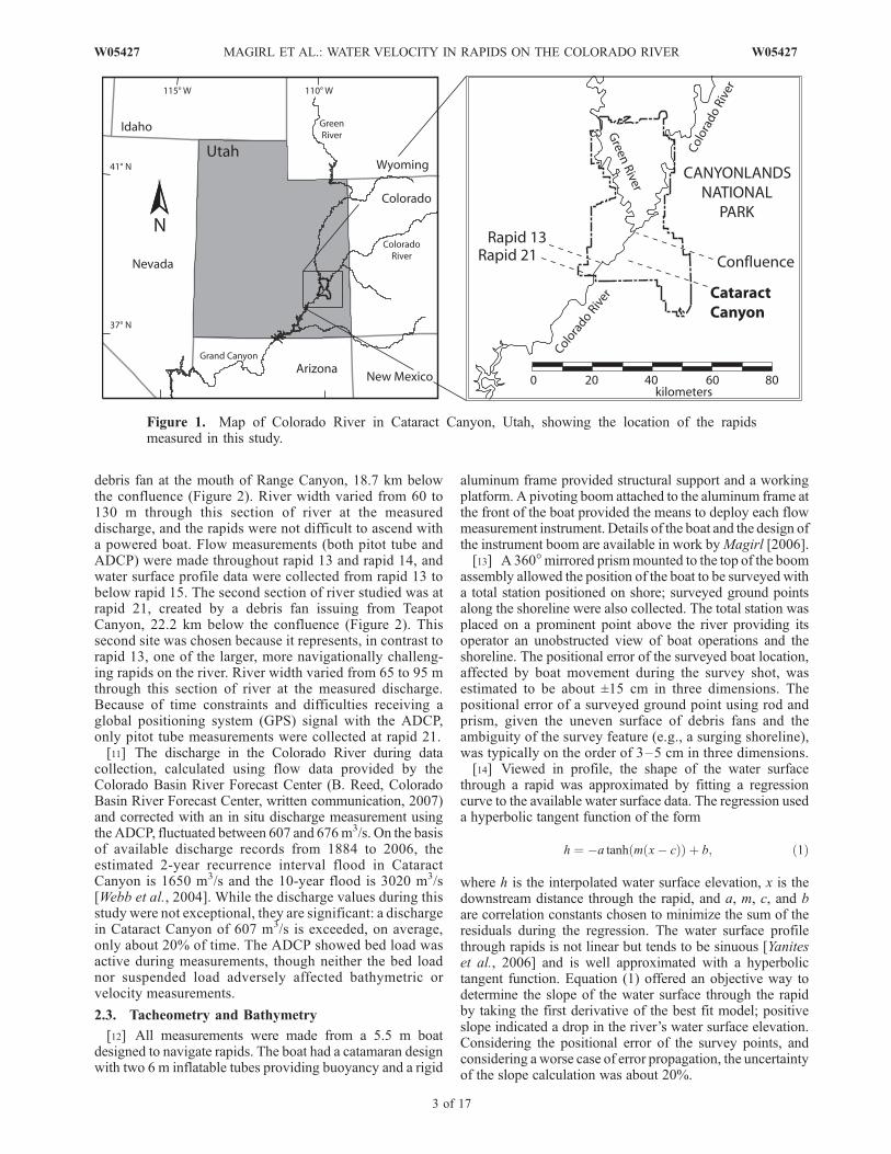
[9] Flow, water surface, and bathymetric measurementswere made in the Colorado River within Cataract Canyonfrom 23 to 26 April 2006. Cataract Canyon is withinCanyonlands National Park, just below the confluence ofthe Green and Colorado rivers in eastern Utah (Figure 1).While flow regulation from upstream damming affects theflood regime in Cataract Canyon, the Colorado River at thislocation is still subject to large spring snowmelt floods,heavy sediment load, and seasonal temperature fluctuationscharacteristic of a free-flowing river [Webb et al., 2004].Cataract Canyon, containing more than 27 extant rapidsover a 21 km reach, is popular with white-water enthusiasts.These rapids are numbered sequentially in the downstreamdirection: rapids 1 and 27 are 6.8 and 26.1 km downstreamfrom the confluence, respectively [Belknap et al., 2006][10] Two sections of river were measured and analyzed in

detail for this study. The first section consists of a series ofclosely spaced rapids starting with rapid 13, formed by a

2 of 17

W05427 MAGIRL ET AL.: WATER VELOCITY IN RAPIDS ON THE COLORADO RIVER W05427

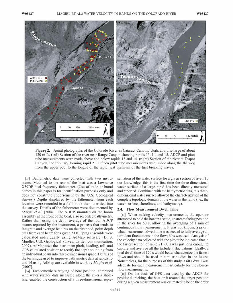
debris fan at the mouth of Range Canyon, 18.7 km belowthe confluence (Figure 2). River width varied from 60 to130 m through this section of river at the measureddischarge, and the rapids were not difficult to ascend witha powered boat. Flow measurements (both pitot tube andADCP) were made throughout rapid 13 and rapid 14, andwater surface profile data were collected from rapid 13 tobelow rapid 15. The second section of river studied was atrapid 21, created by a debris fan issuing from TeapotCanyon, 22.2 km below the confluence (Figure 2). Thissecond site was chosen because it represents, in contrast torapid 13, one of the larger, more navigationally challeng-ing rapids on the river. River width varied from 65 to 95 mthrough this section of river at the measured discharge.Because of time constraints and difficulties receiving aglobal positioning system (GPS) signal with the ADCP,only pitot tube measurements were collected at rapid 21.[11] The discharge in the Colorado River during data

collection, calculated using flow data provided by theColorado Basin River Forecast Center (B. Reed, ColoradoBasin River Forecast Center, written communication, 2007)and corrected with an in situ discharge measurement usingthe ADCP, fluctuated between 607 and 676m3/s. On the basisof available discharge records from 1884 to 2006, theestimated 2-year recurrence interval flood in CataractCanyon is 1650 m3/s and the 10-year flood is 3020 m3/s[Webb et al., 2004]. While the discharge values during thisstudy were not exceptional, they are significant: a dischargein Cataract Canyon of 607 m3/s is exceeded, on average,only about 20% of time. The ADCP showed bed load wasactive during measurements, though neither the bed loadnor suspended load adversely affected bathymetric orvelocity measurements.

2.3. Tacheometry and Bathymetry

[12] All measurements were made from a 5.5 m boatdesigned to navigate rapids. The boat had a catamaran designwith two 6 m inflatable tubes providing buoyancy and a rigid

aluminum frame provided structural support and a workingplatform. A pivoting boom attached to the aluminum frame atthe front of the boat provided the means to deploy each flowmeasurement instrument. Details of the boat and the design ofthe instrument boom are available in work byMagirl [2006].[13] A 360�mirrored prismmounted to the top of the boom

assembly allowed the position of the boat to be surveyed witha total station positioned on shore; surveyed ground pointsalong the shoreline were also collected. The total station wasplaced on a prominent point above the river providing itsoperator an unobstructed view of boat operations and theshoreline. The positional error of the surveyed boat location,affected by boat movement during the survey shot, wasestimated to be about ±15 cm in three dimensions. Thepositional error of a surveyed ground point using rod andprism, given the uneven surface of debris fans and theambiguity of the survey feature (e.g., a surging shoreline),was typically on the order of 3–5 cm in three dimensions.[14] Viewed in profile, the shape of the water surface

through a rapid was approximated by fitting a regressioncurve to the available water surface data. The regression useda hyperbolic tangent function of the form

h ¼ �a tanh m x� cð Þð Þ þ b; ð1Þ

where h is the interpolated water surface elevation, x is thedownstream distance through the rapid, and a, m, c, and bare correlation constants chosen to minimize the sum of theresiduals during the regression. The water surface profilethrough rapids is not linear but tends to be sinuous [Yaniteset al., 2006] and is well approximated with a hyperbolictangent function. Equation (1) offered an objective way todetermine the slope of the water surface through the rapidby taking the first derivative of the best fit model; positiveslope indicated a drop in the river’s water surface elevation.Considering the positional error of the survey points, andconsidering a worse case of error propagation, the uncertaintyof the slope calculation was about 20%.

Figure 1. Map of Colorado River in Cataract Canyon, Utah, showing the location of the rapidsmeasured in this study.

W05427 MAGIRL ET AL.: WATER VELOCITY IN RAPIDS ON THE COLORADO RIVER

3 of 17

W05427

[15] Bathymetric data were collected with two instru-ments. Mounted to the rear of the boat was a LowranceX59DF dual-frequency fathometer. (Use of trade or brandnames in this paper is for identification purposes only anddoes not constitute endorsement by the U.S. GeologicalSurvey.) Depths displayed by the fathometer from eachlocation were recorded in a field book then later tied intothe survey. Details of the fathometer were documented byMagirl et al. [2006]. The ADCP, mounted on the boomassembly at the front of the boat, also recorded bathymetry.Rather than using the depth average of the four ADCPbeams reported by the instrument, a process that tends tointegrate and average features on the river bed, point depthdata from each beam for a given ADCP ping ensemble werecalculated individually using AdMap software (D. S.Mueller, U.S. Geological Survey, written communication,2007). AdMap uses the instrument pitch, heading, roll, andGPS-calculated position to rectify the depth sounding froman individual beam into three-dimensional space. Details ofthe technique used to improve bathymetric data at rapids 13and 14 using AdMap are available in work by Magirl et al.[2007].[16] Tacheometric surveying of boat position, combined

with water surface data measured along the river’s shore-line, enabled the construction of a three-dimensional repre-

sentation of the water surface for a given section of river. Toour knowledge, this is the first time the three-dimensionalwater surface of a large rapid has been directly measuredand reported. Combined with the bathymetric data, this three-dimensional water surface allowed the characterization of thecomplete topologic domain of the water in the rapid (i.e., thewater surface, shorelines, and bathymetry).

2.4. Flow Measurement Dwell Time

[17] When making velocity measurements, the operatorattempted to hold the boat in a static, upstream facing positionin the river for 60 s, allowing the averaging of 1 min ofcontinuous flow measurements. It was not known, a priori,what measurement dwell time was needed to fully average allturbulent fluctuations in the flow; 60 s was used. Analysis ofthe velocity data collected with the pitot tube indicated that inthe fastest section of rapid 21, 60 s was just long enough tocapture and average all the turbulent fluctuations. Ideally, atotal dwell time of 120 s would better characterize the fastestflows and should be used in similar studies in the future.Nonetheless, for the purposes of this study, a 60 s dwell wasadequate for each measurement, particularly for the slower-flow measurements.[18] On the basis of GPS data used by the ADCP for

positional tracking, the boat drift around the target positionduring a given measurement was estimated to be on the order

Figure 2. Aerial photographs of the Colorado River in Cataract Canyon, Utah, at a discharge of about120 m3/s. (left) Section of the river near Range Canyon showing rapids 13, 14, and 15. ADCP and pitottube measurements were made above and below rapids 13 and 14. (right) Section of the river at TeapotCanyon, the tributary forming rapid 21. Fifteen pitot tube measurements were made along the thalwegfrom the upper pool to the tongue of the rapid, just upstream of the first breaking waves.

4 of 17


of ±5 m (horizontally) in the fastest, most turbulent sectionsof the river. Therefore, the velocity data collected with eachinstrument could have come from locations in the river up to5 m away from the surveyed boat location. This positionalaccuracy of the flow measurement location improved inslower water.

2.5. Flow Instrumentation

[19] The electronic pitot-static tube used in the study wasdesigned and built at New Zealand’s National Institute ofWater and Atmospheric Research. This instrument has dy-namic and static pressure sensing ports similar to aircraftairspeed and altitude sensors. The pitot tube is mounted at thefront of a streamlined ‘‘torpedo’’ to reduce vibration of thepressure sensors. The dynamic pressure port at the tip ofthe tube is 3 mm in diameter. The static pressure sensingport comprises a ring of eight 1 mm holes equally spacedaround the 16 mm diameter shaft of the pitot tube. Static anddynamic pressures are measured with Motorola MPX100series transducers with ±0.25% linearity and response timeof 1 � 10�3 s. Measuring the difference between theoncoming flow’s stagnation pressure and static pressureallows Bernoulli’s principle [Fox and McDonald, 1985] tobe used to estimate the scalar component of the free-streamvelocity. The instrument was designed to measure flowvelocity up to 9 m/s.[20] The pitot tube measures pressure which is directly

proportional to velocity head,

u2i2g

; ð2Þ

where ui is the instantaneous velocity measurement and g isthe gravitational constant. A high sampling frequency isrequired to correctly calculate mean velocity in turbulent

flow, where ui 6¼ffiffiffiffiffiu2i

q. The instrument sampling frequency

(28 Hz) enabled the pitot tube to measure even the smallestturbulent fluctuations within the flow [Smart, 1999]. Unliketurbulence measurements with an acoustic Doppler veloci-meter [Lane et al., 1998], the pitot tube required no signalprocessing or active filtering of the output signal becausethe pitot tube directly measured the pressure fluctuations inthe flow.[21] The electronic pitot tube was mounted 0.39 m below

the water surface and attached to the end of the boomassembly with a pivoting steel rod. Deeper measurements inthe water column were not attempted out of safety concernsfor the crew and instrument. The pivot of the rod (roughly±15� around an axis parallel to the boom rotation axis)allowed the streamlined pitot tube to self-adjust its angle ofattack to the oncoming flow, thus more accurately quanti-fying the scalar component of oncoming flow. Velocitycomponents orthogonal to the axis of the pitot tube, frominstrument misalignment or turbulent eddies sweeping pastthe instrument ports, have the potential to induce measure-ment error. Ackerman and Hoover [2001], however, foundvelocity measurements were reasonably consistent for apitot-static tube oriented at angle of attacks up to ±20�.The magnitude of error from orthogonal velocity compo-nents in the flow was not evaluated for this study, thoughthis error source was probably small.

[22] The ADCP, a Teledyne RD Instruments 600 kHzWorkHorse unit with a Trimble AG132 differential GPS, wasused to measure water velocity profiles. The ADCP’s theoryof operation is well documented [e.g., RDInstruments, 1996;Yorke and Oberg, 2002; J. W. Gartner and N. K. Ganju, Apreliminary evaluation of near-transducer velocities collectedwith low-blank acoustic Doppler current profiler, paperpresented at Hydraulic Measurements and ExperimentalMethods 2002, American Society of Civil Engineers, EstesPark, Colorado, 28 July to 1 August 2002]. ADCPs deter-mine water current velocity by emitting sound waves, orpings, at known frequency and measuring the Doppler shiftof the returning sound waves reflected from particles sus-pended in the moving water. Using an array of four acoustictransducers oriented 90� apart and 20� from the vertical(Janus configuration), and by range gating the acousticreturns, the ADCP calculates the magnitude and directionof water moving at discrete depths or bins. Separate bottom-track pings are also used to sound bathymetric depth.[23] The ADCP was set to sample using water mode 1

[RDInstruments, 1996] with a 0.25 m blank distance and0.50m bin size. Water mode 1 is robust, designed to operate inflows with high shear, turbulence, and velocity up to 10 m/s.For this study, two water profile pings and three bottom-trackpings were selected to make up a measurement ensemble. Anensemble represents the averaging of multiple pings todetermine both velocity and water depth. The sampling ratefor an ensemble was approximately 1 Hz.[24] In calculating velocity, an ADCP assumes the flow in

the water column is homogeneous at a given bin (height) inthe water column. This assumption may lead to errors whenmeasuring potentially three-dimensional flow structureswithin the rapid.[25] Also, the high velocity, aeration, and extreme turbu-

lence in the rapid required a relatively deep ADCP placementof 0.69 m below the water surface. Even with this instrumentdepth, some ensembles were missing, particularly in fast orturbulent regions of the river. Data losses, caused by atten-uation of signal due to suspended sediment, loss of instru-ment bottom track, low signal correlation, air bubblesentrained in the flow under the instrument, or perhaps trappedair bubbles on the transducers, were probably the source ofmost ADCP reliability issues. The percentage of missingensembles was reported as a proxy for relative instrumenteffectiveness at a particular location.[26] Deeper placement of the ADCP, however, meant the

instrument would not measure velocity within one meter ofthe surface. Having no other options while working withADCP data, the water velocity within one meter of the sur-face was estimated to be equivalent to the velocity measuredin the top bin, an assumption later shown to potentiallyinvalid in the faster sections of the rapid. Nevertheless, inlieu of having no other available information, it was the bestassumption available.[27] Another issue with working in bedrock canyons was

the problematic reception of the GPS receiver, which wasneeded when moving-bed conditions created measurementbias for the ADCP using bottom tracking. For example, noADCP data were collected at rapid 21 because of insuffi-cient GPS coverage. Fortunately, the GPS did work longenough in the canyon setting at rapids 13 and 14 to provideuseful data.


5 of 17

W05427

2.6. Froude Number

[28] Froude number, Fr, compares inertial and gravita-tional forces within a flow. As long as vertical velocities aresmall and the pressure distribution is hydrostatic, it is theratio of water velocity to the propagation velocity of ashallow water wave. Froude number is typically calculatedwith velocity averaged throughout the cross section [e.g.,Chow, 1959]. Because of the nature of the flowmeasurementscollected in this study, local Fr was calculated using theapproach outlined by Liggett [1993] using shallow-watertheory,

Fr ¼ uffiffiffiffiffiffiffiffiffiffiffiffiffiffigh

�b

s ; ð3Þ

where u is depth-integrated velocity. The total depth offlow is given by h. The nonuniform velocity distributioncoefficient, b, is given by

b ¼

Z h

0

u2dz

u2h: ð4Þ

Velocity, u(z), is a function of height above the bed of theriver as measured with the ADCP. An important assumptionbehind the derivation of equation (3) is that the flow has ahydrostatic pressure distribution with negligible verticalaccelerations. In highly three-dimensional flow, or in flowwith a deformed free surface and significant verticalvelocities, equation (3) is not applicable and the usualdefinition of Fr is called into question.[29] In the absence of velocity profile data (e.g., ADCP-

collected velocity data from the entire water column), Frcan be estimated if near-surface velocity and water depth areknown. An assumption is made that the depth-integratedmean velocity in the water column is 85% of the surfacevelocity, us [Rantz et al., 1982; Costa et al., 2000]. This is areasonable assumption if the velocity profile is logarithmic.Assuming a value of b, Fr can then be estimated as follows:

Fr ¼ 0:85usffiffiffiffiffiffiffiffiffiffiffiffiffiffigh

�b

s : ð5Þ

In an attempt to confirm the validity of the Fr calculationsobtained by equations (3) and (5), a simplified approach tocalculating Fr was also applied. If flow in a rapid wasapproximately one dimensional, then detailed bathymetricdata measured during the study could be used to estimate Fr.According to Henderson [1966, p. 51], Fr in an irregular,low-gradient channel with steady, one-dimensional flow isgiven by

Fr ¼

ffiffiffiffiffiffiffiffiffiQ2B

gA3

s; ð6Þ

where Q is discharge, B is the top width of the water surface,and A is the cross-sectional area of the flowing water. While

the high-velocity, three-dimensional flow conditions withinrapids makes the application of equation (6) inappropriate ingeneral, the equation can be used as a first-order check of thevalidity of Fr as calculated with equations (3) and (5). Bysetting Fr = 1, equation (6) can also be used to calculatecritical depth of given cross section for a known discharge. Ifthe critical depth falls below the measured depth in the river,the flow is subcritical. Inversely, if the critical depth liesabove the measured depth, flow is supercritical. Schmidt[1990] used the approach of equation (6) to calculate Fr inBadger Rapid in Grand Canyon.

3. Results and Discussion

3.1. Water Surface Profile and Bathymetry

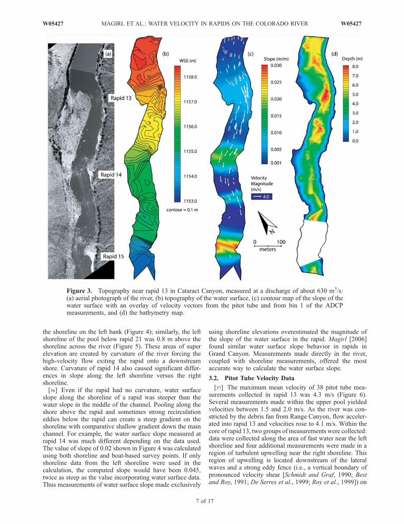
[30] A topographic map of rapids 13, 14, and 15 wasassembled using 101 water surface elevation points collect-ed during flow measurements and 82 survey points from thewater’s edge (Figure 3b). The slope of the water surface,calculated using equation (1), shows the relatively low-gradient drop in rapid 13, the steeper gradient of rapid 14,and the relatively high-gradient drop of rapid 15 (Figure 3c).A secondary rapid is present between rapid 14 and rapid 15,formed by a deposit of coarse-grained sediment carried downfrom rapids 13 and 14. These secondary rapids are a commongeomorphic characteristic of rivers with fan-eddy complexes[Howard and Dolan, 1981; Webb et al., 1989; Melis et al.,1994; Grams and Schmidt, 1999].[31] The bathymetric map of rapids 13 and 14 (Figure 3d)

was assembled using over 15,000 ADCP depth measure-ments processed with AdMap software. Even in the tur-bulence of rapids, ADCP bottom pings were reliable anddid not require the averaging of multiple measurementensembles.[32] Viewed in profile, the hydraulic characteristics of

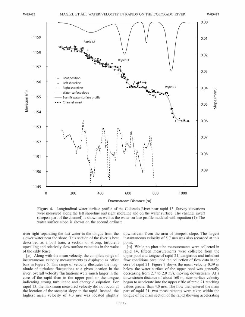
rapids 13, 14, and 15 are apparent (Figure 4). Rapid 13 wasa relatively long, low-gradient rapid with a total fall inelevation of just over 1.0 m and maximum slope of 0.006.Rapid 14 fell in elevation about 1.5 m and had a maximumslope of 0.02. In contrast, rapid 15, the largest of the threerapids in this reach, dropped about 2.0 m with a maximumslope of 0.03.[33] The channel invert is also shown in Figure 4; this

trace was constructed using the bathymetry data shown inFigure 3d. Mounds of alluvial material on the river bed thatform the rapids are apparent, and total change in elevationof the river bed along 700 m of channel from rapid 13 to justabove rapid 15 was less than 4 m affirming observations ofWebb et al. [2004] that rapids 13–18 are subsections of onecontinuous rapid.[34] The channel invert and water surface data measured

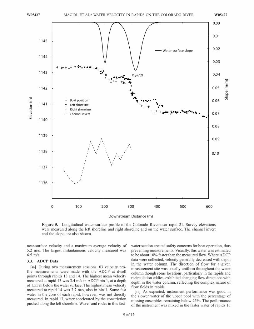
at rapid 21 are plotted in Figure 5. Rapid 21 had a smallriffle with less than 1.0 m drop just upstream of the mainrapid. The main part of rapid 21 fell over 2.0 m. The trace ofthe invert showed the collection of coarse-grained alluviumdeposited from Teapot Canyon is about 5 m below the watersurface.[35] Evident in the water surface maps are regions where

the water surface along one shoreline was noticeablydifferent from the water surface measured on the oppositeshoreline or in the center of the channel. For example, theright shoreline in the pool below rapid 14 was 0.4 m above

6 of 17


the shoreline on the left bank (Figure 4); similarly, the leftshoreline of the pool below rapid 21 was 0.8 m above theshoreline across the river (Figure 5). These areas of superelevation are created by curvature of the river forcing thehigh-velocity flow exiting the rapid onto a downstreamshore. Curvature of rapid 14 also caused significant differ-ences in slope along the left shoreline versus the rightshoreline.[36] Even if the rapid had no curvature, water surface

slope along the shoreline of a rapid was steeper than thewater slope in the middle of the channel. Pooling along theshore above the rapid and sometimes strong recirculationeddies below the rapid can create a steep gradient on theshoreline with comparative shallow gradient down the mainchannel. For example, the water surface slope measured atrapid 14 was much different depending on the data used.The value of slope of 0.02 shown in Figure 4 was calculatedusing both shoreline and boat-based survey points. If onlyshoreline data from the left shoreline were used in thecalculation, the computed slope would have been 0.045,twice as steep as the value incorporating water surface data.Thus measurements of water surface slope made exclusively

using shoreline elevations overestimated the magnitude ofthe slope of the water surface in the rapid. Magirl [2006]found similar water surface slope behavior in rapids inGrand Canyon. Measurements made directly in the river,coupled with shoreline measurements, offered the mostaccurate way to calculate the water surface slope.

3.2. Pitot Tube Velocity Data

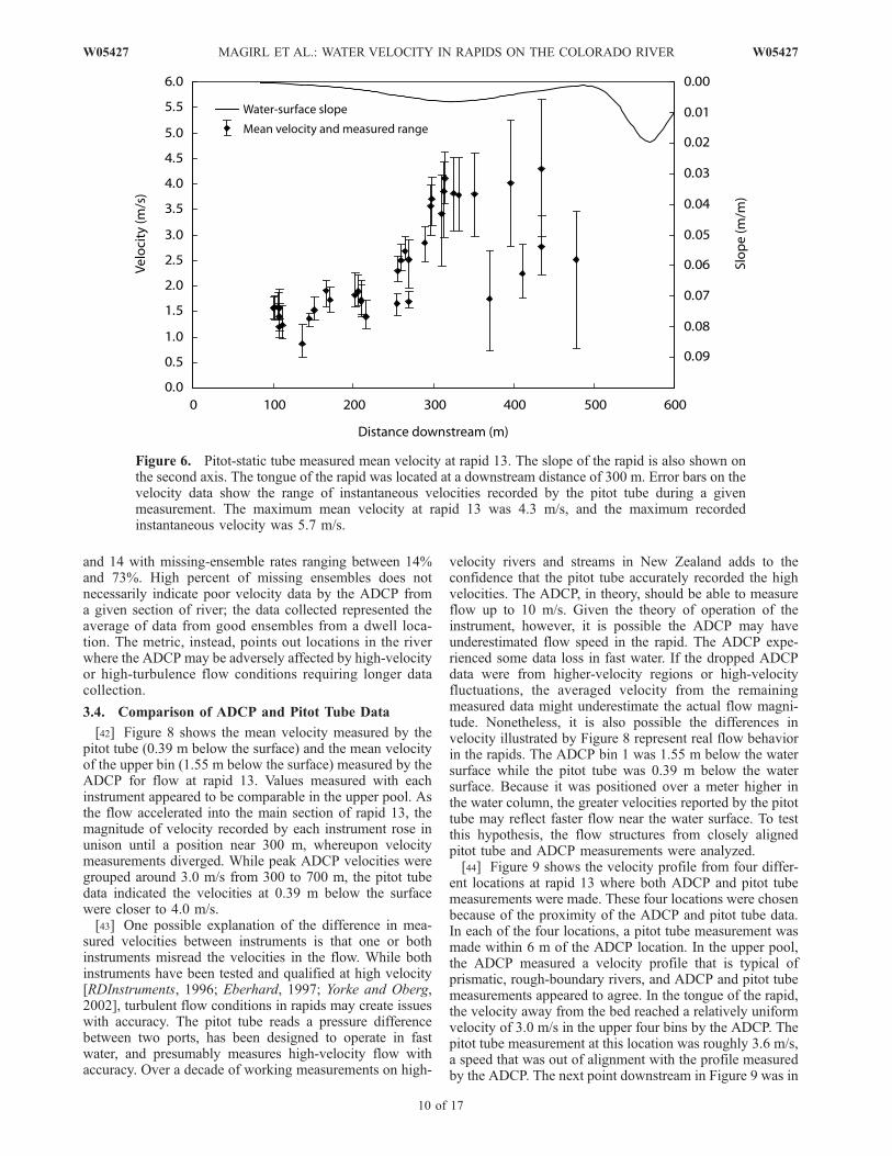
[37] The maximum mean velocity of 38 pitot tube mea-surements collected in rapid 13 was 4.3 m/s (Figure 6).Several measurements made within the upper pool yieldedvelocities between 1.5 and 2.0 m/s. As the river was con-stricted by the debris fan from Range Canyon, flow acceler-ated into rapid 13 and velocities rose to 4.1 m/s. Within thecore of rapid 13, two groups of measurements were collected:data were collected along the area of fast water near the leftshoreline and four additional measurements were made in aregion of turbulent upwelling near the right shoreline. Thisregion of upwelling is located downstream of the lateralwaves and a strong eddy fence (i.e., a vertical boundary ofpronounced velocity shear [Schmidt and Graf, 1990; Bestand Roy, 1991; De Serres et al., 1999; Roy et al., 1999]) on

Figure 3. Topography near rapid 13 in Cataract Canyon, measured at a discharge of about 630 m3/s:(a) aerial photograph of the river, (b) topography of the water surface, (c) contour map of the slope of thewater surface with an overlay of velocity vectors from the pitot tube and from bin 1 of the ADCPmeasurements, and (d) the bathymetry map.


7 of 17

W05427

river right separating the fast water in the tongue from theslower water near the shore. This section of the river is bestdescribed as a boil train, a section of strong, turbulentupwelling and relatively slow surface velocities in the wakeof the eddy fence.[38] Along with the mean velocity, the complete range of

instantaneous velocity measurements is displayed as offsetbars in Figure 6. This range of velocity illustrates the mag-nitude of turbulent fluctuations at a given location in theriver; overall velocity fluctuations were much larger in thecore of the rapid than in the upper pool or the tongueindicating strong turbulence and energy dissipation. Forrapid 13, the maximum measured velocity did not occur atthe location of the steepest slope in the rapid. Instead, thehighest mean velocity of 4.3 m/s was located slightly

downstream from the area of steepest slope. The largestinstantaneous velocity of 5.7 m/s was also recorded at thispoint.[39] While no pitot tube measurements were collected in

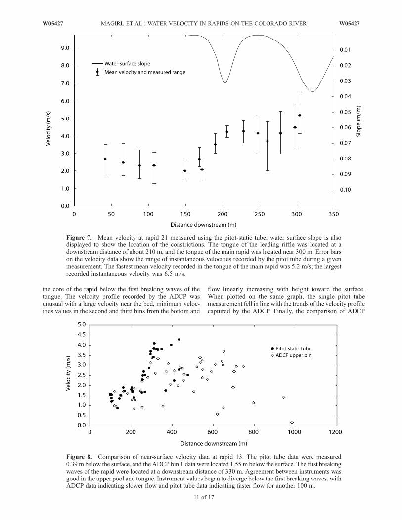
rapid 14, fifteen measurements were collected from theupper pool and tongue of rapid 21; dangerous and turbulentflow conditions precluded the collection of flow data in thecore of rapid 21. Figure 7 shows the mean velocity 0.39 mbelow the water surface of the upper pool was generallydecreasing from 2.7 to 2.0 m/s, moving downstream. At adownstream distance of about 160 m, near-surface velocitybegan to accelerate into the upper riffle of rapid 21 reachingvalues greater than 4.0 m/s. The flow then entered the mainpart of rapid 21; two measurements were taken within thetongue of the main section of the rapid showing accelerating

Figure 4. Longitudinal water surface profile of the Colorado River near rapid 13. Survey elevationswere measured along the left shoreline and right shoreline and on the water surface. The channel invert(deepest part of the channel) is shown as well as the water surface profile modeled with equation (1). Thewater surface slope is shown on the second ordinate.

8 of 17


near-surface velocity and a maximum average velocity of5.2 m/s. The largest instantaneous velocity measured was6.5 m/s.

3.3. ADCP Data

[40] During two measurement sessions, 63 velocity pro-file measurements were made with the ADCP at dwellpoints through rapids 13 and 14. The highest mean velocitymeasured at rapid 13 was 3.4 m/s in ADCP bin 1, at a depthof 1.55 m below the water surface. The highest mean velocitymeasured at rapid 14 was 3.7 m/s, also in bin 1. Some fastwater in the core of each rapid, however, was not directlymeasured. In rapid 13, water accelerated by the constrictionpushed along the left shoreline. Waves and rocks in this fast-

water section created safety concerns for boat operation, thuspreventing measurements. Visually, this water was estimatedto be about 10% faster than the measured flow.Where ADCPdata were collected, velocity generally decreased with depthin the water column. The direction of flow for a givenmeasurement site was usually uniform throughout the watercolumn though some locations, particularly in the rapids andrecirculation eddies, exhibited changing flow directions withdepth in the water column, reflecting the complex nature offlow fields in rapids.[41] As expected, instrument performance was good in

the slower water of the upper pool with the percentage ofmissing ensembles remaining below 25%. The performanceof the instrument was mixed in the faster water of rapids 13

Figure 5. Longitudinal water surface profile of the Colorado River near rapid 21. Survey elevationswere measured along the left shoreline and right shoreline and on the water surface. The channel invertand the slope are also shown.


9 of 17

W05427

and 14 with missing-ensemble rates ranging between 14%and 73%. High percent of missing ensembles does notnecessarily indicate poor velocity data by the ADCP froma given section of river; the data collected represented theaverage of data from good ensembles from a dwell loca-tion. The metric, instead, points out locations in the riverwhere the ADCP may be adversely affected by high-velocityor high-turbulence flow conditions requiring longer datacollection.

3.4. Comparison of ADCP and Pitot Tube Data

[42] Figure 8 shows the mean velocity measured by thepitot tube (0.39 m below the surface) and the mean velocityof the upper bin (1.55 m below the surface) measured by theADCP for flow at rapid 13. Values measured with eachinstrument appeared to be comparable in the upper pool. Asthe flow accelerated into the main section of rapid 13, themagnitude of velocity recorded by each instrument rose inunison until a position near 300 m, whereupon velocitymeasurements diverged. While peak ADCP velocities weregrouped around 3.0 m/s from 300 to 700 m, the pitot tubedata indicated the velocities at 0.39 m below the surfacewere closer to 4.0 m/s.[43] One possible explanation of the difference in mea-

sured velocities between instruments is that one or bothinstruments misread the velocities in the flow. While bothinstruments have been tested and qualified at high velocity[RDInstruments, 1996; Eberhard, 1997; Yorke and Oberg,2002], turbulent flow conditions in rapids may create issueswith accuracy. The pitot tube reads a pressure differencebetween two ports, has been designed to operate in fastwater, and presumably measures high-velocity flow withaccuracy. Over a decade of working measurements on high-

velocity rivers and streams in New Zealand adds to theconfidence that the pitot tube accurately recorded the highvelocities. The ADCP, in theory, should be able to measureflow up to 10 m/s. Given the theory of operation of theinstrument, however, it is possible the ADCP may haveunderestimated flow speed in the rapid. The ADCP expe-rienced some data loss in fast water. If the dropped ADCPdata were from higher-velocity regions or high-velocityfluctuations, the averaged velocity from the remainingmeasured data might underestimate the actual flow magni-tude. Nonetheless, it is also possible the differences invelocity illustrated by Figure 8 represent real flow behaviorin the rapids. The ADCP bin 1 was 1.55 m below the watersurface while the pitot tube was 0.39 m below the watersurface. Because it was positioned over a meter higher inthe water column, the greater velocities reported by the pitottube may reflect faster flow near the water surface. To testthis hypothesis, the flow structures from closely alignedpitot tube and ADCP measurements were analyzed.[44] Figure 9 shows the velocity profile from four differ-

ent locations at rapid 13 where both ADCP and pitot tubemeasurements were made. These four locations were chosenbecause of the proximity of the ADCP and pitot tube data.In each of the four locations, a pitot tube measurement wasmade within 6 m of the ADCP location. In the upper pool,the ADCP measured a velocity profile that is typical ofprismatic, rough-boundary rivers, and ADCP and pitot tubemeasurements appeared to agree. In the tongue of the rapid,the velocity away from the bed reached a relatively uniformvelocity of 3.0 m/s in the upper four bins by the ADCP. Thepitot tube measurement at this location was roughly 3.6 m/s,a speed that was out of alignment with the profile measuredby the ADCP. The next point downstream in Figure 9 was in

Figure 6. Pitot-static tube measured mean velocity at rapid 13. The slope of the rapid is also shown onthe second axis. The tongue of the rapid was located at a downstream distance of 300 m. Error bars on thevelocity data show the range of instantaneous velocities recorded by the pitot tube during a givenmeasurement. The maximum mean velocity at rapid 13 was 4.3 m/s, and the maximum recordedinstantaneous velocity was 5.7 m/s.

10 of 17


the core of the rapid below the first breaking waves of thetongue. The velocity profile recorded by the ADCP wasunusual with a large velocity near the bed, minimum veloc-ities values in the second and third bins from the bottom and

flow linearly increasing with height toward the surface.When plotted on the same graph, the single pitot tubemeasurement fell in line with the trends of the velocity profilecaptured by the ADCP. Finally, the comparison of ADCP

Figure 7. Mean velocity at rapid 21 measured using the pitot-static tube; water surface slope is alsodisplayed to show the location of the constrictions. The tongue of the leading riffle was located at adownstream distance of about 210 m, and the tongue of the main rapid was located near 300 m. Error barson the velocity data show the range of instantaneous velocities recorded by the pitot tube during a givenmeasurement. The fastest mean velocity recorded in the tongue of the main rapid was 5.2 m/s; the largestrecorded instantaneous velocity was 6.5 m/s.

Figure 8. Comparison of near-surface velocity data at rapid 13. The pitot tube data were measured0.39 m below the surface, and the ADCP bin 1 data were located 1.55 m below the surface. The first breakingwaves of the rapid were located at a downstream distance of 330 m. Agreement between instruments wasgood in the upper pool and tongue. Instrument values began to diverge below the first breaking waves, withADCP data indicating slower flow and pitot tube data indicating faster flow for another 100 m.


11 of 17

W05427

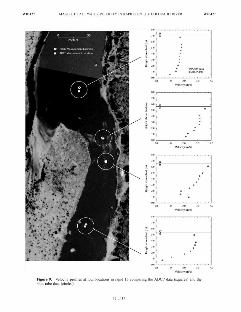
Figure 9. Velocity profiles at four locations in rapid 13 comparing the ADCP data (squares) and thepitot tube data (circles).

12 of 17


data and the pitot tube measurement in the tailwaves belowthe rapid indicated good alignment between the two data sets.The data in Figure 9 seem to suggest both instruments weremeasuring real flow behavior in the rapid in a complimentaryfashion. More importantly, within the core of the rapid, thedata suggest the highest velocity occurred near the watersurface. Tinkler [1997] observed similar velocity profiles innear-critical flow conditions and suggested that in high-gradient, rough rivers, the upper part of the water profilecan shear over the lower part of the profile.

3.5. Froude Number

[45] ADCP and bathymetry data collected at rapids 13 and14 permitted calculation of Frwith equation (3). The efficacyof applying equation (5) was also evaluated at rapid 13 usingavailable data from all instruments. At rapid 21, ADCP datawere not collected and Fr was calculated with equation (5)using pitot tube data measured near the water surface anddepths collected with the fathometer.[46] Plotted in Figure 10 with water surface slope to

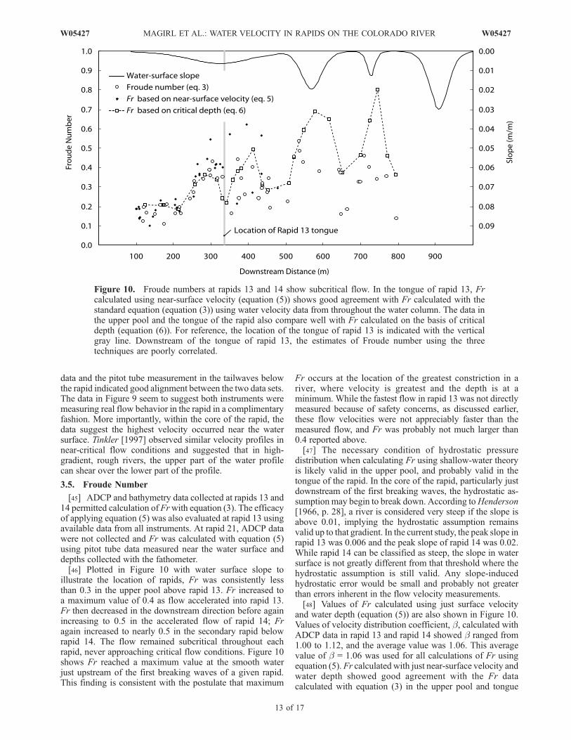
illustrate the location of rapids, Fr was consistently lessthan 0.3 in the upper pool above rapid 13. Fr increased toa maximum value of 0.4 as flow accelerated into rapid 13.Fr then decreased in the downstream direction before againincreasing to 0.5 in the accelerated flow of rapid 14; Fragain increased to nearly 0.5 in the secondary rapid belowrapid 14. The flow remained subcritical throughout eachrapid, never approaching critical flow conditions. Figure 10shows Fr reached a maximum value at the smooth waterjust upstream of the first breaking waves of a given rapid.This finding is consistent with the postulate that maximum

Fr occurs at the location of the greatest constriction in ariver, where velocity is greatest and the depth is at aminimum. While the fastest flow in rapid 13 was not directlymeasured because of safety concerns, as discussed earlier,these flow velocities were not appreciably faster than themeasured flow, and Fr was probably not much larger than0.4 reported above.[47] The necessary condition of hydrostatic pressure

distribution when calculating Fr using shallow-water theoryis likely valid in the upper pool, and probably valid in thetongue of the rapid. In the core of the rapid, particularly justdownstream of the first breaking waves, the hydrostatic as-sumption may begin to break down. According toHenderson[1966, p. 28], a river is considered very steep if the slope isabove 0.01, implying the hydrostatic assumption remainsvalid up to that gradient. In the current study, the peak slope inrapid 13 was 0.006 and the peak slope of rapid 14 was 0.02.While rapid 14 can be classified as steep, the slope in watersurface is not greatly different from that threshold where thehydrostatic assumption is still valid. Any slope-inducedhydrostatic error would be small and probably not greaterthan errors inherent in the flow velocity measurements.[48] Values of Fr calculated using just surface velocity

and water depth (equation (5)) are also shown in Figure 10.Values of velocity distribution coefficient, b, calculated withADCP data in rapid 13 and rapid 14 showed b ranged from1.00 to 1.12, and the average value was 1.06. This averagevalue of b = 1.06 was used for all calculations of Fr usingequation (5). Fr calculated with just near-surface velocity andwater depth showed good agreement with the Fr datacalculated with equation (3) in the upper pool and tongue

Figure 10. Froude numbers at rapids 13 and 14 show subcritical flow. In the tongue of rapid 13, Frcalculated using near-surface velocity (equation (5)) shows good agreement with Fr calculated with thestandard equation (equation (3)) using water velocity data from throughout the water column. The data inthe upper pool and the tongue of the rapid also compare well with Fr calculated on the basis of criticaldepth (equation (6)). For reference, the location of the tongue of rapid 13 is indicated with the verticalgray line. Downstream of the tongue of rapid 13, the estimates of Froude number using the threetechniques are poorly correlated.


13 of 17

W05427

of the rapid. Estimates of Fr from equation (5) in the core ofthe rapid, downstream of the first breaking waves, divergedfrom the value of Fr from equation (3). The higher velocitymeasured with the pitot tube near the water surface, causedthese elevated values of Fr. Equation (5) overestimates Fr inthe core of the rapid downstream from the first breakingwaves and should not be used in the core of the rapid owing tothe high surface velocity relative to mean velocity at depth.[49] Another potential error source in calculating Fr with

equation (3) and ADCP data alone is the inability of theADCP to measure surface velocity directly. The top bin of theADCP measurements was 1.55 m below the water surfaceand data in this study indicated velocity at the surface couldbe greater than velocity at 1.55 m depth, particularly in thecore of a rapid. Therefore, Fr calculations in the core of therapid using ADCP data may tend to underestimate actual Fr,though this error is probably less than 10% and decreases indeeper flow where more ADCP data can be collected.[50] To test the validity of the values of Fr calculated

with depth-integrated velocity and near-surface velocity (i.e.,equations (3) and (5)) for rapid 13, Fr was also calculatedusing the one-dimensional approach of equation (6). Thisequation is not a true calculation of Fr at a given point andcould differ significantly from the true values calculated withequation (3), but the equation does offer, using unique dataof bathymetry and not flow velocity, a rough estimate of whatFr should be in any section of the river. This techniquewas applied to the section of the river leading into rapid 13(Figure 10). Froude number calculated using equation (6)agreed well with the Fr data calculated using velocity bothin the pool above the rapid and in the section of greatestconstriction located at a downstream distance of about 280m.The Fr at 280 m, using equation (6), was calculated to be0.37. More telling, the critical depth of flow at this locationwas calculated to be 3.5 m while the actual flow depth in theriver at the time of measurement was 5.5 m. Farther down-stream, the critical depth gets closer to the true water surface,exemplified by the gradually rising Fr, but all flow in thechannel remains subcritical. Similarly, Schmidt [1990], using

the approach of equation (6) and bathymetric data fromBadger Rapid (a sizable rapid on the Colorado River inGrand Canyon), reported a maximum Fr = 0.6.[51] Froude numbers at rapid 21, calculated with

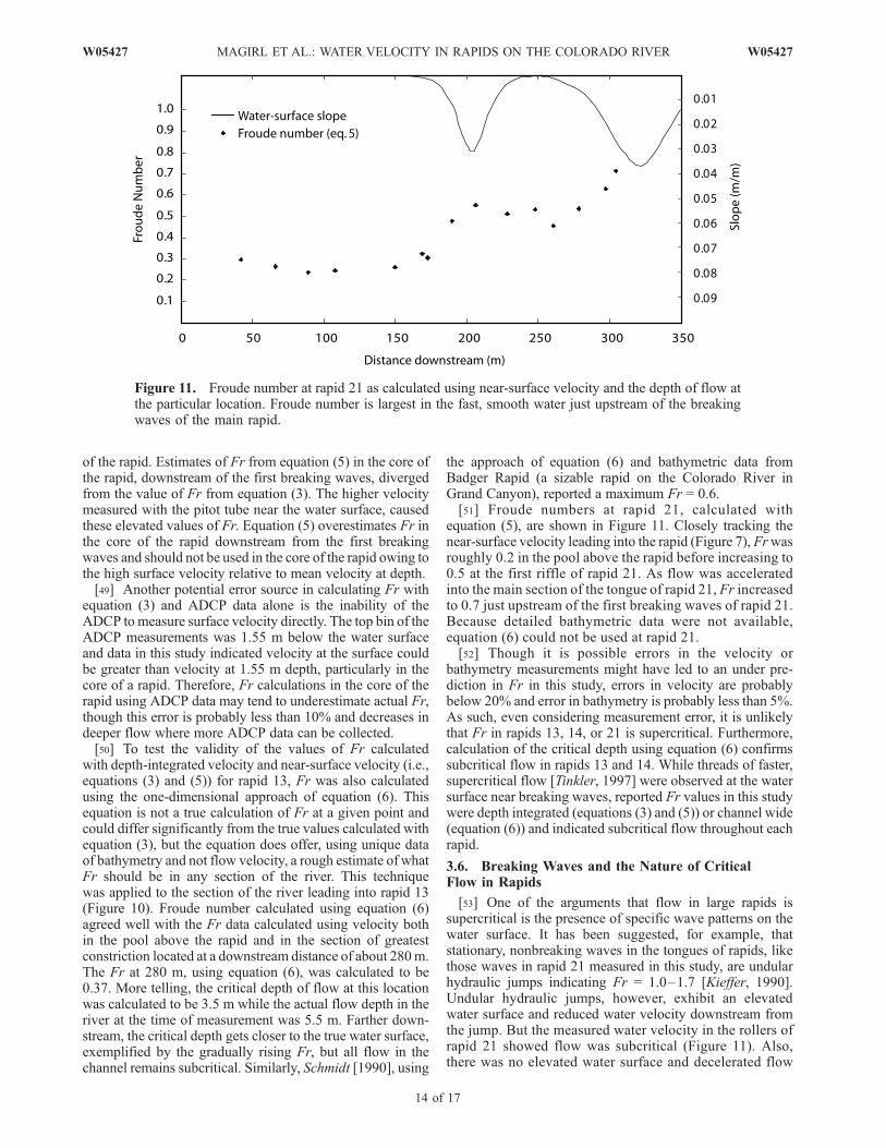
equation (5), are shown in Figure 11. Closely tracking thenear-surface velocity leading into the rapid (Figure 7), Frwasroughly 0.2 in the pool above the rapid before increasing to0.5 at the first riffle of rapid 21. As flow was acceleratedinto the main section of the tongue of rapid 21, Fr increasedto 0.7 just upstream of the first breaking waves of rapid 21.Because detailed bathymetric data were not available,equation (6) could not be used at rapid 21.[52] Though it is possible errors in the velocity or

bathymetry measurements might have led to an under pre-diction in Fr in this study, errors in velocity are probablybelow 20% and error in bathymetry is probably less than 5%.As such, even considering measurement error, it is unlikelythat Fr in rapids 13, 14, or 21 is supercritical. Furthermore,calculation of the critical depth using equation (6) confirmssubcritical flow in rapids 13 and 14. While threads of faster,supercritical flow [Tinkler, 1997] were observed at the watersurface near breaking waves, reported Fr values in this studywere depth integrated (equations (3) and (5)) or channel wide(equation (6)) and indicated subcritical flow throughout eachrapid.

3.6. Breaking Waves and the Nature of CriticalFlow in Rapids

[53] One of the arguments that flow in large rapids issupercritical is the presence of specific wave patterns on thewater surface. It has been suggested, for example, thatstationary, nonbreaking waves in the tongues of rapids, likethose waves in rapid 21 measured in this study, are undularhydraulic jumps indicating Fr = 1.0–1.7 [Kieffer, 1990].Undular hydraulic jumps, however, exhibit an elevatedwater surface and reduced water velocity downstream fromthe jump. But the measured water velocity in the rollers ofrapid 21 showed flow was subcritical (Figure 11). Also,there was no elevated water surface and decelerated flow

Figure 11. Froude number at rapid 21 as calculated using near-surface velocity and the depth of flow atthe particular location. Froude number is largest in the fast, smooth water just upstream of the breakingwaves of the main rapid.

14 of 17


downstream of the rollers indicative of an undular hydraulicjump. Rollers in the tongue of rapids are not undular jumps,instead, they are standing waves produced in near-criticalflow by depth perturbations on the bed of the channel [seeHenderson, 1966, p. 45].[54] Similarly, breaking normal waves in the Colorado

River have been taken as evidence of supercritical flow.Fundamentally, a breaking wave indicates that the distur-bance creating the wave results in wave propagation speedless than the surface velocity entering the wave (i.e., Fr, theratio of inertial to gravitational forces, is larger than 1.0).Thus, the wave breaks upon itself to maintain the waveposition within the flow. On the basis of the work of hydraulicjumps for one-dimensional flow in flumes, waves begin tobreak at Fr of about 2 [see Henderson, 1966, pp. 215–218].A direct comparison of flume studies with the highly turbu-lent and broken surface of the larger waves found in rapidssuggests Fr could be as large as 3–9 at the water surface [seealso Chow, 1959, p. 395]. But breaking normal waves inrapids, while indicating localized surface conditions of super-critical flow [Tinkler, 1997], do not necessarily point tosupercritical flow throughout the water column or acrossthe expanse of the channel. Consistent with the findings ofTinkler [1997], the results of this study show these regions ofbreaking waves, or threads of supercritical flow, are confinedto narrow, shallow sections near the water surface. When theentire depth of the channel is integrated into Fr calculation, itbecomes apparent that flow in rapids is critical or subcritical.As discharge increases, assuming the rapid does not drownout, the spatial extent of depth-integrated critical flow canexpand [Tinkler, 1997], but depth-integrated flow in rapids isgenerally not supercritical, even during large floods.[55] True supercritical flow affecting the entire channel of

a river near a rapid would have hydraulic characteristicsquite different than the flow patterns observed in ColoradoRiver rapids. Debris fans create constrictions in the channelthat can force critical flow, but if flow downstream from theconstriction forming the rapid were supercritical, the stream-lines of the flow exiting the constriction would diverge to fillthe channel until a hydraulic jump spanning the width of thechannel returned the flow to subcritical. This flow behaviorhas been demonstrated in flumes [Chow, 1959; Carling,1995] and observed in bedrock channels [Carling, 1995]and is distinctly different than flow behavior observed inrapids of the Colorado River. Schmidt et al. [1993, p. 2931],who modeled a debris flow constriction and rapid in a flume,showed that in supercritical flow (Fr � 2), streamlinesdiverge downstream from the constriction before the flowexperiences a pronounced hydraulic jump. The experimentsof Schmidt et al. [1993] also showed that in transcritical flow,any hydraulic jump is confined to the constriction, consistentwith observations in actual rapids. Because the ColoradoRiver flows over coarse-grained alluvium at all rapids [Hanksand Webb, 2006], the channel adjusts to rising discharge,achieving critical flow conditions at the debris-fan constric-tions of rapids [Kieffer, 1985]. However, there is no compel-ling evidence to suggest that channel-scale flow in debris-fanrapids on the Colorado River goes supercritical, even at largedischarge. This observation is important in studies of thehydraulics and fluvial geomorphology of the Colorado Riverand its tributaries because it allows researchers and engineers

to bracket the flow conditions that could be expected, even atlarge discharge.

4. Conclusions

[56] Velocity, bathymetry, and water surface measure-ments were made in rapids on the Colorado River in CataractCanyon, Utah. These boat-based measurements offer insightinto the complicated hydraulics of rapids and help evaluatesome assumptions applied to analysis of the high-velocitywater flowing in high-gradient rivers.[57] The collection of detailed bathymetric and water

surface data near and downstream of rapid 13 showed thecomplete topographic domain of the water within theserapids. The data revealed the three-dimensional nature ofthe water surface in rapids indicating water surface elevationsalong the shoreline of a rapid can misrepresent the actualslope of the rapid in the channel. Collection of these data isalso an early step in building computational fluid dynamicmodels to simulate flow in rapids.[58] Two flow-measurement instruments, an electronic

pitot-static tube and an ADCP, were used to characterizethe flow fields in three rapids. Both instruments provedvaluable during the study, each offering unique advantagesfor collecting velocity data in the challenging conditions ofhigh-gradient rivers. The pitot tube, placed just below thewater surface, collected detailed velocity data, including therange of turbulent fluctuations in the flow. Maximum meanvelocity measured with the pitot tube was 5.2 m/s and thefastest instantaneous velocity was 6.5 m/s. The pitot tubedesign proved well suited to measurements in the high-velocity flow field of the rapid. The ADCP collected flowdata throughout much of the water column and operatedsuccessfully within fast sections of water, though some datasuggested the possibility that the ADCP may underestimatevelocity of the fastest flow. The ADCP recorded meanvelocities as high as 3.7 m/s.[59] In contrast to the flow in alluvial rivers where the

point of maximum velocity is located below the surface, itappeared the highest velocity in the core of rapids (i.e., belowthe first breaking waves) was forced to the water surface,though further work is needed to confirm or discount thisobservation. The ADCP provided valuable and reliablebathymetric data from slow and fast sections of the river.Using a new approach of preserving the depth measurementsfrom each beam in an ensemble, detailed bathymetric maps ofthe river bed were constructed.[60] Froude number calculations indicated flow was sub-

critical in the moderately sized rapids and did not exceedcritical conditions even in the large rapid. Breaking waveswere observed even though the overall channel flow condi-tions remained subcritical. For the flow conditions analyzed,the largest Frmeasured was 0.7 in the tongue of rapid 21. Thestudy indicated Fr reached a maximum at the tongue of agiven rapid, decreasing below the first breaking waves.Realistic estimates of Fr in rapids were obtained using onlynear-surface water velocity and water depth. With the Fr datafrom this current study, comparisons with flow conditions ofearlier studies in rapids led us to conclude that supercriticalflow in the rapids of the Colorado River is rare and thatchannel-scale flow conditions in rapids remain subcritical orcritical even at large discharge.


15 of 17

W05427

[61] Acknowledgments. We are indebted to Peter Griffiths fortacheometric support, Steve Young for skilled and safe navigation of theboat in the rapids, Steve Cunningham for robust engineering of the boomassembly, and Terry Kenney for collecting ADCP data in the river. JimLiggett provided insight into the specifics of critical flow and calculatingFroude number. Mike Nolan and Bill Knight provided early reviews of themanuscript, and the insightful comments from three anonymous reviewersgreatly improved the final article.

ReferencesAckerman, J. D., and T. M. Hoover (2001), Measurement of local bed shearstress in streams using a Preston-static tube, Limnol. Oceanogr., 46(8),2080–2087.

Belknap, B., B. Belknap, and L. Belknap Evans (2006),Belknap’sWaterproofCanyonlands River Guide, 75 pp., Westwater, Evergreen, Colo.

Best, J. L., and A. G. Roy (1991), Mixing-layer distortion at the confluenceof channels of different depth, Nature, 350(6317), 411–413, doi:10.1038/350411a0.

Blalock, M. E., and T. W. Sturm (1981), Minimum specific energy incompound open channel, Proc. Am. Soc. Civ. Eng., 107(6), 699–717.

Carling, P. A. (1995), Flow-separation berms downstream of a hydraulicjump in a bedrock channel, Geomorphology, 11(3), 245–253, doi:10.1016/0169-555X(94)00052-S.

Chow, V. T. (1959), Open-Channel Hydraulics, 680 pp., McGraw-Hill,New York.

Costa, J. E., K. R. Spicer, R. T. Cheng, P. Haeni, N. B. Melcher, E. M.Thurman, W. J. Plant, and W. C. Keller (2000), Measuring stream dis-charge by non-contact methods: A proof-of-concept experiment,Geophys.Res. Lett., 27(4), 553–556, doi:10.1029/1999GL006087.

De Serres, B., A. D. Roy, P. M. Biron, and J. L. Best (1999), Three-dimensional structure of flow at a confluence of river channels withdiscordant beds, Geomorphology, 26, 313–335, doi:10.1016/S0169-555X(98)00064-6.

Douglas, M. E., and P. C. Marsh (1996), Population estimates/populationmovements of Gila cypha, an endangered cyprinid fish in Grand Canyonregion of Arizona, Copeia, 1, 15–28, doi:10.2307/1446938.

Eberhard, A. (1997), POEM test certificate dated 30 October 1997/EA,Swiss Natl. Hydrol. and Geol. Surv., Bern, Switzerland.

Fox, R. W., and A. T. McDonald (1985), Introduction to Fluid Mechanics,741 pp., John Wiley, New York.

Grams, P. E., and J. C. Schmidt (1999), Geomorphology of the Green Riverin the eastern Uinta Mountains, Dinosaur National Monument, Coloradoand Utah, in Varieties of Fluvial Form, edited by A. J. Miller and A. Gupta,pp. 81–111, John Wiley, Chichester, U. K.

Grant, G. E. (1997), Critical flow constraints flow hydraulics in mobile-bedstreams: A new hypothesis, Water Resour. Res., 33(2), 349 – 358,doi:10.1029/96WR03134.

Hanks, T. C., and R. H. Webb (2006), Effects of tributary debris on thelongitudinal profile of the Colorado River in Grand Canyon, J. Geophys.Res., 111, F02020, doi:10.1029/2004JF000257.

Hazel, J. E., Jr., D. J. Topping, J. C. Schmidt, and M. Kaplinski (2006),Influence of a dam on fine-sediment storage in a canyon river, J. Geophys.Res., 111, F01025, doi:10.1029/2004JF000193.

Henderson, F.M. (1966),Open Channel Flow, 522 pp., Macmillan, NewYork.Howard, A., and R. Dolan (1981), Geomorphology of the Colorado Riverin Grand Canyon, J. Geol., 89, 269–298.

Jarrett, R. D. (1984), Hydraulics of high-gradient streams, J. Hydraul. Eng.,110(11), 1519 – 1539, doi:10.1061/(ASCE)0733-9429(1984)110:11(1519).

Kieffer, S. W. (1985), The 1983 hydraulic jump in Crystal Rapid: Implica-tions for river-running and geomorphic evolution in the Grand Canyon,J. Geol., 93, 385–406.

Kieffer, S. W. (1987), The waves and rapids of the Colorado River, GrandCanyon, U.S. Geol. Surv. Open File Rep., 87-096, 69 pp.

Kieffer, S. W. (1988), Hydraulic map of Lava Falls Rapid, Grand Canyon,Arizona, U.S. Geol. Surv. Misc. Invest. Ser. Map, I-1897-J, scale 1:1,000,1 sheet.

Kieffer, S. W. (1990), Hydraulics and geomorphology of the ColoradoRiver in the Grand Canyon, in Grand Canyon Geology, edited by S. S.Bues and M. Morales, pp. 333–383, Oxford Univ. Press, New York.

Lane, S. N., P. M. Biron, K. F. Bradbrook, J. B. Butler, J. H. Chandler,M. D. Crowell, S. J. McLelland, K. S. Richards, and A. D. Roy (1998),Three-dimensional measurement of river channel flow processes usingacoustic Doppler velocimetry, Earth Surf. Processes Landforms, 23,1247 – 1267, doi:10.1002/(SICI)1096-9837(199812)23:13<1247::AID-ESP930>3.0.CO;2-D.

Larsen, I. J., J. C. Schmidt, and J. A. Martin (2004), Debris-fan reworkingduring low-magnitude floods in the Green River canyons of the easternUinta Mountains, Colorado and Utah, Geology, 32(4), 309 – 312,doi:10.1130/G20235.1.

Leopold, L. B. (1969), The rapids and the pools—Grand Canyon, in TheColorado River Region and John Wesley Powell, U.S. Geol. Surv. Prof.Pap., 669, pp. 131–145.

Liggett, J. A. (1993), Critical depth, velocity profiles, and averaging,J. Irrig. Drain. Eng., 119(2), 416 –422, doi:10.1061/(ASCE)0733-9437(1993)119:2(416).

Loomis, J., A. J. Douglas, and D. A. Harpman (2005), Recreation usevalues and nonuse values of Glen and Grand Canyons, in The State ofthe Colorado River Ecosystem in Grand Canyon, edited by S. P. Gloss etal., pp. 153–164, U.S. Geol. Surv. Circ., 1282.

Magirl, C. S. (2006), Bedrock-controlled fluvial geomorphology and thehydraulics of rapids on the Colorado River, Ph.D. dissertation, Univ. ofAriz., Tucson.

Magirl, C. S., P. G. Griffiths, and R. H. Webb (2006), ADV point measure-ments within rapids of the Colorado River in Grand Canyon, in Examiningthe Confluence of Environmental and Water Concerns, Proceedings ofthe 2006 World Environmental and Water Resources Congress, editedby R. Graham, 10 pp., doi:10.1061/40856(200)158, Am. Soc. of Civ.Eng., Reston, Va.

Magirl, C. S, G. M. Smart, J. W. Gartner, and R. H. Webb (2007), Tech-niques and instrumentation for measuring flow in high-gradient rivers, in2007 Hydraulic Measurements & Experimental Methods Conference,edited by E. A. Cowin and D. F. Hill, pp. 454–459, Am. Soc. of Civ.Eng., Reston, Va.

Melis, T. S., R. H. Webb, P. G. Griffiths, and T. J. Wise (1994), Magnitudeand frequency data for historic debris flows in Grand Canyon NationalPark and vicinity, U.S. Geol. Surv. Water Resour. Invest. Rep., 94-4214.

Miller, A. J. (1994), Debris-fan constrictions and flood hydraulics in rivercanyons: Some implications from two-dimensional flow modeling, EarthSurf. Processes Landforms, 19(8), 681 – 697, doi:10.1002/esp.3290190803.

Nikora, V. I., and G. M. Smart (1997), Turbulence characteristics ofNew Zealand gravel-bed rivers, J. Hydraul. Eng., 123(9), 764–773,doi:10.1061/(ASCE)0733-9429(1997)123:9(764).

Parker, G., and N. Izumi (2000), Purely erosional cyclic and solitary stepscreated by flow over a cohesive bed, J. Fluid Mech., 419, 203–238,doi:10.1017/S0022112000001403.

Rantz, S. E., et al. (1982), Measurement and computation of streamflow:Volume 1, Measurement of stage and discharge, U.S. Geol. Surv. WaterSupply Pap., 2175, 284 pp.

RDInstruments (1996), Acoustic Doppler current profilers—Principles ofoperation: A practical primer, 54 pp., San Diego, Calif.

Roy, A. G., P. M. Biron, T. Buffin-Belanger, and M. Levasseur (1999), Com-bined visual and quantitative techniques in the study of turbulent flows,Water Resour. Res., 35(3), 871–877, doi:10.1029/1998WR900079.

Schmidt, J. C. (1990), Recirculating flow and sedimentation in the Color-ado River in Grand Canyon, Arizona, J. Geol., 98, 709–724.

Schmidt, J. C., and J. B. Graf (1990), Aggradation and degradation ofalluvial sand deposits, 1965–1986, Colorado River, Grand CanyonNational Park, Arizona, U.S. Geol. Surv. Prof. Pap., 1493.

Schmidt, J. C., and D. M. Rubin (1995), Regulated streamflow, fine-graineddeposits, and effective discharge in canyons with abundant debris fans, inNatural and Anthropogenic Influences in Fluvial Geomorphology, Geo-phys. Monogr. Ser., vol. 89, edited by J. E. Costa et al., pp. 177–195,AGU, Washington, D. C.

Schmidt, J. C., D. M. Rubin, and H. Ikeda (1993), Flume simulation ofrecirculating flow and sedimentation, Water Resour. Res., 29(8), 2925–2939, doi:10.1029/93WR00770.

Smart, G. M. (1994), Turbulent velocities in a mountain river, in HydraulicEngineering ’94: Proceedings of the 1994 Conference, edited by G. V.Cotroneo and R. R. Rumer, pp. 844–848, Am. Soc. of Civ. Eng., Reston, va.

Smart, G. M. (1999), Turbulent velocity profiles and boundary shear ingravel bed rivers, J. Hydraul. Eng., 125(2), 106–116, doi:10.1061/(ASCE)0733-9429(1999)125:2(106).

Stevens, L. E., J. P. Shannon, and D. W. Blinn (1997), Colorado Riverbenthic ecology in Grand Canyon, Arizona, USA: Dam, tributary andgeomorphological influences, Reg. Rivers Res. Manage., 13, 129–149,doi:10.1002/(SICI)1099-1646(199703)13:2<129::AID-RRR431>3.0.CO;2-S.

Thompson, D. M. (2007), The characteristics of turbulence in a shear zonedownstream of a channel constriction in a coarse-grained forced pool,Geomorphology, 83, 199–214, doi:10.1016/j.geomorph.2006.05.001.

16 of 17


Thompson, D. M., E. E. Wohl, and R. D. Jarrett (1999), Velocity reversalsand sediment sorting in pools and riffles controlled by channel constrictions,Geomorphology, 27, 229–241, doi:10.1016/S0169-555X(98)00082-8.

Thorne, C. R., and L. W. Zevenbergen (1985), Estimating mean velocity inmountain rivers, J. Hydraul. Eng., 111(4), 612 –624, doi:10.1061/(ASCE)0733-9429(1985)111:4(612).

Tinkler, K. J. (1997), Critical flow in rockbed streams with estimated valuesfor Manning’s n, Geomorphology, 20, 147–164, doi:10.1016/S0169-555X(97)00011-1.

Trieste, D. J. (1992), Evaluation of supercritical/subcritical flows in high-gradient channel, J. Hydraul. Eng., 118(8), 1107–1118, doi:10.1061/(ASCE)0733-9429(1992)118:8(1107).

Valle, B. L., and G. B. Pasternack (2006), Field mapping and digital eleva-tion modelling of submerged and unsubmerged hydraulic jump regions ina bedrock step-pool channel, Earth Surf. Processes Landforms, 31, 646–664, doi:10.1002/esp.1293.

Webb, R. H. (1996), Grand Canyon, a Century of Change, Univ. of Ariz.Press, Tucson, Ariz.

Webb, R. H., P. T. Pringle, and G. R. Rink (1989), Debris flows fromtributaries of the Colorado River, Grand Canyon National Park, Arizona,U.S. Geol. Surv. Prof. Pap., 1492, 39 pp.

Webb, R. H., T. S. Melis, P. G. Griffiths, and J. G. Elliot (1999), Reworkingof aggraded debris fans, in The Controlled Flood in Grand Canyon,Geophys. Monogr. Ser., vol. 110, pp. 37–51, AGU, Washington, D. C.

Webb, R. H., J. Belnap, and J. Weisheit (2004), Cataract Canyon: A Humanand Environmental History of the Rivers in Canyonlands, 268 pp., Univ. ofUtah Press, Salt Lake City, Utah.

Wilcox, A. C., and E. E.Wohl (2007), Field measurements of three-dimensionalhydraulics in a step-pool channel, Geomorphology, 83, 215 – 231,doi:10.1016/j.geomorph.2006.02.017.

Wohl, E. E., and D. M. Thompson (2000), Velocity characteristics along asmall step-pool channel, Earth Surf. Processes Landforms, 25, 353–367,doi:10.1002/(SICI)1096-9837(200004)25:4<353::AID-ESP59>3.0.CO;2-5.

Yanites, B. J., R. H. Webb, P. G. Griffiths, and C. S. Magirl (2006), Debrisflow deposition and reworking by the Colorado River in Grand Canyon,Arizona, Water Resour. Res., 42, W11411, doi:10.1029/2005WR004847.

Yorke, T. H., and K. A. Oberg (2002), Measuring river velocity and dis-charge with acoustic Doppler profilers, Flow Meas. Instrum., 13, 191–195, doi:10.1016/S0955-5986(02)00051-1.

��J. W. Gartner and R. H. Webb, U.S. Geological Survey, 520 North Park

Avenue, Tucson, AZ 85719, USA.

C. S. Magirl, U.S. Geological Survey, 934 Broadway, Suite 300, Tacoma,WA 98402, USA. ([email protected])

G. M. Smart, National Institute of Water and Atmospheric Research, Box8602, Christchurch, New Zealand.


17 of 17

W05427

Documents

Click Here Full Article Water velocity and the nature of … velocity and the nature of critical flow in large rapids on the Colorado River, Utah Christopher S. Magirl,1 Jeffrey W