Climate change and growth scenariosfor California wildfire

A. L. Westerling & B. P. Bryant & H. K. Preisler &

T. P. Holmes & H. G. Hidalgo & T. Das & S. R. Shrestha

Received: 21 September 2011 /Accepted: 17 October 2011 /Published online: 24 November 2011# Springer Science+Business Media B.V. 2011

Abstract Large wildfire occurrence and burned area are modeled using hydroclimate andlandsurface characteristics under a range of future climate and development scenarios. Therange of uncertainty for future wildfire regimes is analyzed over two emissions pathways(the Special Report on Emissions Scenarios [SRES] A2 and B1 scenarios); three globalclimate models (Centre National de Recherches Météorologiques CM3, Geophysical FluidDynamics Laboratory CM2.1 and National Center for Atmospheric Research PCM1); threescenarios for future population growth and development footprint; and two thresholds fordefining the wildland-urban interface relative to housing density. Results were assessed forthree 30-year time periods centered on 2020, 2050, and 2085, relative to a 30-year referenceperiod centered on 1975. Increases in wildfire burned area are anticipated for mostscenarios, although the range of outcomes is large and increases with time. The increase inwildfire burned area associated with the higher emissions pathway (SRES A2) issubstantial, with increases statewide ranging from 36% to 74% by 2085, and increasesexceeding 100% in much of the forested areas of Northern California in every SRES A2scenario by 2085.

Climatic Change (2011) 109 (Suppl 1):S445–S463DOI 10.1007/s10584-011-0329-9

Electronic supplementary material The online version of this article (doi:10.1007/s10584-011-0329-9)contains supplementary material, which is available to authorized users.

A. L. Westerling (*) : S. R. ShresthaUniversity of California, Merced, 5200 N. Lake Rd, Merced, CA 95343, USAe-mail: awesterling@ucmerced.edu

B. P. BryantPardee RAND Graduate School, The RAND Corporation, Santa Monica, CA, USA

H. K. PreislerUSDA Forest Service Pacific Southwest Research Station, Albany, CA, USA

T. P. HolmesUSDA Forest Service Southern Research Station, Research Triangle Park, NC, USA

H. G. HidalgoSchool of Physics and Center for Geophysical Research, University of Costa Rica, San Jose, Costa Rica

T. DasCH2MHILL, Inc., San Diego, CA 92101, USA

1 Introduction

The climate system interacts with various factors such as soils, topography, available plantspecies, and sources of ignition to give rise to both natural ecosystems and their fireregimes. Long-term patterns of temperature and precipitation determine the moistureavailable to grow the vegetation that fuels wildfires (Stephenson 1998). Climatic variabilityon interannual and shorter scales governs the flammability of these fuels (e.g., Westerling et al.2003; Heyerdahl et al. 2001; Kipfmueller and Swetnam 2000; Veblen et al. 2000; Swetnamand Betancourt 1998; Balling et al. 1992). Flammability and fire frequency in turn affect theamount and continuity of available fuels. Consequently, long-term trends in climate can haveprofound implications for the location, frequency, extent, and severity of wildfires and for thecharacter of the ecosystems that support them (Westerling 2009).

Human-induced climatic change may, over a relatively short time period (< 100 years),give rise to climates outside anything experienced in California since the establishment ofan industrial civilization currently sustaining a state population that has increasedapproximately 41,000% since 1850. Changes in wildfire regimes driven by climate changeare likely to impact ecosystem services that California citizens rely on, including carbonsequestration in California forests; quality, quantity and timing of water runoff; air quality;wildlife habitat; viewsheds and recreational opportunities. They may also impact the abilityof homeowners and federal, state, and local authorities to secure homes in the wildland-urban interface from damage by wildfires (Westerling and Bryant 2008).

In addition to climate change, the continued growth of California’s population and thespatial pattern of development that accompanies that growth are likely to directly affectwildfire regimes through their effects on the availability and continuity of fuels and theavailability of ignitions. They are also likely to impact both wildfire and property losses dueto wildfire through their effects on the extent and value of development in California’swildland-urban interface, both through their effects on the number of structures proximateto wildfire risks and their effects on fire suppression strategies and effectiveness.

The combined effects of climate change and development on California’s future largewildfire occurrence and burned area are the focus of the research presented here. Our modelingprojects California’s fire regimes as they are currently managed onto scenarios for futureclimate, population, and development. The methodology we employ can incorporate the effectsof spatial variations in current management strategies on average fire risks. However, themonthly and interannual variations in large wildfire occurrence and burned area that weestimate do not reflect changes in management strategies over time, although our modelingdoes have the capacity to reflect changes in the effectiveness of current management strategiesto the extent that these changes currently tend to correlate with climate and landsurfacecharacteristics. Thus, hypothetical effects of future changes in management in response to theimpacts of climate and development on wildfire are not considered in this work.

The metrics we model—large fire occurrence and burned area—are not the only metrics wewould wish to employ to assess the full range of the ecological and human impacts of wildfire.In particular, metrics of fire severity (e.g., the percent of available biomass consumed,characteristics of ecological impacts) would be highly desirable as well. These metrics are likelyto change in response to climate, may also be influenced by future management decisions, andare key components for estimating many wildfire impacts due to climate change. The workreported here does not consider changes in fire severity, which are the target of multiple ongoingresearch efforts. However, in interpreting our results, it would be a mistake to assume a linearcorrespondence between increased burned area and fire severity. Fire severity is likely toincrease in some ecosystems and decrease in others alongside increases in burned area.

S446 Climatic Change (2011) 109 (Suppl 1):S445–S463

Furthermore, severity might decrease in some ecosystems for reasons that many Californiaresidents would find undesirable (i.e., broad-scale changes in ecosystems).

This work extends an analysis by Westerling and Bryant (2008) that considered theeffects of climate change on California large (>200 ha) wildfire occurrence and wildfire-related damages holding development fixed at the 2000 census. In this analysis westatistically model large (>200 and >8,500 ha) wildfire occurrence as a product of bothfuture climate scenarios and future population and development scenarios, using nonlinearlogistic regression techniques developed for seasonal wildfire forecasting in California andthe western United States (Preisler and Westerling 2007). We model the expected burnedarea using Generalized Pareto Distributions fit to observed wildfires >200 and >8,500 ha.We assess a range of outcomes given numerous sources of uncertainty, including threeglobal climate models (GCMs) with different sensitivities of temperature and precipitationto anthropogenic forcing, two emissions scenarios, and three population growth anddevelopment scenarios. Our goal is not to determine one most likely outcome, but rather todefine a population of plausible outcomes, which can then be used in future work to assessthe robustness of combined adaptation and mitigation policy choices.

2 Data and methods

2.1 Domain and resolution

The spatial domain for this analysis was a 1/8-degree lat/long grid (~12 km resolution) boundedby the political boundary for the state of California. Areas of the state outside the currentcombined fire protection responsibility areas of the California Department of Forestry and FireProtection and contract counties (combined here and denoted CDF), the U.S. Department ofAgriculture’s Forest Service (USFS), and the U.S. Department of Interior’s National ParkService (NPS), Bureau of Land Management (BLM), and Bureau of Indian Affairs (BIA) wereexcluded. The result was a set of 2,267 grid cells within the State. Fire was then modeled overthis domain at monthly time-steps for historic and simulated climate scenarios.

Five time periods were used for this analysis. Coefficients for statistical wildfiremodels wereestimated using monthly, gridded, historical fire and climate data available for 1980–1999.These coefficients were then applied to gridded climate scenarios derived from GCMs, and theresults for three future climate periods—2005–2034, 2035–2064, and 2070–2099 (henceforthreferred to as 2020, 2050, and 2085) were compared to a common reference period (1961–1990, henceforth 1975) for each scenario. These comparisons used average annual fireoccurrence and burned area statistics computed for each 30-year period referenced above.

2.2 Fire history

A comprehensive wildfire history for California for 1980–19991 was assembled fromdigital fire records obtained from CDF, USFS, NPS, BLM, and BIA. The CDF recordsincluded perimeters for large fires under both direct CDF and contract counties’ fireprotection responsibility (obtained online at http://frap.cdf.ca.gov/). Federal fires were

1 Comprehensive data prior to 1980 are not available from some of these sources. Fire data after 1999 areavailable, but the hydrologic simulations forced with historic climate data used here were developed for theCalifornia Scenarios Project, of which this research is a component. These data ended in 1999, so thecommon period of overlap between the available fire history and the hydroclimatic data was 1980–1999.

Climatic Change (2011) 109 (Suppl 1):S445–S463 S447

sourced from point data records compiled from individual fire reports. The methods used incompiling these data are described in Westerling et al. (2006, online supplement) andWesterling and Bryant (2008). Westerling et al. (2002) describe in detail the federal data inthis sample and their response to climate variability.

Our wildfire history was aggregated to a 1/8-degree gridded monthly data set offrequencies of fires >200 ha in burned area and the total burned area in these large wildfires(544,080 data points=2,267 grid points × 20 years × 12 months/year). Wherever we refer tofire occurrence in the text, we are referring to the occurrence of wildfires greater than200 ha, unless otherwise specified. For federal-sourced wildfire data, fires were allocated tothe grid cell in which they were reported to have ignited. For CDF fires reported as polygonperimeters, fires were allocated to the grid cell corresponding to their centroid. Fires wereassigned to the month in which they were discovered. In many cases fires continued to burnfor additional months, but we did not have the means to apportion burned area by month.

Wildfires managed by the Fisheries and Wildlife Service (FWS), the Department ofDefense (DOD), and the Bureau of Reclamation (BOR) were not included because theywere not available with sufficient comprehensiveness and quality. The FWS and BOR landsare relatively small in area and—particularly in the case of FWS—located in areas (e.g.,California’s Central Valley) that would likely have been excluded from this analysis forother reasons. The Department of Defense lands in California are significant, similar inscale to those of NPS. We could extend our analysis spatially to DOD lands by applyingmodel coefficients estimated using other agencies’ fire histories to DOD lands, for whichwe have the explanatory variables. However, the vast majority of DOD lands in Californialie in southeastern desert areas of the state, which show negligible changes in fire risks bythe end of the twenty-first century under many, though not all, of our scenarios.

2.3 Land surface characteristics

2.3.1 Vegetation

Coarse vegetation characteristics used here were compiled from the Land Data AssimilationSystem (LDAS) for North America’s 1/8-degree gridded vegetation layers that use theUniversity of Maryland vegetation classification scheme with fractional vegetationadjustment (UMDvf) (Mitchell et al. 2004; Hansen et al. 2000) (For an analysis of howour modeling relates to the LDAS vegetation categories, see the supplemental materials.)

In our modeling, the primary variable we use from LDAS is the fraction of each grid cellthat is vegetated and not used for agriculture (V). In our model for estimating fireprobabilities, V plays an important role. In the limit of complete urbanization, it is clear thatthis variable is affected by encroaching human development, because a grid cell entirelycovered by dense population would lack any sufficiently large vegetated space in whichwildfires could exist. However, vegetation cover may be reduced by encroaching humandevelopment at intermediate scales as well, depending on how new growth is allocated. InSection 2.4 and the supplemental materials we describe how scenarios for allocatingprojected growth within a grid cell affect the vegetation fraction.

2.3.2 Topography

Topographic data on a 1/8-degree grid were also obtained from LDAS. The LDAStopographic layers are derived from the GTOPO30 Global 30 Arc Second (~1 km)Elevation Data Set (Mitchell et al. 2004; Gesch and Larson 1996; Verdin and Greenlee

S448 Climatic Change (2011) 109 (Suppl 1):S445–S463

1996). We tested mean and standard deviation of elevation, slope, and aspect as explanatoryvariables in our wildfire model specification.

2.3.3 Protection responsibility

Logistic regression techniques attempt to estimate probabilities of wildfires occurring at agiven time and location as a function of predictor variables. The predictand is alwaysvalued zero or one, and in this case most data points are zero, since fires are relatively rareoccurrences at ~12 km × monthly scales. It is important to distinguish between data pointsthat are zero because no fire occurred, and data points that are zero because the fires thatmay have occurred there are not reported by the agencies included in our sample. Thepractical effect of including in our modeling areas for which we do not have good firereports is to underestimate the probability of fire occurrence everywhere on average. Weused the fraction of each grid cell’s area covered by the protection responsibility of theagencies in our sample to estimate the area over which fires could occur.

A GIS layer of Local, State, and Federal protection responsibility areas in California wasobtained online from the CDF Fire and Resource Assessment Program (http://frap.cdf.ca.gov/).The polygons in this layer were extracted and intersected with our 1/8-degree grid to obtainthe fraction of each grid cell in Local (LRA), State (SRA), and Federal (FRA) protectionresponsibility areas. Since federal protection responsibility includes agencies excluded fromour sample, we obtained GIS layers of federal and Indian lands online from the United StatesNational Atlas (http://nationalatlas.gov/). These were also extracted and intersected with ourgrid in order to determine what fraction of the federal responsibility area in each grid cellcorresponded to the federal agencies in our sample.

Our analysis was limited to the SRA (for which we have CDF wildfire histories) andthose parts of the FRA administered by the federal agencies for which we have wildfirehistories (USFS, NPS, BLM, BIA). The LRA was excluded both because we do not havewildfire histories for those lands and because they are predominately developed for urbanand agricultural uses. We limited our analysis to grid cells with a combined protectionresponsibility (SRA, USFS, NPS, BLM, BIA) exceeding 15% of the total grid cell area.

2.4 Growth and development scenarios

We employed spatially explicit 100 m-resolution twenty-first century population growthand development scenarios based on work by Theobald (2005) and developed by the U.S.EPA (2008) as the Integrated Climate and Land Use Scenarios (ICLUS) for the UnitedStates. These scenarios incorporate assumptions about future trajectories with regards tosprawl as well as population growth rates based on the Intergovernmental Panel on ClimateChange (IPCC) Special Report on Emissions Scenarios (SRES) social, economic, anddemographic storylines, downscaled to the United States. We report results here for ICLUSscenarios with growth and sprawl that would be consistent with the global A1 and B2SRES scenarios, and an intermediate base case trajectory (Table 1). While we do not modelspatial variation in wildfire below the 1/8-degree grid threshold, we do consider effects ofassumptions about the allocation of new development below that level (see supplementalmaterials). Our scenarios for allocating development consider the effects of expanding thewildland-urban interface into areas that are currently vegetated versus siting newdevelopment in areas that are currently bare or agricultural land. For the intermediate case,we allocate new development proportionately across baseline vegetated, bare andagricultural areas. For the high growth and sprawl scenario (A2), we allocate new

Climatic Change (2011) 109 (Suppl 1):S445–S463 S449

development to vegetated areas, and for the low growth and sprawl scenario (B1) weallocate new development within bare and agricultural areas. Additionally, we use twodifferent thresholds for describing when a 100 m pixel is fully “urbanized,” such that awildfire cannot occur there: 147 and 1000 households per square kilometer (the limits usedin the ICLUS scenarios to define suburban areas).

2.5 Climate and hydrologic data

2.5.1 Historical data

A common set of gridded historical (1950–1999) climate data including maximum andminimum temperature, precipitation (PCP), radiation, and wind were designated for theSecond California Assessment (see Maurer et al. 2002; Hamlet and Lettenmaier 2005). Weused these data with LDAS vegetation and topography to drive the Variable InfiltrationCapacity (VIC) hydrologic model at a daily time step in full energy mode, generating a fullsuite of gridded hydroclimatic variables such as actual evapotranspiration (AET), soilmoisture, relative humidity (RH), surface temperature (TMP) and snow-water equivalent(SWE) (Liang et al. 1994). Because Potential Evapotranspiration (PET) was not easilyextracted from the version of the VIC model used here, we used the Penman-Monteithequation to estimate PET directly (Penman 1948; Monteith 1965). Moisture deficit (D) wasthen calculated from PET and AET (D = PET - AET).

As indicators of drought stress, we calculated the cumulative water-year moisture deficitfor each of the preceding 2 years (D01 and D02). Water year (October - September), ratherthan calendar year, moisture deficit is used because in California most of the precipitationthat affects fuel availability and flammability falls between October and April. We alsocalculated the standardized cumulative moisture deficit from October 1 through the currentmonth (CD0). The 30-year means for 1961–1990 for moisture deficit (D30), AET (AET30),PCP (PCP30), and TMP (TMP30) were also used below to analyze the spatial distributionof climate-vegetation-wildfire interactions to be represented in the wildfire modelspecification (Electronic Supplementary Material).

2.5.2 Climate scenarios

As described by Cayan et al. (2009), several GCMs and emissions scenarios were selectedfor the Second California Assessment. In this report we describe results across three models—CNRM CM3, GFDL CM2.1, NCAR PCM—and two emissions scenarios—SRES A2 (amedium-high emissions trajectory) and SRES B1 (a low emissions trajectory) comprisingsix realizations for future climate. Daily climate data from these models were downscaled tothe 1/8-degree grid using the Constructed Analogues method (see Hidalgo et al. 2008; Maurerand Hidalgo 2008). After downscaling, the VIC model was used to simulate the same suite of

Table 1 ICLUS growth and development scenarios for California

Scenario 2100 CA Population Change vs 2000 Description (identifier)

A2 81 million +154% high growth & sprawl (HIH,HIH)

Base Case 62 million +84% medium growth & sprawl (MID,MID)

B1 50 million +54% Low growth & sprawl (LOW,LOW)

S450 Climatic Change (2011) 109 (Suppl 1):S445–S463

hydrologic variables for each target time period (1975, 2020, 2050, 2085) in each climatescenario as described for the historical period (Section 2.5).

As described in Cayan et al. (2009), the models were selected for their fidelity inrepresenting historical California temperature and precipitation in particular, with appropriateseasonality. Also, the selected models were required to simulate tropical Pacific sea surfacetemperature variability consistent with observed ENSO variability, and to have appropriatespatial resolution over California for the downscaling methodologies employed here. That lefta set of six models. Daily precipitation and daily maximum and minimum temperature had tobe included in the models’ historical and projection saved sets in order to use the ConstructedAnalogs downscaling methodology, which narrowed the set to three models.

While we only use the three models downscaled with the Constructed Analogsmethodology, the larger set of six models show a consensus toward drier conditions insouthern and central California, but more scattered results in the region from Lake Shasta to thenorthernmost parts of California. An unpublished review of a larger set of 12 models showedsimilar results, increasing our confidence that the models used here are representative of what alarger set of models project for California. So while it is true that our models do not encompassthe full range of model uncertainty of the AR4, the GCMs used here appear to cover a range ofprojected temperature and precipitation that is representative of the state of the art modelingguidance for California. A possibly more relevant concern is that the estimated emissionsgrowth for 2000–2007 exceeded the most fossil fuel-intensive scenario of IntergovernmentalPanel on Climate Change (Le Quéré et al 2009). The longer this trend in emissions growthrates persists, the harder it may be to reach a future scenario like those modeled here, and themore likely it is our results may underestimate future impacts.

Each of the GCMs evidences different sensitivities to anthropogenic forcing, with theCNRM CM3 and GFDL CM2.1 models generally showing warmer temperatures than theNCAR PCM, particularly in summer. The other three models assessed by Cayan et al(2009) that are not used here were also warmer than the NCAR PCM. The GFDL CM2.1model tended to be drier than the others in both northern and southern California in mostscenarios, while CNRM CM3 was typically drier than NCAR PCM. Compared to the largerset of models, NCAR PCM is also the least dry by the end of the century under the A2scenario (Cayan et al 2009). It is not clear how significant variation in precipitation acrossthe models is, since that variation is small compared to the potential natural variability inprecipitation in the region. Notably, the tendency towards dryness across all the models ismuch more pronounced and uniform for California in the A2 emissions scenarios, whenanthropogenic forcing is higher, than for the B1 scenarios, and it seems reasonable tospeculate that the forcing is overwhelming the natural variation in the A2 scenarios.

The six climate scenarios used here encompass three separate sources of uncertainty forour modeling: the degree of anthropogenic forcing (represented by the A2 and B1emissions paths), the extent of climate system sensitivity to anthropogenic forcing (greaterin GFDL CM2.1 and CNRM CM3 than NCAR PCM), and the range of random variation inclimate across 30-year windows in six scenarios (unknowable for a sample of this size).

3 Modeling

3.1 Fire modeling

Because large wildfires are relatively rare events, statistical models for wildfire mustaggregate fire occurrence over space and/or time in order to avoid fitting a model of zeros.

Climatic Change (2011) 109 (Suppl 1):S445–S463 S451

Logistic regressions allow us to model wildfire occurrence at arbitrarily fine spatial andtemporal resolutions (limited only by the available data) while statistically aggregatingacross locations with similar characteristics. We estimated the monthly probability of large(>200 ha and >8500 ha) wildfires occurring as a function of land-surface characteristics,human population, and climate on a 1/8-degree grid using generalized linear models in R.Candidate model specifications were tested by comparing the Akaike Information Criterion(AIC) estimated for each model. The best model specification was then tested using leave-one-out cross-validation. That is, for each of the 20 years in the model estimation period, aseparate set of model coefficients were estimated using the other 19 years of data.

The climatic variables used here as predictors for fire occurrence (Table 2) were selected todescribe variation in moisture available for the growth and wetting of fuels over a range oftime scales, from long term averages over 30 years (D30, AET30), to interannual variations inthe 3 years through the current year (D01, D02), to seasonal variations and conditions at themonth a fire could potentially burn (CD0, PCP, RH, TMP). Westerling and Bryant (2008) andWesterling (2009) show that long-term climate averages can serve as a proxy for coarsevegetation and fire regime types, distinguishing between diverse fire regime responses toantecedent and concurrent climate. Preisler et al (2011), Westerling (2009) and Westerling etal. (2006) show that cumulative annual moisture deficits in the current and 1–2 precedingyears are strongly associated with variability in large wildfire occurrence, and the latter workalso links large wildfire occurrence to temperature and variations in spring snowmelt timing.Finally, relative humidity (RH) is a key component of many fire weather indices, and a goodpredictor of fuel moisture (e.g., Schlobohm and Brain 2002).

Vegetation fraction and population are indicators of burnable area, availability of human-origin ignitions, and accessibility. Other variables we tested—such as total protectionresponsibility area, and mean and standard deviation of elevation—were not included in themodel specification because they did not substantially improve model fit as measured bythe AIC. The climatic and land surface variables we selected are not independent oftopography and protection responsibility area. Federal protection responsibility and U.S.Forest Service protection responsibility area were highly significant, and may be indicativeof differences in management or resources across protected areas, or they may be proxiesfor other spatial variables such as accessibility, vegetation type, sources of ignitions, etc.

The model specification employed here for estimating fire occurrence builds on Preislerand Westerling (2007) and Westerling and Bryant (2008), and adopts methodologiespresented in Brillinger et al. (2003), and Preisler et al. (2004):

LogitðΠ200Þ ¼ b � ½1þ D30þ D01þ D02þ PCPþ X D30;AET30ð Þ� 1þ TMPþ CD0ð Þ þ P TMPð Þ þ P RHð ÞþP POPð Þ � 1þ D30ð Þ þ X Vð Þ þ FRA�

where Π200 is the probability of a fire >200 ha occurring, Logit(Π200) is the logarithm ofthe odds ratio ðΠ200=ð1�Π200ÞÞ, β is a vector of parameters estimated from the data, andX(•) and P(•) are matrices describing basis spline and polynomial transformations of thedata. The interaction terms:

X D30;AET30ð Þ � 1þ TMPþ CD0ð Þresult in estimation of a set of constants and a set of coefficients on average monthlytemperatures and cumulative moisture deficits that are associated with the distribution ofvegetation types and patterns of fire regime response to climate variability.

S452 Climatic Change (2011) 109 (Suppl 1):S445–S463

The interaction terms:

P POPð Þ � 1þ D30ð Þcapture direct effects of local population on the probability of large fire occurrence, whichvary in this specification with the average summer moisture deficit in any given location.These factors may be indicative of several effects, including ignitions, accessibility,suppression resources, and suppression strategies.

We also estimate the probability that one or more very large fires burning in excess of8,500 ha in aggregate may occur, conditional on there being at least one fire exceeding200 ha:

LogitðΠ8500 200j Þ ¼ b � 1þ RHþ Aspectþ USFS½ �

This model says that whether or not a large fire becomes a very large fire or not dependson the relative humidity, the north/south facing, and whether the fire is on Forest Serviceland or not. The latter variable might be related to management strategies, or it could simplybe that so much of the forested area of the state, especially in less accessible locations, ismanaged by the Forest Service.

The probabilities estimated in this way can be summed to get an expected number offires. For example, the number of wildfires >200 ha expected in California in a given yearis just the sum of the probabilities Π200 for each of 12 months and 2,267 grid cells. Theprobabilities can also be used to simulate fire histories, drawing [0,1] randomly frombinomial distributions with probabilities Π200 for each grid cell and month.

Table 2 Predictor variables

Variable Description >200 ha1 >8,500 ha2

D30 30-year average cumulative Oct.–Sep. moisture deficit √AET30 30-year average cumulative Oct.–Sep. actual evapotranspiration √D02 Cumulative 0ct.–Sep. moisture deficit, 2 years previous √D01 Cumulative 0ct.–Sep. moisture deficit, 1 year previous √CD0 Current water-year cumulative moisture deficit, Oct. through current

month√

PCP 2-month cumulative precipitation, through current month √RH Monthly average Relative Humidity √ √TMP Monthly average surface air Temperature √V3 Vegetation Fraction √POP Total population (2000) √FRA3 Federal protection responsibility area as percent of total area √USFS3 USFS protection responsibility area as percent of total area √Aspect4 Average north/south facing √

1 Predictors for logistic regression estimating probability of a fire exceeding 200 ha2 Predictors for logistic regression estimating probability total burned area exceeds 8,500 ha conditional onone fire having exceeded 200 ha3 Fractions are transformed using log fractionþ :002ð Þ= 1� fractionþ :002ð Þð Þ to generate a continuousvariable centered around zero4 The transformation cos pi=2þ aspect»pi=180ð Þ yields the north/south component of aspect

Climatic Change (2011) 109 (Suppl 1):S445–S463 S453

We also estimated generalized Pareto distributions (GPDs) for the logarithm of burnedarea for fires >200 ha and for fires >8,500 ha (for a discussion of methodology as it appliesto wildfire and evidence that fire size regimes are consistent with heavy-tailed Paretodistributions, see Straus et al. 1989; Malamud et al. 1998; Ricotta et al. 1999; Cumming2001; Song et al. 2001; Zhang et al. 2003; Schoenberg et al. 2003; Holmes et al. 2008).From these we estimated the expected burned area for a fire given that its area is greaterthan 200 ha and less than 8,500 ha, and the expected burned area for fires given that theyare >8,500 ha. Expected burned area in any grid cell and month is thus:

ExpectedBurnedArea ¼ Π200 � bA > 200;<8500 þΠ200 �Π8500 200j :�

� � bA >8500jwhere the probabilities Π are as above, bAj>200;<8500 is the expected burned area less than8,500 ha given that there is at least one fire greater than 200 ha, and bAj>8500 is the expectedburned area given that at least 8,500 ha burned.

We use a two-step process like this because the empirical distribution of fire sizes inCalifornia appears to be non-stationary. Extremely large fires are governed by differentprocesses than are more frequent large fires. As with the logistic regression results above,we can also draw randomly from the GPDs to simulate fire histories, generating a randomburned area for each fire simulated with the binomial distributions.

3.2 Summary of scenarios

To summarize, we estimate 108 future scenarios, considering two emissions scenarios, threeGCMs, two thresholds for defining urbanization, three scenarios for growth rates and theallocation of development, and three future time periods (Table 3).

4 Results and discussion

4.1 Model fit

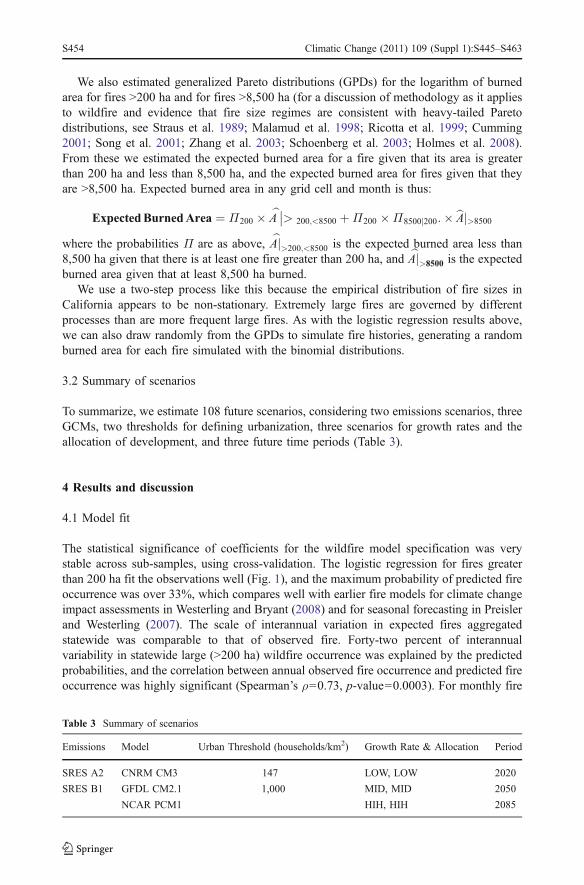
The statistical significance of coefficients for the wildfire model specification was verystable across sub-samples, using cross-validation. The logistic regression for fires greaterthan 200 ha fit the observations well (Fig. 1), and the maximum probability of predicted fireoccurrence was over 33%, which compares well with earlier fire models for climate changeimpact assessments in Westerling and Bryant (2008) and for seasonal forecasting in Preislerand Westerling (2007). The scale of interannual variation in expected fires aggregatedstatewide was comparable to that of observed fire. Forty-two percent of interannualvariability in statewide large (>200 ha) wildfire occurrence was explained by the predictedprobabilities, and the correlation between annual observed fire occurrence and predicted fireoccurrence was highly significant (Spearman’s ρ=0.73, p-value=0.0003). For monthly fire

Table 3 Summary of scenarios

Emissions Model Urban Threshold (households/km2) Growth Rate & Allocation Period

SRES A2 CNRM CM3 147 LOW, LOW 2020

SRES B1 GFDL CM2.1 1,000 MID, MID 2050

NCAR PCM1 HIH, HIH 2085

S454 Climatic Change (2011) 109 (Suppl 1):S445–S463

occurrence aggregated statewide, 58% of month-to-month variability was explained, andthe correlation was also highly significant (Spearman’s ρ=0.84, p-value=2e-16). Theadditional skill at the monthly time scale is due to the model fitting the seasonal cycle in theincidence of fires >200 ha, as well as the interannual variability.

Results for our estimation of the frequency of fires greater than 8,500 ha were alsosignificant, but the skill was lower. This is likely due to both the small number of observedfires of this magnitude, and also it is likely that the size of these fires is highly sensitive tofactors we are not able to consider here, such as the management strategy on individualfires, meteorological conditions on hourly to daily timescales during the fire, andlandsurface characteristics at finer scales than those practical here (~12 km). Twentypercent of interannual variability in statewide very large (>8,500 ha) wildfire occurrencewas explained by the predicted probabilities, and the correlation between annual observedand predicted very large fire occurrence was significant (Spearman’s ρ=0.46, p-value=0.04). Similarly, monthly predicted very large fire occurrence explained 23% of thevariation in observed monthly values, and the correlation was highly significant (Spear-man’s ρ=0.46, p-value<7e-14).

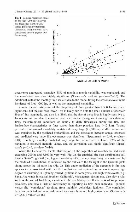
While the Generalized Pareto Distribution fit the logarithm of monthly burned areasexceeding 200 ha and 8,500 ha very well (Fig. 2), the empirical fire size distributions stillhave a “fatter” right tail (i.e., higher probability of extremely large fires) than estimated bythe modeled distributions, as indicated by the values to the far right in the Quantile plotssitting above the 1:1 ratio line (Fig. 2). This under-prediction of the extremes in fire sizeappears to be associated with two factors that are not captured in our modeling—a highdegree of clustering in lightning-caused ignitions in some years, and high wind events (e.g.Santa Ana winds in coastal Southern California). Management factors may also play a role,such as the use of backfires, variation in the availability or effectiveness of suppressionresources, and also a lack of consistency in reporting as fires both individual ignitionsversus fire “complexes” resulting from multiple, coincident ignitions. The correlationbetween predicted and observed burned area was, however, highly significant (Spearman’sρ=0.82, p-value<2e-16).

Fig. 1 Logistic regression modelfit for fires>200 ha: Observedfire frequency (vertical axis)versus predicted probabilities(horizontal axis), binomial 95%confidence interval (upper andlower lines)

Climatic Change (2011) 109 (Suppl 1):S445–S463 S455

Generalized Pareto Distributions can be fit with covariates such as climate and landsurface characteristics, such that the parameters describing the distribution vary over timeand space (see e.g., Holmes et al. 2008). We tested the full suite of predictor variablesdescribed in the preceding sections. While some of them were highly significantstatistically, in practice including covariates had a trivial impact on our ability to predictyear-to-year variations in burned area. Consequently, the results reported here use GPD fitsassuming stationarity (i.e., that the fire size distribution does not change over time). Thus,the interannual variation in our predicted burned area is due entirely to variation inestimated probabilities for burned area to exceed the two specified thresholds (200 ha and8,500 ha).

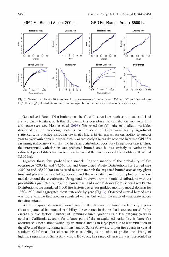
Together these four probabilistic models (logistic models of the probability of fireoccurrence >200 ha and >8,500 ha, and Generalized Pareto Distributions for burned area>200 ha and >8,500 ha) can be used to estimate both the expected burned area at any giventime and place in our modeling domain, and the associated variability implied by the fourmodels around those estimates. Using random draws from binomial distributions with theprobabilities predicted by logistic regressions, and random draws from Generalized ParetoDistributions, we simulated 1,000 fire histories over our gridded monthly model domain for1980–1999, and aggregated them statewide by year (Fig. 3). Observed annual burned areawas more variable than median simulated values, but within the range of variability acrossthe simulations.

While for aggregate annual burned area for the state our combined models only explainabout a quarter of interannual variability, the extremes in the residuals are accounted for byessentially two factors. Clusters of lightning-caused ignitions in a few outlying years innorthern California account for a large part of the unexplained variability in large fireoccurrence. Unexplained variability in burned area is in large part due to a combination ofthe effects of these lightning ignitions, and of Santa Ana-wind driven fire events in coastalsouthern California. Our climate-driven modeling is not able to predict the timing oflightning ignitions or Santa Ana winds. However, this range of variability is represented in

GPD Fit: Burned Area > 200 ha GPD Fit, Burned Area > 8500 ha

Fig. 2 Generalized Pareto Distributions fit to occurrence of burned area >200 ha (left) and burned area>8,500 ha (right). Distributions are fit to the logarithm of burned area and assume stationarity

S456 Climatic Change (2011) 109 (Suppl 1):S445–S463

the probabilities associated with fire occurrence and size in our models, and thussimulations using these probabilities do encompass the variability observed in burned area(Fig. 3).

4.2 Changes in California wildfire

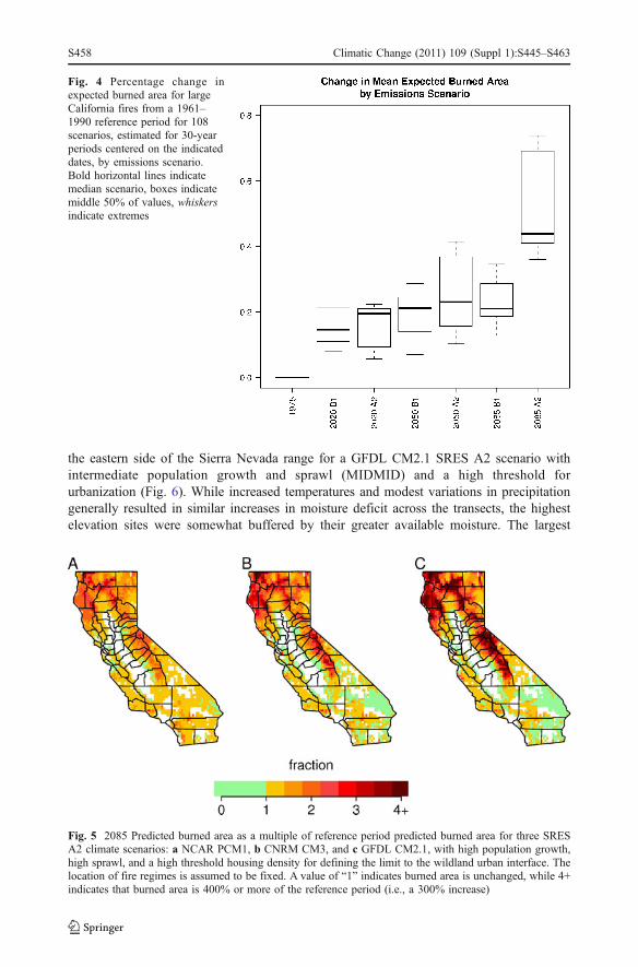
Predicted large fire occurrence and total burned area increase over time for both emissionsscenarios (Fig. 4).2 Initial increases for burned area are relatively modest, with littledifference between emissions scenarios—by 2020 the increases range from 6% to 23%,with median increases between 15% and 19%. By 2050 the spread in modeled outcomeswidens, with predicted increases in burned area ranging from 7% to 41%, and medianincreases between 21% and 23%, but again differences due to emissions scenarios arerelatively small compared to other factors. By 2085, the range of modeled outcomes is verylarge, with total burned area increasing anywhere from 12% to 74%. On average, the largestincreases occur in 2085 for SRES A2 scenarios, with a median statewide increase in burnedarea of 44%, and the biggest increases occurring for the warmer, drier GFDL CM2.1 andCNRM CM3 model runs (range: 38%–74%, median 56%).

The SRES A2 scenarios in 2085 seem to be qualitatively different from either earlierperiods or SRES B1 in 2085 (Fig. 4), implying that the most important policy implicationof this study may be that moving to an emissions pathway more like that in SRES B1 (orlower) could be highly advantageous.

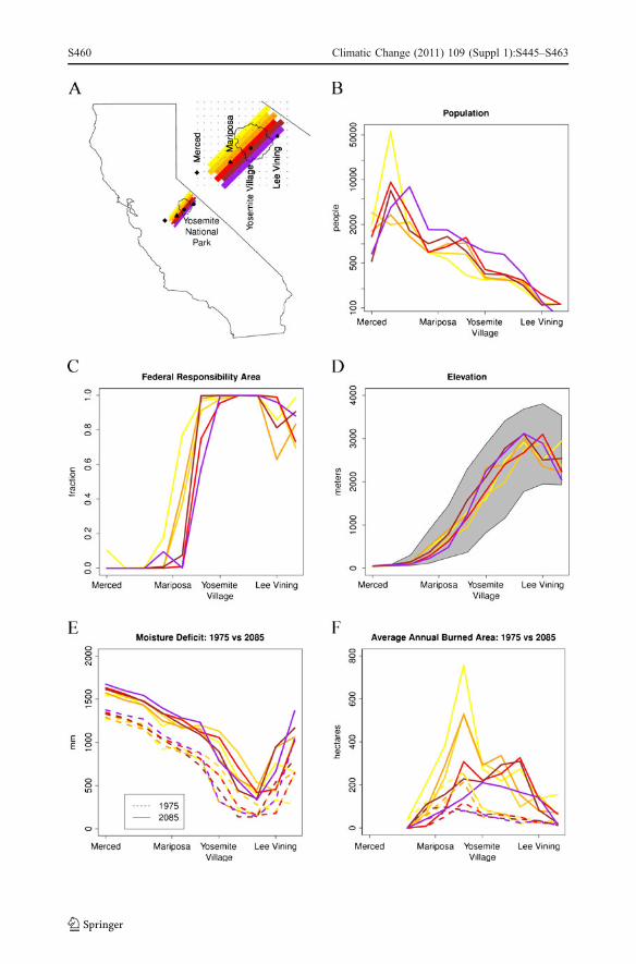
A robust result of this study is that forest burned area increases substantially—exceedingincreases of 100% throughout much of the forested areas of Northern California—across allthree of the GCMs analyzed here for the SRES A2 emissions scenario by 2085 (Fig. 5). Tohighlight the effects of potential increases in forest burned area, we analyzed a set oftransects running from the edge of California’s Central Valley near Merced northwestthrough the Sierra Foothills and Yosemite National Park to Mono Lake and Lee Vining on

2 We show results for expected total area burned only, which are similar to predicted changes in large fireoccurrence.

Fig. 3 Median (horizontal lines),interquartile range (box),extremes within 1.5 x interquar-tile range (whiskers) andextremes outside 1.5 x interquar-tile range are shown for annualburned area aggregated statewidefor 1,000 simulations versus ob-served (red line) burned area forlarge fires in California. Predictedprobabilities of large fires fromlogistic regressions, and General-ized Pareto distributions of firesize, were used to generate 1,000simulations of burned area foreach grid cell and month and thenaggregated by year for the statefor each simulation

Climatic Change (2011) 109 (Suppl 1):S445–S463 S457

the eastern side of the Sierra Nevada range for a GFDL CM2.1 SRES A2 scenario withintermediate population growth and sprawl (MIDMID) and a high threshold forurbanization (Fig. 6). While increased temperatures and modest variations in precipitationgenerally resulted in similar increases in moisture deficit across the transects, the highestelevation sites were somewhat buffered by their greater available moisture. The largest

Fig. 4 Percentage change inexpected burned area for largeCalifornia fires from a 1961–1990 reference period for 108scenarios, estimated for 30-yearperiods centered on the indicateddates, by emissions scenario.Bold horizontal lines indicatemedian scenario, boxes indicatemiddle 50% of values, whiskersindicate extremes

Fig. 5 2085 Predicted burned area as a multiple of reference period predicted burned area for three SRESA2 climate scenarios: a NCAR PCM1, b CNRM CM3, and c GFDL CM2.1, with high population growth,high sprawl, and a high threshold housing density for defining the limit to the wildland urban interface. Thelocation of fire regimes is assumed to be fixed. A value of “1” indicates burned area is unchanged, while 4+indicates that burned area is 400% or more of the reference period (i.e., a 300% increase)

S458 Climatic Change (2011) 109 (Suppl 1):S445–S463

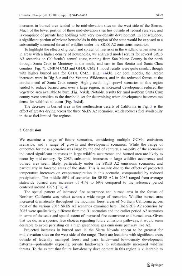
increases in burned area tended to be mid-elevation sites on the west side of the Sierras.Much of the lower portion of these mid-elevation sites lies outside of federal reserves, andis comprised of private land holdings with very low-density development. In consequence,a significant portion of private households in this region of the state would be exposed to asubstantially increased threat of wildfire under the SRES A2 emissions scenarios.

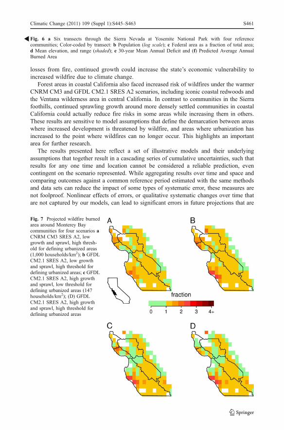
To highlight the effects of growth and sprawl on fire risks in the wildland urban interfacein areas with a higher density of households, we analyzed model results for several SRESA2 scenarios on California’s central coast, running from San Mateo County in the norththrough Santa Cruz to Monterey in the south, and east to San Benito and Santa Claracounties (Fig. 7). CNRM CM3 and GFDL CM2.1 model results were quite similar, thoughwith higher burned area for GFDL CM2.1 (Fig. 7a&b). For both models, the largestincreases were in Big Sur and the Ventana Wilderness, and in the redwood forests at thenorthern end of Santa Cruz county. High-growth, high-sprawl scenarios in this regiontended to reduce burned area over a large region, as increased development reduced thevegetated area available to burn (Fig. 7c&d). Notably, results for rural northern Santa Cruzcounty were sensitive to the threshold set for determining when development becomes toodense for wildfires to occur (Fig. 7c&d).

The decrease in burned area in the southeastern deserts of California in Fig. 5 is theeffect of greater drying across the three SRES A2 scenarios, which reduces fuel availabilityin these fuel-limited fire regimes.

5 Conclusion

We examine a range of future scenarios, considering multiple GCMs, emissionsscenarios, and a range of growth and development scenarios. While the range ofoutcomes for these scenarios was large by the end of century, a majority of the scenariosindicated significant increases in large wildfire occurrence and burned area are likely tooccur by mid-century. By 2085, substantial increases in large wildfire occurrence andburned area seem likely, particularly under the SRES A2 emissions scenarios, andparticularly in forested areas of the state. This is mainly due to the effects of projectedtemperature increases on evapotranspiration in this scenario, compounded by reducedprecipitation. The middle 50% of scenarios for SRES A2 in 2085 ranged from averagestatewide burned area increases of 41% to 69% compared to the reference periodcentered around 1975 (Fig. 4).

The spatial pattern of increased fire occurrence and burned area in the forests ofNorthern California was robust across a wide range of scenarios. Wildfire burned areaincreased dramatically throughout the mountain forest areas of Northern California acrossmost of the various 2085 SRES A2 scenarios examined here. The SRES A2 scenarios by2085 were qualitatively different from the B1 scenarios and the earlier period A2 scenariosin terms of the scale and spatial extent of increased fire occurrence and burned area. Giventhat we do, as a species, face choices regarding future emissions pathways, it would seemdesirable to avoid persisting on a high greenhouse gas emissions pathway like A2.

Projected increases in burned area in the Sierra Nevada appear to be greatest formid-elevation sites on the west side of the range. These are locations with significant areasoutside of federally managed forest and park lands—and low-density developmentpatterns—potentially exposing private landowners to substantially increased wildfirethreats. To the extent that future low-density development in this region is vulnerable to

Climatic Change (2011) 109 (Suppl 1):S445–S463 S459

S460 Climatic Change (2011) 109 (Suppl 1):S445–S463

losses from fire, continued growth could increase the state’s economic vulnerability toincreased wildfire due to climate change.

Forest areas in coastal California also faced increased risk of wildfires under the warmerCNRM CM3 and GFDL CM2.1 SRES A2 scenarios, including iconic coastal redwoods andthe Ventana wilderness area in central California. In contrast to communities in the Sierrafoothills, continued sprawling growth around more densely settled communities in coastalCalifornia could actually reduce fire risks in some areas while increasing them in others.These results are sensitive to model assumptions that define the demarcation between areaswhere increased development is threatened by wildfire, and areas where urbanization hasincreased to the point where wildfires can no longer occur. This highlights an importantarea for further research.

The results presented here reflect a set of illustrative models and their underlyingassumptions that together result in a cascading series of cumulative uncertainties, such thatresults for any one time and location cannot be considered a reliable prediction, evencontingent on the scenario represented. While aggregating results over time and space andcomparing outcomes against a common reference period estimated with the same methodsand data sets can reduce the impact of some types of systematic error, these measures arenot foolproof. Nonlinear effects of errors, or qualitative systematic changes over time thatare not captured by our models, can lead to significant errors in future projections that are

Fig. 7 Projected wildfire burnedarea around Monterey Baycommunities for four scenarios aCNRM CM3 SRES A2, lowgrowth and sprawl, high thresh-old for defining urbanized areas(1,000 households/km2); b GFDLCM2.1 SRES A2, low growthand sprawl, high threshold fordefining urbanized areas; c GFDLCM2.1 SRES A2, high growthand sprawl, low threshold fordefining urbanized areas (147households/km2); (D) GFDLCM2.1 SRES A2, high growthand sprawl, high threshold fordefining urbanized areas

Fig. 6 a Six transects through the Sierra Nevada at Yosemite National Park with four referencecommunities; Color-coded by transect: b Population (log scale); c Federal area as a fraction of total area;d Mean elevation, and range (shaded); e 30-year Mean Annual Deficit and (f) Predicted Average AnnualBurned Area

R

Climatic Change (2011) 109 (Suppl 1):S445–S463 S461

not encompassed by the range of uncertainty represented in our results. That is, the resultsare conditional not only on the storylines of the SRES A2 and B1 scenarios and choice ofglobal climate models, but also on the specifications of the statistical models of fire activitythat we have estimated from historic data. To the extent that these data reflect processes thatwill no longer operate in the future because of qualitative changes to the systems we aremodeling, our results will be in error.

Our results project the current managed fire regimes of California onto future scenariosfor climate and for population and development footprint. We do not consider hypotheticaleffects of future changes in management strategies, technology, or resources that might beadopted with the intent of mitigating or adapting to the effects of climate and developmenton wildfire. Our models’ implicit assumptions that such management effects are fixed mayprove untenable under some future scenarios. Explicitly including management factors thatcan vary over the long term might significantly affect the outcomes modeled here in asystematic fashion. Such an exercise is left to a future study.

While we do not model metrics of fire severity (e.g., percent of vegetation consumed,ecological impact of burning) here, we expect that fire severity may be correlated withincreases in fire occurrence and spatial extent in some ecosystems, particularly in somemountain forest areas of the state. It seems likely that outcomes such as those describedhere would have important implications for ecosystem services such as carbon sequestrationin California forests, air pollution and public health, forest products and recreationindustries, and the quality and timing of runoff from precipitation and snowmelt. All ofthese merit intensive further study.

References

Balling RC, Meyer GA, Wells SG (1992) Relation of surface climate and burned area in yellowstone nationalpark. Agric For Meteorol 60:285–293

Brillinger DR, Preisler HK, Benoit JW (2003) Risk assessment: a forest fire example. In Science andStatistics, Institute of Mathematical Statistics Lecture Notes. Monograph Series

Cayan D, Tyree M et al (2009) Climate Change scenarios and sea level rise estimates for the California 2008Climate Change Scenarios Assessment, Public Interest Energy Research, California Energy Commision,Sacramento, CA

Cumming SG (2001) A parametric model of the fire-size distribution. Can J For Res 31:1297–1303Gesch DB, Larson KS (1996) Techniques for development of global 1-kilometer digital elevation models. In

Pecora Thirteen, Human Interactions with the Environment—Perspectives from Space. Sioux Falls,South Dakota, August 20–22, 1996

Hamlet AF, Lettenmaier DP (2005) Production of temporally consistent gridded precipitation andtemperature fields for the continental U.S. J Hydrometeorol 6(3):330–336

Hansen MC, DeFries RS, Townshend JRG, Sohlberg R (2000) Global land cover classification at 1 kmspatial resolution using a classification tree approach. Int J Remote Sens 21:1331–1364

Heyerdahl EK, Brubaker LB, Agee JK (2001) Factors controlling spatial variation in historical fire regimes: amultiscale example from the interior West, USA. Ecology 82(3):660–678

Hidalgo HG, Dettinger MD, Cayan DR (2008) Downscaling with constructed analogues: Daily precipitationand temperature fields over the United States. CEC Report CEC-500-2007-123. January 2008

Holmes TP, Hugget RJ, Westerling AL (2008) Statistical analysis of large wildfires. Chapter 4 of economicsof forest disturbance: Wildfires, storms, and pests, Series: Forestry Sciences, Vol. 79. In Holmes TP,Prestemon JP, Abt KL (Eds), XIV, p 422. Springer. ISBN: 978-1-4020-4369-7

Kipfmueller KF, Swetnam TW (2000) Fire-climate interactions in the Selway-Bitterroot wilderness area.USDA Forest Service Proceedings RMRS-P-15-vol-5

Le Quéré C, Raupach MR, Canadell JG, Marland G (2009) Trends in the sources and sinks of carbondioxide. Nat Geosci 2:831–836

S462 Climatic Change (2011) 109 (Suppl 1):S445–S463

Liang X, Lettenmaier DP, Wood EF, Burges SJ (1994) A simple hydrologically based model of land surfacewater and energy fluxes for general circulation models. J Geophys Res 99(D7):14,415–14,428

Malamud BD, Morein G, Turcotte DL (1998) Forest fires: an example of self-organized critical behavior.Science 281:1840–1842

Maurer EP, Hidalgo HG (2008) Utility of daily vs. monthly large-scale climate data: an intercomparison oftwo statistical downscaling methods. Hydrology and Earth System Science 12:551–563

Maurer EP, Wood AW, Adam JC, Lettenmaier DP, Nijssen B (2002) A long-term hydrologically-based dataset of land surface fluxes and states for the conterminous United States. J Climate 15:3237–3251

Mitchell KE et al (2004) The multi-institution North American Land Data Assimilation System (NLDAS):Utilizing multiple GCIP products and partners in a continental distributed hydrological modeling system.J Geophys Res 109:D07S90. doi:10.1029/2003JD003823

Monteith JL (1965) Evaporation and the environment. Symp Soc Expl Biol 19:205–234Penman HL (1948) Natural evaporation from open-water, bare soil, and grass. Proc R Soc Lond A193

(1032):120–146Preisler HK, Westerling AL (2007) Statistical model for forecasting monthly large wildfire events in the

Western United States. J Appl Meteorol Climatol 46(7):1020–1030. doi:10.1175/JAM2513.1Preisler HK, Westerling AL, Gebert KM, Munoz-Arriola F, Holmes T (2011) Spatially explicit forecasts of

large wildland fire probability and suppression costs for California. International Journal of WildlandFire 20:508–517

Preisler HK, Brillinger DR, Burgan RE, Benoit JW (2004) Probability based models for estimating wildfirerisk. Int J Wildland Fire 13:133–142

Ricotta C, Avena G, Marchetti M (1999) The flaming sandpile: self-organized criticality and wildfires. EcolModel 119:73–77

Schlobohm P, Brain J (2002) Gaining an understanding of the national fire danger rating system. NationalWildfire Coordinating Group Publication: NFES # 2665. www.nwcg.gov

Schoenberg FP, Peng R, Woods J (2003) On the distribution of wildfire sizes. Environmetrics 14:583–592Song W, Weicheng F, Binghong W, Jianjun Z (2001) Self-organized criticality of forest fire in China. Ecol

Model 145:61–68Stephenson NL (1998) Actual evapotranspiration and deficit: Biologically meaningful correlates of

vegetation distribution across spatial scales. J Biogeog 25:855–870Strauss D, Bednar L, Mees R (1989) Do one percent of the forest fires cause ninety-nine percent of the

damage? Forest Sci 35:319–328Swetnam TW, Betancourt JL (1998) Mesoscale disturbance and ecological response to decadal climatic

variability in the American Southwest. J Clim 11:3128–3147Theobald D (2005) Landscape patterns of exurban growth in the USA from 1980 to 2020. Ecol Soc 10(1):32U.S. EPA (2008) Preliminary steps towards integrating climate and land use (ICLUS): The Development of

Land-Use Scenarios Consistent with Climate Change Emissions Storylines (External Review Draft). U.S. Environmental Protection Agency, Washington, D.C. EPA/600/R-08/076A

Veblen TT, Kitzberger T, Donnegan J (2000) Climatic and human influences on fire regimes in ponderosapine forests in the Colorado Front Range. Ecol Appl 10:1178–1195

Verdin KL, Greenlee SK (1996) Development of continental scale digital elevation models and extraction ofhydrographic features. In: Proceedings, Third International Conference/Workshop on Integrating GISand Environmental Modeling, Santa Fe, New Mexico, January 21–26, 1996. National Center forGeographic Information and Analysis, Santa Barbara, California

Westerling AL (2009) “Wildfires.” Chapter 8 in Climate Change Science and Policy. Schneider, Mastrandrea,Rosencranz and Kuntz-Duriseti (Eds), Island Press”Washington DC, USA

Westerling AL, Bryant BP (2008) Climate change and wildfire in California. Clim Chang 87:s231–249.doi:10.1007/s10584-007-9363-z

Westerling AL, Gershunov A, Cayan DR, Barnett TP (2002) Long lead statistical forecasts of Western U.S.Wildfire area burned. Int J Wildland Fire 11(3,4):257–266. doi:10.1071/WF02009

Westerling AL, Brown TJ, Gershunov A, Cayan DR, Dettinger MD (2003) Climate and wildfire in theWestern United States. Bull Am Meteorol Soc 84(5):595–604

Westerling AL, Hidalgo HG, Cayan DR, Swetnam TW (2006) Warming and earlier spring increases WesternU.S. forest wildfire activity. Science 313:940–943. doi:10.1126/science.1128834, Online supplement

Zhang Y-H, Wooster MJ, Tutubalina O, Perry GLW (2003) Monthly burned area and forest fire carbonemission estimates for the Russian Federation from SPOT VGT. Remote Sens Environ 87:1–15

Climatic Change (2011) 109 (Suppl 1):S445–S463 S463