Climate Change, Contagion and Conservation: Valuing Services and Evaluating Policies in Brazil via Applied CGE

Subhrendu K. Pattanayak, Martin T. Ross, Brooks M. Depro,

Simone C. Bauch, Christopher Timmins, Kelly J. Wendland, and Keith Alger1

Abstract

Ecosystems are the planet’s life support system. Why then is ecosystem degradation excessive or so rapid? Unfortunately, the answer to this question is currently obscured by some conceptual confusion and lack of reliable data and methods for ecosystem valuation. We contend that provision of ecosystem services is sub-optimal because ecosystem services are public goods, ecosystem management involves externalities and ecosystems are often the only capital of the poor who have no money or political voice. These features also complicate efforts to develop credible estimates of ecosystem values because of limitations of appropriately scaled the data (often from other disciplines) and internally consistent methods. Consequently, policy makers lack good information to design and implement salient policies. We develop a case study for Brazil to illustrate how econometric estimation can be combined with computable general equilibrium (CGE) modeling to estimate ecosystem values associated with climate change and forest conservation. Econometric analysis of Brazilian regional data shows that climate change will increase morbidity (e.g., almost a 0.5% impact on labor endowment) and forest conservation can mediate climate impacts (by almost 20%). CGE simulations using econometric parameters suggest substantial economic impacts originating in land and labor markets. Thus, there is potential for significant ecosystem services (increased human welfare) via the disease regulation pathway. Moreover, a preliminary biodiversity assessment suggests that for many species, which would otherwise lose 50% of their range, ecosystem protection represents insurance against future extinction risk.

Prepared for presentation at the Association of Environmental and Resource Economics annual workshop on Valuation and Incentives for Ecosystem Services

in Mystic, Connecticut, June, 2007.

1 Address correspondence to Subhrendu K. Pattanayak, Fellow and Senior Economist, Public Health and

Environment Division, RTI International; Research Associate Professor, North Carolina State University, and Visiting Scholar, University of California at Berkeley (subhrendu@rti.org). Ross (mross@rti.org) and Depro are in the Technology, Energy and Environmental Economics program at RTI International. Bauch is with Imazon and the Department of Forestry in NC State University. Timmins is at the Economics Department at Duke University (timmins@econ.duke.edu). Wendland and Alger (k.alger@conservation.org) are in the Center for Applied Biodiversity Sciences at Conservation International. We are grateful to Erin Sills and Imazon staff for help with different aspects of the data collection and to Miroslav Honzak for the biodiversity assessment. We acknowledge comments from workshop participants at workshops at Duke University’s Nicholas School, the U.S. EPA, and the University of Wisconsin, Madison.

1

I. INTRODUCTION The Millennium Ecosystem Assessment (MEA) – a global multi-institutional, multi-year

initiative – finds that humans have altered ecosystems more rapidly in the past 50 years than at any other time in human history (MEA 2005). The MEA also concludes that the drivers of change show no evidence of decline and in many cases will increase in intensity. These changes come at the expense of losses in biodiversity and ecosystem functions – severely endangering the flow of socially valuable goods and services, particularly for the poor in the developing world. Given the correlations between ecosystem services and human well-being, we might wonder why ecosystem degradation is excessive or rapid. Unfortunately, the answer to this question is currently obscured by some conceptual confusion and lack of reliable data and methods for ecosystem valuation. Economists readily relate to the notion of suboptimal provision of ecosystem services because ecosystem services are public goods, ecosystem management involves externalities and ecosystems are often the only capital of the poor who have no money or political voice. These features also complicate efforts to develop credible estimates of ecosystem values because of limitations of appropriately scaled the data (often from other disciplines) and internally consistent methods. Consequently, policy makers lack good information to design and implement salient policies. In this paper, we present a broad review of ecosystem valuation, summarizing its role in the design and implementation of institutions to deliver ecosystem services. We illustrate how robust and flexible econometric estimation can be combined with computable general equilibrium (CGE) modeling to estimate ecosystem values.

Our case study focuses on ecosystem services in Brazil related to the control of infectious disease, and is developed against a backdrop of climate change and biodiversity conservation, two of the most profound ecosystem changes facing the world. Specifically, we consider a moderate IPCC warming scenario that is expected to raise temperature by an average of 2˚C and cause in fluctuations in rainfall of ± 15% in the neo Tropics (Hulme and Sheard, 1999). We overlay on this a very ambitious policy of the Brazilian government to expand its system of National Forests (FLONAS) by 50 million hectares (Verissimo et al., 2002), a scale that is unprecedented in the tropics and matched in ambition only by the U.S. park system. Consequently, we develop and use a CGE model, focusing on adjustments to land and labor markets, to look at these profound changes to the environment.

An extensive epidemiology and environmental sciences literature documents the multiple links between climate change, deforestation and illnesses (e.g., Patz et al., 1996; Yasuoka and Levins, 2005). Unfortunately, this literature does not provide parameters to assess economy-wide health implications. Thus, we build a data set of 484 Brazilian micro-regions in the 1990 – 2000 vintage by integrating records from various Brazilian public agencies and line ministries on (a) morbidity (b) long run temperature and rainfall from weather station records, (c) housing, water and sanitation facilities, population, education levels, income, medical care, and infrastructure, (d) forest cover, landuse and protected areas. Robust estimation shows that hotter and wetter climate is associated with higher rates of dengue, malaria, cardio vascular and respiratory diseases. Quantile regressions also show that the establishment of protected areas, particular in the Amazon where much of the deforestation is occurring, is correlated with lower malaria.

Estimated regression parameters are used to develop expected changes in the disease profile associated with the climate change and protected areas scenarios. Following Jorgenson et al., we conceptualize health impacts in the CGE via labor market. The econometric estimates of health effects are translated into reductions in labor endowment by converting additional cases of morbidity into ‘healthy’ years lost due to disability and then representing as a percentage change in labor endowment. We predict an annual reduction in the labor endowment of 0.47% because of climate change and of 0.39%, if climate change is mediated by FLONAS conservation.

The dynamic CGE model developed for this exercise covers all parts of the economy, allows us to link sectors, industries and countries. The model has 3 regions (Brazil, rest of South

2

America, rest of the world), 12 agricultural sectors and forestry that are land users (where land is divided into 18 agro-ecological zones) and 12 other sectors. The “no action baseline” is essentially a 0.47% reduction in labor and deforestation of 3 million hectares. This is contrasted with a “FLONAS scenario” that involves a morbidity impact of 0.39% and sustainable timber production (which increases managed lands by approximately 10 times). We find that the FLONAS scenario results in higher GDP, lower wage rates, higher investments, lower household consumption, higher imports and exports, decline in agriculture (less land available) and increase in production of other industries. Thus, the $120 million (prevented GDP decline) represents a first-order approximation of the ecosystem services from conservation via the pathway of regulating infectious diseases.

II. ECOSYSTEM SERVICES The MEA adopts the concept of ecosystem as its organizing framework, where

ecosystem is defined as “a dynamic complex of plant, animal and micro-organism communities and their nonliving environment interacting as a functional unit”. This ‘ecosystem approach’ is meant to facilitate conservation, sustainable use, and fair and equitable sharing of resources (MEA 2005a). The MEA (2005a) defines four types of ecosystem services: provisioning, regulating, supporting, and cultural. ‘Provisioning’ refers to those services which are vital for supplying the basic materials of life, such as food, fiber, fresh water, and genetic materials. ‘Regulating’ refers to those services that support life, such as the mitigation of floods and droughts, the purification of air and water, climate regulation, and disease regulation. ‘Supporting’ refers to those services that directly support life, such as primary production of biomass, nutrient cycling, and soil formation. ‘Cultural’ refers to any services that enrich human life, including the aesthetic values, spiritual components, and social relations that ecosystems provide.

Here we briefly review the linkages between human health and ecosystem intactness and functioning, a key ‘regulating service’, by drawing extensively from Corvalan, Hayles, McMichael et al. (2005). As illustrated in figure SDM1 in their report, escalating human pressure on the global environment has impaired ecosystems in various ways, including but not limited to: biodiversity loss, coastal reef damage, urbanization, climate change, stratospheric ozone depletion, deforestation and land cover change, wetland loss and damage, and freshwater depletion and contamination. These profound environmental changes can cause health impacts through at least three pathways: direct, ecosystem-mediated, and indirect-displaced-deferred. The direct health impacts typically result from ecosystem changes such as floods, heatwaves, droughts, landslides, exposure to pollution and ultraviolet radiation. Ecosystem-mediated health impacts are associated with altered infectious disease risk, reduced food yields (malnutrition, stunting), depleted natural medicines, mental health, and aesthetic and cultural impoverishment. The indirect-displaced impacts relate to the varied health consequences of livelihood loss, population displacement (e.g., dwelling in slums), conflict, and inappropriate adaptation and mitigation.

As Corvalan et al. (2005) clarify, the “causal link from ecosystem change to human health are complex because often they are indirect, displaced in space and time, and dependent on a number of modifying forces.” Thus, we focus this review on the objectives of this paper and present a further synthesis of the ‘ecosystem-mediated’ impacts – particularly the regulation of infectious diseases (see Patz et al. [2005] for further details). Infectious agents such as viruses, bacteria and microbes are constrained by the geographical and seasonal dimensions of ecosystems as well as ecological relationships in nature. The magnitude and direction of infectious diseases attributable to ecosystem changes are specific to ecosystems and types of land uses, to disease-specific transmission dynamics, and to the susceptibility of human populations. The reasons for the emergence or re-emergence of some diseases are unknown, but the main biological

3

mechanisms that have altered the incidence of many infectious diseases are clear. These include: (a) altered habitat features leading to changes in the number of vector breeding sites or reservoir host distribution; (b) niche invasions of new species or interspecies host transfers; (c) changes in biodiversity, including loss of predator species and changes in host population density; (d) human-induced genetic changes of disease vectors or pathogens (such as mosquito resistance to pesticides or emergence of antibiotic-resistant bacteria); and (e) environmental contamination by infectious disease agents. Numerous disease/ecosystem relationships illustrate these biological mechanisms. As Patz et al. point out, the infectious diseases of major public health importance that require special attention due to ecosystem changes, but also have the greatest potential for risk reduction by planned interventions include: malaria, across most ecological systems; dengue fever in tropical urban centres; schistosomiasis and filariasis in cultivated and inland water systems in the tropics; leishmaniasis in forest and dryland systems; cholera in coastal and urban systems; cryptosporidiosis in agricultural systems; Japanese encephalitis in agricultural systems; and West Nile virus and Lyme disease in urban/suburban systems of Europe and North America. It is impossible to review in any detail the entire suite of human influenced ecosystem changes and their human health consequences. Therefore, we use examples of climate change and deforestation to illustrate the basic point.

Climate Change and diseases Ecosystems can affect climate in numerous ways: in terms of warming, as sources of

greenhouse gases; and in terms of cooling, as sinks of greenhouse gases. Climatic heating and cooling mechanisms also are influenced by albedo, or ecosystem reflectivity to solar radiation, e.g. forests absorb heat energy, and thus have lower albedo than snow, which reflects solar radiation. Natural aerosols (e.g. dust) also reflect solar radiation. Ecosystems affect climate through patterns of evapotranspiration and cloud formation, water redistribution/recycling, and regional rainfall. Ecosystems affect air quality through interactions with atmospheric cleansing processes (e.g. as sinks for air pollutants and sources of pollution such as particulates from biomass combustion); and through nutrient redistribution (e.g. fertilizing effects of nitrogen deposition, carbon dioxide and dust). Anthropogenic stressors such as deforestation, desertification and greenhouse gas emissions can profoundly alter the role of natural ecosystems in regulating climate.

The resulting climate change in turn can impact health in the following ways. First, climate change, excessive temperatures, and heat waves can alter arterial pressure, blood viscosity and heart rate causing cardiovascular and cereberovascular diseases among elderly. Second, thermal stress and temperature related air pollution (thermal inversion), pollen counts, mold growth and pollution precursor (NO based ozone) can cause a variety of respiratory diseases including asthma, bronchitis, pneumonia, cough & cold. Third, increasing temperatures, humidity and rainfall can affect proliferation, density, behavior, variety, viability, and maturation of mosquitoes that carry malaria and dengue parasites. Fourth, climate change can indirectly impact nutrition through its impact on agriculture yield (see McMichael et al. [1996], Martens [1998], Patz et al. [1996] for further details).

Deforestation and Malaria While a number of anthropogenic land use changes have the potential to affect the

emergence, reemergence, and spread of infectious diseases (Patz et al., 2004, Lindsay & Birley, 2004), the relationship between deforestation and malaria is particularly important (Pattanayak et al., 2006; Pattanayak and Yasuoka, forthcoming). As Patz et al. (2004) note, deforestation has accompanied increases in malaria in Africa, Asia, and Latin America. Deforestation is often a precursor to other important land use changes, such as agricultural expansion and intensification. Deforestation has also attracted substantial policy attention and innovation, with potential cross-effects on malaria. Thus, while we recognize the importance of other processes (e.g.,

4

urbanization) in the evolution of malaria, this paper focuses primarily on deforestation. In particular, a review of the literature (Wilson, 2001; Patz et al., 2000; Walsh et al., 1993, Patz et al., 2004, Molyneux, 2003) reveals five potential pathways through which forest management and deforestation can affect malaria infection and disease transmission. 1. Deforestation changes the ecology of a disease vector and its options for hosts. Whereas the

forest floor in primary growth tends to be heavily shaded and littered with a thick layer of organic matter that absorbs water and renders it quite acidic, cleared lands are generally more sunlit and on flat terrain, are prone to the formation of puddles with more neutral pH which can favor specific anopheline larvae development (Patz et al., 2000).

2. Deforestation can affect climate at local, regional, and even global scales (through impacts on the global carbon cycle). Where the scale of deforestation is large, e.g. the Amazon basin, the effects on temperature and moisture and therefore on vector habitats could potentially be quite significant (Wilson, 2001). Higher temperatures can increase the rate at which mosquitoes develop into adults, the frequency of their blood feeding, the rate at which parasites are acquired, and the incubation of the parasite within mosquitoes (Walsh et al., 1993). For example, deforestation and its related activities have produced new habitats for Anopheles darlingi mosquitoes and have been correlated with malaria epidemics in South America (Walsh et al., 1993). The different species complexes in SE Asia (A. dirus, A. minimus, A balabacensis) have been affected in different ways by forest clearance with different impacts on malaria incidence (Walsh et al., 1993).

3. Deforestation is often just the first step in a chain of land use changes. These changes may include agriculture and livestock, plantations, human settlement, increased use of regenerating forests, road construction, and water control systems (dams, canals, irrigation systems, reservoirs). Networks of irrigation ditches, canals and impoundments, as well as puddles from road construction, can improve vector habitats. Livestock can change vectorial capacity. Use of insecticide in follow-up agriculture can increase vector resistance (Wilson, 2001).

4. Deforestation is accompanied by migration and other behavioral changes that may enhance the spread of malaria. In the case of gold mines in the Brazilian Amazon, migrants typically have little previous exposure and therefore lower immunity (Castilla and Sawyer, 1993). Moreover, migrants introduce the additional complication associated with administering health services to transient populations—inadequate medical follow up and possible side effects. Although incomplete treatment can relieve fever, the underlying malarial infection persists as the migrant moves and potentially transmits the disease to other locations, often on the deforestation frontier.

Externalities, Public Goods and Non-market Valuation If humans benefit from ecosystem services such as disease regulation, then why are we

experiencing such rapid and wide scale ecosystem degradation such as deforestation and climate change? One view is that the value of ecosystems and the services they provide are over-stated and society degrades the natural ecosystem because they do not provide direct, tangible and near-term benefits, compared to alternative uses of the ecosystem (e.g., logging, cattle, soybean farming). In contrast, we believe that while some of the ecosystem services are familiar (e.g., value of medicinal plants), in general, ecosystem services are insufficiently understood and undervalued – leading to the mismanagement of natural ecosystems.

To understand why ecosystem services are under appreciated and under provided, consider some general insights from public economics concerning ‘externalities’ and ‘public goods’ – two concepts most readily associated with ‘ecosystem services’. First, data on the spatial and temporal impacts of services is often insufficient and unavailable – since services are diffused across space (upstream conservation and downstream benefits) and time (preservation in the past provides services in the future, possibly for another generation), a simple point estimate presents

5

an inadequate picture. Second, the benefits of ecosystem services and the costs of protecting them are often spread across heterogeneous agents. For example, there are several global and regional benefits to protecting services (e.g., carbon sequestration or water purification); however the costs of protecting these systems often accrue locally. Both points above suggest the prevalence of externalities (choices made without regard to broader social consequences) that lower incentives for any one individual to protect these resources. Third, for the reasons suggested above, conventional markets will not reflect the full social costs and benefits of ecosystem services (Panayotou 1992) and emerging markets for ecosystem services (e.g., carbon trading) remain incomplete and thin. Finally, like all public goods, it is difficult to exclude any individual from using these services and several individuals can use the services simultaneously without diminishing the value of the other person. Collectively, these features suggest the presence of major information asymmetries and formidable and prohibitive transaction costs related to learning about and providing ecosystem services. Consequently, we can expect good quality non-market valuation studies to serve a very important purpose.

The onus rests on well-informed governments and civil society to provide the optimal level of ecosystem services because the inherent features of ecosystem services diminish incentives for conservation. The information gap relates to the values of these services – at least some rough and ready estimates of their contribution to human well-being. Armed with information on the value of ecosystem services, policymakers can design and use different types of incentives to change individual behaviors from ecosystem destruction to ecosystem protection. Different conservation tools that have been “in vogue” at different time periods to support biodiversity protection and more recently, protection of ecosystem services (see Polasky et al. 2005 for a more complete review of these policy tools). Below we review how the design and implementation of these tools can draw on valuation information.

The ‘ecosystem approach’ adopted by the MA (2005b) fits optimally into the idea of measuring economic value since the premise of a ‘service’ implies that the outcomes of ecosystem processes are valued by people. Although valuation alone is neither necessary nor sufficient for conservation to work (Heal et al., 2004), economic valuation can provide important inputs into the policy process (Pagiola et al. 2004; Polasky et al. 2005); it can be used to: (1) estimate the relative importance of various ecosystems; (2) justify or evaluate particular conservation decisions in particular places; (3) identify how the benefits of a particular conservation decision are distributed; and (4) identify potential sources of sustainable financing.

The first use of valuation listed requires estimating the total economic value (TEV) – the sum of all the use and non-use values – of an ecosystem. Practical applications of the TEV concept include the development of quality-adjusted-life and green National Accounts, and estimation of compensation in natural resource damage litigation. A more practical application of valuation in the conservation arena is the second reason listed above: to evaluate different forms of management. This can be useful for illuminating tradeoffs among different types of land use options, and tradeoffs between biodiversity conservation and other socially desirable outcomes (e.g., livelihoods). Valuation can also be used to assess the changes in ecosystem services that result from different conservation interventions (e.g., protected areas, national forests) in a certain context to evaluate if the benefits of the particular policy exceed the costs.

The third purpose that valuation is used for is to help understand how the benefits of a particular conservation decision are distributed. Many groups of people benefit from the conversion of natural ecosystems to human-dominated ecosystems and from the exploitation of biodiversity. These gains, however, come at the expense of costs on biodiversity and ecosystem services and the people that rely on these services, such as the poor or indigenous populations (MEA 2005a). The gainers and losers are often not the same. By understanding who “benefits” and who “loses” from conservation on the ground, we can design appropriate conservation incentives that target different stakeholders. If the benefits that accrue to local people from

6

conservation are not sufficient (or in excess of opportunity costs) to change behaviors, the valuation process can help determine direct compensation packages.

A final use of valuation is to help identify potential sources of financing. By measuring the amount of benefits different stakeholders receive (see previous point), valuation can help in the design of incentives for conservation and capture of some of the environmental benefits for conservation financing purposes. This could include setting the appropriate level and type of payments for environmental services (e.g., carbon prices, user fees for water). In addition, understanding the economic worth of benefits provided by ecosystems can provide leverage for more support of global financing mechanisms such as the Global Environmental Facility.

A Framework for Ecosystem Valuation Economic valuation methods typically involve the quantitative estimation of the worth of

a non-market good (e.g., ecosystem service) in terms of a common metric, usually a monetary metric. While money is often a convenient common metric, it is not the only metric; for example, habitat equivalency analysis is another way to compare. At its root, the ‘nonmarket valuation methods’ must link ecosystem process to a related market commodity because most ecosystem services are not traded in conventional markets. Establishing this link allows the economist’s definition of demand to be applied (Freeman 1996), even if the ecosystem services are indirect, subtle, and or latent (Pattanayak and Butry 2005). For example, in many ecosystems pollination services are provided to surrounding agricultural fields. To be able to measure the value of this service, a link must be established between the pollinators and the marketable agricultural crop produced from these services. The most common non-market valuation methods (and the associated markets) used to measure the worth of ecosystem services are hedonic pricing (property and labor market), travel cost (time and recreation goods), productivity analysis (commodities – e.g., timber, crops), and contingent valuation (stated preferences). MEA 2005b presents overviews of the methods and when they should be used).

Irrespective of the method applied, a three-stage analytical framework can be used to understand how ecosystem functions and processes can be linked directly or indirectly to the well-being of people (see Pattanayak [2004] for more detail). The first stage of analysis measures how ecosystem flows (e.g., quantity or rate of stream flow, erosion, or sediment) change as a result of some type of public policy or private action that alters land uses.

The second stage of this framework measures how changes in ecosystem flows change the socioeconomic productivity of an individual. In this stage, an explicit connection must be made between the change in the provision of an ecosystem service and human well-being. In the final stage of the framework, the productivity changes experienced are expressed in monetary terms. When the changes in productivity are directly related to market commodities, then the monetary prices will just be those of the market goods (e.g., coffee, electricity costs, water tariffs). For other cases, the changes in productivity will not be market goods but will be closely related to the production of such goods (e.g., time expended on water collection, lost labor from disease incidence) and the prices associated with these activities (e.g., time, labor) can be used to develop a ‘monetized’ measure of ecosystem service (Pattanayak 2004).

Although non-market valuation methods such hedonic pricing, travel cost, productivity analysis, and contingent valuation are well-established in the environmental economics literature, they are limited in their capacity to measure the value of ecosystem services. This is because ecosystem services are diffused across space and time. Thus, partial equilibrium methods and concepts cannot capture values of ‘off-site’ and future beneficiaries. As Carbone and Smith (2007) contend, computable general equilibrium (CGE) models may be better suited to capture varying impacts over time, and/or wide reaching multi-sectoral consequences of wide-ranging ecosystem changes such as climate variability, rapid biodiversity loss, and deforestation. The results of CGE simulations to evaluate policies, including those that will deliver ecosystem services, are often reported in terms of net gains to the economy. Measurement in terms of its

7

impact on the overall economy seems to be moving us closer in spirit the idea of using an inclusive measure of wealth as an appropriate indicator of value (Dasgupta, 2001). We investigate this strategy in this paper.

III. APPLIED CGE FOR EVALUATION AND VALUATION In contrast to other evaluation frameworks, CGE models can evaluate policy impacts in a

theoretically consistent fashion for policies (a) without historical precedents, (b) with potentially varying impacts over time, and/or (c) wide reaching multi-sectoral consequences. This makes it possible for them to analyze impacts of wide-ranging ecosystem changes attributed to climate variability, rapid biodiversity loss, and deforestation (Carbone and Smith, 2007). Notwithstanding their promise, high quality applications of CGE models to land use change and natural resource management has been scarce (Ross et al., forthcoming). Cattaneo’s work (2001, 2005) represents a well-known peer reviewed CGE model used to examine the causes of deforestation in Brazil. Similarly, Gollin and Zimmerman (2006) and Chakraborty et al. (2007) are initial attempts to examine the general equilibrium consequences of malaria risks. Rarely, however, have such attempts examined the joint implications of biodiversity loss, land use change, and infectious diseases, or reported on non-economic outputs.

Figure 1. Circular Economic Flows in a CGE Model of Brazil

Households

Firms

Households supply labor, capital, and

natural resources

Households receive factor income

Firms produce goods & services

Firms buy goods & services

Households buy goods & services

Imports Exports Capital flows

among regions

Trade & capital flows

Trade & capital flows

Government Taxes Taxes

Factors of Production

(labor, capital, and resources - land)

Goods & Services

Rest of South America

Other Countries

of the World

Firms buy labor, capital, and

natural resources

As described in Ross et al. (forthcoming) in detail, designing a CGE modeling framework begins with a set of equations based on economic theory that describe interactions among businesses, households, governments, and regions of a nation and/or world. Within their structure, CGE models capture all flows of goods and factors of production (labor, capital, and natural resources) in the economy – see Figure 1. The ‘general equilibrium’ nature of these models implies that all sectors in the economy must be in balance and all economic flows must be accounted for within the model. Households own factors of production and sell them to firms, which generates incomes for households. Firms produce output by combining productive factors with intermediate inputs of goods and services from other industries. The output of each industry is purchased by other industries or households using the income received from sales of factors.

8

Goods and services can also be exported, and imported goods can be purchased from other countries. Capital moves among regions as they run trade deficits or surpluses. In aggregate, all markets must clear, meaning that supplies of commodities and factors of production must equal their demands, and the income of each household must equal its factor endowments plus any net transfers received.

Economic data specifying these circular flows are contained in a balanced social accounting matrix (SAM), which provides a baseline characterization of all interactions in the economy. The SAM contains data on the value of output, payments for factors of production and intermediate input purchases by each industry, household income and consumption patterns, government purchases, investment, and trade flows. These data reflect technologies currently used by firms to manufacture goods and households’ preferences for consumption goods. The theoretical structure of the CGE model, along with its parameter estimates, then determines how production and consumption will change in response to new policies.

In this theoretical structure, households are typically assumed to maximize utility received from consumption of goods and services, subject to their budget constraints. Constant-elasticity-of-substitution (CES) functions are typically used to describe these utility functions, which show how willing and able households are to substitute among consumption goods in response to price changes. Firms are assumed to be perfectly competitive and maximize profits, which are the difference between revenues from sales and payments for factors of production and intermediate inputs. Profit maximization is done subject to constraints imposed by available production technologies, which are also typically specified using CES functions that describe how different types of inputs can be substituted for each other. The extent of these substitutions is determined by elasticity parameters that control how easily trade-offs among inputs can be made. As the result of their ability to consider all these aspects of the economy, CGE models are now widely used to simulate policies that affect a large number of economic sectors or when policy makers need to understand policy-induced structural changes in the economy (Devarajan and Robinson, 2002).

Past modeling of interactions between nonforest policies and deforestation has been limited, however, some CGE analyses are available (see Xie et al. [1996] for a review of the early papers). In many cases, while the studies indicate that a CGE framework can capture impacts ignored by partial-equilibrium approaches, detailed characterizations of land use were relatively unexplored. Analyses in Panayotou and Sussangkarn (1991), Cruz and Repetto (1992), and Coxhead and Jayasuriya (1994) develop standard CGE models that represent land use in a static (or single time period) setting where it is similar to other factors of production. Others (Dee, 1991; Thiele and Wiebelt, 1993) focus on steady-state representations of forest harvest patterns with limited characterizations of land mobility and the overall dynamics needed to examine ecosystem services and deforestation. More recent papers have developed additional techniques for modeling land use and mobility, with an emphasis on the consequences of climate change mitigation policies. Darwin and others (1995) proposed methods for including land heterogeneity, which were then adopted in CGE modeling by Burniaux and Lee (2003) and Lee (2004). Golub et al. (2006) examined long-run modeling of land use characterized by different sectors, land productivity measures, and land mobility features.

Recent CGE modeling by the authors has examined a range of related policies, including: (a) climate change such as the US cap-and-trade policies for greenhouse gas (GHG) emissions proposed by Senators McCain-Lieberman (Ross et al., 2005a), GHG policies of the the Northeastern states and California (Ross et al., 2004); (b) forest conservation policies such as Costa Rica’s program of payments for environmental services (Ross et al. forthcoming); (c) regulation of criteria pollutants such as SO2, NOx, Hg (Ross et al., 2005b); and (d) impacts of climate change on human health, agriculture, energy consumption, coastal protection, water resources, and ecosystems (biodiversity, signature species, terrestrial and aquatic life, and coral

9

reefs), Ross et al. (2007b). These investigations have been conducted using the Applied Dynamic Analysis of the Global Economy (ADAGE) model—see Ross (2005) for details.

Figure 2 Structure of the ADAGE

ADAGE is a dynamic CGE model that combines a consistent theoretical structure with

observed economic data covering all types of interactions and linkages among businesses and households in countries around the world. The model structure (shown in the middle of Figure 2) is based on a classical Arrow-Debreu general equilibrium framework (Arrow and Debreu, 1954), and includes the types of economic features discussed above. Households maximize utility, are forward looking, and can adjust their behavior today in response to future policy announcements. Firms maximize profits subject to their production technologies. The model covers six types of GHG emissions and has several regional modules, shown at the top of the figure, so that impacts of international policies on subnational regions can be evaluated, if necessary. As discussed below, the version of ADAGE used in this analysis also considers information on land types, their use in agricultural production, and potential shifts among sectors of the economy.

IV. BACKGROUND ON BRAZIL We focus on Brazil for our empirical application for several logistical and policy reasons.

First, Brazil contains tremendous temporal and spatial variation in climate, biodiversity, health, landscape, urbanization, infrastructure, wealth, and education – making it possible to develop a concrete empirical application. Second, Brazil has good quality public data. Third, Brazil has among the highest levels of deforestation in the world (~2 million annually), with its associated damage to biodiversity and ecosystem services. Finally, Brazil is actively pursuing environmental and climate policies, which increases the policy relevance of our application.

Deforestation in Brazil Brazil has historically had one of the highest absolute levels of forest cover loss in the world (Laurance, 2001). Data over the last decade show annual losses have generally increased over time and average approximately 2 million hectares per year (INPE, 2006). As shown in Figure 1,

10

deforestation rates fell in 2005 after successive increases since 2001. This drop has been attributed to the fall in soybean prices and large enforcement operations against illegal logging (Gibb, 2005).

Figure 3. Deforestation in Brazil

0.0

0.5

1.0

1.5

2.0

2.5

3.0

3.5

1990 1991 1992 1993 1994 1995 1996 1997 1998 1999 2000 2001 2002 2003 2004 2005

Year

mill

ions

of h

ecta

res

Source: Brazilian National Institute for Space Research (INPE) http://www.obt.inpe.br/prodes/prodes_1988_2005.htm

Although the precise causal story of Brazilian deforestation has been the subject of considerable recent debate, several factors have been cited as the primary contributors to forest cover loss (Pfaff, 1999; Margulis, 2004; Camara, et al, 2005; Shaeffer and Rodrigues, 2005; Kirby, et al, 2006). Livestock and agriculture operations have clearly have played a central role (Simon and Garagorry, 2005). High beef prices associated with strong beef demand, government incentives in the form of credits and land tenure, improved proximity to transportation infrastructure, and highly regarded social status have all made cattle ranching an attractive activity (Margulis, 2004; Kirby et al, 2006). Cattle herds have increased from 148 million animals in 1990 to 170 million in 2000, a 15 percent increase (Margulis, 2004). As shown in Table 1, cattle meat production grew from 4.3 million metric tons in the early 1990’s to nearly 7.2 million metric tons in 2003 (FAO, 2005).

Table 1. Key Brazilian Agricultural Products (1,000 Metric Tons)

Agriculture Product 1979-1981

1989-1991 2000 2003

Indigenous Cattle Meat 2,818 4,268 6,566 7,232 Soybeans 13,466 19,629 32,735 51,482 Indigenous Chicken Meat 1,319 2,356 5,981 7,761 Source: FAO, 2005. Food and Agriculture Indicators: Brazil Last Updated October, 2005.

Recent trends in world soybean markets have also significantly influenced land use decisions in Brazil. Strong international demand for food and energy combined with significant natural resource endowments, favorable climate, agriculture research and development, and government support programs all led to a rapid expansion of Brazil’s soybean industry over the last decade (Schnepf, et al, 2001). For example, cost studies highlight competitiveness of Brazilian soybean farming and show Brazil’s southern region has the lowest operating costs for soybean production in the world (Goldsmith and Hirsch, 2006). In the last several years, strong exports have from Argentina, Brazil, and Paraguay have reduced the historical dominance by the United States. In 2002, Latin American soybean exports surpassed U.S. shipments for the first time (Ash, et al, 2006). Currently, Brazil is the second largest exporter of soybeans. Nearly 20

11

million tons were exported in 2003 which represents 35 percent of world soybean exports. The economics literature suggests that higher prices for agricultural products provide incentives to clear frontier agriculture (Angelsen and Kaimowitz, 1995). Recent evidence from Brazil is consistent with this hypothesis; high soybean prices between 2000 and 2004 were associated with large increases in Brazilian land area used for soybean production.

The empirical literature also supports claims that transportation projects that improve accessibility highly correlated with forest cover loss (Angelsen and Kaimowitz, 1995). Historical studies of Brazilian deforestation found changes in transportation costs (e.g. density of paved roads) did influenced rates of forest cover loss (Pfaff, 1999). As a result, the role that future transportation projects will play in forest cover loss will continue to be a focus of debate. Recent disagreements have centered on the size of deforestation predictions and methods for making them (Laurence, et al, 2004; Camara, et al, 2005), weighing the cost and benefits of roads and other infrastructure development (Bruna et al, 2005), and the underlying causal story of the relationship between transportation projects and deforestation (Shaeffer and Rodrigues, 2005).

Disease, Climate Change and Deforestation Timmins (2003) examines the correlation between climate change and malaria, dengue,

cardiovascular diseases, respiratory infections, and infant mortality with an econometric model of secondary data from Brazilian public agencies. Three data sets are integrated for his analysis: hospital morbidity data for the 1992-2000 period from DATASUS, long-run temperature and rainfall (averaged over several years) from weather stations, and census data (http://www.ibge.gov.br/) on housing, population, education levels, income, medical care, and percentage of households connected to water, sanitation, and all-weather roads (see Appendix A for more details). This produces a data set of 484 micro-regions, comprised of approximately 10 counties each, for Brazil. The econometric models show that hotter and wetter climate is associated with higher rates of dengue, malaria, cardio vascular and respiratory diseases, ceteris paribus. The models also generate estimates of increased incidence of malaria, dengue, cardio-vascular and respiratory disease for the kinds of climate change scenario considered in the CGE model.

As Pattanayak and Yasuoka (forthcoming) show, we can examine the kinds of relationships between deforestation and malaria described in the previous section by adding land use and land cover data to the data compiled by Timmins. Preliminary analysis of such relationships are summarized in Appendix A. The regression results suggest that the establishment of protected areas, particular in the Amazon where much of the deforestation is occurring, is correlated with lower malaria. These models also produce estimates of changes in malaria incidence for the ecosystem protection scenario considered in the CGE model below.

Policy Mechanisms, Design and Analysis Given concern for the rate of forest cover loss in the Brazilian Amazon, a variety of

traditional management and conservation strategies have been proposed such as managed timberland, expansion of protected areas, agro-ecological zoning, increased enforcement of natural resource law and mandatory forest reserves through satellite based licensing (Verissimo, et al, 2002; Nepstad et al., 2002; Soares-Filho et al., 2006). The scale of these initiatives is likely to be large and extend country wide. As a result, they may generate a series of complex market and (non-market) spillovers that may enhance or undermine conservation and other policy goals. For example, forest conservation policies will likely reduce the competitiveness of the livestock and soybean sectors – both important export sector of the Brazilian economy. However, such policies could trigger improvements in the labor endowments, via the ‘ecosystem-mediated’ pathways discussed previously, that could be transmitted to a variety of stakeholders in the Brazilian economy. As these conservation policies are formulated, debated, and empirically

12

evaluated, it is important to understand how a variety of economy-wide interactions influence prices and measure the empirical significance of these effects.

Recent simulations (e.g., Portela and Rademacher, 2001) or scenario analysis (e.g., Soares Filho et al., 2006; Killeen, 2007) have been developed to examine whether country-wide conservation strategies will achieve their ecosystem service goals. Soares-Filho et al. (2006) found, for example, that expanded and enforced protected areas could reduce as much as one-third. However, a major weakness of this type of model is that it overlooks policy induced price changes in the economic system and the associated constraints imposed by economic equilibrium concept, as individual consumers, producers and society adjust to the changing world. Furthermore, internally consistent counterfactual simulations for large-scale policy interventions like these are extremely difficult if not impossible to do using conventional program evaluation techniques such as those adapted from labor econometrics. Thus, we have adopted a framework researchers in applied policy analysis have increasing used in these situations – applied general equilibrium analysis – to help policymakers better understand these feedback mechanisms of large scale conservation policies.

V. APPLICATION TO CLIMATE CHANGE, DEFORESTATION AND DISEASES IN BRAZIL This section summarizes our approach to examining health implications of biodiversity conservation in Brazil via the ADAGE model. The model version used in this application represents Brazil as one of three included regions (Brazil, rest of South America, rest of the world) in the “International” component of the model, shown in Figure 2 above. The CGE model is based on global economic data from GTAP, which has been updated to represent conditions in the year 2005 (Dimaranan, 2006) – shown in Table 2. To examine interactions among forest conservation policies, diseases, and economic activity, this version of the model includes 10 agricultural sectors that rely on land for production (where land is divided into different agro-ecological zones based on temperature and precipitation) and 14 industrial sectors covering other necessary domestic and imported commodities. The GTAP data specify initial economic conditions such as production techniques and trade flows for these industries, along with other variables such as household consumption, while the model’s theoretical structure and parameter estimates control how agents react to policies and impacts of climate change and disease.

Endogenous land use modeling In order to examine the impacts of biodiversity conservation policies such as the

FLONAS program on disease rates, and thus the economy, it is necessary to represent land use changes in the CGE model in an endogenous fashion, and to do so on a hectares basis rather than solely in annual earnings per hectare. This necessitates extensions to ADAGE not traditionally found in the literature. First, in contrast with many CGE models applied to natural resource and environmental policies, ADAGE considers dynamic effects of policies by linking time periods through capital formation and adjustments in land markets. Second, typically these land markets are absent even in static CGE analyses or, if included, they only consider the land rental values shown in annual economic data. The approach in this paper addresses land-use issues by including hectares of forest and agricultural lands in ADAGE and linking land areas directly to crop production in ways that account for differential land productivity across crops. This enhances the CGE model’s ability to characterize interactions among sectors competing for land and potential costs of reducing the available amount of land.

A variety of modeling techniques have been used to evaluate competition for land across potential uses (Golub et al., 2006). The simplest approach is to assume land is homogeneous across crops, livestock, and forestry, implying a single land rental rate. This, however, can result in significant shifts in land as demand or supply changes in one sector of the economy. Alternatively, land heterogeneity can be introduced into a CGE model through equations that transform a generic stock of land into land destined for specific uses or through more complex

13

nested equations that are distinguished by type of land. Darwin and others (1995) first proposed this approach, and it has been incorporated in some more recent CGE modeling (Burniaux and Lee, 2003; Lee, 2004). Either approach is helpful in restricting unrealistic movements of land and in evaluating how land rental rates in different sectors may be affected by policies.

In this analysis, land use is modeled through nested equations, which have the benefit of allowing a policy to be expressed in terms of physical units (hectares). This version of the ADAGE model distinguishes among three types of land: crop land, pasture land, and forest/timber land. Figure 4 illustrates the equation controlling movement of, and competition for, land across these different uses. In the presence of a new policy or level of health impacts, transformations of land across uses will be determined based on estimated changes in rental returns. The extent of any estimated changes are influenced in part by assumptions regarding the willingness and ability of land owners to shift their land use, which are represented by a land transformation elasticity controlling movements across uses in the CGE model. Along with other influences, in a dynamic setting where agents possess foresight, land rental values over time will be linked by past adjustments and anticipated effects of future policies.

Figure 4. Land Movements and Transformations

Along with the limits imposed on movements of land by the equation in Figure 4, the

GTAP data used in this analysis provide information on land values and earnings by agro-ecological zone (AEZ). AEZ are defined by the length of the growing periods and precipitation levels. Figure 5 shows the global distribution of these AEZs, where AEZ 1-6 are considered tropical zones with high levels of precipitation, AEZ 7-12 are temperate zones, and AEZ 13-18 are boreal zones. As shown in the figure, most land in Brazil is concentrated in the tropical zones; roughly 15 million hectares is in AEZ 4, 120 million hectares in AEZ 5, and 300 million hectares in AEZ 6 (AEZ 5 has a growing period of 240-299 days per year, while AEZ 6 is greater than 300 days). Separating land among these zones prevents the CGE model results from implying unrealistic shifts of land around Brazil.

Production functions for the various industries in the economy are now specified that control how land and other types of inputs (material goods, labor, capital, and energy) are combined to from output – see Figures 6 and 7 for representations of the equations using land inputs. These functions show options for substituting among inputs and are designed to represent land as an essential fixed factor in production that is available in limited supply. The formulations maintain a distinction between output per hectare of land and output per unit of labor/capital.

LandAEZ

Crop LandAEZ (Multiple types)

Pasture LandAEZ Forest LandAEZ

σ Land Transformation Elasticity

14

Figure 6. Agricultural Production

As shown in Figure 7, the silviculture, or timber, industry is separated from other crops

since its use of land and dynamic characteristics are different than other agricultural crops (there is a stronger reliance on land and more limited options for improving productivity through use of additional non-land inputs).

Figure 7. Timber Production

Economy and diseases: interactions due to climate change and deforestation

Once the basic structure of the CGE model has been formulated to include interactions between land-use policies and the economy, it is possible to examine a specific policy such as the FLONAS program in the context of its interactions with climate change and thus infectious diseases. In this application, we consider a moderate IPCC warming scenario that is expected to raise temperature by an average of 2˚C and cause in fluctuations in rainfall of ± 15% (Hulme and Sheard, 1999).

Materials

σ = 0

σ = 1.0

Forest LandAEZ

Timber

Value-Added Composite

Capital Labor

Agricultural Goods

Crop LandAEZ

σ = 0.6

σ = 1.0 σ = 0.6

σ = 0.3

Value-Added Composite

Land-Materials-Energy Composite

Materials-Energy

Capital Labor

Material Inputs

Energy

15

Figure 5. Agro-ecological zones (AEZ)

16

Table 2. Economic Data for Brazil used in the ADAGE Model

Value Added

GDP Labor Capital Land Output Exports ImportsHousehold

Consumption

Intermediate Inputs to

Production Paddy rice $901 $215 $541 $144 $1,383 $2 $72 $499Wheat $1,259 Other grains $1,611 $385 $968 $258 $2,909 $881 $116 $1,335Vegetables fruits nuts $1,192 $281 $720 $192 $2,056 $518 $495 $880 $896Oil seeds $3,785 $905 $2,273 $606 $7,552 $3,539 $187 $3,878Sugar cane $1,998 $479 $1,199 $320 $3,898 $1,957Plant-based fibers $108 Other crops $6,163 $1,478 $3,698 $986 $9,278 $3,228 $363 $2,222 $3,230Forestry and logging $927 $382 $442 $103 $1,410 $45 $520 $505Cattle $3,980 $952 $2,391 $638 $6,742 $2,847Other animals $3,229 $771 $1,941 $517 $6,371 $198 $100 $727 $3,226Dairy milk $2,024 $484 $1,216 $324 $3,284 $700 $1,298Meat Products $2,913 $1,242 $1,670 $17,163 $3,454 $151 $10,633 $13,786Other food products $15,429 $6,836 $8,593 $67,329 $7,413 $1,703 $35,368 $49,994Coal $841 Crude oil $4,839 $589 $2,054 $10,045 $557 $3,232 $4,890Electricity $15,426 $8,503 $6,923 $24,081 $2,314 $6,472 $7,839Natural gas $472 Refined Petroleum $2,507 $1,093 $1,414 $21,187 $1,503 $2,928 $4,543 $18,041Lumber and wood $3,063 $1,923 $1,140 $7,657 $2,712 $255 $1,883 $4,339Pulp and paper $6,550 $5,221 $1,329 $21,628 $3,005 $1,268 $2,785 $14,482Manufacturing $123,483 $47,351 $76,132 $337,221 $43,103 $60,582 $55,686 $203,097Services $327,235 $218,570 $108,665 $462,380 $8,165 $11,972 $153,027 $124,698Transportation $12,553 $10,558 $1,994 $32,697 $2,713 $3,953 $14,375 $19,779Total $619,700 $308,218 $225,305 $4,089 $1,046,273 $81,036 $92,371 $289,822 $480,616

17

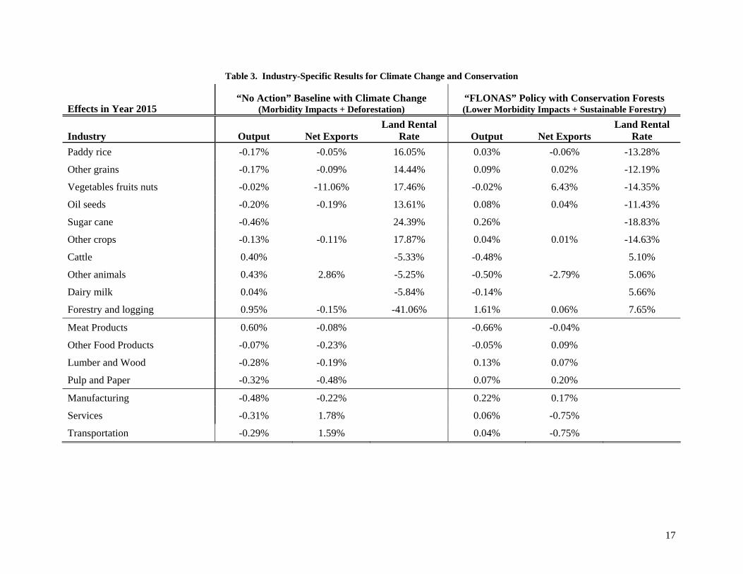
Table 3. Industry-Specific Results for Climate Change and Conservation

Effects in Year 2015 “No Action” Baseline with Climate Change

(Morbidity Impacts + Deforestation) “FLONAS” Policy with Conservation Forests (Lower Morbidity Impacts + Sustainable Forestry)

Industry Output Net Exports Land Rental

Rate Output Net Exports Land Rental

Rate Paddy rice -0.17% -0.05% 16.05% 0.03% -0.06% -13.28%

Other grains -0.17% -0.09% 14.44% 0.09% 0.02% -12.19%

Vegetables fruits nuts -0.02% -11.06% 17.46% -0.02% 6.43% -14.35%

Oil seeds -0.20% -0.19% 13.61% 0.08% 0.04% -11.43%

Sugar cane -0.46% 24.39% 0.26% -18.83%

Other crops -0.13% -0.11% 17.87% 0.04% 0.01% -14.63%

Cattle 0.40% -5.33% -0.48% 5.10%

Other animals 0.43% 2.86% -5.25% -0.50% -2.79% 5.06%

Dairy milk 0.04% -5.84% -0.14% 5.66%

Forestry and logging 0.95% -0.15% -41.06% 1.61% 0.06% 7.65%

Meat Products 0.60% -0.08% -0.66% -0.04%

Other Food Products -0.07% -0.23% -0.05% 0.09%

Lumber and Wood -0.28% -0.19% 0.13% 0.07%

Pulp and Paper -0.32% -0.48% 0.07% 0.20%

Manufacturing -0.48% -0.22% 0.22% 0.17%

Services -0.31% 1.78% 0.06% -0.75%

Transportation -0.29% 1.59% 0.04% -0.75%

18

Following Jorgenson et al. (2004), health impacts associated with changes in infectious diseases are introduced into the CGE model via labor markets. The econometric estimates of health effects from Timmins (2003) and Pattanayak and Yasuoka (forthcoming) are translated into reductions in the effective stock of labor supply. To do this, we convert additional cases of morbidity into ‘healthy’ years lost due to disability (YLD) using WHO procedure. More specifically, YLD is the product of three variables: I - the number of incident cases in the reference period; DW - the disability weight, which ranges fro 0 to 1; and L - the average duration of disability (measured in weeks). I is available from the econometric model; DW are obtained from average values in the Global Burden of Disease Report (2002); and L reflects our best estimate of the number of weeks of disability for each disease. To convert this measure to a percentage change in labor endowments, we adjust this value by the share of population in the labor force. Collectively, these computations suggest an annual reduction in the Brazilian labor endowment of 0.47% because of climate change and of 0.39%, if climate change and associated disease incidence is mediated by FLONAS conservation.

In the CGE modeling, a “No Action” baseline is established that essentially includes the 0.47% reduction in available labor associated with climate change and higher rates of infectious diseases, along with future deforestation of roughly 3 million hectares of land per year (based on projections from Soares-Filho et al., 2006) – this land is assumed to enter agricultural land markets. This outcome is contrasted with a “FLONAS” policy that has a morbidity impact equal to 0.39% of the effective labor supply, along with additional sustainable timber production (which increases managed lands in Brazil by approximately 10 times).

The first several columns in Table 3 show how the “No Action” baseline compares to a hypothetical future in which no increases in temperatures or diseases occurs and deforestation continues into the future. Effects on industry output are generally negative, with the exception of some sectors benefiting from the additional land available as forests are cleared. The largest components of the economy, manufacturing and services (see Table 2), are negatively affected by interactions between climate change, infectious diseases, and the economy.

Table 4 gives macroeconomic results for GDP and other variables, along with a summary of the industry impacts. In general, the economy-wide implications of the “No Action” baseline and its associated climate change and diseases are negative.

Table 4. Macroeconomic Results for Climate Change and Conservation

Effects in Year 2015

“No Action” Baseline with Climate Change

(Morbidity Impacts + Deforestation)

“FLONAS” Policy with Conservation Forests

(Lower Morbidity Impacts + Sustainable Forestry)

GDP -0.20% 0.01% Consumption 0.03% -0.16% Investment -0.58% 0.33% Wage Rate 0.27% -0.07% Labor Earnings -0.23% 0.05% Exports -0.17% 0.05% Imports -0.12% 0.05% Output

Agriculture 0.01% -0.11% Energy -0.25% 0.08% Food 0.07% -0.18% Forestry/Wood -0.25% 0.15% Manufacturing -0.48% 0.22% Services -0.31% 0.06%

19

In the year 2015 shown, there is a minor increase in consumption as the economy adjusts to lower needs for capital in the future (and hence less need to invest today) – this effect on consumption is not present in future years. In comparison to the “No Action” case, we find that the FLONAS scenario results in higher GDP, lower wage rates, higher investment, higher imports and exports, declines in agriculture (as less land available) and increase in production of other industries. Again, the consumption finding for 2015 is a temporary phenomenon as people choose to invest more in the near term to prepare for higher levels of economic activity in the future.

We also conducted a preliminary assessment of the biodiversity gains from the forest protection scenario modeled in this paper. Specifically, we considers impacts on faunal biodiversity in the Amazon by overlaying the projected FLONAS scenario on the geographic range of endemic indicator species following the methodology used in Azevedo-Ramos et al. (2006). A summary of the methodology and details of the results are reported in Appendix B. This analysis shows that under the FLONAS scenario we can expect significant protection for some categories of species (see Table B-2), particularly for critically endangered mammals. Individual species would also gain varying increments in their protected range under this policy scenario (Table B-3 shows some examples). Further expansion of this type of analysis could identify the exact number of amphibians, mammals, and bird species that would be potentially prevented from extinction if these areas were protected.

VI. CONCLUSIONS AND FUTURE EXTENSIONS Ecosystems are the planet’s life support system. Why then is ecosystem degradation excessive or

so rapid? Unfortunately, the answer to this question is currently obscured by some conceptual confusion and lack of reliable data and methods for ecosystem valuation. We contend that provision of ecosystem services is sub-optimal because ecosystem services are public goods and ecosystem management involves externalities. These features also complicate efforts to develop credible estimates of ecosystem values because of limitations of appropriately scaled the data (often from other disciplines) and internally consistent methods. Consequently, policy makers lack good information to design and implement salient policies. We develop a case study for Brazil to illustrate how econometric estimation can be combined with computable general equilibrium (CGE) modeling to estimate ecosystem values associated with climate change and forest conservation. Econometric estimation with Brazilian regional data shows that climate change will increase morbidity (e.g., almost a 0.5% impact on labor endowment) and forest conservation can mediate climate impacts (by almost 20%). CGE simulations using econometric parameters suggest substantial economic impacts originating in land and labor markets. Preliminary biodiversity assessment suggests that for many species, which would otherwise lose 50% of their range, ecosystem protection represents insurance against future extinction risk. Thus, there is potential for significant ecosystem services (increased human welfare) via the disease regulation pathway, but much more research remains to be completed.

Future Extensions Like any modeling system, CGE models have limitations, among which are the use of poor

quality baseline data, inappropriate parameter values and inadequate modeling of land use dynamics (Angelson and Kaimowitz, 1995). The CGE model used here handles land use dynamics by including physical measures of land area, which are linked directly to crop production. However, opportunities exist to improve other aspects of the analysis. Foremost among these are the modeling of regional heterogeneity and disease dynamics.

There are several reasons to address regional differences or regionally disparate units. First, Brazil is a country of phenomenal heterogeneity in climate, biodiversity, health, landscape, urbanization, infrastructure, wealth, and education. The bias from aggregating or averaging these differences can be large. Second, there is an obvious interest in using this modeling to support policy decision making. It would be impossible to examine modifiable social stressors such as road building and the associated migration in a homogeneous model world. The spatial scale of the malaria, land use and deforestation is not the stumbling block to regional disaggregation.

20

Thus, it is our intention to extend the economic modeling to include multiple regions within Brazil. This can be accomplished most readily by combining the current national-level economic data provided by GTAP with data from IFPRI (Cattaneo, 2002), which are available for major sub-regions within Brazil (Amazon, Northeast, Center-west, South and Southeast). In addition to improving the current economic impact estimates, this level of disaggregation will facilitate future analyses of issues such as road expansion (following Cattaneo, 2001). A regional focus will also allow us to examine potential movements of people around the country in response to such changes. Migration in the model can be driven by economic factors such as wage differentials arising from changing economic activity (as the result of road expansions or changes in available agricultural land) and by other factors such as households reactions to disease rates (disutility from sickness or costs associated with morbidity or disease prevention).

Beyond regional dynamics, understanding and modeling malaria dynamics would greatly improve the analysis. Two recent papers (Gollin and Zimmermann, 2006; Chakraborty et al., 2007) provide key insights on how to incorporate dynamic epidemiological modeling into a CGE framework, in contrast to the illustrative structure used here. Our future plans include extending the CGE model to incorporate an explicit epidemiological model of malaria and linking it to population dynamics. As Gersovitz and Hammer (2005) illustrate, this implies using mathematical epidemiology (Wickwire, 1977) to characterize population changes in terms of births and deaths, which depend on the expenses for and effectiveness of prevention and therapy. Once this feature is include, disease rates in the model can then be tied to the wellbeing of Brazilian households by linking a malaria event to a utility cost (e.g., a DALY weight) and to a cost in terms of labor productivity. An explicit representation of the disease equilibrium also implies adding a health sector, in which firms provide prevention goods to households.

A major embellishment might also involve making malaria transmission probabilities conditional on modifications to vector habitat (due to deforestation) and migration, among other things. The final CGE framework would then be able to jointly consider multiple dimensions of a public road expansion project, for example: improved returns to deforested lands, higher paying jobs, improved access to health care in remote parts of the economy, and changes in malaria exposure. This ability to conduct integrated analysis within a unifying theoretical framework is what makes a CGE model into a comprehensive system for examining various modifiable social stressors such as policies to pay land owners for ecosystem services (ProAmbiente), widely viewed as the next big policy intervention in Brazil for ecosystem protection.

21

VII. REFERENCES: Angelsen, A., and D. Kaimowitz. 1995. “Rethinking the causes of deforestation: Lessons from economic

models.” The World Bank Research Observer, 14, pp.73-98. Angrist, J.D., G.W. Imbens, and D.B. Rubin, Identification of causal effects using instrumental variables.

Journal Of The American Statistical Association, 1996. 91(434): p. 444-455. Arrow, K.J., and G. Debreu. 1954. “Existence of an Equilibrium for a Competitive Economy.”

Econometrica 22:265-290. Ash, et al, 2006. Azevedo-Ramos, C., B., Domingues Do Amaral, D. C. Nepstad, B. Soares Filho, and R. Nasi 2006.

Integrating ecosystem management, protected areas and mammal conservation in the Brazilian Amazon. Ecology and Society 11(2): 17.

Brazilian National Institute for Space Research (INPE). 2006. “Estimativas Anuais Das Taxas de Desflorestamento da Amazônia Legal.” Available at: .http://www.obt.inpe.br/prodes/prodes_1988_2005.htm

Bruna, E. M., K. A. Kainer;, Philip M. Fearnside, William F. Laurance, Ana K. M. Albernaz, Heraldo L. Vasconcelos, and Leandro V. Ferreira. 2005. “Letters: A Delicate Balance in Amazonia.” Science (18 February): 1044-1045

Burniaux, J., and H. Lee. 2003. “Modeling land use changes in GTAP.” Centre for Global Trade Analysis. West Lafayette: Purdue University.

Câmara, G., A.P.D. Aguiar, Maria Isabel Escada, Silvana Amaral, Tiago Carneiro, Antônio Miguel Vieira Monteiro, Roberto Araújo, Ima Vieira, Bertha Becker. 2005. “Letters: Amazonian Deforestation Models.” Science 307 (18 February): 1043.

Carbone, J. and V.K. Smith. 2007. Evaluating Policy Interventions with General Equilibrium Externalities. Journal of Public Economics (in review).

Castilla, R. and D. Sawyer. 1993. “Malaria rates and fate: a socio-economic study of malaria and Brazil.” Social Science and Medicine 37(9): 1137-45.

Cattaneo, A. 2005. Inter-regional innovation in Brazilian agriculture and deforestation in the Amazon: income and environment in the balance. Environment and Development Economics. 10 (4): 485-511.

Cattaneo, A., 2002. “Balancing Agricultural Development and Deforestation in the Brazilian Amazon”. Research Report 129. International Food Policy Research Institute. Washington, D.C.

Cattaneo, A. (2001). "Deforestation in the Brazilian Amazon: Comparing the impacts of macroeconomic shocks, land tenure, and technological change." Land Economics 77(2): 219-240.

Chakraborty, S., C. Papageorgiou, et al. (2005). Disease and Development. LSU WP# 2005-12. Baton Rouge, LA, Lousiana State University

Corvalan C, Hales S, McMichael A et al (2005) Ecosystems and human well-being: health synthesis. A report of the Millennium Ecosystem Assessment.

Coxhead, I., and S. Jayasuriya. 1994. “Technical change in agriculture and land degradation in developing countries: A general equilibrium analysis.” Land Economics, 70(1), pp.20-37.

Cruz, W., and R. Repetto. 1992. The environmental effects of stabilization and structural adjustment programs: The Philippines case. Washington: World Resources Institute.

Darwin, R., M. Tsigas, J. Lewandrowski, and A. Raneses. 1995. World Agriculture and Climate Change: Economic Adaptations. Agricultural Economic Report No.703, Economic Research Service. Washington: US Department of Agriculture

Dasgupta, P., 2001. “Valuing Objects and Evaluating Policies in Imperfect Economies", Economic Journal, 2001, 111: (May), 1-29.

Devarajan, S. and S. Robinson. 2002. “The Influence of Computable General Equilibrium Models on Policy.” TMD Discussion Paper No. 98. Washington, DC: International Food Policy Research Institute (IFPRI).

22

Dee, P. 1991. “Modeling steady-state forestry in a Computable General Equilibrium context.” National Centre for Development Studies, Working Paper No.91/8. Canberra, Australia: The Australian National University.

Dimaranan, B.V. (Editor). 2006. Global Trade, Assistance, and Production: The GTAP 6 Data Base, Center for Global Trade Analysis, Purdue University.

FAO, 2005. “Food and Agriculture Indicators: Brazil.” Last Updated October, 2005. Freeman A (1996) On Valuing the Services and Functions of Ecosystems. In: Simpson and Christensen

(eds) Human Activity and Ecosystem Function: Reconciling Economics and Ecology, Chapman and Hall, New York.

Gersovitz, M. and J. S. Hammer (2005). "Tax/subsidy policies toward vector-borne infectious diseases." Journal of Public Economics 89(4): 647-674.

Gibb, T. 2005. “Deforestation of Amazon ‘Halved’” BBC News (August 26). Available at http://news.bbc.co.uk/go/pr/fr/-/2/hi/americas/4189792.stm

Goldsmith and Hirsch (2006). “The Brazilian Soybean Complex.” Choices 21(2):97-104. Gollin, D. and C. Zimmermann (2006). Malaria: Disease Impacts and Long-Run Income Differences.

WP# Williams College, Williams College. Golub, A., T. Hertel, H. Lee, and N. Navin Ramankutty. 2006. “Modeling land supply and demand in the

long run.” Centre for Global Trade Analysis. West Lafayette: Purdue University.

Heal GM, Barbier EB, Boyle KJ, Covich AP, Gloss SP, Hershner CH, Hoehn JP, Pringle CM, Polasky S, Segerson K, Shrader-Frechette K (2004) Valuing Ecosystem Services: Toward Better Environmental Decision Making. The National Academies Press, Washington, DC.

Jorgenson, D.W., R.J. Goettle, B.H. Hurd, and J.B. Smith. 2004. “U.S. market consequences of global climate change.” Pew Center on Global Climate Change, Arlington, VA.

Killeen, T.J. 2007. A Perfect Store in the Amazon Wilderness: Development and Conservation in the Context of the Initiative for the Integration of the Regional Infrastructure of South America (IIRSA). Applied Advances in Biodiversity Science, no. 7. Washington, DC: (CABS) Center for Applied Biodiversity Science at Conservation International (CI).

Kirby, K., W. Laurance, A. Albernaz, G. Schroth, P. Fearnside, S. Bergen, E. Venticinque, C. da Costa. 2006. “The Future of Deforestation in the Brazilian Amazon.” Futures. 38: 432-453.

Laurence, WF. PM. Fearnside, AKM Albernaz, HL Vasconcelos, and L. Ferreira. 2005. “Letters: Amazonian Deforestation Models.” Science 307 (18 February): 1044

Lee, H. 2004. “Incorporating agro-ecologically zoned land use data and landbased greenhouse gases emissions into the GTAP framework.” Centre for Global Trade Analysis. West Lafayette: Purdue University.

Lindsay, S.W., and M. Birley. 2004. Rural development and malaria control in Sub-Saharan Africa. EcoHealth 1: 129-137.

Margulis, S. 2004. “Causes of Deforestion of the Brazilian Amazon.” World Bank Working Paper No. 22. World Bank: Washington, D.C.

Martens, WJM. 1998. “Health Impacts of Climate Change and Ozone Depletion: An Ecoepidemiologic Modeling Approach”. Environmental Health Perspectives 106s:241-251.

McMichael, A.J., A. Haines, R. Sloof, and S. Kovats (1996), Climate Change and Human Health: An Assessment Prepared by a Task Group on Behalf of the World Health Organization, the World Meteorological Organization, and the United Nations Environment Programme, World Health Organization, Geneva.

Millennium Ecosystem Assessment (2005a) Ecosystems and Human Well-being: Biodiversity Synthesis. World Resources Institute, Washington DC.

23

Millennium Ecosystem Assessment (2005b) Chapter 6: Concepts of Ecosystem Value and Valuation Approaches. In: Ecosystems and Human Well-being: A Framework for Assessment.

Molyneux, D.. 2003. “Climate change and tropical disease: common themes in changing vector-borne disease scenarios.” Transactions of the Royal Society of Tropical Medicine and Hygeine 97: 129-132.

Nepstad, DJ, D. McGrath, A. Alencar, AC. Barros, G. Carvalho, M. Santilli, M. del C. Vera Diaz. 2002. “Frontier Governance in Amazonia”. Science 295: 629-631.

Pagiola S, Ritter K, Bishop J (2004) Assessing the Economic Value of Ecosystem Conservation. The World Bank Environment Department Paper No. 101, The World Bank, Washington DC.

Panayotou, T., and C. Sussangkarn. 1991. “The debt crisis, Structural adjustment and the environment: The case of Thailand.” Prepared for WWFN’s project on the Impact of Macroeconomic Adjustment on the Environment. London, UK: University of London.

Panayotou T (1992) The economics of environmental degradation: problems, causes and responses. In: Markandya and Richardson (eds) Environmental Economics: A Reader, St. Martin’s Press, New York.

Pattanayak, S.K., K. Dickinson, C. Corey, E.O. Sills, B.C. Murray, and R. Kramer. 2006a. “Deforestation, Malaria, and Poverty: A Call for Transdisciplinary Research to Design Cross-Sectoral Policies”. Sustainability: Science, Practice and Policy. 2(2): 1-12.

Pattanayak, S.K., M. T. Ross, B.M. Depro and C. Timmins. 2006b. “Biodiversity Conservation, Climate Change, and Human Health”. Presented at the Biodiversity and Human Health Workshop. U.S EPA and Yale University. Washington, DC, September.

Pattanayak SK, Butry DT (2005) Spatial Complementarity of Forests and Farms: Accounting for ecosystem services. American Journal of Agricultural Economics 87(4): 995-1008.

Pattanayak, S.K., and J. Yasuoka. Forthcoming. “Deforestation and Malaria: Revisiting the Human Ecology Perspective”. In C.J.P. Colfer (ed.), Human Health and Forests: A Global Interdisciplinary Overview. Earthscan Publishers.

Pattanayak SK (2004) Valuing watershed services: concepts and empirics from southeast Asia. Agriculture Ecosystems and Environment 104: 171-184.

Patz J, Confalonieri U et al (2005) Human Health: Ecosystem Regulation of Infectious Diseases. A report of the Millennium Ecosystem Assessment.

Patz, J.A., P. Daszak, G.M. Tabor, A.A. Aguirre, M. Pearl, J. Epstein, N.D. Wolfe, A.M. Kilpatrick, J. Foufopoulos, D. Molyneux, J.J. Bradley, and Members of the Working Group on Land Use Change and Disease Emergence. 2004. Unhealthy landscapes: policy recommendations on land use change and infectious disease emergence. Environmental Health Perspectives 112(10): 1092-1098.

Patz, JA, Graczyk, TK, Geller, N. and AY Vittor. 2000. “Effects of environmental change on emerging parasitic diseases.” International Journal for Parasitology 30(12-13): 1395-1405.

Patz, J.A., P. Epstein, T.A. Burke, and J.M. Balbus. 1996. “Global Climate Change and Emerging Infectious Diseases.” Journal of the American Medical Association 275(3):217-223.

Pfaff, A. 1999, “What Drives Deforestation in the Brazilian Amazon.” Journal of Envrionmental Economics and Management 37: 26-43.

Polasky S, Costello C, Solow A (2005) The economics of biodiversity. In: Maler, Vincent (eds) Handbook of Environmental Economics, Volume 3, New York, Elsevier.

Portela, R., and I. Rademacher. 2001. “A dynamic model of patterns of deforestation and their effect on the ability of the Brazilian Amazon to provide ecosystem services”. Ecological Modelling 143: 115 – 143.

24

Ross, M. 2005. “Documentation of the Applied Dynamic Analysis of the Global Economy (ADAGE) Model.” RTI Working Paper 05_01. <http://www.rti.org/adage>.

Ross., M. 2007a. “Applied Dynamic Analysis of the Global Economy Modeling of Greenhouse Gas Emissions Abatement Options.” U.S.Environmental Protection Agency, Climate Economics Branch of the Climate Change Division.

Ross., M. 2007b. “Incorporating Climate Change Impacts into the ADAGE Model.” U.S.Environmental Protection Agency, Climate Economics Branch of the Climate Change Division.

Ross, M.T., R.H. Beach, and B.C. Murray. 2004. “General Equilibrium Assessment of Regional Climate Change Policy.” Proceedings of the 2004 National IMPLAN User's Conference. Shepherdstown, WV, October 6-8, 2004.

Ross, M.T., B.C. Murray, R.H. Beach, and B.M. Depro. 2005a. “State-Level Economic Impacts of Global Climate Change Policies: Analysis of the Climate Stewardship Act of 2003.” Prepared for the Pew Center on Global Climate Change.

Ross, M.T., R.H. Beach, B.M. Depro, and B.C. Murray. 2005b. “Regulatory Impact Analysis for the Final Clean Air Interstate Rule.” Prepared for the U.S. Environmental Protection Agency, Office of Air Quality Planning and Standards.

Ross, M., Depro, B., and S. K. Pattanayak. Forthcoming. “Assessing the Economy-Wide Effects.” In Ecomarket: Costa Rica’s Experience with Payments for Environmental Services. G. Platais and S. Pagiola (eds.). World Bank, Washington D.C.

Schaeffer, R., RLV Rodrigues, WF Laurance, AKM Albernaz, PM. Fearnside, Heraldo L. Vasconcelos, and Leandro V. Ferreira. 2005. “Letters: Underlying Causes of Deforestion.” Science 307(18 February): 1046-1047.

Schnepf, R. et al. 2001. “Agriculture in Brazil and Argentina: Developments and Prospects for Major Field Crops.

Simon, M. and F. Garagorry. 2005. “The Expansion of Agriculture in the Brazilian Amazon.” Environmental Conservation. 32(3):203-212.

Soares-Filho, B., D. Nepstad, L. Curran, G. Cerqueira, R. Garcia, C. Ramos, E. Voll, A. McDonald, P. Lefebvre, and P. Schlesinger. 2006. “Letters: Modeling Conservation in the Amazon Basin.” Nature (23 March):520-523.

Thiele, R., and M. Wiebelt. 1993. “National and international policies for tropical rain forest conservation – A quantitative analysis for Cameroon.” Environmental and Resource Economics, 3, pp.501-531

Timmins, C. 2003. "Health and Climate Change in the Developing World: The Impact of Global Warming on Brazilian Morbidity Patterns". Working Paper. Yale University.

Veríssimo, A., Cochrane, M. & Souza Jr. C. 2002. National Forest in the Amazon. Science, ( 297) 1478. Walsh, JF., Molynneux, DH and MH Birley. 1993. “Deforestation: effects on vector-borne disease.”

Parasitology. 106: S55-S75. Wickwire, K., Mathematical models for the control of pests and infectious diseases: a survey. Theoretical

Population Biology, 1977. 11: p. 182-238. Wilson, ML. 2001. “Ecology and Infectious Disease.” In Ecosystem Change and Public Health J. Aron,

and J.A. Patz. (eds.) The Johns Hopkins University Press: Baltimore, MD: 285-291. World Health Organization (WHO). “Global Burden of Disease (GBD) 2002 Estimates.”

http://www.who.int/healthinfo/bodgbd2002/en/index.html Obtained July, 2006. World Health Organization (WHO). 2001. “National Burden of Disease Estimates: A Practical Guide.”

http://www.who.int/healthinfo/nationalburdenofdiseasemanual.pdf Xie, J., T. Panayotou and J. Vincent. 1996. “Computable General Equilibrium Models and the Analysis

of Policy Spillovers in the Forest Sector.” Environmental Discussion Paper No. 19. Harvard Institute for International Development (HIID) International Environmental Program (IEP). <http:www.hiid.harvard.edu/pub/other/ieppub/ieppub.html>

Yasuoka J, Levins R.(forthcoming). Impact of Deforestation and Agricultural Development on Anopheline Ecology and Malaria Epidemiology. American Journal of Tropical Medicine and Hygiene.

25

VIII. APPENDIX A. ECONOMETRIC ANALYSIS OF DEFORESTATION AND MALARIA2 In this appendix, we report on the results of an econometric analysis of the regional correlation of malaria, forest cover and protected areas. This analysis fed the labor supply parameters for the ‘FLONAS scenario’ in the CGE modeling.

Figure A-18. Malaria, Population, Deforestation and Forest Protection in Brazil

a. Malaria b. Population

c. Protected Areas (Amazon) d. Deforestation (Amazon)

As illustrated in Figure A-1, we use a cross-sectional data set of approximately 490 Brazilian microregions, each of which comprises of 1-12 municipios (counties). The malaria data come from the DATASUS (http://w3.datasus.gov.br/datasus/) and are reported in terms of 1000 inhabitants, representing hospital morbidity over the 1992–2000 period. Climate is represented by long-run temperature and rainfall (averaged over several years) in the 490 microregions, based on weather stations (approximately one per microregion). Census data (http://www.ibge.gov.br/) on housing, population, education levels, income, medical care (proxied by number of doctors and hospital beds) and infrastructure (percentage of households connected to water, sanitation, and all-weather roads) are for 1991. Forest cover and

2 The analysis reported in this appendix draws on some initial illustrative research reported in Pattanayak and

Yasuoka (forthcoming) and on-going research conducted by Subhrendu Pattanayak (RTI), Simone Bauch (NCSU and Imazon) and Danielle Celentano of Imazon (Amazon Institute for the People and Environment, Belem, Brazil). The malaria and census data were originally compiled by Timmins (2003).

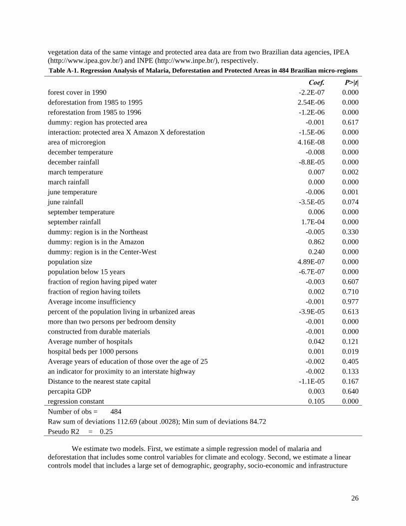
26

vegetation data of the same vintage and protected area data are from two Brazilian data agencies, IPEA (http://www.ipea.gov.br/) and INPE (http://www.inpe.br/), respectively. Table A-1. Regression Analysis of Malaria, Deforestation and Protected Areas in 484 Brazilian micro-regions

Coef. P>|t|forest cover in 1990 -2.2E-07 0.000deforestation from 1985 to 1995 2.54E-06 0.000reforestation from 1985 to 1996 -1.2E-06 0.000dummy: region has protected area -0.001 0.617interaction: protected area X Amazon X deforestation -1.5E-06 0.000area of microregion 4.16E-08 0.000december temperature -0.008 0.000december rainfall -8.8E-05 0.000march temperature 0.007 0.002march rainfall 0.000 0.000june temperature -0.006 0.001june rainfall -3.5E-05 0.074september temperature 0.006 0.000september rainfall 1.7E-04 0.000dummy: region is in the Northeast -0.005 0.330dummy: region is in the Amazon 0.862 0.000dummy: region is in the Center-West 0.240 0.000population size 4.89E-07 0.000population below 15 years -6.7E-07 0.000fraction of region having piped water -0.003 0.607fraction of region having toilets 0.002 0.710Average income insufficiency -0.001 0.977percent of the population living in urbanized areas -3.9E-05 0.613more than two persons per bedroom density -0.001 0.000constructed from durable materials -0.001 0.000Average number of hospitals 0.042 0.121hospital beds per 1000 persons 0.001 0.019Average years of education of those over the age of 25 -0.002 0.405an indicator for proximity to an interstate highway -0.002 0.133Distance to the nearest state capital -1.1E-05 0.167percapita GDP 0.003 0.640regression constant 0.105 0.000Number of obs = 484 Raw sum of deviations 112.69 (about .0028); Min sum of deviations 84.72 Pseudo R2 = 0.25

We estimate two models. First, we estimate a simple regression model of malaria and deforestation that includes some control variables for climate and ecology. Second, we estimate a linear controls model that includes a large set of demographic, geography, socio-economic and infrastructure

27

variables. To minimize the influence of outliers, we also estimate this model using quantile regression methods.

The key results are as follows. The naïve model (including some ecological controls for weather) is statistically significant and explains 46 per cent of the variation. First, we see that microregions with higher forest cover have lower rates of malaria, all things considered. Second, we find that microregions with higher deforestation (in the 1985–1995 time period) have greater rates of malaria. The linear controls model (where we account for potential confounding due to demographics, income, infrastructure and institutions, such as protected areas) is statistically significant and explains 56 per cent of the variation. First, we find that microregions with higher deforestation have greater rates of malaria – with a correlation that is significantly larger than the naïve model coefficients (almost twice as large). Second, microregions in the Amazon with conservation units have lower malaria rates for a given level of deforestation. This basic result is consistent across the OLS and quantile regression models.

These meso-scale data on malaria incidence, deforestation, road building, and migration limit causal inference because many of the social stressors underlying deforestation, migration etc. are not randomly assigned across the landscape. Instead, they reflect fundamental socio-economic and demographic phenomena that can mimic the risk factors and mask the ecological relationship of interest. The behavioral underpinnings of these phenomena pose classic confounding problems. Perhaps the best known remedy for this confounding problem is to apply the instrumental variable (IV) methodology (Angrist et al., 1996). Thus, we estimate an instrumental variable model.

The key to this strategy the identification of a natural experimental situation (e.g., a road building project) in which behavioral factors (e.g., determinants of road building) can serve as instruments for the ‘endogenous’ deforestation risk exposures. Thus, we estimate an IV model that which uses presence of protected area, distance to highway and to state capital, population, size and location of the microregion – as instruments for deforestation in the microregions. The overall IV model is significant. Now the deforestation coefficient is almost three times as big as for the linear-controls model. The results are consistent across the three models (i.e., deforestation is correlated with more malaria), but the sizes of the estimated coefficient are much larger (three- to sixfold) in the models that include proxies for human behavior.

Because our instrumental variable approach is exploratory and has not be subjected to tests for validity and strength, we rely on the results of the linear-controls model to generate disease impacts of conservation initiatives. The model parameters suggest that a 1 hectare decrease in deforestation would lower malaria rates by 8 per 1000. Thus, a country wide effort to reverse 3 million hectares of annual deforestation would imply a reduction in 1.41 million cases of malaria per year, given Brazil’s population of approximately 175 million.

28

IX. APPENDIX B. BIODIVERSITY ASSESSMENT3 A key factor in the selection of protected areas in the Brazilian Amazon is the number of

threatened species that are protected (Azevedo-Ramos et al. 2006). The goals of Brazil’s National System of Conservation Units (SNUC; law 9985 of 18 July 2000) include the maintenance of biological and genetic resources, the protection of threatened species, as well as to manage production forests and extractive reserves for sustainable livelihoods for Amazonian peoples. Avoiding extinction is also a goal in Brazil’s commitment to protect an additional 50 million hectares of forest in the Amazon through National Forests and other policy mechanisms (Soares-Filho, 2006). This reflects both the enormous potential value of the biological information stored in the earth’s richest storehouse of biodiversity, but also the irreversible nature of biodiversity loss. Unlike failure to secure human health, sustainable livelihood opportunities, climate change and hydrological cycles, a failure to avoid the extinction of the Amazon’s living species cannot be repaired by wiser policies later in the 21st century. The IUCN Red List is considered the most objective and authoritative measure of extinction risk (Lamoreux et al. 2003; Hambler 2004). For each of the mammals (Patterson et.al. 2003), birds (Birdlife, 2006) and amphibians (IUCN, 2006) listed as critically endangered, endangered or vulnerable in the Brazilian Amazon, we obtained the species geographic range from the most recently published sources. Weights for species were assigned with equal-steps’ described by Butchard et al. (2004, 2005, 2007). This is an ordinal ranking system, to assign specific values to threat status for multiple species with potentially overlapping spatial ranges. We chose the ‘equal-steps’ method over ranking systems with geometric weighting for higher threat classes because relatively few Amazonian species are under urgent extinction risk, recommending great attention to the avoidance of species entering into higher extinction threat categories. The ‘equal-steps’ method also leads to a more robust and representative index (Butchard et al. 1994). Following Barreto et al. (2006), we contend that protected areas will be located in areas of high deforestation risk from advancing economic frontiers and enabling road infrastructure. The areas under imminent deforestation risk are defined here as those areas shown by Barreto et al. (2006) to be under incipient human pressure, and outside the existing protected area system. They find that 19% of the Amazon is under threat from human settlements – indicators include deforested areas, urban zones, and agrarian reform settlements – and 28% is subject to incipient human pressure – in the form of fire zones or mining. For analytic purposes, the protected area system is here also considered to include military areas and indigenous areas. The areas at greatest risk of imminent deforestation and malarial emergence vary in the degree to which they might contribute to extinction avoidance. A spatial index of biodiversity importance was calculated for each 1km forest cell in the Legal Amazon outside the protected area system and under imminent deforestation risk. By selecting those unprotected cells under imminent deforestation risk with the highest values on the biodiversity index, we can examine the hypothetical contribution of the expansion of protected areas for human disease avoidance that would also reduce extinction risk.

While areas under pressure from incipient human pressure could be more costly to protect (Barreto et al. 2006), there are several reasons we choose to focus on these areas in our analysis. First, Capobianco et al. (2001) find that almost 50 percent of the priority areas for biodiversity conservation are outside of the protected areas system and these areas are under some type of human pressure. In addition, almost 30 percent of the areas identified as being economically attractive for sustainable logging in the Brazilian Amazon (Verissimo et al. 2000) are affected by some type of human pressure. Both of these studies indicate that we cannot simply ignore areas affected by human pressure if we want to protect threatened species or provide sustainable economic uses of natural resources. Protecting areas where human pressure is high, however, requires adequate management regimes. These would include public

3 The analysis reported in this appendix draws on research led by Keith Alger and Miroslav Honzak at Conservation

International’s Center for Applied Biodiversity Sciences.

29

production forests, sustainable development reserves, incentives rewarding compliance with ecological-economic zoning plans, and community conservation areas. In the zoning and management plans for production forests, areas internal to FLONAS and FLOTAS, with lower economic opportunity costs, can allow for biodiversity conservation objectives to be met. The biodiversity index of threatened species was calculated for the approximately 100 million ha of forested areas of the Brazilian Amazon outside the protected area system and under imminent deforestation risk. Selecting 50 million ha for protection according to their highest potential contribution to biodiversity conservation yields Table 1, showing the incremental area that might be gained for protection of threatened species. Since all IUCN threatened Amazonian Species occurring in Brazil exist in areas under imminent deforestation risk, all gain some habitat protection in this scenario. While further analysis is required of other taxa to confirm the enhanced conservation status provided to all Amazonian biodiversity, protection of areas for threatened vertebrates not only addresses threat to these species, but to those plants and invertebrates associated with them. Selecting for enhanced environmental management those areas that are under deforestation risk and also within the range of threatened species can add incalculable value of existence for all currently threatened Amazon species.

Table B-1. Percent of protection in policy scenario IUCN Red List categories Amphibians Mammals Birds 3 Kingdoms*

Full range (ha) - 65,021 - 65,021 50 million (ha) - 21,360 - 21,360

Critically endangered

% of range - 32.85% - 32.85% Full range (ha) - 11,111,159 4,023,404 11,326,888 50 million (ha) - 506,593 294,865 506,593

Endangered

% of range - 4.56% 7.33% 4.47% Full range (ha) 809,879 14,694,603 312,940 14,694,603 50 million (ha) 50,982 506,593 72,787 506,593

Vulnerable

% of total 6.30% 3.45% 23.26% 3.45% *Because of overlapping species ranges, 3 Kingdoms area is different than sum of area in IUCN category

Comparing the ‘additional’ protection that would be gained for species in the 50 million hectares selected in our analysis and the current protected areas system shows that for some categories of species significant increases would occur (Table 2). This is especially the case for critically endangered mammals.

Table B-2. Additional protection from policy scenario IUCN Red List categories Amphibians Mammals Birds 3 Kingdoms*

% of range in current PA system 11.09% 11.09% % of range protected in 50m scenario 32.85% 32.85%

Critically endangered

Total 43.94% 43.94% % of range in current PA system 15.99% 10.55% 15.78% % of range protected in 50m scenario 4.56% 7.33% 4.47%

Endangered

Total 20.55% 17.87% 20.25% % of range in current PA system 19.07% 13.89% 10.53% 13.89% % of range protected in 50m scenario 6.30% 3.45% 23.26% 3.45%

Vulnerable

Total 25.37% 17.34% 33.79% 17.34% *Because of overlapping species ranges, 3 Kingdoms area is different than sum of area in IUCN category

Individual species would also gain varying increments in their protected range under this policy scenario, with a few examples shown in Table 3. Species ranges protected in this scenario also show areas that would not be deforested in future years according to Soares-Filho et. al. (2006). Thus for many species which would otherwise lose 50% of their range, this addition to their area protected represents insurance against future extinction risk. Further expansion of this type of analysis could identify the exact

30

number of amphibians, mammals, and bird species that would be potentially prevented from extinction if these areas were protected.

Table B-3. Species protection Species Kingdom Red List Category % of range protected in

50 million hectares Atelopus spumarius Amphibian Vulnerable 6.30% Saguinus bicolor Mammal Critically endangered 32.85% Ateles marginatus Mammal Endangered 17.88% Chiropotes satanas Mammal Endangered 5.92% Dinomys branickii Mammal Endangered 9.33% Priodontes maximus Mammal Endangered 4.95% Pteronura brasiliensis Mammal Endangered 5.96%

References: Azevedo-Ramos, C., B., Domingues Do Amaral, D. C. Nepstad, B. Soares Filho, and R. Nasi 2006.

Integrating ecosystem management, protected areas and mammal conservation in the Brazilian Amazon. Ecology and Society 11(2): 17.

Barreto C., Souza Jr. C., Noguerón R., Anderson A., Salomão, R., (2006) Human Pressure on the Brazilian Amazon Forests. World Resources Institute

BirdLife International (2006) Species factsheets Downloaded from http://www.birdlife.org on 1/5/2007 This information is based upon, and updates, the information published in BirdLife International (2000) Threatened birds of the world. Barcelona and Cambridge, UK: Lynx Edicions and BirdLife International, and BirdLife International (2004) Threatened birds of the world 2004 CD-ROM. These sources provide the information for species accounts for the birds on the IUCN Red List. BirdLife International (2006) Species range maps.

Capobianco, J.P.R. (Coord.), A. Verissimo, A. Moreira, D. Sawyer, I. Dos Santos, L.P. Pinto. 2001. Biodiversidade na Amazônia Brasileira. Avalição e Açõnes Prioritárias para a Conservação, Uso Sustentável e Repatrição de Benefícios. Instituto Socioambiental; Estação Liberdade.

Hambler, C. 2004. Conservation. Cambridge: Cambridge University Press. IUCN website. Accessed 05 April, 2007. http://www.iucnredlist.org/ IUCN, Conservation International, and NatureServe. 2006. Global Amphibian Assessment.

<www.globalamphibians.org>. Downloaded on 4 May 2006 Lamoreux J.; Resit Akcakaya H.; Bennun L.; Collar N.J.; Boitani L.; Brackett D.; Brautigam A.; Brooks

T.M.; da Fonseca G.A.B.; Mittermeier R.A.; Rylands A.B.; Gardenfors U.; Hilton-Taylor C.; Mace G.; Stein B.A.; Stuart S. 2003. Value of the IUCN Red List. Trends in Ecology and Evolution 18, 214–215.

Patterson, B. D., G. Ceballos, W. Secherest, M. F. Tognelli, T. Brooks, L. Luna, P. Ortega, I. Salazar, and B. E. Young. 2003. Digital distribution maps of the mammals of the western hemisphere. Version 1.0. NatureServe, Arlington,Virginia, USA

Veríssimo, A., C. Souza Jr., and P. Amaral. 2000. Identificação de Âreas com Potencial para a Criação de Florestas Nacionais na Amazônia Legal. MMA. Brasília. Online at: http://www.imazon.org.br/upload/im_livros_010.zip (2/21/06).

Veríssimo, A., M. A. Cochrane, C. Souza Jr., and R. Salomão. 2002. Priority areas for establishing national forests in the Brazilian Amazon. Conservation Ecology 6(1): 4

Soares-Filho et al. 2006: ARPA expansion of PA network from 32% to 41% of total forest area – cites: Montiel, F. Programa Áreas Protegidas da Amazônia - ARPA. Resumo Executivo [on line] <http://www.mma.gov.br/port/sca/ppg7/doc/arpareex.pdf> (2004)