Climate Change Impacts

1

Climate Change Impacts

Klaus Keller [email protected]

Guiding Ques+ons

1.  How can climate change impact natural and human systems?

2.  What are projec+ons of climate change impacts?

3.  How uncertain are these projec+ons? 4.  How might the uncertainty about the

climate change impacts affect adapta+on decisions?

2

How can climate change impact natural and

human systems? 3

Example 1: The last millennium

4 IPCC FAR figure 6.10 (2007)

467

Chapter 6 Palaeoclimate

Figure 6.10. Records of NH temperature variation during the last 1.3 kyr. (a) Annual mean instrumental temperature records, identified in Table 6.1. (b) Reconstructions using multiple climate proxy records, identified in Table 6.1, including three records (JBB..1998, MBH..1999 and BOS..2001) shown in the TAR, and the HadCRUT2v instrumental temperature record in black. (c) Overlap of the published multi-decadal time scale uncertainty ranges of all temperature reconstructions identified in Table 6.1 (except for RMO..2005 and PS2004), with temperatures within ±1 standard error (SE) of a reconstruction ‘scoring’ 10%, and regions within the 5 to 95% range ‘scoring’ 5% (the maximum 100% is obtained only for temperatures that fall within ±1 SE of all 10 reconstructions). The HadCRUT2v instrumental temperature record is shown in black. All series have been smoothed with a Gaussian-weighted filter to remove fluctuations on time scales less than 30 years; smoothed values are obtained up to both ends of each record by extending the records with the mean of the adjacent existing values. All temperatures represent anomalies (°C) from the 1961 to 1990 mean.

“Little Ice

Age”

Effects of the Little Ice Age on the Montenvers glacier, Mont Blanc region

http://www.swisseduc.ch/glaciers/glossary/little-ice-age-two-en.html

Little Ice Age maximum (~1730) Year 2000

http://www.pbs.org/saf/1505/features/heights.htm, Data obtained from "New Light on the 'Dark Ages'" by Richard H. Steckel in Social Science History.

“During the LIA, summers were wet and unusually cold and the growing season was shortened. Widespread crop failure resulted in famine that killed millions of people. To avoid starva+on, people would eat the plan+ng seed for next season, which created more of a shortage the following year.”

http://www.pbs.org/saf/1505/features/lia.htm

Social and Economic Impacts of the Little Ice Age (LIA)

Example Impact 2: Agriculture

7

How might climate change affect agricultural yields?

Photo by and (c) 2007 Derek Ramsey

8

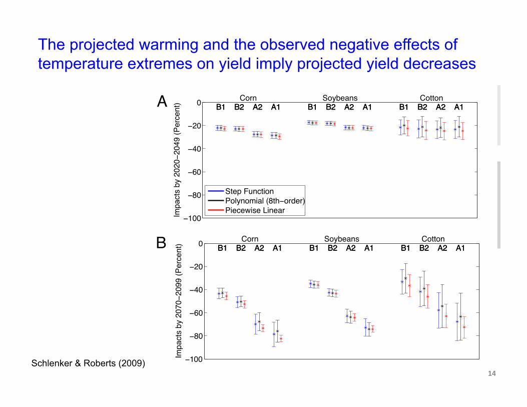
Schlenker & Roberts (2009)

approximately 1% difference in average yield for the year. Forexample, the blue line frame A (the flexible model for corn),substituting a full day (24 h) at 29° C temperature with a full dayat 40° C temperature results in a predicted yield decline of !7%,holding all else the same. The green histogram shows the averageexposure to each one-degree Celsius interval during the growingseason (March–August for corn and soybeans and April–October for cotton).

Coefficients on other explanatory variables (precipitation,squared precipitation, county fixed effects, and state-specificquadratic time trends) are not reported here. Precipitation hasa statistically significant inverted-U shape with an estimatedyield-maximizing level of 25.0 inches for corn and 27.2 inches forsoybeans in the flexible step-function specification in Fig. 1. Theprecipitation variables are not statistically significant for cotton,which is not surprising given that 58% of the crop is irrigated.Fixed effects control for time-invariant heterogeneity (like soilquality) and state-specific quadratic time trends control fortechnological change. With wide geographic variation in averageyields and a three-fold increase in yields over the sample period,these controls have strong statistical significance.

The pattern of temperature effects is quite robust to specifi-cation and controls. The same nonlinear temperature effectemerges whether or not any of the controls, or any subset ofcontrols, are included in the regressions. We also find theestimated temperature effects to be very similar if we insteadcontrol for technology and time effects by using year-fixedeffects rather than state-specific quadratic time trends.

Holding Current Growing Regions Fixed, Area-Weighted AverageYields Are Predicted to Decrease by 30–46% Before the End of theCentury Under the Slowest Hadley III Warming Scenario (B1), andDecline by 63–82% Under the Most Rapid Warming Scenario (A1FI).For comparison, a linear model that uses the average growing-season temperature as an explanatory variable gives predictedimpacts of "16% to #3% (B1) and "30% to #6% (A1FI)among the three crops. Yield predictions are summarized in Fig.2. Frame A shows predictions for the medium term (2020–2049)and frame B for the long term (2070–2099). Predictions are forchanges in total production under four climate scenarios in theHadley III climate model. Across all scenarios, model specifi-cations, and crops, the aggregate impacts show marked declines,even though yields in some individual counties are projected toincrease. The driving force behind these large and significantpredicted impacts is the projected increase in frequency ofextremely warm temperatures.

Out-of-Sample Model Predictions Are More Accurate than PreviousStatistical Models. The new regression models were comparedwith other specifications in the literature by using the root-meansquared error (RMS) of out-of-sample predictions. Each modelis estimated 1,000 times, randomly choosing 48 years of our56-year history of yields. The estimates are then used to predictyield outcomes for the remaining eight years (!14%) of eachsample. We randomly sample whole years and not observationsbecause yields are spatially correlated in any given year. Wecompare our own three specifications of temperature effects(step function, polynomial, and piecewise linear) with threealternative specifications: (i) a model with average temperaturesfor each of four months (1); (ii) an approximation of growing-degree days based on monthly average temperatures (Thom’sformula) (4); and (iii) a measure of growing-degree days,calculated by using daily mean temperatures (8), that does notinclude a separate category for extremely warm temperatures.

As a baseline, we consider a model with county-fixed effects

0 5 10 15 20 25 30 35 40

−0.075

−0.05

−0.025

0

0.025

Temperature (Celsius)

Lo

g Yiel

d (Bu

shels

)

Corn

0

10 5

Expo

sure

(Day

s)

Step FunctionPolynomial (8th−order)Piecewise Linear

0 5 10 15 20 25 30 35 40

−0.075

−0.05

−0.025

0

0.025


Lo

g Yiel

d (Bu

shels

)

Soybeans

0

10 5

Expo

sure

(Day

s)


0 5 10 15 20 25 30 35 40

−0.075

−0.05

−0.025

0

0.025


Lo

g Yiel

d (Ba

les)

Cotton

0

10 5

Expo

sure

(Day

s)


A B C

Fig. 1. Nonlinear relation between temperature and yields. Graphs at the top of each frame display changes in log yield if the crop is exposed for one day toa particular 1° C temperature interval where we sum the fraction of a day during which temperatures fall within each interval. The 95% confidence band, afteradjusting for spatial correlation, is added as gray area for the polynomial regression. Curves are centered so that the exposure-weighted impact is zero.Histograms at the bottom of each frame display the average temperature exposure among all counties in the data.

−100

−80

−60

−40

−20

0

Impa

cts by

2070−2

099 (

Perce

nt) B1 B2 A2 A1B1 B2 A2 A1B1 B2 A2 A1Corn

B1 B2 A2 A1B1 B2 A2 A1B1 B2 A2 A1Soybeans

B1 B2 A2 A1B1 B2 A2 A1B1 B2 A2 A1Cotton

−100

−80

−60

−40

−20

0

Impa

cts by

2020−2

049 (

Perce

nt)

B1 B2 A2 A1B1 B2 A2 A1B1 B2 A2 A1Corn




A

B

Fig. 2. Predicted climate-change impacts on crop yields under the Hadley IIIclimate model. Graphs display predicted percentage changes in crop yieldsunder four emissions scenarios. Frame A displays predicted impacts in themedium term (2020–2049) and frame B shows the long term (2070–2099). Astar indicates the point estimates, and whiskers show the 95% confidenceinterval after adjusting for spatial correlation. The color corresponds to theregression models in Fig. 1.

Schlenker and Roberts PNAS ! September 15, 2009 ! vol. 106 ! no. 37 ! 15595

ECO

NO

MIC

SCIE

NCE

SA

GRI

CULT

URA

LSC

IEN

CES

Observed yields decrease for extreme temperatures

Example Impact 3: Flooding

9

Flooding in the Netherlands in 1953 due to a storm surge

Source: National Archives and Records Administration, cataloged under the ARC Identifier (National Archives Identifier) 541705

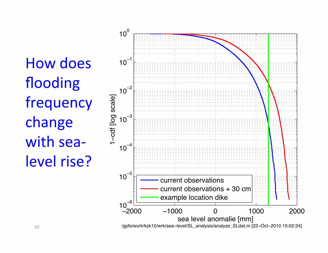
How does flooding frequency change with sea-‐level rise?

10

−2000 −1000 0 1000 200010−6

10−5

10−4

10−3

10−2

10−1

100

sea level anomalie [mm]

1−cd

f [lo

g sc

ale]

current observationscurrent observations + 30 cmexample location dike

/gpfs/work/kzk10/wrk/sea−level/SL_analysis/analyze_SLdat.m [22−Oct−2010 15:02:24]

Example 4: Heat waves

11 Picture: NASA, source: http://en.wikipedia.org/wiki/File:Canicule_Europe_2003.jpg

Heat waves are associated with increased mortality

12 IPCC, FAR, WGII, Figure C1.2 (2007)

What are projec+ons?

13

14

approximately 1% difference in average yield for the year. Forexample, the blue line frame A (the flexible model for corn),substituting a full day (24 h) at 29° C temperature with a full dayat 40° C temperature results in a predicted yield decline of !7%,holding all else the same. The green histogram shows the averageexposure to each one-degree Celsius interval during the growingseason (March–August for corn and soybeans and April–October for cotton).

Coefficients on other explanatory variables (precipitation,squared precipitation, county fixed effects, and state-specificquadratic time trends) are not reported here. Precipitation hasa statistically significant inverted-U shape with an estimatedyield-maximizing level of 25.0 inches for corn and 27.2 inches forsoybeans in the flexible step-function specification in Fig. 1. Theprecipitation variables are not statistically significant for cotton,which is not surprising given that 58% of the crop is irrigated.Fixed effects control for time-invariant heterogeneity (like soilquality) and state-specific quadratic time trends control fortechnological change. With wide geographic variation in averageyields and a three-fold increase in yields over the sample period,these controls have strong statistical significance.

The pattern of temperature effects is quite robust to specifi-cation and controls. The same nonlinear temperature effectemerges whether or not any of the controls, or any subset ofcontrols, are included in the regressions. We also find theestimated temperature effects to be very similar if we insteadcontrol for technology and time effects by using year-fixedeffects rather than state-specific quadratic time trends.

Holding Current Growing Regions Fixed, Area-Weighted AverageYields Are Predicted to Decrease by 30–46% Before the End of theCentury Under the Slowest Hadley III Warming Scenario (B1), andDecline by 63–82% Under the Most Rapid Warming Scenario (A1FI).For comparison, a linear model that uses the average growing-season temperature as an explanatory variable gives predictedimpacts of "16% to #3% (B1) and "30% to #6% (A1FI)among the three crops. Yield predictions are summarized in Fig.2. Frame A shows predictions for the medium term (2020–2049)and frame B for the long term (2070–2099). Predictions are forchanges in total production under four climate scenarios in theHadley III climate model. Across all scenarios, model specifi-cations, and crops, the aggregate impacts show marked declines,even though yields in some individual counties are projected toincrease. The driving force behind these large and significantpredicted impacts is the projected increase in frequency ofextremely warm temperatures.

Out-of-Sample Model Predictions Are More Accurate than PreviousStatistical Models. The new regression models were comparedwith other specifications in the literature by using the root-meansquared error (RMS) of out-of-sample predictions. Each modelis estimated 1,000 times, randomly choosing 48 years of our56-year history of yields. The estimates are then used to predictyield outcomes for the remaining eight years (!14%) of eachsample. We randomly sample whole years and not observationsbecause yields are spatially correlated in any given year. Wecompare our own three specifications of temperature effects(step function, polynomial, and piecewise linear) with threealternative specifications: (i) a model with average temperaturesfor each of four months (1); (ii) an approximation of growing-degree days based on monthly average temperatures (Thom’sformula) (4); and (iii) a measure of growing-degree days,calculated by using daily mean temperatures (8), that does notinclude a separate category for extremely warm temperatures.

As a baseline, we consider a model with county-fixed effects

0 5 10 15 20 25 30 35 40

−0.075

−0.05

−0.025

0

0.025


Lo

g Yiel

d (Bu

shels

)

Corn

0

10 5

Expo

sure

(Day

s)


0 5 10 15 20 25 30 35 40

−0.075

−0.05

−0.025

0

0.025


Lo

g Yiel

d (Bu

shels

)

Soybeans

0

10 5

Expo

sure

(Day

s)


0 5 10 15 20 25 30 35 40

−0.075

−0.05

−0.025

0

0.025


Lo

g Yiel

d (Ba

les)

Cotton

0

10 5

Expo

sure

(Day

s)


A B C

Fig. 1. Nonlinear relation between temperature and yields. Graphs at the top of each frame display changes in log yield if the crop is exposed for one day toa particular 1° C temperature interval where we sum the fraction of a day during which temperatures fall within each interval. The 95% confidence band, afteradjusting for spatial correlation, is added as gray area for the polynomial regression. Curves are centered so that the exposure-weighted impact is zero.Histograms at the bottom of each frame display the average temperature exposure among all counties in the data.

−100

−80

−60

−40

−20

0

Impa

cts by

2070−2

099 (

Perce

nt) B1 B2 A2 A1B1 B2 A2 A1B1 B2 A2 A1Corn



−100

−80

−60

−40

−20

0

Impa

cts by

2020−2

049 (

Perce

nt)

B1 B2 A2 A1B1 B2 A2 A1B1 B2 A2 A1Corn




A

B

Fig. 2. Predicted climate-change impacts on crop yields under the Hadley IIIclimate model. Graphs display predicted percentage changes in crop yieldsunder four emissions scenarios. Frame A displays predicted impacts in themedium term (2020–2049) and frame B shows the long term (2070–2099). Astar indicates the point estimates, and whiskers show the 95% confidenceinterval after adjusting for spatial correlation. The color corresponds to theregression models in Fig. 1.

Schlenker and Roberts PNAS ! September 15, 2009 ! vol. 106 ! no. 37 ! 15595

ECO

NO

MIC

SCIE

NCE

SA

GRI

CULT

URA

LSC

IEN

CES

The projected warming and the observed negative effects of temperature extremes on yield imply projected yield decreases

Schlenker & Roberts (2009)

15 IPCC FAR WGII, TS (2007)

over the Mediterranean Basin, and also over eastern and centralEurope and, to a lesser degree, over northern Europe even as farnorth as central Scandinavia [12.3.1]. Recruitment andproduction of marine fisheries in the NorthAtlantic are likely toincrease [12.4.7]. Crop suitability is likely to change throughoutEurope, and crop productivity (all other factors remainingunchanged) is likely to increase in northern Europe, and decreasealong the Mediterranean and in south-east Europe [12.4.7].Forests are projected to expand in the north and retreat in thesouth [12.4.4]. Forest productivity and total biomass are likelyto increase in the north and decrease in central and easternEurope, while tree mortality is likely to accelerate in the south[12.4.4]. Differences in water availability between regions areanticipated to become more pronounced: annual average runoffincreasing in north/north-west, and decreasing in south/south-east Europe (summer low flow is projected to decrease by up to50% in central Europe and by up to 80% in some rivers insouthern Europe) [12.4.1, 12.4.5].

Water stress is likely to increase, as well as the number ofpeople living in river basins under high water stress (highconfidence).Water stress is likely to increase over central and southernEurope. The percentage of area under high water stress is likelyto increase from 19% to 35% by the 2070s, and the number ofpeople at risk from 16 to 44 million [12.4.1]. The regions mostat risk are southern Europe and some parts of central and easternEurope [12.4.1]. The hydropower potential of Europe isexpected to decline on average by 6%, and by 20 to 50% aroundthe Mediterranean by the 2070s [12.4.8.1].

It is anticipated that Europe’s natural systems and biodi-versity will be substantially affected by climate change (veryhigh confidence). The great majority of organisms andecosystems are likely to have difficulty in adapting to climatechange (high confidence).Sea-level rise is likely to cause an inland migration of beachesand loss of up to 20% of coastal wetlands [12.4.2.], reducing thehabitat availability for several species that breed or forage in low-lying coastal areas [12.4.6]. Small glaciers will disappear andlarger glaciers substantially shrink (projected volume reductionsof between 30% and 70% by 2050) during the 21st century[12.4.3]. Many permafrost areas in theArctic are projected to dis-appear [12.4.5.]. In the Mediterranean, many ephemeral aquaticecosystems are projected to disappear, and permanent onesshrink and become ephemeral [12.4.5]. The northward expansionof forests is projected to reduce current tundra areas under somescenarios [12.4.4]. Mountain communities face up to a 60% lossof species under high-emissions scenarios by 2080 [12.4.3]. Alarge percentage of the European flora (one study found up to50%) is likely to become vulnerable, endangered or committedto extinction by the end of this century [12.4.6]. Options foradaptation are likely to be limited for many organisms andecosystems. For example, limited dispersal is very likely toreduce the range of most reptiles and amphibians [12.4.6]. Low-lying, geologically subsiding coasts are likely to be unable toadapt to sea-level rise [12.5.2]. There are no obvious climateadaptation options for either tundra or alpine vegetation [12.5.3].

The adaptive capacity of ecosystems can be enhanced by reduc-ing human stresses [12.5.3, 12.5.5]. New sites for conservationmay be needed because climate change is very likely to alter con-ditions of suitability for many species in current sites (withclimate change, to meet conservation goals, the current reservearea in the EU would have to be increased by 41%) [12.5.6].

Nearly all European regions are anticipated to be negativelyaffected by some future impacts of climate change and thesewill pose challenges to many economic sectors (very highconfidence).In southern Europe, climate change is projected to worsen con-ditions (high temperatures and drought) in a region already vul-nerable to climate variability. In northern Europe, climatechange is initially projected to bring mixed effects, includingsome benefits, but as climate change continues, its negative ef-fects are likely to outweigh its benefits [12.4].

Agriculture will have to cope with increasing water demand forirrigation in southern Europe due to climate change (e.g.,increased water demand of 2 to 4% for maize cultivation and 6to 10% for potatoes by 2050), and additional restrictions due toincreases in crop-related nitrate leaching [12.5.7].Winter heatingdemands are expected to decrease and summer cooling demands

Technical Summary

52

Figure TS-13. Characteristics of the summer 2003 heatwave: (a) JJAtemperature anomaly with respect to 1961-1990; (b-d) June, July,August temperatures for Switzerland; (b) observed during 1864-2003;(c) simulated using a regional climate model for the period 1961-1990;(d) simulated for 2071-2100 under the SRES A2 scenario. The verticalbars in panels (b-d) represent mean summer surface temperature foreach year of the time period considered; the fitted Gaussiandistribution is indicated in black. [F12.4]

The projected warming implies that heat-waves will become more common.

Documents

Climate Change Impacts