Climate Monitoring BulletinAustralia

Issue No. 195 April 2002

-2

-1.5

-1

-0.5

0

0.5

1

1.5

Tem

pera

ture

Ano

mal

y

1950 1955 1960 1965 1970 1975 1980 1985 1990 1995 2000

Australian autumn minimum temperature anomaly (°C) - 1950 to 2001

The Climate Monitoring Bulletin is prepared by the Australian Bureau ofMeteorology’s National Climate Centre. It is issued three to four weeksafter the end of each month.

Correspondence relating to the bulletin may be directed to:

Climate Analysis SectionNational Climate CentreBureau of MeteorologyGPO Box 1289KMelbourne, VIC 3001Australia

Phone: 03 9669 4527FAX: 03 9669 4678 or +61 3 9669 4678 (international)

If you use any of the information from this Climate Monitoring Bulletin,please identify "National Climate Centre, Bureau of Meteorology" as thesource.

Figure on the front cover : Australian average autumn (March - May) minimumtemperature anomalies (°C) - 1950 to 2001, with a linear trend superimposed. Theanomalies are calculated with respect to the 1961-1990 base period, and have beenobtained from a high quality temperature data set maintained by the National ClimateCentre.

© Commonwealth of Australia 2002Published by the Bureau of Meteorology, May 2002

1. General Circulation 1.1 General 1.2 Tropics 1.3 Extra-tropics

2. Oceanography 2.1 Surface 2.2 Subsurface

3. Australian Region 3.1 Overview 3.2 Rainfall 3.3 Rainfall Deficiencies 3.4 Temperatures 3.5 Outlook 3.6 Ozone

4. Australian National Tidal Facility Contribution

Tables1. Southern Oscillation and related climatic indices2. Australian ozone network report - February 2002

Figures1. Southern Oscillation Index2. Time series - 5 day running mean of equatorial 200 hPa velocity potential3. Time series - longitude plot of 200 hPa velocity potential4. 200 hPa velocity potential5a,b. Mean sea level pressure analysis and anomaly6a,b. 500 hPa geopotential height analysis and anomaly7a,b. Polar projection - mean sea level pressure analysis and anomaly8a,b. Polar projection - 500 hPa geopotential height analysis and anomaly9. Southern Hemisphere Blocking Index mean10. Southern Hemisphere Blocking Index - time longitude section11. 200 hPa Vector wind anomaly12. 850 hPa Vector wind anomaly13. Satellite derived sea surface temperature analysis14. Sea surface temperature anomaly15. Pacific depth averaged temperature to 150 m - Climatology16, 17. Pacific depth averaged temperature to 150 m - analysis and anomaly18. Pacific equatorial temperature section - Climatology 19, 20. Pacific equatorial temperature section - analysis and anomaly 21a,b. One month & three month rainfall deciles - Australia22a,b. Rainfall deficiencies - Australia23a,b. Maximum & minimum temperature anomaly - Australia24. Location of Australian Baseline Sea Level array25. Sea Level Anomalies26. Sea Level Residuals27. Hourly Wind Vectors

Contents

1.1 General

The Southern Oscillation Index (SOI) for April was –3.8, one point above the March value of –5.2.(1) The atmospheric and oceanic indices continued to indicate a largely neutral state, and themovement toward an El Niño observed in previous months appeared to stall. Recent values of theSOI are listed in Table 1 (at the end of this bulletin), along with related indices.

1.2 Tropics

1.2.1 MSLPs - Darwin and Tahiti

The average Mean Sea Level Pressure (MSLP) at Darwin for April was 1009.9 hPa, 0.4 hPa abovethe long-term average for the month. At Tahiti, the average MSLP for April was 1011.8 hPa,0.1 hPa below the long-term average. Monthly MSLP values were slightly below average acrossmuch of the tropical Pacific (see Figure 5(b)). Daily MSLP values for Tahiti oscillated around thelong-term average during the month, but Darwin’s values mostly stayed above climatologicalvalues (apart from the last week).

1.2.2 Winds and Walker Circulation

Low-level wind anomalies across the tropical Pacific were generally weak in April (Figure 12).There were some weak westerly anomalies in the far western tropical Pacific (around 140°E).Moderate upper-level wind anomalies were observed over the central to eastern tropical Pacific(Figure 11) in April.

1.2.3 Centres of Convection - Outgoing Longwave Radiation (OLR) and Velocity Potential (VP)

The monthly index of outgoing longwave radiation (OLR) in the region 160°E to 160°W and 5°Nto 5°S for April (not shown), obtained from the Climate Diagnostic Center in Washington, showeda return to positive values with no indication of a transition to El Niño-like values. High (low)index values are associated with reduced (increased) cloudiness in the specified area.

Figure 2 shows a filtered time series of 200 hPa velocity potential (VP) averaged from 5°N to 5°Sand 120°E to 140°E. Figure 3 is a time-longitude cross-section of 200 hPa VP averaged across 5°Nto 5°S for all longitudes. Little activity was evident in the index shown in Figure 2 for April, andindeed Figure 3 indicates that during mid-April the activity was mostly located further eastward,between 150 and 180°E.

The global 200 hPa VP for April is shown in Figure 4. The strongest minimum in the westernPacific region was located at the equator at around 170°E, just north of its March position. ForApril, this was northeast of its climatological position in the southern hemisphere. Minima indicatecentres of enhanced upper-level divergence and therefore increased convection in those regions.

1. General Circulation Features

(1) The Troup SOI used here has a standard deviation of +10.

Figure 1. Southern Oscillation Index

Figure 2. Time series plot of 5 day running mean 200 hPa Velocity Potential averaged from 5oN to 5oS and 120oE to 140oE. Units m2s–1

November December January February March April

-40

-30

-20

-10

0

10

20

30

Jan Jan Jan Jan Jan Jan Jan| | | | | | |

1996 1997 1998 1999 2000 2001 2002

Monthly SOI

weighted 5-month mean

Figure 3. Longitude - time series plot of 200 hPa Velocity potential (m2s–1),averaged over 5°S to 5°N. Data are smoothed with a 5 day running mean.

November

December

January

February

March

April

Figure 4. 200 hPa Velocity potential (m2s–1x106) for April 2002

Days

1.3 Extra-tropics

1.3.1 Pressure and height fields

Figures 5(a) and 5(b) show the global MSLP and MSLP anomaly maps respectively for April2002. The contour intervals are 5 hPa in Figure 5(a) and 2 hPa in Figure 5(b). Figures 6(a) and6(b) display the 500 hPa height and height anomaly maps. The contour intervals are 200 m and40 m respectively. These analyses are also provided in polar stereographic projections for theSouthern Hemisphere in Figures 7(a), 7(b), 8(a) and 8(b).

The polar trough for April showed three substantial pressure minima (Figure 7(a)) at 10°E, 100°Eand 150°W. In April, there were regions of anomalously low MSL pressure southeast of NewZealand and at the southern tip of South America. Another region of anomalously low pressure,though weak, was located at southwest of Australia. The main feature in the Australian region wasthe anomalous high south of Tasmania with higher than average pressure over most of the country,especially in the east.

The 500 hPa height field anomaly pattern (Figure 6(b)) showed negative anomalies at southeast ofNew Zealand and southwest of Australia, but positive anomalies over Australia.

1.3.2 Blocking Index

Figure 9 shows monthly mean Southern Hemisphere Blocking Index (BI) values calculated at the500 hPa level. Figure 10 is a time-longitude cross-section of the daily BI, calculated at the samelevel. The horizontal axes of Figures 9 and 10 show degrees of longitude east of the GreenwichMeridian. Blocking for the month was above average in the eastern longitudes and mostly belowaverage in the western longitudes. This can be seen in the previously mentioned disposition of themid-level height anomalies (Figure 6(b)).

1.3.3 Wind anomalies

Global vector wind anomalies at the 200 hPa and 850 hPa levels for April are shown in Figures 11and 12 respectively. In the low levels (Figure 12), two weak anomalous cyclonic circulations wereevident to the southeast of New Zealand and southwest of Australia respectively with adjacentanti-cyclonic circulation over the Southern Ocean between the two systems. Weak to moderatenorthwesterlies and northerlies were observed over Australia. In the upper levels (Figure 11), theabove anomalous circulations were also evident but the anti-cyclonic circulation was stronger.Another anomalous anti-cyclonic circulation centred over eastern Australia with strongernortheasterly and southwesterly flows was also observed.

Note: As foreshadowed in last month’s issue, Figures 2 to 12, obtained from the National Meteoro-logical and Oceanographic Centre’s Global Analysis and Prediction (GASP) system, are nowbased on daily 00UTC analyses. The April charts have been derived from the thirty 00UTC analy-ses for 1st April to 30th April. Prior to March, these charts were derived from 23UTC analyses.

Figure 5(a). Mean sea level pressure analysis (hPa) for April 2002

Figure 5(b). Mean sea level pressure anomaly (hPa) for April 2002

Figure 6(a). 500 hPa geopotential height (metres) for April 2002

Figure 6(b). 500 hPa geopotential height anomaly (metres) for April 2002

Figure 7(a). MSL pressure analysis (hPa) Figure 7(b). MSL pressure anomaly (hPa)

Figure 8(a). 500 hPa geopotential height (metres)

Figure 8(b). 500 hPa geopotential height anomaly(metres)

Polar projection - southern hemisphere

April 2002

April 1st

April 30th

Figure 9. Blocking Index (solid line). Ten year mean overlaid (dashed line).B.I. = 0.5 (U25 + U30 + U55 + U60 – U40 – U50 – 2U45)

Figure 10. Time-Longitude cross-section - daily Blocking Index.

Modeltime

(days)

Figure 11. 200 hPa vector wind anomaly (ms–1) for April 2002

Figure 12. 850 hPa vector wind anomaly (ms–1) for April 2002

Contour intervals are 5 ms–1 with shading starting at 5 ms–1 and becoming progessively darkerwith each interval.

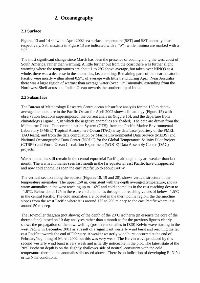
2.1 Surface

Figures 13 and 14 show the April 2002 sea surface temperature (SST) and SST anomaly chartsrespectively. SST maxima in Figure 13 are indicated with a "W", while minima are marked with a"C".

The most significant change since March has been the presence of cooling along the west coast ofSouth America, rather than warming. A little further out from the coast there was further slightwarming where the temperatures are about 1 to 2°C above average, but taken over NINO3 as awhole, there was a decrease in the anomalies, i.e. a cooling. Remaining parts of the near-equatorialPacific were mostly within about 0.5°C of average with little trend during April. Near Australiathere was a large region of warmer than average water (over +1°C anomaly) extending from theNorthwest Shelf across the Indian Ocean towards the southern tip of India.

2.2 Subsurface

The Bureau of Meteorology Research Centre ocean subsurface analysis for the 150 m depth-averaged temperature in the Pacific Ocean for April 2002 shows climatology (Figure 15) withobservation locations superimposed, the current analysis (Figure 16), and the departure fromclimatology (Figure 17, in which the negative anomalies are shaded). The data are drawn from theMelbourne Global Telecommunication System (GTS), from the Pacific Marine EnvironmentalLaboratory (PMEL) Tropical Atmosphere-Ocean (TAO) array data base (courtesy of the PMELTAO team), and from the data compilation by Marine Environmental Data Service (MEDS) andNational Oceanographic Data Center (NODC) for the Global Temperature-Salinity Pilot Project(GTSPP) and World Ocean Circulation Experiment (WOCE) Data Assembly Center (DAC)projects.

Warm anomalies still remain in the central equatorial Pacific, although they are weaker than lastmonth. The warm anomalies seen last month in the far equatorial east Pacific have disappearedand now cold anomalies span the east Pacific up to about 140°W.

The vertical section along the equator (Figures 18, 19 and 20), shows vertical structure in thetemperature anomalies. The upper 150 m, consistent with the depth averaged temperature, showswarm anomalies in the west reaching up to 1.6°C and cold anomalies in the east reaching down to–1.9°C. Below about 125 m there are cold anomalies throughout, reaching values of below –1.5°Cin the central Pacific. The cold anomalies are located in the thermocline region; the thermoclineslopes from the west Pacific where it is around 175 to 200 m deep to the east Pacific where it isaround 50 m deep.

The Hovmoller diagram (not shown) of the depth of the 20°C isotherm (in essence the core of thethermocline), based on 10-day analyses rather than a month as for the previous figures clearlyshows the propagation of the downwelling (positive anomalies in D20) Kelvin wave starting in thewest Pacific in December 2001 as a result of a significant westerly wind burst and reaching the fareast Pacific towards the end of February. A weaker westerly wind burst occurred at the end ofFebruary/beginning of March 2002 but this was very weak. The Kelvin wave produced by thissecond westerly wind burst is very weak and is hardly noticeable in the plot. The latest state of the20°C isotherm depth is on the slightly shallower side of neutral, consistent with the coldtemperature thermocline anomalies discussed above. There is no indication of developing El Niñoor La Niña conditions.

2. Oceanography

Figure 13. Blended sea surface temperature analysis (°C) for April 2002. (Source: National Meteorological and Oceanographic Centre)

Figure 14. Blended sea surface temperature anomaly (°C) for April 2002. (Source: National Meteorological and Oceanographic Centre)

Figure 17

Figure 16

Figure 15

Figure 20

Figure 19

Figure 18

3.1 Summary

April was warm across most of the country, with highest on record April monthly maximumtemperatures observed in many places. The warm conditions were accompanied by average tobelow average rainfall over much of the country.

3.2 Rainfall

The rainfall percentile analyses (deciles) use a reference period from 1900 to 2001 containingquality controlled data from the climate data bank. The data used for the rainfall percentileanalyses are based on preliminary real time data, which have not been verified and on which onlylimited quality control checks have been performed.

April

During April high pressure systems centred south of the Bight dominated the southern and easterncontinent, with the interspersed troughs from the heat low over northern WA and the cold frontsfrom the southern ocean lows causing the month’s rainfall. The only significant northern wetseason rainfall was during the second week when Tropical Cyclone Bonnie in the Timor Seacaused a moist northeast flow across the very top of the continent.

Around the country, April rainfall was mostly average to below average, with only a few areasrecording above average rainfall. The wet areas were mostly along the southern coast, and to amuch lesser extent the northern coast.

Below average (deciles 1 to 3) rainfall totals were widespread in the northern half of the country,with many smaller patches recording very much below average totals. Several small areas hadlowest-on-record totals. The dry conditions extended south along eastern parts of South Australiaand down to Tasmania, where the normally wet western half of the island experienced very muchbelow average April rainfall. Rainfall deciles for April 2002 are shown in Figure 21(a).

February to April

February to April conditions ranged from the very dry (in relative terms) in Tasmania and thesoutheastern half of South Australia, to the very wet in central Western Australia. A few places inTasmania and South Australia had lowest on record totals, while one part of central WA hadhighest on record February to April rainfall. Below average conditions extended across centralQueensland and down along the coast into northern New South Wales. Elsewhere in the country,the rainfall was patchy, with neither wet conditions nor dry conditions dominant. Rainfall decilesfor the three-month period February to April 2002 are shown in Figure 21(b).

3.3 Rainfall deficiencies

Rainfall deficiencies continued in northwest W.A., eastern Queensland and around theN.S.W./S.A./Victoria border region following average to below average falls during April. Thisthird area expanded extensively and a small area in the southeast of S.A. had the lowest rainfall onrecord for the five-month period from December to April (see Figure 22(a)).

There was also an intensification of the rainfall deficiencies near the east coast between Cooktownand Grafton, and an emergence of a region of serious deficiency on the northwest coast of

3. Australian Region

Figure 21(a)

Figure 21(b)

Figure 22(a)

Figure 22(b)

Tasmania over the three-month period beginning in February (see Figure 22(b)). Rainfalldeficiencies persisted in the far northern fringes of the Northern Territory.

3.4 Temperatures

Maximum temperature anomalies

April saw above average monthly maximum temperatures across most of the country, particularlyin the centre where a wide area recorded monthly anomalies in excess of +3°C. In some parts themonthly temperatures were more than 5°C above average. Many places in a broad belt straddlingthe Tropic of Capricorn experienced highest-on-record April monthly maximum temperatures. Afew very small areas on the northern and southern coasts recorded slightly below averagetemperatures. In area-averaged terms, this April was the warmest of the post-1950 period forQueensland, New South Wales, Tasmania, South Australia, the Northern Territory and Australia asa whole, the second warmest for Victoria (after April 1993) and the third warmest for WesternAustralia. The pattern of maximum temperature anomalies for April 2002 is shown in Figure23(a).

Minimum temperature anomalies

Most of the country also recorded above average minimum temperatures for April, although theanomaly pattern was less intense. A widespread area stretching from the northwest across thecentral south into the southeast of the continent recorded anomalies above +1°C. Around theSA/NSW/Qld border the minimum temperatures were more than 3°C above average. There weresome places however, mostly not too far from the coast, which recorded below average minimumtemperatures. In area-averaged terms, this April had the second highest monthly minimumtemperature of the post-1950 period for South Australia (after April 1961). The pattern ofminimum temperature anomalies for April 2002 is shown in Figure 23(b).

3.5 Outlook

The forecast model is based on the lagged statistical relationship between sea surface temperaturepatterns in the Indian and central to eastern tropical Pacific Oceans, and total seasonal rainfall aswell as seasonal mean maximum and minimum temperatures. The predictor inputs into the modelare derived from sea surface temperatures for February and April, with the ENSO SST patternshowing values of +0.732 and +1.299 respectively, and the Indian Ocean SST pattern showingvalues of +0.170 and +0.968 respectively. These values are expressed as standardised departuresfrom the mean, with positive departures indicating that the sea surface areas contributing to thepatterns have for the greater part positive anomalies.

Rainfall

Winter rainfall odds favour below average falls in an area straddling the NSW - Queensland bordercentred around Moree. For the June to August period, the chances of above average falls are lessthan 40% in this area, meaning that below average falls have a greater than 60% chance ofoccurring.

So with climate patterns like the current, about 6 winters out of 10 are expected to be drier thanaverage in this area, whilst about 4 out of 10 are wetter. In addition, based on historical data theoutlook scheme has moderate to good reliability through this region for winter.

Figure 23(a)

Figure 23(b)

Figure 23(a)

Figure 23(b)

Winter rainfall chances are also reduced across parts of the southeast and southwest of the country.However, in both these areas the outlook reliability is low so users are urged to interpret theprobabilities with caution. In other parts of the nation, the chances of above average winter rainfallare between 40 and 60% with no big swings to wet or dry conditions.

There continues to be speculation about a possible El Niño event this year. Despite a majority ofthe computer models surveyed predicting an event, the lack of supporting evidence from thePacific means the chance of an El Niño this year has decreased. The expert opinion fromAustralian climate scientists is that the odds for an El Niño event in 2002 have come back toaround 50%. This is still a significant chance, being roughly double the normal level of risk. If thepresent climate patterns persist for another month, the chance of an El Niño will be significantlylower because most El Niños are clearly established by the end of June.

As previously mentioned, the Outlook probabilities are based on recent Indian and Pacific Oceantemperatures. These probabilities have resulted from higher than average sea temperatures acrossmuch of the tropical Pacific and a warming of the Indian Ocean.

Temperature

Apart from the far north of the country, temperature odds clearly favour above averagetemperatures for winter. Over the June to August period the chances of above average seasonalmaximum temperatures are over 60% south of a line from Broome to Rockhampton, and theyapproach 80% across a large part of WA.

So with climate patterns like the current, about 7 winters out of every 10 are warmer than averageacross most of the country, with about 3 out of 10 being cooler. The outlook model has moderatereliability across much of the nation for winter.

The chances of above average seasonal minimum temperatures are in the 60 to 80% range overmuch of southern and western WA, and the outlook model has high reliability here. In other parts,the chances are between 40 and 60%.

SOI Analogues

The SOI analogues(1) for the nine months ending April suggest that the SOI will return to nearzero values during the June-August period, from its current weakly negative state. The compositepicture (not shown) formed by averaging the rainfall percentiles for the 8 post-1900 analogueperiods shows some tendencies towards drier than average conditions in southwest WA andsoutheastern coastal parts of the country (southern NSW, eastern Victoria and eastern Tasmania).There is little in the way of a consistent signal elsewhere in the country.

3.6 Ozone

Table 2 shows ozone data values, in Dobson units, for February 2002 for four Australian stations.The delay in the publishing of these data is due to the strict quality control procedures necessaryfor ozone data.

(1) The SOI analogues are calculated using a reconstructed time-series commencing from 1876. Monthly rainfall

analyses are only available from 1900 onwards.

4. Australian National Tidal Facility Charts

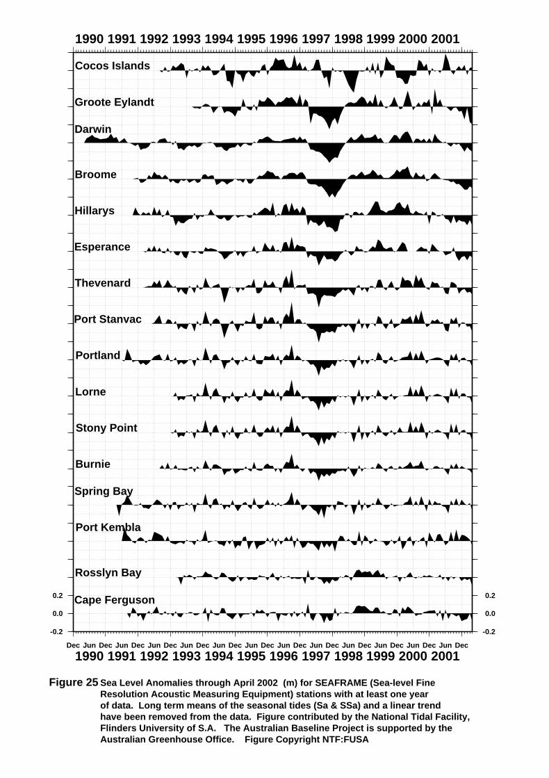
The National Tidal Facility (NTF), based at Flinders University, South Australia, supplies sea-leveland wind data from its measuring sites located around the Australian coastline and at Cocos Island.The locations of the various measuring stations are shown in Figure 24 with data being displayedin Figures 25 to 27.

The following remarks are based largely on a commentary supplied by the NTF.

NOTES ON THE DATA FOR APRIL 2002

Sea level data return this month was excellent at all stations.

The sea level anomalies (Figure 25) are negative at all sites except Cocos Islands. The anomaliesare substantial from Rosslyn Bay anti-clockwise to Thevenard.

The residuals (Figures 26), or difference between the observations and the tidal predictions, are thenon-tidal components of the sea level observations. The residuals are primarily the consequence ofshort-term meteorological effects (Figure 27) and may give the result of elevated or depressed sealevel observations.

100˚

100˚

110˚

110˚

120˚

120˚

130˚

130˚

140˚

140˚

150˚

150˚

160˚

160˚

-50˚ -50˚

-45˚ -45˚

-40˚ -40˚

-35˚ -35˚

-30˚ -30˚

-25˚ -25˚

-20˚ -20˚

-15˚ -15˚

-10˚ -10˚

-5˚ -5˚

0˚ 0˚

100˚

100˚

110˚

110˚

120˚

120˚

130˚

130˚

140˚

140˚

150˚

150˚

160˚

160˚

-50˚ -50˚

-45˚ -45˚

-40˚ -40˚

-35˚ -35˚

-30˚ -30˚

-25˚ -25˚

-20˚ -20˚

-15˚ -15˚

-10˚ -10˚

-5˚ -5˚

0˚ 0˚

100˚

100˚

110˚

110˚

120˚

120˚

130˚

130˚

140˚

140˚

150˚

150˚

160˚

160˚

-50˚ -50˚

-45˚ -45˚

-40˚ -40˚

-35˚ -35˚

-30˚ -30˚

-25˚ -25˚

-20˚ -20˚

-15˚ -15˚

-10˚ -10˚

-5˚ -5˚

0˚ 0˚

Port Kembla

Portland

Rosslyn Bay

Spring Bay

Port Stanvac

Thevenard

Burnie

BroomeCape Ferguson

Cocos Islands (Home Island) Darwin

Esperance

Hillarys

Standard SEAFRAME Gauges

Groote Eylandt (Milner Bay)

LorneStony Point

Customised SEAFRAME Gauges

Figure 24Figure 24 The Australian Baseline Sea Level and Climate Monitoring ProjectThe Australian Baseline Sea Level and Climate Monitoring Project

SEAFRAME (Sea-level Fine Resolution Acoustic Measuring Equipment) stations SEAFRAME (Sea-level Fine Resolution Acoustic Measuring Equipment) stations Figure contributed by the National Tidal Facility, Flinders University of S.A. TheFigure contributed by the National Tidal Facility, Flinders University of S.A. TheAustralian Baseline Project is supported by the Australian Greenhouse Office. Australian Baseline Project is supported by the Australian Greenhouse Office. Hillarys is 25 km north of Fremantle, W.A., Port Stanvac is 35km south of OuterHillarys is 25 km north of Fremantle, W.A., Port Stanvac is 35km south of OuterHarbor, Adelaide, S.A., Spring Bay is 4 km south of Triabunna, S.E. Tas.,Harbor, Adelaide, S.A., Spring Bay is 4 km south of Triabunna, S.E. Tas.,Rosslyn Bay is 5 km south of Yeppoon, Qld. and Cape Ferguson is 20km east ofRosslyn Bay is 5 km south of Yeppoon, Qld. and Cape Ferguson is 20km east ofTownsville, Qld. Thevenard is the port of Ceduna, S.A. Stony Point is locatedTownsville, Qld. Thevenard is the port of Ceduna, S.A. Stony Point is locatedin Western Port, Vic. and both Lorne and Stony Point are fully funded by the Portin Western Port, Vic. and both Lorne and Stony Point are fully funded by the Portof Melbourne Authority. The development of the gauge at Burnie, Tas. has been of Melbourne Authority. The development of the gauge at Burnie, Tas. has been assisted by the CSIRO Office of Space Science and Applications. The gauge onassisted by the CSIRO Office of Space Science and Applications. The gauge onCocos Island is located on Home Island and on Groote Eylandt the gauge is Cocos Island is located on Home Island and on Groote Eylandt the gauge is located on Milner Bay.

-0.2

0.0

0.2

0.4

0.6

0.8

1.0

1.2

1.4

1.6

1.8

2.0

2.2

2.4

2.6

2.8

3.0

3.2

3.4

3.6

3.8

4.0

4.2

4.4

4.6

4.8

5.0

5.2

5.4

5.6

5.8

6.0

6.2

-0.2

0.0

0.2

0.4

0.6

0.8

1.0

1.2

1.4

1.6

1.8

2.0

2.2

2.4

2.6

2.8

3.0

3.2

3.4

3.6

3.8

4.0

4.2

4.4

4.6

4.8

5.0

5.2

5.4

5.6

5.8

6.0

6.2

Cocos Islands

Groote Eylandt

Darwin

Broome

Hillarys

Esperance

Thevenard

Port Stanvac

Portland

Lorne

Stony Point

Burnie

Spring Bay

Port Kembla

Rosslyn Bay

Cape Ferguson

Dec Jun

1990Dec Jun

1991Dec Jun

1992Dec Jun

1993Dec Jun

1994Dec Jun

1995Dec Jun

1996Dec Jun

1997Dec Jun

1998Dec Jun

1999Dec Jun

2000Dec Jun

2001Dec

1990 1991 1992 1993 1994 1995 1996 1997 1998 1999 2000 2001

Figure 25 Sea Level Anomalies through April 2002 (m) for SEAFRAME (Sea-level FineResolution Acoustic Measuring Equipment) stations with at least one yearof data. Long term means of the seasonal tides (Sa & SSa) and a linear trendhave been removed from the data. Figure contributed by the National Tidal Facility,Flinders University of S.A. The Australian Baseline Project is supported by the Australian Greenhouse Office. Figure Copyright NTF:FUSA

1 2 3 4 5 6 7 8 9 10 11 12 13 14 15 16 17 18 19 20 21 22 23 24 25 26 27 28 29 30

April 2002 (UTC)

-0.20.00.2

Cape FergusonCape Ferguson

-0.20.00.2

Rosslyn BayRosslyn Bay

-0.20.00.2

Port KemblaPort Kembla

-0.20.00.2

Spring BaySpring Bay

-0.20.00.2

BurnieBurnie

-0.20.00.2

Stony PointStony Point

-0.20.00.2

Lorne

-0.20.00.2

PortlandPortland

-0.20.00.2

Port StanvacPort Stanvac

-0.20.00.2

ThevenardThevenard

-0.20.00.2

EsperanceEsperance

-0.20.00.2

HillarysHillarys

-0.20.00.2

BroomeBroome

-0.20.00.2

DarwinDarwin

-0.20.00.2

Groote EylandtGroote Eylandt

1 2 3 4 5 6 7 8 9 10 11 12 13 14 15 16 17 18 19 20 21 22 23 24 25 26 27 28 29 30

-0.20.00.2

Cocos IslandsCocos Islands

Figure 26 Six Minute Sea Level Residuals (m) from SEAFRAME (Sea-level Fine ResolutionAcoustic Measuring Equipment) stations for April 2002. Residuals are thedifferences between the sea level observations and the predicted astronomicaltide. Figure contributed by the National Tidal Facility, Flinders Universityof S.A. The Australian Baseline Project is supported by the Departmentof the Environment, Sport and Territories. Figure Copyright NTF:FUSA

1 2 3 4 5 6 7 8 9 10 11 12 13 14 15 16 17 18 19 20 21 22 23 24 25 26 27 28 29 30

April 2002 (UTC)

-10

0

10

15 m/s15 m/s

Cape FergusonCape Ferguson

-10

0

10

Rosslyn BayRosslyn Bay

-10

0

10

Port KemblaPort Kembla

-10

0

10

Spring BaySpring Bay

-10

0

10

BurnieBurnie

-10

0

10

Stony PointStony Point

-10

0

10

PortlandPortland

-10

0

10

Port StanvacPort Stanvac

-10

0

10

ThevenardThevenard

-10

0

10

EsperanceEsperance

-10

0

10

HillarysHillarys

-10

0

10

BroomeBroome

-10

0

10

DarwinDarwin

-10

0

10

Groote EylandtGroote Eylandt

1 2 3 4 5 6 7 8 9 10 11 12 13 14 15 16 17 18 19 20 21 22 23 24 25 26 27 28 29 30

-10

0

10

Cocos IslandsCocos Islands

Figure 27 Hourly Incident Winds (m/s, deg True) from SEAFRAME (Sea-level FineResolution Acoustic Measuring Equipment) stations for April 2002. Thevectors, pointing from the origin, indicate the direction from which the wind isblowing. Figure contributed by the National Tidal Facility, Flinders Universityof S.A. The Australian Baseline Project is supported by the Departmentof the Environment, Sport and Territories. Figure Copyright NTF:FUSA

Table1. Southern Oscillation and other related climatic indices.

SE IndianSOIAnomTahitiAnomDarwinMonthYearOcean(Troup)MSLPMSLPSSTusing a 60 year(hPa)(hPa)

Anombase 1933-1992

0.96-3.8-0.11011.80.41009.9Apr020.77-5.20.31011.91.31008.9Mar020.477.71.61012.70.01006.5Feb020.372.71.41012.30.91007.3Jan02

0.51-9.1-1.41009.50.41007.8Dec010.397.20.81012.5-0.31008.5Nov010.59-1.9-1.01012.6-0.71010.0Oct010.871.40.01014.4-0.21011.8Sep011.12-8.9-0.81013.70.61013.4Aug011.02-3.0-0.21013.90.31013.4July010.891.8-0.51013.4-0.51012.0June010.37-9.00.01012.61.11012.1May010.340.3-0.31011.6-0.31009.2Apr01-0.346.71.21012.80.01007.6Mar01-0.4411.9-0.41010.7-2.91003.6Feb01-0.038.92.61013.50.81007.2Jan01

0.197.7-1.11009.8-2.61004.8Dec000.4022.41.31013.0-2.11006.7Nov000.599.70.21013.8-1.41009.3Oct000.809.91.71016.10.11012.1Sep000.755.30.31014.8-0.51012.3Aug000.82-3.7-0.61013.50.01013.1July000.98-5.50.21013.90.91013.4June000.663.61.01013.60.51011.5May000.6416.80.81012.7-1.21008.3Apr000.329.41.51013.1-0.21007.4Mar000.5712.92.71013.80.01006.5Feb001.025.11.31012.20.31006.7Jan00

0.8712.81.81012.7-0.71006.7Dec990.8413.11.31013.0-0.71008.1Nov990.279.11.21014.8-0.31010.4Oct990.04-0.40.41014.70.41012.4Sep990.362.11.51015.91.11013.9Aug990.614.80.91014.90.11013.2July990.831.00.61014.30.51013.0June990.731.31.31013.91.11012.1May990.7118.51.31013.2-0.91008.6Apr990.328.90.31011.9-1.31006.3Mar99-0.608.61.41012.5-0.41006.1Feb99-0.7215.61.81012.7-1.41005.0Jan99

-0.5113.31.01011.9-1.61005.8Dec980.0312.50.51012.2-1.41007.4Nov980.1410.90.81014.4-1.01009.7Oct980.6711.11.51015.9-0.31011.7Sep980.839.81.61016.00.01012.8Aug980.8214.61.61015.7-0.61012.5July980.959.90.91014.6-0.31012.2June981.500.50.61013.20.51011.5May98

Table 2: Australian Ozone Network Report for February 2002

NOTES

MEAN - Monthly mean total ozone.

MAX - Maximum daily total ozone value for the month.

MIN - Minimum daily total ozone value for the month.

L.T. MEAN - Long term mean based on data from previous years where available

L.T. MAX - Highest monthly mean obtained from previous years’ records

L.T. MIN - Lowest monthly mean obtained from previous years’ records

* All total ozone values expressed in Dobson Units.

** The results above include data which must be considered preliminary.

Station Mean Max Min L.T. Mean L.T. Max L.T. MinDarwin 256 274 234 247 256 239Brisbane 264 276 250 265 274 249

Melbourne 277 325 255 273 285 257Macquarie Island 281 308 249 292 314 276