CLIMATE PATTERN RECOGNITION IN THE LATE-TO … · CLIMATE PATTERN RECOGNITION IN THE LATE-TO-END ... half-wave cycle commenced in 8108 BC, ... 1. INTRODUCTION This 500 year period

CLIMATE PATTERN RECOGNITION IN THE LATE-TO-END

HOLOCENE (1600 AD TO 2050 AD, PART 8) JOACHIM SEIFERT

FRANK LEMKE

Correspondence to: [email protected]

Website: hKp://www.knowledgeminer.eu • hKp://www.climateprediction.eu

JANUARY 2018

©2018 Joachim Seifert

mailto:[email protected]

http://www.knowledgeminer.eu

http://www.climateprediction.eu

Climate pa3ern recognition in the late-to-end Holocene (1600 AD to 2050 AD)

Abstract. The time span 1600-2050 AD covers the most recent of a total of 30 cyclic sine half-wave periods, which developed since the beginning of the Holocene. The first half-wave cycle commenced in 8108 BC, with a periodicity of 238 years, see this series, paper part 1. This cycle is a growing cycle, which increments by 6.93 years, as all papers of the Holocene Climate PaKern Recognition analysis demonstrate. The present periodicity of the cycle is 439 years long, starting within the LiKle Ice Age (LIA) temperature boKom trough, 1590 to 1640 AD, at 1610 AD, and rising to the Current Warm Period (CWP) cycle top at 2049 AD. This Holocene paper series additionally serves as a 10,000 year empirical confirmation of astronomical-physical calculations of the cyclic nature of the climate in (Seifert, J. 2010). We showed that well-defined, regular wave periodicities led us out from the 500 BC Homerian Minimum into the Roman Warm Period, into the Late Antique LiKle Ice Age (LALIA) cold period, then into the Medieval Warm Period (MWP), followed by the cold LIA and now into the present warm CWP with its peak in 2049 AD and, thereafter, into the return of the next cold future “LIA”. As in seven previous recognition papers before, which cover the entire Holocene since 8500 BC, our obligatory paKern recognition grid was placed onto this time span 1600-2050 AD. We provide a comparison of nominal cyclic half-wave temperatures to actual measured GISP2 and GISS temperatures. It is demonstrated that the sine wave motion is modified by pulsations of the 62-year cosmic Solar-Planetary Oscillation (SPO; in previous parts called SIM) cycle (with the Atlantic Multidecadal Oscillation (AMO) and the Pacific Decadal Oscillation (PDO) as two observable oceanic temperature effects), which produces regularly spaced, consistent warm peaks along the entire Holocene (see this series, part 7). These warm peaks appear since 1818 AD in shapes of 4 upward moving staircase steps. The present staircase temperature peak is 2004 AD, from where on the flat step surface (today known as “The Pause”, “Hiatus”, “Plateau”) will persist until the year 2046 AD. The top of the sine wave temperature cycle is the year 2049 AD, from where on temperatures will enter into the 31st cycle, with a 439+6.93 year descent, until the future “LIA” temperature boKom will be reached. The final paper of this series, part 9, will cover the time span 2000 AD to the End of the Holocene. Such a forecast can be made, because existing five underlying cosmic, astronomical forcing mechanisms of climate change can be calculated. Citation. Seifert, J., Lemke, F.: Climate paKern recognition in the late-to-end Holocene (1600 AD to 2050 AD, part 8), 2018, hKp://www.knowledgeminer.eu/climate_papers.html

1. INTRODUCTION

This 500 year period is the most uncomplicated and straightforward period of the entire Holocene. It consists of a predominant half-sine wave periodicity, as the 30th cycle in the entire Holocene, rising out of the LIA boKom, starting 1610 AD, and rising to the new top, scheduled for 2049 AD. This sine wave was derived in detailed theoretical calculations in 2010 (Seifert, 2010), based on astronomical and physical parameters. Resulting in 30 cyclic climate half-waves continuing along the entire Holocene. The half-wave periodicity feature started in 8108 BC with a periodicity of 238 years, not in constant length, but as a growing periodicity, by 6.93 years for each period. For example, the 29th period, from 1177 AD to 1610 AD, thus reached 432 years in length. The periodicity initiation is explained in detail in part 1 of this series. Furthermore, all periodicities have a temperature amplitude, which is calculated by multiplying the cycle length with the factor 0.0037. The present sine half-wave periodicity is 439 years, which yields a temperature amplitude of 1.63°C on the GISP2 borehole temperature scale for the period ending in 2049 AD. Another feature is that upper and lower sine peaks show a secular Milankovitch temperature decline, which is 0.55°C/millennium for the lower sine peaks, and 0.51°C for the upper sine peaks. The overall secular temperature trend decline is 0.53°C/millennium, observed since the year 1 AD, which is demonstrated in the previous parts 6 and 7 of this series. We now proceed to the application of our climate paKern recognition grid.

2. PLACEMENT OF THE CLIMATE PATTERN RECOGNITION GRID

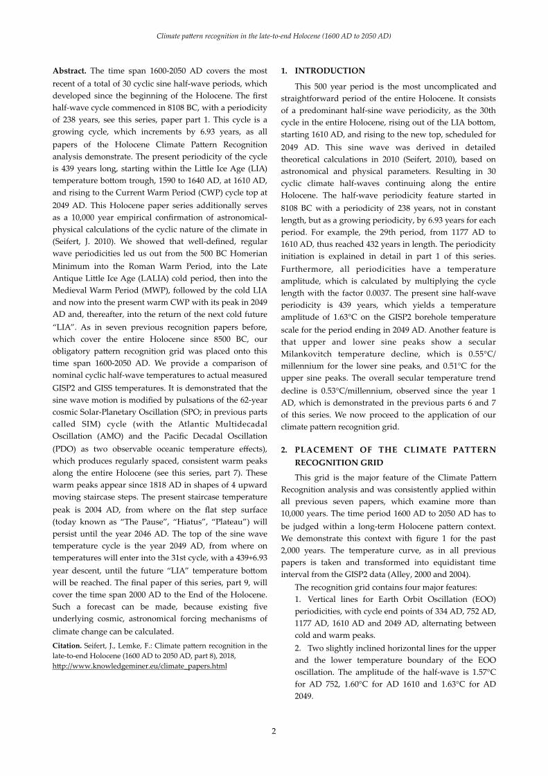
This grid is the major feature of the Climate PaKern Recognition analysis and was consistently applied within all previous seven papers, which examine more than 10,000 years. The time period 1600 AD to 2050 AD has to be judged within a long-term Holocene paKern context. We demonstrate this context with figure 1 for the past 2,000 years. The temperature curve, as in all previous papers is taken and transformed into equidistant time interval from the GISP2 data (Alley, 2000 and 2004).

The recognition grid contains four major features: 1. Vertical lines for Earth Orbit Oscillation (EOO) periodicities, with cycle end points of 334 AD, 752 AD, 1177 AD, 1610 AD and 2049 AD, alternating between cold and warm peaks. 2. Two slightly inclined horizontal lines for the upper and the lower temperature boundary of the EOO oscillation. The amplitude of the half-wave is 1.57°C for AD 752, 1.60°C for AD 1610 and 1.63°C for AD 2049.

�2

http://www.knowledgeminer.eu/climate_papers.html


3. The overall secular Milankovitch descent into the new glacial is 0.53°C/millennium. All temperatures are based on the GISP2 borehole temperature scale. 4. The solar 62-year Solar-Planetary Oscillation (SPO) pulsation, which produces robust temperature mini-peaks in an exact distance of 62 years within the entire Holocene is featured. Details of this cycle were given in the preceding, part 7 Holocene paper. We now place the grid onto this 1600-2050 AD

Holocene interval and arrive at the 30th period.

3. THE 30TH PERIOD (1610-2049 AD)

The situation for the 30th half-wave cycle is shown in figure 2.

Explanation: We establish a square design for this period and start with two vertical lines at 1610 AD and 2049 AD. To the horizontal lines: At the left boKom, there is the marker point of 1610 AD, with the value -32.08°C. as given in GISP2. The horizontal boKom line declines in a value of 0.55°C/millennium, which will yield a right boKom marker at -32.30°C. The upper left marker point for the horizontal line is 1.60°C above the -32.08°C position, thus a value of -30.50°C. The upper right marker point is 1.63°C above the boKom right of -32.30°C, thus located at -30.68°C, which produces an upper line descent of 0.51°C/millennium. The crosswise connection of the 4 marker points yields the center of the half-wave sine line, at 1830 AD. We add the GISP2 temperature measurement points and recognize immediately that massive ice build up and melt in the LIA substantially delayed global warming and kept the GISP2 temperature to much below

the nominal EOO temperature sine line. A helpful study on temperature evolution is the latest of MieKinen (MieKinen, 2015), presented in the Annex (fig. A1). In this study, in SE-Greenland, the EOO-LIA boKom trough as the boKom of the LIA, can very well be observed, both by the declining SST trend from 1300 AD onwards towards the temperature minimum trough 1590-1640 AD, and secondly, in the increasing sea ice cover extend from 1300 AD on, to its absolute maximum in the 1600-1620 AD trough, with 70-80% ice cover measured on the SE Greenland shelf. The EOO cold boKom trough produced shortened vegetation periods from 1590 to 1630, and subsequent grave famines in Europe within this time span occurred (see also Wikipedia, 2017).

Another frequently discussed aspect is the maximum temperature of the MWP, compared to the present ongoing CWP: According to the PaKern Recognition grid, the CWP top in 2049 AD lies at -30.68°C (in GISP2 borehole scale) and the MWP top is at -30.45°C, both close in height, the CWP top ranks slightly below the MWP. This agrees with figure 3, a maximum line, in (Ljungqvist, 2010), and agrees as well with (Moberg, 2005).

In order to utilize figure 2 for one additional feature, we introduce a horizontal line for the recent temperature plateau 2004-2017 AD, the “Global Warming Hiatus”, as described in (Medhang, 2017) with a hiatus trend of 0.005 +/- 0.146°C/decade. We introduce a second horizontal temperature plateau line from 1818-1858 AD. This line contains a volcano effect correction for twin volcano mega-eruptions 1808/09 (unidentified location — presumably Central America) and 1815 (Tambora). Both

�3

Figure 2. 30th half-wave cycle 1610 - 2049Figure 1. The past 2000 years of the Holocene


great eruptions lowered temperatures on Earth substantially, calculated in detail by (Stenni, 2017). The two mega-eruptions thus cut off the beginning part this second horizontal plateau line, which has to be restituted. The overall picture of cooling effects of volcanoes is given in (Sigl and Winstrup, 2015).

As next step, the introduction of the 62-year SPO cycle follows.

4. INTRODUCTION OF THE 62-YEAR SPO CYCLE

Global temperature evolution did not proceed directly along the nominal 30th sine half-wave line, because the fifth climate driving mechanisms, the 62-year SPO cycle, modifies the evolution line with consistent warm peaks. In the previous paper, Holocene part 7, we proved the consistency of this SPO cycle by demonstrating previous 62-year temperature peaks on a multi-millennial scale. This exact timing of warm peaks cannot be of tropospheric origin, because, using a Stocker quote: “The internal atmosphere-ocean climate system is unable to produce a forcing with a well-defined periodicity” (Stocker and Mysak, 1992). For this reason, this climate forcing is caused by solar - planetary oscillations (ScafeKa, 2013). For a 60+ year cycle of external forcing, the SPO cycle is the best candidate. We add the abstract conclusion made in the latest AMO study of (Murphy, 2017): “We conclude that there is an essential role for external forcing in driving the observed AMO”.

In order to demonstrate the cyclic nature of temperature peaks, we proceed from the Phil Jones Hadley staircase feature (fig. 3).

We observe stepwise temperature increases with flat plateaus in the 19th and 20th centuries. The shape of two l a s t s t e p w i s e i n c r e a s e s w e r e “ v i r t u a l l y indistinguishable” (May, 2016). The stepwise temperature increases and the 62-year cycle dates were entered into the recognition grid of figure 2 as displayed in figure 4.

The Evaluation of the time 1610 AD to, at first, 1794 AD: We observe that temperatures, after leaving the EOO trough with its minimum of -32.08°C remain flat and hover at about -32°C for almost 200 years. The GISP2

North Pole location appears insensitive to warming peaks, as discussed in the following point of the cooling effect of a large sea ice cover extent. The 62-year cycle has the warm peak dates of 2066 AD, 2004 AD, 1942 AD, 1880 AD, 1818 AD, 1756 AD, 1694 AD, and 1632 AD. Concerning the GISP2 temperature series, the 1632 AD, 1694 AD, 1756 AD and 1818 AD do not appear in measurements of this central Greenland location, but two, the 1632 AD and 1818 AD dates, both appear further South, in measurement locations near the SE Greenland tip (MieKinen, 2015), also in Spain (Tejedor, 2017), both shown in the Annex (figs A1 and A2). The two warm peaks of 1694 AD and 1818 AD can distinctively be observed in figure 2 of DeLong (DeLong, 2012), who concludes that the study’s “SST reconstruction covaries with the Southern Hemisphere decadal oscillation and the South Pacific decadal oscillation”. The GISP2 insensitivity from 1610 AD to 1798 AD also shows in the absence of well-known events, such as the “Great Irish Frost” of 1739-41 AD and the great Laki eruption 1783-84 AD, which clearly appear in other records, such as in the CET (Central England Temperature) records. Absent as well is the well-known solar Maunder Minimum from 1645-1715 AD. The insensitivity of GISP2 terminated around 1798 AD, when temperatures started to move up again, after the shrinkage of excessive LIA sea ice. The GISP2 temperature insensitivity to warmer temperature peaks can be best explained by pointing to the GISP2 Central Greenland location, which is close to the Labrador Sea: The Labrador Sea was frozen year-round in the 17th and 18th century, therefore no warming summer signal from open Labrador sea waters reached the GISP2 location. The GISP2 location

�4

Figure 3. Trends identified by Phil Jones

Figure 4. The SPO cycles for the 30th EOO cycle


was surrounded by a too large ice surface circle, which lowered the GISP2 temperatures to be stuck flat at -32 °C. Only after 1790, with renewed thawed open Labrador sea waters, the warming signal could reach GISP2. The same condition exists today in the Central Antarctic location: Too far the distance to the Southern Oceans, and the warming signal of the 20th century cannot reach Central Antarctica, but rather cool off over too large distances on icy surfaces. From 1798 AD on, temperature increases took place in four distinct staircase steps. The first staircase step, however, required reconstruction, because the action of two mega-volcano eruptions of 1808/09 and 1815 AD cooled down a clean step profile and wiped out the visible cycle peak of 1818 AD in GISP2.

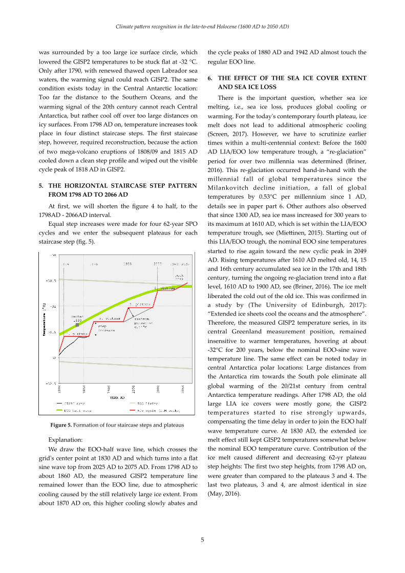
5. THE HORIZONTAL STAIRCASE STEP PATTERN FROM 1798 AD TO 2066 AD

At first, we will shorten the figure 4 to half, to the 1798AD - 2066AD interval.

Equal step increases were made for four 62-year SPO cycles and we enter the subsequent plateaus for each staircase step (fig. 5).

Explanation: We draw the EOO-half wave line, which crosses the

grid's center point at 1830 AD and which turns into a flat sine wave top from 2025 AD to 2075 AD. From 1798 AD to about 1860 AD, the measured GISP2 temperature line remained lower than the EOO line, due to atmospheric cooling caused by the still relatively large ice extent. From about 1870 AD on, this higher cooling slowly abates and

the cycle peaks of 1880 AD and 1942 AD almost touch the regular EOO line.

6. THE EFFECT OF THE SEA ICE COVER EXTENT AND SEA ICE LOSS

There is the important question, whether sea ice melting, i.e., sea ice loss, produces global cooling or warming. For the today's contemporary fourth plateau, ice melt does not lead to additional atmospheric cooling (Screen, 2017). However, we have to scrutinize earlier times within a multi-centennial context: Before the 1600 AD LIA/EOO low temperature trough, a “re-glaciation” period for over two millennia was determined (Briner, 2016). This re-glaciation occurred hand-in-hand with the millennial fall of global temperatures since the Milankovitch decline initiation, a fall of global temperatures by 0.53°C per millennium since 1 AD, details see in paper part 6. Other authors also observed that since 1300 AD, sea ice mass increased for 300 years to its maximum at 1610 AD, which is set within the LIA/EOO temperature trough, see (MieKinen, 2015). Starting out of this LIA/EOO trough, the nominal EOO sine temperatures started to rise again toward the new cyclic peak in 2049 AD. Rising temperatures after 1610 AD melted old, 14, 15 and 16th century accumulated sea ice in the 17th and 18th century, turning the ongoing re-glaciation trend into a flat level, 1610 AD to 1900 AD, see (Briner, 2016). The ice melt liberated the cold out of the old ice. This was confirmed in a study by (The University of Edinburgh, 2017): “Extended ice sheets cool the oceans and the atmosphere”. Therefore, the measured GISP2 temperature series, in its central Greenland measurement position, remained insensitive to warmer temperatures, hovering at about -32°C for 200 years, below the nominal EOO-sine wave temperature line. The same effect can be noted today in central Antarctica polar locations: Large distances from the Antarctica rim towards the South pole eliminate all global warming of the 20/21st century from central Antarctica temperature readings. After 1798 AD, the old large LIA ice covers were mostly gone, the GISP2 temperatures started to rise strongly upwards, compensating the time delay in order to join the EOO half wave temperature curve. At 1830 AD, the extended ice melt effect still kept GISP2 temperatures somewhat below the nominal EOO temperature curve. Contribution of the ice melt caused different and decreasing 62-yr plateau step heights: The first two step heights, from 1798 AD on, were greater than compared to the plateaus 3 and 4. The last two plateaus, 3 and 4, are almost identical in size (May, 2016).

�5

Figure 5. Formation of four staircase steps and plateaus


7. ADJUSTMENT OF THE STAIRCASE-PLATEAU PATTERN

As the staircase paKern is the result of a harmonic solar SPO movement, the paKern needs to be adjusted into a sine wave. This wave-like temperature change was observed as “expanded stadium wave” (WyaK and Curry, 2013) as demonstrated in the paper Annex (fig. A3). We can also observe this wave in the GISSTEMP temperature graph (see Annex, fig. A4). The final temperature evolution graph is as shown in figure 6.

Observations: From 1818 AD to 2066 AD (peak to peak) or 1798 AD to 2046 AD (plateau end to plateau end), we observe four cycles, 62 years in length, varying in their amplitude of about 0.16°C on the GISP2 borehole scale.

Concerning the 30th EOO cycle, the peak date is the year 2049 AD. From there on, the 31st period will commence with 446 years of declining temperatures. Present temperatures, since 2004 AD, as the 62-year cycle peak, will continue as plateau, which should even decline by 0.1-0.2°C until the plateau end in 2046 AD. Figures of present ocean temperatures, both, in the Atlantic and the Pacific, demonstrate this ongoing SST temperature plateau, see two AMO and PDO graphs in the Annex (figs A5 and A6). The most recent data on ocean cooling is the heat content graph for the North Atlantic, showing Atlantic water cooling 2006-2017 AD by NOCD data. The 62-yr wave like cooling proceeds as well in the Southern Hemisphere, see figure 4, for 2000-2017 AD, on the Antarctic Peninsula in (Oliva, 2017), as well in the eastern and central tropical Pacific (Bordbar, 2016). The land-

based temperatures, however, will stay somewhat above plateau level, due to “innovative” temperature readings, which homogenize temperature series upwards.

Another method for raising land temperatures is the UHI-effect, which yields an up to +4°C temperature increase in UHI locations (Benz, 2017). Another method is the “airporterization” of measurement locations, drawing on the asphalt runway heat.

However, the continuing temperature plateau over the next two and half decades will soon demonstrate that most warming models and simulations are without scientific merit.

7. SUMMARY AND CONCLUSIONS ON THE HOLOCENE PATTERN RECOGNITION ANALYSIS

The Climate PaKern Recognition analysis is the only available analysis, which places the time span 1600 AD to 2050 AD within a multi-millennial Holocene context, in which five identified climate forcing mechanisms visibly act for more than 10,000 years. The discussed time span from 1600 AD onwards started with the coldest LIA temperature boKom trough, as a beginning of the 30th cycle, from where on temperatures moved upward, demanded both by the half-wave cycle and the 62-year SPO cycle, to rise to our present warm CWP with its top in 2049 AD.

We enumerate major achievements from our paper parts 1-8: Identification of the growing EOO cycle from its beginning in 8108 BC (paper part 1), identification of cosmic meteor impacts on Earth, which always produce a double, one cold, followed by a warm temperature spike (papers part 1 to 7), identification of two Taurids Stream periods (paper part 3 and 5), identification of the Milankovitch temperature decline initiation towards the next glacial (paper part 6), identification of EMB (Earth-Moon-Barycenter) stabilization process (paper part 7), identification of the 62-year SPO cycle (paper part 7), identification of causes for the temperature increase since the LIA until today, causes for the continuation of the present temperature plateau and for the 2049 AD top temperature peak (paper part 8). This top temperature peak was previously calculated in a theoretical, physical-astronomical study in 2010 AD (Seifert, J. 2010), which we substantiated with 10,000 years of empirical Holocene evidence. All in all, five cosmic forcing mechanisms are the true causes of the Holocene temperature evolution. Each of the five climate forcing mechanisms was demonstrated in this series and each individual temperature spike and peak, which occurred within the entire Holocene was analyzed. One should also mention, that, on the other hand, a large assortment of GCM models and simulations exist, all of which have failed

�6

Figure 6. SPO wave temperature increase 1798 - 2066 AD


model-observation comparisons. Only the PaKern Recognition analysis is capable to explain each single temperature peak of the Holocene. The underperformance of other models and simulations can easily be explained. Fundamental causes are: 1. Their omission of decadal and centennial cosmic Earth orbital variations, and 2. The omission of solar motion variations. Instead, models and simulations exclusively center on internal atmosphere-ocean system variables, combined to some extremely long Milankovitch features, 20 - 40 kyr in length, with which centennial and single millennium features cannot be explained. Therefore, underperformance must be the logical result (ScafeKa, 2013). We emphasize again, that the present fourth flat temperature plateau, since 2004 AD, will continue until 2046 AD, the end of the recent 62-year SPO cycle.

REFERENCES

Alley, R.B.: The Younger Dryas cold interval as viewed from central Greenland, Quaternary Science Reviews, Volume 19, Issues 1-5, 2000, hKp://www.ncdc.noaa.gov/paleo/icecore/greenland/greenland.html,

Alley, R.B. : GISP2 Ice Core Temperature and Accumulation Data. IGBP Pages/World Data Center for Paleoclimatology, Data ContributionSeries #2004-013, NOAA/NGDC Paleoclimatology Programs, Boulder, CO, USA

Benz, S.A. et.al.: Identifying anthropogenic anomalies in air, surface and groundwater temperatures in Germany, Science of The Total Environment, vol. 584-585, Apr 2017, p.145-153

hKps://doi.org/10.1016/j.scitotenv.2017.01.139 Bordbar, M.H.; et.al.: Role of Internal Variability in Recent

Decadal to Multidecadal Tropical Pacific Climate C h a n g e s , G e o p h y s . R e s . L e K . , 4 4 , d o i : 1 0 . 1 0 0 2 / 2 0 1 6 G L 0 7 2 3 5 5 , h K p : / / d x . d o i . o r g /10.1002/2016GL072355

Briner, J.P. et. al.: Holocene climate change in Arctic Canada and Greenland, Quaternary Science Reviews, vol. 147, Sep 2016, p. 340-364 hKp://doi.org/10.1016j.quascirev.2016.02.010 Blog: hKp://www.climate4you with actualized North Atlantic heat content data

Ljungqvist, F.C., 2010: A new reconstruction of temperature variability in the extra-tropical Northern Hemisphere during the last two millennia, Geogr. Ann., 92A (3), p.339-351

DeLong, K.L.; Quinn, T.M. et.al.: Sea surface temperature variability in the southwest Pacific since 1649, nature climate change, vol.2, p.799-804, Nov 2012 doi: 10.1038/nclimate1583

May, Andy: Virtually indistinguishable — comparing early 20th century warming to late 20th century warming, in: hKp://www.WUWT, 22. August 2016

Medhang, I. et.al.: Reconciling controversies about the `global warming hiatus`, Nature, no. 42, vol. 545, May 2017, doi: 10.1038/nature 22315

MieKinen, A.; et.al.:Exceptional ocean surface conditions on the SE Greenland Shelf during the Medieval Climate Anomaly, Paleoceanography, vol. 30, issue 12, p. 1657-1674, Dec 2015, doi: 10.1002/2015PA002849

Moberg, A., et.al.: Highly variable Northern Hemisphere temperatures reconstructed from low- and high-resolution proxy data, Nature, vol. 433, no.7026, pp. 613-617, Feb 2005, doi: 10.1038/nature 03265

Murphy, L.N., et. al.: The role of historical forcings in simulating the observed Atlantic multidecadal oscillation, Geophys. Res. LeK., vol 44, nr. 5, p.2472-2480, Mar 2017, doi: 10.1002/2016GL071337

Oliva, M. et.al.: Recent regional climate cooling on the Antarctic Peninsula and associated impacts on the cryosphere, Science of the Total Environment, vol 580, 15 Feb 2017, p. 210-223, hKps://doi.org/10.1016/j.scitotenv.2016.12.030

ScafeKa, N.: Solar and Planetary Oscillation Control on Climate Change: Hindcast, Forecast and a Comparison with CMIP5 GCMs, Energy and Environment, 24, no. 3&4, 2013, doi: 10.1260/0958-305X.24.3-4.455 hKp://www.duke.edu/~ns2002/pdf/scafeKa_EE_2013.pdf

Screen, J.A.: The missing Northern European winter cooling response to Arctic sea ice loss, Nature Communications 8, article no. 14603 (2017) doi: 10.1038/Incomms 14603

Seifert, J.: Das Ende der globalen Erwärmung, Berechnung des Klimawandels, (2010), 109 pp., Pro Business Verlag B e r l i n , I S B N 9 7 8 - 3 - 8 6 8 0 5 - 6 0 4 - 4 , h K p : / /www.amazon.de/Das-Ende-globalen-Erwärmung-Klimawandels/dp/3868056041

Sigl, M.; Winstrup, M. et.al.: Timing and climate forcing of volcanic eruptions for the past 2,500 years, Nature 523, 543-549 (30 July 2015) doi: 10.1038/nature 14565

Stenni, B. et.al: Antarctic climate variability at regional and continental scales over the last 2,000 years, Clim.Past.Discuss., doi: 10.5194/cp-2017-40, 2017

Stocker, T.F.; Mysak, L.A.: Climatic fluctuations of the century time scale: A review of high-resolution proxy data and possible mechanisms, Climate Change, 20, p. 227-250, March 1992, Kluver Academic Publishers, NL, hKp:/ /www.cl imate.unibe.ch/~stocker/papers/stocker92cc.pdf

�7


Tejedor, E.; et.al.: Temperature variability in the Iberian Range since 1602 inferred from tree ring records, Clim. Past, 13, 93-105, 2017 doi: 10.5194/cp-13-93-2017 hKp: / /www.Antarct ic_s tudy_sheds_l ight_on-central_ice_sheet/The_University_of-Edinburgh

Wikipedia: Famine, hKps://en.wikipedia.org/wiki/Famine, last accessed October 2017

WyaK and Curry: Expanded stadium wave, hKps://judithcurry.com/2013/10/10/the-stadium-wave

�8


Annex

�9

Figure A1. EOO-LIA boKom trough (MieKinen, 2015)

Figure A2. Temperature variability in the Iberian Range since 1602 inferred from tree ring records (Tejedor, 2017)


�10

Figure A3. Expanded stadium wave (WyaK and Curry, 2013)

Figure A4. Observed station based temperatures (GISS) and harmonic solar SPO movement.


�11

Figure A6. Pacific Decadal Oscillation along with the 62-year SPO pulsation cycle.

Figure A5. Atlantic Multidecadal Oscillation index computed as the linearly detrended North Atlantic sea surface temperature anomalies 1856-2013 along with the 62-year SPO pulsation cycle.

Documents

CLIMATE PATTERN RECOGNITION IN THE LATE-TO … · CLIMATE PATTERN RECOGNITION IN THE LATE-TO-END ... half-wave cycle commenced in 8108 BC, ... 1. INTRODUCTION This 500 year period