Embed Size (px)
Citation preview
Climate Sensitivity of Groundwater Systems Critical for Agricultural Incomes in South India
R. Balasubramanian
Working Paper No. 96–15
Published by the South Asian Network for Development and Environmental Economics (SANDEE)PO Box 8975, EPC 1056, Kathmandu, Nepal.Tel: 977-1-5003222 Fax: 977-1-5003299
SANDEE research reports are the output of research projects supported by the SouthAsian Network for Development and Environmental Economics. The reports have beenpeer reviewed and edited. A summary of the findings of SANDEE reports are alsoavailable as SANDEE Policy Briefs.
National Library of Nepal Catalogue Service:
R. BalasubramanianClimate Sensitivity of Groundwater Systems Critical for Agricultural Incomes in South India
(SANDEE Working Papers, ISSN 1893-1891; WP 96–15)
ISBN: 978-9937-596-25-1
Key words: Climate change Groundwater table Farm income Spatial dynamic panel data Tamil Nadu.
SANDEE Working Paper No. 96–15
Climate Sensitivity of Groundwater Systems Critical for Agricultural Incomes in South India
R. BalasubramanianProfessor of Agricultural EconomicsTamil Nadu Agricultural UniversityCoimbatore-641 003
June 2015
South Asian Network for Development and Environmental Economics (SANDEE) PO Box 8975, EPC 1056, Kathmandu, Nepal
SANDEE Working Paper No. 96–15
The South Asian Network for Development and Environmental Economics
The South Asian Network for Development and Environmental Economics (SANDEE) is a regional network that brings together analysts from different countries in South Asia to address environment-development problems. SANDEE’s activities include research support, training, and information dissemination. Please see www.sandeeonline.org for further information about SANDEE.
SANDEE is financially supported by the International Development Research Center (IDRC), The Swedish International Development Cooperation Agency (SIDA), the World Bank and the Norwegian Agency for Development Cooperation (NORAD). The opinions expressed in this paper are the author’s and do not necessarily represent those of SANDEE’s donors.
The Working Paper series is based on research funded by SANDEE and supported with technical assistance from network members, SANDEE staff and advisors.
AdvisorCeline Nauges
Technical EditorMani Nepal English EditorCarmen Wickramagamage
Comments should be sent to
R. BalasubramanianProfessor of Agricultural Economics, Tamil Nadu Agricultural University, Coimbatore-641 003Email: [email protected]
Contents
Abstract1. Introduction 1
2. Climate Change and Groundwater Irrigation 2
2.1 Impact of Climate Variables on Groundwater Dynamics 2 2.2 Climate Change Impact on Irrigated Agriculture 2
3. Study Area and Data 4
3.1 Description of Study Site 4 3.2 Data Sources 5
4. Modeling the Impact of Climate Change on Groundwater Irrigated Agriculture 6
4.1 Measuring Climate Sensitivity of Groundwater Aquifers – Spatial Dynamic Panel Data Approach 6 4.2 Impact of Groundwater Level and Climatic Variables on Farm Income 6 4.3 Empirical Model 7 4.4 Estimation Strategy 7
5. Results and Discussion 8
5.1 Impact of Climate Change on Groundwater Dynamics 8 5.2 Climate Change, Groundwater Dynamics and Farm Income 9
6. Conclusions and Policy Implications 10
Acknowledgements 11
References 12
Tables
Table 1: Definition of Variables and Their Descriptive Statistics 16Table 2: Regression Estimates of Factors Affecting Depth to Water Table (in meters) 16Table 3: Regression Estimates of Factors Affecting Net Returns per ha (INR/ha) 17Table 4: Estimated Elasticity Values for Net Returns Equation 18
Figures
Figure 1: Spatial Variability in Water Level and Climate Variables 19Figure 2: Temporal Variability in Water Level and Climate Variables 19
South Asian Network for Development and Environmental Economics6
AbstractThere are few economic studies that have estimated the impact of climate variables on agriculture by identifying their impacts on irrigation sources, even though irrigation serves as a critical adaptation strategy for farmers’ in water-deficit countries such as India. In this study, we examine the implications of variations in climate variables on ground water sources of irrigation and agricultural income in the Indian state of Tamil Nadu. Our findings, based on a panel of 11 districts observed over a 40-year period, suggest that while increases in rainfall positively influence the water table, increases in maximum temperature significantly reduce ground water availability. There is also significant spatial correlation in water levels across districts. In terms of impacts on farm income, groundwater availability and free electricity have a positive effect, while increases in well density have a negative effect on income. Significantly, temperature has an inverted U-shaped relationship with income, with income decreasing at temperatures higher than a threshold temperature of 34.31°C. In our panel dataset, this threshold temperature has already been breached 61 times or in 14 % of the total number of observations. As temperatures increase as a result of climate change, our findings raise two important practical concerns for agricultural management: a) ground water reductions are likely and alternate sources of irrigation may need to be identified; and, b) because richer farmers are able to dig deeper wells, electricity subsidies will benefit the rich more and small land holders are likely to
see lower returns to agriculture with increases in well density.
Key words
Climate change, groundwater table, farm income, spatial dynamic panel data, Tamil Nadu.
1
Climate Sensitivity of Groundwater Systems Critical for Agricultural Incomes in South India
Climate Sensitivity of Groundwater Systems Critical for Agricultural Incomes in South India
1. Introduction
Groundwater is the source of approximately one third of global water withdrawals and provides drinking water for a large portion of the global population. In many regions, it is subject to stress with respect to both quantity and quality (Kundzewicz and Döll, 2009). Climate change will have serious consequences for groundwater recharge and thus for renewable groundwater resources (Konikow and Kendy, 2005; Döll, 2009; Haddeland et al., 2013). Ficklin et al. (2010) for instance, have found elevated CO2 concentration in the atmosphere and changes in temperature to have a significant effect on groundwater recharge. India is the largest groundwater user in the world with an estimated annual groundwater withdrawal of 270 km3 out of which more than one-fourth (68 km3) is contributed by nonrenewable groundwater resources (Wada et al., 2012). More than 60 percent of India’s irrigated acreage is dependent on groundwater and a high 85 percent of rural India’s drinking water requirement is met from groundwater. Shah (2009) argues that western and peninsular India are groundwater hotspots from a climate change point of view. In many parts of India, particularly in the hardrock and coastal aquifers of South India, groundwater overexploitation and saline ingress from seawater are common.
In addition to its impact on groundwater recharge, climate change will also increase the use of groundwater. If the availability of surface water shrinks, groundwater use usually increases. Where groundwater is already the dominant water resource, the amount of water used could increase due to higher demands as a result of high evaporation rates. In India, 50 percent of water used for irrigation comes from groundwater. Increases in extraction with reductions in recharge will contribute to groundwater resources depleting relatively quickly (Ludwig and Moench, 2009). Therefore, Loáiciga (2003) emphasizes the need to adapt aquifer exploitation to suit climate variability and climate change. In spite of the intricate interrelationship between climate variables and groundwater and the growing significance of groundwater in sustaining agricultural productivity, systematic studies of the impact of climate and non-climate variables on groundwater balance and agricultural production are scarce (Alley, 2001; Bates et al., 2008). In the Indian context, such studies are almost non-existent. Our study is an attempt to fill this lacuna through a systematic analysis of the climate-groundwater-agriculture nexus.
Climate change impacts will add to existing pressure on groundwater resources: (i) directly through changes in groundwater recharge or supply; and (ii) indirectly through changes in demand for groundwater (Taylor et al., 2012). While climate change impacts on groundwater supplies through changes in recharge, its impact on demand is more complex. In general, climate change will result in an increase in water demand due to increase in evapotranspiration (caused by higher temperature and lower rainfall). Ground water demand will also increase to offset reduced surface water availability, and due to climate-induced changes in crop patterns. Thus, understanding the impact of climate variability and change on the availability and sustainability of surface water and groundwater resources is of tremendous ecological and economic value (Dragoni and Sukhija, 2008).
This paper seeks to: i) to examine the relationship between climate variables and groundwater dynamics; and ii) to analyze the implications of climate change for groundwater availability and farm income in order to identify suitable measures for adaptation to climate change. It addresses the impact of climate change on groundwater supply and its consequences for irrigated agriculture by analyzing panel data, covering a period of 40 years from 1971 to 2010, from the South Indian state of Tamil Nadu.
The study findings, based on spatial econometric analysis, suggest that current and one-period lagged rainfall have a significant effect in reducing the depth to water table, while the area under water-intensive crops and maximum temperature increase the depth to water table. Depth to water level is defined as the vertical distance measured
South Asian Network for Development and Environmental Economics2
from the ground level (well head) to the actual depth at which water is available in the well. Thus, increases in rainfall and maximum temperature, as expected, increase and decrease ground water availability. There is also significant spatial correlation in water level across districts. This implies that groundwater levels across districts are correlated due to overlapping of aquifers across district boundaries. Temperature shows an inverted U-shaped relationship with farm income. In the panel dataset comprising 440 observations, this threshold temperature of 34.31°C has already been breached 61 times or in about 14 per cent of observations Depth to water table, i.e., ground water availability, has a significant positive impact on farm income. Thus, in the future, as temperature increases managing climatic changes and groundwater availability will be critical for farm income.
2. Climate Change and Groundwater Irrigation
2.1 Impact of Climate Variables on Groundwater DynamicsAs a dynamic natural resource, groundwater is subject to a high degree of variability across time and space. Climate change affects the hydrological cycle and has an uncertain impact on groundwater resources, with climatic factors, viz., rainfall and temperature, likely to be highly correlated with groundwater availability and use. As Okkonen et al. (2010) have shown, global warming is expected to cause lower water tables and decreased groundwater discharge while the extraction of groundwater is likely to increase to meet the growing demand for water. Climate variability has a direct bearing on crop production through its impact on the physiology of crop growth and soil moisture availability while it indirectly affects agriculture through its impact on surface water availability and groundwater recharge. Future climate change, together with other drivers of change, is likely to intensify current agricultural water management challenges in Africa and India (Brown and Hansen, 2008). Therefore, a systematic investigation of the impact of climate and non-climate factors on recharge and withdrawal of groundwater and the possible risks posed to groundwater resources under different climate-change scenarios is of paramount importance.
Two broad approaches have been used in the literature to study the impact of climate change on groundwater resources. The first is the physical approach wherein the changes in groundwater reserves are quantified by physical measurements using hydrological modeling such as the water balance method or GIS and simulation modeling. The second is the empirical or statistical modeling approach where the changes in groundwater levels are estimated statistically through building a statistical relationship between groundwater level and rainfall, temperature, and other variables.
Many researchers have also used regression analysis incorporating climate- and/or non-climate variables to study the impact of these variables on water table levels (Ferguson and George, 2003; Ngongondo, 2006; Balasubramanian, 1998; and Balasubramanian and Swaminathan, 2000). Using the regression analysis of groundwater levels with monthly rainfall data, Bloomfield et al. (2003) predicted groundwater levels under different future climates in the United Kingdom. This study revealed that even with a small increase in the total annual rainfall, the annual groundwater level could fall in the future due to changes in seasonality and increased frequency of drought events. In their study of the Texas Edwards Aquifer of USA, Chen et al. (2001) used a log-log regression model to study the impact of climate variables, viz., temperature and rainfall, on groundwater levels. They found that changes in climatic conditions reduce water resource availability and increase water demand leading to a substantial welfare loss to the regional economy.
2.2 Climate Change Impact on Irrigated AgricultureThe climate change impact on agriculture through groundwater irrigation assumes significance in predominantly groundwater-irrigated areas because both changes in temperature and precipitation will affect irrigation availability and demand. Reduction in precipitation is likely to further intensify aquifer exploitation for agriculture and place additional burdens on other surface and groundwater resources for non-agricultural use (Kurukulasuriya and Rosenthal, 2003). There are two distinct but inter-related issues concerning the treatment of irrigation in economic studies on the impact of climate change on agriculture: a) the issue of the climate-sensitivity of irrigated vs. rain-fed farms, which entails carrying out separate or pooled analyses of the climate change impact on irrigated and rainfed farms; and b) the inclusion of irrigation as one of the explanatory variables in the regression model. The
3
Climate Sensitivity of Groundwater Systems Critical for Agricultural Incomes in South India
early Ricardian models did not account for irrigation in analyzing the climate change impact and ignored the afore-mentioned issues. One of the problems in including irrigation in the climate change impact models is that it is an endogenous choice by farmers which in turn is sensitive to climate change (Mendelsohnet al., 1994). Since both the supply and demand for irrigation water are affected by climate change, the inclusion of irrigation as an explanatory variable is important though problematic. Further, as several studies have pointed out, exclusion of irrigation is inappropriate due to the fact that irrigation is one of the important adaptation strategies to circumvent the hotter and drier climatic conditions. In response to a criticism by Darwin (1999) of the original Ricardian model by Mendelsohn et al. (1994) Mendelsohn and Nordhaus (1999) included irrigation as one of the explanatory variables in their model by addressing the problem of the climate-endogeneity of irrigation. Towards this end, Kurukulasuriya et al, (2011) developed a structural Ricardian model in which irrigation adoption is modeled as an endogenous choice, and the predicted choice/frequency of irrigation is then included as an additional independent variable in the final model of climate change impact.
Irrigation was explicitly incorporated into the econometric model in a pioneering study by Mendelsohn and Dinar (2003). In this study, self-reported farmland values were regressed on climate, soil, economic, demographic and irrigation variables. The study, which also included climate interaction terms with water and irrigation variables, found that while surface irrigation has a small effect on the climate sensitivity of agriculture, groundwater withdrawals are not significant because they are endogenous in the model. The study points to the need for adapting to climate change through irrigation and adoption of water-saving technologies.
The proposition that irrigation is an important adaptation mechanism for climate change gained further strength after Schlenker et al. (2005) argued that irrigation breaks the link between the growth of a plant and the climate. Since then, most subsequent studies have used irrigation as one explanatory variable. Farm-level impact studies provide adequate opportunities to model irrigation both as an endogenous adoption decision as well as an exogenous variable affecting farm land values (Kurukulasuriya and Mendelsohn, 2008; Mendelsohn and Dinar, 2003). Many studies have treated irrigation as an exogenous variable in econometric models of climate change impact assessment. For example, Polsky (2004) estimated Ricardian regression equations for six different time points in US agriculture and found that groundwater irrigation from the Ogallala aquifer has a significant effect on farm land values buffering the impact of climate sensitivities while similar results were also reported from Africa (Gbetibouo and Hassan, 2005). Similarly, another study found that access to irrigation water (water quota) has a positive impact on farm profits in Israel. As water quotas are allocated by the Israel Water Commissioner, the study treated the water quota as exogenous to the farmers. In addition to the positive impact of irrigation on farm profits, the inclusion of the irrigation variable in the model affected the estimated climate coefficients. Hence, econometric models that omit irrigation water in regions with irrigation will tend to over-predict the global warming impacts (Fleischer et al., 2008).
In the conventional Ricardian models of climate change, farmland value or its proxy, viz., farm profits, is regressed on climate normals (i.e., the long-term average of climate variables for a particular cross-sectional unit) with a cross section of samples drawn from regions/locations showing sufficient variation in their climatic conditions. Deschênes and Greenstone (2007) proposed an alternative to this approach by using random, year-to-year variability in weather parameters such as precipitation and temperature on farm profits. Consequently, this approach allows the use of panel data to estimate the effect of weather on farm profits, conditional on locations by year fixed effects. Kavikumar (2011) too followed this approach in his analysis of 271 Indian districts over a period of 20 years to estimate the impact of climate change on farm net revenue. Baylis et al. (2011) extended the panel data approach suggested by Deschênes and Greenstone (2007) by incorporating spatial effects into the model to study the climate change impact on US agriculture.
Studies that have explicitly incorporated groundwater availability and/or withdrawal in climate change impact models in agriculture are, however, very limited. Among the few studies that have incorporated groundwater irrigation in economic models of climate change impacts on agriculture, none has studied the twin effects of the climate change impact on groundwater and its impact on agricultural productivity and/or farm income via groundwater. For example, Schlenker et al. (2007) examined the impact of climate variables, surface water availability and depth to groundwater on farmland values in California using the Ricardian analysis. Their analysis shows that while surface water availability had a significant positive impact on farmland values, they did not find
South Asian Network for Development and Environmental Economics4
depth to groundwater table to have a statistically significant impact. Though a study by Chen et al. (2001) estimated both the climate change impact on groundwater and its subsequent impact on the regional economy including agriculture, it has used mathematical programming and simulation modeling rather than econometric models to quantify economic impacts.
3. Study Area and Data
3.1 Description of Study SiteThis study was carried out in the state of Tamil Nadu in South India where groundwater aquifers are under severe stress due to poor groundwater management caused by a lack of groundwater regulatory institutions and perverse incentives such as fully subsidized electricity for groundwater pumping (World Bank, 2010). More than 70 percent of the Tamil Nadu state is underlain by low-storage aquifers that are heavily exploited (Foster and Garduño, 2004). As the surface water resource potential in the state is already fully exploited, groundwater assumes enormous significance in the state. Consequently, groundwater irrigation in the state has expanded rapidly in the last five decades due to the decline and/or instability in surface irrigation sources, massive expansion in rural electrification, the advent of modern well-drilling technologies, and the subsidized supply of electricity for groundwater pumping. According to CGWB (2008) in more than one-third of blocks1in Tamil Nadu, groundwater is overexploited. The key policy challenges in the sustainable management of groundwater resources in Tamil Nadu revolve around energy pricing for groundwater pumping, watershed development programs to enhance groundwater recharge, increasing water use efficiency through drip and sprinkler technologies, investments in stabilizing surface water sources in order to reduce the pressure on groundwater, and regulation of well drilling. Hence, this study addresses the critical challenges posed by climate change for groundwater resources and its consequences for irrigated agriculture for the purpose of identifying appropriate policy and institutional mechanisms to ensure sustainable groundwater management in Tamil Nadu.
The state of Tamil Nadu is located in the southern-most part of India and is divided into seven agro-climatic regions that display wide diversity in climate and crops cultivated. The average annual rainfall varies from 30.51 cm to 210.70 cm in the plains with a mean of 96.92 cm and a standard deviation of 34.49. The mean annual maximum temperature varies from 30.53 to 35.26 degrees Celsius with a mean of 33.03°C and a standard deviation of 1.07. Even though the state benefits from both the north-east and south-west monsoons, the south-west monsoon accounts for only about 30 percent of the total annual rainfall while the north-east monsoon accounts for about 50 percent with summer rains contributing 15 percent and the winter rains the rest. The main sources of irrigation in the state of Tamil Nadu are wells, canals originating from large reservoirs or river systems, and tanks2. Most of the canal systems in the state are dependent on rivers originating from outside the state of Tamil Nadu and hence are very much influenced by rainfall occurring outside the state. Canal irrigation is predominantly prevalent in the central districts with water-intensive crops such as rice and sugarcane as the main crops and tank irrigation predominant in the coastal plains. Wells are the main source of irrigation, on the other hand, in the northern, western, and north-western districts. The canal and tank systems are characterized by the cultivation of a few water-intensive crops such as rice, sugarcane, banana, and turmeric while well irrigation is characterized by a wide array of crops such as coconut, maize, sugarcane, cotton, groundnut, fruits, and vegetables. Both irrigation intensity and cropping intensity3 in the state have been showing a declining trend. The cropping intensity has declined from about 120 percent in 1960 to 113 percent in 2010 while the irrigation intensity has decreased from more than 130 percent to 113 percent during the same period.
In spite of the substantial role played by surface irrigation sources, viz., canals and tanks, the dependence on groundwater has been increasing steadily over time as the water availability from the surface sources is highly volatile and uncertain. While the total area irrigated from surface irrigation sources, viz., tanks and canals, has
1 Blocks are the lowest administrative units in the State at which groundwater recharge and pumping volumes are estimated.2 Tanks are fairly large, man-made, earthen embankments constructed across a valley or slope to impound and store rainfall run-off that use the water thus stored for irrigation.3 Cropping intensity refers to the percentage of gross cropped area to net cropped area. Irrigation intensity is defined as the percentage of gross irrigated area by all sources to net irrigated area by all sources. The gross cropped area is the sum total of net cropped area and area cropped more than once during a year.
5
Climate Sensitivity of Groundwater Systems Critical for Agricultural Incomes in South India
decreased considerably from more than 1.80 million ha in the 1960-61 to about 1.30 million ha in 2010, the total number of groundwater wells has increased from about 0.87 million to 1.90 million and the area irrigated by wells has increased from 0.6 million ha to 1.6 million ha over the last fifty years. The growth in groundwater irrigation is the result of considerable policy and institutional support in the form of liberal institutional credit for well-drilling, subsidized pricing of electricity for groundwater pumping, and the absence or non-implementation of regulatory mechanisms for mitigating groundwater overexploitation. Over the last forty years, electricity pricing for agricultural pumping has undergone significant changes from a pro-rata tariff in the 1970s and early 1980s, to a system of flat-tariff in the late 1980s, to, finally, a fully subsidized electricity supply for agriculture from 1990-91 onwards. The introduction of the “zero-marginal-cost” pricing of electricity (after the introduction of the flat-rate tariff) along with the advent of modern, low-cost well-drilling technologies, has provided added impetus to the drilling of deep bore-wells in many parts of the state during the last two decades. Private investments in the deepening of existing wells and the drilling of new bore-wells have also continued unabated. By and large, it could therefore be argued that the regimen of groundwater governance in the state has gone into disarray which has contributed to the unfettered increase in both the number and depth of wells. This places the state of Tamil Nadu as one of the groundwater hotspots in India, thus making it an ideal location to study the impact of climate change on groundwater resources.
3.2 Data SourcesWe collected time-series data on depth to water level from 1740 observation wells4 spread over the entire state of Tamil Nadu, and the corresponding data on rainfall, temperature, number of groundwater wells and surface water sources, and the area of various crops cultivated with groundwater and surface water irrigation, from government publications. Spatial distribution of observation wells across the entire state with different endowments of surface water resources, aquifer formations and related hydro-geological and socio-economic factors was helpful in dividing the entire state into several cross-sectional units. We compressed the water-level data for individual wells into district-level averages which helped us to conduct the panel data analysis of groundwater table fluctuations vis-à-vis climatic- and non-climatic variables, with districts serving as cross-sectional units. During the period of 40 years from 1971 to 2010, for which the water-level data are available, electricity pricing for groundwater pumping, institutional arrangements for groundwater management, availability and performance of other sources of irrigation, viz., canals and tanks, and the technology for well-drilling have undergone significant changes. Therefore, these factors provide sufficient scope and rationale to systematically estimate the impact of climate change on groundwater irrigation in Tamil Nadu. This will, in turn, provide interesting insights into the complex interrelationship between natural, anthropogenic, and institutional factors, on the one hand, and groundwater irrigated agriculture on the other.
The second part of the analysis, which is concerned with the impact of climatic factors along with groundwater level changes on agricultural crop production, relies on agricultural crop production data at district level to estimate net revenue per ha from crop production. We sourced the data on crop-wise, district-level average productivity (yield in kg/ha) from Season and Crops Reports for Tamil Nadu, published by the Government of Tamil Nadu for the entire study period from 1971 to 2010. We assembled the matching data on costs of cultivation from the Government of India Scheme on Cost of Cultivation of Principal Crops that is being implemented in the Department of Agricultural Economics, Tamil Nadu Agricultural University. Using these two sets of data on input quantities, yield, and input and output prices, we constructed data on the average net income per ha for 11 districts of Tamil Nadu for 40 years (1971 to 2010). We included the predominantly groundwater-irrigated crops, viz., rice, maize, banana, coconut, cotton, sugarcane, sesame, groundnut, tapioca and turmeric, in the estimation of net returns. After estimating the net returns per ha for each crop using the district-level average yield and cost of cultivation data described above, we worked out the weighted average net returns per ha. As the area under different crops vary widely across districts and over time, we have computed the weighted average net income per ha from these crops using as weights the share of the area under kth crop to total cropped area under all these crops in ith district in year t. We computed the weighted average input and output prices using the data on deflated prices of agricultural outputs and inputs. In constructing the weighted average of input prices, we used the share of individual inputs to total cost
4 Observation wells refer to the wells that are used as samples for taking water-level measurements. Water level measurements are taken every month. Depth to water level is defined as the vertical distance measured from the ground level (well head) to the actual depth at which water is available in the well.
South Asian Network for Development and Environmental Economics6
of cultivation of each of the individual crops as weights while using the share of individual crop area to total cropped area in each district as weights in calculating the weighted average of output price.
4. Modeling the Impact of Climate Change on Groundwater Irrigated Agriculture
4.1 Measuring Climate Sensitivity of Groundwater Aquifers – Spatial Dynamic Panel Data Approach
Climate change impacts agriculture directly through the impact of temperature and rainfall on crop growth, and indirectly through the changes in the supply of and demand for groundwater irrigation. This paper adopts a two-step modeling approach to quantify both of these effects. In the first step, we quantified the impact of climate variables on groundwater aquifers (depth to water table) while, in the second stage, we estimated the impacts of climate variables and groundwater levels on farm income. As a dynamic natural resource, the current level of groundwater aquifers, which is determined by the initial stock and natural recharge, and the extraction for various uses, are characterized by both temporal and spatial externalities. Hence, quantifying the climate change impact on groundwater levels is a complicated exercise demanding knowledge of both the hydrology of aquifers and the economics of water extraction and use. The availability of long-period panel data on the groundwater level and climate variables permits the estimation of the dynamic consequences of rainfall, temperature and previous-period water levels on current-period water levels. As our dataset on all climate, non-climate, and groundwater variables is assembled at district level, the possible non-coincidence of aquifer boundaries with district boundaries poses problems in precisely estimating the aquifer response to climate variables5. To address this problem, we introduce a spatial lag in the dependent variable (water level) so that any influence of water level in a district on the neighboring districts due to the overlapping of aquifers is accounted for by the spatial lag of the dependent variable. The presence of both the time- and spatial-lag of the dependent variable necessitates the use of the spatial dynamic panel data model to estimate the climate sensitivity of groundwater levels.
Spatial panel data models have gained in importance in recent times6. Researchers divide them into two broad categories, viz., spatial static panel models and spatial dynamic panel data models. The spatial dynamic panel model is an extension of the static spatial panel model in that it includes the time-lagged dependent variable as one of the explanatory variables. To estimate spatial dynamic panel data models, econometricians use both maximum likelihood estimation (MLE) and generalized method of moments (GMM) estimators. GMM is the preferred choice where there is a problem of endogeneity in explanatory variables. However, in spatial econometrics, the GMM estimator is less accurate than the ML estimator due to the unbounded estimation by GMM (Yang, 2009). Elhorst (2003) has developed unconditional maximum likelihood estimators for spatial dynamic panel data. Further, Elhorst (2008) who compared Spatial MLE, Spatial Dynamic MLE and difference-GMM, found that the spatial dynamic MLE had better overall performance in terms of reduced bias and low RMSE. In situations where the assumption of the MLE method is not likely to hold, the Quasi-Maximum Likelihood estimation (QMLE) is used. Yu et al.(2008) and Lee and Yu (2010) have demonstrated the asymptotic properties and applications of the QML estimator for spatial dynamic panel data models while Monteiro (2010) has observed that the spatial dynamic quasi-maximum likelihood estimator is the best among the spatial estimators in terms of the RMSE criterion and that it is more robust. Further, QMLE can be consistent even when the disturbances are not normally distributed (Lee, 2004).
4.2 Impact of Groundwater Level and Climatic Variables on Farm IncomeGroundwater availability is an indicator of agrarian prosperity in much of the hardrock regions in India. Access to groundwater provides insurance against stochastic surface water supplies and the vagaries of monsoon rains.
5 There are four major aquifers in the State of Tamil Nadu, viz., Alluvium (17.50 percent of area) Charnockite (25.65 percent) Gneiss (37.22 percent) and Banded Gneissic Complex (7.86 percent) each covering more than one district with the other minor types covering only a very small area (CGWB, 2012). Therefore, there is potential spatial interdependence across districts in terms of depth to water table.6 Spatial panel models are used in fields as wide as agricultural economics (Druska and Horrace, 2004; Gutierrez and Sassi, 2012) climate change impact on agriculture (Baylis et al., 2011; Kavikumar, 2011) regional growth convergence (Baltagi et al., 2007; Ertur and Koch, 2007) public economics (Zheng et al., 2013) labor economics (Foote, 2007) economics of consumption and habit formation (Korniotis, 2010) and the effect of financial reforms among countries (Elhorst, 2013). Barring Druska and Horrace (2004) and Baylis et al. (2011) all other studies mentioned above used spatial dynamic panel data models.
7
Climate Sensitivity of Groundwater Systems Critical for Agricultural Incomes in South India
Groundwater thus is both a productive and protective input besides affecting the use of other inputs. Further, the depth to the water table is an important determinant of both the fixed and variable costs of groundwater pumping as it affects the depth of the well as well as the variable cost of energy used in lifting water. In this paper, we have used the annual mean depth to water table7 as the dependent variable in the first equation of the econometric model. Besides determining the cost of pumping, the water table level serves as a signal to the farmers about the quantity of the water available so as to enable them to decide about the crop pattern, thus becoming an important determinant of profits from groundwater agriculture. Hence, the second part of this paper is concerned with the estimation of the net returns equation incorporating the estimated depth to water table as one of the explanatory variables. In what follows, we elaborate on the empirical model and estimation strategy.
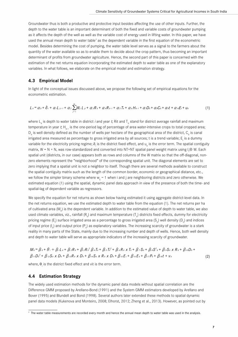
4.3 Empirical ModelIn light of the conceptual issues discussed above, we propose the following set of empirical equations for the econometric estimation.
where Lit is depth to water table in district i and year t; Rit and Tit stand for district average rainfall and maximum temperature in year t; Hit-1 is the one-period lag of percentage of area water-intensive crops to total cropped area; Dit is well density defined as the number of wells per hectare of the geographical area of the district, Cit is canal irrigated area measured as percentage to gross irrigated area by all sources; t is a trend variable; Et is a dummy variable for the electricity pricing regime; δi is the district fixed effect, and uit is the error term. The spatial contiguity matrix, W = N × N, was row-standardized and converted into NT×NT spatial panel weight matrix using IT⊗ W. Each spatial unit (districts, in our case) appears both as rows and columns of the W matrix so that the off-diagonal, non-zero elements represent the “neighborhood” of the corresponding spatial unit. The diagonal elements are set to zero implying that a spatial unit is not a neighbor to itself. Though there are several methods available to construct the spatial contiguity matrix such as the length of the common border, economic or geographical distance, etc., we follow the simpler binary scheme where wij = 1 when i and j are neighboring districts and zero otherwise. We estimated equation (1) using the spatial, dynamic panel data approach in view of the presence of both the time- and spatial-lag of dependent variable as regressors.
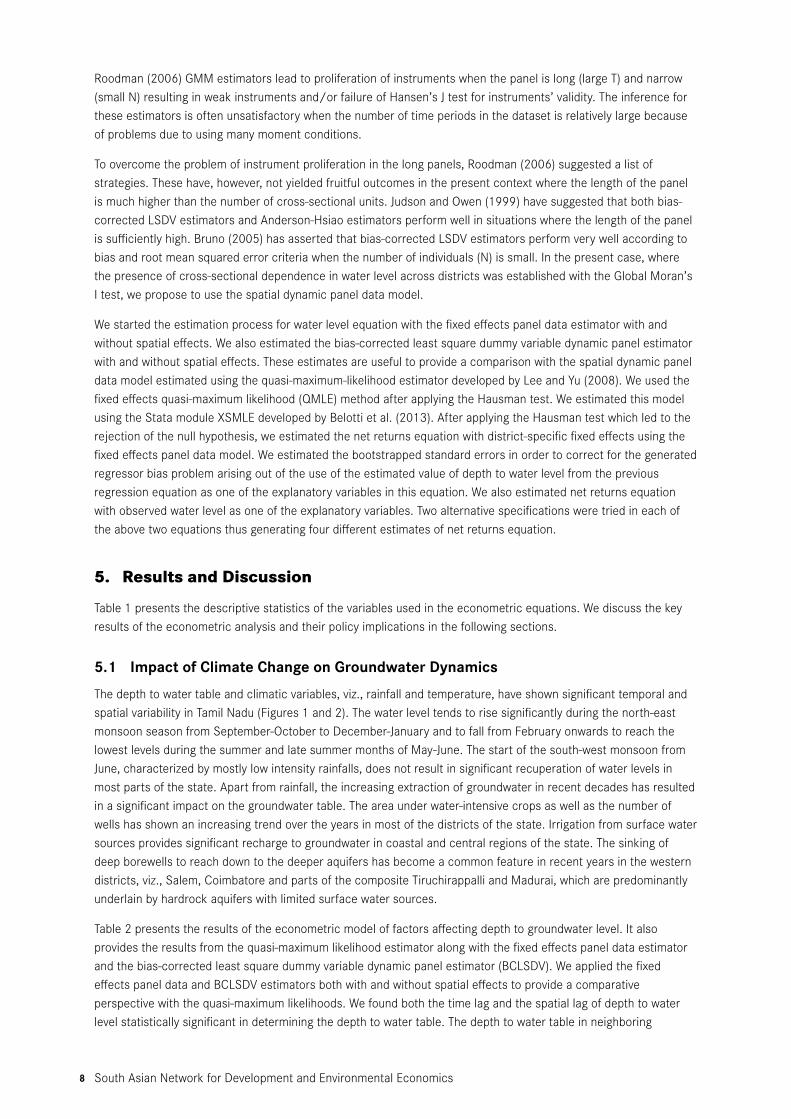
We specify the equation for net returns as shown below having estimated it using aggregate district-level data. In the net returns equation, we use the estimated depth to water table from the equation (1). The net returns per ha of cultivated area (Mit) is the dependent variable. In addition to the estimated value of depth to water table, we also used climate variables, viz., rainfall (Rit) and maximum temperature (Tit) districts fixed effects, dummy for electricity pricing regime (Et) surface irrigated area as a percentage to gross irrigated area (Sit) well density (Dit) and indices of input price (Iit) and output price (Pit) as explanatory variables. The increasing scarcity of groundwater is a stark reality in many parts of the State, mainly due to the increasing number and depth of wells. Hence, both well density and depth to water table will serve as appropriate indicators of the increasing scarcity of groundwater.
where, qi is the district fixed effect and vit is the error term.
4.4 Estimation StrategyThe widely used estimation methods for the dynamic panel data models without spatial correlation are the Difference GMM proposed by Arellano-Bond (1991) and the System GMM estimators developed by Arellano and Bover (1995) and Blundell and Bond (1998). Several authors later extended these methods to spatial dynamic panel data models (Kukenova and Monteiro, 2008; Elhorst, 2012; Zheng et al., 2013). However, as pointed out by
7 The water table measurements are recorded every month and hence the annual mean depth to water table was used in the analysis.
L it = a0 + d i + a1L i,t–1 + a2 Wijj= 1
N
/ L jt + a3R it + a4R it–1 + a5 Tit + a6 Hit–1 + a7Dit + a8Cit + a9t + a10Et + uit (1)
Mit = b 0 + i i + b1L it + b 2R it + b 2R it2 b 4Tit + b 5 Tit
2 + b 6 R it x Tit + b 7 Sit + b 8S2it + b 9Sit x R it + b10Dit +
b11Dit2 + b12Sit x Dit + b13R it x Dit + b14Sit x R it x Dit + b15 E t + b16 E it + b17 Pit + b18t + v it (2)
South Asian Network for Development and Environmental Economics8
Roodman (2006) GMM estimators lead to proliferation of instruments when the panel is long (large T) and narrow (small N) resulting in weak instruments and/or failure of Hansen’s J test for instruments’ validity. The inference for these estimators is often unsatisfactory when the number of time periods in the dataset is relatively large because of problems due to using many moment conditions.
To overcome the problem of instrument proliferation in the long panels, Roodman (2006) suggested a list of strategies. These have, however, not yielded fruitful outcomes in the present context where the length of the panel is much higher than the number of cross-sectional units. Judson and Owen (1999) have suggested that both bias-corrected LSDV estimators and Anderson-Hsiao estimators perform well in situations where the length of the panel is sufficiently high. Bruno (2005) has asserted that bias-corrected LSDV estimators perform very well according to bias and root mean squared error criteria when the number of individuals (N) is small. In the present case, where the presence of cross-sectional dependence in water level across districts was established with the Global Moran’s I test, we propose to use the spatial dynamic panel data model.
We started the estimation process for water level equation with the fixed effects panel data estimator with and without spatial effects. We also estimated the bias-corrected least square dummy variable dynamic panel estimator with and without spatial effects. These estimates are useful to provide a comparison with the spatial dynamic panel data model estimated using the quasi-maximum-likelihood estimator developed by Lee and Yu (2008). We used the fixed effects quasi-maximum likelihood (QMLE) method after applying the Hausman test. We estimated this model using the Stata module XSMLE developed by Belotti et al. (2013). After applying the Hausman test which led to the rejection of the null hypothesis, we estimated the net returns equation with district-specific fixed effects using the fixed effects panel data model. We estimated the bootstrapped standard errors in order to correct for the generated regressor bias problem arising out of the use of the estimated value of depth to water level from the previous regression equation as one of the explanatory variables in this equation. We also estimated net returns equation with observed water level as one of the explanatory variables. Two alternative specifications were tried in each of the above two equations thus generating four different estimates of net returns equation.
5. Results and Discussion
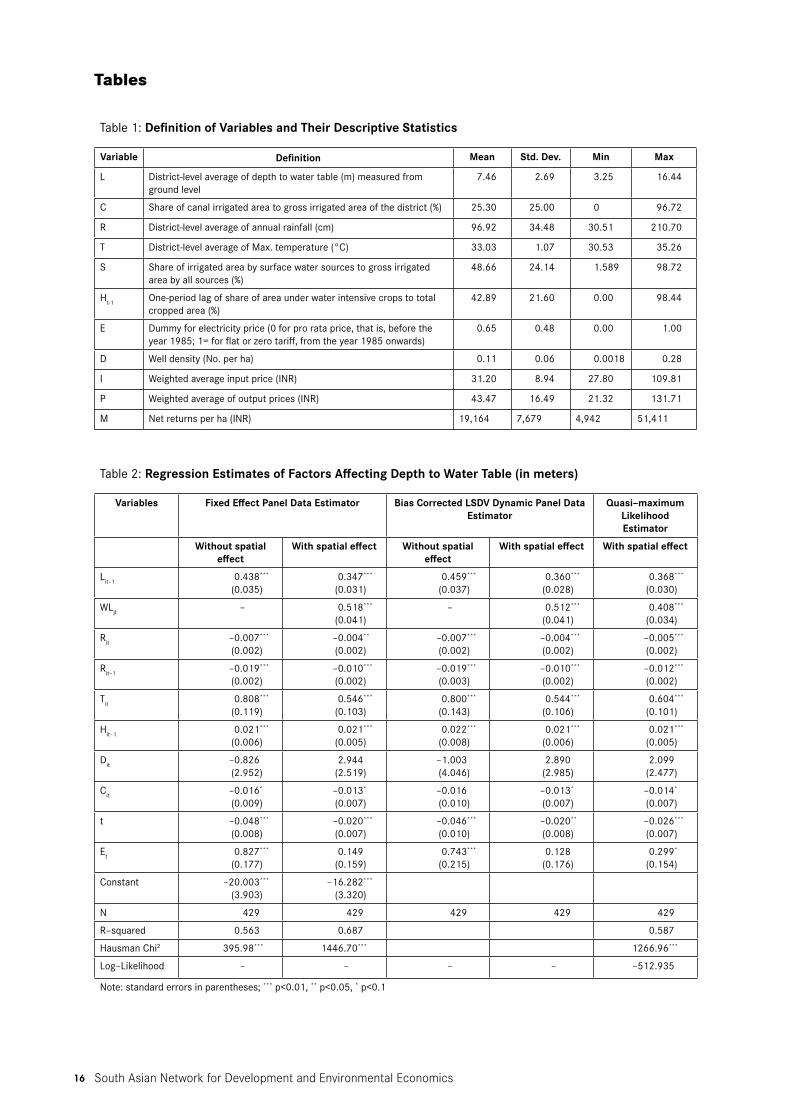
Table 1 presents the descriptive statistics of the variables used in the econometric equations. We discuss the key results of the econometric analysis and their policy implications in the following sections.
5.1 Impact of Climate Change on Groundwater DynamicsThe depth to water table and climatic variables, viz., rainfall and temperature, have shown significant temporal and spatial variability in Tamil Nadu (Figures 1 and 2). The water level tends to rise significantly during the north-east monsoon season from September-October to December-January and to fall from February onwards to reach the lowest levels during the summer and late summer months of May-June. The start of the south-west monsoon from June, characterized by mostly low intensity rainfalls, does not result in significant recuperation of water levels in most parts of the state. Apart from rainfall, the increasing extraction of groundwater in recent decades has resulted in a significant impact on the groundwater table. The area under water-intensive crops as well as the number of wells has shown an increasing trend over the years in most of the districts of the state. Irrigation from surface water sources provides significant recharge to groundwater in coastal and central regions of the state. The sinking of deep borewells to reach down to the deeper aquifers has become a common feature in recent years in the western districts, viz., Salem, Coimbatore and parts of the composite Tiruchirappalli and Madurai, which are predominantly underlain by hardrock aquifers with limited surface water sources.
Table 2 presents the results of the econometric model of factors affecting depth to groundwater level. It also provides the results from the quasi-maximum likelihood estimator along with the fixed effects panel data estimator and the bias-corrected least square dummy variable dynamic panel estimator (BCLSDV). We applied the fixed effects panel data and BCLSDV estimators both with and without spatial effects to provide a comparative perspective with the quasi-maximum likelihoods. We found both the time lag and the spatial lag of depth to water level statistically significant in determining the depth to water table. The depth to water table in neighboring
9
Climate Sensitivity of Groundwater Systems Critical for Agricultural Incomes in South India
districts appears to have a significant impact on the depth to water table in a district as indicated by the regression coefficient of the spatial lag of the dependent variable. We found the climatic variables, viz., both current period and one-period lagged rainfall, as well as maximum temperature to be statistically significant in impacting the groundwater table. This showed the marginal impact of one period lagged rainfall to be more than twice that of the current period rainfall. We expect that an additional rainfall of 100 cm during the current period would reduce the depth to water table by about 0.5 meters while a similar increase in the previous year rainfall is likely to reduce the depth to water table by more than one meter.
As expected, the maximum temperature had a significant impact on increasing the depth to groundwater table which is the direct result of increased evapotranspiration which in turn would lead to a lower recharge as well as higher withdrawal of groundwater to compensate for evapotranspiration. An increase in the current period temperature by one degree Celsius will increase the depth to water table by about 0.60 meters, which requires more than 100 cm of current period rainfall to offset. Hence, any increase in future temperature is likely to have very serious consequences for groundwater resources by increasing groundwater demand and reducing recharge. Similarly, cultivation of water-intensive crops has a strong deleterious effect on the depth to water table. A 1 percent increase in the share of area under water-intensive crops would increase the depth to water table by 0.02 meters. Hence, a steady increase in the area under water-intensive crops poses challenges to the sustainability of scarce groundwater reserves. Canal irrigation has a positive role in improving the water table. A 1 percent increase in the share of area under canal irrigation reduced the depth to water table by about 0.014 meters. However, the negative role of water-intensive crops could only be partially offset by canal irrigation. This result seems plausible given the fact that the area under water-intensive crops such as coconut has been increasing steadily even in non-canal irrigated areas where groundwater is the mainstay of agriculture. The dummy variable for electricity pricing has turned out to be statistically significant with a positive sign indicating that the subsidy for electricity has led to an increase in the depth to water table, probably due to over-pumping. The trend variable, which would probably capture various time-varying factors like private and public investments in water-harvesting (watershed programs) and water-saving (drip irrigation) structures, had a significant impact in reducing the depth to water table. The overall explanatory power of the spatial dynamic panel data model with an R-squared value of 0.59 indicates that the model is a good fit for the data.
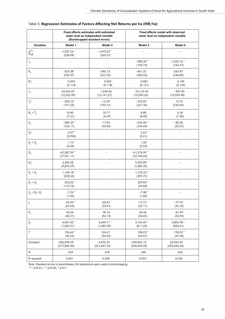
5.2 Climate Change, Groundwater Dynamics and Farm IncomeThe second part of the econometric exercise is concerned with the estimation of the net returns equation in which we used the estimated value of the depth to water table from the previous section of the econometric analysis (QML estimation) as the explanatory variable along with other exogenous variables. Table 3 presents the results of the fixed effects panel data regression with bootstrapped standard errors while Table 4 presents the estimated elasticities (at the sample mean).
Results presented in Table 3 pertain to four alternative specifications of net returns equation for the purpose of comparison. The models with estimated and observed depth to water table are almost similar in most of the coefficients, with estimated water table depth producing a larger marginal effect on net returns than observed water table depth. We use model 1 for the purposes of interpretation and drawing conclusions. The estimated water level turned out to be statistically significant at 1 percent level. An increase in depth to the water table by one meter will reduce the net farm income by about INR 1550 per ha (USD 26, at the prevailing exchange rate of USD 1=INR 60) which is about 8 percent of the mean net returns in our sample. Alternatively, a 1 percent increase in depth to water table above the mean level will lead to 0.61 percent reduction in net income.
Maximum temperature and its quadratic term are statistically significant with the expected signs indicating the inverted U-shaped relationship between maximum temperature and net returns. The net income reaches its maximum value at 34.31°C and starts decreasing thereafter. In our dataset comprising 440 observations shows that temperatures have been higher than this threshold level 61 times or in 14% of observations. However, in terms of elasticity at the mean level, a 1 percent increase in temperature beyond the mean temperature of 33.03°C will result in an increase in net returns by about 1.64 percent. But this mean temperature is very close to the threshold value, after which returns will decline.
South Asian Network for Development and Environmental Economics10
An increase in the share of surface irrigated area by 1 percent would lead to a reduction in net income by about 0.13 percent. The share of area under surface irrigation appears to have a U-shaped relationship indicating that an increase in surface irrigated area, to start with, has a negative effect probably due to the uncertainties associated with the surface system. However, beyond the threshold of 57.20 percent, the percentage share of surface irrigated area turns out to have a positive effect on net revenue by facilitating intensive cropping and the raising of commercial, high-value crops such as turmeric, banana and sugarcane. This is further corroborated by the significance of the two interaction terms—the percentage share of surface irrigated area with rainfall and well density. The positive effect of these two interaction terms indicates that an increase in rainfall or surface irrigation availability would increase both the quantity and certainty of overall water availability for agriculture through enhanced aquifer recharge or the conjunctive use of surface and groundwater sources. This is also evident from the first-stage regression where we found canal irrigation to play a positive role in increasing the water level.
We also found well density to have a negative impact on net returns, with its elasticity value indicating that a 1 percent increase in well density above the mean level would lead to a reduction in net returns by about 0.13 percent. Even though well density per se had a negative effect on farm incomes, the positive interaction effect of rainfall with well density and with surface irrigation provides scope for increasing groundwater irrigation under conditions of good rainfall and in areas with surface water potential. As both rainfall and surface water contribute towards groundwater recharge and groundwater irrigation in turn contributes towards mitigating the uncertainties associated with rainfall and surface water supply, this result appears to be plausible. This also lends credence to the argument that irrigation wells could be a means of enhancing farm productivity and income where there is sufficient recharge from rainfall or surface water bodies. Conversely, groundwater wells could be a means of enhancing the quantum and certainty of water supply for agricultural irrigation.
The dummy variable for the electricity pricing regime, which has changed from pro rata pricing to zero-marginal cost pricing (with the introduction of flat-rate pricing in 1984-85 and the subsequent 100 percent subsidy for irrigation pumping) indicates that the shift to the zero-marginal cost pricing regime has increased net farm income by more than INR 4,000 per ha (USD 67 per ha) on average. A comparison of the regression coefficients for the depth to water table and the electricity pricing dummy reveals that the positive effect of the electricity subsidy on farm income is more than twice the negative effect of the falling water table on farm income. This is probably because zero-marginal cost pricing encourages farmers to extract water from deeper aquifers and cultivate high water-intensive commercial crops resulting in higher farm incomes. Perhaps this is the economic logic behind individual farmers’ continuous attempts to extract water alongside the increasing social costs of depleting groundwater and the financial burden of the subsidy. Leaving aside significant social costs, the electricity subsidy has also aggravated the unequal access to groundwater irrigation. However, the strong political lobby in favor of a full subsidy for electricity for agriculture due to the positive—albeit in the short run—private benefits of the electricity subsidy continues to hold sway in the debates on electricity pricing for agricultural water pumping. While the output price index was not statistically significant, the input price index was found to be significant at the 5 percent level. An increase in input prices by 1 percent will result in a loss of net returns by 0.15 percent. The regression coefficient of the trend (time) variable which could be expected to capture technological progress over time has turned out to be positive and statistically significant indicating that net returns at constant prices have increased over time, probably due to technological progress in agriculture.
6. Conclusions and Policy Implications
The absence to date of a systematic assessment of the direct impact of climate variables on farm income as well as their indirect impact on farm income through groundwater supply and demand is an important gap in the existing literature. Our study, based in the South Indian state of Tamil Nadu, where groundwater resources are under severe stress, addresses this gap.
Econometric analysis of groundwater availability reveals that climate variables, viz., increases in current and one-period lagged rainfall, increase groundwater availability, while increases in maximum temperature and the share of area under water-intensive crops reduce groundwater availability. There are significant spatial effects in the groundwater availability across districts. There is a strong positive relationship between water availability and farm
11
Climate Sensitivity of Groundwater Systems Critical for Agricultural Incomes in South India
income because of the dependence of farmers on this source of irrigation. The analyses also show that temperature affects agricultural incomes both directly and indirectly through its impact on groundwater availability. Temperature has an inverted U-shaped relationship with farm income. Beyond a threshold temperature being 34.31°C, farm incomes fall. Our panel dataset with 440 observations shows that temperatures have been higher than this threshold level 61 times. This finding points to the need for adaptation strategies that temperature proof agriculture through reduced evapotranspiration strategies and effective water conveyance and application mechanisms.
An important policy implication of the analysis is the negative impact of well density and the positive effect of the electricity subsidy on farm income. The sinking of new wells, especially deep bore wells, needs to be regulated. Though free electricity has a positive impact on average farm net revenues, this comes at a social cost. Large farmers with financial resources are likely to continue drilling deeper wells, while small and marginal farmers may be the ones most likely to suffer from the negative externalities of higher well density. In this scenario, an electricity subsidy will mainly benefit large land-holding farmers (Balasubramanian, 1998; Howes and Murgai, 2003; Jain, 2006). The possibility of a partial or full rollback of the electricity subsidy and the regulation of well density puts both the policy makers and the farmers in a tight spot in the current political climate. This is because the short-term interests of both farmers (especially the large-farmer lobby) and politicians would be better-served if the subsidies continue. One policy option to prioritize is pro-rata electricity pricing and/or volumetric restriction on pumping in exchange for increased public investments and/or subsidies for recharge programs and water conservation investments. Innovative approaches that combine a mix of institutional interventions such as well-spacing and deep well permits (Howe, 2002) and market-based instruments such as electricity pricing (Shah et al., 2008) could play a role.
The shift to water-intensive crops such as coconut and sugarcane in response to increasing labor scarcity is another factor contributing to increased groundwater extraction, with serious distributional implications. Our study, based on average net revenues at the district level, cannot throw light on who gains and who loses from groundwater over-exploitation -- further analysis is required to understand the distributional implications of the cultivation of water-intensive crops. Since farmers strongly respond to market signals in deciding crop choice and patterns, regulatory mechanisms may not be very effective. Appropriate incentive structures such as subsidies for water-saving crops and/or technologies could be alternative mechanisms. Public and private investments in groundwater recharge such as watershed development, percolation ponds, recharge wells and farm ponds are additional considerations.
Acknowledgements
The author wishes to thank the South Asian Network for Development and Environmental Economics (SANDEE) for the generous financial support to carry out this research. He would also like to record his appreciation of the team of SANDEE advisors comprising Jean-Marie Baland, Enamul Haque, Céline Nauges, Subhrendu Pattanayak, E. Somanathan and Jeffrey Vincent as well as his fellow SANDEE researchers who offered valuable comments and suggestions at the Research and Training Workshops held in Colombo, Kathmandu and Bangkok during 2011-2013. The author wishes to extend a special thanks to his advisor Céline Nauges for her assiduous guidance and incisive comments at various stages of the study. Priya Shyamsundar, Executive Director, SANDEE, has been a great source of inspiration, support and guidance for the last one and a half decades, for which the author is ever grateful to her. The author feels very much indebted to his diligent SANDEE friends, Pranab Mukhopadhyay and Mani Nepal, who made his stint with SANDEE a memorable learning experience. Thanks are also due to Anuradha Kafle and Neesha Pradhan, the secretarial staff of SANDEE, who kept me on track with various communications and reporting deadlines.
South Asian Network for Development and Environmental Economics12
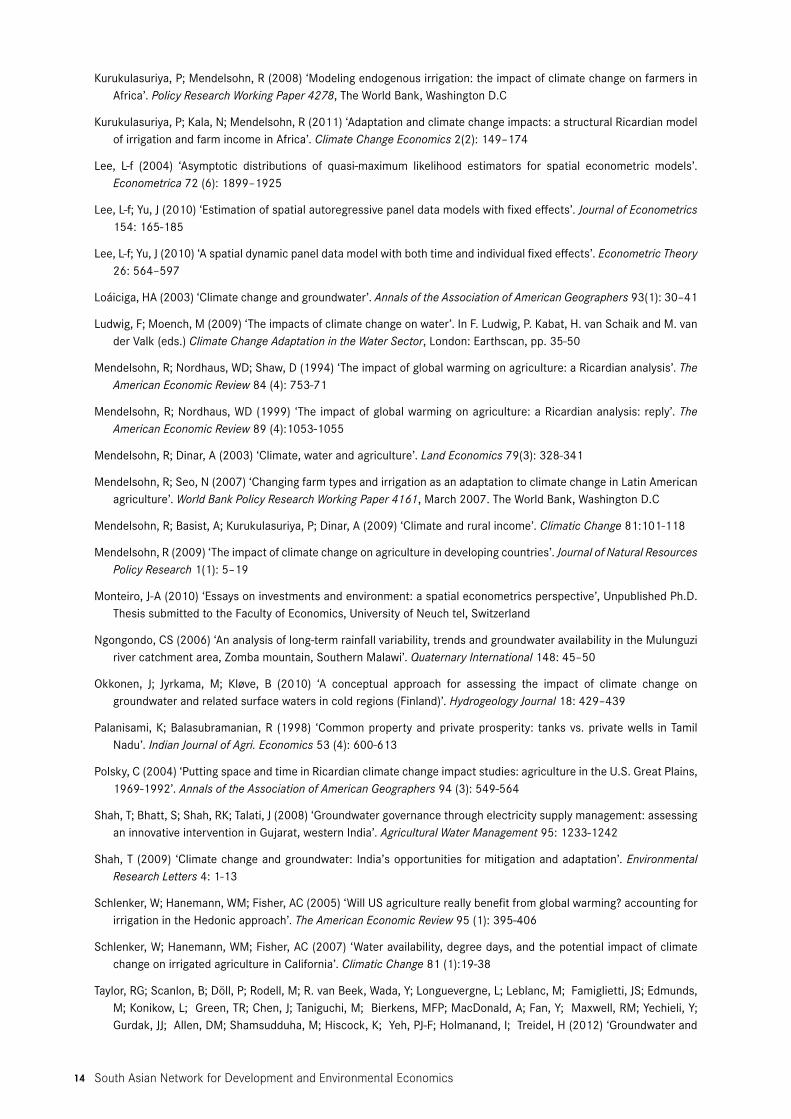
References
Alley, WM (2001) ‘Ground water and climate’. Ground Water 39(2):161
Arellano, M; Bond, SR (1991) ‘Some tests of specification for panel data: Monte Carlo evidence and an application to employment equations’. Review of Economic Studies 58: 277-297
Balasubramanian, R (1998) ‘An enquiry into the nature, causes and consequences of growth of well irrigation in a vanguard agrarian economy’, PhD Thesis submitted to the Department of Agricultural Economics, Tamil Nadu Agricultural University, Coimbatore, India
Balasubramanian, R; Swaminathan, LP (2000) ‘Groundwater overexploitation in hardrock regions: economic analysis of causes and consequences’. In Choudhury, RC; Singh, RP (eds) Rural Prosperity and Agriculture: Policies and Strategies, Hyderabad: National Institute of Rural Development, pp. 68-103
Balasubramanian, R (2008) ‘Community tanks vs private wells: coping strategies and sustainability issues in South India’. In Ghate, R; Jodha, NS; Mukhopadhyay, P (eds) Promise, Trust and Evolution: Managing the Commons of South Asia, Oxford: Oxford University Press, pp.283-304
Baltagi, B; Bresson, G; Pirotte, A (2007) ‘Panel unit root tests and spatial dependence’. Journal of Applied Econometrics 22: 339–360
Bates, BC; Kundzewicz, ZW; Wu, S; Palutikof, JP (2008) ‘Climate change and water’. Technical Paper VI of the Intergovernmental Panel on Climate Change, Geneva: IPCC Secretariat, 210 pp
Baylis, K; Paulson, ND; Piras, G (2011) ‘Spatial approaches to panel data in agricultural economics: a climate change application’. Journal of Agricultural and Applied Economics 43(3): 325-338
Belotti, F; Hughes, G; Mortari, AP (2013) ‘XSMLE: Stata module for spatial panel data models estimation’, Statistical Software Components S457610, Department of Economics, Boston College, Boston
Bloomfield, JP; Gaus, I; Wade, SD (2003) ‘A method for investigating the potential impacts of climate-change scenarios on annual minimum groundwater levels’. Water and Environment Journal 17 (2): 86-91
Brown, C; Hansen, JW (2008) ‘Agricultural water management and climate risk’, Report to the Bill and Melinda Gates Foundation. IRI Tech. Rep. No. 08-01. International Research Institute for Climate and Society, New York, 19 pp
Bruno, GSF (2005) ‘Estimation and inference in dynamic unbalanced panel data models with a small number of individuals’. Working Paper WP 165, Centro di Ricerca sui Processi di Innovazione e Internazionalizzazione, Milano
CGWB (Central Groundwater Board) (2012) ‘Aquifer systems of Tamil Nadu and Puducherrry’, Southern Regional Office, Ministry of Water Resources, Government of India, Chennai
Chen, C; Gillig, D; McCarl, BA (2001) ‘Effects of climate change on a water dependent regional economy: a study of the Texas Edwards Aquifer’. Climate Change 49: 397-409
Darwin, R (1999) ‘The impact of global warming on agriculture: a Ricardian analysis: comment’. American Economic Review 89 (4):1049-52
Deschênes, O; Greenstone, M (2007) ‘The economic impacts of climate change: evidence from agricultural output and random fluctuations in weather’. American Economic Review 97 (1): 354-385
Döll, P (2009) ‘Vulnerability to the impact of climate change on renewable groundwater resources: a global-scale assessment’. Environment Research Letters 4: 1-12.
Dragoni, W; Sukhija, BS (2008) ‘Climate change and groundwater - a short review’, In W. Dragoni and B. S. Sikhija (eds.) Climate Change and Groundwater, London: Geological Society, Special Publications, v. 288, pp. 1–12
Druska, V; Horrace, WC (2004) ‘Generalized moments estimation for spatial panel data: Indonesian rice farming’. American Journal of Agricultural Economics 86 (1): 185-198
Ertur, C; Koch, W (2007) ‘Growth, technological interdependence and spatial externalities: theory and evidence’. Journal of Applied Econometrics 22: 1033–1062
Elhorst, JP (2003) ‘Specification and estimation of spatial panel data models’. International Regional Science Review 26 (3): 244–68
13
Climate Sensitivity of Groundwater Systems Critical for Agricultural Incomes in South India
Elhorst, JP (2008) ‘Estimation of dynamic panels with endogenous interaction effects’, Paper presented at the Second World Conference of the Spatial Econometrics Association, 17-19, November, 2008, New York Marriot, New York, USA
Elhorst, P (2012) ‘Dynamic spatial panels: models, methods, and inferences’. Journal of Geographical Systems 14: 5–28
Elhorst, P; Zandberg, E; Haan, JD (2013) ‘The impact of interaction effects among neighboring countries on financial liberalization and reform: a dynamic spatial panel data approach’. Spatial Economic Analysis 8 (3): 293-313
Ferguson, G; Scott St. George (2003) ‘Historical and estimated ground water levels near Winnipeg, Canada, and their sensitivity to climatic variability’. Journal of the American Water Resources Association 39 (5): 1249-1259
Ficklin, D; Luedeling, E; Zhan, M (2010) ‘Sensitivity of groundwater recharge under irrigated agriculture to changes in climate, CO2 concentrations and canopy structure’. Agricultural Water Management 97 (7): 1039-1050
Fleischer, A; Lichtman, I; Mendelsohn, R (2008) ‘Climate change, irrigation, and Israeli agriculture: will warming be harmful?’ Ecological Economics 65 (3): 508-515
Foote, CL (2007) ‘Space and time in macroeconomic panel data: young workers and state-level unemployment revisited’. Working Paper No. 07-10, Federal Reserve Bank of Boston, Boston
Foster, S; Garduño, H (2004) ‘India - Tamil Nadu: resolving the conflict over rural groundwater use between drinking water & irrigation supply’. Case Profile Collection Number 11, Sustainable Groundwater Management Lessons from Practice, Global Water Partnership Associate Program, The World Bank, Washington D.C
Gutierrez, L; Sassi, M (2012) ‘Spatial and non-spatial approaches to agricultural convergence in Europe’. Economia and Diritto Agroalimentare 17: 9-38
Gbetibouo, GA; Hassan, RM (2005) ‘Measuring the economic impact of climate change on major South African field crops: a Ricardian approach’. Global and Planetary Change 47: 143–152
Haddeland, I; Heinke, J; Biemans, H; Eisner, S; Flörke, M; Hanasaki, N; Konzmann, M; Ludwig, F; Masaki, Y; Schewe, J; Stacke, T; Tessler, ZD; Wada, Y; Wisser, D (2013) ‘Global water resources affected by human interventions and climate change’. Proceedings of the National Academy of Sciences 111(9): 3251-3256. doi: 10.1073/pnas.1222475110 (accessed on February 21, 2014)
Howe, C (2002) ‘Policy issues and institutional impediments in the management of groundwater: lessons from case studies’. Environment and Development Economics 7: 625–641. Available at: DOI:10.1017/S1355770X02000384
Howes, S; Murgai, R (2003) ‘Incidence of agricultural power subsidies: an estimate’. Economic and Political Weekly 38 (16): 1533-35
Jain, V (2006) ‘Political economy of electricity subsidy: evidence from Punjab’. Economic and Political Weekly 41 (38): 4072-80
Judson, RA; Owen, AL (1999) ‘Estimating dynamic panel data models: a guide for macroeconomists’. Economics Letters 65: 9–15
Kavikumar, KS (2011) ‘Climate sensitivity of Indian agriculture: do spatial effects matter?’ Cambridge Journal of Regions, Economy and Society 4: 221–235
Konikow, L; Kendy, E (2005) ‘Groundwater depletion: a global problem’. Hydrogeology 13 (1): 317-320
Korniotis, GM (2010) ‘Estimating panel models with internal and external habit formation’. Journal of Business and Economic Statistics 28(1): 145-158
Kukenova, M; Monteiro, J-A (2008) ‘Spatial dynamic panel model and system GMM: a Monte Carlo investigation’, IRENE Working Papers 09–01, Irene Institute of Economic Research, University of Neuchâtel, Neuchâtel, Switzerland
Kundzewicz, ZW; Döll, P (2009) ‘Will groundwater ease freshwater stress under climate change?’ Hydrol. Sci. J. 54 (4): 665–675
Kurukulasuriya, P; Rosenthal, S (2003) ‘Climate change and agriculture: a review of impacts and adaptations’. Climate Change Series Paper No.91, The World Bank, Washington D.C
South Asian Network for Development and Environmental Economics14
Kurukulasuriya, P; Mendelsohn, R (2008) ‘Modeling endogenous irrigation: the impact of climate change on farmers in Africa’. Policy Research Working Paper 4278, The World Bank, Washington D.C
Kurukulasuriya, P; Kala, N; Mendelsohn, R (2011) ‘Adaptation and climate change impacts: a structural Ricardian model of irrigation and farm income in Africa’. Climate Change Economics 2(2): 149–174
Lee, L-f (2004) ‘Asymptotic distributions of quasi-maximum likelihood estimators for spatial econometric models’. Econometrica 72 (6): 1899–1925
Lee, L-f; Yu, J (2010) ‘Estimation of spatial autoregressive panel data models with fixed effects’. Journal of Econometrics 154: 165-185
Lee, L-f; Yu, J (2010) ‘A spatial dynamic panel data model with both time and individual fixed effects’. Econometric Theory 26: 564–597
Loáiciga, HA (2003) ‘Climate change and groundwater’. Annals of the Association of American Geographers 93(1): 30–41
Ludwig, F; Moench, M (2009) ‘The impacts of climate change on water’. In F. Ludwig, P. Kabat, H. van Schaik and M. van der Valk (eds.) Climate Change Adaptation in the Water Sector, London: Earthscan, pp. 35-50
Mendelsohn, R; Nordhaus, WD; Shaw, D (1994) ‘The impact of global warming on agriculture: a Ricardian analysis’. The American Economic Review 84 (4): 753-71
Mendelsohn, R; Nordhaus, WD (1999) ‘The impact of global warming on agriculture: a Ricardian analysis: reply’. The American Economic Review 89 (4):1053-1055
Mendelsohn, R; Dinar, A (2003) ‘Climate, water and agriculture’. Land Economics 79(3): 328-341
Mendelsohn, R; Seo, N (2007) ‘Changing farm types and irrigation as an adaptation to climate change in Latin American agriculture’. World Bank Policy Research Working Paper 4161, March 2007. The World Bank, Washington D.C
Mendelsohn, R; Basist, A; Kurukulasuriya, P; Dinar, A (2009) ‘Climate and rural income’. Climatic Change 81:101-118
Mendelsohn, R (2009) ‘The impact of climate change on agriculture in developing countries’. Journal of Natural Resources Policy Research 1(1): 5–19
Monteiro, J-A (2010) ‘Essays on investments and environment: a spatial econometrics perspective’, Unpublished Ph.D. Thesis submitted to the Faculty of Economics, University of Neuchậtel, Switzerland
Ngongondo, CS (2006) ‘An analysis of long-term rainfall variability, trends and groundwater availability in the Mulunguzi river catchment area, Zomba mountain, Southern Malawi’. Quaternary International 148: 45–50
Okkonen, J; Jyrkama, M; Kløve, B (2010) ‘A conceptual approach for assessing the impact of climate change on groundwater and related surface waters in cold regions (Finland)’. Hydrogeology Journal 18: 429–439
Palanisami, K; Balasubramanian, R (1998) ‘Common property and private prosperity: tanks vs. private wells in Tamil Nadu’. Indian Journal of Agri. Economics 53 (4): 600-613
Polsky, C (2004) ‘Putting space and time in Ricardian climate change impact studies: agriculture in the U.S. Great Plains, 1969-1992’. Annals of the Association of American Geographers 94 (3): 549-564
Shah, T; Bhatt, S; Shah, RK; Talati, J (2008) ‘Groundwater governance through electricity supply management: assessing an innovative intervention in Gujarat, western India’. Agricultural Water Management 95: 1233-1242
Shah, T (2009) ‘Climate change and groundwater: India’s opportunities for mitigation and adaptation’. Environmental Research Letters 4: 1-13
Schlenker, W; Hanemann, WM; Fisher, AC (2005) ‘Will US agriculture really benefit from global warming? accounting for irrigation in the Hedonic approach’. The American Economic Review 95 (1): 395-406
Schlenker, W; Hanemann, WM; Fisher, AC (2007) ‘Water availability, degree days, and the potential impact of climate change on irrigated agriculture in California’. Climatic Change 81 (1):19-38
Taylor, RG; Scanlon, B; Döll, P; Rodell, M; R. van Beek, Wada, Y; Longuevergne, L; Leblanc, M; Famiglietti, JS; Edmunds, M; Konikow, L; Green, TR; Chen, J; Taniguchi, M; Bierkens, MFP; MacDonald, A; Fan, Y; Maxwell, RM; Yechieli, Y; Gurdak, JJ; Allen, DM; Shamsudduha, M; Hiscock, K; Yeh, PJ-F; Holmanand, I; Treidel, H (2012) ‘Groundwater and

15
Climate Sensitivity of Groundwater Systems Critical for Agricultural Incomes in South India
climate change’. Nature Climate Change, 3: 322–329. doi:10.1038/NCLIMATE 1744 (accessed on February 24, 2013)
Wada, Y; van Beek, LPH; Bierkens, MFP (2012) ‘Non-sustainable groundwater sustaining irrigation: a global assessment’. Water Resources Research 4 (6). doi:10.1029/2011WR010562 (accessed on September11, 2013)
World Bank (2010) ‘Deep wells and prudence: towards pragmatic action for addressing groundwater overexploitation in India’. The World Bank, Washington D.C. p. 97
Yu, J; de Jong, R; Lee, LF (2008) ‘Quasi-maximum likelihood estimators for spatial dynamic panel data with fixed effects when both n and T are large’. Journal of Econometrics 146 (1): 118–134
Zheng, X; Li, F; Song, S; Yu, Y (2013) ‘Central government’s infrastructure investment across Chinese regions: a dynamic spatial panel data approach’. China Economic Review 27: 264–276. DOI: 10.1016/j.chieco.2012.12.006 (accessed on May 9, 2014)
South Asian Network for Development and Environmental Economics16
Tables
Table 1: Definition of Variables and Their Descriptive Statistics
Variable Definition Mean Std. Dev. Min Max
L District-level average of depth to water table (m) measured from ground level
7.46 2.69 3.25 16.44
C Share of canal irrigated area to gross irrigated area of the district (%) 25.30 25.00 0 96.72
R District-level average of annual rainfall (cm) 96.92 34.48 30.51 210.70
T District-level average of Max. temperature (°C) 33.03 1.07 30.53 35.26
S Share of irrigated area by surface water sources to gross irrigated area by all sources (%)
48.66 24.14 1.589 98.72
Ht-1 One-period lag of share of area under water intensive crops to total cropped area (%)
42.89 21.60 0.00 98.44
E Dummy for electricity price (0 for pro rata price, that is, before the year 1985; 1= for flat or zero tariff, from the year 1985 onwards)
0.65 0.48 0.00 1.00
D Well density (No. per ha) 0.11 0.06 0.0018 0.28
I Weighted average input price (INR) 31.20 8.94 27.80 109.81
P Weighted average of output prices (INR) 43.47 16.49 21.32 131.71
M Net returns per ha (INR) 19,164 7,679 4,942 51,411
Table 2: Regression Estimates of Factors Affecting Depth to Water Table (in meters)
Variables Fixed Effect Panel Data Estimator Bias Corrected LSDV Dynamic Panel Data Estimator
Quasi–maximum Likelihood Estimator
Without spatial effect
With spatial effect Without spatial effect
With spatial effect With spatial effect
Lit–1 0.438***
(0.035)0.347***
(0.031)0.459***
(0.037)0.360***
(0.028)0.368***
(0.030)
WLjt – 0.518***
(0.041)– 0.512***
(0.041)0.408***
(0.034)
Rit –0.007***
(0.002)–0.004**
(0.002)–0.007***
(0.002)–0.004***
(0.002)–0.005***
(0.002)
Rit–1 –0.019***
(0.002)–0.010***
(0.002)–0.019***
(0.003)–0.010***
(0.002)–0.012***
(0.002)
Tit 0.808***
(0.119)0.546***
(0.103)0.800***
(0.143)0.544***
(0.106)0.604***
(0.101)
Hit–1 0.021***
(0.006)0.021***
(0.005)0.022***
(0.008)0.021***
(0.006)0.021***
(0.005)
Dit –0.826(2.952)
2.944(2.519)
–1.003(4.046)
2.890(2.985)
2.099(2.477)
Cit –0.016*
(0.009)–0.013*
(0.007)–0.016(0.010)
–0.013*
(0.007)–0.014*
(0.007)
t –0.048***
(0.008)–0.020***
(0.007)–0.046***
(0.010)–0.020**
(0.008)–0.026***
(0.007)
Et 0.827***
(0.177)0.149
(0.159)0.743***
(0.215)0.128
(0.176)0.299*
(0.154)
Constant –20.003***
(3.903)–16.282***
(3.320)
N 429 429 429 429 429
R–squared 0.563 0.687 0.587
Hausman Chi2 395.98*** 1446.70*** 1266.96***
Log–Likelihood – – – – –512.935
Note: standard errors in parentheses; *** p<0.01, ** p<0.05, * p<0.1
17
Climate Sensitivity of Groundwater Systems Critical for Agricultural Incomes in South India
Table 3: Regression Estimates of Factors Affecting Net Returns per ha (INR/ha)
Fixed effects estimates with estimated water level as independent variable
(Bootstrapped standard errors)
Fixed effects model with observed water level as independent variable
Variables Model 1 Model 2 Model 3 Model 4
–1,547.26***
(258.69)–1,675.02***
(245.01)– –
Lit – – –989.30***
(159.73)–1,205.16***
(165.47)
Rit –429.38*
(230.97)–390.13*
(222.92)–401.37(289.02)
–259.97(244.85)
Rit2 0.003
(0.114)0.045
(0.118)0.087
(0.131)0.139
(0.136)
Tit 24,256.67*
(12,922.49)1,540.06
(13,141.27)24,115.96
(15,094.20)–447.45
(15,599.48)
Tit2 –368.12*
(191.22)–12.99
(195.31)–374.09(227.36)
13.72(234.44)
Rit × Tit 10.40(7.31)
10.77(6.69)
8.88(8.40)
6.34(7.30)
Sit –588.35***
(163.11)–17.06(33.82)
–532.80***
(104.69)–28.28(25.07)
Sit2 3.07***
(0.996)– 2.63***
(0.61)–
Rit × Sit 1.12**
(0.49)– 1.28**
(0.53)–
Dit –62,387.99***
(17,951.11)– –61,574.99***
(10,730.03)–
Dit2 5,340.28
(9,870.39)– 5,359.09***
(1,483.32)–
Sit × Dit 1,148.18***
(230.53)– 1,129.33***
(209.72)–
Rit × Dit 303.25***
(115.75)– 329.04***
(93.83)–
Sit × Rit× Dit –7.29***
(1.85)– –7.98***
(1.85)–
Iit –65.94***
(24.54)–68.52**
(29.81)–72.72**
(32.11)–77.76**
(32.32)
Pit 50.34(44.21)
78.10(53.13)
46.58(36.42)
81.49**
(34.96)
Eit 4,007.42***
(1,056.91)4,669.71***
(1,085.39)3,154.24***
(811.45)3,806.98***
(843.41)
T 156.66***
(44.24)104.61*
(55.63)198.23***
(44.67)130.53***
(45.28)
Constant –346,099.39(217,896.90)
–4,975.37(221,047.32)
–339,824.13(250,495.55)
29,504.52(259,664.24)
N 429 429 440 440
R–squared 0.601 0.538 0.593 0.534
Note: Standard errors in parentheses; 50 replications were used in bootstrapping.*** p<0.01, ** p<0.05, * p<0.1
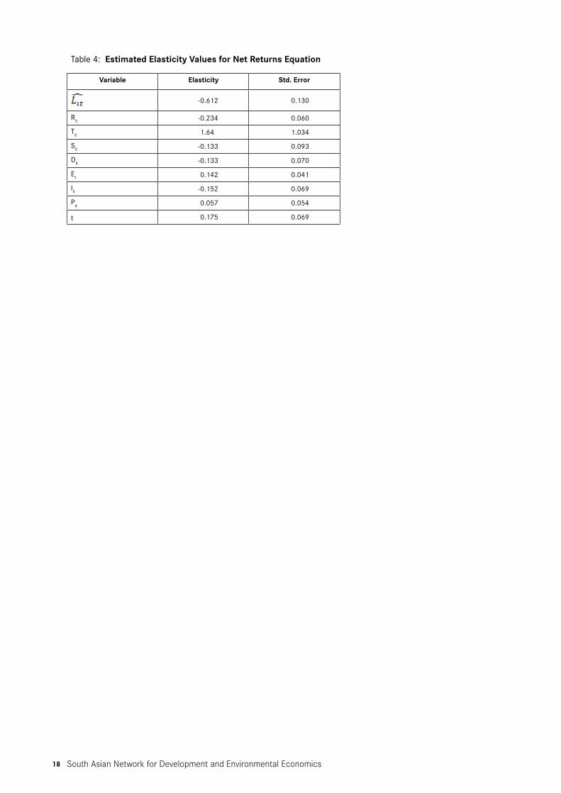
South Asian Network for Development and Environmental Economics18
Table 4: Estimated Elasticity Values for Net Returns Equation
Variable Elasticity Std. Error
-0.612 0.130
Rit -0.234 0.060
Tit 1.64 1.034
Sit -0.133 0.093
Dit -0.133 0.070
Et 0.142 0.041
Iit -0.152 0.069
Pit 0.057 0.054
t 0.175 0.069
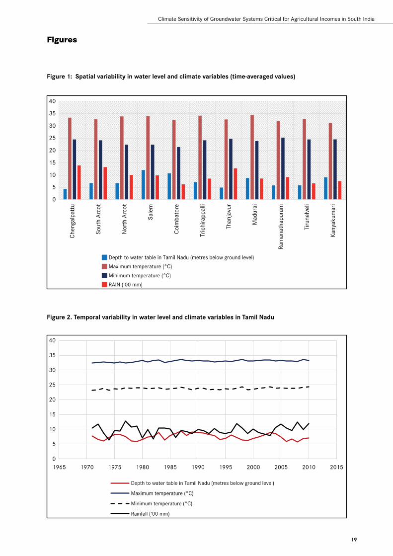
19
Climate Sensitivity of Groundwater Systems Critical for Agricultural Incomes in South India
0
5
10
15
20
25
30
35
40
Chen
galp
attu
Sout
h Ar
cot
Nor
th A
rcot
Sale
m
Coim
bato
re
Tric
hira
ppal
li
Than
javu
r
Mad
urai
Ram
anat
hapu
ram
Tiru
nelv
eli
Kany
akum
ari
Depth to water table in Tamil Nadu (metres below ground level)
Maximum temperature (°C)
Minimum temperature (°C)
RAIN ('00 mm)
0
5
10
15
20
25
30
35
40
1965 1970 1975 1980 1985 1990 1995 2000 2005 2010 2015
Depth to water table in Tamil Nadu (metres below ground level)
Maximum temperature (°C)
Minimum temperature (°C)
Rainfall ('00 mm)
Figures
Figure 1: Spatial variability in water level and climate variables (time-averaged values)
Figure 2. Temporal variability in water level and climate variables in Tamil Nadu

South Asian Network for Development and Environmental Economics20


SANDEEP.O. Box 8975, E.P.C 1056, Lalitpur, Nepal
Street address: c/o ICIMOD, Khumaltar, Lalitpur, Nepal
Tel: 977 1 5003222, Fax: 977 1 5003299, Email: [email protected], Web: www.sandeeonline.org
SANDEE Sponsors