Clinical Research:

Sample

Measure(Intervene)

Analyze

Infer

A study can only be as good as the data . . .

-J.M. Bland

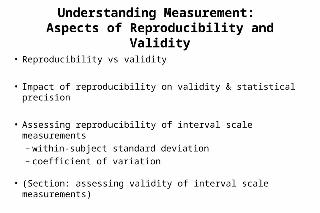
Understanding Measurement: Aspects of Reproducibility and Validity

• Reproducibility vs validity

• Impact of reproducibility on validity & statistical precision

• Assessing reproducibility of interval scale measurements– within-subject standard deviation– coefficient of variation

• (Section: assessing validity of interval scale measurements)

Measurement Scales

Scale Example

Interval continuousdiscrete

weightWBC count

Categoricalordinalnominaldichotomous

tumor stageracedeath

Reproducibility vs Validity

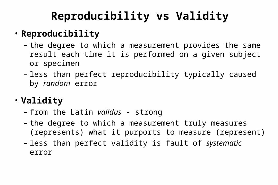
• Reproducibility– the degree to which a measurement provides the same

result each time it is performed on a given subject or specimen

– less than perfect reproducibility typically caused by random error

• Validity– from the Latin validus - strong– the degree to which a measurement truly measures

(represents) what it purports to measure (represent)– less than perfect validity is fault of systematic error

Reproducibility vs Validity

• Reproducibility– aka: reliability, repeatability, precision, variability,

dependability, consistency, stability

• Validity– aka: accuracy

Vocabulary for Error

Overall Inferences from Studies

Individual Measurements

Systematic Error

Validity Validity

(aka accuracy)

Random Error

Precision Reproducibility

Reproducibility and Validity

Good Reproducibility

Poor Validity

Poor Reproducibility

Good Validity

Reproducibility and Validity

Good Reproducibility

Good Validity

Poor Reproducibility

Poor Validity

Why Care About Reproducibility?

Impact on Validity

• Mathematically, the upper limit of a measurement’s validity is a function of its reproducibility

• Consider a study of height and basketball ability:

– Assume height measurement: imperfect reproducibility

– If we had measured height twice on a given person, most of the time we get two different values; at least 1 of the 2 values must be wrong (imperfect validity)

– If study measures everyone only once, errors, despite being random, will lead to biased inferences when using these measurements (i.e. lack validity)

GoodB-Ball

PoorB-Ball

>6 ft 10 30 40 +1 10 +3 30<6 ft 10 50 60 10 +1 50 +5

20 80 100 20 80

P

GoodB-Ball

PoorB-Ball

>6 ft 10 32 42<6 ft 10 48 58

20 80 100

Truth = Prevalence Ratio= (10/40) / (10/60) = 1.5

Observed = Prevalence Ratio = (10/42) / (10/58) = 1.38

10% Misclassification

Impact of Reproducibility on Statistical Precision

• Classical Measurement Theory:

–observed value (O) = true value (T) + measurement error (E)

–If we assume E is random and normally distributed:

E ~ N (0, 2E)

Fra

ctio

n

error-3

0

.02

.04

.06

Error-2 -1 0 1 2 3

Impact of Reproducibility on Statistical Precision

• Assume:–observed value (O) = true value (T) + measurement error (E)

–E is random and ~ N (0, 2E)

• Then, when measuring a group of subjects, the variability of observed values (2

O ) is a combination of:

the variability in their true values (2T )

and

the variability in the measurement error (2E)

2O = 2

T + 2E

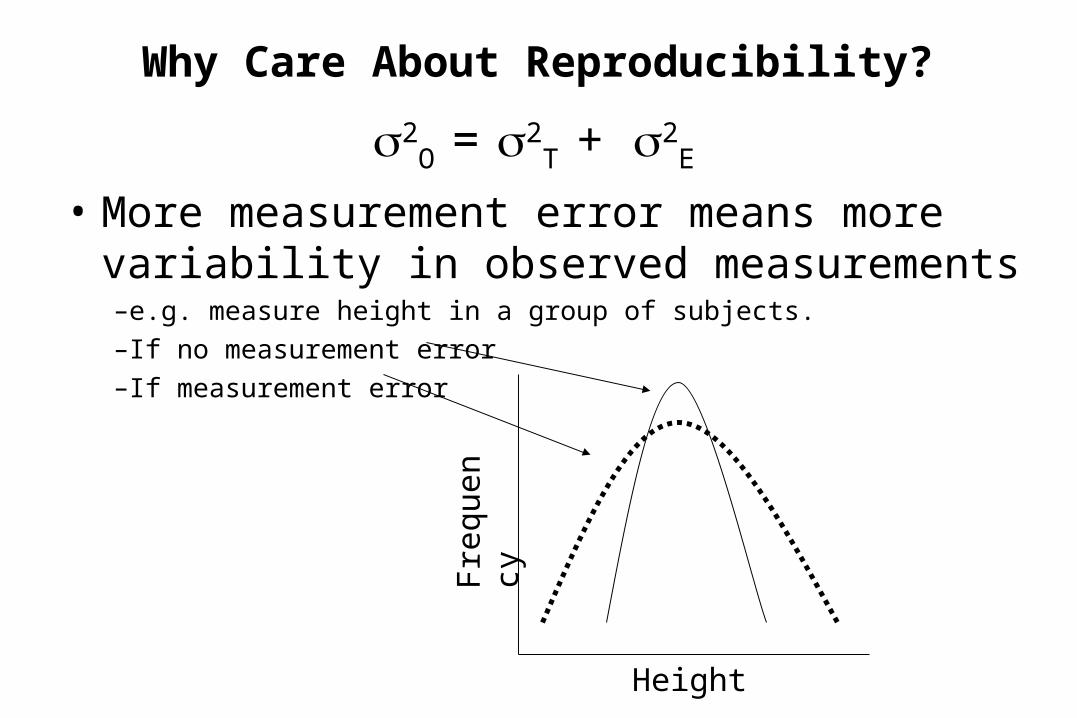
Why Care About Reproducibility?

2O = 2

T + 2E

• More measurement error means more variability in observed measurements–e.g. measure height in a group of subjects. –If no measurement error–If measurement error

Height

Fre

quen

cy

More variability of observed measurements has profound influences on statistical precision/power

2O = 2

T + 2E

• Descriptive studies: wider confidence intervals

• Analytic studies (Observational/RCT’s): power to detect a exposure (treatment) difference is reduced

truth truth + error

truth truth + error

Mathematical Definition of Reproducibility

• Reproducibility

• Varies from 0 (poor) to 1 (optimal)

• As 2E approaches 0 (no error), reproducibility

approaches 1

• Note: we can never directly measure this

2

E

2

T

2

T

2

O

2

T

Simulation study looking at the association of a given risk factor and a certain disease.

Truth is a risk ratio= 2.0

R= reproducibility

Power: probability of estimating a risk ratio within 15% of 2.0

Phillips and Smith, J Clin Epi 1993

Power

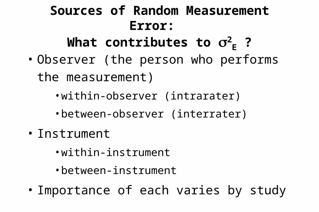
Sources of Random Measurement Error: What contributes to 2

E ?

• Observer (the person who performs the

measurement)

• within-observer (intrarater)

• between-observer (interrater)

• Instrument

• within-instrument

• between-instrument

• Importance of each varies by study

Sources of Measurement Error

• e.g., plasma HIV viral load

– observer: measurement to measurement differences in tube filling, time before processing

– instrument: run to run differences in reagent concentration, PCR cycle times, enzymatic efficiency

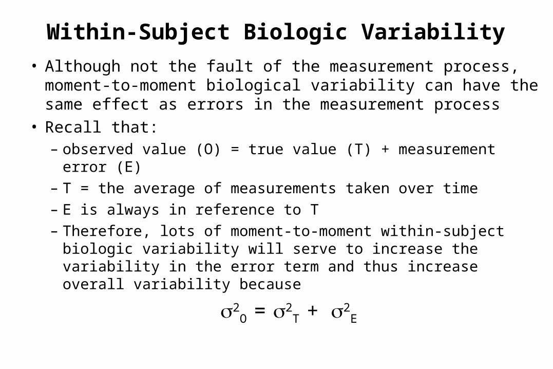
Within-Subject Biologic Variability

• Although not the fault of the measurement process, moment-to-moment biological variability can have the same effect as errors in the measurement process

• Recall that:– observed value (O) = true value (T) + measurement error (E)

– T = the average of measurements taken over time

– E is always in reference to T

– Therefore, lots of moment-to-moment within-subject biologic variability will serve to increase the variability in the error term and thus increase overall variability because

2O = 2

T + 2E

error

Assessing Reproducibility

Depends on measurement scale

• Interval Scale– within-subject standard deviation and derivatives– coefficient of variation

• Categorical Scale

– Kappa (see Clinical Epidemiology course)

– (can be used for both predictors and outcomes)

Reproducibility of an Interval Scale Measurement: Peak Flow

• Assessment requires

>1 measurement per subject

• Peak Flow Rate in 17 adults

(Bland & Altman)

Subject Meas. 1 Meas. 21 494 4902 395 3973 516 5124 434 4015 476 4706 557 6117 413 4158 442 4319 650 638

10 433 42911 417 42012 656 63313 267 27514 478 49215 178 16516 423 37217 427 421

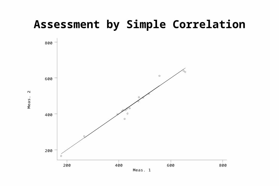
Assessment by Simple CorrelationM

eas.

2

Meas. 1200 400 600 800

200

400

600

800

Pearson Product-Moment Correlation Coefficient

• r (rho) ranges from -1 to +1

• r

• r describes the strength of linear association

• r2 = proportion of variance (variability) of one variable accounted for by the other variable

22 )()())((YYXXYYXX

r = -1.0

r = 0.8 r = 0.0

r = 1.0

r = 1.0 r = -1.0

r = 0.8 r = 0.0

Correlation Coefficient for Peak Flow Data

r ( meas.1, meas. 2) = 0.98

Limitations of Simple Correlation for Assessment of Reproducibility

• Depends upon range of data– e.g. Peak Flow

• r (full range of data) = 0.98• r (peak flow <450) = 0.97• r (peak flow >450) = 0.94

Additional Limitations of Simple Correlation for Assessment of Reproducibility

• Depends upon ordering of data

– get different rho depending upon classification of

meas 1 vs 2

• Measures linear association only

– it would be amazing if the replicates weren’t related

Meas.

2

Meas 1100 300 500 700 900 1100 1300 1500 1700

100

300

500

700

900

1100

1300

1500

1700

Final Limitation of Simple Correlation for Assessment of Reproducibility

• Gives no meaningful parameter using the

same scale as the original measurement

– What does rho = 0.7 vs 0.8 vs 0.9 mean in the

context of peak flow data which ranges from 200

to 600?

– (Note: rho is not “R” from prior slide)

Within-Subject Standard Deviation

• Common (or mean) within-subject standard deviation (sw)

= 15.3 l/min

subject meas1 meas2 mean s1 494 490 492 2.832 395 397 396 1.413 516 512 514 2.83. . . . .. . . . .. . . . .

15 178 165 172 9.1916 423 372 398 36.0617 427 421 424 4.24

17)24.4...83.2( 222

n

si i

sw: Further Interpretation

• If assume that replicate results:– are normally distributed

– mean of replicates estimates true value

• 95% of replicates are within (1.96)(sw) of true valueMeasured Value

x true value

sw

(1.96) (sw)

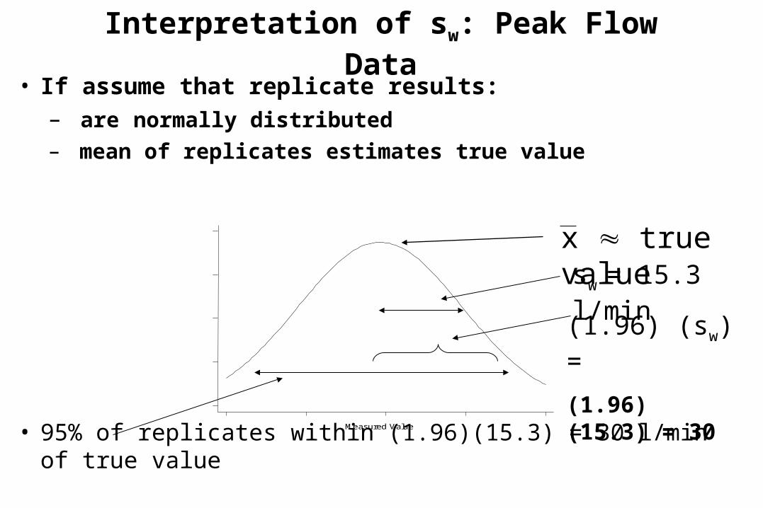
Interpretation of sw: Peak Flow Data

• If assume that replicate results:– are normally distributed

– mean of replicates estimates true value

• 95% of replicates within (1.96)(15.3) = 30 l/min of true valueMeasured Value

x true value

sw = 15.3 l/min

(1.96) (sw) =

(1.96) (15.3) = 30

sw: Further Interpretation

• Difference between any 2 replicates for same person = diff = meas1 - meas2

• Because var(diff) = var(meas1) + var(meas2), therefore,

s2diff = sw

2 + sw2 = 2sw

2

sdiff

1.41s s2s2s ww2w

2diff

Interpreting sw: Difference Between Two Replicates

• If assume that differences:– are normally distributed and mean of differences is 0

– sdiff estimates standard deviation

• The difference between 2 measurements for the same subject is expected to be less than (1.96)(sdiff) = (1.96)(1.41)sw = 2.77sw for 95% of all pairs of measurements

Measured Value

xdiff 0

sdiff

(1.96) (sdiff)

sw: Further Interpretation:The Repeatability Value

• For Peak Flow data:

• The difference between 2 measurements for the same subject is expected to be less than 2.77sw

=(2.77)(15.3) = 42.4 l/min for 95% of all pairs

• i.e. the difference between 2 replicates may be as much as 42.4 liters just by random measurement error alone.

• 42.4 liters termed (by Bland-Altman): “repeatability” or “repeatability coefficient” of measurement

Interpreting the “Repeatability” Value: Is 42.4 liters a lot? Depends upon the context

Clinical management• If other gold standards exist that are more reproducible, and:

– differences < 42.4 are clinically relevant, then 42.4 is bad– differences < 42.4 not clinically relevant, then 42.4 not bad

• If no gold standards, probably unwise to consider differences as much as 42.4 to represent clinically important changes– would be valuable to know “repeatability” for all clinical tests

Research• Depends upon the differences in peak flow you hope to detect

– If ~40, you’re in trouble– If several hundred, then not bad

One Common Underlying sw

• Appropriate only if there is one sw

• i.e, sw does not vary with true underlying value

Wit

hin

-Su

bje

ct

Std

Devia

tion

Subject Mean Peak Flow

100 300 500 7000

10

20

30

40 correlation coefficient = 0.17, p = 0.36

Another Interval Scale Example

• Salivary cotinine in children (Bland-Altman)

• n = 20 participants measured twicesubject trial 1 trial 2

1 0.1 0.12 0.2 0.13 0.2 0.3. . .. . .. . .

18 4.9 1.419 4.9 3.920 7.0 4.0

Cotinine: Absolute Difference vs. MeanS

ub

ject

Ab

solu

te D

iffe

ren

ce

Subject Mean Cotinine0 2 4 6

0

1

2

3

4 correlation = 0.62,

p = 0.001

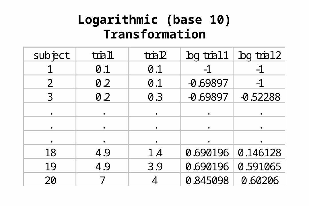
Logarithmic (base 10) Transformation

subject trial1 trial2 log trial 1 log trial 21 0.1 0.1 -1 -12 0.2 0.1 -0.69897 -13 0.2 0.3 -0.69897 -0.52288. . . . .. . . . .. . . . .

18 4.9 1.4 0.690196 0.14612819 4.9 3.9 0.690196 0.59106520 7 4 0.845098 0.60206

Log10 Transformed: Absolute Difference vs. MeanS

ub

ject

ab

s lo

g d

iff

Subject mean log cotinine-1 -.5 0 .5 1

0

.2

.4

.6 correlation = 0.07 p=0.7

sw for log-transformed cotinine data

• sw

• because this is on the log scale, it refers to a multiplicative factor and hence is known as the geometric within-subject standard deviation

• it describes variability in ratio terms (rather than absolute numbers)

units log .. 10175003050

Interpretation of sw: Cotinine Data

• If assume that replicate results:– are normally distributed

– mean of replicates estimates true value

• 95% of replicates within a factor of 0.34 log10 of true valueMeasured Value

x true value

sw = 0.175 log10

(1.96) (sw) =

(1.96) (0.175) = 0.34

Interpretation of sw: Cotinine Data

• 95% of replicates are within a factor of 0.34 log10 of true value

• back-transforming to base10 scale:

– antilog(0.34) = 10 0.34 = 2.2• 95% of replicates are within a factor of 2.2 of true value• An observed cotinine value of 2 ng/ml would tell us that the

true value may be:– as little as 2/2.2 = 0.9– as big as 2*2.2 = 4.4– just by measurement error alone

Interpretation of sw: Cotinine DataRepeatability

• The difference between 2 measurements for the same subject is expected to be less than a factor of (1.96)(sdiff) = (1.96)(1.41)sw = 2.77sw for 95% of all pairs of measurements

• For cotinine data, sw= 0.175 log10, therefore:

– 2.77*0.175 = 0.48 log10– back-transforming, antilog(0.48) = 10 0.48 = 3.1

• For 95% of all pairs of measurements, the ratio between the measurements may be as much as 3.1 fold (this is “repeatability”)

Coefficient of Variation• For cotinine data, the within-subject standard deviation (on the

native scale) varies with the level of the measurement

• If the within-subject standard deviation is proportional to the level of the measurement, this can be summarized as:

coefficient of variation =

= 1.49 -1 = 0.49

• At any level of cotinine, the within-subject standard deviation of repeated measures is 49% of the level

meansubject -withindeviation standardsubject -within

1- )antilog(sw

Coefficient of Variation for Peak Flow Data

• By definition, when the within-subject standard deviation is not proportional to the mean value, as in the Peak Flow data, then there is not a constant ratio between the within-subject standard deviation and the mean.

• Therefore, there is not one common coefficient of variation

• Estimating the the “average” coefficient of variation (within-subject sd/overall mean) is not meaningful

Peak Flow Data: Use of Coefficient of Variation when sw is Constant

Mean of replicates sw C.V.100 15.3 0.153200 15.3 0.077300 15.3 0.051400 15.3 0.038500 15.3 0.031600 15.3 0.026700 15.3 0.022

Could report a family of CV’s but this is tedious

Pattern of within-subject standard deviation over range of measurement

Which Index to Use?

Constant

within-subject standard deviation (and derivatives like repeatability)

Proportional to the magnitude of the measurement

geometric within-subject standard deviation (and derivatives like repeatability)

Coefficient of variation Neither constant nor porportional

Break range of data into pieces where there is consistent behavior; report family of within-subject standard deviations & coefficients of variation

Assessing Validity

• Measures can be assessed for validity in 3 ways:

– Content validity• Face• Sampling

– Construct validity– Empirical validity (aka criterion)

• Concurrent (i.e. when gold standards are present)– Interval scale measurement: 95% limits of agreement– Categorical scale measurement: sensitivity & specificity

• Predictive

Conclusions• Measurement reproducibility plays a key role in determining validity and

statistical precision in all different study designs

• When assessing reproducibility, for interval scale measurements:

• avoid correlation coefficients

• use within-subject standard deviation and derivatives like

“repeatability”

• or coefficient of variation if within-subject sd is proportional to the

magnitude of measurement

• (For categorical scale measurements, use Kappa)

• What is acceptable reproducibility depends upon desired use

• Assessment of validity depends upon whether or not gold standards are

present, and can be a challenge when they are absent