PHYSICAL REVIEW A 89, 052133 (2014)

Closed-form solution of Lindblad master equations without gain

Juan Mauricio Torres*

Theoretische Physik, Universitat des Saarlandes, 66123 Saarbrucken, Germany, Institut fur Angewandte Physik, Technische UniversitatDarmstadt, 64289 Darmstadt, Germany and Departamento de Investigacion en Fısica, Universidad de Sonora, 83000 Hermosillo, Mexico

(Received 11 January 2013; published 30 May 2014)

We present a closed-form solution to the eigenvalue problem of a class of master equations that describe openquantum systems with loss and dephasing but without gain. The method relies on the existence of a conservednumber of excitations in the Hamiltonian part and the fact that none of the Lindblad operators describe anexcitation of the system. In the absence of dephasing Lindblad operators, the eigensystem of the Liouvilleoperator can be constructed from the eigenvalues and eigenvectors of the effective non-Hermitian Hamiltonianused in the quantum jump approach. Open versions of spin chains, the Tavis-Cummings model, and coupledHarmonic oscillators without gain can be solved using this technique.

DOI: 10.1103/PhysRevA.89.052133 PACS number(s): 03.65.Fd, 03.65.Yz

I. INTRODUCTION

Master equations in Lindblad form provide the mostgeneral dynamical description of open quantum systemsunder the Markov assumption [1–3]. Sometimes also calledKossakowski-Lindblad equations, due to pioneering worksof Kossakowski [4,5], these type of equations have beenextensively used to describe atom cooling [6], decoherencein quantum information theory and quantum engineering ofstates [7,8].

Many Hamiltonian systems have been extended to includedissipation in Lindblad form; however, even if the Hamiltonianpart of the system is solvable, the full solution to the dissipativeversion is not obvious. The problem results from the factthat the Liouville operator governing the dynamics is anon-Hermitian operator which acts on density matrices. Effortshave been made to tackle this problem and, while thereexist analytical steady-state solutions to some problems [9],there are not many solutions to the eigenvalue problem ofspecific systems. The dissipative version of the Harmonicoscillator, up to two spins, and the Jaynes-Cummings (JC)model are the only open systems for which exact solutionsof the eigenvalue problem are known [10–15]. The solutionsto the Jaynes-Cummings model that can be found in theliterature [10,14] are examples that show how intricate thecalculation of the eigensystem of the Liouville operator canbe. In particular, the work of Briegel and Englert [10] solvesthis problem in terms of the eigenbases of the uncoupledsubsystems which are formed by a damped harmonic oscillatorand a damped two-level atom. The interaction part operates ina nontrivial way on the elements of these combined bases and,therefore, although manageable in this case, this procedure isnot suitable to generalize to higher dimensional systems as itwould lead to very tedious calculations.

In this work we present a systematic method for solvingthe eigenvalue problem of a broad class of Lindblad masterequations which do not involve any form of gain and that sharethe characteristic of being solvable in the Hamiltonian part withan additional constant of motion that measures the number ofexcitations in the system. Under these assumptions we are

*mauricio.torres@physik.tu-darmstadt.de

able to find the eigenvalues and the eigenbasis of the operatorthat is obtained by subtracting from the Liouville operator,the jump operator of the quantum jumps approach [2,16]. Weuse an expansion in terms of the elements of this basis tosolve for the eigensystem of the complete Liouville operatorand obtain a first-order vector recurrence relation that canbe solved in an iterative way. In the absence of dephasingLindblad operators, the eigensystem of the full Liouvilliancan be constructed in a systematic way from the eigensystemof the non-Hermitian Hamiltonian of the quantum jumpsapproach. Specifically, it is shown that each eigenvalue of thecomplete system is proportional to the sum of two eigenvaluesof the corresponding non-Hermitian Hamiltonian. The maindifference with respect to the procedure used in [10] is thatwe use the eigenbasis of the part of the master equationwithout the jump operator, instead of the eigenbasis withoutthe interaction term. With this approach we are able toreproduce previous specific solutions to the damped harmonicoscillator [11] and the damped Jaynes-Cummings model [10],but most importantly our method is presented in a generalway that encompasses systems such as the dissipative versionof Heisenberg XXZ spin chains [17], the Affleck-Kennedy-Lieb-Tasaki (AKLT) model [18], the Bose-Hubbard model [7],the Tavis-Cummings model [19], etc. Our construction isperformed for systems that do not present any source of gain;nevertheless, similar arguments lead to exact solutions foranalog systems without loss.

The paper is organized as follows. In Sec. II we formalizethe assumptions that define the class of systems we want toaddress. Furthermore, we show the procedure to solve theeigensystem of the master equation in terms of the eigensystemof an effective non-Hermitian Hamiltonian. In Sec. III weconsider systems that include dephasing Lindblad operatorsand explain how to solve this class of systems in connectionto the method presented in Sec. II. Finally, in Sec. IV wepresent two examples of systems that can be solved using thistechnique: The Jaynes-Cummings model and the two-atomsTavis-Cummings model. As an application we evaluate theatomic spontaneous emission spectrum of the first example.

II. THE MASTER EQUATION

We consider systems whose dynamics are governed by amaster equation, which consists of a coherent Hamiltonian

1050-2947/2014/89(5)/052133(9) 052133-1 ©2014 American Physical Society

JUAN MAURICIO TORRES PHYSICAL REVIEW A 89, 052133 (2014)

evolution and a dissipative part in Lindblad form. Thedynamical equation is given in terms of the so-called Liouvilleoperator as

Lρ = 1

i�[H,ρ] +

∑s

γs

2(2AsρA†

s − A†sAsρ − ρA†

sAs). (1)

Concerning the Hamiltonian part we assume that no sourceof driving is present in the system and that an observable I

exists which commutes with H . This additional constant ofmotion may be interpreted as a measure of the excitationsin the system. Furthermore, we consider that the system isdefined on a Hilbert space H and that there exists a completebasis set {|n,j 〉} with N elements. In this basis I is diagonaland there are dn states with the same integer eigenvalue of I ,that is, I |n,j 〉 = n|n,j 〉, with n = 0, . . . N andN = ∑N

n=0 dn.We make all the treatment for finite N , but under the same lineof thought of [10,11,15] the results also apply in the limit N →∞, which also implies the limit ofN → ∞, for countable infi-nite separable Hilbert spaces. As an immediate consequence ofthe existence of the conserved quantity I we can identify thatthe Hamiltonian has a block-diagonal form in the basis where I

is diagonal, with each block H (n) of size dn × dn. This featureis essential and will be exploited in our construction.

For the dissipative part, we first consider only Lindbladoperators As which describe losses in the system. We formalizethis condition with the commutation relation

[As,I ] = As. (2)

If we were considering the Jaynes-Cummings model [20], wecould take the electromagnetic mode annihilation operator a

and the spin lowering operator σ− as Lindblad operators, cor-responding to the situation in which the system interacts witha zero-temperature reservoir. In this example, the additionalconstant of motion would be a†a + σ+σ−.

From the previous consideration it follows that eachHermitian operator A

†sAs also commutes with I , which implies

a block-diagonal form in the basis where I is diagonal.This motivates rewriting the master equation in two parts,one that conserves the excitations and the other describingthe de-excitation of the system. With the introduction of thenon-Hermitian Hamiltonian

K = H − i�∑

s

γs

2A†

sAs, (3)

which can be recognized as the effective Hamiltonian usedin the quantum trajectories technique [2,16], one can rewriteEq. (1) as the sum of the following two parts Lρ = Kρ + Aρ,with

Kρ = 1

i�(Kρ − ρK†), Aρ =

∑s

γsAsρA†s . (4)

The first term describes the part of the dynamics that conservesexcitation, while the second one, the jump operator, describesthe de-excitations in the system.

In order to solve the master equation, our strategy will be tofind the eigensystem of K. Then, we will deduce how the jumpoperator acts on each of its eigenvectors. Making a plausibleansatz for the eigenvectors of the complete master equation as asuperposition of the eigenvectors of K and then inserting them

into the full master equation will allow us to find a solvablerecursion relation for the coefficients of the superposition.

A. Eigensystem of K

Given the fact that [K,I ] = 0 it follows that K|n,k〉 =∑dn

j=1 K(n)j,k|n,j 〉, i.e., it does not couple eigenvectors of I with

different values of n. In the basis {|n,j 〉}, K has a block-diagonal form, with each block given by a matrix of sizedn × dn. We assume that each block can be diagonalized bythe transformation

K (n) = Q†(n)K (n)R(n), with Q†(n)R(n) = Idn, (5)

where K (n) is a diagonal matrix with the eigenvalues of thenth block in its diagonal and Idn

is the identity matrix ofdimension dn. We use a tilde throughout this paper to denotewhen a matrix is expressed in the eigenbasis of K . The dn × dn

matrices Q†(n) and R(n) are the blocks of the operators Q† andR which diagonalize the operator K . The columns (rows) ofR (Q†) are the right (left) eigenvectors of K [21] and in theoriginal basis {|n,j〉} they can be expanded as

∣∣rnj

⟩ =dn∑

k=1

R(n)k,j |n,k〉, ∣∣qn

j

⟩ =dn∑

k=1

Q(n)k,j |n,k〉. (6)

One can verify that these states are also eigenstates of I , i.e.,I |rn

j 〉 = n|rnj 〉, and assuming that the transformation in Eq. (5)

exists it follows that they are orthogonal and complete:

⟨qn

k

∣∣rmj

⟩ = δk,j δn,m,

N∑n=0

dn∑j=1

∣∣rnj

⟩⟨qn

j

∣∣ = I. (7)

The eigenvalue equation for K is then

K∣∣rn

j

⟩ = ε(n)j

∣∣rnj

⟩, K†∣∣qn

j

⟩ = ε∗(n)j

∣∣qnj

⟩, (8)

with the complex eigenvalues ε(n)j .

B. Eigensystem of KThe eigensystem of the operator K can be constructed from

the eigensystem of the non-Hermitian Hamiltonian K . It canbe verified by inspection of Eq. (4) that the elements

�(l,n)j,k = ∣∣rn+l

j

⟩⟨rnk

∣∣, �(l,n)j,k = ∣∣qn+l

j

⟩⟨qn

k

∣∣, (9)

with j = 1, . . . dn+l and k = 1, . . . dn, are the right and lefteigenvectors of K and that they solve the eigenvalue equation

K�(l,n)j,k = λ

(l,n)j,k �

(l,n)j,k , K†�(l,n)

j,k = λ∗(l,n)j,k �

(l,n)j,k , (10)

with eigenvalues

λ(l,n)j,k = 1

i�

[ε

(n+l)j − ε

∗(n)k

]. (11)

The dual operator of K is given by K†ρ = 1i�

(ρK −K†ρ) [10,11]. From Eq. (7), it follows that these eigenvectorsare orthogonal with respect to the Hilbert-Schmidt innerproduct:

Tr{(

�(l,n)j,k

)†�

(l′,n′)j ′,k′

} = δn,n′δl,l′δj,j ′δk,k′ . (12)

Now, let us study in more detail the operator K and howit acts on the elements |n + l,j 〉〈n,k| with n + l,n = 0 . . . N ,

052133-2

CLOSED-FORM SOLUTION OF LINDBLAD MASTER . . . PHYSICAL REVIEW A 89, 052133 (2014)

j = 1 . . . dn+l and k = 1, . . . dn. These elements form a basisfor the vector spaceB(H) of the operators that act on the Hilbertspace H. As K does not couple basis elements of different n

it follows that K does not couple elements with different pairsof excitation numbers n + l and n, that is,

K|n + l,j ′〉〈n,k′| =dn+l ,dn∑j,k=1

K(l,n)j,k,j ′,k′ |n + l,j 〉〈n,k|. (13)

This shows that the operator K is formed by the uncoupledblocks K(l,n), where each one of them can be represented by atensor of rank 4 and dimensions dn+l × dn × dn+l × dn.

To simplify the evaluation we will adopt the followingbijective mapping of indices j,k → ν, with

ν = dn(j − 1) + k, ν = 1 . . . Dl,n = dn+ldn. (14)

In this convention that maps two indices to one, the tensor inEq. (13) can now be expressed as a Dl,n × Dl,n matrix that actson vectors of size Dl,n which are obtained by vectorizing rowby row a matrix of size dn+l × dn using the mapping of indicesin Eq. (14). With this convention and using the properties ofthe tensor product, we can express the blocks of K as

K(l,n) = 1

i�(K (n+l) ⊗ Idn

− Idn+l⊗ K∗(n)). (15)

Analogous to Eq. (5), there exists a transformation whichdiagonalizes each block of K. It has the form

K(l,n) = Q†(l,n)K(l,n)R(l,n), Q†(l,n)R(l,n) = IDl,n. (16)

The eigenvectors of K, given in Eq. (9), provide us with thetransformation that diagonalizes each of its blocksK(l,n), givenby the tensor product of the matrices with the eigenvectors ofK , i.e.,

Q(l,n) = Q(n+l) ⊗ Q∗(n),

R(l,n) = R(n+l) ⊗ R∗(n). (17)

C. Jump operator

We proceed to study the action of the jump operator A onthe eigenvectors ofK. As it is formed by the Lindblad operatorsAs we first focus on how these act on the eigenvectors of thenon-Hermitian Hamiltonian K . We assume that the action ofeach As on states in the original basis is known. Considering itscommutation relation with I given in Eq. (2) we can deducethat it is of the form As |n,j 〉 = ∑dn−1

k=1 A(n)s;k,j |n − 1,k〉. It is

manifested in this way that every As connects states of theblock n to states in the block n − 1, meaning that the Lindbladoperators are also composed of uncoupled blocks A(n)

s ofdimension dn−1 × dn. Using the transformations of Eq. (5)it is possible to transform these blocks to the representation inthe eigenbasis of K in the following way:

A(n)s = Q†(n−1)A(n)

s R(n). (18)

Thereby, we find that the action of the Lindblad operators ontothe right eigenstates of K can be expressed as

As

∣∣rnj

⟩ =dn−1∑k=1

A(n)s;k,j

∣∣rn−1k

⟩. (19)

With the blocks of the Lindblad operators in the represen-tation of the eigenbasis of K it is now possible to build theblocks of the jump operator using the tensor product. Theyhave the form

A(l,n) =∑

s

γsA(n+l)s ⊗ A∗(n)

s (20)

and they are matrices of size Dl,n−1 × Dl,n that connectvectorized matrices of dimension Dl,n to others of dimensionDl,n−1. It is in this representation that one can identify how thejump operator acts on the eigenbasis of K, that is,

A�(l,n)ν =

Dl,n−1∑ν ′

A(l,n)ν ′,ν �

(l,n−1)ν ′ . (21)

Analogously we can find the corresponding equation for thedual jump operator acting on the left eigenvectors as

A†�(l,n)ν =

Dl,n+1∑ν ′

A∗(l,n+1)ν,ν ′ �

(l,n+1)ν ′ . (22)

We have adopted the mapping of indices in Eq. (14) to labelthe eigenvectors of K and we introduced the dual of the jumpoperator, defined as A†ρ = ∑

s γsA†sρAs .

In an alternative calculation one could start with theevaluation of the blocks A(l,n) in the original basis based onthe blocks A(n)

s , in the same manner as in Eq. (20). Then onecould change the basis using the transformation of Eq. (17) tofind

A(l,n) = Q†(l,n−1)A(l,n)R(l,n). (23)

D. Eigensystem of the full master equation

Noting that the jump operator Eq. (21) couples eigenvectorsof K of definite excitation number n with a superposition ofeigenvectors of n − 1 without changing the value of l, it seemsreasonable to take as an ansatz for the eigenvectors of the fullLiouvillian L a superposition of eigenvectors of K with a fixedvalue of l. The proposed ansatz, in the vectorized conventionis ρl, = ∑

n,ν vl,;nν �(l,n)

ν , where is an eigenvalue of the fullmaster equation and for the moment it labels the eigenvectorsand its coefficients. Our next step is to study how the fullLiouvillian L acts on these type of states. From Eqs. (10), (14),and (21) one obtains

Lρl, = ρl, =N∑

n=0

Dl,n∑ν=1

vl,;nν λ(l,n)

ν �(l,n)ν

+N∑

n=1

Dl,n,Dl,n−1∑ν,ν ′=1

vl,;nν A(l,n)

ν ′,ν �(l,n−1)ν ′ . (24)

Reordering of indices and matching the elements �(l,n)ν leaves

us with the following recurrence relation for the coefficientsat fixed n:

( − λ(l,n)

ν

)vl,;n

ν =Dl,n+1∑

ν ′A(l,n+1)

ν,ν ′ vl,;n+1ν ′ . (25)

The relation holds for any complex value of , but we take thesimplest one in which the recurrence ends, using a similar

052133-3

JUAN MAURICIO TORRES PHYSICAL REVIEW A 89, 052133 (2014)

reasoning as in [11]. We find that the eigenvalues for thecomplete Liouville operator are = λ(l,m)

μ , for certain m andμ which label inner blocks in the same way as ν. This resulttells us that L and K have the same spectrum, a fact that canalso be understood as L has an upper triangular form in thebasis where K is diagonal. Another observation is that forn = m the left-hand side of Eq. (25) vanishes, which meansthat all coefficients are zero for n > m. The first nonvanishingcoefficient is vl,;m

μ = 1. From here one can proceed to evaluatethe rest of the coefficients in a recursive way. Note also thatthree integers are needed to define each eigenvector: m, μ,and l (or four if instead one uses μ → (j ′′ − 1)dm + k′′ in thematrix representation). Hence, we redefine the coefficients asvl,;n

ν → v(l,m;n)μ;ν .

The recursion relation can also be cast in terms of matrixmultiplication, if one takes a vector of coefficients v(l,m;n)

μ foreach block of n. Let us define the nonzero elements of theDl,n × Dl,n diagonal matrix as

T (l,m;n)μ;ν,ν = (

λ(l,m)μ − λ(l,n)

ν

)−1. (26)

With this definition, the recursion in Eq. (25) can be solved togive the nth vector with Dl,n entries:

v(l,m;n)μ =

(m−1∏i=n

T (l,m;i)μ A(l,i+1)

)e(l,m)μ . (27)

Thereby v(l,m;m)μ = e(l,m)

μ is a column vector of dimensionsDl,m with a one in the μth entry and zero elsewhere. Allthe coefficients for n > m vanish. Now one can write the righteigenvectors of the full Liouvillian as

ρ(l,m)μ =

m∑n=0

Dl,n∑ν=1

v(l,m;n)μ;ν �(l,n)

ν . (28)

The left eigenvectors can be evaluated in a similar wayand as we already know the eigenvalues of L we can use asuperposition of the left eigenvectors of K with fixed l to find

L†ρ(l,m)μ = λ∗(l,m)

μ ρ(l,m)μ =

N∑n=0

Dl,n∑ν=1

u(l,m;n)μ;ν λ∗(l,n)

ν �(l,n)ν

+N−1∑n=0

Dl,n,Dl,n+1∑ν,ν ′=1

u(l,m;n)μ;ν A∗(l,n+1)

ν,ν ′ �(l,n+1)ν ′ . (29)

Again, reordering indices and matching the coefficients foreach �(l,m)

ν we find the recursion relation

(λ∗(l,m)

μ − λ∗(l,n)ν

)u(l,m;n)

μ;ν =Dl,n−1∑ν ′=1

A∗(l,n)ν ′,ν u

(l,m;n−1)μ;ν ′ , (30)

which can be iterated to give the solution for the coefficientsas

u(l,m;n)μ =

(m∏

i=n−1

T †(l,m;i+1)μ A†(l,i+1)

)e(l,m)μ . (31)

In this way, we find the following expression for the lefteigenvectors:

ρ(l,m)μ =

N∑n=m

Dl,n∑ν=1

u(l,m;n)μ;ν �(l,n)

ν . (32)

To express the eigenvectors of the full Liouvillian in theoriginal basis, one can apply the transformation in Eq. (17)one by one to each of the vectors in Eqs. (27) and (31) as

v(l,m;n)μ = R(l,n)v(l,m;n)

μ , u(l,m;n)μ = Q(l,n)u(l,m;n)

μ . (33)

Using the mapping of indices in Eq. (14), one finally finds theleft and right set of eigenvectors in the original basis:

ρ(l,m)j,k =

m∑n=0

dn+l ,dn∑j ′,k′=1

v(l,m;n)j,k;j ′,k′ |n + l,j ′〉〈n,k′|,

ρ(l,m)j,k =

N∑n=m

dn+l ,dn∑j ′,k′=1

u(l,m;n)j,k;j ′,k′ |n + l,j ′〉〈n,k′|. (34)

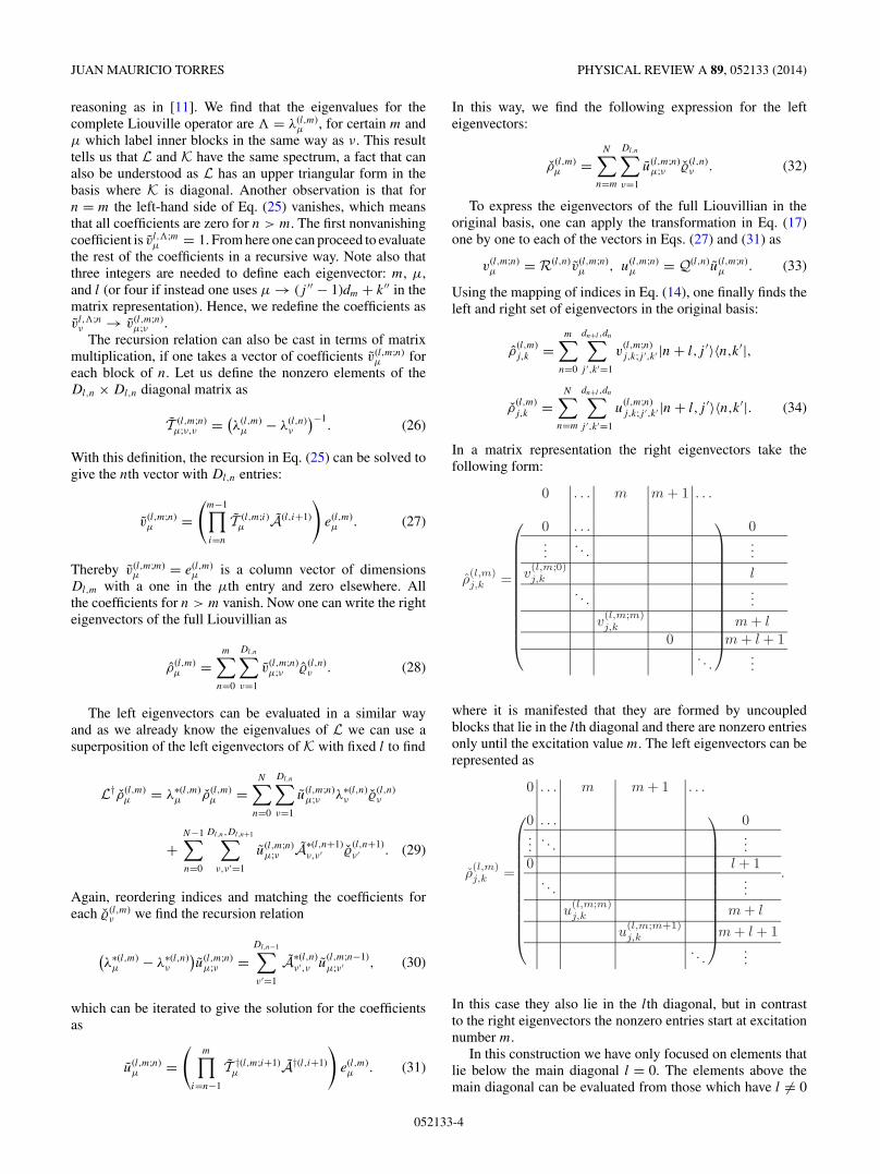
In a matrix representation the right eigenvectors take thefollowing form:

ρ(l,m)j,k =

0 . . . m m + 1 . . .

⎛⎜⎜⎜⎜⎜⎜⎜⎜⎜⎜⎜⎝

⎞⎟⎟⎟⎟⎟⎟⎟⎟⎟⎟⎟⎠

0 . . . 0...

. . ....

v(l,m;0)j,k l

. . ....

v(l,m;m)j,k m + l

0 m + l + 1.. .

...

where it is manifested that they are formed by uncoupledblocks that lie in the lth diagonal and there are nonzero entriesonly until the excitation value m. The left eigenvectors can berepresented as

ρ(l,m)j,k =

0 . . . m m + 1 . . .

⎛⎜⎜⎜⎜⎜⎜⎜⎜⎜⎜⎜⎝

⎞⎟⎟⎟⎟⎟⎟⎟⎟⎟⎟⎟⎠

0 . . . 0...

. . ....

0 l + 1.. .

...u

(l,m;m)j,k m + l

u(l,m;m+1)j,k m + l + 1

.. ....

.

In this case they also lie in the lth diagonal, but in contrastto the right eigenvectors the nonzero entries start at excitationnumber m.

In this construction we have only focused on elements thatlie below the main diagonal l = 0. The elements above themain diagonal can be evaluated from those which have l = 0

052133-4

CLOSED-FORM SOLUTION OF LINDBLAD MASTER . . . PHYSICAL REVIEW A 89, 052133 (2014)

by taking the Hermitian adjoint as ρ†(l,m)j,k and ρ

†(l,m)j,k , with

corresponding eigenvalues λ∗(l,m)j,k . Including them completes

a basis set that spans the vector space B(H).

III. INCLUSION OF DEPHASING OPERATORS

In this section we briefly comment on the inclusion ofdephasing Lindblad operators Cs in the master equation. Thesehave the commutation relation [Cs,I ] = 0 with the constantof motion I . Its inclusion results in a Liouville operatorthat we write in the form L = M + A, with M = K + C,which is written in terms of the operators in Eq. (4) and thenew term

Cρ =∑

s

κs

2(2CsρC†

s − C†s Csρ − ρC†

s CS). (35)

The Liouvillian C also preserves the excitation numbers n andl, but cannot be constructed solely out of a non-HermitianHamiltonian because of the dephasing term

∑s κsCsρC

†s .

Nevertheless, as we have separated the parts of the LiouvillianL that conserves excitations from the jump operator, thediagonalization in this case can be carried out in a similarmanner as it was shown in the previous section. In this casethe diagonalization of the blocks of M is required. These canbe evaluated using Eq. (15) with M(l,n) = K(l,n) + C(l,n) andthe blocks of C which can be constructed as

C(l,n) =∑

s

κs

2

(2C(n+l)

s ⊗ C∗(n)s

− [C†s Cs]

(n+l) ⊗ Idn− Idn+l

⊗ [C†s Cs]

(n)). (36)

Here we have assumed that the action of each Cs ontothe basis {|n,j 〉} is known and so the dn × dn matricesC(n)

s are known. Thereby, the transformations to be foundare those that diagonalize each block as Q†(l,n)M(l,n)R(l,n)

and form the eigenvectors of M. From this point, thediagonalization procedure of the full Liouvillian follows thesame steps as in Sec. II D, with the eigensystem of Kbeing replaced by the eigensystem of M and the blocksof the jump operator evaluated as in Eq. (23). The eigen-values of L are the eigenvalues of the excitation-preservingpart M.

IV. EXAMPLES

In this section we present examples of systems with physicalrelevance that can be solved using the technique introduced inSecs. II and III.

A. Jaynes-Cummings model

The first example we consider is the damped Jaynes-Cummings model, which describes the interaction of a two-level system (TLS) with one mode of the electromagnetic fieldinside an optical cavity [20]. We use this model to test andshow our method and compare with the solution introducedby Briegel and Englert in [10].

The Hamiltonian of the JC model in the interaction picturewith respect to the cavity mode energy is given by

H = �δσ+σ− + �g(aσ+ + a†σ−), (37)

where a and a† are the cavity mode creation and annihilationoperators, and σ± = 1

2 (σx ± iσ y) are the raising and loweringoperators of the two-level system and are defined in terms ofthe Pauli matrices σx , σy , and σ z. The detuning between theTLS frequency gap and the cavity mode is given by δ.

In this case one can recognize that the constant of motionis given by

I = a†a + σ+σ−, (38)

and its eigenbasis {|n,j〉} is given by the states

|n,1〉 = |n〉 ⊗ |g〉, n � 0,

|n,2〉 = |n − 1〉 ⊗ |e〉, n > 0, (39)

with the number state |n〉 describing n photons in the cavityand the atomic excited |e〉 and ground state |g〉. The state |n,2〉is only permissible for n > 0 and so we note that the basisis formed by a singlet state, which is the eigenvector of I

with eigenvalue zero and a family of pairs with eigenvalue n.Therefore, d0 = 1 and dn>0 = 2 in this example.

The Lindblad operators we consider are σ− and a, whichfulfill the commutation relation of Eq. (2). Using them we canconstruct the effective Hamiltonian of Eq. (3), which reads

K = H − i 12 �γ σ+σ− − i 1

2 �κa†a. (40)

It is a non-Hermitian operator which commutes with I , so thatone can write it as a block-diagonal matrix in the basis ofEq. (39), with its blocks given by

K (0) = 0,

K (n>0) = �

(−i nκ2 g

√n

g√

n2δ−i(n−1)κ−iγ

2

). (41)

The eigenvalues can be computed and are given by

ε(n)j = �

2δ − i(2n − 1)κ − iγ

4

+ (−1)j�

√g2n + (2δ + iκ − iγ )2

16. (42)

It can be checked that they are degenerate only in thespecial case δ = 0 and 16g2n = (κ − γ )2. Apart from thiscase, the eigenvalues of each block are different and thediagonalization of the matrices K (n) can be accomplished withthe transformation

R(n>0) =(

cos θn − sin θn

sin θn cos θn

),

θn = arctan

(2ε

(n)1 + i�nκ

2�g√

n

). (43)

In this example Q† = R, because K is a complex symmetricoperator. Together with Eqs. (6) and (39) the right and lefteigenvectors of K can be obtained. For n = 0 no transfor-mation is needed as the singlet |0,1〉 is already an eigenstateof K .

Using Eq. (15) together with Eq. (41) one can build theblocks K(l,n) of the generator K defined in Eq. (4), whichrepresents the part of the Liouvillian L which conserves thenumber of excitations. These blocks can be diagonalized bythe transformation R(l,n) which can be obtained from Eqs. (17)

052133-5

JUAN MAURICIO TORRES PHYSICAL REVIEW A 89, 052133 (2014)

and (43). It is again an orthonormal transformation in thisexample. The eigenvalues of K are also the eigenvalues ofthe full Liouvillian L and can be evaluated from Eq. (11), byinserting the result of Eq. (42).

The Lindblad operators can also be expressed in terms ofblocks in the basis of Eq. (39). They have the following form:

σ−(1) = (0 1

), σ−(n>1) =

(0 1

0 0

),

a(1) = (1 0

), a(n>1) =

(√n 0

0√

n − 1

). (44)

Using them as explained in Sec. II C one can also constructthe blocks of the jump operator A. All the information is nowassembled and the full solution can be obtained as explainedin Sec. II D.

In particular, the part of the eigensystem with lowestexcitation number is given by

ρ(0,0)1,1 = |0,1〉〈0,1|, ρ

(0,0)1,1 = I,

ρ(1,0)j,1 = ∣∣r1

j

⟩〈0,1|, ρ(1,0)j,1 =∣∣q1

j

⟩〈0,1|+ . . . ,

ρ(0,1)j,k = ∣∣r1

j

⟩⟨r1k

∣∣ − ⟨r1k

∣∣r1j

⟩|0,1〉〈0,1|, ρ(0,1)j,k =∣∣q1

j

⟩⟨q1

k

∣∣+ . . . ,

with the corresponding eigenvalues λ(0,0)1,1 = 0, λ

(1,0)j,1 =

−iε(1)j /� and λ

(0,1)j,k = −i(ε(1)

j − ε∗(1)k )/�.

We close this subsection by remarking that our methodcan solve the Jaynes-Cummings model by solving 2 × 2complex matrices which are the blocks of the effectiveHamiltonian widely used in the quantum trajectories approach.The solutions can be manageable at least for few excitationnumbers, as will be shown in the following application.

1. Spontaneous emission spectrum

As an application of the solution to the damped Jaynes-Cummings model, we present the evaluation of the sponta-neous emission spectrum [22,23] of the atom, which can bewritten as

S(ω) = s(ω)

2πς=

∫ ∞0 dt

∫ ∞0 dt ′eiω(t ′−t)〈σ+(t)σ−(t ′)〉

2π∫ ∞

0 dt〈σ+(t)σ−(t)〉 , (45)

where we have introduced ς , the constant integral whichappears in the denominator and serves as the normalizationfactor. To evaluate the correlations functions which appear inEq. (45), we can use the relation (see [2])

〈σ+(t)σ−(t ′)〉 = Tr{σ−eL(t ′−t)[ρ(t)σ+]}, (46)

which can be evaluated with the aid of the eigenbasis of L asone can express the time evolution of any given initial state ρ0

in the following form:

ρ(t) = eLt ρ0 =∑

λ

Tr{ρ†λρ0}eλt ρλ. (47)

The sum runs over all the eigenvalues λ which at this stagehave not been specified. Using the results of Eqs. (46) and (47)together with the definition of the emission spectrum S(ω) in

Eq. (45) and performing the integration, one obtains

s(ω) =∑λ,λ′

Tλ,λ′

(λ − λ′ − iω)(λ′ + iω), ς =

∑λ,λ′

Tλ,λ′

−λ, (48)

where we have introduced the weight factors Tλ,λ′ =Tr{ρ†

λρ0}Tr{ρ†λ′ ρλσ

+}Tr{σ−ρλ′ }. If we assume that initiallythe atom is in the excited state and the cavity is in the vacuumstate, that is, a state given by ρ0 = |1,2〉〈1,2|, one can realizethat the only contributions to those traces are given by theeigenvectors with seven different eigenvalues, namely, λ

(0,1)j,k ,

λ(1,0)k,1 , and λ

(0,0)0,0 (j,k = 1,2). With this, one gets the solution

to the emission spectrum as

s(ω) =∣∣∣∣∣ � sin2 θ1

ε(1)1 − �ω

+ � cos2 θ1

ε(1)2 − �ω

∣∣∣∣∣2

=∣∣∣∣ 2(2ω + iκ)

4g2 + (2δ − 2ω − iγ )(2ω + iκ)

∣∣∣∣2

, (49)

with the normalization factor given by the expression

ς = �| sin θ1|4i(ε

(1)1 − ε

∗(1)1

) + �| cos θ1|4i(ε

(1)2 − ε

∗(1)2

) + 2Re

[� sin2 θ1 cos2 θ∗

1

i(ε

(1)1 − ε

∗(1)2

)]

= 4g2(γ + κ) + κ(4δ2 + (γ + κ)2)

4g2(γ + κ)2 + γ κ(4δ2 + (γ + κ)2). (50)

This result can be checked to be in agreement with the onesobtained previously using different methods in [22,23].

2. Including dephasing Lindblad operators

The situation is slightly different when dephasing Lindbladoperators are included, those which have the property ofcommuting with the constant of motion I . In this examplewe additionally consider σ z as a Lindblad operator, whichclearly has the desired property. To the full Liouvillian one hasto include the following dissipator:

Cρ = γz

(σ zρσ z − ρ

). (51)

As all the Lindblad operators in C commute with I , onecan no longer use the eigensystem of an effective non-Hermitian Hamiltonian K to construct the eigenvalues of thefull Liouvillian. There is a dephasing operator σ zρσ z whichconserves excitations and whose effect cannot be includedin K . However, one can exploit the fact that C conservesthe excitations and express it in blocks C(l,n). To this endone needs the representations of σ z in the basis of Eq. (39).One can verify that these are σ z(0) = −1 and σ z(n>0) =−σ z = diag(−1,1), a diagonal matrix with entries −1 and 1.With them one is able to construct the blocks of C like in

052133-6

CLOSED-FORM SOLUTION OF LINDBLAD MASTER . . . PHYSICAL REVIEW A 89, 052133 (2014)

Eq. (36) as

C(0,0) = 0, C(l>0,0) = γz(σz − I2),

C(l�0,n>0) = γzσz ⊗ σ z − γzI4. (52)

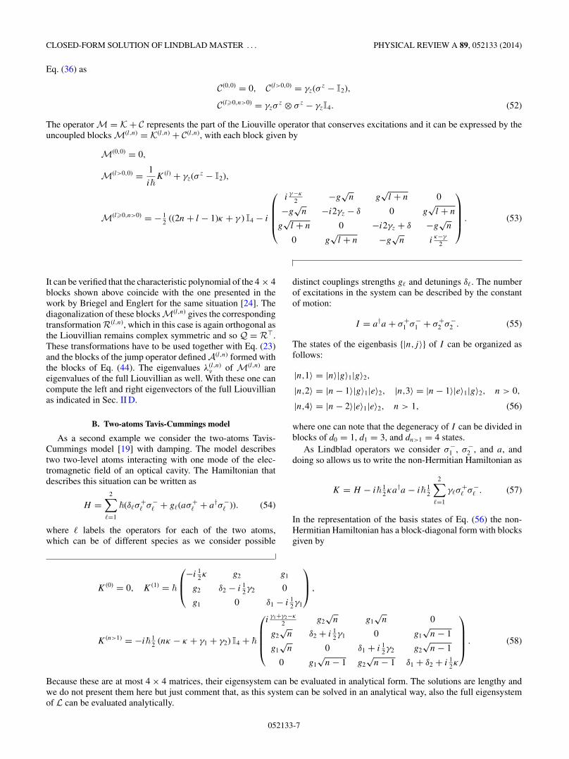
The operator M = K + C represents the part of the Liouville operator that conserves excitations and it can be expressed by theuncoupled blocks M(l,n) = K(l,n) + C(l,n), with each block given by

M(0,0) = 0,

M(l>0,0) = 1

i�K (l) + γz(σ

z − I2),

M(l�0,n>0) = − 12 ((2n + l − 1)κ + γ ) I4 − i

⎛⎜⎜⎜⎝

iγ−κ

2 −g√

n g√

l + n 0

−g√

n −i2γz − δ 0 g√

l + n

g√

l + n 0 −i2γz + δ −g√

n

0 g√

l + n −g√

n iκ−γ

2

⎞⎟⎟⎟⎠ . (53)

It can be verified that the characteristic polynomial of the 4 × 4blocks shown above coincide with the one presented in thework by Briegel and Englert for the same situation [24]. Thediagonalization of these blocks M(l,n) gives the correspondingtransformation R(l,n), which in this case is again orthogonal asthe Liouvillian remains complex symmetric and so Q = R.These transformations have to be used together with Eq. (23)and the blocks of the jump operator defined A(l,n) formed withthe blocks of Eq. (44). The eigenvalues λ(l,n)

ν of M(l,n) areeigenvalues of the full Liouvillian as well. With these one cancompute the left and right eigenvectors of the full Liouvillianas indicated in Sec. II D.

B. Two-atoms Tavis-Cummings model

As a second example we consider the two-atoms Tavis-Cummings model [19] with damping. The model describestwo two-level atoms interacting with one mode of the elec-tromagnetic field of an optical cavity. The Hamiltonian thatdescribes this situation can be written as

H =2∑

�=1

�(δ�σ+� σ−

� + g�(aσ+� + a†σ−

� )). (54)

where � labels the operators for each of the two atoms,which can be of different species as we consider possible

distinct couplings strengths g� and detunings δ�. The numberof excitations in the system can be described by the constantof motion:

I = a†a + σ+1 σ−

1 + σ+2 σ−

2 . (55)

The states of the eigenbasis {|n,j 〉} of I can be organized asfollows:

|n,1〉 = |n〉|g〉1|g〉2,

|n,2〉 = |n − 1〉|g〉1|e〉2, |n,3〉 = |n − 1〉|e〉1|g〉2, n > 0,

|n,4〉 = |n − 2〉|e〉1|e〉2, n > 1, (56)

where one can note that the degeneracy of I can be divided inblocks of d0 = 1, d1 = 3, and dn>1 = 4 states.

As Lindblad operators we consider σ−1 , σ−

2 , and a, anddoing so allows us to write the non-Hermitian Hamiltonian as

K = H − i� 12κa†a − i� 1

2

2∑�=1

γ�σ+� σ−

� . (57)

In the representation of the basis states of Eq. (56) the non-Hermitian Hamiltonian has a block-diagonal form with blocksgiven by

K (0) = 0, K (1) = �

⎛⎜⎝

−i 12κ g2 g1

g2 δ2 − i 12γ2 0

g1 0 δ1 − i 12γ1

⎞⎟⎠ ,

K (n>1) = −i� 12 (nκ − κ + γ1 + γ2) I4 + �

⎛⎜⎜⎜⎝

iγ1+γ2−κ

2 g2√

n g1√

n 0

g2√

n δ2 + i 12γ1 0 g1

√n − 1

g1√

n 0 δ1 + i 12γ2 g2

√n − 1

0 g1√

n − 1 g2√

n − 1 δ1 + δ2 + i 12κ

⎞⎟⎟⎟⎠ . (58)

Because these are at most 4 × 4 matrices, their eigensystem can be evaluated in analytical form. The solutions are lengthy andwe do not present them here but just comment that, as this system can be solved in an analytical way, also the full eigensystemof L can be evaluated analytically.

052133-7

JUAN MAURICIO TORRES PHYSICAL REVIEW A 89, 052133 (2014)

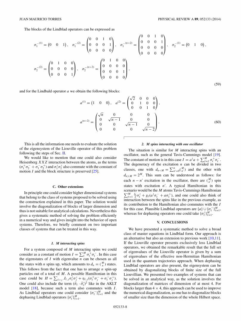
The blocks of the Lindblad operators can be expressed as

σ−1

(1) = (0 0 1

), σ−

1(2) =

⎛⎜⎝

0 0 1 0

0 0 0 1

0 0 0 0

⎞⎟⎠ , σ−

1(n>2) =

⎛⎜⎜⎜⎝

0 0 1 0

0 0 0 1

0 0 0 0

0 0 0 0

⎞⎟⎟⎟⎠ , σ−

2(1) = (

0 1 0),

σ−2

(2) =

⎛⎜⎝

0 1 0 0

0 0 0 0

0 0 0 1

⎞⎟⎠ , σ−

2(n>2) =

⎛⎜⎜⎜⎝

0 1 0 0

0 0 0 0

0 0 0 1

0 0 0 0

⎞⎟⎟⎟⎠ ,

(59)

and for the Lindbald operator a we obtain the following blocks:

a(1) = (1 0 0

), a(2) =

⎛⎝

√2 0 0 0

0 1 0 00 0 1 0

⎞⎠ ,

a(n>2) =

⎛⎜⎜⎝

√n 0 0 0

0√

n − 1 0 00 0

√n − 1 0

0 0 0√

n − 2

⎞⎟⎟⎠ . (60)

This is all the information one needs to evaluate the solutionof the eigensystem of the Liouville operator of this problemfollowing the steps of Sec. II.

We would like to mention that one could also considerHeisenberg XXZ interaction between the atoms, as the terms(σ+

1 σ−2 + σ−

1 σ+2 ) and σ z

1 σ z2 also commute with the constant of

motion I and the block structure is preserved [25].

C. Other extensions

In principle one could consider higher dimensional systemsthat belong to the class of systems proposed to be solved usingthe construction explained in this paper. The solution wouldinvolve the diagonalization of blocks of larger dimension andthus is not suitable for analytical calculations. Nevertheless thisgives a systematic method of solving the problem efficientlyin a numerical way and gives insight into the behavior of opensystems. Therefore, we briefly comment on two importantclasses of systems that can be treated in this way.

1. M interacting spins

For a system composed of M interacting spins we couldconsider as a constant of motion I = ∑M

� σ+� σ−

� . In this casethe eigenstates of I with eigenvalue n can be chosen as allthe states with n spins up, which amounts to dn = (M

n ) states.This follows from the fact that one has to arrange n spin-upparticles out of a total of M . A possible Hamiltonian in thiscase could be H = ∑

�>j J�,j σz� σ z

j + η�,j (σ+� σ−

j + σ−� σ+

j ).One could also include the term (�σ� · �σ ′

�)2 like in the AKLTmodel [18], because such a term also commutes with I .As Lindblad operators one could consider {σ−

� }M�=1 and thedephasing Lindblad operators {σ z

� }M�=1.

2. M spins interacting with one oscillator

The situation is similar for M interacting spins with anoscillator, such as the general Tavis-Cummings model [19].The constant of motion is in this case I = a†a + ∑M

�=1 σ+� σ−

� .The degeneracy of the excitation n can be divided in twoclasses, one with dn<M = ∑n

n′=0(Mn′ ) and the other with

dn�M = 2M . This sum can be understood as follows: foreach n − n′ excitation in the oscillator, there are (M

n′ ) spinstates with excitation n′. A typical Hamiltonian in thisscenario would be the M atoms Tavis-Cummings Hamiltonian∑M

�=1δ�

2 σ z� + g�(a†σ−

� + aσ+� ), and one could also think of

interaction between the spins like in the previous example, asits contribution to the Hamiltonian also commutes with the I

for this case. Plausible Lindblad operators are {a} ∪ {σ−� }M�=1,

whereas for dephasing operators one could take {σ z� }M�=1.

V. CONCLUSIONS

We have presented a systematic method to solve a broadclass of master equations in Lindblad form. Our approach isan alternative but also an extension to previous work [10,11].If the Liouville operator presents exclusively loss Lindbladoperators, we obtained the remarkable result that the full setof eigenvalues of the Liouville operator is given by a sumof eigenvalues of the effective non-Hermitian Hamiltonianused in the quantum trajectories approach. When dephasingLindblad operators are also present, the eigensystem can beobtained by diagonalizing blocks of finite size of the fullLiouvillian. We presented two examples of systems that canbe solved in an analytical way, as the solution involves thediagonalization of matrices of dimension of at most 4. Forblocks larger than 4 × 4, this approach can be used to improvethe numerical diagonalization, as one has to diagonalize blocksof smaller size than the dimension of the whole Hilbert space.

052133-8

CLOSED-FORM SOLUTION OF LINDBLAD MASTER . . . PHYSICAL REVIEW A 89, 052133 (2014)

We also show as an application the analytical evaluationof the spontaneous emission spectrum of an excited atom inan empty cavity. This shows that the introduced method canbe manageable to deal with analytical calculations. In thissense, it also offers the possibility to deal with other moregeneral classes of Liouvillians in a perturbative manner. Inparticular the extension to nonzero temperature baths comes tomind, as the Lindbladian term that accounts for the incoherentpumping or gain acts typically with a smaller strength. In thisway the eigensystem obtained with this construction mightbe used as a starting point to solve more general problemsusing perturbation theory such as the evaluation resonancefluorescence spectra [26,27] or the derivation of reducedmaster equations [6].

To conclude we would like to mention that these ideas couldbe also helpful in solving systems like the coupled oscillatorsthat describe optomechanical systems [28]. In this case thefree Hamiltonian of the optical mode serves also as a constantof motion and the Lindblad operators of the mechanical modeare of the dephasing type.

ACKNOWLEDGMENTS

The author would like to thank Tomaz Prosen, MarcBienert, Thomas H. Seligman, and J. Zsolt Bernad forenriching discussion and useful comments. Postdoctoral GrantNo. CONACyT-162781 and the hospitality of the Instituto deCiencias Fısicas, Universidad Nacional Autonoma de Mexicowith Project No. PAPIIT-IG101113 are also acknowledged.

[1] G. Lindblad, Commun. Math. Phys. 48, 119 (1976).[2] H. Carmichael, An Open Systems Approach to Quantum Optics,

Lecture Notes in Physics Monographs Vol. 18 (Springer, Berlin,1993).

[3] C. W. Gardiner and P. Zoller, Quantum Noise (Springer, Berlin,2004).

[4] A. Kossakowski, Rep. Math. Phys. 3, 247 (1972).[5] V. Gorini, A. Kossakowski, and E. C. G. Sudarshan, J. Math.

Phys. 17, 821 (1976).[6] J. I. Cirac, R. Blatt, P. Zoller, and W. D. Phillips, Phys. Rev. A

46, 2668 (1992).[7] B. Kraus, H. P. Buchler, S. Diehl, A. Kantian, A. Micheli, and

P. Zoller, Phys. Rev. A 78, 042307 (2008).[8] F. Verstraete, M. Wolf, and I. J. Cirac, Nat. Phys. 5, 633 (2009).[9] T. Prosen, Phys. Rev. Lett. 107, 137201 (2011).

[10] H.-J. Briegel and B.-G. Englert, Phys. Rev. A 47, 3311 (1993).[11] S. M. Barnett and S. Stenholm, J. Mod. Opt. 47, 2869 (2000).[12] B. Daeubler, H. Risken, and L. Schoendorff, Phys. Rev. A 46,

1654 (1992).[13] L.-M. Kuang, X. Chen, G.-H. Chen, and M.-L. Ge, Phys. Rev.

A 56, 3139 (1997).[14] A.-J. van Wonderen, Phys. Rev. A 56, 3116 (1997).[15] B.-G. Englert and G. Morigi, in Coherent Evolution in Noisy

Environments, Lecture Notes in Physics Vol. 611, edited byA. Buchleitner and K. Hornberger (Springer, Berlin, 2002),pp. 55–106.

[16] M. B. Plenio and P. L. Knight, Rev. Mod. Phys. 70, 101(1998).

[17] A. Klumper, Z. Phys. B 91, 507 (1993).[18] I. Affleck, T. Kennedy, E. H. Lieb, and H. Tasaki, Phys. Rev.

Lett. 59, 799 (1987).[19] M. Tavis and F. W. Cummings, Phys. Rev. 170, 379

(1968).[20] E. Jaynes and F. Cummings, Proc. IEEE 51, 89 (1963).[21] If H is real, then K is complex symmetric and Q† = RT .[22] H. J. Carmichael, R. J. Brecha, M. G. Raizen, H. J. Kimble, and

P. R. Rice, Phys. Rev. A 40, 5516 (1989).[23] A. Auffeves, B. Besga, J.-M. Gerard, and J.-P. Poizat, Phys. Rev.

A 77, 063833 (2008).[24] See Eq. (4.7) in [10]. There is a misprint in Eq. (4.7a) of [10].

In the linear coefficient in �′ one has to replace 4g2 by 2g2. Thecharacteristic polynomial is obtained from the 4 × 4 matrix inEq. (3.6a) for ν = s = 0.

[25] J. M. Torres, E. Sadurnı, and T. H. Seligman, J. Phys. A 43,192002 (2010).

[26] M. Bienert, J. M. Torres, S. Zippilli, and G. Morigi, Phys. Rev.A 76, 013410 (2007).

[27] J. M. Torres, M. Bienert, S. Zippilli, and G. Morigi, Eur. Phys.J. D 61, 21 (2011).

[28] I. Wilson-Rae, N. Nooshi, J. Dobrindt, T. J.Kippenberg, and W. Zwerger, New J. Phys. 10, 095007(2008).

052133-9