CloudScale: Elastic Resource Scaling for Multi-Tenant

CloudScale: Elastic Resource Scaling forMulti-Tenant Cloud Systems

Zhiming Shen, Sethuraman Subbiah, Xiaohui Gu,Department of Computer Science

North Carolina State University{zshen5,ssubbia2}@ncsu.edu, [email protected]

John WilkesGoogle

Mountain View, [email protected]

ABSTRACT

Elastic resource scaling lets cloud systems meet application servicelevel objectives (SLOs) with minimum resource provisioning costs.In this paper, we present CloudScale, a system that automates fine-grained elastic resource scaling for multi-tenant cloud computinginfrastructures. CloudScale employs online resource demand pre-diction and prediction error handling to achieve adaptive resourceallocation without assuming any prior knowledge about the appli-cations running inside the cloud. CloudScale can resolve scalingconflicts between applications using migration, and integrates dy-namic CPU voltage/frequency scaling to achieve energy savingswith minimal effect on application SLOs. We have implementedCloudScale on top of Xen and conducted extensive experimentsusing a set of CPU and memory intensive applications (RUBiS,Hadoop, IBM System S). The results show that CloudScale canachieve significantly higher SLO conformance than other alterna-tives with low resource and energy cost. CloudScale is non-intrusiveand light-weight, and imposes negligible overhead (< 2% CPU inDomain 0) to the virtualized computing cluster.

Categories and Subject Descriptors

D.4.8 [Operating Systems]: Performance—Modeling and predic-

tion, Monitors; C.4 [Performance of Systems]: Modeling tech-niques

General Terms

Measurement, Performance

Keywords

Cloud Computing, Resource Scaling, Energy-efficient Computing

1. INTRODUCTIONMost Infrastructure as a Service (IaaS) providers [1, 6] use vir-

tualization technologies [10, 7, 3] to encapsulate applications and

Permission to make digital or hard copies of all or part of this work forpersonal or classroom use is granted without fee provided that copies arenot made or distributed for profit or commercial advantage and that copiesbear this notice and the full citation on the first page. To copy otherwise, torepublish, to post on servers or to redistribute to lists, requires prior specificpermission and/or a fee.SOCC’11, October 27–28, 2011, Cascais, Portugal.Copyright 2011 ACM 978-1-4503-0976-9/11/10 ...$10.00.

0 8 16 24 32 400

50

100

Under-estimation error

correction

Padding

Conflict

Under-estimation error

Res

ou

rce

(%)

Time (s)

Demand

Prediction

Cap

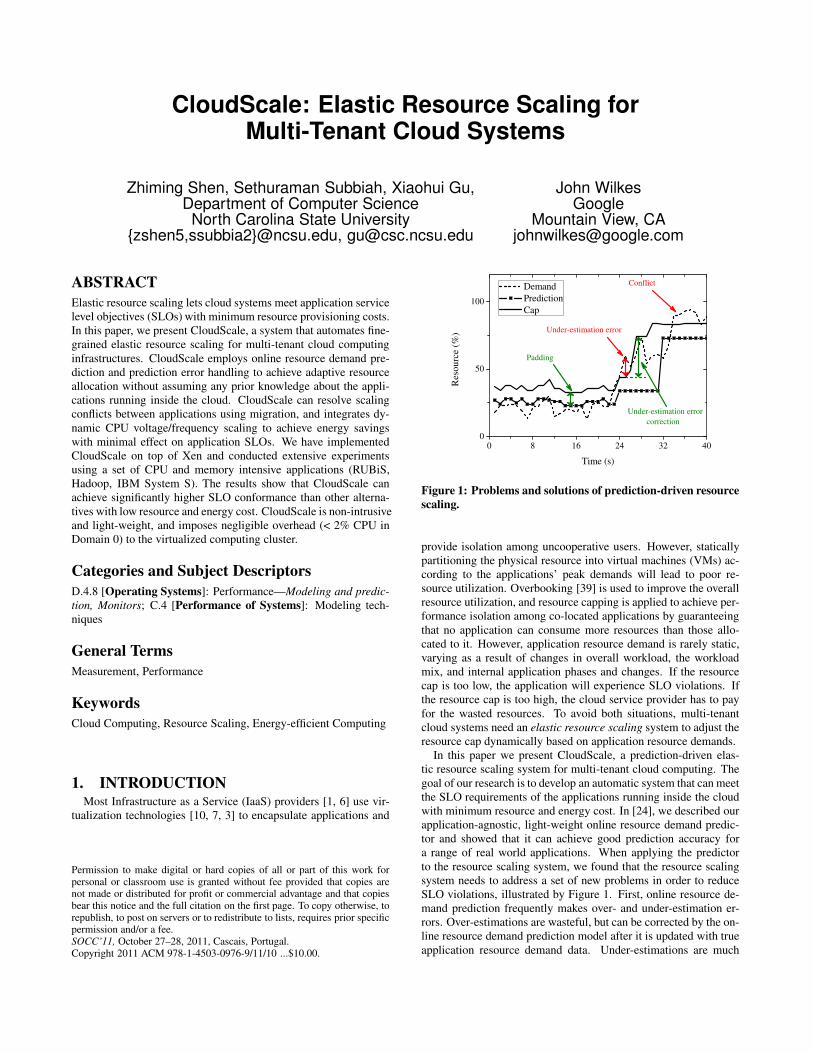
Figure 1: Problems and solutions of prediction-driven resource

scaling.

provide isolation among uncooperative users. However, staticallypartitioning the physical resource into virtual machines (VMs) ac-cording to the applications’ peak demands will lead to poor re-source utilization. Overbooking [39] is used to improve the overallresource utilization, and resource capping is applied to achieve per-formance isolation among co-located applications by guaranteeingthat no application can consume more resources than those allo-cated to it. However, application resource demand is rarely static,varying as a result of changes in overall workload, the workloadmix, and internal application phases and changes. If the resourcecap is too low, the application will experience SLO violations. Ifthe resource cap is too high, the cloud service provider has to payfor the wasted resources. To avoid both situations, multi-tenantcloud systems need an elastic resource scaling system to adjust theresource cap dynamically based on application resource demands.

In this paper we present CloudScale, a prediction-driven elas-tic resource scaling system for multi-tenant cloud computing. Thegoal of our research is to develop an automatic system that can meetthe SLO requirements of the applications running inside the cloudwith minimum resource and energy cost. In [24], we described ourapplication-agnostic, light-weight online resource demand predic-tor and showed that it can achieve good prediction accuracy fora range of real world applications. When applying the predictorto the resource scaling system, we found that the resource scalingsystem needs to address a set of new problems in order to reduceSLO violations, illustrated by Figure 1. First, online resource de-mand prediction frequently makes over- and under-estimation er-rors. Over-estimations are wasteful, but can be corrected by the on-line resource demand prediction model after it is updated with trueapplication resource demand data. Under-estimations are much

worse since they prevent the system from knowing the true appli-cation resource demand and may cause significant SLO violations.Second, co-located applications will conflict when the available re-sources are insufficient to accommodate all scale-up requirements.

CloudScale provides two complementary under-estimation errorhandling schemes: 1) online adaptive padding and 2) reactive errorcorrection. Our approach is based on the observation that reac-tive error correction alone is often insufficient. When an under-estimation error is detected, an SLO violation has probably alreadyhappened. Moreover, there is some delay before the scaling sys-tem can figure out the right resource cap. Thus, it is worthwhile toperform proactive padding to avoid under-estimation errors.

When a scaling conflict happens, we can either reject some scale-up requirements or migrate some applications [14] out of the over-loaded host. Migration is often disruptive, so if the conflict is tran-sient, it is not cost-effective to do this. Moreover, it is often toolate to trigger the migration on a conflict since the migration mighttake a long time to finish when the host is already overloaded. Ourapproach achieves predictive migration, which can start the migra-tion before the conflict happens to minimize the impact of migra-tion to both migrated and non-migrating applications. CloudScaleuses conflict prediction and resolution inference to decide whethera migration should be triggered, which application(s) should be mi-grated, and when the migration should be triggered.

We make the following contributions in this paper:

• We introduce a set of intelligent schemes to reduce SLO vi-olations in a prediction-driven resource scaling system.

• We show how using both adaptive padding and fast under-estimation error correction minimizes the impact of under-estimation errors with low resource waste.

• We evaluate how well predictive migration resolves scalingconflicts with minimum SLO impact.

• We demonstrate how combining resource scaling with CPUvoltage and frequency scaling can save energy without af-fecting application SLOs.

The rest of the paper is organized as follows. Section 2 presentsthe system design of CloudScale. Section 3 presents the experi-mental results. Section 4 compares our work with related work.Section 5 discusses the limitations and future work. Finally, thepaper concludes in Section 6.

2. CLOUDSCALE DESIGNIn this section, we present the design of CloudScale. First, we

provide an overview of our approach. Then, we introduce the sin-gle VM scaling algorithms that can efficiently handle runtime pre-diction errors. Next, we describe how to resolve scaling conflicts.Finally, we describe the integrated VM resource scaling and CPUfrequency and voltage scaling for energy saving.

2.1 OverviewCloudScale runs within each host in the cloud system, and is

complementary to the resource allocation scheme that handles coarse-grained replicated server capacity scaling [30, 38, 9]. CloudScaleis built on top of the Xen virtualization platform. Figure 2 showsthe overall architecture of the CloudScale System.

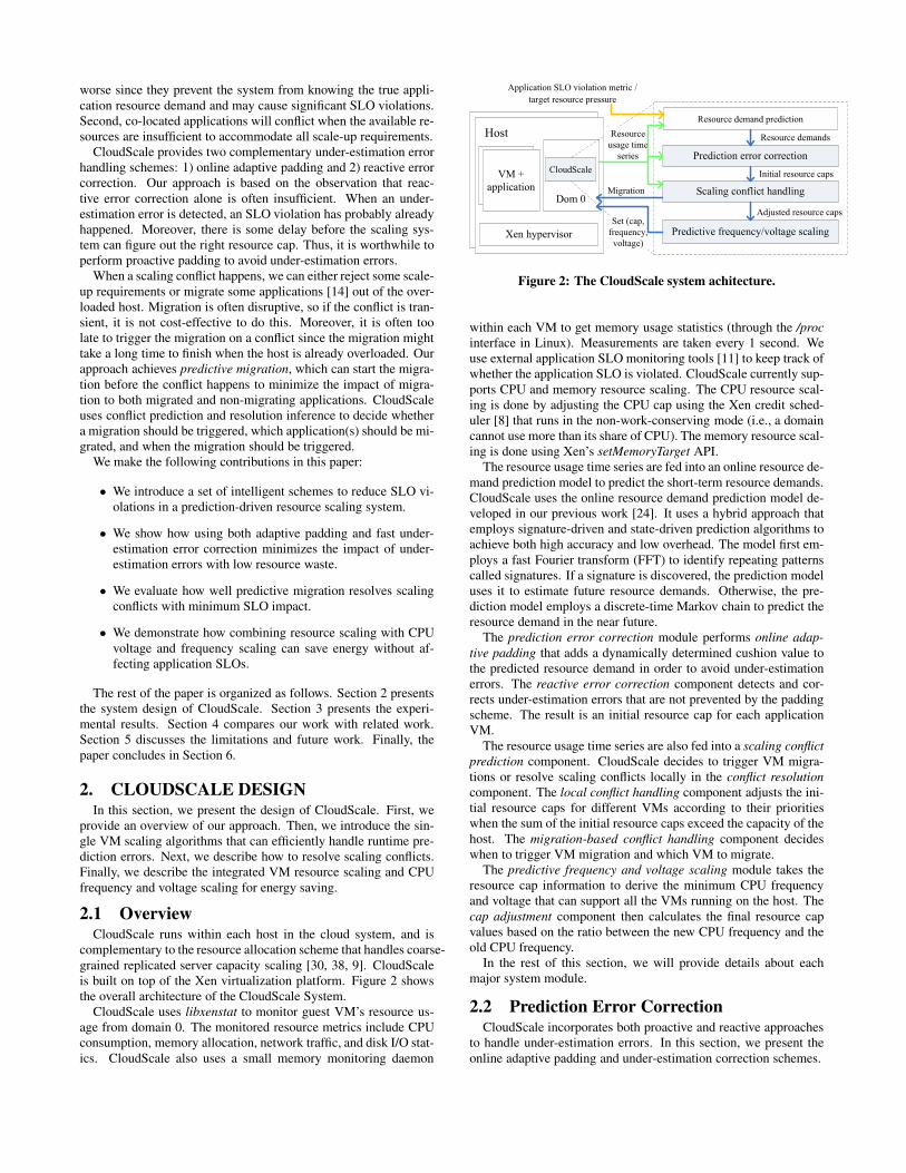
CloudScale uses libxenstat to monitor guest VM’s resource us-age from domain 0. The monitored resource metrics include CPUconsumption, memory allocation, network traffic, and disk I/O stat-ics. CloudScale also uses a small memory monitoring daemon

Figure 2: The CloudScale system achitecture.

within each VM to get memory usage statistics (through the /proc

interface in Linux). Measurements are taken every 1 second. Weuse external application SLO monitoring tools [11] to keep track ofwhether the application SLO is violated. CloudScale currently sup-ports CPU and memory resource scaling. The CPU resource scal-ing is done by adjusting the CPU cap using the Xen credit sched-uler [8] that runs in the non-work-conserving mode (i.e., a domaincannot use more than its share of CPU). The memory resource scal-ing is done using Xen’s setMemoryTarget API.

The resource usage time series are fed into an online resource de-mand prediction model to predict the short-term resource demands.CloudScale uses the online resource demand prediction model de-veloped in our previous work [24]. It uses a hybrid approach thatemploys signature-driven and state-driven prediction algorithms toachieve both high accuracy and low overhead. The model first em-ploys a fast Fourier transform (FFT) to identify repeating patternscalled signatures. If a signature is discovered, the prediction modeluses it to estimate future resource demands. Otherwise, the pre-diction model employs a discrete-time Markov chain to predict theresource demand in the near future.

The prediction error correction module performs online adap-

tive padding that adds a dynamically determined cushion value tothe predicted resource demand in order to avoid under-estimationerrors. The reactive error correction component detects and cor-rects under-estimation errors that are not prevented by the paddingscheme. The result is an initial resource cap for each applicationVM.

The resource usage time series are also fed into a scaling conflict

prediction component. CloudScale decides to trigger VM migra-tions or resolve scaling conflicts locally in the conflict resolution

component. The local conflict handling component adjusts the ini-tial resource caps for different VMs according to their prioritieswhen the sum of the initial resource caps exceed the capacity of thehost. The migration-based conflict handling component decideswhen to trigger VM migration and which VM to migrate.

The predictive frequency and voltage scaling module takes theresource cap information to derive the minimum CPU frequencyand voltage that can support all the VMs running on the host. Thecap adjustment component then calculates the final resource capvalues based on the ratio between the new CPU frequency and theold CPU frequency.

In the rest of this section, we will provide details about eachmajor system module.

2.2 Prediction Error CorrectionCloudScale incorporates both proactive and reactive approaches

to handle under-estimation errors. In this section, we present theonline adaptive padding and under-estimation correction schemes.

0 100 200 300 4000

20

40

60

80

100

CP

U u

sag

e (%

)

Time (s)

Original time series

Padding values

Extracted burst pattern

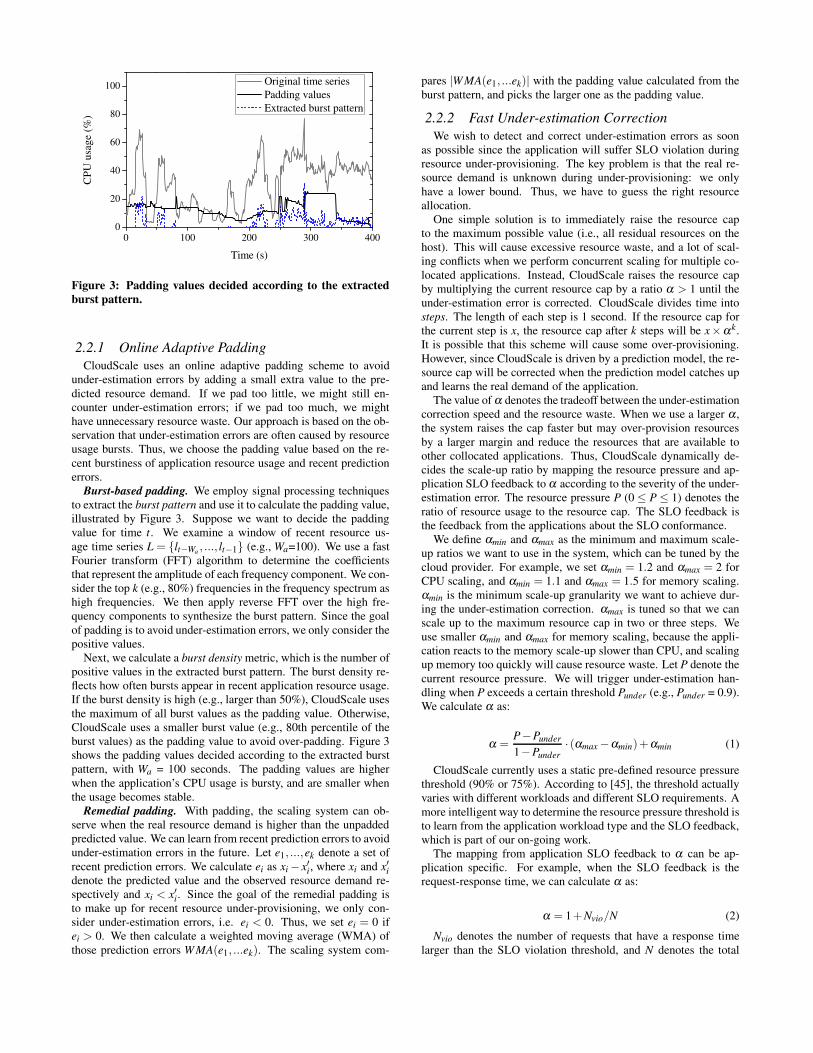
Figure 3: Padding values decided according to the extracted

burst pattern.

2.2.1 Online Adaptive Padding

CloudScale uses an online adaptive padding scheme to avoidunder-estimation errors by adding a small extra value to the pre-dicted resource demand. If we pad too little, we might still en-counter under-estimation errors; if we pad too much, we mighthave unnecessary resource waste. Our approach is based on the ob-servation that under-estimation errors are often caused by resourceusage bursts. Thus, we choose the padding value based on the re-cent burstiness of application resource usage and recent predictionerrors.

Burst-based padding. We employ signal processing techniquesto extract the burst pattern and use it to calculate the padding value,illustrated by Figure 3. Suppose we want to decide the paddingvalue for time t. We examine a window of recent resource us-age time series L = {lt−Wa

, ..., lt−1} (e.g., Wa=100). We use a fastFourier transform (FFT) algorithm to determine the coefficientsthat represent the amplitude of each frequency component. We con-sider the top k (e.g., 80%) frequencies in the frequency spectrum ashigh frequencies. We then apply reverse FFT over the high fre-quency components to synthesize the burst pattern. Since the goalof padding is to avoid under-estimation errors, we only consider thepositive values.

Next, we calculate a burst density metric, which is the number ofpositive values in the extracted burst pattern. The burst density re-flects how often bursts appear in recent application resource usage.If the burst density is high (e.g., larger than 50%), CloudScale usesthe maximum of all burst values as the padding value. Otherwise,CloudScale uses a smaller burst value (e.g., 80th percentile of theburst values) as the padding value to avoid over-padding. Figure 3shows the padding values decided according to the extracted burstpattern, with Wa = 100 seconds. The padding values are higherwhen the application’s CPU usage is bursty, and are smaller whenthe usage becomes stable.

Remedial padding. With padding, the scaling system can ob-serve when the real resource demand is higher than the unpaddedpredicted value. We can learn from recent prediction errors to avoidunder-estimation errors in the future. Let e1, ...,ek denote a set ofrecent prediction errors. We calculate ei as xi − x′i, where xi and x′idenote the predicted value and the observed resource demand re-spectively and xi < x′i. Since the goal of the remedial padding isto make up for recent resource under-provisioning, we only con-sider under-estimation errors, i.e. ei < 0. Thus, we set ei = 0 ifei > 0. We then calculate a weighted moving average (WMA) ofthose prediction errors W MA(e1, ...ek). The scaling system com-

pares |W MA(e1, ...ek)| with the padding value calculated from theburst pattern, and picks the larger one as the padding value.

2.2.2 Fast Under-estimation Correction

We wish to detect and correct under-estimation errors as soonas possible since the application will suffer SLO violation duringresource under-provisioning. The key problem is that the real re-source demand is unknown during under-provisioning: we onlyhave a lower bound. Thus, we have to guess the right resourceallocation.

One simple solution is to immediately raise the resource capto the maximum possible value (i.e., all residual resources on thehost). This will cause excessive resource waste, and a lot of scal-ing conflicts when we perform concurrent scaling for multiple co-located applications. Instead, CloudScale raises the resource capby multiplying the current resource cap by a ratio α > 1 until theunder-estimation error is corrected. CloudScale divides time intosteps. The length of each step is 1 second. If the resource cap forthe current step is x, the resource cap after k steps will be x×αk.It is possible that this scheme will cause some over-provisioning.However, since CloudScale is driven by a prediction model, the re-source cap will be corrected when the prediction model catches upand learns the real demand of the application.

The value of α denotes the tradeoff between the under-estimationcorrection speed and the resource waste. When we use a larger α ,the system raises the cap faster but may over-provision resourcesby a larger margin and reduce the resources that are available toother collocated applications. Thus, CloudScale dynamically de-cides the scale-up ratio by mapping the resource pressure and ap-plication SLO feedback to α according to the severity of the under-estimation error. The resource pressure P (0 ≤ P ≤ 1) denotes theratio of resource usage to the resource cap. The SLO feedback isthe feedback from the applications about the SLO conformance.

We define αmin and αmax as the minimum and maximum scale-up ratios we want to use in the system, which can be tuned by thecloud provider. For example, we set αmin = 1.2 and αmax = 2 forCPU scaling, and αmin = 1.1 and αmax = 1.5 for memory scaling.αmin is the minimum scale-up granularity we want to achieve dur-ing the under-estimation correction. αmax is tuned so that we canscale up to the maximum resource cap in two or three steps. Weuse smaller αmin and αmax for memory scaling, because the appli-cation reacts to the memory scale-up slower than CPU, and scalingup memory too quickly will cause resource waste. Let P denote thecurrent resource pressure. We will trigger under-estimation han-dling when P exceeds a certain threshold Punder (e.g., Punder = 0.9).We calculate α as:

α =P−Punder

1−Punder

· (αmax −αmin)+αmin (1)

CloudScale currently uses a static pre-defined resource pressurethreshold (90% or 75%). According to [45], the threshold actuallyvaries with different workloads and different SLO requirements. Amore intelligent way to determine the resource pressure threshold isto learn from the application workload type and the SLO feedback,which is part of our on-going work.

The mapping from application SLO feedback to α can be ap-plication specific. For example, when the SLO feedback is therequest-response time, we can calculate α as:

α = 1+Nvio/N (2)

Nvio denotes the number of requests that have a response timelarger than the SLO violation threshold, and N denotes the total

number of requests during the previous sampling period (e.g., 1second). For Hadoop applications, the SLO feedback can be jobprogress scores. We calculate α as 1+(Pre f −P)/Pre f , where Pre f

denotes the desired progress score derived from the target comple-tion time of the job, and P denotes the current progress score.

When both resource pressure and SLO feedback are available,CloudScale chooses the larger one as the final α .

2.3 Scaling Conflict HandlingIn this section, we describe how we handle concurrent resource

scaling for multiple co-located applications. The key issue is todeal with scaling conflicts when the available resources are insuffi-cient to accommodate all scale-up requirements on a host. We firstdescribe how to predict the conflict. Then we introduce the localconflict handling and migration-based conflict handling schemes.Finally we describe the policy of choosing different conflict han-dling approaches.

2.3.1 Conflict Prediction

We can resolve a scaling conflict by either rejecting some ap-plications’ scale-up requirements or employing VM migration tomitigate the conflict. Both approaches will probably cause SLO vi-olations, but we try to minimize these. We use a conflict predictionmodel to estimate 1) when the conflict will happen, 2) how seriousthe conflict will be, and 3) how long the conflict will last.

We leverage our resource demand prediction schemes for con-flict prediction, looking further into the future. The scaling systemmaintains a long-term resource demand prediction model for eachVM. Different with the prediction model used by the resource scal-ing system, which uses 1-second prediction interval, the long-termprediction model uses 10-second prediction interval in order to pre-dict further into the future. We use Wb to denote the length of thelook-ahead window of the long-term prediction model (e.g., Wb =100 seconds). Suppose a host runs K application VMs: m1,...,mK.Let {ri,t+1, ...ri,t+Wb

} denote predicted future resource demands onthe mi from time t + 1 to t +Wb. We can then derive the total re-

source demand time series on the host as {K

∑i=1

ri,t+1, ...K

∑i=1

ri,t+Wb}.

By comparing this total resource demand time series with the hostresource capacity C, we can estimate when a conflict will happen

(i.e.,K

∑i=1

ri,t1 >C, t1 denotes the conflict start time), how serious the

conflict will be (i.e., the conflict degree:K

∑i=1

ri,t1 −C), and how long

the conflict will last.

2.3.2 Local conflict handling

If the conflict duration is short and the conflict degree is small,we resolve the scaling conflict locally without invoking expensivemigration operations. We define SLO penalty as the financial lossfor the cloud provider when applications experience SLO viola-tions, and we use RPi (Resource under-provisioning Penalty) to de-note the SLO penalty for the application VM mi caused by one unitresource under-provisioning.

Using local conflict handling, we need to consider how to dis-tribute the resource under-provisioning impact among different ap-plications. CloudScale supports both uniform and differentiatedlocal conflict handling. In the uniform scheme, we set the resourcecap for each application in proportion to its resource demand. Sup-pose the predicted resource demand for the application VM mi is

ri. We set the resource cap for mi as (ri/K

∑i=1

ri) ·C, where C de-

notes the total resource capacity on the host. In the differentiated

scheme, CloudScale allocates resources based on application pri-orities or resource under-provisioning penalties (RPi) of differentapplications in order to minimize the total penalty. For example,when the VMs have different priorities, CloudScale strives first tosatisfy the resource requirements of high-priority applications andonly share the under-provisioning impact among low priority appli-cations. CloudScale first ranks all applications according to theirpriorities, and decides the resource caps of different applicationsbased on the priority rank. If the application’s resource demandcan be satisfied by the residual resource, CloudScale will allocatethe required resource to the application. Otherwise, CloudScale al-locates the residual resources to all the remaining applications inproportion to their resource demands. We can apply a similar dif-ferentiated allocation scheme when RPi is used to rank differentapplications.

We estimate the total SLO penalty for mi based on the conflict

prediction results ast2

∑k=t1

RPi ·ei,t+k, where t1 and t2 denote the con-

flict start and end time, and ei,t+k denotes the under-estimation er-ror at time t +k. We aggregate the SLO penalties of all applicationVMs to calculate the total resource under-provisioning penalty QRP

using the local conflict handling scheme.

2.3.3 Migration-based conflict handling

If we decide to resolve the scaling conflict using VM migra-tion, we first need to decide when to trigger the migration. Weobserve that Xen live migration is CPU intensive. Without properisolation, the migration will cause significant SLO impact to bothmigrated and non-migrating applications on both source and des-tination hosts. Furthermore, without sufficient CPU, the migrationwill take a long time to finish, which will lead to a long servicedegradation time. It is often too late to trigger the migration afterthe conflict already happened and the host is already overloaded.To address the problem, we use predictive migration, which lever-ages the conflict prediction to trigger migration before the conflicthappens. If we want to trigger migration I (e.g., I = 70s) beforethe conflict happens, the migration-based conflict handling mod-ule will check whether any conflict that needs to be resolved usingmigration will happen after time t + I, where t denotes the currenttime. If positive, the module will trigger the migration now at timet rather than wait until the conflict happens later after time t + I.

To avoid triggering unnecessary migrations for mis-predicted ortransient conflicts, the migration will be triggered only if the con-flict is predicted to last continuously for at least K seconds. Thevalue of K denotes the tradeoff between correct predictions andfalse alarms, and can be tuned by the cloud provider. Typically weset K = 30s, which corresponds to three consecutive predicted con-flicts using a 10-second prediction interval. As a future work, wewill make K a function of the migration lead time I and the VMmigration time. We may use larger K for longer migration leadtime since it will be more likely to have false alarms given a longermigration lead time. For VMs that have longer migration time, wewant to avoid unnecessary migrations by using a larger K for lowerfalse alarm rate.

Next, we need to decide which application VMs should be mi-grated. Since modern data centers usually have high speed net-works, the network cost for migration typically is not the majorconcern. Instead, our scheme focuses on i) migrating as few VMsas possible, and 2) minimizing SLO penalty caused by migrations.Similar to previous work [41], we consider a normalized SLO penaltymetric: Zi =MPi ·Ti/(w1 ·cpui+w2 ·memi), where MPi (MigrationPenalty) denotes the unit SLO penalty for the application VM mi

during the migration1; Ti denotes the total migration time for mi;cpui and memi denote the normalized CPU and memory utilizationof the application VM mi compared to the capacity of the host. Theweights w1 and w2 denote the importance of the CPU resource orthe memory resource in our decision-making. We can give a higherweight to the bottleneck resource that has lower availability. Forexample, if the host is CPU-overloaded but has plentiful memory,w1 can be much larger than w2 so that we will choose a VM withhigh CPU consumptions to release sufficient CPU resource. In-tuitively, if the application has low SLO penalty during migrationand high resource demands, we want to migrate this applicationfirst since the migration imposes low SLO penalty to the migratedapplication and can release a large amount of resources to resolveconflicts. We sort all application VMs using the normalized SLOpenalty metric, and start to migrate the application VMs from theone with the smallest SLO penalty until sufficient resources are re-leased to resolve the conflicts.

Finally, we need to decide which host the selected VM should bemigrated to. CloudScale relies on a centralized controller to selectthe destination host for the migrated application. For example, wecan use a greedy algorithm to migrate the VMs to the least loadedhost that can accommodate the VM [41], or we can find a suitablehost by matching the resource demand signature of the VM withthe residual resource signature of the host [23].

We calculate the SLO penalty for migrating mi as MPi · Ti. Inour current implementation, we estimate the migration time usinga linear function of average memory footprint. The function is de-rived from a few measurement samples using linear regression. Wecan then aggregate the SLO penalties of all migrated VMs to derivethe total migration penalty QM using the migration-based conflicthandling scheme.

2.3.4 Conflict Resolution Inference

CloudScale currently decides whether to trigger migration bycomparing QRP and QM . If QRP ≥ QM , CloudScale will not mi-grate any application VM and resolve the scaling conflict using thelocal conflict handling scheme. Otherwise, CloudScale migratesselected VMs out until sufficient resources are released to resolvethe conflict. As a future work, we can also adopt a hybrid ap-proach that combines both local conflict handling and migration-based conflict handling to minimize the total SLO penalty QRP +QM . We can estimate the total SLO penalty QRP +QM of migrat-ing different subsets of VMs, and choose the migrated subset thatminimizes the total SLO penalty.

The unit SLO penalty values RPi and MPi are application de-pendent. We assume that these are provided to CloudScale bythe user. Typically, batch processing applications (e.g., long run-ning MapReduce jobs) are more tolerant of short periods of ser-vice degradation than time-sensitive interactive applications suchas Web transactions.

2.4 Predictive Frequency/Voltage ScalingCloudScale integrates VM resource scaling with dynamic volt-

age and frequency scaling (DVFS) to transform unused resourcesinto energy savings without affecting application SLOs. For ex-ample, if the resource demand prediction models indicate that thetotal CPU resource demand on a host is 50%, we can then halfthe CPU frequency and double the resource caps of all applicationVMs. Thus, we can reduce energy consumption since the CPU runsat a slower speed but the application’s SLO is unaffected. Another

1Although Xen live migration shortens the VM downtime, the ap-plication may experience a period of high SLO violations due tothe memory copy.

way of saving energy is to let the application run as fast as possibleand then shutdown the machine. However, the host in the multi-tenant cloud system often runs some interactive foreground jobsthat are expected to operate 24x7. Thus, we believe that slowingdown the CPU is a more practical solution in this case.

Modern processors often can run at a range of frequencies andvoltages and support dynamic frequency/voltage scaling. Supposethe host processor can operate at k different frequencies: f1 < ... <fk and the current frequency is fi. For example, the processor in ourexperimental testbed supports 11 different frequencies. We want toslow down the CPU based on the current resource cap informationto ensure that application performance is not affected. Let C′ andC denote the total CPU demand by all the application VMs andthe CPU capacity of the host, respectively. We can then derivethe current CPU utilization as C′/C. If the current host does nothave a full utilization (i.e., C′/C < 1) and the current frequencyfi is not the lowest, CloudScale picks the lowest frequency f j thatmeets the condition: f j ≥ C′/C · fi. If f j < fi, we scale down theCPU frequency to f j. We then multiply the resource caps for allapplication VMs by fi/ f j to maintain the application SLOs. Tomaintain the accuracy of the resource demand prediction, we alsoneed to scale up the stored resource demand training data by fi/ f j

to match the new CPU frequency.If the processor is not running at the highest frequency, we can

increase the CPU speed to try to resolve scaling conflicts. For ex-ample, if the future CPU demand is predicted to be C′,C′ >C andthe current frequency is fi, we will scale up the CPU frequency tothe slowest one f j among fi+1, ... fk such that f j/ fi >C′/C. Afterwe set the CPU frequency to f j, we will scale down the resourcecap ri for each application VM to ri · ( fi/ f j) to match the new CPUfrequency. After we reach the highest frequency, we will resort toeither local conflict handling or migration-based conflict handling,as described in the previous section.

3. EXPERIMENTAL EVALUATIONWe implemented CloudScale on top of the Xen virtualization

platform and conducted extensive evaluation studies using the RU-BiS [4] online auction benchmark (PhP version), Hadoop MapRe-duce systems [2, 15], and IBM System S data stream processingsystem [21]. This section describes our results.

3.1 Experiment setupMost of our experiments were conducted in the NCSU’s Virtual

Computing Lab (VCL) [6]. Each VCL host has a dual-core Xeon3.00GHz CPU, 4GB memory and 100Mbps network bandwidth,and runs CentOS 5.2 64bit with Xen 3.0.3. The guest VMs alsorun CentOS 5.2 64bit and have one virtual CPU core (the small-est scheduling unit in Xen hypervisor, similar to the task in Linuxkernel).

The integrated VM scaling and DVFS experiments were con-ducted on the Hybrid Green Cloud Computing (HGCC) cluster inour department since VCL hosts are not equipped with power me-ters. Each HGCC node has a quad-core Xeon 2.53GHz processor,8GB memory and 1Gbps network bandwidth, and runs CentOS 5.564 bit with Xen 3.4.3. The processor supports 11 frequency stepsbetween 2.53 and 1.19Ghz. We used Watts Up power meters to getreal time power readings from HGCC hosts. The guest VM OS isthe same with the VCL host. We use Intel SpeedStep technology toperform DVFS. We run our systems on DVFS enabled Linux 2.6.18kernel and control the CPU frequency from the host OS using theLinux CPUfreq subsystem.

In all of our experiments, we pin down Domain 0 to one core and

0 1 2 3 4 5 60

20

40

60

80

100 EPA

Time (hours)

0 1 2 3 4 5 60

20

40

60

80

100 Word Cup

CP

U u

sag

e (%

)

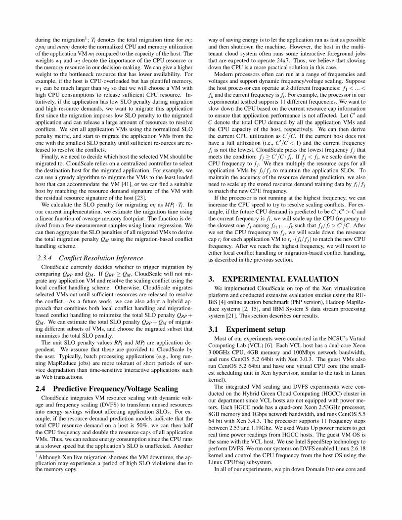
Figure 4: The real uncapped CPU demand of the RUBiS web-

server under two different workloads.

-30 -20 -10 0 10 20 300

10

20

30

40

50

Cu

mu

lati

ve P

erc

en

tag

e (

%)

CPU prediction error (%)

World Cup

EPA

100

90

80

70

60

50

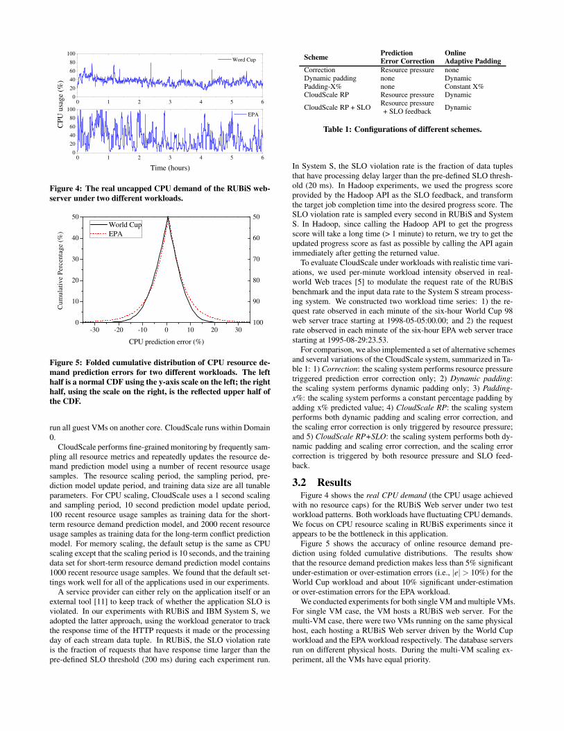
Figure 5: Folded cumulative distribution of CPU resource de-

mand prediction errors for two different workloads. The left

half is a normal CDF using the y-axis scale on the left; the right

half, using the scale on the right, is the reflected upper half of

the CDF.

run all guest VMs on another core. CloudScale runs within Domain0.

CloudScale performs fine-grained monitoring by frequently sam-pling all resource metrics and repeatedly updates the resource de-mand prediction model using a number of recent resource usagesamples. The resource scaling period, the sampling period, pre-diction model update period, and training data size are all tunableparameters. For CPU scaling, CloudScale uses a 1 second scalingand sampling period, 10 second prediction model update period,100 recent resource usage samples as training data for the short-term resource demand prediction model, and 2000 recent resourceusage samples as training data for the long-term conflict predictionmodel. For memory scaling, the default setup is the same as CPUscaling except that the scaling period is 10 seconds, and the trainingdata set for short-term resource demand prediction model contains1000 recent resource usage samples. We found that the default set-tings work well for all of the applications used in our experiments.

A service provider can either rely on the application itself or anexternal tool [11] to keep track of whether the application SLO isviolated. In our experiments with RUBiS and IBM System S, weadopted the latter approach, using the workload generator to trackthe response time of the HTTP requests it made or the processingday of each stream data tuple. In RUBiS, the SLO violation rateis the fraction of requests that have response time larger than thepre-defined SLO threshold (200 ms) during each experiment run.

SchemePredictionError Correction

OnlineAdaptive Padding

Correction Resource pressure noneDynamic padding none DynamicPadding-X% none Constant X%CloudScale RP Resource pressure Dynamic

CloudScale RP + SLOResource pressure+ SLO feedback

Dynamic

Table 1: Configurations of different schemes.

In System S, the SLO violation rate is the fraction of data tuplesthat have processing delay larger than the pre-defined SLO thresh-old (20 ms). In Hadoop experiments, we used the progress scoreprovided by the Hadoop API as the SLO feedback, and transformthe target job completion time into the desired progress score. TheSLO violation rate is sampled every second in RUBiS and SystemS. In Hadoop, since calling the Hadoop API to get the progressscore will take a long time (> 1 minute) to return, we try to get theupdated progress score as fast as possible by calling the API againimmediately after getting the returned value.

To evaluate CloudScale under workloads with realistic time vari-ations, we used per-minute workload intensity observed in real-world Web traces [5] to modulate the request rate of the RUBiSbenchmark and the input data rate to the System S stream process-ing system. We constructed two workload time series: 1) the re-quest rate observed in each minute of the six-hour World Cup 98web server trace starting at 1998-05-05:00.00; and 2) the requestrate observed in each minute of the six-hour EPA web server tracestarting at 1995-08-29:23.53.

For comparison, we also implemented a set of alternative schemesand several variations of the CloudScale system, summarized in Ta-ble 1: 1) Correction: the scaling system performs resource pressuretriggered prediction error correction only; 2) Dynamic padding:the scaling system performs dynamic padding only; 3) Padding-

x%: the scaling system performs a constant percentage padding byadding x% predicted value; 4) CloudScale RP: the scaling systemperforms both dynamic padding and scaling error correction, andthe scaling error correction is only triggered by resource pressure;and 5) CloudScale RP+SLO: the scaling system performs both dy-namic padding and scaling error correction, and the scaling errorcorrection is triggered by both resource pressure and SLO feed-back.

3.2 ResultsFigure 4 shows the real CPU demand (the CPU usage achieved

with no resource caps) for the RUBiS Web server under two testworkload patterns. Both workloads have fluctuating CPU demands.We focus on CPU resource scaling in RUBiS experiments since itappears to be the bottleneck in this application.

Figure 5 shows the accuracy of online resource demand pre-diction using folded cumulative distributions. The results showthat the resource demand prediction makes less than 5% significantunder-estimation or over-estimation errors (i.e., |e|> 10%) for theWorld Cup workload and about 10% significant under-estimationor over-estimation errors for the EPA workload.

We conducted experiments for both single VM and multiple VMs.For single VM case, the VM hosts a RUBiS web server. For themulti-VM case, there were two VMs running on the same physicalhost, each hosting a RUBiS Web server driven by the World Cupworkload and the EPA workload respectively. The database serversrun on different physical hosts. During the multi-VM scaling ex-periment, all the VMs have equal priority.

World Cup EPA Both0

5

10

SL

O v

iola

tio

n r

ate

(%)

World Cup EPA Both0

50

100

Mea

n r

esp

on

se t

ime

(ms)

World Cup EPA Both0

100

200

300

To

tal

CP

U a

llo

cati

on

s (m

in)

Correction Dynamic padding CloudScale RP CloudScale RP+SLO

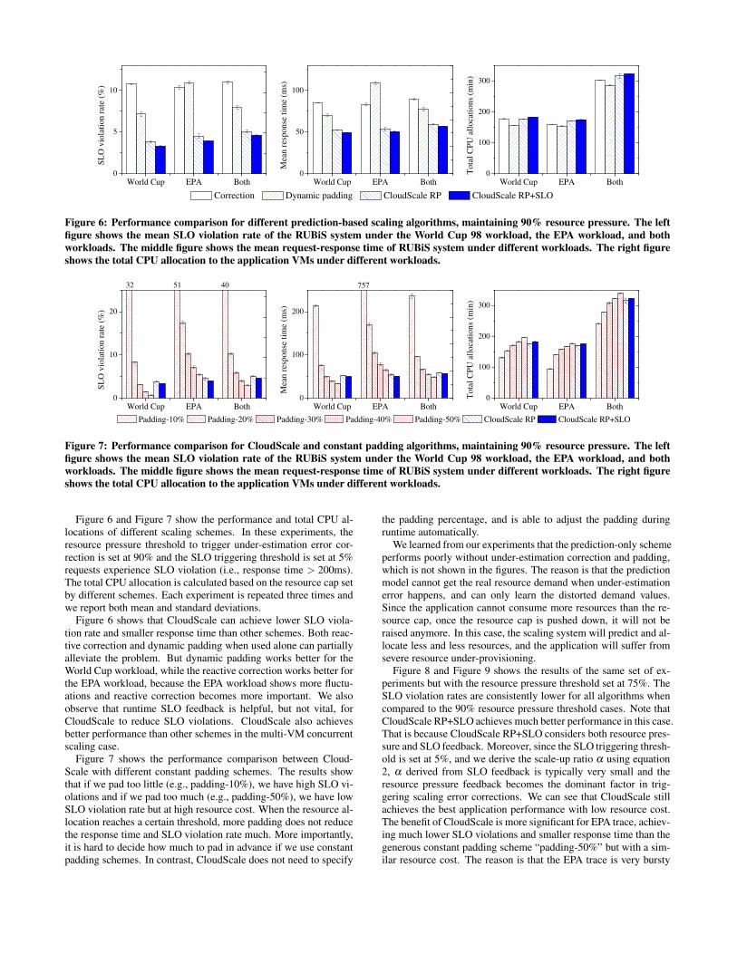
Figure 6: Performance comparison for different prediction-based scaling algorithms, maintaining 90% resource pressure. The left

figure shows the mean SLO violation rate of the RUBiS system under the World Cup 98 workload, the EPA workload, and both

workloads. The middle figure shows the mean request-response time of RUBiS system under different workloads. The right figure

shows the total CPU allocation to the application VMs under different workloads.

World Cup EPA Both0

10

20

405132

SL

O v

iola

tio

n r

ate

(%)

World Cup EPA Both0

100

200

757M

ean

res

po

nse

tim

e (m

s)

World Cup EPA Both0

100

200

300

To

tal

CP

U a

llo

cati

on

s (m

in)

Padding-10% Padding-20% Padding-30% Padding-40% Padding-50% CloudScale RP CloudScale RP+SLO

Figure 7: Performance comparison for CloudScale and constant padding algorithms, maintaining 90% resource pressure. The left




Figure 6 and Figure 7 show the performance and total CPU al-locations of different scaling schemes. In these experiments, theresource pressure threshold to trigger under-estimation error cor-rection is set at 90% and the SLO triggering threshold is set at 5%requests experience SLO violation (i.e., response time > 200ms).The total CPU allocation is calculated based on the resource cap setby different schemes. Each experiment is repeated three times andwe report both mean and standard deviations.

Figure 6 shows that CloudScale can achieve lower SLO viola-tion rate and smaller response time than other schemes. Both reac-tive correction and dynamic padding when used alone can partiallyalleviate the problem. But dynamic padding works better for theWorld Cup workload, while the reactive correction works better forthe EPA workload, because the EPA workload shows more fluctu-ations and reactive correction becomes more important. We alsoobserve that runtime SLO feedback is helpful, but not vital, forCloudScale to reduce SLO violations. CloudScale also achievesbetter performance than other schemes in the multi-VM concurrentscaling case.

Figure 7 shows the performance comparison between Cloud-Scale with different constant padding schemes. The results showthat if we pad too little (e.g., padding-10%), we have high SLO vi-olations and if we pad too much (e.g., padding-50%), we have lowSLO violation rate but at high resource cost. When the resource al-location reaches a certain threshold, more padding does not reducethe response time and SLO violation rate much. More importantly,it is hard to decide how much to pad in advance if we use constantpadding schemes. In contrast, CloudScale does not need to specify

the padding percentage, and is able to adjust the padding duringruntime automatically.

We learned from our experiments that the prediction-only schemeperforms poorly without under-estimation correction and padding,which is not shown in the figures. The reason is that the predictionmodel cannot get the real resource demand when under-estimationerror happens, and can only learn the distorted demand values.Since the application cannot consume more resources than the re-source cap, once the resource cap is pushed down, it will not beraised anymore. In this case, the scaling system will predict and al-locate less and less resources, and the application will suffer fromsevere resource under-provisioning.

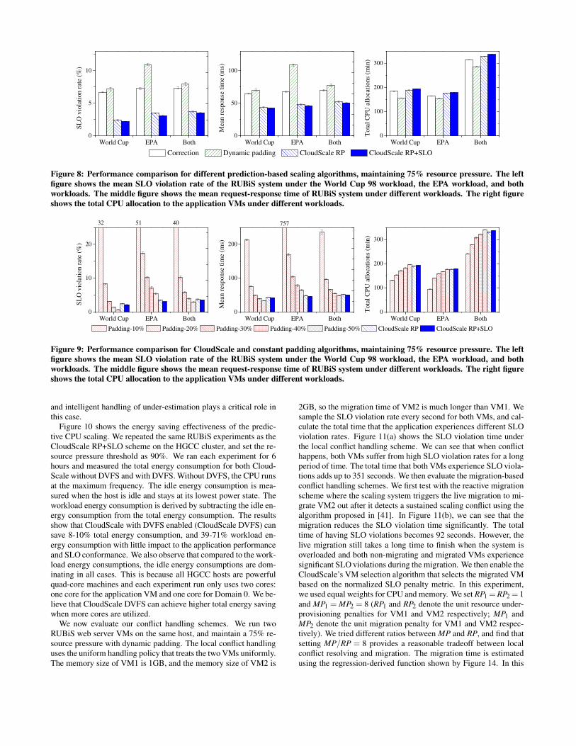
Figure 8 and Figure 9 shows the results of the same set of ex-periments but with the resource pressure threshold set at 75%. TheSLO violation rates are consistently lower for all algorithms whencompared to the 90% resource pressure threshold cases. Note thatCloudScale RP+SLO achieves much better performance in this case.That is because CloudScale RP+SLO considers both resource pres-sure and SLO feedback. Moreover, since the SLO triggering thresh-old is set at 5%, and we derive the scale-up ratio α using equation2, α derived from SLO feedback is typically very small and theresource pressure feedback becomes the dominant factor in trig-gering scaling error corrections. We can see that CloudScale stillachieves the best application performance with low resource cost.The benefit of CloudScale is more significant for EPA trace, achiev-ing much lower SLO violations and smaller response time than thegenerous constant padding scheme “padding-50%” but with a sim-ilar resource cost. The reason is that the EPA trace is very bursty

World Cup EPA Both0

5

10

SL

O v

iola

tio

n r

ate

(%)

World Cup EPA Both0

50

100

Mea

n r

esp

on

se t

ime

(ms)

World Cup EPA Both0

100

200

300

To

tal

CP

U a

llo

cati

on

s (m

in)

Correction Dynamic padding CloudScale RP CloudScale RP+SLO

Figure 8: Performance comparison for different prediction-based scaling algorithms, maintaining 75% resource pressure. The left




World Cup EPA Both0

10

20

SL

O v

iola

tio

n r

ate

(%)

World Cup EPA Both0

100

200

Mea

n r

esp

on

se t

ime

(ms)

World Cup EPA Both0

100

200

300

Padding-10% Padding-20% Padding-30% Padding-40% Padding-50% CloudScale RP CloudScale RP+SLO

To

tal

CP

U a

llo

cati

on

s (m

in)

405132 757

Figure 9: Performance comparison for CloudScale and constant padding algorithms, maintaining 75% resource pressure. The left




and intelligent handling of under-estimation plays a critical role inthis case.

Figure 10 shows the energy saving effectiveness of the predic-tive CPU scaling. We repeated the same RUBiS experiments as theCloudScale RP+SLO scheme on the HGCC cluster, and set the re-source pressure threshold as 90%. We ran each experiment for 6hours and measured the total energy consumption for both Cloud-Scale without DVFS and with DVFS. Without DVFS, the CPU runsat the maximum frequency. The idle energy consumption is mea-sured when the host is idle and stays at its lowest power state. Theworkload energy consumption is derived by subtracting the idle en-ergy consumption from the total energy consumption. The resultsshow that CloudScale with DVFS enabled (CloudScale DVFS) cansave 8-10% total energy consumption, and 39-71% workload en-ergy consumption with little impact to the application performanceand SLO conformance. We also observe that compared to the work-load energy consumptions, the idle energy consumptions are dom-inating in all cases. This is because all HGCC hosts are powerfulquad-core machines and each experiment run only uses two cores:one core for the application VM and one core for Domain 0. We be-lieve that CloudScale DVFS can achieve higher total energy savingwhen more cores are utilized.

We now evaluate our conflict handling schemes. We run twoRUBiS web server VMs on the same host, and maintain a 75% re-source pressure with dynamic padding. The local conflict handlinguses the uniform handling policy that treats the two VMs uniformly.The memory size of VM1 is 1GB, and the memory size of VM2 is

2GB, so the migration time of VM2 is much longer than VM1. Wesample the SLO violation rate every second for both VMs, and cal-culate the total time that the application experiences different SLOviolation rates. Figure 11(a) shows the SLO violation time underthe local conflict handling scheme. We can see that when conflicthappens, both VMs suffer from high SLO violation rates for a longperiod of time. The total time that both VMs experience SLO viola-tions adds up to 351 seconds. We then evaluate the migration-basedconflict handling schemes. We first test with the reactive migrationscheme where the scaling system triggers the live migration to mi-grate VM2 out after it detects a sustained scaling conflict using thealgorithm proposed in [41]. In Figure 11(b), we can see that themigration reduces the SLO violation time significantly. The totaltime of having SLO violations becomes 92 seconds. However, thelive migration still takes a long time to finish when the system isoverloaded and both non-migrating and migrated VMs experiencesignificant SLO violations during the migration. We then enable theCloudScale’s VM selection algorithm that selects the migrated VMbased on the normalized SLO penalty metric. In this experiment,we used equal weights for CPU and memory. We set RP1 =RP2 = 1and MP1 = MP2 = 8 (RP1 and RP2 denote the unit resource under-provisioning penalties for VM1 and VM2 respectively; MP1 andMP2 denote the unit migration penalty for VM1 and VM2 respec-tively). We tried different ratios between MP and RP, and find thatsetting MP/RP = 8 provides a reasonable tradeoff between localconflict resolving and migration. The migration time is estimatedusing the regression-derived function shown by Figure 14. In this

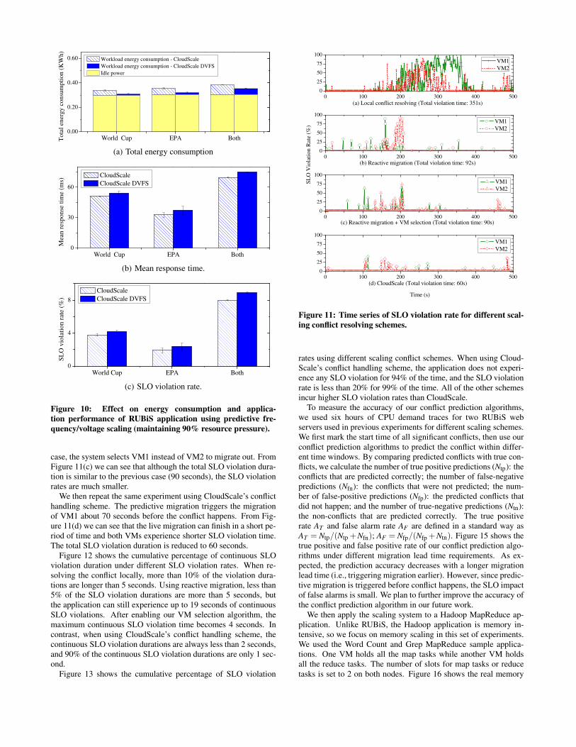
World Cup EPA Both0.00

0.20

0.40

0.60T

ota

l en

erg

y c

on

sum

pti

on

(K

Wh

) Workload energy consumption - CloudScale

Workload energy consumption - CloudScale DVFS

Idle power

(a) Total energy consumption

World Cup EPA Both0

30

60

Mea

n r

esp

on

se t

ime

(ms)

CloudScale

CloudScale DVFS

(b) Mean response time.

World Cup EPA Both0

4

8

SL

O v

iola

tio

n r

ate

(%)

CloudScale

CloudScale DVFS

(c) SLO violation rate.

Figure 10: Effect on energy consumption and applica-

tion performance of RUBiS application using predictive fre-

quency/voltage scaling (maintaining 90% resource pressure).

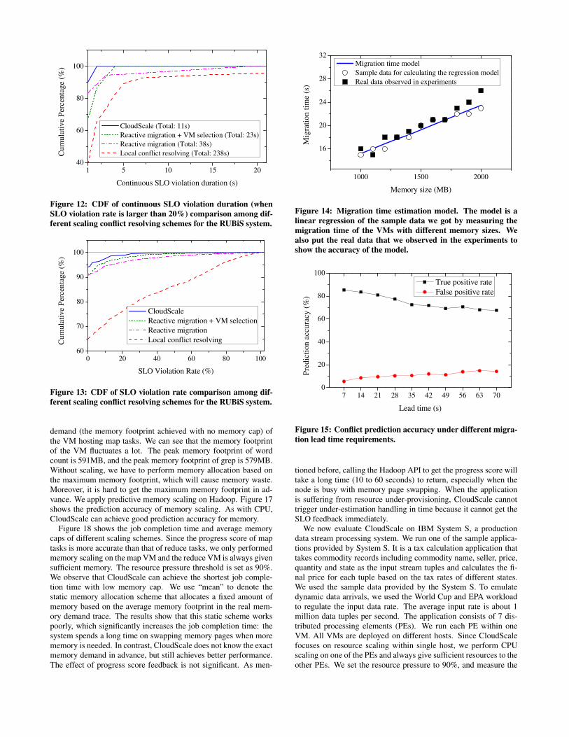
case, the system selects VM1 instead of VM2 to migrate out. FromFigure 11(c) we can see that although the total SLO violation dura-tion is similar to the previous case (90 seconds), the SLO violationrates are much smaller.

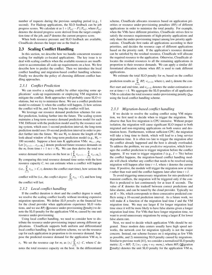
We then repeat the same experiment using CloudScale’s conflicthandling scheme. The predictive migration triggers the migrationof VM1 about 70 seconds before the conflict happens. From Fig-ure 11(d) we can see that the live migration can finish in a short pe-riod of time and both VMs experience shorter SLO violation time.The total SLO violation duration is reduced to 60 seconds.

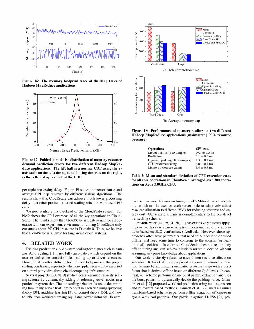
Figure 12 shows the cumulative percentage of continuous SLOviolation duration under different SLO violation rates. When re-solving the conflict locally, more than 10% of the violation dura-tions are longer than 5 seconds. Using reactive migration, less than5% of the SLO violation durations are more than 5 seconds, butthe application can still experience up to 19 seconds of continuousSLO violations. After enabling our VM selection algorithm, themaximum continuous SLO violation time becomes 4 seconds. Incontrast, when using CloudScale’s conflict handling scheme, thecontinuous SLO violation durations are always less than 2 seconds,and 90% of the continuous SLO violation durations are only 1 sec-ond.

Figure 13 shows the cumulative percentage of SLO violation

0 100 200 300 400 5000

25

50

75

100

(d) CloudScale (Total violation time: 60s)

(c) Reactive migration + VM selection (Total violation time: 90s)

(b) Reactive migration (Total violation time: 92s)

VM1

VM2

(a) Local conflict resolving (Total violation time: 351s)

0 100 200 300 400 5000

25

50

75

100

SL

O V

iola

tio

n R

ate

(%)

VM1

VM2

0 100 200 300 400 5000

25

50

75

100

Time (s)

VM1

VM2

0 100 200 300 400 5000

25

50

75

100

VM1

VM2

Figure 11: Time series of SLO violation rate for different scal-

ing conflict resolving schemes.

rates using different scaling conflict schemes. When using Cloud-Scale’s conflict handling scheme, the application does not experi-ence any SLO violation for 94% of the time, and the SLO violationrate is less than 20% for 99% of the time. All of the other schemesincur higher SLO violation rates than CloudScale.

To measure the accuracy of our conflict prediction algorithms,we used six hours of CPU demand traces for two RUBiS webservers used in previous experiments for different scaling schemes.We first mark the start time of all significant conflicts, then use ourconflict prediction algorithms to predict the conflict within differ-ent time windows. By comparing predicted conflicts with true con-flicts, we calculate the number of true positive predictions (Ntp): theconflicts that are predicted correctly; the number of false-negativepredictions (Nfn): the conflicts that were not predicted; the num-ber of false-positive predictions (Nfp): the predicted conflicts thatdid not happen; and the number of true-negative predictions (Ntn):the non-conflicts that are predicted correctly. The true positiverate AT and false alarm rate AF are defined in a standard way asAT = Ntp/(Ntp +Nfn); AF = Nfp/(Nfp +Ntn). Figure 15 shows thetrue positive and false positive rate of our conflict prediction algo-rithms under different migration lead time requirements. As ex-pected, the prediction accuracy decreases with a longer migrationlead time (i.e., triggering migration earlier). However, since predic-tive migration is triggered before conflict happens, the SLO impactof false alarms is small. We plan to further improve the accuracy ofthe conflict prediction algorithm in our future work.

We then apply the scaling system to a Hadoop MapReduce ap-plication. Unlike RUBiS, the Hadoop application is memory in-tensive, so we focus on memory scaling in this set of experiments.We used the Word Count and Grep MapReduce sample applica-tions. One VM holds all the map tasks while another VM holdsall the reduce tasks. The number of slots for map tasks or reducetasks is set to 2 on both nodes. Figure 16 shows the real memory

1 5 10 15 2040

60

80

100C

um

ula

tiv

e P

erce

nta

ge

(%)

Continuous SLO violation duration (s)

CloudScale (Total: 11s)

Reactive migration + VM selection (Total: 23s)

Reactive migration (Total: 38s)

Local conflict resolving (Total: 238s)

Figure 12: CDF of continuous SLO violation duration (when

SLO violation rate is larger than 20%) comparison among dif-

ferent scaling conflict resolving schemes for the RUBiS system.

0 20 40 60 80 10060

70

80

90

100

Cu

mu

lati

ve

Per

cen

tag

e (%

)

SLO Violation Rate (%)

CloudScale

Reactive migration + VM selection

Reactive migration

Local conflict resolving

Figure 13: CDF of SLO violation rate comparison among dif-

ferent scaling conflict resolving schemes for the RUBiS system.

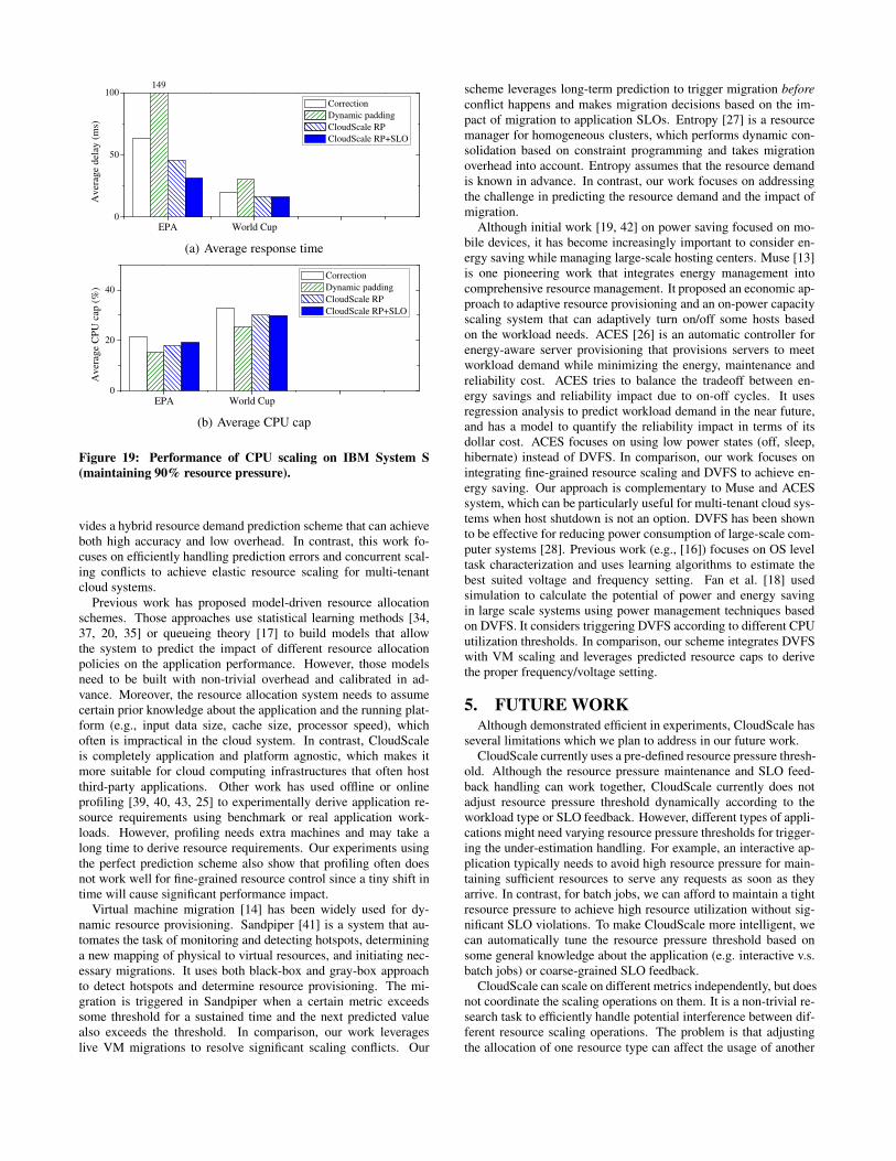
demand (the memory footprint achieved with no memory cap) ofthe VM hosting map tasks. We can see that the memory footprintof the VM fluctuates a lot. The peak memory footprint of wordcount is 591MB, and the peak memory footprint of grep is 579MB.Without scaling, we have to perform memory allocation based onthe maximum memory footprint, which will cause memory waste.Moreover, it is hard to get the maximum memory footprint in ad-vance. We apply predictive memory scaling on Hadoop. Figure 17shows the prediction accuracy of memory scaling. As with CPU,CloudScale can achieve good prediction accuracy for memory.

Figure 18 shows the job completion time and average memorycaps of different scaling schemes. Since the progress score of maptasks is more accurate than that of reduce tasks, we only performedmemory scaling on the map VM and the reduce VM is always givensufficient memory. The resource pressure threshold is set as 90%.We observe that CloudScale can achieve the shortest job comple-tion time with low memory cap. We use “mean” to denote thestatic memory allocation scheme that allocates a fixed amount ofmemory based on the average memory footprint in the real mem-ory demand trace. The results show that this static scheme workspoorly, which significantly increases the job completion time: thesystem spends a long time on swapping memory pages when morememory is needed. In contrast, CloudScale does not know the exactmemory demand in advance, but still achieves better performance.The effect of progress score feedback is not significant. As men-

1000 1500 2000

16

20

24

28

32

Mig

rati

on

tim

e (s

)

Memory size (MB)

Migration time model

Sample data for calculating the regression model

Real data observed in experiments

Figure 14: Migration time estimation model. The model is a

linear regression of the sample data we got by measuring the

migration time of the VMs with different memory sizes. We

also put the real data that we observed in the experiments to

show the accuracy of the model.

7 14 21 28 35 42 49 56 63 700

20

40

60

80

100

Pre

dic

tio

n a

ccu

racy

(%

)

Lead time (s)

True positive rate

False positive rate

Figure 15: Conflict prediction accuracy under different migra-

tion lead time requirements.

tioned before, calling the Hadoop API to get the progress score willtake a long time (10 to 60 seconds) to return, especially when thenode is busy with memory page swapping. When the applicationis suffering from resource under-provisioning, CloudScale cannottrigger under-estimation handling in time because it cannot get theSLO feedback immediately.

We now evaluate CloudScale on IBM System S, a productiondata stream processing system. We run one of the sample applica-tions provided by System S. It is a tax calculation application thattakes commodity records including commodity name, seller, price,quantity and state as the input stream tuples and calculates the fi-nal price for each tuple based on the tax rates of different states.We used the sample data provided by the System S. To emulatedynamic data arrivals, we used the World Cup and EPA workloadto regulate the input data rate. The average input rate is about 1million data tuples per second. The application consists of 7 dis-tributed processing elements (PEs). We run each PE within oneVM. All VMs are deployed on different hosts. Since CloudScalefocuses on resource scaling within single host, we perform CPUscaling on one of the PEs and always give sufficient resources to theother PEs. We set the resource pressure to 90%, and measure the

0 500 1000 1500 2000 25000

200

400

600

800 Word Count

Mem

ory

fo

otp

rin

t (M

B)

0 80 160 240 320 400 480 5600

200

400

600

Time (s)

Grep

Figure 16: The memory footprint trace of the Map tasks of

Hadoop MapReduce applications.

-300 -200 -100 0 100 200 3000

10

20

30

40

50

Cu

mu

lati

ve

Per

cen

tag

e (%

)

Memory Usage Prediction Error (MB)

Word Count

Grep

100

90

80

70

60

50

Figure 17: Folded cumulative distribution of memory resource

demand prediction errors for two different Hadoop MapRe-

duce applications. The left half is a normal CDF using the y-

axis scale on the left; the right half, using the scale on the right,

is the reflected upper half of the CDF.

per-tuple processing delay. Figure 19 shows the performance andaverage CPU cap achieved by different scaling algorithms. Theresults show that CloudScale can achieve much lower processingdelay than other prediction-based scaling schemes with low CPUcaps.

We now evaluate the overhead of the CloudScale system. Ta-ble 2 shows the CPU overhead of all the key operations in Cloud-Scale. The results show that CloudScale is light-weight for all op-erations. In our experiment environment, running CloudScale onlyconsumes about 2% CPU resource in Domain 0. Thus, we believethat CloudScale is suitable for large-scale cloud systems.

4. RELATED WORKExisting production cloud system scaling techniques such as Ama-

zon Auto Scaling [1] is not fully automatic, which depend on theuser to define the conditions for scaling up or down resources.However, it is often difficult for the user to figure out the properscaling conditions, especially when the application will be executedon a third-party virtualized cloud computing infrastructure.

Several projects [30, 38, 9] studied coarse-grained capacity scal-ing scheme by dynamically adding or releasing server nodes in aparticular system tier. The tier scaling schemes focus on determin-ing how many server hosts are needed in each tier using queueingtheory [38], machine learning [9], or control theory [30], and howto rebalance workload among replicated server instances. In com-

Word Count Grep0

2000

4000

6000

Job

co

mp

leti

on

tim

e (s

)

Mean

Correction

Dynamic padding

CloudScale RP

CloudScale RP+SLO

12828

(a) Job completion time

Word Count Grep0

200

400

600

Mea

n m

emo

ry f

oo

tpri

nt

(MB

)

Mean

Correction

Dynamic padding

CloudScale RP

CloudScale RP+SLO

(b) Average memory cap

Figure 18: Performance of memory scaling on two different

Hadoop MapReduce applications (maintaining 90% resource

pressure).

Operations CPU cost

Model training (100 samples) 69.7 ± 0.3 msPrediction 0.1 ± 0.0 msDynamic padding (100 samples) 1.3 ± 0.1 msCPU resource scaling 4.0 ± 0.1 msMemory resource scaling 9.4 ± 0.3 ms

Table 2: Mean and standard deviation of CPU execution costs

for all core operations in CloudScale, averaged over 300 opera-

tions on Xeon 3.0GHz CPU.

parison, our work focuses on fine-grained VM-level resource scal-ing, which can be used on each server node to adaptively adjustresource allocation to different VMs for reducing resource and en-ergy cost. Our scaling scheme is complementary to the host-leveltier scaling scheme.

Previous work [44, 29, 31, 36, 32] has extensively studied apply-ing control theory to achieve adaptive fine-grained resource alloca-tions based on SLO conformance feedback. However, those ap-proaches often have parameters that need to be specified or tunedoffline, and need some time to converge to the optimal (or near-optimal) decisions. In contrast, CloudScale does not require anyoffline tuning and can achieve elastic resource allocation withoutassuming any prior knowledge about applications.

Our work is closely related to trace-driven resource allocationschemes. Rolia et al. [33] proposed a dynamic resource alloca-tion scheme by multiplying estimated resource usage with a burstfactor that is derived offline based on different QoS levels. In con-trast, our scheme performs online burst pattern extraction and usesthe burst pattern to dynamically decide the padding value. Chan-dra et al. [12] proposed workload prediction using auto-regressionand histogram based methods. Gmach et al. [22] used a Fouriertransform-based scheme to perform offline extraction of long-termcyclic workload patterns. Our previous system PRESS [24] pro-

EPA World Cup0

50

100

Av

erag

e d

elay

(m

s) Correction

Dynamic padding

CloudScale RP

CloudScale RP+SLO

149

(a) Average response time

EPA World Cup0

20

40

Av

erag

e C

PU

cap

(%

)

Correction

Dynamic padding

CloudScale RP

CloudScale RP+SLO

(b) Average CPU cap

Figure 19: Performance of CPU scaling on IBM System S

(maintaining 90% resource pressure).

vides a hybrid resource demand prediction scheme that can achieveboth high accuracy and low overhead. In contrast, this work fo-cuses on efficiently handling prediction errors and concurrent scal-ing conflicts to achieve elastic resource scaling for multi-tenantcloud systems.

Previous work has proposed model-driven resource allocationschemes. Those approaches use statistical learning methods [34,37, 20, 35] or queueing theory [17] to build models that allowthe system to predict the impact of different resource allocationpolicies on the application performance. However, those modelsneed to be built with non-trivial overhead and calibrated in ad-vance. Moreover, the resource allocation system needs to assumecertain prior knowledge about the application and the running plat-form (e.g., input data size, cache size, processor speed), whichoften is impractical in the cloud system. In contrast, CloudScaleis completely application and platform agnostic, which makes itmore suitable for cloud computing infrastructures that often hostthird-party applications. Other work has used offline or onlineprofiling [39, 40, 43, 25] to experimentally derive application re-source requirements using benchmark or real application work-loads. However, profiling needs extra machines and may take along time to derive resource requirements. Our experiments usingthe perfect prediction scheme also show that profiling often doesnot work well for fine-grained resource control since a tiny shift intime will cause significant performance impact.

Virtual machine migration [14] has been widely used for dy-namic resource provisioning. Sandpiper [41] is a system that au-tomates the task of monitoring and detecting hotspots, determininga new mapping of physical to virtual resources, and initiating nec-essary migrations. It uses both black-box and gray-box approachto detect hotspots and determine resource provisioning. The mi-gration is triggered in Sandpiper when a certain metric exceedssome threshold for a sustained time and the next predicted valuealso exceeds the threshold. In comparison, our work leverageslive VM migrations to resolve significant scaling conflicts. Our

scheme leverages long-term prediction to trigger migration before

conflict happens and makes migration decisions based on the im-pact of migration to application SLOs. Entropy [27] is a resourcemanager for homogeneous clusters, which performs dynamic con-solidation based on constraint programming and takes migrationoverhead into account. Entropy assumes that the resource demandis known in advance. In contrast, our work focuses on addressingthe challenge in predicting the resource demand and the impact ofmigration.

Although initial work [19, 42] on power saving focused on mo-bile devices, it has become increasingly important to consider en-ergy saving while managing large-scale hosting centers. Muse [13]is one pioneering work that integrates energy management intocomprehensive resource management. It proposed an economic ap-proach to adaptive resource provisioning and an on-power capacityscaling system that can adaptively turn on/off some hosts basedon the workload needs. ACES [26] is an automatic controller forenergy-aware server provisioning that provisions servers to meetworkload demand while minimizing the energy, maintenance andreliability cost. ACES tries to balance the tradeoff between en-ergy savings and reliability impact due to on-off cycles. It usesregression analysis to predict workload demand in the near future,and has a model to quantify the reliability impact in terms of itsdollar cost. ACES focuses on using low power states (off, sleep,hibernate) instead of DVFS. In comparison, our work focuses onintegrating fine-grained resource scaling and DVFS to achieve en-ergy saving. Our approach is complementary to Muse and ACESsystem, which can be particularly useful for multi-tenant cloud sys-tems when host shutdown is not an option. DVFS has been shownto be effective for reducing power consumption of large-scale com-puter systems [28]. Previous work (e.g., [16]) focuses on OS leveltask characterization and uses learning algorithms to estimate thebest suited voltage and frequency setting. Fan et al. [18] usedsimulation to calculate the potential of power and energy savingin large scale systems using power management techniques basedon DVFS. It considers triggering DVFS according to different CPUutilization thresholds. In comparison, our scheme integrates DVFSwith VM scaling and leverages predicted resource caps to derivethe proper frequency/voltage setting.

5. FUTURE WORKAlthough demonstrated efficient in experiments, CloudScale has

several limitations which we plan to address in our future work.CloudScale currently uses a pre-defined resource pressure thresh-

old. Although the resource pressure maintenance and SLO feed-back handling can work together, CloudScale currently does notadjust resource pressure threshold dynamically according to theworkload type or SLO feedback. However, different types of appli-cations might need varying resource pressure thresholds for trigger-ing the under-estimation handling. For example, an interactive ap-plication typically needs to avoid high resource pressure for main-taining sufficient resources to serve any requests as soon as theyarrive. In contrast, for batch jobs, we can afford to maintain a tightresource pressure to achieve high resource utilization without sig-nificant SLO violations. To make CloudScale more intelligent, wecan automatically tune the resource pressure threshold based onsome general knowledge about the application (e.g. interactive v.s.batch jobs) or coarse-grained SLO feedback.

CloudScale can scale on different metrics independently, but doesnot coordinate the scaling operations on them. It is a non-trivial re-search task to efficiently handle potential interference between dif-ferent resource scaling operations. The problem is that adjustingthe allocation of one resource type can affect the usage of another

type of resource, which might introduce more dynamics into thesystem and cause more prediction errors. To address the problem,we plan to investigate multi-metric prediction model that can pre-dict multiple metrics together and scale them concurrently.

Similar to multi-metric scaling, it is also challenging to handlemulti-tier application scaling, in which different tiers have inter-dependency and scaling on one tier can affect the others. We canintegrate CloudScale with host-level scaling techniques [30, 38, 9]to handle multi-tier application scaling efficiently by predicting theresource demand of different tiers at the same time and coordinat-ing the scaling operation on different hosts.

CloudScale performs long-term conflict prediction by extractingthe repeating pattern in the resource usage trace. When the repeat-ing pattern is not found, CloudScale relies on multi-step Markovprediction algorithms for long-term predictions. However, multi-step Markov prediction has limited prediction accuracy since thecorrelation between the resource prediction model and the actualresource demand becomes weaker as we look further into the fu-ture. We are investigating other long-term prediction models to bet-ter handle the case when no periodic pattern is found in the trainingdata.

CloudScale currently works in the capping mode, which isolatesco-located applications by ensuring that the application cannot con-sume more resources than those allocated to it. Xen credit sched-uler also supports a weight mode: assigning each VM a weightwhich indicates the relative CPU share of the VM. CloudScale canbe easily extended to support weight mode by adjusting the weightof the VMs dynamically based on the resource demand prediction.In contrast to the capping mode, VMs can consume residual CPUresources out of their shares in weight mode. However, when re-source contention happens, weight mode cannot provide perfor-mance isolation, and it is impossible to know the real demand ofthe collocated VMs since their resource usages are affected by eachother. As a future work, we will leverage our conflict predictionto dynamically switch between capping mode and weight mode.When there is no conflict, CloudScale can work in weight mode toimprove the resource utilization. When there are conflicts, Cloud-Scale can work in capping mode to ensure performance isolation.

6. CONCLUSIONIn this paper, we presented CloudScale, an automatic elastic re-

source scaling system for multi-tenant cloud computing infrastruc-tures. CloudScale consists of three key components: 1) combin-ing online resource demand prediction and efficient prediction er-ror handling to meet application SLOs with minimum resourcecost; 2) supporting multi-VM concurrent scaling with conflict pre-diction and predicted migration to resolve scaling conflicts withminimum SLO impact; and 3) integrating VM resource scalingwith dynamic voltage and frequency scaling (DVFS) to save en-ergy without affecting application SLOs. We have implementedCloudScale on top of the Xen virtualization platform and conductedextensive experiments using the RUBiS benchmark driven by realWeb server traces, Hadoop MapReduce systems, and a commer-cial stream processing system. The experimental results show thatCloudScale can achieve much better SLO conformance than otheralternative schemes with low resource cost. CloudScale can re-solve scaling conflicts with up to 83% less SLO violation time thanother schemes. CloudScale can save 8-10% total energy consump-tion, and 39-71% workload energy consumption with little impactto the application performance and SLO conformance. CloudScaleis light-weight and application-agnostic, which makes it suitablefor large-scale cloud systems.

7. ACKNOWLEDGEMENTThis work was sponsored in part by NSF CNS0915567 grant,

NSF CNS0915861 grant, U.S. Army Research Office (ARO) un-der grant W911NF-10-1-0273, and Google Research Awards. Anyopinions expressed in this paper are those of the authors and donot necessarily reflect the views of the NSF, ARO, or U.S. Govern-ment. The authors thank the anonymous reviewers for their insight-ful comments.

8. REFERENCES

[1] Amazon Elastic Compute Cloud.http://aws.amazon.com/ec2/.

[2] Apache Hadoop System. http://hadoop.apache.org/core/.

[3] KVM (Kernel-based Virtual Machine).http://www.linux-kvm.org/page/Main_Page.

[4] RUBiS Online Auction System. http://rubis.ow2.org/.

[5] The IRCache Project. http://www.ircache.net/.

[6] Virtual Computing Lab. http://vcl.ncsu.edu/.

[7] VMware Virtualization Technology.http://www.vmware.com/.

[8] Xen Credit Scheduler.http://wiki.xensource.com/xenwiki/CreditScheduler.

[9] M. Armbrust, A. Fox, D. A. Patterson, N. Lanham,B. Trushkowsky, J. Trutna, and H. Oh. Scads:Scale-independent storage for social computing applications.In Proc. CIDR, 2009.

[10] P. Barham and et al. Xen and the art of virtualization. InProc. SOSP, 2003.

[11] D. Breitgand, M. B.-Yehuda, M. Factor, H. Kolodner,V. Kravtsov, and D. Pelleg. NAP: a building block forremediating performance bottlenecks via black box networkanalysis. In Proc. ICAC, 2009.

[12] A. Chandra, W. Gong, and P. Shenoy. Dynamic resourceallocation for shared data centers using onlinemeasurements. In Proc. IWQoS, 2004.

[13] J. Chase, D. Anderson, P. N. Thakar, and A. M. Vahdat.Managing energy and server resources in hosting centers. InProc. SOSP, 2001.

[14] C. Clark, K. Fraser, S. Hand, J. G. Hansen, E. Jul,C. Limpach, I. Pratt, and A. Warfield. Live migration ofvirtual machines. In Proc. NSDI, 2005.

[15] J. Dean and S. Ghemawat. MapReduce: Simplified dataprocessing on large clusters. Dec. 2004.

[16] G. Dhiman and T. S. Rosing. Dynamic voltage frequencyscaling for multi-tasking systems using online learning. InProc. ISLPED, 2007.

[17] R. Doyle, J. Chase, O. Asad, W. Jin, and A. Vahdat.Model-based resource provisioning in a web service utility.In Proc. USITS, 2003.

[18] X. Fan, W.-D. Weber, and L. A. Barroso. Power provisioningfor a warehouse-sized computer. In Proc. ISCA, 2007.

[19] J. Flinn and M. Satyanarayanan. Energy-aware adaptation formobile applications. In Proc. SOSP, 1999.

[20] A. Ganapathi, H. Kuno, and et al. Predicting multiple metricsfor queries: Better decisions enabled by machine learning. InProc. ICDE, 2009.

[21] B. Gedik, H. Andrade, K.-L. Wu, P. S. Yu, and M. Doo.SPADE: the System S declarative stream processing engine.Proc. SIGMOD, 2008.

[22] D. Gmach, J. Rolia, L. Cherkasova, and A. Kemper. Capacity

management and demand prediction for next generation datacenters. In Proc. ICWS, 2007.

[23] Z. Gong and X. Gu. PAC: Pattern-driven ApplicationConsolidation for Efficient Cloud Computing. In Proc.

MASCOTS, 2010.

[24] Z. Gong, X. Gu, and J. Wilkes. PRESS: PRedictive ElasticReSource Scaling for Cloud Systems. In Proc. CNSM, 2010.

[25] S. Govindan, J. Choi, and et al. Statistical profiling-basedtechniques for effective power provisioning in data centers.In Proc. Eurosys, 2009.

[26] B. Guenter, N. Jain, and C. Williams. Managing cost,performance, and reliability tradeoffs for energy-awareserver provisioning. In Proc. INFOCOM, 2011.

[27] F. Hermenier, X. Lorca, J.-M. Menaud, G. Muller, andJ. Lawall. Entropy: a consolidation manager for clusters. InProc. VEE, 2009.

[28] C.-H. Hsu and W.-C. Feng. A power-aware run-time systemfor high-performance computing. In Proc. SC, 2005.

[29] E. Kalyvianaki, T. Charalambous, and S. Hand. Self-adaptiveand self-configured CPU resource provisioning forvirtualized servers using Kalman filters. In Proc. ICAC,2009.

[30] H. Lim, S. Babu, and J. Chase. Automated control for elasticstorage. In Proc. ICAC, 2010.

[31] P. Padala and et al. Adaptive control of virtualized resourcesin utility computing environments. In Proc. Eurosys, 2007.

[32] P. Padala, K.-Y. Hou, K. G. Shin, X. Zhu, M. Uysal,Z. Wang, S. Singhal, and A. Merchant. Automated control ofmultiple virtualized resources. In Proc. Eurosys, 2009.

[33] J. Rolia, L. Cherkasova, M. Arlitt, and V. Machiraju.Supporting application QoS in shared resource pools.Communications of the ACM, 2006.

[34] P. Shivam, S. Babu, and J. Chase. Learning applicationmodels for utility resource planning. In Proc. USITS, 2003.

[35] P. Shivam, S. Babu, and J. Chase. Active and acceleratedlearning of cost models for optimizing scientific applications.In Proc. VLDB, 2006.

[36] S.S.Parekh, N.Gandhi, J.L.Hellerstein, D.M.Tilbury,T. Jayram, and J. P. Bigus. Using control theory to achieveservice level objectives in performance management. In Real

Time Systems, 2002.

[37] C. Stewart, T. Kelly, A. Zhang, and K. Shen. A dollar from15 cents: cross-platform management for internet services.In Proc. USENIX Annual Technical Conference, 2008.

[38] B. Urgaonkar, M. S. G. Pacifici, P. J. Shenoy, and A. N.Tantawi. An analytical model for multi-tier internet servicesand its applications. In Proc. SIGMETRICS, 2005.

[39] B. Urgaonkar, P. Shenoy, and et al. Resource overbookingand application profiling in shared hosting platforms. InProc. OSDI, 2002.

[40] T. Wood, L. Cherkasova, and et al. Profiling and modelingresource usage of virtualized applications. In Proc.

Middleware, 2008.

[41] T. Wood, P. J. Shenoy, A. Venkataramani, and M. S. Yousif.Black-box and gray-box strategies for virtual machinemigration. In Proc. NSDI, 2007.

[42] W. Yuan and K. Nahrstedt. Energy-efficient soft real-timeCPU scheduling for mobile multimedia systems. In Proc.

SOSP, 2003.

[43] W. Zheng, R. Bianchini, and et al. JustRunIt:

Experiment-based management of virtualized data centers.In Proc. USENIX Annual Technical Conference, 2009.

[44] X. Zhu and et al. 1000 Islands: integrated capacity andworkload management for the next generation data center. InProc. ICAC, June 2008.

[45] X. Zhu, Z. Wang, and S. Singhal. Utility-driven workloadmanagement using nested control design. In Proc. American

Control Conference, 2006.

Documents

CloudScale: Elastic Resource Scaling for Multi-Tenant