Embed Size (px)
Citation preview

[19:42 26/2/2009 5283-Millsap-Ch20.tex] Job No: 5283 Millsap: The SAGE Handbook of Quantitative Methods in Psychology Page: 444 444–513
20Cluster Analysis: A Toolbox
for MATLABLawrence Hubert , Hans-Fr iedr ich Köhn,
and Douglas Steinley
INTRODUCTION
A broad definition of clustering can be given as the search for homogeneous groupings of objectsbased on some type of available data. There are two common such tasks now discussed in (almost)all multivariate analysis texts and implemented in the commercially available behavioral andsocial science statistical software suites: hierarchical clustering and the K-means partitioning ofsome set of objects. This chapter begins with a brief review of these topics using two illustrativedata sets that are carried along throughout this chapter for numerical illustration. Later sectionswill develop hierarchical clustering through least-squares and the characterizing notion of anultrametric; K-means partitioning is generalized by rephrasing as an optimization problem ofsubdividing a given proximity matrix. In all instances, the MATLAB computational environmentis relied on to effect our analyses, using the Statistical Toolbox, for example, to carry out the com-mon hierarchical clustering and K-means methods, and our own open-source MATLAB M-fileswhen the extensions go beyond what is currently available commercially (the latter are freelyavailable as a Toolbox from www.cda.psych.uiuc.edu/clusteranalysis_mfiles). Also, to maintaina reasonable printed size for the present handbook contribution, the table of contents, figures,and tables for the full chapter, plus the final section and the header comments for the M-files inAppendix A, are available from www.cda.psych.uiuc.edu/cluster_analysis_parttwo.pdf
A proximity matrix for illustrating hierarchical clustering: agreementamong Supreme Court justices
On Saturday, 2 July 2005, the lead headline in The NewYork Times read as follows: “O’Connor toRetire, Touching Off Battle Over Court.” Opening the story attached to the headline, Richard W.Stevenson wrote, “Justice Sandra Day O’Connor, the first woman to serve on the United StatesSupreme Court and a critical swing vote on abortion and a host of other divisive social issues,

[19:42 26/2/2009 5283-Millsap-Ch20.tex] Job No: 5283 Millsap: The SAGE Handbook of Quantitative Methods in Psychology Page: 445 444–513
CLUSTER ANALYSIS 445
Table 20.1 Dissimilarities among nine Supreme Court justices
St Br Gi So Oc Ke Re Sc Th
1 St .00 .38 .34 .37 .67 .64 .75 .86 .852 Br .38 .00 .28 .29 .45 .53 .57 .75 .763 Gi .34 .28 .00 .22 .53 .51 .57 .72 .744 So .37 .29 .22 .00 .45 .50 .56 .69 .715 Oc .67 .45 .53 .45 .00 .33 .29 .46 .466 Ke .64 .53 .51 .50 .33 .00 .23 .42 .417 Re .75 .57 .57 .56 .29 .23 .00 .34 .328 Sc .86 .75 .72 .69 .46 .42 .34 .00 .219 Th .85 .76 .74 .71 .46 .41 .32 .21 .00
announced Friday that she is retiring, setting up a tumultuous fight over her successor.” Ourinterests are in the data set also provided by the Times that day, quantifying the (dis)agreementamong the Supreme Court justices during the decade they had been together. We give this inTable 20.1 in the form of the percentage of non-unanimous cases in which the justices disagree,from the 1994/95 term through 2003/04 (known as the Rehnquist Court). The dissimilaritymatrix (in which larger entries reflect less similar justices) is listed in the same row and columnorder as the Times data set, with the justices ordered from “liberal” to “conservative”:
1: John Paul Stevens (St)2: Stephen G. Breyer (Br)3: Ruth Bader Ginsberg (Gi)4: David Souter (So)5: Sandra Day O’Connor (Oc)6: Anthony M. Kennedy (Ke)7: William H. Rehnquist (Re)8: Antonin Scalia (Sc)9: Clarence Thomas (Th)
We use the Supreme Court data matrix of Table 20.1 for the various illustrations of hierarchicalclustering in the sections to follow. It will be loaded into a MATLAB environment with thecommand ‘load supreme_agree.dat’. The supreme_agree.dat file is in simpleascii form with verbatim contents as follows:
.00 .38 .34 .37 .67 .64 .75 .86 .85
.38 .00 .28 .29 .45 .53 .57 .75 .76
.34 .28 .00 .22 .53 .51 .57 .72 .74
.37 .29 .22 .00 .45 .50 .56 .69 .71
.67 .45 .53 .45 .00 .33 .29 .46 .46
.64 .53 .51 .50 .33 .00 .23 .42 .41
.75 .57 .57 .56 .29 .23 .00 .34 .32
.86 .75 .72 .69 .46 .42 .34 .00 .21
.85 .76 .74 .71 .46 .41 .32 .21 .00
A data set for illustrating K -means partitioning: the famous 1976blind tasting of French and California wines
In the bicentennial year for the United States of 1976, an Englishman, Steven Spurrier, andhis American partner, Patricia Gallagher, hosted a blind wine tasting in Paris that comparedCalifornia cabernet from Napa Valley and French cabernet from Bordeaux. Besides Spurrier and

[19:42 26/2/2009 5283-Millsap-Ch20.tex] Job No: 5283 Millsap: The SAGE Handbook of Quantitative Methods in Psychology Page: 446 444–513
446 DATA ANALYSIS
Table 20.2 Taster ratings among ten cabernets
Taster
Wine 1 2 3 4 5 6 7 8 9 10 11
A (US) 14 15 10 14 15 16 14 14 13 16.5 14B (F) 16 14 15 15 12 16 12 14 11 16 14C (F) 12 16 11 14 12 17 14 14 14 11 15D (F) 17 15 12 12 12 13.5 10 8 14 17 15E (US) 13 9 12 16 7 7 12 14 17 15.5 11F (F) 10 10 10 14 12 11 12 12 12 8 12G (US) 12 7 11.5 17 2 8 10 13 15 10 9H (US) 14 5 11 13 2 9 10 11 13 16.5 7I (US) 5 12 8 9 13 9.5 14 9 12 3 13J (US) 7 7 15 15 5 9 8 13 14 6 7
Gallagher, the nine other judges were notable French wine connoisseurs (the raters are listedbelow). The six California and four French wines are also identified below with the ratingsgiven in Table 20.2 (from 0 to 20 with higher scores being “better”). The overall conclusion isthat Stag’s Leap, a US offering, is the winner. (For those familiar with late 1950s TV, one canhear Sergeant Preston exclaiming “sacré bleu”, and wrapping up with, “Well King, this case isclosed”.) Our concern later will be in clustering the wines through the K-means procedure.
Tasters:
1: Pierre Brejoux, Institute of Appellations of Origin2: Aubert de Villaine, Manager, Domaine de la Romanée-Conti3: Michel Dovaz, Wine Institute of France4: Patricia Gallagher, L’Académie du Vin5: Odette Kahn, Director, Review of French Wines6: Christian Millau, Le Nouveau Guide (restaurant guide)7: Raymond Oliver, Owner, Le Grand Vefour8: Steven Spurrier, L’Académie du Vin9: Pierre Tart, Owner, Chateau Giscours
10: Christian Vanneque, Sommelier, La Tour D’Argent11: Jean-Claude Vrinat, Taillevent
Cabernet sauvignons:
A: Stag’s Leap 1973 (US)B: Château Mouton Rothschild 1970 (F)C: Château Montrose 1970 (F)D: Château Haut Brion 1970 (F)E: Ridge Monte Bello 1971 (US)F: Château Léoville-Las-Cases 1971 (F)G: Heitz “Martha’s Vineyard” 1970 (US)H: Clos du Val 1972 (US)I: Mayacamas 1971 (US)J: Freemark Abbey 1969 (US)
HIERARCHICAL CLUSTERING
To characterize the basic problem posed by hierarchical clustering somewhat more formally,suppose S is a set of n objects, {O1, . . . , On} [for example, in line with the two data

[19:42 26/2/2009 5283-Millsap-Ch20.tex] Job No: 5283 Millsap: The SAGE Handbook of Quantitative Methods in Psychology Page: 447 444–513
CLUSTER ANALYSIS 447
sets just given, the objects could be supreme court justices, wines, or tasters (e.g., ratersor judges)]. Between each pair of objects, Oi and Oj, a symmetric proximity measure,pij, is given or possibly constructed that we assume (from now on) has a dissimilarityinterpretation; these values are collected into an n × n proximity matrix P = {pij}n×n,such as the 9 × 9 example given in Table 20.1 among the supreme court justices.Any hierarchical clustering strategy produces a sequence or hierarchy of partitions of S,denoted P0, P1, . . . ,Pn−1, from the information present in P. In particular, the (disjoint)partition P0 contains all objects in separate classes, Pn−1 (the conjoint partition) consistsof one all-inclusive object class, and Pk+1 is defined from Pk by uniting a single pair ofsubsets in Pk .
Generally, the two subsets chosen to unite in defining Pk+1 from Pk are those that are“closest”, with the characterization of this latter term specifying the particular hierarchicalclustering method used. We mention three of the most common options for this notion ofcloseness:
1. Complete link: The maximum proximity value attained for pairs of objects within the union of two sets [thus,we minimize the maximum link or the subset ‘diameter’].
2. Single link: The minimum proximity value attained for pairs of objects, where the two objects from the pairbelong to the separate classes (thus, we minimize the minimum link).
3. Average link: The average proximity over pairs of objects defined across the separate classes (thus, weminimize the average link).
We generally suggest that the complete-link criterion be the default selection for thetask of hierarchical clustering when done in the traditional agglomerative way that startsfrom P0 and proceeds step-by-step to Pn−1. A reliance on single link tends to produce“straggly” clusters that are not very internally homogeneous nor substantively interpretable;the average-link choice seems to produce results that are the same as or very similarto the complete-link criterion but relies on more information from the given proximities;complete-link depends only on the rank order of the proximities. [As we anticipate fromlater discussion, the average-link criterion has some connections with rephrasing hierarchicalclustering as a least-squares optimization task in which an ultrametric (to be defined) isfit to the given proximity matrix. The average proximities between subsets characterize thefitted values.]
A complete-link clustering of the supreme_agree data set is given by the MATLABrecording below, along with the displayed dendrogram in Figure 20.1. [The later dendrogram isdrawn directly from the MATLAB Statistical Toolbox routines except for our added two-letterlabels for the justices (referred to as ‘terminal’ nodes in the dendrogram), and the numberingof the ‘internal’ nodes from 10 to 17 that represent the new subsets formed in the hierarchy.]The squareform M-function from the Statistics Toolbox changes a square proximity matrixwith zeros along the main diagonal to one in vector form that can be used in the main clusteringroutine, linkage. The results of the complete-link clustering are given by the 8 × 3 matrix(supreme_ agree_clustering), indicating how the objects (labeled from 1 to 9) andclusters (labeled 10 through 17) are formed and at what level. Here, the levels are the maximumproximities (or diameters) for the newly constructed subsets as the hierarchy is generated.These newly formed clusters (generally, n − 1 in number) are labeled in Figure 20.1 alongwith the calibration on the vertical axis as to when they are formed (we note that the terminalnode order in Figure 20.1 does not conform to the Justice order of Table 20.1; there is nooption to impose such an order on the dendrogram function in MATLAB. When a dendrogramis done “by hand”, however, it may be possible to impose such an order (see, for example,Figure 20.2).

[19:42 26/2/2009 5283-Millsap-Ch20.tex] Job No: 5283 Millsap: The SAGE Handbook of Quantitative Methods in Psychology Page: 448 444–513
448 DATA ANALYSIS
8 9 5 6 7 1 2 3 4
0.2
0.3
0.4
0.5
0.6
0.7
0.8
Sc Th Oc Ke Re St Br Gi So
10
16
14
12
15
13
11
17
Figure 20.1 Dendrogram representation for the complete-link hierarchical clustering of theSupreme Court proximity matrix.
The results could also be given as a sequence of partitions:
Partition Level formed
{{Sc,Th,Oc,Ke,Re,St,Br,Gi,So}} .86{{Sc,Th,Oc,Ke,Re},{St,Br,Gi,So}} .46
{{Sc,Th},{Oc,Ke,Re},{St,Br,Gi,So}} .38{{Sc,Th},{Oc,Ke,Re},{St},{Br,Gi,So}} .33
{{Sc,Th},{Oc},{Ke,Re},{St},{Br,Gi,So}} .29{{Sc,Th},{Oc},{Ke,Re},{St},{Br},{Gi,So}} .23
{{Sc,Th},{Oc},{Ke},{Re},{St},{Be},{Gi,So}} .22{{Sc,Th},{Oc},{Ke},{Re},{St},{Br},{Gi},{So}} .21
{{Sc},{Th},{Oc},{Ke},{Re},{St},{Br},{Gi},{So}} —
>> load supreme_agree.dat
>> supreme_agree
supreme_agree =
0 0.3800 0.3400 0.3700 0.6700 0.6400 0.7500 0.8600 0.8500
0.3800 0 0.2800 0.2900 0.4500 0.5300 0.5700 0.7500 0.7600
0.3400 0.2800 0 0.2200 0.5300 0.5100 0.5700 0.7200 0.7400
0.3700 0.2900 0.2200 0 0.4500 0.5000 0.5600 0.6900 0.7100
0.6700 0.4500 0.5300 0.4500 0 0.3300 0.2900 0.4600 0.4600
0.6400 0.5300 0.5100 0.5000 0.3300 0 0.2300 0.4200 0.4100
0.7500 0.5700 0.5700 0.5600 0.2900 0.2300 0 0.3400 0.3200
0.8600 0.7500 0.7200 0.6900 0.4600 0.4200 0.3400 0 0.2100
0.8500 0.7600 0.7400 0.7100 0.4600 0.4100 0.3200 0.2100 0
>> supreme_agree_vector = squareform(supreme_agree)
[19:42 26/2/2009 5283-Millsap-Ch20.tex] Job No: 5283 Millsap: The SAGE Handbook of Quantitative Methods in Psychology Page: 449 444–513
CLUSTER ANALYSIS 449
St Br Gi So Oc Ke Re Sc Th
.21 .22.23
.29
.31
.36
.40
.64
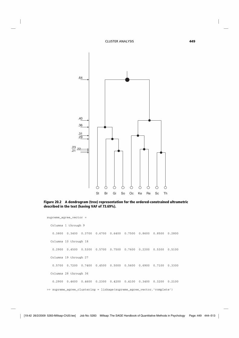
Figure 20.2 A dendrogram (tree) representation for the ordered-constrained ultrametricdescribed in the text (having VAF of 73.69%).
supreme_agree_vector =
Columns 1 through 9
0.3800 0.3400 0.3700 0.6700 0.6400 0.7500 0.8600 0.8500 0.2800
Columns 10 through 18
0.2900 0.4500 0.5300 0.5700 0.7500 0.7600 0.2200 0.5300 0.5100
Columns 19 through 27
0.5700 0.7200 0.7400 0.4500 0.5000 0.5600 0.6900 0.7100 0.3300
Columns 28 through 36
0.2900 0.4600 0.4600 0.2300 0.4200 0.4100 0.3400 0.3200 0.2100
>> supreme_agree_clustering = linkage(supreme_agree_vector,’complete’)

[19:42 26/2/2009 5283-Millsap-Ch20.tex] Job No: 5283 Millsap: The SAGE Handbook of Quantitative Methods in Psychology Page: 450 444–513
450 DATA ANALYSIS
supreme_agree_clustering =
8.0000 9.0000 0.21003.0000 4.0000 0.22006.0000 7.0000 0.23002.0000 11.0000 0.29005.0000 12.0000 0.33001.0000 13.0000 0.380010.0000 14.0000 0.460015.0000 16.0000 0.8600
>> dendrogram(supreme_agree_clustering)
Substantively, the interpretation of the complete-link hierarchical clustering result is veryclear. There are three “tight” dyads in {Sc,Th}, {Gi,So}, and {Ke,Re}; {Oc} joins with {Ke,Re},and {Br} with {Gi,So} to form, respectively, the “moderate” conservative and liberal clusters.{St} then joins with {Br,Gi,So} to form the liberal-left four-object cluster; {Oc,Ke,Re} uniteswith the dyad of {Sc,Th} to form the five-object conservative-right. All of this is not verysurprising given the enormous literature on the Rehnquist Court. What is satisfying from adata analyst’s perspective is how very clear the interpretation is, based on the dendrogram ofFigure 20.1 constructed empirically from the data of Table 20.1.
Ultrametrics
Given the partition hierarchies from any of the three criteria mentioned (complete, single, oraverage link), suppose we place the values for when the new subsets were formed (i.e., themaximum, minimum, or average proximity between the united subsets) into an n × n matrix Uwith rows and columns relabeled to conform with the order of display for the terminal nodesin the dendrogram. For example, Table 20.3 provides the complete-link results for U with anoverlay partitioning of the matrix to indicate the hierarchical clustering. In general, there aren − 1 distinct nonzero values that define the levels at which the n − 1 new subsets are formedin the hierarchy; thus, there are typically n − 1 distinct nonzero values present in a matrixU characterizing the identical blocks of matrix entries between subsets united in forming thehierarchy.
Given a matrix such as U, the partition hierarchy can be retrieved immediately along withthe levels at which the new subsets were formed. For example, Table 20.3, incorporating subsetdiameters (i.e., the maximum proximity within a subset) to characterize when formation takesplace, can be used to obtain the dendrogram and the explicit listing of the partitions in thehierarchy. In fact, any (strictly) monotone (i.e., order preserving) transformation of the n − 1
Table 20.3 Ultrametric values (based on subset diameters) characterizing the complete-linkhierarchical clustering of Table 20.1
Sc Th Oc Ke Re St Br Gi So
8 Sc .00 .21 .46 .46 .46 .86 .86 .86 .869 Th .21 .00 .46 .46 .46 .86 .86 .86 .865 Oc .46 .46 .00 .33 .33 .86 .86 .86 .866 Ke .46 .46 .33 .00 .23 .86 .86 .86 .867 Re .46 .46 .33 .23 .00 .86 .86 .86 .861 St .86 .86 .86 .86 .86 .00 .38 .38 .382 Br .86 .86 .86 .86 .86 .38 .00 .29 .293 Gi .86 .86 .86 .86 .86 .38 .29 .00 .224 So .86 .86 .86 .86 .86 .38 .29 .22 .00

[19:42 26/2/2009 5283-Millsap-Ch20.tex] Job No: 5283 Millsap: The SAGE Handbook of Quantitative Methods in Psychology Page: 451 444–513
CLUSTER ANALYSIS 451
distinct values in such a matrix U would serve the same retrieval purposes. Thus, as an example,we could replace the eight distinct values in Table 20.3, (.21, .22, .23, .29, .33, .38, .46, .86), bythe simple integers (1, 2, 3, 4, 5, 6, 7, 8), and the topology (i.e., the branching pattern) of thedendrogram and the partitions of the hierarchy could be reconstructed. Generally, we characterizea matrix U that can be used to retrieve a partition hierarchy in this way as an ultrametric:
A matrix U = {uij}n×n is ultrametric if for every triple of subscripts, i, j, and k, uij ≤max(uik, ukj); or equivalently (and much more understandably), among the three terms, uij,uik , and ukj, the largest two values are equal.
As can be verified, Table 20.3 (or any strictly monotone transformation of its entries) isultrametric; it can be used to retrieve a partition hierarchy, and the (n − 1 distinct nonzero)values in U define the levels at which the n − 1 new subsets are formed. The hierarchicalclustering task will be characterized in a later section as an optimization problem in which weseek to identify a best-fitting ultrametric matrix, say U∗, for a given proximity matrix P.
K -MEANS PARTITIONING
The data on which a K-means clustering is defined will be assumed in the form of a usual n × pdata matrix, X = {xij}, for n subjects over p variables. We will use the example of Table 20.2,where there are n = 10 wines (subjects) and p = 11 tasters (variables). Although we willnot pursue the notion here, there is typically a duality present in all such data matrices, andattention could be refocused on grouping tasters based on the wines now reconsidered to bethe “variables”.) If the set S = {O1, . . . , On} defines the n objects to be clustered, we seek acollection of K mutually exclusive and exhaustive subsets of S, say, C1, . . . , CK , that minimizesthe sum-of-squared-error (SSE):
SSE =K∑
k=1
∑
Oi∈Ck
p∑
j=1
(xij − mkj)2 (1)
for mkj = 1nk
∑Oi∈Ck
xij (the mean in group Ck on variable j), and nk , the number of objects in Ck .What this represents in the context of the usual univariate analysis-of-variance is a minimizationof the within-group sum-of-squares aggregated over the p variables in the data matrix X. Wealso note that for the most inward expression in (1), the term
∑pj=1(xij − mkj)2 represents the
squared Euclidean distance between the profile values over the p variables present for object Oi
and the variable means (or centroid) within the cluster Ck containing Oi (it is these latter Kcentroids or mean vectors that lend the common name of K-means).
The typical relocation algorithm would proceed as follows: an initial set of “seeds”(e.g., objects) is chosen and the sum-of-squared-error criterion is defined based on the distancesto these seeds. A reallocation of objects to groups is carried out according to minimum distance,and centroids recalculated. The minimum distance allocation and recalculation of centroidsis performed until no change is possible—each object is closest to the group centroid towhich it is now assigned. Note that at the completion of this stage, the solution will belocally optimal with respect to each object being closest to its group centroid. A final checkcan be made to determine if any single-object reallocations will reduce the sum-of-squared-error any further; at the completion of this stage, the solution will be locally optimal withrespect to (1).
We present a verbatim MATLAB session below in which we ask for two to four clusters forthe wines using the kmeans routine from the Statistical Toolbox on the cabernet_taste

[19:42 26/2/2009 5283-Millsap-Ch20.tex] Job No: 5283 Millsap: The SAGE Handbook of Quantitative Methods in Psychology Page: 452 444–513
452 DATA ANALYSIS
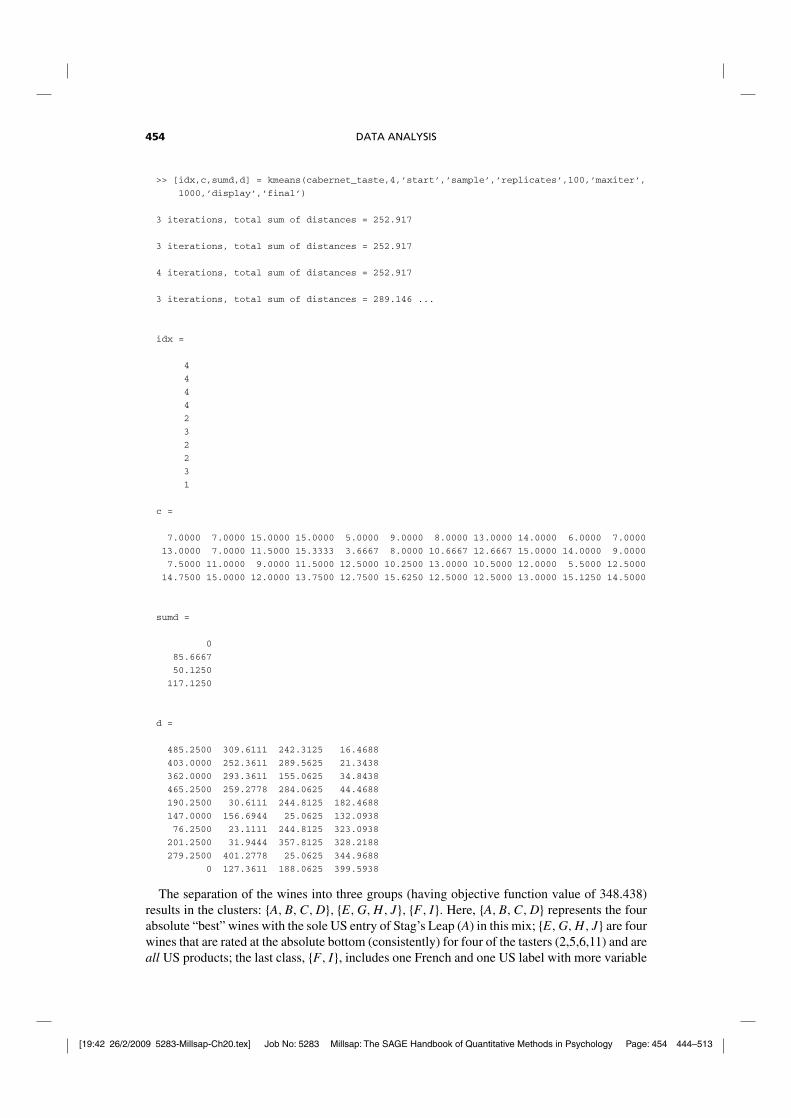
data matrix from Table 20.2. We choose one-hundred random starts (‘replicates’,100)by picking two to four objects at random to serve as the initial seeds (‘start’,‘sample’).Two local optima were found for the choice of two clusters, but only one for three.The control phrase (‘maxiter’,1000) increases the allowable number of iterations;(‘display’,‘final’) controls printing the end results for each of the hundred replications;most of this latter output is suppressed to save space and replaced by … ). The results actuallydisplayed for each number of chosen clusters are the best obtained over the hundred replicationswithidx indicating cluster membership for the n objects;c contains the cluster centroids;sumdgives the within-cluster sum of object-to-centroid distances (so when the entries are summed, theobjective function in (1) is generated); d includes all the distances between each object and eachcentroid.
>> load cabernet_taste.dat
>> cabernet_taste
cabernet_taste =
14.0000 15.0000 10.0000 14.0000 15.0000 16.0000 14.0000 14.0000 13.0000 16.5000 14.0000
16.0000 14.0000 15.0000 15.0000 12.0000 16.0000 12.0000 14.0000 11.0000 16.0000 14.0000
12.0000 16.0000 11.0000 14.0000 12.0000 17.0000 14.0000 14.0000 14.0000 11.0000 15.0000
17.0000 15.0000 12.0000 12.0000 12.0000 13.5000 10.0000 8.0000 14.0000 17.0000 15.0000
13.0000 9.0000 12.0000 16.0000 7.0000 7.0000 12.0000 14.0000 17.0000 15.5000 11.0000
10.0000 10.0000 10.0000 14.0000 12.0000 11.0000 12.0000 12.0000 12.0000 8.0000 12.0000
12.0000 7.0000 11.5000 17.0000 2.0000 8.0000 10.0000 13.0000 15.0000 10.0000 9.0000
14.0000 5.0000 11.0000 13.0000 2.0000 9.0000 10.0000 11.0000 13.0000 16.5000 7.0000
5.0000 12.0000 8.0000 9.0000 13.0000 9.5000 14.0000 9.0000 12.0000 3.0000 13.0000
7.0000 7.0000 15.0000 15.0000 5.0000 9.0000 8.0000 13.0000 14.0000 6.0000 7.0000
>> [idx,c,sumd,d] = kmeans(cabernet_taste,2,’start’,’sample’,’replicates’,100,’maxiter’,
1000,’display’,’final’)
2 iterations, total sum of distances = 633.208
3 iterations, total sum of distances = 633.063 ...
idx =
2
2
2
2
1
2
1
1
2
1
c =
11.5000 7.0000 12.3750 15.2500 4.0000 8.2500 10.0000 12.7500 14.7500 12.0000 8.5000
12.3333 13.6667 11.0000 13.0000 12.6667 13.8333 12.6667 11.8333 12.6667 11.9167 13.8333
sumd =
181.1875
451.8750

[19:42 26/2/2009 5283-Millsap-Ch20.tex] Job No: 5283 Millsap: The SAGE Handbook of Quantitative Methods in Psychology Page: 453 444–513
CLUSTER ANALYSIS 453
d =
329.6406 44.3125
266.1406 63.3125
286.6406 27.4792
286.8906 76.8958
46.6406 155.8125
130.3906 48.9792
12.5156 249.5625
50.3906 290.6458
346.8906 190.8958
71.6406 281.6458
----------------------------------------------------------------------------------------
>> [idx,c,sumd,d] = kmeans(cabernet_taste,3,’start’,’sample’,’replicates’,100,’maxiter’,
1000,’display’,’final’)
3 iterations, total sum of distances = 348.438 ...
idx =
1
1
1
1
2
3
2
2
3
2
c =
14.7500 15.0000 12.0000 13.7500 12.7500 15.6250 12.5000 12.5000 13.0000 15.1250 14.5000
11.5000 7.0000 12.3750 15.2500 4.0000 8.2500 10.0000 12.7500 14.7500 12.0000 8.5000
7.5000 11.0000 9.0000 11.5000 12.5000 10.2500 13.0000 10.5000 12.0000 5.5000 12.5000
sumd =
117.1250
181.1875
50.1250
d =
16.4688 329.6406 242.3125
21.3438 266.1406 289.5625
34.8438 286.6406 155.0625
44.4688 286.8906 284.0625
182.4688 46.6406 244.8125
132.0938 130.3906 25.0625
323.0938 12.5156 244.8125
328.2188 50.3906 357.8125
344.9688 346.8906 25.0625
399.5938 71.6406 188.0625
---------------------------------------------------------------------------------------
[19:42 26/2/2009 5283-Millsap-Ch20.tex] Job No: 5283 Millsap: The SAGE Handbook of Quantitative Methods in Psychology Page: 454 444–513
454 DATA ANALYSIS
>> [idx,c,sumd,d] = kmeans(cabernet_taste,4,’start’,’sample’,’replicates’,100,’maxiter’,
1000,’display’,’final’)
3 iterations, total sum of distances = 252.917
3 iterations, total sum of distances = 252.917
4 iterations, total sum of distances = 252.917
3 iterations, total sum of distances = 289.146 ...
idx =
4
4
4
4
2
3
2
2
3
1
c =
7.0000 7.0000 15.0000 15.0000 5.0000 9.0000 8.0000 13.0000 14.0000 6.0000 7.0000
13.0000 7.0000 11.5000 15.3333 3.6667 8.0000 10.6667 12.6667 15.0000 14.0000 9.0000
7.5000 11.0000 9.0000 11.5000 12.5000 10.2500 13.0000 10.5000 12.0000 5.5000 12.5000
14.7500 15.0000 12.0000 13.7500 12.7500 15.6250 12.5000 12.5000 13.0000 15.1250 14.5000
sumd =
0
85.6667
50.1250
117.1250
d =
485.2500 309.6111 242.3125 16.4688
403.0000 252.3611 289.5625 21.3438
362.0000 293.3611 155.0625 34.8438
465.2500 259.2778 284.0625 44.4688
190.2500 30.6111 244.8125 182.4688
147.0000 156.6944 25.0625 132.0938
76.2500 23.1111 244.8125 323.0938
201.2500 31.9444 357.8125 328.2188
279.2500 401.2778 25.0625 344.9688
0 127.3611 188.0625 399.5938
The separation of the wines into three groups (having objective function value of 348.438)results in the clusters: {A, B, C, D}, {E, G, H, J}, {F, I}. Here, {A, B, C, D} represents the fourabsolute “best” wines with the sole US entry of Stag’s Leap (A) in this mix; {E, G, H, J} are fourwines that are rated at the absolute bottom (consistently) for four of the tasters (2,5,6,11) and areall US products; the last class, {F, I}, includes one French and one US label with more variable

[19:42 26/2/2009 5283-Millsap-Ch20.tex] Job No: 5283 Millsap: The SAGE Handbook of Quantitative Methods in Psychology Page: 455 444–513
CLUSTER ANALYSIS 455
ratings over the judges. This latter group also coalesces with the best group when only twoclusters are sought. From a nonchauvinistic perspective, the presence of the single US offeringof Stag’s Leap in the “best” group of four (within the three-class solution) does not say verystrongly to us that the US has somehow “won”.
K -means and matrix partitioning
The most inward expression in (1):
∑
Oi∈Ck
p∑
j=1
(xij − mkj)2 (2)
can be interpreted as the sum of the squared Euclidean distances between every object in Ck andthe centroid for this cluster. These sums are aggregated, in turn, over k (from 1 to K) to obtainthe sum-of-squared-error criterion that we attempt to minimize in K-means clustering by thejudicious choice of C1, . . . , CK . Alternatively, the expression in (2) can be re-expressed as:
1
2nk
∑
Oi,Oi′ ∈Ck
p∑
j=1
(xij − xi′j)2 (3)
or a quantity equal to the sum of the squared Euclidean distances between all object pairs in Ck
divided by twice the number of objects, nk , in Ck . If we define the proximity, pii′ , between anytwo objects, Oi and Oi′ , over the p variables as the squared Euclidean distance, then (3) couldbe rewritten as:
1
2nk
∑
Oi,Oi′ ∈Ck
pii′ (4)
Or, consider the proximity matrix P = {pii′ } and for any clustering, C1, . . . , CK , the proximitymatrix can be schematically represented as:
C1 · · · Ck · · · CK
C1 P11 · · · P1k · · · P1K...
... · · · ... · · · ...
Ck Pk1 · · · Pkk · · · PkK...
... · · · ... · · · ...
CK PK1 · · · PKk · · · PKK
where the objects in S have been reordered so each cluster Ck represents a contiguoussegment of (ordered objects) and Pkk′ is the nk × nk′ collection of proximities betweenthe objects in Ck and Ck′ . In short, the sum-of-squared-error criterion is merely the sumof proximities in Pkk weighted by 1
2nkand aggregated over k from 1 to K (i.e., the sum
of the main diagonal blocks of P). In fact, any clustering evaluated with the sum-of-squared-error criterion could be represented by such a structure defined with a reorderedproximity matrix having its rows and columns grouped to contain the contiguous objectsin C1, . . . , CK .
To give an example of this kind of proximity matrix for our cabernet example, the squaredEuclidean distance matrix among the wines is given in Table 20.4 with the row and column

[19:42 26/2/2009 5283-Millsap-Ch20.tex] Job No: 5283 Millsap: The SAGE Handbook of Quantitative Methods in Psychology Page: 456 444–513
456 DATA ANALYSIS
Table 20.4 Squared Euclidean distances among ten cabernetsClassWine C1/A C1/B C1/C C1/D C2/E C2/G C2/H C2/J C3/F C3/I
C1/A .00 48.25 48.25 86.50 220.00 400.50 394.00 485.25 160.25 374.50C1/B 48.25 .00 77.00 77.25 195.25 327.25 320.25 403.00 176.00 453.25C1/C 48.25 77.00 .00 131.25 229.25 326.25 410.25 362.00 107.00 253.25C1/D 86.50 77.25 131.25 .00 202.50 355.50 305.50 465.25 202.25 416.00
C2/E 220.00 195.25 229.25 202.50 .00 75.50 102.00 190.25 145.25 394.50C2/G 400.50 327.25 326.25 355.50 75.50 .00 79.50 76.25 160.25 379.50C2/H 394.00 320.25 410.25 305.50 102.00 79.50 .00 201.25 250.25 515.50C2/J 485.25 403.00 362.00 465.25 190.25 76.25 201.25 .00 147.00 279.25
C3/F 160.25 176.00 107.00 202.25 145.25 160.25 250.25 147.00 .00 100.25C3/I 374.50 453.25 253.25 416.00 394.50 379.50 515.50 279.25 100.25 .00
objects reordered to conform to the three-group K-means clustering. The expression in (3) inrelation to Table 20.4 would be given as:
1
2n1
∑
Oi,Oi′ ∈C1
pii′ + 1
2n2
∑
Oi,Oi′ ∈C2
pii′ + 1
2n3
∑
Oi,Oi′ ∈C3
pii′
= 1
2(4)(937.00) + 1
2(4)(1449.50) + 1
2(2)(200.50)
= 117.1250 + 181.1875 + 50.1250 = 348.438 (5)
This is the same objective function value from (1) reported in the verbatim MATLAB output.
BEYOND THE BASICS: EXTENSIONS OF HIERARCHICAL CLUSTERING ANDK -MEANS PARTITIONING
Abrief introduction to the two dominant tasks of hierarchical clustering and K-means partitioninghave been provided in the previous two sections. Here, several extensions of these ideas willbe discussed to make the analysis techniques generally more useful to the user. In contrastto earlier sections, where the cited MATLAB routines were already part of the StatisticsToolbox, the M-files from this section on are available (open-source) from the authors’ web site:www.http://cda.psych.uiuc.edu/ clusteranalysis_mfilesWe provide thehelp “header” files for all of these M-files in an Appendix A to this chapter; these shouldbe generally helpful in explaining both syntax and usage. The four subsections below dealsuccessively with the following topics (with examples to follow thereafter).
(a) The hierarchical clustering task can be reformulated as locating a best-fitting ultrametric,say U∗ = {u∗
ij}, to the given proximity matrix, P, such that the least-squares criterion:
∑
i<j
(pij − u∗ij)
2 , (6)
is minimized. The approach can either be confirmatory (in which we look for the best-fittingultrametric defined by some monotone transformation of the n − 1 values making up a fixedultrametric), or exploratory (where we merely look for the best-fitting ultrametric without anyprior constraint as to its form). In both cases, a convenient normalized loss measure is given by

[19:42 26/2/2009 5283-Millsap-Ch20.tex] Job No: 5283 Millsap: The SAGE Handbook of Quantitative Methods in Psychology Page: 457 444–513
CLUSTER ANALYSIS 457
the variance-accounted-for (VAF):
VAF = 1 −∑
i<j(pij − u∗ij)
2
∑i<j(pij − p̄)2
, (7)
where p̄ is the average off-diagonal proximity value in P. This is directly comparable to theusual VAF measure familiar from multiple regression.
(b) In identifying a best-fitting ultrametric and displaying it subsequently through adendrogram, there is a degree of arbitrariness in how the terminal nodes are ordered. If wetreat the dendrogram as a “mobile” and allow the internal nodes to act as universal joints withfreedom of 360◦ degree rotation, there are 2n−1 equivalent orderings of the terminal nodes (inour example, 28 is 256), and none is preferred a priori. To impose some meaning on the terminalnode ordering, we provide two routines that either impose a given ordering or look for a “best”one that could be used for display in the exploratory identification of a best-fitting ultrametric.These routines rely on a preliminary identification of a least-squares best-fitting anti-Robinsonmatrix (an anti-Robinson (AR) matrix is one in which the entries never decrease when movingwithin the rows or columns away from the main diagonal entries). Treating the fittedAR matrix asthe collection of “proximities” in their own right, the process of finding a best-fitting ultrametricis then carried out, producing a dendrogram that is consistently displayable with respect to theconstraining order. In effect, we are combining the two (somewhat) different tasks of hierarchicalclustering and the seriation of an object set by reordering the rows and columns of P to displayas closely as possible, a particularly appealing AR gradient in its entries.
(c) In observing that the K-means criterion could be reinterpreted through a proximity matrixdefined by squared Euclidean distances, it was also noted that the clusters could be representedas contiguous segments of ordered objects in a reordered proximity matrix. We exploit thisconnection by rephrasing the search for the better (in the sense of hopefully being moresubstantively interpretable) partitions by imposing a preliminary order on the squared Euclideanproximity matrix; then, for a given number of clusters, a (globally) optimal subdivision is foundbased on the K-means criterion [the M-file that carries this out is an implementation of anorder-constrained dynamic programming (DP) routine that can handle a very large number ofobjects with guaranteed (order-constrained) optimality for the traditional K-means criterion].It appears that this tandem strategy of finding an order first and then carrying out a K-meanssubdivision, does well in its generation of substantively interpretable partitions. It is as if weare simultaneously optimizing two objective functions—one that provides a typically goodapproximate AR ordering for the squared Euclidean distances (an AR ordering that, in fact,might be interpretable more-or-less “as is”), and a second that is not prone to the local optimumproblem plaguing all K-means iterative methods because it is based on a DPstrategy guaranteeingglobal optimality (albeit within an order-constrained context).
(d) The idea of providing an optimal mechanism for subdividing an order-constrainedproximity matrix (and not one just based on squared Euclidean distances), gives a natural meansfor generalizing the usual (agglomerative) hierarchical clustering methods, such as complete-or average-link. Defining a good preliminary constraining order for the proximity matrix, anoptimization routine (based on DP) is implemented that will give optimal partitions into 2 ton − 1 classes respecting the preliminary order (having classes containing objects contiguouswith respect to it), and minimizing the maximum such measure obtained over the classesmaking up the partitions (the maximum proximity [or diameter] within a class for the complete-link criterion; the average of the proximities within a class for the average-link criterion). The“minimum of the maximum” is used because otherwise a tendency will exist to produce justone large class for each optimal partition; also, this seems a closer analogue to agglomerative

[19:42 26/2/2009 5283-Millsap-Ch20.tex] Job No: 5283 Millsap: The SAGE Handbook of Quantitative Methods in Psychology Page: 458 444–513
458 DATA ANALYSIS
hierarchical clustering when we try to minimize a maximum as each partition is constructedfrom the proceeding one. Stated alternatively, the best single partition optimization analogueto hierarchical clustering, with the latter’s myopic process and greedy “best it can do” at eachnext level, would be the optimization goal of minimizing the maximum subset measure overthe classes of a partition. In the case of our K-means interpretation in (c), a simple sum over theclasses can be optimized that does not generally lead to the “one big class” triviality, apparentlybecause of the divisions by twice the number of objects within each class in the specific lossfunction used in the optimization.
A useful utility: obtaining a constraining order
In implementing an order-constrained K-means clustering strategy, an appropriate initialordering must be generated to constrain the clustering in the first place.Although many strategiesmight be considered, a particularly powerful one appears definable through what is called thequadratic assignment (QA) task and a collection of local-improvement optimization heuristics.As typically defined, a QA problem involves two n × n matrices, A = {aij} and T = {tij}, andwe seek a permutation to maximize the cross-product statistic:
�(ρ) =∑
i �=j
aρ(i)ρ(j)tij (8)
The notation {aρ(i)ρ(j)} implies a reordering (by the permutation ρ(·)) of the rows andsimultaneously the columns of A so that the rows (and columns) now appear in the orderρ(1) � ρ(2) � · · · � ρ(n). For our purposes, the first matrix A could be identified withthe proximity matrix P containing squared Euclidean distances between the subject profilesover the p variables; the second matrix contains a target defined by a set of locations equally-spaced along a line, i.e., T = {|j − i|} for 1 ≤ i, j ≤ n. (More generally, P could be anyproximity matrix having a dissimilarity interpretation; use of the resulting identified permutation,for example, would be one way of implementing an order-constrained DP proximity matrixsubdivision.)
In attempting to find ρ to maximize �(ρ), we try to reorganize the proximity matrix asPρ = {pρ(i)ρ(j)}, to show the same pattern, more or less, as the fixed target T; equivalently,we maximize the usual Pearson product-moment correlation between the off-diagonal entriesin T and Pρ . Another way of rephrasing this search is to say that we seek a permutation ρ
that provides a structure as “close” as possible to an AR form for Pρ , i.e., the degree to whichthe entries in Pρ , moving away from the main diagonal in either direction never decrease (andusually increase); this is exactly the pattern exhibited by the equally spaced target matrix T. Inour order-constrained K-means application, once the proximity matrix is so reordered by ρ, welook for a K-means clustering result that respects the order generating the “as close as we canget to an AR” patterning for the row/column permuted matrix.
The type of heuristic optimization strategy we use for the QA task implements simpleobject interchange/rearrangement operations. Based on given matrices A and T, and beginningwith some permutation (possibly chosen at random), local interchanges and rearrangementsof a particular type are implemented until no improvement in the index can be made.By repeatedly initializing such a process randomly, a distribution over a set of local optimacan be achieved. Three different classes of local operations are used in the M-file, order.m:(i) the pairwise interchanges of objects in the current permutation defining the row and columnorder of the data matrix A. All possible such interchanges are generated and considered inturn, and whenever an increase in the cross-product index would result from a particular

[19:42 26/2/2009 5283-Millsap-Ch20.tex] Job No: 5283 Millsap: The SAGE Handbook of Quantitative Methods in Psychology Page: 459 444–513
CLUSTER ANALYSIS 459
interchange, it is made immediately. The process continues until the current permutation cannotbe improved upon by any such pairwise object interchange. The procedure then proceedsto (ii): the local operations considered are all reinsertions of from 1 to kblock (which isless than n and set by the user) consecutive objects somewhere in the permutation definingthe current row and column order of the data matrix. When no further improvement can bemade, we move to (iii): the local operations are now all possible rotations (or inversions)of from 2 to kblock consecutive objects in the current row/column order of the datamatrix. (We suggest a use of kblock equal to 3 as a reasonable compromise between theextensiveness of local search, speed of execution, and quality of solution.) The three collectionsof local changes are revisited (in order) until no alteration is possible in the final permutationobtained.
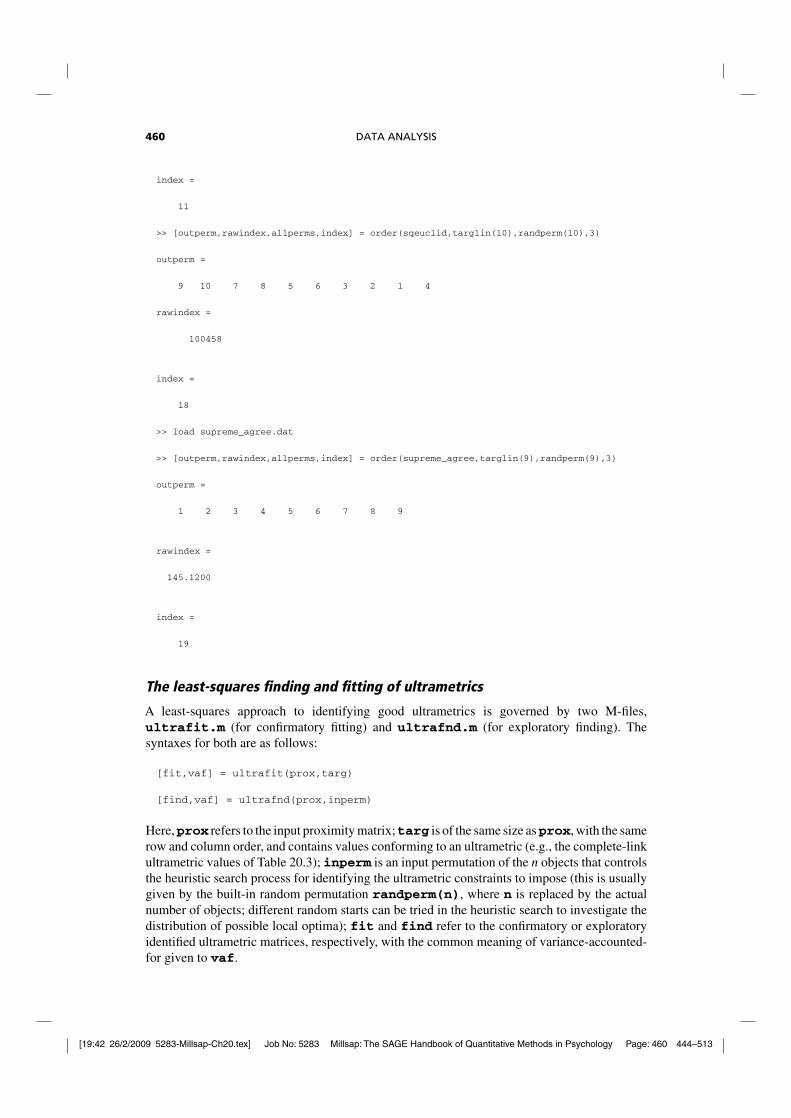
The use of order.m is illustrated in the verbatim recording below, first on the squaredEuclidean distance matrix among the ten cabernets (see Table 20.4) to produce the constrainingorder used in the order-constrained K-means clustering subsection below. Among the twolocal optima found, we will choose the one with the higher rawindex in (8) of 100,458,and corresponding to the order in outperm of [9 10 7 8 5 6 3 2 1 4]. There are indexpermutations stored in the MATLAB cell-array allperms, from the first randomly generatedone in allperms{1}, to the found local optimum in allperms{index}. (These havebeen suppressed in the output.) Notice that retrieving entries in a cell array requires the useof curly braces, {,}. The M-file, targlin.m, provides the equally-spaced target matrix asan input. We also show that starting with a random permutation and the supreme_agreedata matrix, the identity permutation is retrieved (in fact, it would be the sole local optimumfound upon repeated starts using random permutations). It might be noted that an empiricallyconstructed constraining order for an ultrametric (which leads in turn to a best-fitting AR matrix)is carried out with exactly this same type of QA routine (and used internally in the M-file,ultrafnd_confnd.m, discussed in a subsection to follow).
>> load cabernet_taste.dat
>> [sqeuclid] = sqeuclidean(cabernet_taste)
sqeuclid =
0 48.2500 48.2500 86.5000 220.0000 160.2500 400.5000 394.0000 374.5000 485.2500
48.2500 0 77.0000 77.2500 195.2500 176.0000 327.2500 320.2500 453.2500 403.0000
48.2500 77.0000 0 131.2500 229.2500 107.0000 326.2500 410.2500 253.2500 362.0000
86.5000 77.2500 131.2500 0 202.5000 202.2500 355.5000 305.5000 416.0000 465.2500
220.0000 195.2500 229.2500 202.5000 0 145.2500 75.5000 102.0000 394.5000 190.2500
160.2500 176.0000 107.0000 202.2500 145.2500 0 160.2500 250.2500 100.2500 147.0000
400.5000 327.2500 326.2500 355.5000 75.5000 160.2500 0 79.5000 379.5000 76.2500
394.0000 320.2500 410.2500 305.5000 102.0000 250.2500 79.5000 0 515.5000 201.2500
374.5000 453.2500 253.2500 416.0000 394.5000 100.2500 379.5000 515.5000 0 279.2500
485.2500 403.0000 362.0000 465.2500 190.2500 147.0000 76.2500 201.2500 279.2500 0
>> [outperm,rawindex,allperms,index] = order(sqeuclid,targlin(10),randperm(10),3)
outperm =
10 8 7 5 6 2 4 3 1 9
rawindex =
100333
[19:42 26/2/2009 5283-Millsap-Ch20.tex] Job No: 5283 Millsap: The SAGE Handbook of Quantitative Methods in Psychology Page: 460 444–513
460 DATA ANALYSIS
index =
11
>> [outperm,rawindex,allperms,index] = order(sqeuclid,targlin(10),randperm(10),3)
outperm =
9 10 7 8 5 6 3 2 1 4
rawindex =
100458
index =
18
>> load supreme_agree.dat
>> [outperm,rawindex,allperms,index] = order(supreme_agree,targlin(9),randperm(9),3)
outperm =
1 2 3 4 5 6 7 8 9
rawindex =
145.1200
index =
19
The least-squares finding and fitting of ultrametrics
A least-squares approach to identifying good ultrametrics is governed by two M-files,ultrafit.m (for confirmatory fitting) and ultrafnd.m (for exploratory finding). Thesyntaxes for both are as follows:
[fit,vaf] = ultrafit(prox,targ)
[find,vaf] = ultrafnd(prox,inperm)
Here,prox refers to the input proximity matrix;targ is of the same size asprox, with the samerow and column order, and contains values conforming to an ultrametric (e.g., the complete-linkultrametric values of Table 20.3); inperm is an input permutation of the n objects that controlsthe heuristic search process for identifying the ultrametric constraints to impose (this is usuallygiven by the built-in random permutation randperm(n), where n is replaced by the actualnumber of objects; different random starts can be tried in the heuristic search to investigate thedistribution of possible local optima); fit and find refer to the confirmatory or exploratoryidentified ultrametric matrices, respectively, with the common meaning of variance-accounted-for given to vaf.

[19:42 26/2/2009 5283-Millsap-Ch20.tex] Job No: 5283 Millsap: The SAGE Handbook of Quantitative Methods in Psychology Page: 461 444–513
CLUSTER ANALYSIS 461
A MATLAB session using these two functions is reproduced below. The complete-link targetultrametric matrix, sc_completelink_target, with the same row and column ordering assupreme_agree induces a least-squares confirmatory fitted matrix having VAF of 73.69%.The monotonic function, say f (·), between the values of the fitted and input target matrices canbe given as follows: f (.21) = .21; f (.22) = .22; f (.23) = .23; f (.29) = .2850; f (.33) =.31; f (.38) = .3633; f (.46) = .4017; f (.86) = .6405. Interestingly, an exploratory use ofultrafnd.m produces exactly this same result; also, there appears to be only this one localoptimum identifiable over many random starts (these results are not explicitly reported here butcan be replicated easily by the reader. Thus, at least for this particular data set, the complete-link method produces the optimal (least-squares) branching structure as verified over repeatedrandom initializations for ultrafnd.m).
>> load sc_completelink_target.dat
>> sc_completelink_target
sc_completelink_target =
0 0.3800 0.3800 0.3800 0.8600 0.8600 0.8600 0.8600 0.86000.3800 0 0.2900 0.2900 0.8600 0.8600 0.8600 0.8600 0.86000.3800 0.2900 0 0.2200 0.8600 0.8600 0.8600 0.8600 0.86000.3800 0.2900 0.2200 0 0.8600 0.8600 0.8600 0.8600 0.86000.8600 0.8600 0.8600 0.8600 0 0.3300 0.3300 0.4600 0.46000.8600 0.8600 0.8600 0.8600 0.3300 0 0.2300 0.4600 0.46000.8600 0.8600 0.8600 0.8600 0.3300 0.2300 0 0.4600 0.46000.8600 0.8600 0.8600 0.8600 0.4600 0.4600 0.4600 0 0.21000.8600 0.8600 0.8600 0.8600 0.4600 0.4600 0.4600 0.2100 0
>> load supreme_agree.dat;
>> [fit,vaf] = ultrafit(supreme_agree,sc_completelink_target)
fit =
0 0.3633 0.3633 0.3633 0.6405 0.6405 0.6405 0.6405 0.64050.3633 0 0.2850 0.2850 0.6405 0.6405 0.6405 0.6405 0.64050.3633 0.2850 0 0.2200 0.6405 0.6405 0.6405 0.6405 0.64050.3633 0.2850 0.2200 0 0.6405 0.6405 0.6405 0.6405 0.64050.6405 0.6405 0.6405 0.6405 0 0.3100 0.3100 0.4017 0.40170.6405 0.6405 0.6405 0.6405 0.3100 0 0.2300 0.4017 0.40170.6405 0.6405 0.6405 0.6405 0.3100 0.2300 0 0.4017 0.40170.6405 0.6405 0.6405 0.6405 0.4017 0.4017 0.4017 0 0.21000.6405 0.6405 0.6405 0.6405 0.4017 0.4017 0.4017 0.2100 0
vaf =
0.7369
>> [find,vaf] = ultrafnd(supreme_agree,randperm(9))
find =
0 0.3633 0.3633 0.3633 0.6405 0.6405 0.6405 0.6405 0.64050.3633 0 0.2850 0.2850 0.6405 0.6405 0.6405 0.6405 0.64050.3633 0.2850 0 0.2200 0.6405 0.6405 0.6405 0.6405 0.64050.3633 0.2850 0.2200 0 0.6405 0.6405 0.6405 0.6405 0.6405

[19:42 26/2/2009 5283-Millsap-Ch20.tex] Job No: 5283 Millsap: The SAGE Handbook of Quantitative Methods in Psychology Page: 462 444–513
462 DATA ANALYSIS
0.6405 0.6405 0.6405 0.6405 0 0.3100 0.3100 0.4017 0.40170.6405 0.6405 0.6405 0.6405 0.3100 0 0.2300 0.4017 0.40170.6405 0.6405 0.6405 0.6405 0.3100 0.2300 0 0.4017 0.40170.6405 0.6405 0.6405 0.6405 0.4017 0.4017 0.4017 0 0.21000.6405 0.6405 0.6405 0.6405 0.4017 0.4017 0.4017 0.2100 0
vaf =
0.7369
As noted earlier, the ultrametric fitted values obtained through least-squares are actually averageproximities of a similar type used in average-link hierarchical clustering. This should not besurprising given that any sum-of-squared deviations of a set of observations from a commonvalue is minimized when that common value is the arithmetic mean. For the monotonic functionreported above, the various values are the average proximities between the subsets united informing the partition hierarchy:
.21 = .21; .22 = .22; .23 = .23; .2850 = (.28 + .29)/2;
.31 = (.33 + .29)/2; .3633 = (.38 + .34 + .37)/3;
.4017 = (.46 + .42 + .34 + .46 + .41 + .32)/6;
.6405 = (.67 + .64 + .75 + .86 + .85 + .45 + .53 + .57 + .75 + .76+.53 + .51 + .57 + .72 + .74 + .45 + .50 + .56 + .69 + .71)/20
Order-constrained ultrametrics
To identify a good-fitting (in a least-squares sense) ultrametric that could be displayedconsistently with respect to a given fixed order, we provide the M-file,ultrafnd_confit.m,and give an application below to the supreme_agree data. The input proximity matrix(prox) is supreme_agree; the permutation that determines the order in which the heuristicoptimization strategy seeks the inequality constraints to define the obtained ultrametric is chosenat random (randperm(9)); thus, the routine could be rerun to see whether local optimaare obtained in identifying the ultrametric (but still constrained by exactly the same objectorder (conperm), given here as the identity (the colon notation, 1:9, can be used generally inMATLAB to produce the sequence, 1 2 3 4 5 6 7 8 9). For output, we provide the ultrametricidentified in findwith VAF of 73.69%. For completeness, the best AR matrix (least-squares) tothe input proximity matrix using the same constraining order (conperm) is given byarobproxwith a VAF of 99.55%. The found ultrametric would display a VAF of 74.02% when comparedagainst this specific best-fitting AR approximation to the original proximity matrix.
As our computational mechanism for imposing the given ordering on the obtained ultrametric,the best-fitting AR matrix is used as a point of departure. Also, the ultrametric fitted valuesconsidered as averages from the original proximity matrix could just as well be calculateddirectly as averages from the best-fitting AR matrix. The results must be the same due to thebest-fitting AR matrix itself being least-squares and therefore constructed using averages fromthe original proximity matrix.
>> load supreme_agree.dat
>> [find,vaf,vafarob,arobprox,vafultra] = ultrafnd_confit(supreme_agree,randperm(9),1:9)

[19:42 26/2/2009 5283-Millsap-Ch20.tex] Job No: 5283 Millsap: The SAGE Handbook of Quantitative Methods in Psychology Page: 463 444–513
CLUSTER ANALYSIS 463
find =
0 0.3633 0.3633 0.3633 0.6405 0.6405 0.6405 0.6405 0.64050.3633 0 0.2850 0.2850 0.6405 0.6405 0.6405 0.6405 0.64050.3633 0.2850 0 0.2200 0.6405 0.6405 0.6405 0.6405 0.64050.3633 0.2850 0.2200 0 0.6405 0.6405 0.6405 0.6405 0.64050.6405 0.6405 0.6405 0.6405 0 0.3100 0.3100 0.4017 0.40170.6405 0.6405 0.6405 0.6405 0.3100 0 0.2300 0.4017 0.40170.6405 0.6405 0.6405 0.6405 0.3100 0.2300 0 0.4017 0.40170.6405 0.6405 0.6405 0.6405 0.4017 0.4017 0.4017 0 0.21000.6405 0.6405 0.6405 0.6405 0.4017 0.4017 0.4017 0.2100 0
vaf =
0.7369
vafarob =
0.9955
arobprox =
0 0.3600 0.3600 0.3700 0.6550 0.6550 0.7500 0.8550 0.85500.3600 0 0.2800 0.2900 0.4900 0.5300 0.5700 0.7500 0.76000.3600 0.2800 0 0.2200 0.4900 0.5100 0.5700 0.7200 0.74000.3700 0.2900 0.2200 0 0.4500 0.5000 0.5600 0.6900 0.71000.6550 0.4900 0.4900 0.4500 0 0.3100 0.3100 0.4600 0.46000.6550 0.5300 0.5100 0.5000 0.3100 0 0.2300 0.4150 0.41500.7500 0.5700 0.5700 0.5600 0.3100 0.2300 0 0.3300 0.33000.8550 0.7500 0.7200 0.6900 0.4600 0.4150 0.3300 0 0.21000.8550 0.7600 0.7400 0.7100 0.4600 0.4150 0.3300 0.2100 0
vafultra =
0.7402
The M-file, ultrafnd_confnd.m, carries out the identification of a good initialconstraining order, and does not require one to be given a priori. As the syntax below shows(with the three dots indicating the MATLAB continuation command when the line is too long),the constraining order (conperm) is provided as an output vector, and constructed by findinga best AR fit to the original proximity input matrix. We note here that the identity permutationwould again be retrieved, not surprisingly, as the “best” constraining order:
[find,vaf,conperm,vafarob,arobprox,vafultra] = ...ultrafnd_confnd(prox,inperm)
Figure 20.2 illustrates the ultrametric structure graphically as a dendrogram where theterminal nodes now conform explicitly to the “left-to-right” gradient identified usingultrafnd_confnd.m, with its inherent meaning over and above the structure implicit inthe imposed ultrametric. It represents the object order for the best AR matrix fit to the originalproximities, and is identified before we further impose an ultrametric. Generally, the object orderchosen for the dendrogram should place similar objects (according to the original proximities)as close as possible. This is very apparent here where the particular (identity) constraining order

[19:42 26/2/2009 5283-Millsap-Ch20.tex] Job No: 5283 Millsap: The SAGE Handbook of Quantitative Methods in Psychology Page: 464 444–513
464 DATA ANALYSIS
imposed has an obvious meaning. We note that Figure 20.2 is not drawn using thedendrogramroutine from MATLAB because there is no convenient way in the latter to control the order of theterminal nodes [see Figure 20.1 as an example where one of the 256 equivalent mobile orderingsis chosen (rather arbitrarily) to display the justices]. Figure 20.2 was done “by hand” in the LATEXpicture environment with an explicit left-to-right order imposed among the justices.
Order-constrained K -means clustering
To illustrate how order-constrained K-means clustering might be implemented, we go back tothe wine tasting data and adopt as a constraining order the permutation [9 10 7 8 5 6 3 2 1 4]identified earlier through order.m. In the alltt analysis below, it should be noted that an inputmatrix of:
wineprox = sqeuclid([9 10 7 8 5 6 3 2 1 4],[9 10 7 8 5 6 3 2 1 4])
is used in partitionfnd_kmeans.m, which then induces the mandatory constrainingidentity permutation for the input matrix. This also implies a labeling of the columns of themembershipmatrix of [9 10 7 8 5 6 3 2 1 4] or [I J G H E F C B A D]. Considering alternativesto the earlier K-means analysis, it is interesting (and possibly substantively more meaningful) tonote that the two-group solution puts the best wines ({A,B,C,D}) versus the rest ({E,F,G,H,I,J})(and is actually the second local optima identified for K = 2 with an objective function loss of633.208). The four-group solution is very interpretable and defined by the best ({A,B,C,D}), theworst ({E,G,H,J}), and the two “odd-balls” in separate classes ({F} and {G}). Its loss value of298.300 is somewhat more than the least attainable of 252.917 (found for the less-than-pleasingsubdivision, ({A,B,C,D},{E,G,H},{F,I},{J}).
>> load cabernet_taste.dat
>> [sqeuclid] = sqeuclidean(cabernet_taste)
sqeuclid =
0 48.2500 48.2500 86.5000 220.0000 160.2500 400.5000 394.0000 374.5000 485.2500
48.2500 0 77.0000 77.2500 195.2500 176.0000 327.2500 320.2500 453.2500 403.0000
48.2500 77.0000 0 131.2500 229.2500 107.0000 326.2500 410.2500 253.2500 362.0000
86.5000 77.2500 131.2500 0 202.5000 202.2500 355.5000 305.5000 416.0000 465.2500
220.0000 195.2500 229.2500 202.5000 0 145.2500 75.5000 102.0000 394.5000 190.2500
160.2500 176.0000 107.0000 202.2500 145.2500 0 160.2500 250.2500 100.2500 147.0000
400.5000 327.2500 326.2500 355.5000 75.5000 160.2500 0 79.5000 379.5000 76.2500
394.0000 320.2500 410.2500 305.5000 102.0000 250.2500 79.5000 0 515.5000 201.2500
374.5000 453.2500 253.2500 416.0000 394.5000 100.2500 379.5000 515.5000 0 279.2500
485.2500 403.0000 362.0000 465.2500 190.2500 147.0000 76.2500 201.2500 279.2500 0
>> wineprox = sqeuclid([9 10 7 8 5 6 3 2 1 4],[9 10 7 8 5 6 3 2 1 4])
wineprox =
0 279.2500 379.5000 515.5000 394.5000 100.2500 253.2500 453.2500 374.5000 416.0000
279.2500 0 76.2500 201.2500 190.2500 147.0000 362.0000 403.0000 485.2500 465.2500
379.5000 76.2500 0 79.5000 75.5000 160.2500 326.2500 327.2500 400.5000 355.5000
515.5000 201.2500 79.5000 0 102.0000 250.2500 410.2500 320.2500 394.0000 305.5000
394.5000 190.2500 75.5000 102.0000 0 145.2500 229.2500 195.2500 220.0000 202.5000
100.2500 147.0000 160.2500 250.2500 145.2500 0 107.0000 176.0000 160.2500 202.2500
253.2500 362.0000 326.2500 410.2500 229.2500 107.0000 0 77.0000 48.2500 131.2500
453.2500 403.0000 327.2500 320.2500 195.2500 176.0000 77.0000 0 48.2500 77.2500

[19:42 26/2/2009 5283-Millsap-Ch20.tex] Job No: 5283 Millsap: The SAGE Handbook of Quantitative Methods in Psychology Page: 465 444–513
CLUSTER ANALYSIS 465
374.5000 485.2500 400.5000 394.0000 220.0000 160.2500 48.2500 48.2500 0 86.5000
416.0000 465.2500 355.5000 305.5000 202.5000 202.2500 131.2500 77.2500 86.5000 0
>> [membership,objectives] = partitionfnd_kmeans(wineprox)
membership =
1 1 1 1 1 1 1 1 1 1
2 2 2 2 2 2 1 1 1 1
3 2 2 2 2 2 1 1 1 1
4 3 3 3 3 2 1 1 1 1
5 4 3 3 3 2 1 1 1 1
6 5 4 4 4 3 2 2 2 1
7 6 6 5 4 3 2 2 2 1
8 7 6 5 4 3 2 2 2 1
9 8 7 6 5 4 3 2 2 1
10 9 8 7 6 5 4 3 2 1
objectives =
1.0e+003 *
1.1110
0.6332
0.4026
0.2983
0.2028
0.1435
0.0960
0.0578
0.0241
0
Order-constrained partitioning
Given the broad characterization of the properties of an ultrametric described earlier, thegeneralization to be mentioned within this subsection rests on merely altering the type ofpartition allowed in the sequence, P0, P1, . . . ,Pn−1. Specifically, we will use an object orderassumed without loss of generality to be the identity permutation, O1 ≺ · · · ≺ On, and acollection of partitions with fewer and fewer classes consistent with this order by requiring theclasses within each partition to contain contiguous objects. When necessary, and if an inputconstraining order is given by, say, inperm, that is not the identity, we merely use the inputmatrix, prox_input = prox(inperm,inperm); the identity permutation then constrainsthe analysis automatically, although in effect the constraint is given by inperm which alsolabels the columns of membership.
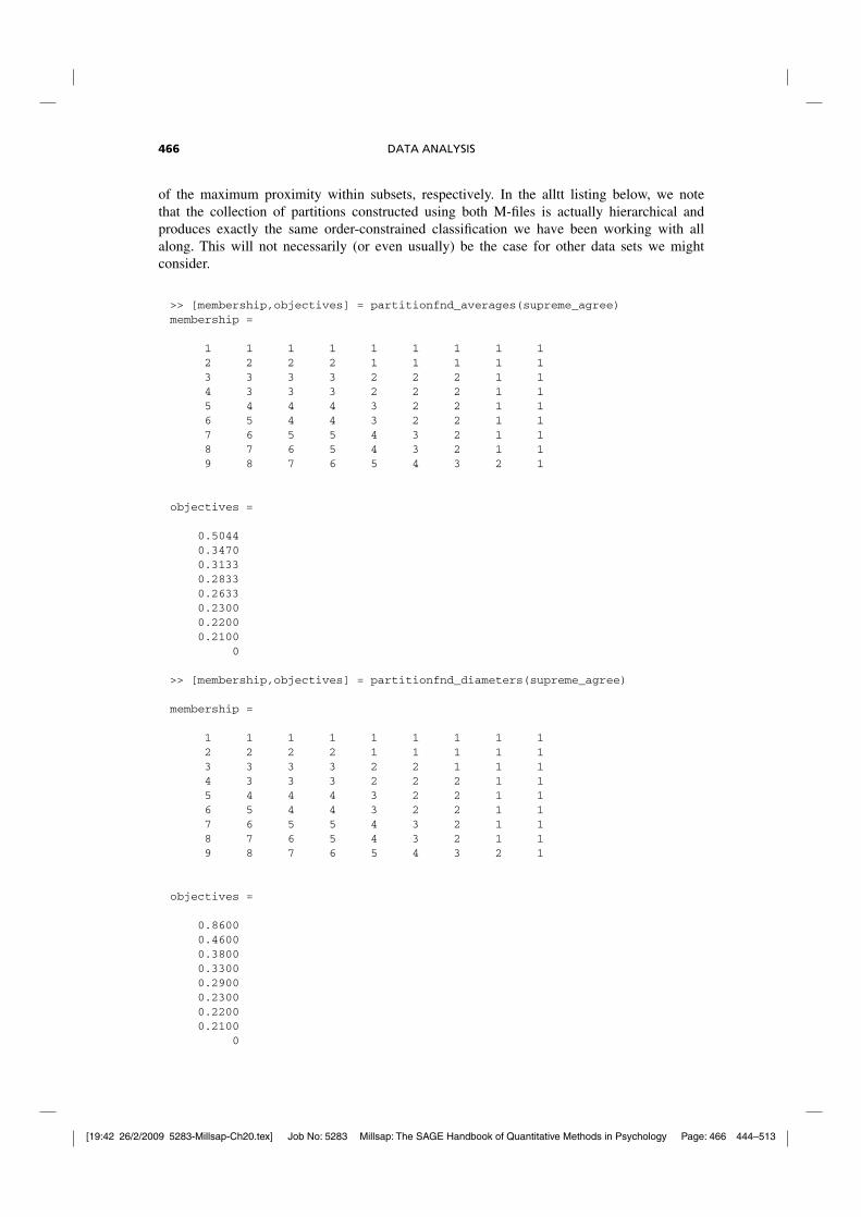
The M-files introduced below remove the requirement that the new classes in Pt are formed byuniting only existing classes in Pt−1. Although class contiguity is maintained with respect to thesame object order in the partitions identified, the requirement that the classes be nested is relaxedso that if a class is present in Pt−1, it will no longer need to appear either as a class by itselfor be properly contained within some class in Pt . The M-files for constructing the collectionof partitions respecting the given object order are called partitionfnd_averages.m andpartitionfnd_diameters, and use DP to construct a set of partitions with from 1 ton ordered classes. The criteria minimized is the maximum over clusters of the average or
[19:42 26/2/2009 5283-Millsap-Ch20.tex] Job No: 5283 Millsap: The SAGE Handbook of Quantitative Methods in Psychology Page: 466 444–513
466 DATA ANALYSIS
of the maximum proximity within subsets, respectively. In the alltt listing below, we notethat the collection of partitions constructed using both M-files is actually hierarchical andproduces exactly the same order-constrained classification we have been working with allalong. This will not necessarily (or even usually) be the case for other data sets we mightconsider.
>> [membership,objectives] = partitionfnd_averages(supreme_agree)membership =
1 1 1 1 1 1 1 1 12 2 2 2 1 1 1 1 13 3 3 3 2 2 2 1 14 3 3 3 2 2 2 1 15 4 4 4 3 2 2 1 16 5 4 4 3 2 2 1 17 6 5 5 4 3 2 1 18 7 6 5 4 3 2 1 19 8 7 6 5 4 3 2 1
objectives =
0.50440.34700.31330.28330.26330.23000.22000.2100
0
>> [membership,objectives] = partitionfnd_diameters(supreme_agree)
membership =
1 1 1 1 1 1 1 1 12 2 2 2 1 1 1 1 13 3 3 3 2 2 1 1 14 3 3 3 2 2 2 1 15 4 4 4 3 2 2 1 16 5 4 4 3 2 2 1 17 6 5 5 4 3 2 1 18 7 6 5 4 3 2 1 19 8 7 6 5 4 3 2 1
objectives =
0.86000.46000.38000.33000.29000.23000.22000.2100
0

[19:42 26/2/2009 5283-Millsap-Ch20.tex] Job No: 5283 Millsap: The SAGE Handbook of Quantitative Methods in Psychology Page: 467 444–513
CLUSTER ANALYSIS 467
AN ALTERNATIVE AND GENERALIZABLE VIEW OF ULTRAMETRIC MATRIXDECOMPOSITION
A general mechanism exists for decomposing any ultrametric matrix U into a (non-negatively)weighted sum of dichotomous (0/1) matrices, each representing one of the partitions of thehierarchy, P0, . . . ,Pn−2, induced by U (note that the conjoint partition is explicitly excluded inthese expressions for the numerical reason we allude to below). Specifically, if Pt = {p(t)
ij }, for0 ≤ t ≤ n − 2, is an n × n symmetric (0/1) dissimilarity matrix corresponding to Pt in whichan entry p(t)
ij is 0 if Oi and Oj belong to the same class in Pt and otherwise equal to 1, then forsome collection of suitably chosen non-negative weights, α0, α1, . . . , αn−2,
U =n−2∑
t=0
αtPt (9)
Generally, the non-negative weights, α0, α1, . . . , αn−2, are given by the (differences in) partitionincrements that calibrate the vertical axis of the dendrogram. Moreover, because the ultrametricrepresented by Figure 20.2 was generated by optimizing a least-squares loss function in relationto a given proximity matrix P, an alternative interpretation for the obtained weights is that theysolve the nonnegative least-squares task of
min{αt≥0, 0≤t≤n−2}∑
i<j
(pij −n−2∑
t=0
αtp(t)ij )2, (10)
for the fixed collection of dichotomous matrices P0, P1, . . . , Pn−2. Although the solution to (10)is generated indirectly in this case from the least-squares optimal ultrametric directly fitted to P, ingeneral, for any fixed proximity matrix P and collection of dichotomous matrices, P0, . . . , Pn−2,however obtained, the nonnegative weights αt , 0 ≤ t ≤ n−2, solving (10) can be obtained withany nonnegative least-squares optimization method. We will routinely use in particular (andwithout further comment) the code rewritten in MATLAB for a subroutine originally providedby Wollan and Dykstra (1987) based on a strategy for solving linear inequality constrainedleast-squares tasks called iterative projection.
In the alltt script below, the M-file, partitionfit.m, is used to reconstruct the order-constrained ultrametric for the supreme_agree data set. The crucial component is inconstructing the m×n matrix (member) that defines class membership for the m = 8 nontrivialpartitions generating the ultrametric. Note in particular that the unnecessary conjoint partitioninvolving a single class is not included (in fact, its inclusion would produce a numerical errorin the least-squares subcode integral to partitionfit.m; thus, there would be a nonzerovalue for end_condition). The M-file partitionfit.m will be relied on again whenwe further generalize the type of structural representations possible for a proximity matrix in alater section.
>> member = [1 1 1 1 2 2 2 2 2;1 1 1 1 2 2 2 3 3;1 2 2 2 3 3 3 4 4;1 2 2 2 3 4 4 5 5;
1 2 3 3 4 5 5 6 6;1 2 3 3 4 5 6 7 7;1 2 3 4 5 6 7 8 8;1 2 3 4 5 6 7
8 9]
member =
1 1 1 1 2 2 2 2 2
1 1 1 1 2 2 2 3 3
1 2 2 2 3 3 3 4 4

[19:42 26/2/2009 5283-Millsap-Ch20.tex] Job No: 5283 Millsap: The SAGE Handbook of Quantitative Methods in Psychology Page: 468 444–513
468 DATA ANALYSIS
1 2 2 2 3 4 4 5 5
1 2 3 3 4 5 5 6 6
1 2 3 3 4 5 6 7 7
1 2 3 4 5 6 7 8 8
1 2 3 4 5 6 7 8 9
>> [fitted,vaf,weights,end_condition] = partitionfit(supreme_agree,member)
fitted =
0 0.3633 0.3633 0.3633 0.6405 0.6405 0.6405 0.6405 0.6405
0.3633 0 0.2850 0.2850 0.6405 0.6405 0.6405 0.6405 0.6405
0.3633 0.2850 0 0.2200 0.6405 0.6405 0.6405 0.6405 0.6405
0.3633 0.2850 0.2200 0 0.6405 0.6405 0.6405 0.6405 0.6405
0.6405 0.6405 0.6405 0.6405 0 0.3100 0.3100 0.4017 0.4017
0.6405 0.6405 0.6405 0.6405 0.3100 0 0.2300 0.4017 0.4017
0.6405 0.6405 0.6405 0.6405 0.3100 0.2300 0 0.4017 0.4017
0.6405 0.6405 0.6405 0.6405 0.4017 0.4017 0.4017 0 0.2100
0.6405 0.6405 0.6405 0.6405 0.4017 0.4017 0.4017 0.2100 0
vaf =
0.7369
weights =
0.2388
0.0383
0.0533
0.0250
0.0550
0.0100
0.0100
0.2100
end_condition =
0
An alternative (and generalizable) graphical representation for anultrametric
Two rather distinct graphical ways for displaying an ultrametric are given in Figures 20.2 and20.3. Figure 20.2 is in the form of a traditional dendrogram (or a graph-theoretic tree) wherethe distinct ultrametric values are used to calibrate the vertical axis and indicate the level atwhich two classes are united to form a new class in a partition within the hierarchy. Each newclass formed is represented by a closed circle, and referred to as an internal node of the tree.Considering the nine justices to be the terminal nodes (represented by open circles and listedleft-to-right in the constraining order), the ultrametric value between any two objects can alsobe constructed by taking one-half of the minimum path length between the two correspondingterminal nodes (proceeding upwards from one terminal node through the internal node thatdefines the first class in the partition hierarchy containing them both, and then back down to

[19:42 26/2/2009 5283-Millsap-Ch20.tex] Job No: 5283 Millsap: The SAGE Handbook of Quantitative Methods in Psychology Page: 469 444–513
CLUSTER ANALYSIS 469
St Br Gi So Oc Ke Re Sc Th
.21
.01.01
.06
.02
.05
.04
.24
Figure 20.3 An alternative representation for the fitted values of the order-constrainedultrametric (having VAF of 73.69%).
the other terminal node, with all horizontal lengths in the tree used for graphical purposes onlyand assumed to be of length zero). Or if the vertical axis calibrations were themselves halved,the minimum path lengths would directly provide the fitted ultrametric values. There is onedistinguished node in the tree of Figure 20.2 (indicated by the biggest solid circle), referred toas the ‘root’ and with the property of being equidistant from all terminal nodes. In contrast tovarious additive tree representations to follow in later sections, the defining characteristic for anultrametric is the existence of a position on the tree equidistant from all terminal nodes.
Figure 20.3 provides an alternative representation for an ultrametric. Here, a partition ischaracterized by a set of horizontal lines each encompassing the objects in a particular class.This presentation is possible because the justices are listed from left-to-right in the same orderused to constrain the construction of the ultrametric, and thus, each class of a partition containsobjects contiguous with respect to this ordering. The calibration on the vertical axis next to eachset of horizontal lines representing a specific partition is the increment to the fitted dissimilaritybetween two particular justices if that pair is not encompassed by a continuous horizontal linefor a class in this partition. For an ultrametric, a nonnegative increment value for the partition Pt
is just αt ≥ 0 for 0 ≤ t ≤ n−2 (and noting that an increment for the trivial partition containing a

[19:42 26/2/2009 5283-Millsap-Ch20.tex] Job No: 5283 Millsap: The SAGE Handbook of Quantitative Methods in Psychology Page: 470 444–513
470 DATA ANALYSIS
single class, Pn−1, is not defined nor given in the representation of Figure 20.3). As an exampleand considering the pair (Oc,Sc), horizontal lines do not encompass this pair except for the last(nontrivial) partition P7 ; thus, the fitted ultrametric value of .40 is the sum of the incrementsattached to the partitions P0, . . . ,P6: .2100+ .0100+ .0100+ .0550+ .0250+ .0533+ .0383 =.4016(≈ .4017, to rounding).
EXTENSIONS TO ADDITIVE TREES: INCORPORATING CENTROID METRICS
A currently popular alternative to the use of a simple ultrametric in classification, and what mightbe considered an extension, is that of an additive tree. Generalizing the earlier characterizationof an ultrametric, an n × n matrix, D = {dij}, can be called an additive tree metric (matrix)if the ultrametric inequality condition is replaced by: dij + dkl ≤ max{dik + djl, dil + djk} for1 ≤ i, j, k, l ≤ n (the additive tree metric inequality). Or equivalently (and again, much moreunderstandable), for any object quadruple Oi, Oj, Ok , and Ol, the largest two values among thesums dij + dkl, dik + djl, and dil + djk are equal.
Any additive tree metric matrix D can be represented (in many ways) as a sum of two matrices,say U = {uij} and C = {cij}, where U is an ultrametric matrix, and cij = gi +gj for 1 ≤ i �= j ≤ nand cii = 0 for 1 ≤ i ≤ n, based on some set of values g1, . . . , gn. The multiplicity of suchpossible decompositions results from the choice of where to place the root in the type of graphicalrepresentation we give in Figure 20.5 (p. 000).
To eventually construct the type of graphical additive tree representation of Figure 20.5, theprocess followed is to first graph the dendrogram induced by U, where (as for any ultrametric) thechosen root is equidistant from all terminal nodes. The branches connecting the terminal nodesare then lengthened or shortened depending on the signs and absolute magnitudes of g1, . . . , gn.If one were willing to consider the (arbitrary) inclusion of a sufficiently large additive constant tothe entries in D, the values of g1, . . . , gn could be assumed nonnegative. In this case, the matrixC would represent what is called a centroid metric, and although a nicety, such a restriction isnot absolutely necessary for the extensions we pursue.
The number of ‘weights’ an additive tree metric requires could be equated to the maximumnumber of ‘branch lengths’ that a representation such as Figure 20.5 might necessitate, i.e., nbranches attached to the terminal nodes, and n − 3 to the internal nodes only, for a total of2n−3. For an ultrametric, the number of such ‘weights’ could be identified with the n−1 levelsat which the new subsets get formed in the partition hierarchy, and would represent about halfof that necessary for an additive tree. What this implies is that the VAF measures obtained forultrametrics and additive trees are not directly comparable because a very differing number of‘free weights’ must be specified for each. We are reluctant to use the word ‘parameter’ due to theabsence of any explicit statistical model and because the topology (e.g., the branching pattern)of the structures that ultimately get reified by imposing numerical values for the ‘weights’,must first be identified by some type of combinatorial optimization search process. In short,there doesn’t seem to be an unambiguous way to specify, for example, the number of estimated‘parameters’, the number of ‘degrees-of-freedom’ left over, or how to ‘adjust’ the VAF valueas we can do in multiple regression so it has an expected value of zero when there is ‘nothinggoing on’.
One of the difficulties in working with additive trees and displaying them graphically isto find some sensible spot to site a root for the tree. Depending on where the root is placed,a differing decomposition of D into an ultrametric and a centroid metric is implied. Theultrametric components induced by the choice of root can differ widely with major substantivedifferences in the branching patterns of the hierarchical clustering. The two M-files discussedbelow, cent_ultrafnd_confit.m and cent_ultrafnd_confnd.m, both identify

[19:42 26/2/2009 5283-Millsap-Ch20.tex] Job No: 5283 Millsap: The SAGE Handbook of Quantitative Methods in Psychology Page: 471 444–513
CLUSTER ANALYSIS 471
best-fitting additive trees to a given proximity matrix but where the terminal nodes of anultrametric portion of the fitted matrix are then ordered according to a constraining order(conperm) that is either input (in cent_ultrafnd_confit.m) or is identified as a goodone to use (in cent_ultrafnd_confnd.m) and then given as an output vector. In bothcases, a centroid metric is first fit to the input proximity matrix; the residual matrix is carriedover to the order-constrained ultrametric constructions routines (ultrafnd_confit.mor ultrafnd_confnd.m), and thus, the root is chosen naturally for the ultrametriccomponent. The whole process then iterates with a new centroid metric estimation, an order-constrained ultrametric re-estimation, and so on until convergence is achieved for the VAFvalues.
We illustrate below what occurs for our supreme_agree data and the imposition of theidentity permutation (1:9) for the terminal nodes of the ultrametric. The relevant outputs are theultrametric component in targtwo and the lengths for the centroid metric in lengthsone.To graph the additive tree, we first add .60 to the entries in targtwo to make them all positiveand graph this ultrametric as in Figure 20.4. Then (1/2)(.60) = .30 is subtracted from each term in
St Br Gi So Oc Ke Re Sc Th
.09
.36.37
.40
.49
.59
.73
Figure 20.4 A Dendrogram (tree) representation for the ordered-constrained ultrametriccomponent of the additive tree represented in Figure 20.5.

[19:42 26/2/2009 5283-Millsap-Ch20.tex] Job No: 5283 Millsap: The SAGE Handbook of Quantitative Methods in Psychology Page: 472 444–513
472 DATA ANALYSIS
St
BrGi
So
Oc
Ke
Re
Sc Th
.00
.10
.20
.30
.40
.50
Figure 20.5 An graph-theoretic representation for the ordered-constrained additive treedescribed in the text (having VAF of 98.41%).
lengthsone; the branches attached to the terminal nodes of the ultrametric are then stretchedor shrunk accordingly to produce Figure 20.5. These stretching/shrinking factors are as follows:St: (.07); Br: (−.05); Gi: (−.06); So: (−.09); Oc: (−.18); Ke: (−.14); Re: (−.10); Sc: (.06); Th:(.06). We note that if cent_ultrafnd_confnd.mwere invoked to find a good constrainingorder for the ultrametric component, the VAF could be increased slightly (to 98.56% from 98.41%for Figure 20.5) using the conperm of [3 1 4 2 5 6 7 9 8]. No real substantive interpretativedifference, however, is apparent from the structure given for a constraining identity permutation.
>> [find,vaf,outperm,targone,targtwo,lengthsone] = cent_ultrafnd_confit(supreme_agree,
randperm(9),1:9)
find =
0 0.3800 0.3707 0.3793 0.6307 0.6643 0.7067 0.8634 0.8649
0.3800 0 0.2493 0.2579 0.5093 0.5429 0.5852 0.7420 0.7434
0.3707 0.2493 0 0.2428 0.4941 0.5278 0.5701 0.7269 0.7283
0.3793 0.2579 0.2428 0 0.4667 0.5003 0.5427 0.6994 0.7009

[19:42 26/2/2009 5283-Millsap-Ch20.tex] Job No: 5283 Millsap: The SAGE Handbook of Quantitative Methods in Psychology Page: 473 444–513
CLUSTER ANALYSIS 473
0.6307 0.5093 0.4941 0.4667 0 0.2745 0.3168 0.4736 0.4750
0.6643 0.5429 0.5278 0.5003 0.2745 0 0.2483 0.4051 0.4065
0.7067 0.5852 0.5701 0.5427 0.3168 0.2483 0 0.3293 0.3307
0.8634 0.7420 0.7269 0.6994 0.4736 0.4051 0.3293 0 0.2100
0.8649 0.7434 0.7283 0.7009 0.4750 0.4065 0.3307 0.2100 0
vaf =
0.9841
outperm =
1 2 3 4 5 6 7 8 9
targone =
0 0.6246 0.6094 0.5820 0.4977 0.5313 0.5737 0.7304 0.7319
0.6246 0 0.4880 0.4606 0.3763 0.4099 0.4522 0.6090 0.6104
0.6094 0.4880 0 0.4454 0.3611 0.3948 0.4371 0.5939 0.5953
0.5820 0.4606 0.4454 0 0.3337 0.3673 0.4097 0.5664 0.5679
0.4977 0.3763 0.3611 0.3337 0 0.2830 0.3253 0.4821 0.4836
0.5313 0.4099 0.3948 0.3673 0.2830 0 0.3590 0.5158 0.5172
0.5737 0.4522 0.4371 0.4097 0.3253 0.3590 0 0.5581 0.5595
0.7304 0.6090 0.5939 0.5664 0.4821 0.5158 0.5581 0 0.7163
0.7319 0.6104 0.5953 0.5679 0.4836 0.5172 0.5595 0.7163 0
targtwo =
0 -0.2446 -0.2387 -0.2027 0.1330 0.1330 0.1330 0.1330 0.1330
-0.2446 0 -0.2387 -0.2027 0.1330 0.1330 0.1330 0.1330 0.1330
-0.2387 -0.2387 0 -0.2027 0.1330 0.1330 0.1330 0.1330 0.1330
-0.2027 -0.2027 -0.2027 0 0.1330 0.1330 0.1330 0.1330 0.1330
0.1330 0.1330 0.1330 0.1330 0 -0.0085 -0.0085 -0.0085 -0.0085
0.1330 0.1330 0.1330 0.1330 -0.0085 0 -0.1107 -0.1107 -0.1107
0.1330 0.1330 0.1330 0.1330 -0.0085 -0.1107 0 -0.2288 -0.2288
0.1330 0.1330 0.1330 0.1330 -0.0085 -0.1107 -0.2288 0 -0.5063
0.1330 0.1330 0.1330 0.1330 -0.0085 -0.1107 -0.2288 -0.5063 0
lengthsone =
0.3730 0.2516 0.2364 0.2090 0.1247 0.1583 0.2007 0.3574 0.3589
>> [find,vaf,outperm,targone,targtwo,lengthsone] = cent_ultrafnd_confnd(supreme_agree,
randperm(9))
find =
0 0.3400 0.2271 0.2794 0.4974 0.5310 0.5734 0.7316 0.7301
0.3400 0 0.3629 0.4151 0.6331 0.6667 0.7091 0.8673 0.8659
0.2271 0.3629 0 0.2556 0.4736 0.5072 0.5495 0.7078 0.7063
0.2794 0.4151 0.2556 0 0.4967 0.5303 0.5727 0.7309 0.7294
0.4974 0.6331 0.4736 0.4967 0 0.2745 0.3168 0.4750 0.4736
0.5310 0.6667 0.5072 0.5303 0.2745 0 0.2483 0.4065 0.4051
0.5734 0.7091 0.5495 0.5727 0.3168 0.2483 0 0.3307 0.3293

[19:42 26/2/2009 5283-Millsap-Ch20.tex] Job No: 5283 Millsap: The SAGE Handbook of Quantitative Methods in Psychology Page: 474 444–513
474 DATA ANALYSIS
0.7316 0.8673 0.7078 0.7309 0.4750 0.4065 0.3307 0 0.2100
0.7301 0.8659 0.7063 0.7294 0.4736 0.4051 0.3293 0.2100 0
vaf =
0.9856
outperm =
3 1 4 2 5 6 7 9 8
targone =
0 0.6151 0.4556 0.4787 0.3644 0.3980 0.4404 0.5986 0.5971
0.6151 0 0.5913 0.6144 0.5001 0.5337 0.5761 0.7343 0.7329
0.4556 0.5913 0 0.4549 0.3406 0.3742 0.4165 0.5748 0.5733
0.4787 0.6144 0.4549 0 0.3637 0.3973 0.4397 0.5979 0.5964
0.3644 0.5001 0.3406 0.3637 0 0.2830 0.3253 0.4836 0.4821
0.3980 0.5337 0.3742 0.3973 0.2830 0 0.3590 0.5172 0.5158
0.4404 0.5761 0.4165 0.4397 0.3253 0.3590 0 0.5595 0.5581
0.5986 0.7343 0.5748 0.5979 0.4836 0.5172 0.5595 0 0.7163
0.5971 0.7329 0.5733 0.5964 0.4821 0.5158 0.5581 0.7163 0
targtwo =
0 -0.2751 -0.2284 -0.1993 0.1330 0.1330 0.1330 0.1330 0.1330
-0.2751 0 -0.2284 -0.1993 0.1330 0.1330 0.1330 0.1330 0.1330
-0.2284 -0.2284 0 -0.1993 0.1330 0.1330 0.1330 0.1330 0.1330
-0.1993 -0.1993 -0.1993 0 0.1330 0.1330 0.1330 0.1330 0.1330
0.1330 0.1330 0.1330 0.1330 0 -0.0085 -0.0085 -0.0085 -0.0085
0.1330 0.1330 0.1330 0.1330 -0.0085 0 -0.1107 -0.1107 -0.1107
0.1330 0.1330 0.1330 0.1330 -0.0085 -0.1107 0 -0.2288 -0.2288
0.1330 0.1330 0.1330 0.1330 -0.0085 -0.1107 -0.2288 0 -0.5063
0.1330 0.1330 0.1330 0.1330 -0.0085 -0.1107 -0.2288 -0.5063 0
lengthsone =
0.2397 0.3754 0.2159 0.2390 0.1247 0.1583 0.2007 0.3589 0.3574
In addition to the additive tree identification routines just described, there are two moreillustrated below, called atreefit.m and atreefnd.m; these two M-files are directanalogues of ultrafit.m and ultrafnd.m introduced in an earlier section. Again,the complete-link target, sc_completelink_target, can be used in atreefit.m(producing a structure with VAF of 94.89%); atreefnd.m generates the same additive tree ascent_ultrafnd_confnd.m with a VAF of 98.56%. The M-file, atreedec.m, providesa mechanism for decomposing any given additive tree matrix into an ultrametric and a centroidmetric matrix (where the root is situated halfway along the longest path). The form of the usage is:
[ulmetric,ctmetric] = atreedec(prox,constant)
where prox is the input (additive tree) proximity matrix (still with a zero main diagonal anda dissimilarity interpretation); constant is a nonnegative number (less than or equal to the

[19:42 26/2/2009 5283-Millsap-Ch20.tex] Job No: 5283 Millsap: The SAGE Handbook of Quantitative Methods in Psychology Page: 475 444–513
CLUSTER ANALYSIS 475
maximum proximity value) that controls the positivity of the constructed ultrametric values;ulmetric is the ultrametric component of the decomposition; ctmetric is the centroidmetric component (given by values, g1, . . . , gn, assigned to each of the objects, some of whichmay be negative depending on the input proximity matrix and constant used).
There are two additional utility files, ultraorder.m and ultraplot.m, that may proveuseful in explaining the ultrametric components identified from an application ofatreedec.m.In the explicit usage:
[orderprox,orderperm] = ultraorder(prox)
the matrix prox is assumed to be ultrametric; orderperm is a permutation used to display anAR form in orderprox, where:
orderprox = prox(orderperm,orderperm)
The second utility’s usage of ultraplot(ultra), where ultra is a matrix presumed tosatisfy the ultrametric inequality, first adds a constant to all values in ultra to make the entriespositive; the MATLAB Statistics Toolbox routine, dendrogram.m, is then invoked to plot theresulting ultrametric matrix.
>> load supreme_agree.dat
>> load sc_completelink_target.dat
>> [fit,vaf] = atreefit(supreme_agree,sc_completelink_target)
fit =
0 0.3972 0.3850 0.3678 0.6748 0.6670 0.6756 0.8456 0.8470
0.3972 0 0.2635 0.2464 0.5533 0.5456 0.5542 0.7242 0.7256
0.3850 0.2635 0 0.2200 0.5411 0.5333 0.5419 0.7119 0.7133
0.3678 0.2464 0.2200 0 0.5239 0.5162 0.5247 0.6947 0.6962
0.6748 0.5533 0.5411 0.5239 0 0.2449 0.2535 0.4235 0.4249
0.6670 0.5456 0.5333 0.5162 0.2449 0 0.2300 0.4158 0.4172
0.6756 0.5542 0.5419 0.5247 0.2535 0.2300 0 0.4243 0.4258
0.8456 0.7242 0.7119 0.6947 0.4235 0.4158 0.4243 0 0.2100
0.8470 0.7256 0.7133 0.6962 0.4249 0.4172 0.4258 0.2100 0
vaf =
0.9489
>> [find,vaf] = atreefnd(supreme_agree,randperm(9))
find =
0 0.4151 0.3400 0.3629 0.6329 0.6668 0.7091 0.8659 0.8673
0.4151 0 0.2794 0.2556 0.4965 0.5304 0.5727 0.7295 0.7309
0.3400 0.2794 0 0.2271 0.4972 0.5311 0.5734 0.7302 0.7316
0.3629 0.2556 0.2271 0 0.4734 0.5073 0.5496 0.7064 0.7078
0.6329 0.4965 0.4972 0.4734 0 0.2745 0.3168 0.4736 0.4750
0.6668 0.5304 0.5311 0.5073 0.2745 0 0.2483 0.4051 0.4065
0.7091 0.5727 0.5734 0.5496 0.3168 0.2483 0 0.3293 0.3307
0.8659 0.7295 0.7302 0.7064 0.4736 0.4051 0.3293 0 0.2100
0.8673 0.7309 0.7316 0.7078 0.4750 0.4065 0.3307 0.2100 0

[19:42 26/2/2009 5283-Millsap-Ch20.tex] Job No: 5283 Millsap: The SAGE Handbook of Quantitative Methods in Psychology Page: 476 444–513
476 DATA ANALYSIS
vaf =
0.9856
>> [ulmetric,ctmetric] = atreedec(find,1.0)
ulmetric =
0 0.8168 0.7410 0.7877 1.1327 1.1327 1.1327 1.1327 1.1327
0.8168 0 0.8168 0.8168 1.1327 1.1327 1.1327 1.1327 1.1327
0.7410 0.8168 0 0.7877 1.1327 1.1327 1.1327 1.1327 1.1327
0.7877 0.8168 0.7877 0 1.1327 1.1327 1.1327 1.1327 1.1327
1.1327 1.1327 1.1327 1.1327 0 0.9748 0.9748 0.9748 0.9748
1.1327 1.1327 1.1327 1.1327 0.9748 0 0.8724 0.8724 0.8724
1.1327 1.1327 1.1327 1.1327 0.9748 0.8724 0 0.7543 0.7543
1.1327 1.1327 1.1327 1.1327 0.9748 0.8724 0.7543 0 0.4768
1.1327 1.1327 1.1327 1.1327 0.9748 0.8724 0.7543 0.4768 0
ctmetric =
-0.1327
-0.2691
-0.2684
-0.2922
-0.3671
-0.3332
-0.2909
-0.1341
-0.1327
>> [orderprox,orderperm] = ultraorder(ulmetric)
orderprox =
0 0.7877 0.7877 0.8168 1.1327 1.1327 1.1327 1.1327 1.1327
0.7877 0 0.7410 0.8168 1.1327 1.1327 1.1327 1.1327 1.1327
0.7877 0.7410 0 0.8168 1.1327 1.1327 1.1327 1.1327 1.1327
0.8168 0.8168 0.8168 0 1.1327 1.1327 1.1327 1.1327 1.1327
1.1327 1.1327 1.1327 1.1327 0 0.7543 0.7543 0.8724 0.9748
1.1327 1.1327 1.1327 1.1327 0.7543 0 0.4768 0.8724 0.9748
1.1327 1.1327 1.1327 1.1327 0.7543 0.4768 0 0.8724 0.9748
1.1327 1.1327 1.1327 1.1327 0.8724 0.8724 0.8724 0 0.9748
1.1327 1.1327 1.1327 1.1327 0.9748 0.9748 0.9748 0.9748 0
orderperm =
4 3 1 2 7 8 9 6 5
SOME BIBLIOGRAPHIC COMMENTS
There are a number of book-length presentations of cluster analysis methods available(encompassing differing collections of subtopics within the field). We list several of the betterones to consult in the reference section to follow, and note these here in chronological order:

[19:42 26/2/2009 5283-Millsap-Ch20.tex] Job No: 5283 Millsap: The SAGE Handbook of Quantitative Methods in Psychology Page: 477 444–513
CLUSTER ANALYSIS 477
Anderberg (1973); Hartigan (1975); Späth (1980); Barthélemy and Guénoche (1991); Mirkin(1996); Arabie, Hubert, and DeSoete (1996); Everitt and Rabe-Hesketh (1997); Gordon (1999).The items that would be closest to the approaches taken here with MATLAB and the emphasison least-squares, would be the monograph by Hubert, Arabie, and Meulman (2006), and thereview articles by Hubert, Köhn, and Steinley (in press); and Steinley and Hubert (2008).
ULTRAMETRIC EXTENSIONS BY FITTING PARTITIONS CONTAININGCONTIGUOUS SUBSETS
The M-file, partitionfit.m, is a very general routine giving a least-squares approximationto a proximity matrix based on a given collection of partitions. Thus, no matter how the set ofcandidate partitions might be chosen, a least-squares fitted matrix to the given proximity matrixis achieved. For example, if we simply use the nested partitions constructed from an ultrametric,the ultrametric would be retrieved when the latter is used as the input proximity matrix. Inthis section, we show how partitionfit.m can also be used to select partitions from apredefined set (this selection is done by those partitions assigned strictly positive weights) thatmight serve to reconstruct the proximity matrix well. The M-file, consec_subsetfit.m,defines (n(n − 1)/2) − 1 candidate partitions each characterized by a single contiguous clusterof objects, with all objects before and after this contiguous set forming individual clusters ofthe partition (the minus 1 appears in the count due to the (conjoint) partition defined by asingle contiguous set being excluded). The M-file, consec_subsetfit_alter.m, variesthe specific definition of the partitions by including all objects before and all objects after thecontiguous set (when nonempty) as separate individual clusters of the partitions.
As can be seen from the alltt output provided below, the nonnegative weighted partitions fromconsec_subsetfit.m, producing a fitted matrix with VAF of 92.61%, are as follows:
Partition Partition increment
{{St,Br,Gi,So},{Oc},{Ke},{Re},{Sc},{Th}} .1939{{St,Br,Gi,So,Oc},{Ke},{Re},{Sc},{Th}} .0300{{St,Br,Gi,So,Oc,Ke},{Re},{Sc},{Th}} .0389{{St,Br,Gi,So,Oc,Ke,Re},{Sc},{Th}} .1315{{St},{Br,Gi,So,Oc,Ke,Re,Sc,Th}} .1152
{{St},{Br},{Gi,So,Oc,Ke,Re,Sc,Th}} .0052{{St},{Br},{Gi},{So,Oc,Ke,Re,Sc,Th}} .0153
{{St},{Br},{Gi},{So},{Oc,Ke,Re,Sc,Th}} .2220{{St},{Br},{Gi},{So},{Oc},{Ke,Re,Sc,Th}} .0633
{{St},{Br},{Gi},{So},{Oc},{Ke},{Re,Sc,Th}} .0030
Similarly, we have a very high VAF of 98.12% based on the more numerous partitions generatedfrom consec_subsetfit_alter.m:
>> load supreme_agree.dat
>> [fitted,vaf,weights,end_condition,member] = consec_subsetfit(supreme_agree);
>> fitted
fitted =
0 0.4239 0.4239 0.4239 0.6178 0.6478 0.6866 0.8181 0.8181
0.4239 0 0.3087 0.3087 0.5026 0.5326 0.5715 0.7029 0.7029
0.4239 0.3087 0 0.3035 0.4974 0.5274 0.5663 0.6977 0.6977
0.4239 0.3087 0.3035 0 0.4821 0.5121 0.5510 0.6824 0.6824
0.6178 0.5026 0.4974 0.4821 0 0.2901 0.3290 0.4604 0.4604
0.6478 0.5326 0.5274 0.5121 0.2901 0 0.2657 0.3972 0.3972
0.6866 0.5715 0.5663 0.5510 0.3290 0.2657 0 0.3942 0.3942

[19:42 26/2/2009 5283-Millsap-Ch20.tex] Job No: 5283 Millsap: The SAGE Handbook of Quantitative Methods in Psychology Page: 478 444–513
478 DATA ANALYSIS
Partition Partition increment
{{St,Br},{Gi,So,Oc,Ke,Re,Sc,Th}} .0021{{St,Br,Gi},{So,Oc,Ke,Re,Sc,Th}} .0001{{St,Br,Gi,So},{Oc,Ke,Re,Sc,Th}} .0001{{St,Br,Gi,So,Oc,Ke},{Re,Sc,Th}} .0100{{St,Br,Gi,So,Oc,Ke,Re},{Sc,Th}} .1218
{{St},{Br,Gi},{So,Oc,Ke,Re,Sc,Th}} .0034{{St},{Br,Gi,So,Oc},{Ke,Re,Sc,Th}} .0056{{St},{Br,Gi,So,Oc,Ke,Re},{Sc,Th}} .0113{{St},{Br,Gi,So,Oc,Ke,Re,Sc},{Th}} .0038{{St},{Br,Gi,So,Oc,Ke,Re,Sc,Th}} .1170
{{St,Br},{Gi,So},{Oc,Ke,Re,Sc,Th}} .0165{{St,Br},{Gi,So,Oc,Ke,Re,Sc,Th}} .0095
{{St,Br,Gi},{So,Oc},{Ke,Re,Sc,Th}} .0197{{St,Br,Gi},{So,Oc,Ke,Re,Sc,Th}} .0115{{St,Br,Gi,So},{Oc,Ke,Re,Sc,Th}} .2294{{St,Br,Gi,So,Oc},{Ke,Re,Sc,Th}} .0353{{St,Br,Gi,So,Oc,Ke},{Re,Sc,Th}} .0400{{St,Br,Gi,So,Oc,Ke,Re},{Sc,Th}} .0132
{{St},{Br},{Gi},{So},{Oc},{Ke},{Re},{Sc},{Th}} .2050
0.8181 0.7029 0.6977 0.6824 0.4604 0.3972 0.3942 0 0.3942
0.8181 0.7029 0.6977 0.6824 0.4604 0.3972 0.3942 0.3942 0
>> vaf
vaf =
0.9261
>> weights
weights =
0
0
0.1939
0.0300
0.0389
0.1315
0
0
0
0
0
0
0
0.1152
0
0
0
0
0
0.0052
0
0
0
0
0.0153

[19:42 26/2/2009 5283-Millsap-Ch20.tex] Job No: 5283 Millsap: The SAGE Handbook of Quantitative Methods in Psychology Page: 479 444–513
CLUSTER ANALYSIS 479
0
0
0
0.2220
0
0
0.0633
0
0.0030
0
0
>> end_condition
end_condition =
0
>> member
member =
1 1 3 4 5 6 7 8 9
1 1 1 4 5 6 7 8 9
1 1 1 1 5 6 7 8 9
1 1 1 1 1 6 7 8 9
1 1 1 1 1 1 7 8 9
1 1 1 1 1 1 1 8 9
1 1 1 1 1 1 1 1 9
1 2 2 4 5 6 7 8 9
1 2 2 2 5 6 7 8 9
1 2 2 2 2 6 7 8 9
1 2 2 2 2 2 7 8 9
1 2 2 2 2 2 2 8 9
1 2 2 2 2 2 2 2 9
1 2 2 2 2 2 2 2 2
1 2 3 3 5 6 7 8 9
1 2 3 3 3 6 7 8 9
1 2 3 3 3 3 7 8 9
1 2 3 3 3 3 3 8 9
1 2 3 3 3 3 3 3 9
1 2 3 3 3 3 3 3 3
1 2 3 4 4 6 7 8 9
1 2 3 4 4 4 7 8 9
1 2 3 4 4 4 4 8 9
1 2 3 4 4 4 4 4 9
1 2 3 4 4 4 4 4 4
1 2 3 4 5 5 7 8 9
1 2 3 4 5 5 5 8 9
1 2 3 4 5 5 5 5 9
1 2 3 4 5 5 5 5 5
1 2 3 4 5 6 6 8 9
1 2 3 4 5 6 6 6 9
1 2 3 4 5 6 6 6 6
1 2 3 4 5 6 7 7 9
1 2 3 4 5 6 7 7 7
1 2 3 4 5 6 7 8 8
1 2 3 4 5 6 7 8 9

[19:42 26/2/2009 5283-Millsap-Ch20.tex] Job No: 5283 Millsap: The SAGE Handbook of Quantitative Methods in Psychology Page: 480 444–513
480 DATA ANALYSIS
>> [fitted,vaf,weights,end_condition,member] = consec_subsetfit_alter(supreme_agree)
fitted =
0 0.3460 0.3740 0.4053 0.6347 0.6700 0.7200 0.8550 0.8550
0.3460 0 0.2330 0.2677 0.4971 0.5380 0.5880 0.7342 0.7380
0.3740 0.2330 0 0.2396 0.4855 0.5264 0.5764 0.7227 0.7264
0.4053 0.2677 0.2396 0 0.4509 0.5114 0.5614 0.7076 0.7114
0.6347 0.4971 0.4855 0.4509 0 0.2655 0.3155 0.4617 0.4655
0.6700 0.5380 0.5264 0.5114 0.2655 0 0.2550 0.4012 0.4050
0.7200 0.5880 0.5764 0.5614 0.3155 0.2550 0 0.3512 0.3550
0.8550 0.7342 0.7227 0.7076 0.4617 0.4012 0.3512 0 0.2087
0.8550 0.7380 0.7264 0.7114 0.4655 0.4050 0.3550 0.2087 0
vaf =
0.9812
weights =
0.0021
0.0001
0.0001
0
0.0100
0.1218
0
0.0034
0
0.0056
0
0.0113
0.0038
0.1170
0.0165
0
0
0
0
0.0095
0.0197
0
0
0
0.0115
0
0
0
0.2294
0
0
0.0353
0
0.0400
0.0132
0.2050

[19:42 26/2/2009 5283-Millsap-Ch20.tex] Job No: 5283 Millsap: The SAGE Handbook of Quantitative Methods in Psychology Page: 481 444–513
CLUSTER ANALYSIS 481
end_condition =
0
member =
1 1 9 9 9 9 9 9 9
1 1 1 9 9 9 9 9 9
1 1 1 1 9 9 9 9 9
1 1 1 1 1 9 9 9 9
1 1 1 1 1 1 9 9 9
1 1 1 1 1 1 1 9 9
1 1 1 1 1 1 1 1 9
1 2 2 9 9 9 9 9 9
1 2 2 2 9 9 9 9 9
1 2 2 2 2 9 9 9 9
1 2 2 2 2 2 9 9 9
1 2 2 2 2 2 2 9 9
1 2 2 2 2 2 2 2 9
1 2 2 2 2 2 2 2 2
1 1 3 3 9 9 9 9 9
1 1 3 3 3 9 9 9 9
1 1 3 3 3 3 9 9 9
1 1 3 3 3 3 3 9 9
1 1 3 3 3 3 3 3 9
1 1 3 3 3 3 3 3 3
1 1 1 4 4 9 9 9 9
1 1 1 4 4 4 9 9 9
1 1 1 4 4 4 4 9 9
1 1 1 4 4 4 4 4 9
1 1 1 4 4 4 4 4 4
1 1 1 1 5 5 9 9 9
1 1 1 1 5 5 5 9 9
1 1 1 1 5 5 5 5 9
1 1 1 1 5 5 5 5 5
1 1 1 1 1 6 6 9 9
1 1 1 1 1 6 6 6 9
1 1 1 1 1 6 6 6 6
1 1 1 1 1 1 7 7 9
1 1 1 1 1 1 7 7 7
1 1 1 1 1 1 1 8 8
1 2 3 4 5 6 7 8 9
To see how well one might do by choosing only eight partitions (i.e., the same numberneeded to define the order-constrained best-fitting ultrametric), the single (disjoint) partitiondefined by nine separate classes is chosen in both instances, plus the seven partitions havingthe highest assigned positive weights. For those picked from the partition pool identifiedby consec_subsetfit.m, the VAF drops slightly from 92.61% to 92.51% based on thepartitions:
Partition Partition increment
{{St,Br,Gi,So},{Oc},{Ke},{Re},{Sc},{Th}} .1923{{St,Br,Gi,So,Oc},{Ke},{Re},{Sc},{Th}} .0301{{St,Br,Gi,So,Oc,Ke},{Re},{Sc},{Th}} .0396{{St,Br,Gi,So,Oc,Ke,Re},{Sc},{Th}} .1316

[19:42 26/2/2009 5283-Millsap-Ch20.tex] Job No: 5283 Millsap: The SAGE Handbook of Quantitative Methods in Psychology Page: 482 444–513
482 DATA ANALYSIS
{{St},{Br,Gi,So,Oc,Ke,Re,Sc,Th}} .1224{{St},{Br},{Gi},{So},{Oc,Ke,Re,Sc,Th}} .2250
{{St},{Br},{Gi},{So},{Oc},{Ke,Re,Sc,Th}} .0671{{St},{Br},{Gi},{So},{Oc},{Ke},{Re},{Sc},{Th}} .0000
For those selected from the set generated by consec_subsetfit_alter.m, the VAF againdrops slightly from 98.12% to 97.97%. But in some absolute sense given the size of the VAF,the eight partitions listed below seem to be about all that can be extracted from this particularjustice data set.
Partition Partition increment
{{St,Br,Gi,So,Oc,Ke,Re},{Sc,Th}} .1466{{St},{Br,Gi,So,Oc,Ke,Re,Sc,Th}} .1399
{{St,Br},{Gi,So},{Oc,Ke,Re,Sc,Th}} .0287{{St,Br,Gi},{So,Oc},{Ke,Re,Sc,Th}} .0326{{St,Br,Gi,So},{Oc,Ke,Re,Sc,Th}} .2269{{St,Br,Gi,So,Oc},{Ke,Re,Sc,Th}} .0316{{St,Br,Gi,So,Oc,Ke},{Re,Sc,Th}} .0500
{{St},{Br},{Gi},{So},{Oc},{Ke},{Re},{Sc},{Th}} .2051
The three highest weighted partitions have very clear interpretations: {Sc,Th} versus therest; {St} versus the rest; {St,Br,Gi,So} as the left versus {Oc,Ke,Re,Sc,Th} as the right.The few remaining partitions revolve around several other less salient (adjacent) objectpairings that are also very interpretable in relation to the object ordering from liberal toconservative. We give a graphical representation for this latter culled collection of partitionsin Figure 20.6. Again, the partition increments are not included in a fitted value whenevera continuous horizontal line encompasses the relevant objects in a defining cluster of thepartition.
>> member = [1 1 1 1 5 6 7 8 9;1 1 1 1 1 6 7 8 9;1 1 1 1 1 1 7 8 9;1 1 1 1 1 1 1 8 9;
1 2 2 2 2 2 2 2 2;1 2 3 4 5 5 5 5 5;1 2 3 4 5 6 6 6 6;1 2 3 4 5 6 7 8 9]
member =
1 1 1 1 5 6 7 8 9
1 1 1 1 1 6 7 8 9
1 1 1 1 1 1 7 8 9
1 1 1 1 1 1 1 8 9
1 2 2 2 2 2 2 2 2
1 2 3 4 5 5 5 5 5
1 2 3 4 5 6 6 6 6
1 2 3 4 5 6 7 8 9
>> [fitted,vaf,weights,end_condition] = partitionfit(supreme_agree,member)
fitted =
0 0.4245 0.4245 0.4245 0.6168 0.6469 0.6865 0.8181 0.8181
0.4245 0 0.3021 0.3021 0.4944 0.5245 0.5641 0.6957 0.6957
0.4245 0.3021 0 0.3021 0.4944 0.5245 0.5641 0.6957 0.6957
0.4245 0.3021 0.3021 0 0.4944 0.5245 0.5641 0.6957 0.6957
0.6168 0.4944 0.4944 0.4944 0 0.2895 0.3291 0.4607 0.4607
0.6469 0.5245 0.5245 0.5245 0.2895 0 0.2620 0.3936 0.3936
0.6865 0.5641 0.5641 0.5641 0.3291 0.2620 0 0.3936 0.3936
0.8181 0.6957 0.6957 0.6957 0.4607 0.3936 0.3936 0 0.3936
0.8181 0.6957 0.6957 0.6957 0.4607 0.3936 0.3936 0.3936 0

[19:42 26/2/2009 5283-Millsap-Ch20.tex] Job No: 5283 Millsap: The SAGE Handbook of Quantitative Methods in Psychology Page: 483 444–513
CLUSTER ANALYSIS 483
St Br Gi So Oc Ke Re Sc Th
.21
.23
.15
.14
.05
.03
.03
.03
Figure 20.6 A representation for the fitted values of the (generalized) structure described inthe text (having VAF of 97.97%).
vaf =
0.9251
weights =
0.1923
0.0301
0.0396
0.1316
0.1224
0.2350
0.0671
0
end_condition =
0
>> member = [1 1 1 1 1 1 1 9 9;1 2 2 2 2 2 2 2 2;1 1 3 3 9 9 9 9 9;1 1 1 4 4 9 9 9 9;
1 1 1 1 5 5 5 5 5;1 1 1 1 1 6 6 6 6;1 1 1 1 1 1 7 7 7;1 2 3 4 5 6 7 8 9]

[19:42 26/2/2009 5283-Millsap-Ch20.tex] Job No: 5283 Millsap: The SAGE Handbook of Quantitative Methods in Psychology Page: 484 444–513
484 DATA ANALYSIS
member =
1 1 1 1 1 1 1 9 9
1 2 2 2 2 2 2 2 2
1 1 3 3 9 9 9 9 9
1 1 1 4 4 9 9 9 9
1 1 1 1 5 5 5 5 5
1 1 1 1 1 6 6 6 6
1 1 1 1 1 1 7 7 7
1 2 3 4 5 6 7 8 9
>> [fitted,vaf,weights,end_condition] = partitionfit(supreme_agree,member)
fitted =
0 0.3450 0.3736 0.4062 0.6331 0.6647 0.7147 0.8613 0.8613
0.3450 0 0.2337 0.2664 0.4933 0.5248 0.5748 0.7215 0.7215
0.3736 0.2337 0 0.2377 0.4933 0.5248 0.5748 0.7215 0.7215
0.4062 0.2664 0.2377 0 0.4606 0.5248 0.5748 0.7215 0.7215
0.6331 0.4933 0.4933 0.4606 0 0.2693 0.3193 0.4659 0.4659
0.6647 0.5248 0.5248 0.5248 0.2693 0 0.2551 0.4017 0.4017
0.7147 0.5748 0.5748 0.5748 0.3193 0.2551 0 0.3517 0.3517
0.8613 0.7215 0.7215 0.7215 0.4659 0.4017 0.3517 0 0.2051
0.8613 0.7215 0.7215 0.7215 0.4659 0.4017 0.3517 0.2051 0
vaf =
0.9797
weights =
0.1466
0.1399
0.0287
0.0326
0.2269
0.0316
0.0500
0.2051
end_condition =
0
ULTRAMETRICS AND ADDITIVE TREES FOR TWO-MODE(RECTANGULAR) PROXIMITY DATA
The proximity data considered thus far for obtaining some type of structure, such as an ultrametricor an additive tree, have been assumed to be on one intact set of objects, S = {O1, . . . , On},and complete in the sense that proximity values are present between all object pairs. Supposenow that the available proximity data are two-mode, and between two distinct object sets,SA = {O1A, . . . , OnaA} and SB = {O1B, . . . , OnbB}, containing na and nb objects, respectively,given by an na × nb proximity matrix Q = {qrs}. Again, we assume that the entries in Q are

[19:42 26/2/2009 5283-Millsap-Ch20.tex] Job No: 5283 Millsap: The SAGE Handbook of Quantitative Methods in Psychology Page: 485 444–513
CLUSTER ANALYSIS 485
keyed as dissimilarities, and a joint structural representation is desired for the combined setSA ∪ SB. We might caution at the outset of the need to have legitimate proximities to makethe analyses to follow very worthwhile or interpretable. There are many numerical elicitationschemes where subjects (e.g., raters) are asked to respond to some set of objects (e.g., items).If the elicitation is for, say, preference, then proximity may be a good interpretation for thenumerical values. If, on the other hand, the numerical value is merely a rating given on somemore-or-less objective criterion where only errors of observation induce the variability fromrater to rater, then probably not.
Conditions have been proposed in the literature for when the entries in a matrix fitted to Qcharacterize an ultrametric or an additive tree representation. In particular, suppose an na × nb
matrix, F = {frs}, is fitted to Q through least squares subject to the constraints that follow:Ultrametric (Furnas, 1980): for all distinct object quadruples, OrA, OsA, OrB, OsB, where OrA,
OsA ∈ SA and OrB, OsB, ∈ SB, and considering the entries in F corresponding to the pairs, (OrA,OrB), (OrA, OsB), (OsA OrB), and (OsA, OsB), say frArB , frAsB , fsArB , fsAsB , respectively, the largesttwo must be equal.
Additive trees (Brossier, 1987): for all distinct object sextuples, OrA, OsA, OtA, OrB, OsB,OtB, where OrA, OsA, OtA ∈ SA and OrB, OsB, OtB, ∈ SB, and considering the entries in Fcorresponding to the pairs (OrA, OrB), (OrA, OsB), (OrA, OtB), (OsA, OrB), (OsA, OsB), (OsA, OtB),(OtA, OrB), (OtA, OsB), and (OtA, OtB), say frArB , frAsB , frAtB , fsArB , fsAsB , fsAtB , ftArB , ftAsB , ftAtB ,respectively, the largest two of the following sums must be equal:
frArB + fsAsB + ftAtB
frArB + fsAtB + ftAsB
frAsB + fsArB + ftAtB
frAsB + fsAtB + ftArB
frAtB + fsArB + ftAsB
frAtB + fsAsB + ftArB
Two-mode ultrametrics
To illustrate the fitting of a given two-mode ultrametric, a two-mode target is generated by extract-ing a 5 × 4 portion from the 9 × 9 ultrametric target matrix, sc_completelink_target,used earlier. This file has contents as follows (sc_completelink_target5x4.dat):
0.3800 0.3800 0.8600 0.86000.2900 0.2200 0.8600 0.86000.8600 0.8600 0.3300 0.46000.8600 0.8600 0.2300 0.46000.8600 0.8600 0.4600 0.2100
The five rows correspond to the judges, St, Gi, Oc, Re, Th; the four columns to Br,So, Ke, Sc. As the two-mode 5 × 4 proximity matrix, the appropriate portion of thesupreme_agree proximity matrix will be used in the fitting process; the corresponding fileis called supreme_agree5x4.dat, with contents:
0.3000 0.3700 0.6400 0.86000.2800 0.2200 0.5100 0.72000.4500 0.4500 0.3300 0.46000.5700 0.5600 0.2300 0.34000.7600 0.7100 0.4100 0.2100

[19:42 26/2/2009 5283-Millsap-Ch20.tex] Job No: 5283 Millsap: The SAGE Handbook of Quantitative Methods in Psychology Page: 486 444–513
486 DATA ANALYSIS
Because of the way the joint set of row and columns objects is numbered, the five rows arelabeled from 1 to 5 and the four columns from 6 to 9. Thus, the correspondence between thejustices and the numbers obviously differs from earlier applications:
1:St; 2:Gi; 3:Oc; 4:Re; 5:Th; 6:Br; 7:So; 8:Ke; 9:Sc
The M-file, ultrafittm.m, fits a given ultrametric to a two-mode proximity matrix, and hasusage:
[fit,vaf] = ultrafittm(proxtm,targ)
where proxtm is the two-mode (rectangular) input proximity matrix (with a dissimilarityinterpretation); targ is an ultrametric matrix of the same size as proxtm; fitis the least-squares optimal matrix (with variance-accounted-for of vaf) to proxtmsatisfying the two-mode ultrametric constraints implicit in targ. An example follows usingsc_completelink_target5x4 for targ and supreme_agree5x4 as proxtm:
>> load supreme_agree5x4.dat
>> load sc_completelink_target5x4.dat
>> supreme_agree5x4
supreme_agree5x4 =
0.3000 0.3700 0.6400 0.86000.2800 0.2200 0.5100 0.72000.4500 0.4500 0.3300 0.46000.5700 0.5600 0.2300 0.34000.7600 0.7100 0.4100 0.2100
>> sc_completelink_target5x4
sc_completelink_target5x4 =
0.3800 0.3800 0.8600 0.86000.2900 0.2200 0.8600 0.86000.8600 0.8600 0.3300 0.46000.8600 0.8600 0.2300 0.46000.8600 0.8600 0.4600 0.2100
>> [fit,vaf] = ultrafittm(supreme_agree5x4,sc_completelink_target5x4)
fit =
0.3350 0.3350 0.6230 0.62300.2800 0.2200 0.6230 0.62300.6230 0.6230 0.3300 0.40330.6230 0.6230 0.2300 0.40330.6230 0.6230 0.4033 0.2100
vaf =
0.7441

[19:42 26/2/2009 5283-Millsap-Ch20.tex] Job No: 5283 Millsap: The SAGE Handbook of Quantitative Methods in Psychology Page: 487 444–513
CLUSTER ANALYSIS 487
A VAF of 74.41% was obtained for the fitted ultrametric; the easily interpretable hierarchy isgiven below with indications of when the partitions were formed using both the number andletter schemes to label the justices:
Partition Level
{{4:Re,8:Ke,3:Oc,5:Th,9:Sc,1:St,2:Gi,7:So,6:Br} .6230{{4:Re,8:Ke,3:Oc,5:Th,9:Sc},{1:St,2:Gi,7:So,6:Br}} .4033{{4:Re,8:Ke,3:Oc},{5:Th,9:Sc},{1:St,2:Gi,7:So,6:Br} .3350
{{4:Re,8:Ke,3:Oc},{5:Th,9:Sc},{1:St},{2:Gi,7:So,6:Br}} .3300{{4:Re,8:Ke},{3:Oc},{5:Th,9:Sc},{1:St},{2:Gi,7:So,6:Br}} .2800
{{4:Re,8:Ke},{3:Oc},{5:Th,9:Sc},{1:St},{2:Gi,7:So},{6:Br}} .2300{{4:Re},{8:Ke},{3:Oc},{5:Th,9:Sc},{1:St},{2:Gi,7:So},{6:Br}} .2200
{{4:Re},{8:Ke},{3:Oc},{5:Th,9:Sc},{1:St},{2:Gi},{7:So},{6:Br}} .2100{{4:Re},{8:Ke},{3:Oc},{5:Th},{9:Sc},{1:St},{2:Gi},{7:So},{6:Br}} —
The M-file, ultrafndtm.m locates a best-fitting two-mode ultrametric with usage
[find,vaf] = ultrafndtm(proxtm,inpermrow,inpermcol)
where proxtm is the two-mode input proximity matrix (with a dissimilarity interpretation);inpermrow and inpermcol are permutations for the row and column objects that determinethe order in which the inequality constraints are considered; find is the found least-squares matrix (with variance-accounted-for of vaf) to proxtm satisfying the ultrametricconstraints.The example below forsupreme_agree5x4 (using random permutations for bothinpermrow and inpermcol), finds exactly the same ultrametric as above with vaf of .7441.
>> [find,vaf] = ultrafndtm(supreme_agree5x4,randperm(5),randperm(4))
find =
0.3350 0.3350 0.6230 0.62300.2800 0.2200 0.6230 0.62300.6230 0.6230 0.3300 0.40330.6230 0.6230 0.2300 0.40330.6230 0.6230 0.4033 0.2100
vaf =
0.7441
Two-mode additive trees
The identification of a best-fitting two-mode additive tree will be done somewhat differentlythan for a two-mode ultrametric representation, largely because of future storage considerationswhen huge matrices might be considered. Specifically, a (two-mode) centroid metric and a (two-mode) ultrametric matrix will be identified so that their sum is a good-fitting two-mode additivetree. Because a centroid metric can be obtained in closed-form, we first illustrate the fittingof just a centroid metric to a two-mode proximity matrix with the M-file, centfittm.m. Itsusage is of the form:
[fit,vaf,lengths] = centfittm(proxtm)
giving the least-squares fitted two-mode centroid metric (fit) to proxtm, the two-mode rectangular input proximity matrix (with a dissimilarity interpretation). The n values

[19:42 26/2/2009 5283-Millsap-Ch20.tex] Job No: 5283 Millsap: The SAGE Handbook of Quantitative Methods in Psychology Page: 488 444–513
488 DATA ANALYSIS
[where n = number of rows (na) + number of columns (nb)] serve to define the approximatingsums, ur +vs, where the ur are for the na rows and the vs for the nb columns; these ur and vs valuesare given in the vector lengths of size n×1, with row values first followed by the column val-ues. The closed-form formula used for ur (or vs) can be given simply as the rth row (or sth column)mean of proxtm minus one-half the grand mean. In the example below using the two-modematrix,supreme_agree5x4, a two-mode centroid metric by itself has a (paltry)vafof .1090.
>> [fit,vaf,lengths] = centfittm(supreme_agree5x4)
fit =
0.5455 0.5355 0.4975 0.59150.4355 0.4255 0.3875 0.48150.4255 0.4155 0.3775 0.47150.4280 0.4180 0.3800 0.47400.5255 0.5155 0.4775 0.5715
vaf =
0.1090
lengths =
0.30800.19800.18800.19050.28800.23750.22750.18950.2835
The identification of a two-mode additive tree with the M-file, atreefndtm.m, proceedsiteratively.Atwo-mode centroid metric is first found and the original two-mode proximity matrixresidualized; a two-mode ultrametric is then identified for the residual matrix. The process repeatswith the centroid and ultrametric components alternatingly being refit until a small change inthe overall VAF occurs. The M-file has the explicit usage:
[find,vaf,ultra,lengths] = ... atreefndtm(proxtm,inpermrow,inpermcol)
Here, proxtm is the rectangular input proximity matrix (with a dissimilarity interpretation);inpermrow and inpermcol are permutations for the row and column objects that determinethe order in which the inequality constraints are considered; find is the found least-squaresmatrix (with variance-accounted-for of vaf) to proxtm satisfying the two-mode additive treeconstraints. The vector lengths contains the row followed by column values for the two-modecentroid metric component; ultra is the ultrametric component. In the example given below,the identified two-mode additive-tree for supreme_agree5x4 has vaf of .9953. The actualpartition hierarchy is given in the next section along with an indication of when the variouspartitions are formed using a utility M-file that completes a two-mode ultrametric so it is definedover the entire joint set.
>> [find,vaf,ultra,lengths] = atreefndtm(supreme_agree5x4,randperm(5),randperm(4))

[19:42 26/2/2009 5283-Millsap-Ch20.tex] Job No: 5283 Millsap: The SAGE Handbook of Quantitative Methods in Psychology Page: 489 444–513
CLUSTER ANALYSIS 489
find =
0.3000 0.3768 0.6533 0.8399
0.2732 0.2200 0.5251 0.7117
0.4625 0.4379 0.3017 0.4883
0.5755 0.5510 0.2333 0.3400
0.7488 0.7243 0.4067 0.2100
vaf =
0.9953
ultra =
-0.2658 -0.1644 0.1576 0.1576
-0.1644 -0.1931 0.1576 0.1576
0.1576 0.1576 0.0668 0.0668
0.1576 0.1576 -0.1145 -0.1945
0.1576 0.1576 -0.1145 -0.4978
lengths =
0.3368
0.2086
0.0759
0.1889
0.3623
0.2290
0.2045
0.1589
0.3456
Completing a two-mode ultrametric to one defined on the combinedobject set
Instead of relying only on our general intuition (and problem-solving skills) to transform a fittedtwo-mode ultrametric to one we could interpret directly as a sequence of partitions for the jointset SA∪SB, the M-file,ultracomptm.m, provides the explicit completion of a given two-modeultrametric matrix to a symmetric proximity matrix (defined on SA ∪ SB and satisfying the usualultrametric constraints). Thus, this completion, in effect, estimates the (missing) ultrametricvalues that must be present between objects from the same cluster and from the same mode. Thegeneral syntax has the form:
[ultracomp] = ultracomptm(ultraproxtm)
where ultraproxtm is the na × nb fitted two-mode ultrametric matrix; ultracomp isthe completed n × n proximity matrix having the usual ultrametric pattern for the completeobject set of size n = na + nb. As seen in the example below, the use of ultrafndtm.mon supreme_agree5x4, and the subsequent application of ultracomptm.m (plusultraorder.m on ultracomp), leads directly to the partition hierarchy given followingthe alltt output.
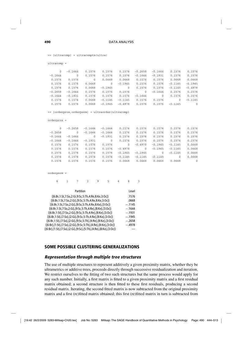
[19:42 26/2/2009 5283-Millsap-Ch20.tex] Job No: 5283 Millsap: The SAGE Handbook of Quantitative Methods in Psychology Page: 490 444–513
490 DATA ANALYSIS
>> [ultracomp] = ultracomptm(ultra)
ultracomp =
0 -0.1644 0.1576 0.1576 0.1576 -0.2658 -0.1644 0.1576 0.1576
-0.1644 0 0.1576 0.1576 0.1576 -0.1644 -0.1931 0.1576 0.1576
0.1576 0.1576 0 0.0668 0.0668 0.1576 0.1576 0.0668 0.0668
0.1576 0.1576 0.0668 0 -0.1945 0.1576 0.1576 -0.1145 -0.1945
0.1576 0.1576 0.0668 -0.1945 0 0.1576 0.1576 -0.1145 -0.4978
-0.2658 -0.1644 0.1576 0.1576 0.1576 0 -0.1644 0.1576 0.1576
-0.1644 -0.1931 0.1576 0.1576 0.1576 -0.1644 0 0.1576 0.1576
0.1576 0.1576 0.0668 -0.1145 -0.1145 0.1576 0.1576 0 -0.1145
0.1576 0.1576 0.0668 -0.1945 -0.4978 0.1576 0.1576 -0.1145 0
>> [orderprox,orderperm] = ultraorder(ultracomp)
orderprox =
0 -0.2658 -0.1644 -0.1644 0.1576 0.1576 0.1576 0.1576 0.1576
-0.2658 0 -0.1644 -0.1644 0.1576 0.1576 0.1576 0.1576 0.1576
-0.1644 -0.1644 0 -0.1931 0.1576 0.1576 0.1576 0.1576 0.1576
-0.1644 -0.1644 -0.1931 0 0.1576 0.1576 0.1576 0.1576 0.1576
0.1576 0.1576 0.1576 0.1576 0 -0.4978 -0.1945 -0.1145 0.0668
0.1576 0.1576 0.1576 0.1576 -0.4978 0 -0.1945 -0.1145 0.0668
0.1576 0.1576 0.1576 0.1576 -0.1945 -0.1945 0 -0.1145 0.0668
0.1576 0.1576 0.1576 0.1576 -0.1145 -0.1145 -0.1145 0 0.0668
0.1576 0.1576 0.1576 0.1576 0.0668 0.0668 0.0668 0.0668 0
orderperm =
6 1 7 2 9 5 4 8 3
Partition Level
{{6:Br,1:St,7:So,2:Gi,9:Sc,5:Th,4:Re,8:Ke,3:Oc}} .1576{{6:Br,1:St,7:So,2:Gi},{9:Sc,5:Th,4:Re,8:Ke,3:Oc}} .0668
{{6:Br,1:St,7:So,2:Gi},{9:Sc,5:Th,4:Re,8:Ke},{3:Oc}} −.1145{{6:Br,1:St,7:So,2:Gi},{9:Sc,5:Th,4:Re},{8:Ke},{3:Oc}} −.1644
{{6:Br,1:St},{7:So,2:Gi},{9:Sc,5:Th,4:Re},{8:Ke},{3:Oc}} −.1931{{6:Br,1:St},{7:So},{2:Gi},{9:Sc,5:Th,4:Re},{8:Ke},{3:Oc}} −.1945
{{6:Br,1:St},{7:So},{2:Gi},{9:Sc,5:Th},{4:Re},{8:Ke},{3:Oc}} −.2658{{6:Br},{1:St},{7:So},{2:Gi},{9:Sc,5:Th},{4:Re},{8:Ke},{3:Oc}} −.4978
{{6:Br},{1:St},{7:So},{2:Gi},{9:Sc},{5:Th},{4:Re},{8:Ke},{3:Oc}} —
SOME POSSIBLE CLUSTERING GENERALIZATIONS
Representation through multiple tree structures
The use of multiple structures to represent additively a given proximity matrix, whether they beultrametrics or additive trees, proceeds directly through successive residualization and iteration.We restrict ourselves to the fitting of two such structures but the same process would apply forany such number. Initially, a first matrix is fitted to a given proximity matrix and a first residualmatrix obtained; a second structure is then fitted to these first residuals, producing a secondresidual matrix. Iterating, the second fitted matrix is now subtracted from the original proximitymatrix and a first (re)fitted matrix obtained; this first (re)fitted matrix in turn is subtracted from

[19:42 26/2/2009 5283-Millsap-Ch20.tex] Job No: 5283 Millsap: The SAGE Handbook of Quantitative Methods in Psychology Page: 491 444–513
CLUSTER ANALYSIS 491
the original proximity matrix and a new second matrix (re)fitted. This process continues untilthe vaf for the sum of both fitted matrices no longer changes substantially.
The M-files, biultrafnd.m and biatreefnd.m fit (additively) two ultrametric oradditive tree matrices in the least-squares sense. The explicit usages are:
[find,vaf,targone,targtwo] = biultrafnd(prox,inperm)
[find,vaf,targone,targtwo] = biatreefnd(prox,inperm)
where prox is the given input proximity matrix (with a zero main diagonal and a dissimilarityinterpretation); inperm is a permutation that determines the order in which the inequalityconstraints are considered (and thus can be made random to search for different locally optimalrepresentations); find is the obtained least-squares matrix (with variance-accounted-for ofvaf) to prox, and is the sum of the two ultrametric or additive tree matrices targone andtargtwo.
We will not given an explicit illustration of using two fitted structures to represent a proximitymatrix. The data set we have been using, supreme_agree, is not a good example for multiplestructures because only one such device is really needed to explain everything present in thedata. More suitable proximity matrices would probably themselves be obtained by a mixture oraggregation of other proximity matrices, reflecting somewhat different underlying structures;hopefully, these could be “teased apart” in an analysis using multiple additive structures.
Individual differences and ultrametrics
One aspect of the given M-files introduced in earlier sections but not emphasized, is theirpossible use in the confirmatory context of fitting individual differences. Explicitly, we beginwith a collection of, say, N proximity matrices, P1, . . . , PN , obtained from N separate sources,and through some weighting and averaging process, construct a single aggregate proximitymatrix, PA. On the basis of PA, suppose an ultrametric or additive tree is constructed; we labelthe latter the “common space” consistent with what is usually done in the (weighted) Euclideanmodel in multidimensional scaling. Each of the N proximity matrices then can be used in aconfirmatory fitting of an ultrametric (with, say, ultrafit.m) or an additive tree (with, say,atreefit.m). A very general “subject/private space” is generated for each source and wherethe branch lengths are unique to that source, subject only to the topology (branching) constraintsof the group space. In effect, we would be carrying out an individual differences analysis by usinga “deviation from the mean” philosophy. A group structure is first identified in an exploratorymanner from an aggregate proximity matrix; the separate matrices that went into the aggregateare then fit in a confirmatory way, one-by-one. There does not seem to be any particular apriori advantage in trying to carry out this process “all at once”; to the contrary, the simplicityof the deviation approach and its immediate generalizability to a variety of possible structuralrepresentations, holds out the hope of greater substantive interpretability.
Incorporating transformations of the proximities
In the use of either a one- or two-mode proximity matrix, the data were assumed ‘as is’, andwithout any preliminary transformation. It was noted that some analyses leading to negativevalues might be more pleasingly interpretable if they were positive, and thus, a sufficiently largeadditive constant was imposed on the original proximities (without any real loss of generality).In other words, the structures fit to proximity matrices have an invariance with respect to lineartransformations of the proximities. A second type of transformation is implicit in the use of

[19:42 26/2/2009 5283-Millsap-Ch20.tex] Job No: 5283 Millsap: The SAGE Handbook of Quantitative Methods in Psychology Page: 492 444–513
492 DATA ANALYSIS
additive trees where a centroid (metric), fit as part of the whole representational structure, hasthe effect of double-centering (i.e., for the input proximity matrix deviated from the centroid,zero sums are present within rows or columns). In effect, the analysis methods iterate betweenfitting an ultrametric and a centroid, attempting to squeeze out every last bit of VAF. Maybe amore direct strategy (and one that would most likely not affect the substantive interpretationsmaterially) would be to initially double-center (either a one- or two-mode matrix), and thentreat the later to the analyses we wish to carry out, without again revisiting the double-centeringoperation during the iterative process.
A more serious consideration of proximity transformation would involve monotonicfunctions of the type familiar in nonmetric multidimensional scaling. We provide two utilities,proxmon.m and proxmontm.m, that will allow the user a chance to experiment with thesemore general transformations for both one- and two-mode proximity matrices. The usage issimilar for both M-files in providing a monotonically transformed proximity matrix that isclosest in a least-squares sense to a given (usually the structurally fitted) matrix:
[monproxpermut,vaf,diff] = proxmon(proxpermut,fitted)[monproxpermuttm,vaf,diff] = proxmontm(proxpermuttm,fittedtm)
Here, proxpermut (proxpermuttm) is the input proximity matrix (which may have beensubjected to an initial row/column permutation, hence the suffix permut), and fitted(fittedtm) is a given target matrix (typically the representational matrix such as theidentified ultrametric); the output matrix,monproxpermut (monproxpermuttm), is closestto fitted (fittedtm) in a least-squares sense and obeys the order constraints obtained fromeach pair of entries in (the upper-triangular portion of) proxpermut or proxpermuttm.As usual, vaf denotes “variance-accounted-for” but here indicates how much variance inmonproxpermut (monproxpermuttm) can be accounted for by fitted (fittedtm);finally,diff is the value of the least-squares loss function and is one-half the squared differencesbetween the entries in fitted (fittedtm) and monproxpermut (monproxpermuttm).
A script M-file is listed in the alltt output below that gives an application of proxmon.musing the best-fitting ultrametric structure found for supreme_agree. First, ultrafnd.mis invoked to obtain a fitted matrix (fit) with vaf of .7369; proxmon.m then generatesthe monotonically transformed proximity matrix (monproxpermut) with vaf of .9264 anddiff of .0622. The strategy is repeated one-hundred times (i.e., finding a fitted matrix basedon the monotonically transformed proximity matrix, finding a new monotonically transformedmatrix, and so on). To avoid degeneracy (where all matrices would just converge to zeros), thesum of squares of the fitted matrix is normalized (and held constant). Here, a perfect vaf of1.0 is achieved (and a diff of 0.0); the structure of the proximities is now pretty flattenedwith only four new clusters explicitly identified in the partition hierarchy (the levels at whichthese are formed are given next to the clusters): (Sc,Th): .2149; (Gi,So): .2251; (Ke,Re): .2353;(Br,Gi,So): .2916. Another way of stating this is to observe that the monotonically transformedproximity matrix has only five distinct values, and over 86% are at a common value of .5588,the level at which the single all-inclusive subset is formed.
>> type ultra_monotone_test
load supreme_agree.dat [fit,vaf] = ultrafnd(supreme_agree,randperm(9))
[monprox,vaf,diff] = proxmon(supreme_agree,fit)
sumfitsq = sum(sum(fit.ˆ2));
for i = 1:100

[19:42 26/2/2009 5283-Millsap-Ch20.tex] Job No: 5283 Millsap: The SAGE Handbook of Quantitative Methods in Psychology Page: 493 444–513
CLUSTER ANALYSIS 493
[fit,vaf] = ultrafit(monprox,fit);
sumnewfitsq = sum(sum(fit.ˆ2));
fit = sqrt(sumfitsq)*(fit/sumnewfitsq);
[monprox,vaf,diff] = proxmon(supreme_agree,fit);
end
fit
vaf
diff
monprox
supreme_agree
>> ultra_monotone_test
fit =
0 0.3633 0.3633 0.3633 0.6405 0.6405 0.6405 0.6405 0.6405
0.3633 0 0.2850 0.2850 0.6405 0.6405 0.6405 0.6405 0.6405
0.3633 0.2850 0 0.2200 0.6405 0.6405 0.6405 0.6405 0.6405
0.3633 0.2850 0.2200 0 0.6405 0.6405 0.6405 0.6405 0.6405
0.6405 0.6405 0.6405 0.6405 0 0.3100 0.3100 0.4017 0.4017
0.6405 0.6405 0.6405 0.6405 0.3100 0 0.2300 0.4017 0.4017
0.6405 0.6405 0.6405 0.6405 0.3100 0.2300 0 0.4017 0.4017
0.6405 0.6405 0.6405 0.6405 0.4017 0.4017 0.4017 0 0.2100
0.6405 0.6405 0.6405 0.6405 0.4017 0.4017 0.4017 0.2100 0
vaf =
0.7369
monprox =
0 0.3761 0.3633 0.3761 0.6405 0.6405 0.6405 0.6405 0.6405
0.3761 0 0.2850 0.2850 0.5211 0.6405 0.6405 0.6405 0.6405
0.3633 0.2850 0 0.2200 0.6405 0.6405 0.6405 0.6405 0.6405
0.3761 0.2850 0.2200 0 0.5211 0.6405 0.6405 0.6405 0.6405
0.6405 0.5211 0.6405 0.5211 0 0.3558 0.3100 0.5211 0.5211
0.6405 0.6405 0.6405 0.6405 0.3558 0 0.2300 0.4017 0.4017
0.6405 0.6405 0.6405 0.6405 0.3100 0.2300 0 0.3761 0.3558
0.6405 0.6405 0.6405 0.6405 0.5211 0.4017 0.3761 0 0.2100
0.6405 0.6405 0.6405 0.6405 0.5211 0.4017 0.3558 0.2100 0
vaf =
0.9264

[19:42 26/2/2009 5283-Millsap-Ch20.tex] Job No: 5283 Millsap: The SAGE Handbook of Quantitative Methods in Psychology Page: 494 444–513
494 DATA ANALYSIS
diff =
0.0622
fit =
0 0.5588 0.5588 0.5588 0.5588 0.5588 0.5588 0.5588 0.5588
0.5588 0 0.2916 0.2916 0.5588 0.5588 0.5588 0.5588 0.5588
0.5588 0.2916 0 0.2251 0.5588 0.5588 0.5588 0.5588 0.5588
0.5588 0.2916 0.2251 0 0.5588 0.5588 0.5588 0.5588 0.5588
0.5588 0.5588 0.5588 0.5588 0 0.5588 0.5588 0.5588 0.5588
0.5588 0.5588 0.5588 0.5588 0.5588 0 0.2353 0.5588 0.5588
0.5588 0.5588 0.5588 0.5588 0.5588 0.2353 0 0.5588 0.5588
0.5588 0.5588 0.5588 0.5588 0.5588 0.5588 0.5588 0 0.2149
0.5588 0.5588 0.5588 0.5588 0.5588 0.5588 0.5588 0.2149 0
vaf =
1
diff =
0
monprox =
0 0.5588 0.5588 0.5588 0.5588 0.5588 0.5588 0.5588 0.5588
0.5588 0 0.2916 0.2916 0.5588 0.5588 0.5588 0.5588 0.5588
0.5588 0.2916 0 0.2251 0.5588 0.5588 0.5588 0.5588 0.5588
0.5588 0.2916 0.2251 0 0.5588 0.5588 0.5588 0.5588 0.5588
0.5588 0.5588 0.5588 0.5588 0 0.5588 0.5588 0.5588 0.5588
0.5588 0.5588 0.5588 0.5588 0.5588 0 0.2353 0.5588 0.5588
0.5588 0.5588 0.5588 0.5588 0.5588 0.2353 0 0.5588 0.5588
0.5588 0.5588 0.5588 0.5588 0.5588 0.5588 0.5588 0 0.2149
0.5588 0.5588 0.5588 0.5588 0.5588 0.5588 0.5588 0.2149 0
supreme_agree =
0 0.3800 0.3400 0.3700 0.6700 0.6400 0.7500 0.8600 0.8500
0.3800 0 0.2800 0.2900 0.4500 0.5300 0.5700 0.7500 0.7600
0.3400 0.2800 0 0.2200 0.5300 0.5100 0.5700 0.7200 0.7400
0.3700 0.2900 0.2200 0 0.4500 0.5000 0.5600 0.6900 0.7100
0.6700 0.4500 0.5300 0.4500 0 0.3300 0.2900 0.4600 0.4600
0.6400 0.5300 0.5100 0.5000 0.3300 0 0.2300 0.4200 0.4100
0.7500 0.5700 0.5700 0.5600 0.2900 0.2300 0 0.3400 0.3200
0.8600 0.7500 0.7200 0.6900 0.4600 0.4200 0.3400 0 0.2100
0.8500 0.7600 0.7400 0.7100 0.4600 0.4100 0.3200 0.2100 0
Finding and fitting best ultrametrics in the presence of missing proximities
The various M-files discussed thus far have required proximity matrices to be complete inthe sense of having all entries present. This was true even for the two-mode case where

[19:42 26/2/2009 5283-Millsap-Ch20.tex] Job No: 5283 Millsap: The SAGE Handbook of Quantitative Methods in Psychology Page: 495 444–513
CLUSTER ANALYSIS 495
Table 20.5 Dissimilarities among ten supreme court justices for the 2005/06 term.The missing entry between O’Connor and Alito is represented with an asterisk.
St So Br Gi Oc Ke Ro Sc Al Th
1 St .00 .28 .32 .31 .43 .62 .74 .70 .87 .762 So .28 .00 .17 .36 .14 .50 .61 .64 .64 .753 Br .32 .17 .00 .36 .29 .57 .56 .59 .65 .704 Gi .31 .36 .36 .00 .43 .47 .52 .61 .59 .725 Oc .43 .14 .29 .43 .00 .43 .33 .29 * .436 Ke .62 .50 .57 .47 .43 .00 .29 .35 .13 .417 Ro .74 .61 .56 .52 .33 .29 .00 .12 .09 .188 Sc .70 .64 .59 .61 .29 .35 .12 .00 .22 .169 Al .87 .64 .65 .59 * .13 .09 .22 .00 .17
10 Th .76 .75 .70 .72 .43 .41 .18 .16 .17 .00
the between-set proximities are assumed available although all within-set proximities werenot. Three different M-files are mentioned here (analog of order.m, ultrafit.m, andultrafnd.m) allowing some of the proximities in a symmetric matrix to be absent. Themissing proximities are identified in an input matrix, proxmiss, having the same size as theinput proximity matrix, prox, but otherwise the syntaxes are the same as earlier:
[outperm,rawindex,allperms,index] = ...order_missing(prox,targ,inperm,kblock,proxmiss)
[fit,vaf] = ultrafit_missing(prox,targ,proxmiss)
[find,vaf] = ultrafnd_missing(prox,inperm,proxmiss)
The proxmiss matrix guides the search and fitting process so the missing data are ignoredwhenever they should be considered in some kind of comparison. Typically, there will be enoughother data available that this really doesn’t pose any difficulty.
As an illustration of the M-files just introduced, Table 20.5 provides data on the ten SupremeCourt justices present at some point during the 2005/06 term, and the percentage of timesjustices disagreed in non-unanimous decisions during the year. (These data were in the NewYork Times on 2 July 2006, as part of a “first-page, above-the-fold” article bylined by LindaGreenhouse entitled “Roberts Is at Court’s Helm, But He Isn’t Yet in Control”.) There is asingle missing value in the table between O’Connor (Oc) and Alito (Al) because they shareda common seat for the term until Alito’s confirmation by Congress. Roberts (Ro) served thefull year as Chief Justice so no missing data entries involve him. As can be seen in the allttoutput to follow, an empirically obtained ordering (presumably from “left” to “right”) usingorder_missing.m is:
1 : St � 4 : Gi � 3 : Br � 2 : So � 5 : Oc � 6 : Ke � 7 : Ro � 8 : Sc � 9 : Al � 10 : Th
suggesting rather strongly that Kennedy will most likely now occupy the middle position(although possibly shifted somewhat to the right) once O’Connor is removed from the court’sdeliberations. The best-fitting ultrametric obtained with ultrafnd_missing.m has VAFof 72.75%, and is given below in partition hierarchy form using the justice ordering fromorder_missing.m, except for the slight interchange of Sc and Al (this allows the fittedultrametric to display its perfect AR form, as the alltt output shows).
>> load supreme_agree_2005_6.dat

[19:42 26/2/2009 5283-Millsap-Ch20.tex] Job No: 5283 Millsap: The SAGE Handbook of Quantitative Methods in Psychology Page: 496 444–513
496 DATA ANALYSIS
>> load supreme_agree_2005_6_missing.dat
>> supreme_agree_2005_6
supreme_agree_2005_6 =
0 0.2800 0.3200 0.3100 0.4300 0.6200 0.7400 0.7000 0.8700 0.7600
0.2800 0 0.1700 0.3600 0.1400 0.5000 0.6100 0.6400 0.6400 0.7500
0.3200 0.1700 0 0.3600 0.2900 0.5700 0.5600 0.5900 0.6500 0.7000
0.3100 0.3600 0.3600 0 0.4300 0.4700 0.5200 0.6100 0.5900 0.7200
0.4300 0.1400 0.2900 0.4300 0 0.4300 0.3300 0.2900 0 0.4300
0.6200 0.5000 0.5700 0.4700 0.4300 0 0.2900 0.3500 0.1300 0.4100
0.7400 0.6100 0.5600 0.5200 0.3300 0.2900 0 0.1200 0.0900 0.1800
0.7000 0.6400 0.5900 0.6100 0.2900 0.3500 0.1200 0 0.2200 0.1600
0.8700 0.6400 0.6500 0.5900 0 0.1300 0.0900 0.2200 0 0.1700
0.7600 0.7500 0.7000 0.7200 0.4300 0.4100 0.1800 0.1600 0.1700 0
>> supreme_agree_2005_6_missing
supreme_agree_2005_6_missing =
0 1 1 1 1 1 1 1 1 1
1 0 1 1 1 1 1 1 1 1
1 1 0 1 1 1 1 1 1 1
1 1 1 0 1 1 1 1 1 1
1 1 1 1 0 1 1 1 0 1
1 1 1 1 1 0 1 1 1 1
1 1 1 1 1 1 0 1 1 1
1 1 1 1 1 1 1 0 1 1
1 1 1 1 0 1 1 1 0 1
1 1 1 1 1 1 1 1 1 0
>> [outperm,rawindex,allperms,index] = ...
order_missing(supreme_agree_2005_6,targlin(10),randperm(10),3,supreme_agree_2005_
6_missing);
>> outperm
outperm =
10 9 8 7 6 5 2 3 4 1
>> [find,vaf] = ultrafnd_missing(supreme_agree_2005_6,randperm(10),supreme_agree_2005_
6_missing)
find =
0 0.3633 0.3633 0.3100 0.3633 0.5954 0.5954 0.5954 0.5954 0.5954
0.3633 0 0.2300 0.3633 0.1400 0.5954 0.5954 0.5954 0.5954 0.5954
0.3633 0.2300 0 0.3633 0.2300 0.5954 0.5954 0.5954 0.5954 0.5954
0.3100 0.3633 0.3633 0 0.3633 0.5954 0.5954 0.5954 0.5954 0.5954
0.3633 0.1400 0.2300 0.3633 0 0.5954 0.5954 0.5954 0 0.5954
0.5954 0.5954 0.5954 0.5954 0.5954 0 0.2950 0.2950 0.2950 0.2950
0.5954 0.5954 0.5954 0.5954 0.5954 0.2950 0 0.1725 0.0900 0.1725
0.5954 0.5954 0.5954 0.5954 0.5954 0.2950 0.1725 0 0.1725 0.1600
0.5954 0.5954 0.5954 0.5954 0 0.2950 0.0900 0.1725 0 0.1725
0.5954 0.5954 0.5954 0.5954 0.5954 0.2950 0.1725 0.1600 0.1725 0

[19:42 26/2/2009 5283-Millsap-Ch20.tex] Job No: 5283 Millsap: The SAGE Handbook of Quantitative Methods in Psychology Page: 497 444–513
CLUSTER ANALYSIS 497
vaf =
0.7275
>> find([1 4 3 2 5 6 7 9 8 10],[1 4 3 2 5 6 7 9 8 10])
ans =
0 0.3100 0.3633 0.3633 0.3633 0.5954 0.5954 0.5954 0.5954 0.5954
0.3100 0 0.3633 0.3633 0.3633 0.5954 0.5954 0.5954 0.5954 0.5954
0.3633 0.3633 0 0.2300 0.2300 0.5954 0.5954 0.5954 0.5954 0.5954
0.3633 0.3633 0.2300 0 0.1400 0.5954 0.5954 0.5954 0.5954 0.5954
0.3633 0.3633 0.2300 0.1400 0 0.5954 0.5954 0 0.5954 0.5954
0.5954 0.5954 0.5954 0.5954 0.5954 0 0.2950 0.2950 0.2950 0.2950
0.5954 0.5954 0.5954 0.5954 0.5954 0.2950 0 0.0900 0.1725 0.1725
0.5954 0.5954 0.5954 0.5954 0 0.2950 0.0900 0 0.1725 0.1725
0.5954 0.5954 0.5954 0.5954 0.5954 0.2950 0.1725 0.1725 0 0.1600
0.5954 0.5954 0.5954 0.5954 0.5954 0.2950 0.1725 0.1725 0.1600 0
Partition Level
{{1:St,4:Gi,3:Br,2:So,5:Oc,6:Ke,7:Ro,9:Al,8:Sc,10:Th}} .5954{{1:St,4:Gi,3:Br,2:So,5:Oc},{6:Ke,7:Ro,9:Al,8:Sc,10:Th}} .3633
{{1:St,4:Gi},{3:Br,2:So,5:Oc},{6:Ke,7:Ro,9:Al,8:Sc,10:Th}} .3100{{1:St},{4:Gi},{3:Br,2:So,5:Oc},{6:Ke,7:Ro,9:Al,8:Sc,10:Th}} .2950
{{1:St},{4:Gi},{3:Br,2:So,5:Oc},{6:Ke},{7:Ro,9:Al,8:Sc,10:Th}} .2300{{1:St},{4:Gi},{3:Br},{2:So,5:Oc},{6:Ke},{7:Ro,9:Al,8:Sc,10:Th}} .1725
{{1:St},{4:Gi},{3:Br},{2:So,5:Oc},{6:Ke},{7:Ro,9:Al},{8:Sc,10:Th}} .1600{{1:St},{4:Gi},{3:Br},{2:So,5:Oc},{6:Ke},{7:Ro,9:Al},{8:Sc},{10:Th}} .1400
{{1:St},{4:Gi},{3:Br},{2:So},{5:Oc},{6:Ke},{7:Ro,9:Al},{8:Sc},{10:Th}} .0900{{1:St},{4:Gi},{3:Br},{2:So},{5:Oc},{6:Ke},{7:Ro},{9:Al},{8:Sc},{10:Th}} —
REFERENCES
Anderberg, M. (1973) Cluster Analysis for Applications. New York: Academic Press.Arabie, P., Hubert, L. and DeSoete, G. (eds.) (1996) Clustering and Classification. River Edge, NJ: World Scientific.Barth elemy, J-P. and Gu enoche, A. (1991) Trees and Proximity Representations. Chichester, UK: Wiley.Brossier, G. (1987) ‘Etude des matrices de proximit e rectangulaires en vue de la classification [A study of rectangular
proximity matrices from the point of view of classification]’, Revue de Statistiques Appliquees, (35) 4: 43–68.Everitt, B.S. and Rabe-Hesketh, S. (1997) The Analysis of Proximity Data. New York: Wiley.Furnas, G.W. (1980) ‘Objects and their features: The metric representation of two class data.’ Unpublished doctoral
dissertation: Stanford University.Gordon, A.D. (1999) Classification. London: Chapman and Hall/CRC.Hartigan, J. (1975) Clustering Algorithms. New York: Wiley.Hubert, L., Arabie, P. and Meulman, J. (2006) The Structural Representation of Proximity Matrices with MATLAB.
ASA-SIAM Series on Statistics and Applied Probability. Philadelphia: SIAM.Hubert, L., Köhn, H-F. and Steinley, D. (in press) ‘Order-constrained proximity matrix representations: ultrametric
generalizations and constructions with MATLAB,’ in Kolenikov, S., Steinley, D. and Thombs, L. (eds.), MethodologicalDevelopments of Statistics in the Social Sciences. New York: Wiley.
Mirkin, B. (1996) Mathematical Classification and Clustering. Dordrecht: Kluwer.Späth, H. (1980) Cluster Analysis Algorithms. Chichester, UK: Ellis Horwood.Steinley, D. and Hubert, L. (2008) ‘Order constrained solutions in K-means clustering: even better than being globally
optimal’, Psychometrika, 73: 647–664.Wollan, P.C. and Dykstra, R.L. (1987) ‘Minimizing linear inequality constrained Mahalanobis distances’, Applied
Statistics, 36: 234–240.

[19:42 26/2/2009 5283-Millsap-Ch20.tex] Job No: 5283 Millsap: The SAGE Handbook of Quantitative Methods in Psychology Page: 498 444–513
498 DATA ANALYSIS
APPENDIX A. HEADER COMMENTS FOR THE M-FILES MENTIONED IN THE TEXTOR USED INTERNALLY BY OTHER M-FILES; GIVEN IN ALPHABETICAL ORDER
arobfit.m
function [fit, vaf] = arobfit(prox, inperm)
% AROBFIT fits an anti-Robinson matrix using iterative projection to% a symmetric proximity matrix in the $L_{2}$-norm.%% syntax: [fit, vaf] = arobfit(prox, inperm)%% PROX is the input proximity matrix ($n \times n$ with a zero main% diagonal and a dissimilarity interpretation);% INPERM is a given permutation of the first $n$ integers;% FIT is the least-squares optimal matrix (with variance-% accounted-for of VAF) to PROX having an anti-Robinson form for% the row and column object ordering given by INPERM.
arobfnd.m
function [find, vaf, outperm] = arobfnd(prox, inperm, kblock)
% AROBFND finds and fits an anti-Robinson% matrix using iterative projection to% a symmetric proximity matrix in the $L_{2}$-norm based on a% permutation identified through the use of iterative quadratic% assignment.%% syntax: [find, vaf, outperm] = arobfnd(prox, inperm, kblock)%% PROX is the input proximity matrix ($n \times n$ with a zero main% diagonal and a dissimilarity interpretation);% INPERM is a given starting permutation of the first $n$ integers;% FIND is the least-squares optimal matrix (with% variance-accounted-for of VAF) to PROX having an anti-Robinson% form for the row and column object ordering given by the ending% permutation OUTPERM. KBLOCK defines the block size in the use of the% iterative quadratic assignment routine.
atreedec.m
function [ulmetric,ctmetric] = atreedec(prox,constant)
% ATREEDEC decomposes a given additive tree matrix into an% ultrametric and a centroid metric matrix (where the root is% halfway along the longest path).%% syntax: [ulmetric,ctmetric] = atreedec(prox,constant)%% PROX is the input proximity matrix (with a zero main diagonal% and a dissimilarity interpretation);% CONSTANT is a nonnegative number (less than or equal to the% maximum proximity value) that controls the% positivity of the constructed ultrametric values;% ULMETRIC is the ultrametric component of the decomposition;

[19:42 26/2/2009 5283-Millsap-Ch20.tex] Job No: 5283 Millsap: The SAGE Handbook of Quantitative Methods in Psychology Page: 499 444–513
CLUSTER ANALYSIS 499
% CTMETRIC is the centroid metric component of the decomposition% (given by values $g_{1},...,g_{n}$ for each of the objects,% some of which may actually be negative depending on the input% proximity matrix used).
atreefit.m
function [fit,vaf] = atreefit(prox,targ)
% ATREEFIT fits a given additive tree using iterative projection to% a symmetric proximity matrix in the $L_{2}$-norm.%% syntax: [fit,vaf] = atreefit(prox,targ)%% PROX is the input proximity matrix (with a zero main diagonal% and a dissimilarity interpretation);% TARG is a matrix of the same size as PROX with entries% satisfying the four-point additive tree constraints;% FIT is the least-squares optimal matrix (with% variance-accounted-for of VAF) to PROX satisfying the% additive tree constraints implicit in TARG.
atreefnd.m
function [find,vaf] = atreefnd(prox,inperm)
% ATREEFND finds and fits an additive tree using iterative projection% heuristically on a symmetric proximity matrix in the $L_{2}$-norm.%% syntax: [find,vaf] = atreefnd(prox,inperm)%% PROX is the input proximity matrix (with a zero main diagonal% and a dissimilarity interpretation);% INPERM is a permutation that determines the order in which the% inequality constraints are considered;% FIND is the found least-squares matrix (with variance-accounted-for% of VAF) to PROX satisfying the additive tree constraints.
atreefndtm.m
function [find,vaf,ultra,lengths] = ...atreefndtm(proxtm,inpermrow,inpermcol)
% ATREEFNDTM finds and fits a two-mode additive tree;% iterative projection is used% heuristically to find a two-mode ultrametric component that% is added to a two-mode centroid metric to% produce the two-mode additive tree.%% syntax: [find,vaf,ultra,lengths] = ...% atreefndtm(proxtm,inpermrow,inpermcol)%% PROXTM is the input proximity matrix% (with a dissimilarity interpretation);

[19:42 26/2/2009 5283-Millsap-Ch20.tex] Job No: 5283 Millsap: The SAGE Handbook of Quantitative Methods in Psychology Page: 500 444–513
500 DATA ANALYSIS
% INPERMROW and INPERMCOL are permutations for the row and column% objects that determine the order in which the% inequality constraints are considered;% FIND is the found least-squares matrix (with variance-accounted-for% of VAF) to PROXTM satisfying the additive tree constraints;% the vector LENGTHS contains the row followed by column values for% the two-mode centroid metric component;% ULTRA is the ultrametric component.
biatreefnd.m
function [find,vaf,targone,targtwo] = biatreefnd(prox,inperm)
% BIATREEFND finds and fits the sum% of two additive trees using iterative projection% heuristically on a symmetric proximity matrix in the $L_{2}$-norm.%% syntax: [find,vaf,targone,targtwo] = biatreefnd(prox,inperm)%% PROX is the input proximity matrix (with a zero main diagonal% and a dissimilarity interpretation);% INPERM is a permutation that determines the order in which the% inequality constraints are considered;% FIND is the found least-squares matrix (with variance-accounted-for% of VAF) to PROX and is the sum of% the two additive tree matrices TARGONE and TARGTWO.
biultrafnd.m
function [find,vaf,targone,targtwo] = biultrafnd(prox,inperm)
% BIULTRAFND finds and fits the sum% of two ultrametrics using iterative projection% heuristically on a symmetric proximity matrix in the $L_{2}$-norm.%% syntax: [find,vaf,targone,targtwo] = biultrafnd(prox,inperm)%% PROX is the input proximity matrix (with a zero main diagonal% and a dissimilarity interpretation);% INPERM is a permutation that determines the order in which the% inequality constraints are considered;% FIND is the found least-squares matrix (with variance-accounted-for% of VAF) to PROX and is the sum% of the two ultrametric matrices TARGONE and TARGTWO.
cent_ultrafnd_confit.m
function [find,vaf,outperm,targone,targtwo,lengthsone] = ...cent_ultrafnd_confit(prox,inperm,conperm)
% CENT_ULTRAFND_CONFIT finds and fits an additive tree by first fitting% a centroid metric and secondly an ultrametric to the residual% matrix where the latter is constrained by a given object order.%% syntax: [find,vaf,outperm,targone,targtwo,lengthsone] = ...

[19:42 26/2/2009 5283-Millsap-Ch20.tex] Job No: 5283 Millsap: The SAGE Handbook of Quantitative Methods in Psychology Page: 501 444–513
CLUSTER ANALYSIS 501
% cent_ultrafnd_confit(prox,inperm,conperm)%% PROX is the input proximity matrix (with a zero main diagonal% and a dissimilarity interpretation); CONPERM is the given% input constraining order (permutation) which is also given% as the output vector OUTPERM;% INPERM is a permutation that determines the order in which the% inequality constraints are considered in identifying the ultrametric;% FIND is the found least-squares matrix (with variance-accounted-for% of VAF) to PROX satisfying the additive tree constraints. TARGTWO is% the ultrametric component of the decomposition; TARGONE is the centroid% metric component defined by the lengths in LENGTHSONE.
cent_ultrafnd_confnd.m
function [find,vaf,outperm,targone,targtwo,lengthsone] = ...cent_ultrafnd_confnd(prox,inperm)
% CENT_ULTRAFND_CONFND finds and fits an additive tree by first fitting% a centroid metric and secondly an ultrametric to the residual% matrix where the latter is displayed by a constraining object order that% is also identified in the process.%% syntax: [find,vaf,outperm,targone,targtwo,lengthsone] = ...% cent_ultrafnd_confnd(prox,inperm)%% PROX is the input proximity matrix (with a zero main diagonal% and a dissimilarity interpretation);% INPERM is a permutation that determines the order in which the% inequality constraints are considered in identifying the ultrametric;% FIND is the found least-squares matrix (with variance-accounted-for% of VAF) to PROX satisfying the additive tree constraints. TARGTWO is% the ultrametric component of the decomposition; TARGONE is the centroid% metric component defined by the lengths in LENGTHSONE; OUTPERM is the% identified constraining object order used to display the ultrametric% component.
centfit.m
function [fit,vaf,lengths] = centfit(prox)
% CENTFIT finds the least-squares fitted centroid metric (FIT) to% PROX, the input proximity matrix (with a zero main diagonal% and a dissimilarity interpretation).%% syntax: [fit,vaf,lengths] = centfit(prox)%% The $n$ values that serve to define the approximating sums,% $g_{i} + g_{j}$, are given in the vector LENGTHS of size $n \times 1$.
centfittm.m
function [fit,vaf,lengths] = centfittm(proxtm)
% CENTFITTM finds the least-squares fitted two-mode centroid metric

[19:42 26/2/2009 5283-Millsap-Ch20.tex] Job No: 5283 Millsap: The SAGE Handbook of Quantitative Methods in Psychology Page: 502 444–513
502 DATA ANALYSIS
% (FIT) to PROXTM, the two-mode rectangular input proximity matrix% (with a dissimilarity interpretation).%% syntax: [fit,vaf,lengths] = centfittm(proxtm)%% The $n$ values (where $n$ = number of rows + number of columns)% serve to define the approximating sums,% $u_{i} + v_{j}$, where the $u_{i}$ are for the rows and the $v_{j}$% are for the columns; these are given in the vector LENGTHS of size% $n \times 1$, with row values first followed by the column values.
consec_subsetfit.m
function [fitted,vaf,weights,end_condition,member] = consec_subsetfit(prox)
% CONSEC_SUBSETFIT defines a collection of partitions involving% consecutive subsets for the object set and then calls partitionfit.m% to fit a least-squares approximation to the input proximity matrix based% on these identified partitions.%% syntax [fitted,vaf,weights,end_condition,member] = consec_subsetfit(prox)%% PROX is the n x n input proximity matrix (with a zero main diagonal% and a dissimilarity interpretation); MEMBER is the m x n matrix% indicating cluster membership, where each row corresponds to a specific% partition (there are m partitions in general); the columns of MEMBER% are in the same input order used for PROX. The partitions are defined% by a single contiguous cluster of objects, with all objects before and% after this contiguous set forming individual clusters of the partitions.% The value of m is (n*(n-1)/2) - 1; the partition defined by a single% contiguous partition is excluded.% FITTED is an n x n matrix fitted to PROX (through least-squares)% constructed from the nonnegative weights given in the m x 1 WEIGHTS% vector corresponding to each of the partitions. VAF is the variance-% accounted-for in the proximity matrix PROX by the fitted matrix FITTED.% END_CONDITION should be zero for a normal termination of the optimization% process.
consec_subsetfit_alter.m
function [fitted,vaf,weights,end_condition,member] =consec_subsetfit_alter(prox)
% CONSEC_SUBSETFIT_ALTER defines a collection of partitions involving% consecutive subsets for the object set and then calls partitionfit.m% to fit a least-squares approximation to the input proximity matrix based% on these identified partitions.%% syntax [fitted,vaf,weights,end_condition,member] = ...% consec_subsetfit_alter(prox)%% PROX is the n x n input proximity matrix (with a zero main diagonal% and a dissimilarity interpretation); MEMBER is the m x n matrix% indicating cluster membership, where each row corresponds to a specific% partition (there are m partitions in general); the columns of MEMBER% are in the same input order used for PROX. The partitions are defined

[19:42 26/2/2009 5283-Millsap-Ch20.tex] Job No: 5283 Millsap: The SAGE Handbook of Quantitative Methods in Psychology Page: 503 444–513
CLUSTER ANALYSIS 503
% by a single contiguous cluster of objects, with all objects before and% all objects after this contiguous set (when nonempty) forming% separate individual clusters of the partitions.% (These possible three-class partitions when before and after subsets are% both nonempty) distinguish consec_subsetfit_alter.m from consec_subsetfit.m).% The value of m is (n*(n-1)/2) - 1; the partition defined by a single% contiguous partition is excluded.% FITTED is an n x n matrix fitted to PROX (through least-squares)% constructed from the nonnegative weights given in the m x 1 WEIGHTS% vector corresponding to each of the partitions. VAF is the variance-% accounted-for in the proximity matrix PROX by the fitted matrix FITTED.% END_CONDITION should be zero for a normal termination of the optimization% process.
dykstra.m
code only; no help file
function [solution, kuhn_tucker, iterations, end_condition] = ...dykstra(data,covariance,constraint_array,constraint_constant,equality_flag)
insertqa.m
function [outperm, rawindex, allperms, index] = ...insertqa(prox, targ, inperm, kblock)
% INSERTQA carries out an iterative% Quadratic Assignment maximization task using the% insertion of from 1 to KBLOCK% (which is less than or equal to $n-1$) consecutive objects in% the permutation defining the row and column order of the data% matrix.%% syntax: [outperm, rawindex, allperms, index] = ...% insertqa(prox, targ, inperm, kblock)%% INPERM is the input beginning permutation% (a permutation of the first $n$ integers).% PROX is the $n \times n$ input proximity matrix.% TARG is the $n \times n$ input target matrix.% OUTPERM is the final permutation of PROX with the cross-product% index RAWINDEX with respect to TARG.% ALLPERMS is a cell array containing INDEX entries corresponding% to all the permutations identified in the optimization from% ALLPERMS{1} = INPERM to ALLPERMS{INDEX} = OUTPERM.
order.m
function [outperm,rawindex,allperms,index] = order(prox,targ,inperm,kblock)
% ORDER carries out an iterative Quadratic Assignment maximization% task using a given square ($n x n$) proximity matrix PROX (with% a zero main diagonal and a dissimilarity interpretation).%

[19:42 26/2/2009 5283-Millsap-Ch20.tex] Job No: 5283 Millsap: The SAGE Handbook of Quantitative Methods in Psychology Page: 504 444–513
504 DATA ANALYSIS
% syntax: [outperm,rawindex,allperms,index] = ...% order(prox,targ,inperm,kblock)%% Three separate local operations are used to permute% the rows and columns of the proximity matrix to maximize the% cross-product index with respect to a given square target matrix% TARG: pairwise interchanges of objects in the permutation defining% the row and column order of the square proximity matrix;% the insertion of from 1 to KBLOCK% (which is less than or equal to $n-1$) consecutive objects in% the permutation defining the row and column order of the data% matrix; the rotation of from 2 to KBLOCK% (which is less than or equal to $n-1$) consecutive objects in% the permutation defining the row and column order of the data% matrix. INPERM is the input beginning permutation (a permutation% of the first $n$ integers).% OUTPERM is the final permutation of PROX with the% cross-product index RAWINDEX% with respect to TARG. ALLPERMS is a cell array containing INDEX% entries corresponding to all the% permutations identified in the optimization from ALLPERMS{1} =% INPERM to ALLPERMS{INDEX} = OUTPERM.
order_missing.m
function [outperm,rawindex,allperms,index] = ...order_missing(prox,targ,inperm,kblock,proxmiss)
% ORDER_MISSING carries out an iterative Quadratic Assignment maximization% task using a given square ($n x n$) proximity matrix PROX (with% a zero main diagonal and a dissimilarity interpretation; missing entries% PROX are given values of zero).%% syntax: [outperm,rawindex,allperms,index] = ...% order_missing(prox,targ,inperm,kblock,proxmiss)%% Three separate local operations are used to permute% the rows and columns of the proximity matrix to maximize the% cross-product index with respect to a given square target matrix% TARG: pairwise interchanges of objects in the permutation defining% the row and column order of the square proximity matrix;% the insertion of from 1 to KBLOCK% (which is less than or equal to $n-1$) consecutive objects in% the permutation defining the row and column order of the data% matrix; the rotation of from 2 to KBLOCK% (which is less than or equal to $n-1$) consecutive objects in% the permutation defining the row and column order of the data% matrix. INPERM is the input beginning permutation (a permutation% of the first $n$ integers). PROXMISS is the same size as PROX (with% main diagonal entries all zero); an off-diagonal entry of 1.0 denotes an% entry in PROX that is present and 0.0 if it is absent.% OUTPERM is the final permutation of PROX with the% cross-product index RAWINDEX% with respect to TARG. ALLPERMS is a cell array containing INDEX% entries corresponding to all the% permutations identified in the optimization from ALLPERMS{1} =% INPERM to ALLPERMS{INDEX} = OUTPERM.

[19:42 26/2/2009 5283-Millsap-Ch20.tex] Job No: 5283 Millsap: The SAGE Handbook of Quantitative Methods in Psychology Page: 505 444–513
CLUSTER ANALYSIS 505
pairwiseqa.m
function [outperm, rawindex, allperms, index] = ...pairwiseqa(prox, targ, inperm)
% PAIRWISEQA carries out an iterative% Quadratic Assignment maximization task using the% pairwise interchanges of objects in the% permutation defining the row and column% order of the data matrix.%% syntax: [outperm, rawindex, allperms, index] = ...% pairwiseqa(prox, targ, inperm)%% INPERM is the input beginning permutation% (a permutation of the first $n$ integers).% PROX is the $n \times n$ input proximity matrix.% TARG is the $n \times n$ input target matrix.% OUTPERM is the final permutation of% PROX with the cross-product index RAWINDEX% with respect to TARG.% ALLPERMS is a cell array containing INDEX entries corresponding% to all the permutations identified in the optimization from% ALLPERMS{1} = INPERM to ALLPERMS{INDEX} = OUTPERM.
partitionfit.m
function [fitted,vaf,weights,end_condition] = partitionfit(prox,member)
% PARTITIONFIT provides a least-squares approximation to a proximity% matrix based on a given collection of partitions.%% syntax: [fitted,vaf,weights,end_condition] = partitionfit(prox,member)%% PROX is the n x n input proximity matrix (with a zero main diagonal% and a dissimilarity interpretation); MEMBER is the m x n matrix% indicating cluster membership, where each row corresponds to a specific% partition (there are m partitions in general); the columns of MEMBER% are in the same input order used for PROX.% FITTED is an n x n matrix fitted to PROX (through least-squares)% constructed from the nonnegative weights given in the m x 1 WEIGHTS% vector corresponding to each of the partitions. VAF is the variance-% accounted-for in the proximity matrix PROX by the fitted matrix FITTED.% END_CONDITION should be zero for a normal termination of the optimization% process.
partitionfnd_averages.m
function [membership,objectives] = partitionfnd_averages(prox)
% PARTITIONFND_AVERAGES uses dynamic programming to% construct a linearly constrained cluster analysis that% consists of a collection of partitions with from 1 to% n ordered classes.%% syntax: [membership,objectives] = partitionfnd_averages(prox)

[19:42 26/2/2009 5283-Millsap-Ch20.tex] Job No: 5283 Millsap: The SAGE Handbook of Quantitative Methods in Psychology Page: 506 444–513
506 DATA ANALYSIS
%% PROX is the input proximity matrix (with a zero main diagonal% and a dissimilarity interpretation);% MEMBERSHIP is the n x n matrix indicating cluster membership,% where rows correspond to the number of ordered clusters,% and the columns are in the identity permutation input order% used for PROX.% OBJECTIVES is the vector of merit values minimized in the% construction of the ordered partitions, each defined by the% maximum over clusters of the average proximities within subsets.
partitionfnd_diameters.m
function [membership,objectives] = partitionfnd_diameters(prox)
% PARTITIONFND_DIAMETERS uses dynamic programming to% construct a linearly constrained cluster analysis that% consists of a collection of partitions with from 1 to% n ordered classes.%% syntax: [membership,objectives] = partitionfnd_diameters(prox)%% PROX is the input proximity matrix (with a zero main diagonal% and a dissimilarity interpretation);% MEMBERSHIP is the n x n matrix indicating cluster membership,% where rows correspond to the number of ordered clusters,% and the columns are in the identity permutation input order% used for PROX.% OBJECTIVES is the vector of merit values minimized in the% construction of the ordered partitions, each defined by the% maximum over clusters of the maximum proximities within subsets.
partitionfnd_kmeans.m
function [membership,objectives] = partitionfnd_kmeans(prox)
% PARTITIONFND_KMEANS uses dynamic programming to% construct a linearly constrained cluster analysis that% consists of a collection of partitions with from 1 to% n ordered classes.%% syntax: [membership,objectives] = partitionfnd_kmeans(prox)%% PROX is the input proximity matrix (with a zero main diagonal% and a dissimilarity interpretation);% MEMBERSHIP is the n x n matrix indicating cluster membership,% where rows correspond to the number of ordered clusters,% and the columns are in the identity permutation input order% used for PROX.% OBJECTIVES is the vector of merit values minimized in the% construction of the ordered partitions, each defined by the% sum over clusters of the average (using a division by twice the% number of objects in the class) of the proximities within subsets.

[19:42 26/2/2009 5283-Millsap-Ch20.tex] Job No: 5283 Millsap: The SAGE Handbook of Quantitative Methods in Psychology Page: 507 444–513
CLUSTER ANALYSIS 507
proxmon.m
function [monproxpermut, vaf, diff] = proxmon(proxpermut, fitted)
% PROXMON produces a monotonically transformed proximity matrix% (MONPROXPERMUT) from the order constraints obtained from each% pair of entries in the input proximity matrix PROXPERMUT% (symmetric with a zero main diagonal and a dissimilarity% interpretation).%% syntax: [monproxpermut, vaf, diff] = proxmon(proxpermut, fitted)%% MONPROXPERMUT is close to the% $n \times n$ matrix FITTED in the least-squares sense;% the variance accounted for (VAF) is how% much variance in MONPROXPERMUT can be accounted for by% FITTED; DIFF is the value of the least-squares criterion.
proxmontm.m
function [monproxpermuttm, vaf, diff] = ...proxmontm(proxpermuttm, fittedtm)
% PROXMONTM produces a monotonically transformed% two-mode proximity matrix (MONPROXPERMUTTM)% from the order constraints obtained% from each pair of entries in the input two-mode% proximity matrix PROXPERMUTTM (with a dissimilarity% interpretation).%% syntax: [monproxpermuttm, vaf, diff] = ...% proxmontm(proxpermuttm, fittedtm)%% MONPROXPERMUTTM is close to the $nrow \times ncol$% matrix FITTEDTM in the least-squares sense;% The variance accounted for (VAF) is how much variance% in MONPROXPERMUTTM can be accounted for by FITTEDTM;% DIFF is the value of the least-squares criterion.
sqeuclidean.m
code only; no help file
function [sqeuclid] = sqeuclidean(data)
targlin.m
function [targlinear] = targlin(n)
% TARGLIN produces a symmetric proximity matrix of size% $n \times n$, containing distances% between equally and unit-spaced positions% along a line: targlinear(i,j) = abs(i-j).%% syntax: [targlinear] = targlin(n)

[19:42 26/2/2009 5283-Millsap-Ch20.tex] Job No: 5283 Millsap: The SAGE Handbook of Quantitative Methods in Psychology Page: 508 444–513
508 DATA ANALYSIS
ultracomptm.m
function [ultracomp] = ultracomptm(ultraproxtm)
% ULTRACOMPTM provides a completion of a given two-mode ultrametric% matrix to a symmetric proximity matrix satisfying the% usual ultrametric constraints.%% syntax: [ultracomp] = ultracomptm(ultraproxtm)%% ULTRAPROXTM is the $nrow \times ncol$ two-mode ultrametric matrix;% ULTRACOMP is the completed symmetric% $n \times n$ proximity matrix having the usual% ultrametric pattern for $n = nrow + ncol$.
ultrafit.m
function [fit,vaf] = ultrafit(prox,targ)
% ULTRAFIT fits a given ultrametric using iterative projection to% a symmetric proximity matrix in the $L_{2}$-norm.%% syntax: [fit,vaf] = ultrafit(prox,targ)%% PROX is the input proximity matrix (with a zero main diagonal% and a dissimilarity interpretation);% TARG is an ultrametric matrix of the same size as PROX;% FIT is the least-squares optimal matrix (with% variance-accounted-for of VAF) to PROX satisfying the ultrametric% constraints implicit in TARG.
ultrafit_missing.m
function [fit,vaf] = ultrafit_missing(prox,targ,proxmiss)
% ULTRAFIT_MISSING fits a given ultrametric using iterative projection to% a symmetric proximity matrix in the $L_{2}$-norm.%% syntax: [fit,vaf] = ultrafit_missing(prox,targ,proxmiss)%% PROX is the input proximity matrix (with a zero main diagonal% and a dissimilarity interpretation); also, missing entries in the input% proximity matrix PROX are given values of zero.% TARG is an ultrametric matrix of the same size as PROX;% FIT is the least-squares optimal matrix (with% variance-accounted-for of VAF) to PROX satisfying the ultrametric% constraints implicit in TARG. PROXMISS is the same size as PROX (with main% diagonal entries all zero); an off-diagonal entry of 1.0 denotes an% entry in PROX that is present and 0.0 if it is absent.
ultrafittm.m
function [fit,vaf] = ultrafittm(proxtm,targ)
% ULTRAFITTM fits a given (two-mode) ultrametric using iterative% projection to a two-mode (rectangular) proximity matrix in the

[19:42 26/2/2009 5283-Millsap-Ch20.tex] Job No: 5283 Millsap: The SAGE Handbook of Quantitative Methods in Psychology Page: 509 444–513
CLUSTER ANALYSIS 509
% $L_{2}$-norm.%% syntax: [fit,vaf] = ultrafittm(proxtm,targ)%% PROXTM is the input proximity matrix (with a dissimilarity% interpretation); TARG is an ultrametric matrix of the same size% as PROXTM; FIT is the least-squares optimal matrix (with% variance-accounted-for of VAF) to PROXTM satisfying the% ultrametric constraints implicit in TARG.
ultrafnd.m
function [find,vaf] = ultrafnd(prox,inperm)
% ULTRAFND finds and fits an ultrametric using iterative projection% heuristically on a symmetric proximity matrix in the $L_{2}$-norm.%% syntax: [find,vaf] = ultrafnd(prox,inperm)%% PROX is the input proximity matrix (with a zero main diagonal% and a dissimilarity interpretation);% INPERM is a permutation that determines the order in which the% inequality constraints are considered;% FIND is the found least-squares matrix (with variance-accounted-for% of VAF) to PROX satisfying the ultrametric constraints.
ultrafnd_confit.m
function [find,vaf,vafarob,arobprox,vafultra] = ...ultrafnd_confit(prox,inperm,conperm)
% ULTRAFND_CONFIT finds and fits an ultrametric using iterative projection% heuristically on a symmetric proximity matrix in the $L_{2}$-norm,% constrained by a given object order.%% syntax: [find,vaf,vafarob,arobprox,vafultra] = ...% ultrafnd_confit(prox,inperm,conperm)%% PROX is the input proximity matrix (with a zero main diagonal% and a dissimilarity interpretation);% INPERM is a permutation that determines the order in which the% inequality constraints are considered in obtaining the ultrametric;% CONPERM is the given constraining object order;% VAFAROB is the VAF of the anti-Robinson matrix fit, AROBPROX, to PROX;% VAFULTRA is the VAF of the ultrametric fit to AROBPROX;% FIND is the found least-squares matrix (with variance-accounted-for% of VAF) to PROX satisfying the ultrametric constraints, and given% in CONPERM order.
ultrafnd_confnd.m
function [find,vaf,conperm,vafarob,arobprox,vafultra] = ...ultrafnd_confnd(prox,inperm)
% ULTRAFND_CONFND finds and fits an ultrametric using iterative projection% heuristically on a symmetric proximity matrix in the $L_{2}$-norm, and

[19:42 26/2/2009 5283-Millsap-Ch20.tex] Job No: 5283 Millsap: The SAGE Handbook of Quantitative Methods in Psychology Page: 510 444–513
510 DATA ANALYSIS
% also locates a initial constraining object order.%% syntax: [find,vaf,conperm,vafarob,arobprox,vafultra] = ...% ultrafnd_confnd(prox,inperm)%% PROX is the input proximity matrix (with a zero main diagonal% and a dissimilarity interpretation);% INPERM is a permutation that determines the order in which the% inequality constraints are considered in obtaining the ultrametric;% CONPERM is the identified constraining object order;% VAFAROB is the VAF of the anti-Robinson matrix fit, AROBPROX, to PROX;% VAFULTRA is the VAF of the ultrametric fit to AROBPROX;% FIND is the found least-squares matrix (with variance-accounted-for% of VAF) to PROX satisfying the ultrametric constraints, and given% in CONPERM order.
ultrafnd_missing.m
function [find,vaf] = ultrafnd_missing(prox,inperm,proxmiss)
% ULTRAFND_MISSING finds and fits an ultrametric using iterative projection% heuristically on a symmetric proximity matrix in the $L_{2}$-norm.%% syntax: [find,vaf] = ultrafnd_missing(prox,inperm,proxmiss)%% PROX is the input proximity matrix (with a zero main diagonal% and a dissimilarity interpretation); also, missing entries in the input% proximity matrix PROX are given values of zero.% INPERM is a permutation that determines the order in which the% inequality constraints are considered;% FIND is the found least-squares matrix (with variance-accounted-for% of VAF) to PROX satisfying the ultrametric constraints. PROXMISS is% the same size as PROX (with main% diagonal entries all zero); an off-diagonal entry of 1.0 denotes an% entry in PROX that is present and 0.0 if it is absent.
ultrafndtm.m
function [find,vaf] = ultrafndtm(proxtm,inpermrow,inpermcol)
% ULTRAFNDTM finds and fits a two-mode ultrametric using% iterative projection heuristically on a rectangular proximity% matrix in the $L_{2}$-norm.%% syntax: [find,vaf] = ultrafndtm(proxtm,inpermrow,inpermcol)%% PROXTM is the input proximity matrix (with a% dissimilarity interpretation);% INPERMROW and INPERMCOL are permutations for the row and column% objects that determine the order in which the% inequality constraints are considered;% FIND is the found least-squares matrix (with variance-accounted-for% of VAF) to PROXTM satisfying the ultrametric constraints.

[19:42 26/2/2009 5283-Millsap-Ch20.tex] Job No: 5283 Millsap: The SAGE Handbook of Quantitative Methods in Psychology Page: 511 444–513
CLUSTER ANALYSIS 511
ultraorder.m
function [orderprox,orderperm] = ultraorder(prox)
% ULTRAORDER finds for the input proximity matrix PROX% (assumed to be ultrametric with a zero main diagonal)% a permutation ORDERPERM that displays the anti-% Robinson form in the reordered proximity matrix% ORDERPROX; thus, prox(orderperm,orderperm) = orderprox.%% syntax: [orderprox,orderperm] = ultraorder(prox)
ultraplot.m
function [] = ultraplot(ultra)
% ULTRAPLOT gives a dendrogram plot for the input ultrametric% dissimilarity matrix ULTRA.%% syntax: [] = ultraplot(ultra)

[19:42 26/2/2009 5283-Millsap-Ch20.tex] Job No: 5283 Millsap: The SAGE Handbook of Quantitative Methods in Psychology Page: 512 444–513