1

Cluster analysis of core measurements using heterogeneous data sources: an application to 1

complex Miocene reservoirs 2

3

N. P. Szabó1,2*, K. Nehéz1,3, O. Hornyák1,3, I. Piller1,3, Cs. Deák1, P. P. Hanzelik4, Cs. Kutasi4, K. Ott4 4

1University of Miskolc, 3515 Miskolc-Egyetemváros, Hungary 5

2MTA-ME Geoengineering Research Group, University of Miskolc, 3515 Miskolc-Egyetemváros, 6

Hungary 7

3HEIC, Higher Education Industrial Cooperation Centre, University of Miskolc, 3515 Miskolc-8

Egyetemváros, Hungary 9

4MOL Group, 1117 Október huszonharmadika Street 18, Budapest, Hungary 10

*corresponding author, Department of Geophysics, University of Miskolc, 3515 Miskolc-Egyetemváros, 11

Hungary, e-mail: norbert.szabo.phd@gmail.com 12

13

Abstract 14

15

An integrated clustering approach is suggested for the interpretation of petrophysical properties 16

measured on core samples. Porosity, carbonate content, bulk and grain density, permeability, irreducible 17

water saturation and capillary pressure curves measured from different sources are processed 18

simultaneously for a more reliable evaluation of hydrocarbon reservoirs. The specialty of the problem 19

is that the input dataset is composed of observations at different boreholes and depth intervals, where 20

the number of rock specimens and measurement types strongly vary. Several statistical methods such as 21

cluster and factor analyses are traditionally used for rock typing, which are either highly limited or not 22

feasible at all for the processing of such incomplete datasets. To overcome this difficulty, the sparse 23

matrix of multivariate observations is fully filled with reliable estimates of petrophysical parameters 24

before cluster analysis. In the first phase, a correlation-based interpolation method is proposed for 25

replacing the missing data with synthetic ones estimated from the available petrophysical information. 26

Then, principal component analysis of the filled data matrix is performed to investigate the relative 27

contribution of different variables to the solution and reduce the large number of measured parameters 28

2

into fewer variables. In the last step, a non-hierarchical cluster analysis of the principal components is 29

made to separate the lithological units and reservoir zones. The suggested statistical workflow is tested 30

in a Hungarian oilfield, where Miocene reservoirs of different lithologies are evaluated using a large 31

amount of laboratory data collected for three decades. When clustering all petrophysical variables in a 32

joint procedure, not just the lithological properties but also the fluid and other reservoir characteristics 33

are taken into account to differentiate the pay zones from unproductive intervals. In addition to the 34

current application, the statistical method may serve as useful tool for improved well log analysis, well-35

to-well correlation and reservoir modeling on larger scales. 36

37

Keywords K-means clustering; petrophysical properties; sparse matrix; core measurement; Miocene 38

reservoir; Hungarian oilfield 39

40

1. Introduction 41

42

The role of multivariate statistical approaches has been continuously increasing with the growing 43

amount of observations and highly developing computational resources in petroleum geosciences. 44

Hempkins (1978) suggests the practical use of multiple regression, cluster and principal component 45

analysis as powerful tools in formation evaluation. For today, these techniques became as routinely 46

applied methods in petrophysics, used primarily for the identification of hydrocarbon reservoirs, facies 47

analysis, determination of rock physical relations, trends and correlation analyses, and for the 48

replacement of missing data along the boreholes. Principal component analysis and its extended variant 49

called factor analysis were originally developed to reduce the dimension of the data space defined by 50

the measurement variables (Lawley and Maxwell, 1962), the geological application of which makes it 51

possible to emphasize the common geological/geophysical information in measured dataset and explore 52

hidden variables dependent on lithological and rock physical characteristics that cannot be measured 53

directly with geophysical instruments. A modern application of factor analysis can be found in Jarzyna 54

et al. (2017), where the heterogeneity of Paleozoic shale gas formations and the complex geophysical 55

responses of organic-rich reservoirs were studied. The robust forms of the above exploratory statistical 56

3

methods make a significant improvement in the quality of parameter estimation. Szabó and Dobróka 57

(2017) processed oilfield well logs by iteratively reweighted factor analysis to give an outlier-free 58

estimate to the shale volume of clastic formations. Permeability as a related quantity was also predicted 59

by the same methodology using an evolutionary computation-based optimization approach (Szabó and 60

Dobróka, 2018). 61

62

Cluster analysis being an effective rock typing tool has a wide literature record. As an advanced 63

example, Skalinsky et al. (2006) suggests the clustering of mercury injection and well-logging data to 64

predict the types of carbonate rocks. Beyond its capabilities with stratigraphic evaluation of rock 65

formations, cluster analysis can provide the inversion of well logging data with quantitative information 66

such as matrix and fluid parameters of the separated lithological units (Szabó et al., 2013). A clustering-67

based uncertainty assessment of porosity estimation is proposed by Masoudi et al. (2018), where the 68

accuracy information of the former parameter can be extended to predict irreducible water saturation 69

and permeability by means of fuzzy arithmetic. In the petrophysical characterization of unconventional 70

reservoirs, cluster analysis seems to be also an inescapable tool (Ma and Holditch, 2016). Moreover, 71

soft computing methods including self-organizing maps, neural networks, machine learning techniques 72

and other artificial intelligence approaches will be more and more important in the near future of 73

hydrocarbon exploration (Cranganu et al., 2015). 74

75

However, the performance of clustering spectacularly decreases in big and incomplete datasets. 76

Classical non-hierarchical clustering algorithms are known to be very sensitive to the initial setting of 77

cluster centers, which may cause interpretation problems in the lack of a priori geological information. 78

On the other hand, traditional methods would either drop the data columns of the missing data, or fill 79

the missing data with zero values. The former approach dramatically reduces the amount of data 80

involved in clustering, the latter may introduce false data. Thus, neither of the above methods provide 81

feasible solution in petrophysical applications. Considering the aforementioned level of incompleteness, 82

it is expedient to estimate missing data before applying data mining techniques. 83

84

4

Several matrix completion and imputation algorithms exist for handling missing data. One of the 85

simplest approaches replaces the missing entries with the mean (or median) of each column of the input 86

data matrix (Little, 1986). As another alternative, the nearest neighbour algorithm weights the sample 87

elements using the mean squared difference of columns for those two rows where there are observed 88

data. In our application, there are huge blocks of missing sub-matrices because of the separated groups 89

of unknowns that are available in different wells. In this case, the traditional methods do not work 90

properly. Recently, newer soft-impute, nuclear norm minimization and classical direct matrix 91

factorization algorithms have been introduced to carry out the completion of missing values. The soft-92

impute method which iteratively replaces the missing elements with those obtained from a soft-93

thresholded singular value decomposition did not yield satisfactory results for our problem (Mazumder 94

et al., 2010). Nuclear norm minimization offers an exact matrix completion via convex optimization 95

(Candès et al., 2009). The direct matrix factorization method transforms the incomplete matrix into an 96

M-by-N matrix with an L1 sparsity penalty on the elements of the M-th row and an L2 penalty on the 97

elements of the N-th column using gradient descent algorithm (Gemulla et al., 2011). By using the above 98

methods, serious problems were raised in the physical interpretation of completed data matrices. Our 99

preliminary investigations showed the application of the above mentioned interpolation algorithms 100

results in a matrix with wrong data, for example negative or outlying values were frequently obtained 101

being out of the expected physical ranges of petrophysical variables. 102

103

In this study, an efficient approach is proposed to eliminate the disadvantages of the clustering 104

procedure. By integrating numerous variables measured on core samples in the laboratory, which are 105

based on different physical principles, we aim to increase the performance of clustering and resolve the 106

problem of ambiguity. When doing this, we transform the sparse matrix of measured variables into a 107

fully filled one by replacing the missing data by quasi measured data using a novel regression-based 108

(multivariate) imputation method. Cluster analysis of the data matrix completed with the synthetic 109

values of petrophysical quantities gives highly reliable results for rock typing and allows an improved 110

identification of reservoir zones, which is demonstrated by a Hungarian oilfield study. 111

112

5

2. Methods 113

114

2.1 Imputation algorithm 115

116

To perform a reliable imputation of core laboratory data, a correlation-based algorithm is proposed in 117

the paper, which effectively predicts the missing values from the available petrophysical observations. 118

The heterogeneity of data sources is a result of the measurements taken at different times, during which 119

sometimes new measurement types are added or older ones are taken away due to the development of 120

measuring technology. The change of the observed parameters with time may also be the result of the 121

re-interpretation of geological formations, which requires modification of the measurement program. It 122

is expedient to maximize the number of measured properties (i.e., the number of the data columns), 123

because the larger the statistical sample the more reliable the result is, revealing more characteristics of 124

the studied formations. 125

126

The correlation-based imputation method assumes a sparse data matrix as input, where places of missing 127

data are filled with NaN (Not-a-Number) values. It is noted that the replacement of all NaN values is 128

not always possible. The proposed algorithm shows a viable solution for the datasets used in practice, 129

but the limitations of the described heuristic approach require further investigation. It is assumed that 130

the columns of the matrices have been sorted by significance, which is not an exact measure in this case. 131

The assumption is based on the fact that the data matrices have been arranged by petrophysical experts. 132

They tend to choose lower column indices for more important properties, while the higher indices remain 133

for the least important ones. The imputation algorithm uses this implicit information by filling the 134

missing data from lower indices to higher indices in multiple steps. As a basic calculation step of the 135

estimation process, one fits a linear regression model for two selected columns. Consider variables x 136

and y as two columns of the input data matrix. First, we collect (xk, yk) pairs of available values (where 137

xk and yk ∈ R). It is important to check whether the number of points is enough for linear regression. 138

(The examined core datasets are proper in the sense that we have enough points for linear regression in 139

all cases.) In positive case, we can fit a linear regression model using those rows where we have data in 140

6

both columns. Then, one can give an estimate for the missing values by substituting the data into the 141

linear equation, where exactly one of the xk or the yk is missing (NaN). The imputation process is shown 142

in Fig.1. The selected columns of variables x and y with four and five measured data, respectively, are 143

represented in Fig.1a. The white cells denote the NaN values, where measurements are not available. In 144

Fig. 1b, the (xk, yk) pairs with real values are highlighted. This example has only three matching points 145

for linear regression, but the number of data points is significantly larger in the processed big dataset. 146

Regression analysis finds an optimal linear function, the parameters of which are estimated by 147

minimizing the sum of squared distances of the selected points from the line. The above described 148

algorithm is applied to each row of the input data matrix until it is fully filled with values extracted from 149

the resultant linear equations (Fig. 1c). The pseudo-code of the correlation-based interpolation algorithm 150

is presented in the Appendix. 151

152

153 154

Fig. 1. Scheme of the correlation-based imputation method as a data preparation and filling procedure 155 before cluster analysis 156

157

A comparison can be made between the result of matrix factorization as a traditional completion method 158

(see Section 1) and the proposed imputation procedure for a Miocene dataset (Fig. 2). On the axis of 159

abscissae, the number of rows of the input data matrix is plotted representing the depth of core samples 160

collected from neighboring wells. As it is seen in Fig. 2, the matrix factorization algorithm, on the 161

examined data, overestimates the water saturation (0.9 v/v) in high porosity gas-bearing formations. It 162

estimates too low gas saturation or forecasts water-bearing formations furthermore it gives noisier 163

7

solution than the correlation-based imputation algorithm (Fig. 2ab). In addition to it, non-physical 164

estimates for the petrophysical parameters are also given, e.g., negative values of permeability are 165

indicated in Fig. 2c. The reliability of matrix factorization is questionable, because it overestimates the 166

permeability of calcareous marls and silts (e.g., for the first eight core samples in Fig. 2c) and at the 167

same time, it underestimates the same property in fractured basalt formations (compare the 77th and 80th 168

core samples in Fig. 2cd). The permeability values in fractured zones do not differ significantly from 169

their environment by means of classical matrix factorization, while they actually do separate using our 170

proposed method (see the two peaks above 60 mD in Fig. 2d). In contrast, the correlation-based 171

imputation method gives more realistic results and physically correct values of petrophysical 172

parameters. 173

174

175

Fig. 2. Interpolation results for the capillary pressure derived water saturation (ab) and effective 176 permeability (cd) using a traditional matrix factorization method (a, c) and the suggested correlation-177

based imputation procedure (b, d) in a Hungarian Miocene formation 178 179

2.2 Dimension reduction 180

181

In order to make the interpretation of multivariate measurements easier, it is advantageous to reduce the 182

number of observed parameters to fewer statistical variables (Jolliffe, 2002). In this study, principal 183

8

component analysis (PCA) is used to decrease the number of observed petrophysical variables by 184

reducing the number of columns of the input data matrix into smaller sizes. In complex oilfield problems, 185

PCA can be beneficially used as a preliminary data processing step to find the main geological 186

characteristics of the reservoir model. As an example, Jung et al. (2018) established a PCA assisted 187

support vector machine approach for setting a proper initial model, which allows an improved history 188

matching and prediction of reservoir performances in heterogeneous channel reservoirs. The PCA 189

transformation is orthogonal, which gives new uncorrelated variables, i.e., principal components (PCs). 190

Consider D as an N-by-M fully filled data matrix, where N denotes the number of core samples collected 191

in different wells and M is the total number of observed petrophysical variables in all wells. Let us write 192

the data matrix as a product of the N-by-r matrix of PCs (P) and that of their coefficients of M-by-r size 193

(W) 194

195

TPWD = (1) 196

where r is the number of PCs. With the knowledge of the PCs’ coefficients, a unique solution can always 197

be found to Eq. (1). Scores of the j-th principal component are given by elements Plj, where l=1,2,...,N 198

and j=1,2,...,r. By multiplying Eq. (1) from the right with an orthonormal matrix WT, the PCs can be 199

determined as a linear combination of the measured variables by equation P=DWT. The estimation of 200

the weighting coefficients leads to the solution of an eigenvalue problem, in which the covariance matrix 201

of the matrix product DTD for centralized data gives 202

203

2kk , (2) 204

205

where k is the k-th eigenvalue and k is the variance of the k-th petrophysical parameter. As a 206

consequence of Eq. (2), the extracted PCs are sorted in a manner that the first few of them explaining 207

most of the variance of the original variables showing the directions of biggest variances of the original 208

sample. PCA specifies the coordinates of the objects of observed data in a new coordinate system 209

stretched by the PCs, and rotates the original variables into the direction of the principal axes. The 210

9

number of PCs are arbitrarily chosen or selected by studying the distribution of eigenvalues in the 211

function of the PCs. By examining the elements of the M-by-M loading matrix WT, one can investigate 212

the individual contribution of measurement variables to the PCs. In this study, the relative importance 213

of the i-th petrophysical variable is expressed by 214

215

ijji Ws max , (3) 216

217

where s gives the vector of maximal absolute values of PCs’ weights (i=1, 2, …, M and j=1, 2,…,r). In 218

the reduced coordinate system of PCs, cluster analysis can be made to group the data objects and infer 219

petrophysical characteristics of the available core information. 220

221

2.3 Clustering of big core datasets 222

223

A non-hierarchical K-means clustering was applied to the interpolated core data matrix, which is a 224

commonly used clustering approach for performing unsupervised learning tasks (Hartigan, 1979). It can 225

be effectively used for the grouping of core data in such a way that the M-dimensional objects specified 226

by petrophysical properties measured on given rock samples (collected from given depths and wells) 227

are more similar than others observed on different samples. From the point of view of the proposed 228

method, it is of great importance that data objects connected to the same cluster define approximately 229

the same lithological and petrophysical character, while other clusters represent dissimilar ones. Given 230

an initial set of center groups calculated as the average of cluster elements, the algorithm proceeds by 231

repeating two steps. We assign each observation to the cluster by the nearest mean principle. Then, we 232

calculate the new means to be the centroids of the observations in the new clusters. The solution is 233

obtained when assignments no longer change. The optimal number of clusters (K) to be formed can be 234

selected by the minimization of SSE (Sum of Squared Error), which gives the deviation between the 235

centroid and group elements for all groups. In the preliminary determination of the number of clusters, 236

it is important to consider a priori geological and rock physical information. Too small number of 237

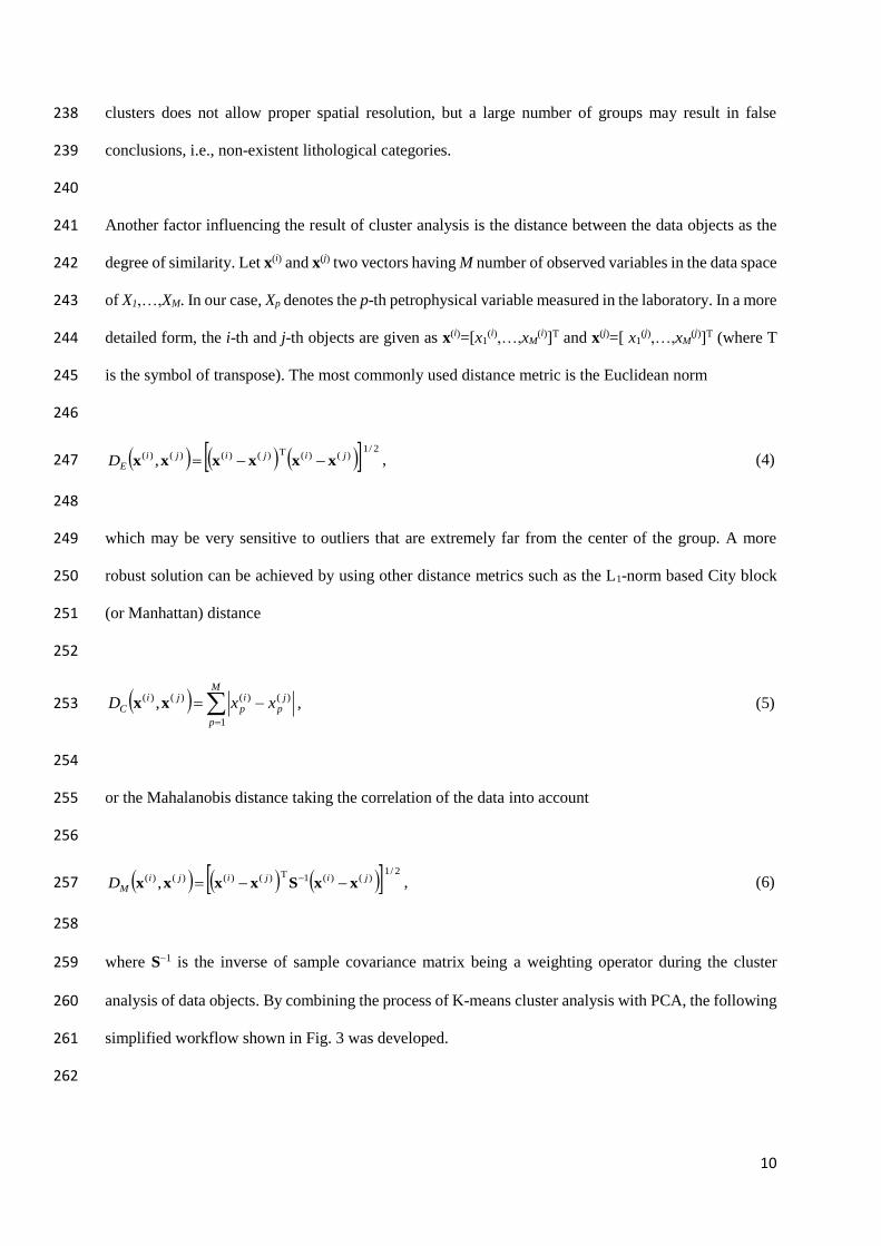
10

clusters does not allow proper spatial resolution, but a large number of groups may result in false 238

conclusions, i.e., non-existent lithological categories. 239

240

Another factor influencing the result of cluster analysis is the distance between the data objects as the 241

degree of similarity. Let x(i) and x(j) two vectors having M number of observed variables in the data space 242

of X1,…,XM. In our case, Xp denotes the p-th petrophysical variable measured in the laboratory. In a more 243

detailed form, the i-th and j-th objects are given as x(i)=[x1(i),…,xM

(i)]T and x(j)=[ x1(j),…,xM

(j)]T (where T 244

is the symbol of transpose). The most commonly used distance metric is the Euclidean norm 245

246

2/1)()(T)()()()( , jijiji

ED xxxxxx , (4) 247

248

which may be very sensitive to outliers that are extremely far from the center of the group. A more 249

robust solution can be achieved by using other distance metrics such as the L1-norm based City block 250

(or Manhattan) distance 251

252

M

p

jp

ip

jiC xxD

1

)()()()( ,xx , (5) 253

254

or the Mahalanobis distance taking the correlation of the data into account 255

256

2/1)()(1T)()()()( , jijiji

MD xxSxxxx , (6) 257

258

where S1 is the inverse of sample covariance matrix being a weighting operator during the cluster 259

analysis of data objects. By combining the process of K-means cluster analysis with PCA, the following 260

simplified workflow shown in Fig. 3 was developed. 261

262

11

263

Fig. 3. Flowchart of the correlation-based interpolation- and principal component analysis assisted 264 clustering method 265

266 In applying the method, we have considered a column as unusable, when it contains only the same 267

values. One can drop these kind of columns without information loss. It must be also mentioned that 268

clustering can be applied with or without dimension reduction. We prefer the use of PCA method in 269

most cases, because it makes possible to highlight the most important features. Unfortunately, it does 270

not provide the meaning of the resulted new dimensions. However, the physical relations between the 271

PCs and petrophysical characteristics may be explored by partial correlation analysis, which can be 272

added as a new element to the workflow. 273

274

3. Case study 275

276

The core samples examined in this study originate from the southern part of the Pannonian Basin 277

Province of Central Europe, where several petroleum systems have been discovered. The Pannonian 278

Basin consists of a large extensional basin of Neogene age overlying Paleogene basins and a Mesozoic 279

(or older) basement (Dolton, 2006). A several kilometers thick large-extension Tertiary basin-fill 280

sedimentary sequence contains oil and gas-bearing formations. The main lithological categories are 281

conglomerate, breccia, calcareous marl, clay, aleurolit, and gravellous sandstone of different grain sizes, 282

dolomite and some basalt. The rock specimen was collected in 28 neighboring wells from an interval of 283

12

1352 m. The full dataset as input for cluster analysis includes 421 core samples and 59 measured 284

petrophysical properties, i.e. carbonate content, bulk and grain density, helium porosity, Klinkenberg-285

corrected permeability, oil and water permeability, irreducible water saturation, sample porosity and 286

volume, mercury saturation in the pressure range of 0.14,000 bar (and pore-throat radii between 287

1.8810375 μm), and water saturation determined by centrifuge method in the pressure range of 0.16 288

and 6 bar. Most of the observed variables were measured both perpendicular and parallel to the axis of 289

the core drilling forming two separate input parameters from the same petrophysical quantity. For the 290

mercury injection and capillary pressure curves, one column of the data matrix contains those saturation 291

values, which were measured on different core samples under the same pressure. The strength of 292

correlation between the observed variables is found to be moderate. We introduce the following scalar 293

called mean spread for the measure of average correlation: 294

2/1

1 1

2

1

1

M

i

M

j

ijij δRMM

S D , (7) 295

where R(D) is the Pearson’s correlation matrix of the observed variables, M is the number of 296

measurement variables and δ is the Kronecker delta function. In this case study, S resulted around 0.6 297

for the data matrix of core measurements. The linear regression connection between some of the studied 298

petrophysical quantities is shown in Fig. 4, where the independent and dependent variables were denoted 299

by x and y, respectively. 300

301

13

302

Fig. 4. Linear relationships between the petrophysical parameters in a Hungarian Miocene complex 303 including the regression equations of porosity vs. bulk density (a), porosity measured perpendicular 304

and parallel to the axis of the core drilling (b), Klinkenberg-corrected permeability vs. porosity (c) and 305 water saturation measured by mercury injection and centrifugal methods (d) 306

307

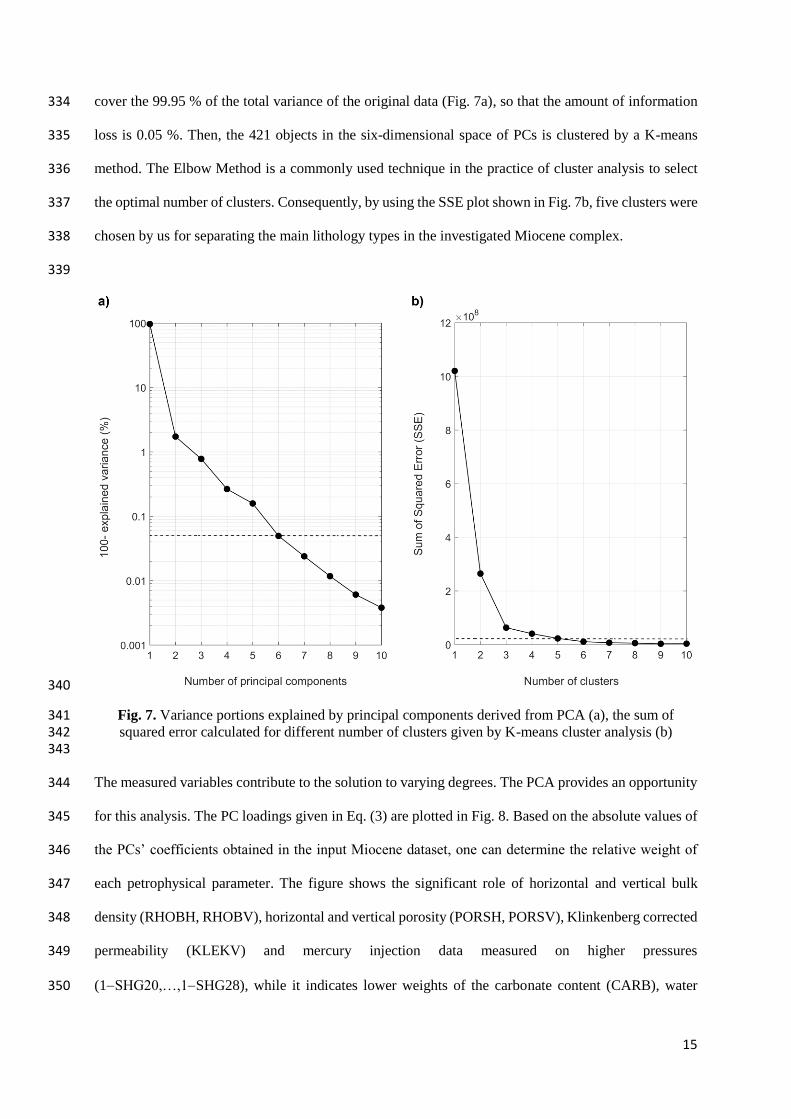
Core data referring to different wells and depth intervals are placed in the data matrix in random order. 308

By using the linear regression functions determined between each pair of measured variables, the 309

missing values in the input data matrix is replaced with synthetic data. Our correlation-based imputation 310

method completely fills out the sparse matrix of the observed variables within their physical boundaries. 311

The image of the original data matrix can be seen in Fig. 5a, where the missing data places are indicated 312

by white color and the values of petrophysical parameters are scaled into the range of 0 and 1. The raw 313

data matrix is incomplete at 71 %. One can notice that the data coming from different wells represent 314

distinct groups of observed variables. It is shown in Fig. 5b that how the proposed statistical approach 315

gives an estimate to the missing cells so that creating a complete data matrix of petrophysical quantities. 316

At the end of this process, the large size data matrix is completed at 100 %. The result of interpolation 317

is plotted for four essential petrophysical parameters in Fig. 6, which forms an appropriate input for the 318

subsequent phase of the clustering procedure. 319

320

14

321

Fig. 5. Input data matrix includes missing values of petrophysical parameters in the investigated 322 Hungarian Miocene complex (a) and fully filled data matrix extracted from the raw dataset using the 323

correlation-based imputation method (b) 324 325

326

Fig. 6. Observed data measured on core samples (dots) and interpolation results for petrophysical 327 parameters in a Hungarian Miocene complex (black line): carbonate content (a), irreducible water 328 saturation (b), sample porosity (c), water saturation derived from mercury injection experiment (d) 329

330

The resultant data matrix is decomposed by PCA according to Eq. (1), which concentrates the common 331

observed information in a few variables. By calculating the eigenvalues of the PCs represented in Eq. 332

(2), a decision can be made for the number of extracted variables. For the processed dataset, six PCs 333

15

cover the 99.95 % of the total variance of the original data (Fig. 7a), so that the amount of information 334

loss is 0.05 %. Then, the 421 objects in the six-dimensional space of PCs is clustered by a K-means 335

method. The Elbow Method is a commonly used technique in the practice of cluster analysis to select 336

the optimal number of clusters. Consequently, by using the SSE plot shown in Fig. 7b, five clusters were 337

chosen by us for separating the main lithology types in the investigated Miocene complex. 338

339

340

Fig. 7. Variance portions explained by principal components derived from PCA (a), the sum of 341 squared error calculated for different number of clusters given by K-means cluster analysis (b) 342

343

The measured variables contribute to the solution to varying degrees. The PCA provides an opportunity 344

for this analysis. The PC loadings given in Eq. (3) are plotted in Fig. 8. Based on the absolute values of 345

the PCs’ coefficients obtained in the input Miocene dataset, one can determine the relative weight of 346

each petrophysical parameter. The figure shows the significant role of horizontal and vertical bulk 347

density (RHOBH, RHOBV), horizontal and vertical porosity (PORSH, PORSV), Klinkenberg corrected 348

permeability (KLEKV) and mercury injection data measured on higher pressures 349

(1SHG20,…,1SHG28), while it indicates lower weights of the carbonate content (CARB), water 350

16

saturation (SW1,…,SW6) and mercury injection data at low pressures (1SHG1,...,1SHG17). 351

Maximal impact on the PCs goes to the Klinkenberg corrected permeability and relative permeability to 352

oil and water (KO, KW). In conclusion, PCA emphasizes primarily the pore structure characteristics 353

and the hydraulic conductivity of the given rock types. 354

355

Fig. 8. Coefficients of principal components indicating the relative weights of petrophysical properties 356 on the solution of PCA in the investigated Hungarian Miocene complex 357

358

Clustering is made to separate the row vectors of observed petrophysical parameters into K=5 classes. 359

To prevent the data processing from the harmful effect of outliers, the City block distance in Eq. (5) is 360

used for the K-means cluster analysis. The grouped data objects in the space of the first three eigenvalues 361

(eig1eig3) is given in Fig. 9a, while the same objects are plotted in the coordinate system of three 362

measured quantities (Fig. 9b) such as carbonate volume including calcite and dolomite contents 363

(CARB), porosity obtained by dynamic displacement on full diameter samples (PORDYN) and relative 364

permeability to water (KW). The figures demonstrate that the clusters are well separated (e.g., the high 365

porosity and permeability reservoirs are indicated with dark yellow color) despite the input dataset being 366

compositionally heterogeneous and unevenly distributed in the space. 367

368

17

369

Fig. 9. Result of PCA of the filled data matrix observed in a Hungarian Miocene complex: 370 transformed data in the coordinate system of eigenvectors (a). Result of cluster analysis: clusters vs. 371

petrophysical variables as input parameters (b) 372 373

374

The result of cluster analysis can be seen in Fig. 10, where the section of cluster numbers in the last 375

track shows to which group the rock samples are classified. It is noted that sudden changes in the 376

resultant cluster numbers are also due to the fact that the core data referring to different depth coordinate 377

(and wells) are quasi-randomly selected along the ordinate axis. The hydrocarbon-bearing formations 378

can be clearly separated in the image of cluster numbers. Cluster 5 represented by yellow color is 379

connected to highly porous and permeable zones with small amount of carbonate (e.g., for samples 380

140160). Petrophysical properties measured both with horizontal and vertical direction to the axis of 381

sampling practically shows just a little amount of anisotropy. The capillary pressure curves indicates 382

high amount of movable fluids in these intervals. The other four clusters indicate less permeable zones 383

with higher amount of carbonate. Cluster 1 and 2 show impermeable formations with much amount of 384

carbonate and high irreducible water saturation (e.g., around the near vicinity of sample 175), while 385

cluster 3 and 4 form a transition between permeable and impermeable rocks (e.g., for samples 170). 386

By comparing the result of cluster analysis to that of the lithology description, cluster 3 and 4 can be 387

identified mostly as conglomerate and clay with some amount of dolomite, respectively. Cluster 5 is 388

mainly composed of sandstone, gravel and fractured breccia with good reservoir storage capacity. 389

Cluster 1 and 2 include calcareous and clayey marls. In the brown intervals, dolomites (e.g., around 390

sample no. 200) and in the blue ones, thin layers of fractured basalt conglomerate are also found (e.g., 391

18

in the range of 290300). The clustering procedure allows the classification of capillary pressure curves 392

by separating different groups (Fig. 11), which makes the interpretation more reliable. Although there 393

is some overlap between the clusters of different pore geometries, the reservoirs of the highest movable 394

wetting phase saturation can be clearly distinguished (see them by yellow color). The full curves of 395

capillary pressure data gives more information than conventional porosity and permeability data. In 396

addition to pore-size geometry distribution, it holds important information also on other textural 397

characteristics of the clustered rock types, which can be further investigated in future studies. 398

399

400

Fig. 10. Cluster analysis of laboratory data measured on core samples collected from a Hungarian 401 Miocene complex: interpolated logs of petrophysical parameters as input for clustering (tracks 1-7), 402

estimated distribution of clusters by using Manhattan distance metric as the result (track 8) 403 404

19

405 406

Fig. 11. Results of clustering of mercury injection data measured on core samples collected from the 407 studied Miocene formations 408

409

4. Discussion 410

411

To test the accuracy of estimation results of the proposed clustering method, a synthetic modeling 412

experiment has been accomplished. An exactly known inhomogeneous petrophysical model is assumed 413

to represent a hydrocarbon formation with varying amount of porosity (), water saturation (Sw), sand 414

volume (Vsd), shale content (Vsh) and carbonate volume (Vc) along a borehole. Theoretical open-hole 415

wireline logging data are calculated and simultaneously processed by cluster analysis to examine how 416

accurately the exact model is reconstructed. The performance of cluster analysis can be tested using 417

arbitrarily chosen amount of noise added to the input data and the rate of incompleteness of the data 418

matrix formed from the noisy synthetic well logs. The following simplified probe response functions 419

summarized by Alberty and Hashmy (1984) are used to calculate the wireline logs (the effect of invasion 420

is neglected in this approach) 421

422

ccsdsdshshhwwwb VVVSSΦ 1 , (8) 423

cccsdsdsdshshshb ρGRVρGRVρGRVρGR 1, (9) 424

20

cecsdesdsheshhewwe,we PVPVPVPSPSΦP ,,,,1 , (10) 425

ccsdsdshshhwww ΔtVΔtVΔtVΔtSΔtSΦΔt 1 , (11)426

n

w

w

m

sh

2

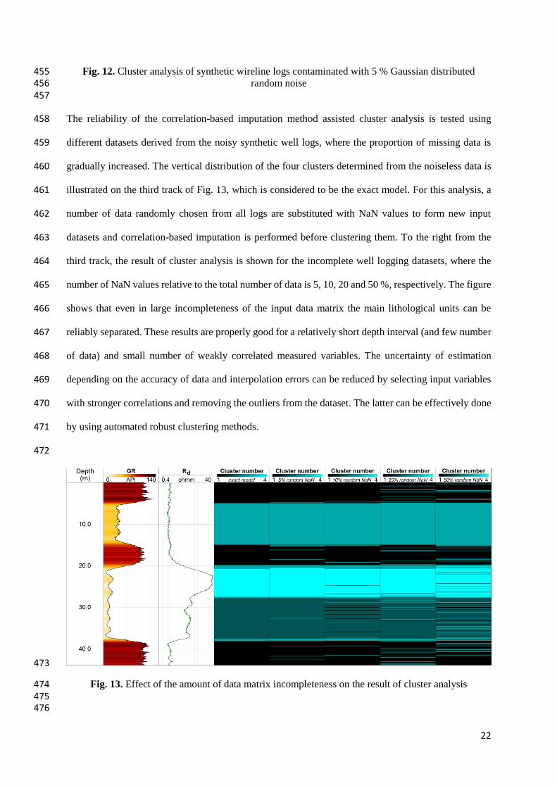
V

sh

d

SaR

Φ

R

V

R

sh

1

1, (12) 427

where the quasi-measured parameters are bulk density (b), natural gamma-ray intensity (GR), 428

photoelectric absorption cross-section index (Pe), acoustic (P-wave) travel-time (t) and deep resistivity 429

(Rd). The functional constants included in Eqs. (8)(12), representing the physical properties of pore 430

fluids, shale and mineral components as well as the textural properties of rocks, are specified in Table 1 431

(we assume gas phase under hydrocarbon). 432

433 Table 1 434 Zone parameters used for calculating synthetic wireline logs to test the accuracy of the proposed cluster 435 analysis method. 436 437

Well log Zone parameter Symbol Selected value Unit

Natural gamma

intensity

(GR)

sand GRsd 10

API shale GRsh 140

carbonate GRc 5

Bulk density

(b)

sand ρsd 2.65

g/cm3

shale ρsh 2.55

carbonate ρc 2.79

pore-water ρw 1.09

hydrocarbon ρh 0.016

Sonic interval-

time

(t)

sand Δtsd 56

µs/ft

shale Δtsh 108

carbonate Δtc 46

pore-water Δtw 200

hydrocarbon Δth 305

Photoelectric

index

(Pe)

sand Pe,sd 1.81

barn/e

shale Pe,sd 3.50

carbonate Pe,sd 4.11

pore-water Pe,sd 0.81

hydrocarbon Pe,sd 0.09

Deep resistivity

(Rd)

shale Rsh 1 m

pore-water Rw 0.06

cementation

exponent m 2.0

saturation exponent n 2.0

tortuosity

coefficient a 1.0

21

In this uncertainty analysis, 5 % Gaussian distributed noise is added to the synthetic data calculated in 438

the forward modeling procedure using Eq. (8)-(12). The mean spread (defined in Eq. (7)) calculated for 439

the noisy well logging parameters is 0.44, which represents weak correlation relationship between the 440

five input variables on the average. The full correlation matrix is given in Table 2. 441

442

Table 2 443 Pearson’s correlation matrix of synthetic well logs including 5 % Gaussian noise. 444 445

GR Pe b t Rd

GR 1 0.54 0.44 0.23 0.50

Pe 0.54 1 0.61 0.38 0.49

b 0.44 0.61 1 0.34 0.50

t 0.23 0.38 0.34 1 0.25

Rd 0.50 0.49 0.50 0.25 1

446

The exactly known petrophysical model can be seen in tracks 12 in Fig. 12, where 6 layers can be 447

distinguished: 5 m thick shale, 10 m thick water-bearing sandstone, 5 m thick shale, 8 m thick 448

hydrocarbon-bearing sandstone, 10 m thick limestone and 6 m thick shale. By assuming 4 main 449

lithological units, the entire well logging dataset (plotted in tracks 3-7) is processed by K-means cluster 450

analysis (in this test PCA is not necessary to be applied). As a result, the depth variation of cluster 451

numbers is shown in the last track. 452

453

454

22

Fig. 12. Cluster analysis of synthetic wireline logs contaminated with 5 % Gaussian distributed 455 random noise 456

457

The reliability of the correlation-based imputation method assisted cluster analysis is tested using 458

different datasets derived from the noisy synthetic well logs, where the proportion of missing data is 459

gradually increased. The vertical distribution of the four clusters determined from the noiseless data is 460

illustrated on the third track of Fig. 13, which is considered to be the exact model. For this analysis, a 461

number of data randomly chosen from all logs are substituted with NaN values to form new input 462

datasets and correlation-based imputation is performed before clustering them. To the right from the 463

third track, the result of cluster analysis is shown for the incomplete well logging datasets, where the 464

number of NaN values relative to the total number of data is 5, 10, 20 and 50 %, respectively. The figure 465

shows that even in large incompleteness of the input data matrix the main lithological units can be 466

reliably separated. These results are properly good for a relatively short depth interval (and few number 467

of data) and small number of weakly correlated measured variables. The uncertainty of estimation 468

depending on the accuracy of data and interpolation errors can be reduced by selecting input variables 469

with stronger correlations and removing the outliers from the dataset. The latter can be effectively done 470

by using automated robust clustering methods. 471

472

473

Fig. 13. Effect of the amount of data matrix incompleteness on the result of cluster analysis 474 475

476

23

The aforementioned synthetic modeling experiment focuses mainly on the effect of the accuracy of 477

original measurements and the interpolation error when replacing the unknown values with estimated 478

ones. Besides these types of noises added to the dataset, the data also include other sources of 479

uncertainty. For a more detailed uncertainty analysis, we have to consider basically three types of errors. 480

At first, one has to quantify the error of the original measurements. The estimation of measurement 481

errors makes it necessary to know the features of the measurement process. Secondly, our model 482

assumes linear connection between all the columns in the data matrix. For a better approximation, one 483

has to consider the underlying physical relations among the columns, which is unknown in most of the 484

cases. At last, the accumulated estimation errors should also be taken into consideration. It is the result 485

of the incremental nature of the imputation algorithm giving an estimate in the actual iteration from the 486

estimated values of earlier iterations. In the ideal case, only the considered value is missing, which 487

means that the estimation is based on the available measurements. In the worst case, all values of the 488

selected columns are estimated. This kind of accumulated estimation error depends on the rate of the 489

counts of measured and predicted values having used for the given estimation. 490

491

5. Conclusions 492

493

In the paper, an improved clustering algorithm is proposed for the interpretation of core datasets 494

originating from heterogeneous sources. A correlation-based multi-linear regression method is first used 495

for the filling of typically incomplete data matrices, which gives a suitable input for the K-means cluster 496

analysis performed in a subsequent data processing step. After the upload phase, all variables are taken 497

into account during the clustering, but it is also possible to select the parameters individually based on 498

the results of principal component analysis. Those parameters with relative small PC coefficients can be 499

neglected. Since there is no limit for the approach on the number of processed variables forming the 500

input dataset, the clustering method is suitable for the future expansion of observed parameters. Based 501

on this, not only new petrophysical parameters, but also mineralogical (e.g., from X-ray diffraction) and 502

other compositional (e.g., geochemistry) data may be involved. An added advantage of the statistical 503

method is the grouping possibility of the capillary pressure curves, which helps to integrate more 504

24

information on the textural and fluid characteristics of the investigated formations. (The analysis of these 505

curves has wide literature, which is beyond the scope of this paper.) The explanation of the behavior of 506

these curves are typically given on an empirical basis in the literature. However, an analytic description 507

may reveal new petrophysical characteristics of the studied formations. In addition to the measured 508

parameters of such analytic models, for a more reliable interpretation of the pore structure (textural 509

properties), pore-fluid types (bound or free water and hydrocarbons) and properties (e.g., viscosity), T2 510

relaxation time distribution curves of nuclear magnetic resonance measurements can also be added as 511

input in future applications. 512

513

Cluster analysis is commonly used also for the processing of wireline logging data. Well log derived 514

petrophysical parameters such as porosity, shale volume, matrix volumes, water and hydrocarbon 515

saturation, permeability etc. as high resolution in situ information can significantly increase the size of 516

the statistical sample and may further improve the performance of cluster analysis. The big amount of 517

data is processed by linear regression and classical K-means clustering algorithm for a quick 518

interpretation. For obtaining a more reliable solution, a robustified cluster analysis approach including 519

a nonlinear interpolation method as imputation phase can be used in the future. As a statistically highly 520

efficient method, the most frequent value-based (automated) weighting procedure introduced by Steiner 521

(1991) gives a robust solution independent from the nature and statistical distribution of the input dataset 522

(e.g., in Zhang, 2017). As a first result, its application to clustering of well logs can be found in Braun 523

et al. (2016), which will be followed by improved clustering algorithms in the near future as intensive 524

research is currently made at the Department of Geophysics, University of Miskolc. The resultant 525

clusters can also be easily correlated between the wells to represent the spatial distribution of clusters 526

for two- and three-dimensional cases. 527

528

Acknowledgments 529

530

The authors would like to thank the experts and staff at the MOL group for their valuable cooperation 531

and for the measurement and laboratory data they provided. This research was supported by the 532

25

European Union and the Hungarian State, co-financed by the European Regional Development Fund in 533

the framework of the GINOP-2.3.4-15-2016-00004 project, aimed to promote the cooperation between 534

the higher education and the industry. 535

536

References 537

538

Alberty, M., and K. Hashmy, 1984. Application of ULTRA to log analysis: Presented at the SPWLA 539

Symposium Transactions, 1–17. 540

Braun B. A., Abordán A., Szabó N. P., 2016. Lithology determination in a coal exploration drillhole 541

using Steiner weighted cluster analysis. Geosciences and Engineering 5 (8), 51–64. 542

Candès E. J., Recht B., 2009. Exact matrix completion via convex optimization. Foundations of 543

Computational mathematics 9(6), 717–772. 544

Cranganu C., Luchian H., Breaban M. E., 2015. Artificial intelligent approaches in petroleum 545

geosciences. Springer. 546

Dolton G. L., 2006. Pannonian Basin Province, Central Europe (Province 4808) – Petroleum geology, 547

total petroleum systems, and petroleum resource assessment, USGS Bull. 2204–B, 1–47. 548

Gemulla R., Nijkamp E., Haas P. J., Sismanis Y., 2011. Large-scale matrix factorization with distributed 549

stochastic gradient descent. In Proceedings of the 17th ACM SIGKDD international conference on 550

Knowledge discovery and data mining, ACM, 69–77. 551

Hartigan J. A., Wong M. A., 1979. Algorithm AS 136: A k-means clustering algorithm. Journal of the 552

Royal Statistical Society. Series C (Applied Statistics), 28.1, 100–108. 553

Hempkins W. B., 1978. Multivariate statistical analysis in formation evaluation. SPE California 554

Regional Meeting, San Francisco, 7144–MS. 555

26

Jarzyna J. A., Bała M., Krakowska P. I., Puskarczyk E., Strzępowicz A., Wawrzyniak-Guz K., Więcław 556

D., Ziętek J., 2017. Shale Gas in Poland, Advances in Natural Gas Emerging Technologies. IntechOpen, 557

DOI: 10.5772/67301. 558

Jolliffe I.T., 2002. Principal component analysis, 2nd edition, New York, Springer-Verlag. 559

Jung H., Jo H., Kim S., Lee K., Choe J., 2018. Geological model sampling using PCA-assisted support 560

vector machine for reliable channel reservoir characterization. Journal of Petroleum Science and 561

Engineering 167, 396405. 562

Lawley D. N., Maxwell A. E., 1962. Factor analysis as a statistical method. The Statistician 12, 209–563

229. 564

Little R., Rubin B., 1986. Statistical Analysis with Missing Data, John Wiley & Sons, Inc., New York. 565

Ma Z., Holditch S., 2015. Unconventional Oil and Gas Resources Handbook: Evaluation and 566

Development. Gulf Professional Publishing. 567

Masoudi P., Aïfa T., Memarian H., Tokhmechi B., 2018. Uncertainty assessment of porosity and 568

permeability by clustering algorithm and fuzzy arithmetic. Journal of Petroleum Science and 569

Engineering 161, 275290. 570

Mazumder R., Hastie T., Tibshirani R., 2010. Spectral regularization algorithms for learning large 571

incomplete matrices. Journal of Machine Learning Research 11, 2287–2322. 572

Skalinski M., Gottlib-Zeh S., Moss B., 2006. Defining and predicting rock types in carbonates – 573

Preliminary results from an integrated approach using core and log data from the Tengiz Field. 574

Petrophysics 47 (1), 37–52. 575

Steiner F., 1991. The most frequent value: Introduction to a modern conception of statistics. Akadémiai 576

Kiadó, Budapest. 577

27

Szabó N. P., Dobróka M., Kavanda R., 2013. Cluster analysis assisted float-encoded genetic algorithm 578

for a more automated characterization of hydrocarbon reservoirs. Intelligent Control and Automation 4 579

(4), 362–370. 580

Szabó N. P., Dobróka M., 2017. Robust estimation of reservoir shaliness by iteratively reweighted factor 581

analysis. Geophysics 82 (2), D69–D83. 582

Szabó N. P., Dobróka M., 2018. Exploratory factor analysis of wireline logs using a Float-Encoded 583

Genetic Algorithm. Mathematical Geosciences 50 (3), 317–335. 584

Zhang J., 2017. Most frequent value statistics and distribution of 7Li abundance observations. Monthly 585

Notices of the Royal Astronomical Society 468 (4), 5014–5019. 586

587

Appendix 588

589

A simplified pseudo-code of the imputation algorithm applied in the proposed workflow, where m 590

denotes the total number of columns of the input data matrix (i.e., measured petrophysical parameters, 591

here variables x and y) and n is the total number of rows of the same matrix (i.e., core samples). 592

593

for i := 1 to m - 1 594

for j := i + 1 to m 595

x := i-th column of the data matrix 596

y := j-th column of the data matrix 597

points = {(xk, yk) : xk != NaN, yk != NaN, 1 <= k <= n} 598

fit linear model to points by linear regression 599

for k := 1 to n 600

if xk != NaN and yk == NaN 601

yk := fitted value by the linear model from xk 602

end 603

if xk == NaN and yk != NaN 604

xk := fitted value by the linear model from yk 605

end 606

28

end 607

end 608

end 609