Cluster Randomised Controlled Trials

STATS 773: DESIGN AND ANALYSIS OF CLINICAL TRIALS

Dr Yannan Jiang

Department of Statistics

May 14th 2012, Monday, 09:00-10:30

Cluster Randomised Trial

Hospitals (2N)

A group of individuals is randomly allocated to receive either the intervention or the control

Intervention (N)

Control (N)

Randomisation (1:1) Follow-up of patients

2

Cluster Randomised Trials (CRT)

• Unit of randomisation is a cluster (i.e. a group of individual subjects)

- GP clinic, hospital, school, geographic area

• Data collection is often at the individual level - Blood pressure, BMI

- Number of hospital admissions

- Time to healing

• Subjects in the same cluster are more like one another than those in different clusters

- Patients registered at the same clinic - Students who attend the same school

3

Why do CRT?

• Intervention at the level of a cluster – All individuals in the same cluster will receive the

same intervention

– Administrative convenience , e.g. new hypertension screening implemented at a GP clinic

• Possibility of contamination – Individuals in the same cluster may influence each

other and dilute the treatment effect

• Potential ethical issues – Seems unethical to treat patients in the same clinic

differently

4

Complexity with CRT • Randomisation is limited by the number of clusters

recruited to the study – Often small due to logistic and budget – Clusters may vary, and hard to match or stratify

• Reduced effective sample size than individual randomized trials – Correlation among individuals in the same cluster need to be taken

into account – The design effect is related to Intra-cluster Correlation Coefficient

(ICC) and the number of individuals per cluster (m)

• Methods ignoring clustering may mislead data analysis – Assume independence among correlated observations within the

same cluster – Standard errors and confidence intervals tend to be too small – Small P-values introduce false positive results

5

A Simulation Study

• Two groups, with two clusters per group and 10 subjects per cluster

• Generate four cluster means 𝑌𝑗 and a random sample within each cluster – 𝑌𝑗 ~ Normal (mean=10, SD=2)

– 𝑌𝑖𝑗~ Normal (mean=0, SD=1)

• TRUE null hypothesis: No difference between the means in the two groups

• Conduct simple two-sample t-test using: – Individual sample data (𝑌𝑖𝑗) ignoring the clustering

– Four group means (𝑌𝑗 ) only

Workshop: Cluster Randomised Trials, Prof Martin Bland 6

1000 Simulation Results

• What we expect to see: – With a valid test, we expect

• 50 (5%) significant differences with p-value < 0.05

• 10 (1%) significant differences with p-value < 0.01

• What we actually see in simulations: – With a two-sample t-test using individual data ignoring the

clustering • 600 (60%) significant differences with p-value < 0.05

• 502 (50.2%) significant differences with p-value < 0.01

– With a two-sample t-test using four cluster means only • 53 (5.3%) significant differences with p-value < 0.05

• 14 (1.4%) significant differences with p-value < 0.01

Workshop: Cluster Randomised Trials, Prof Martin Bland 7

Intra-cluster Correlation Coefficient (ICC)

• A measure of the relatedness of clustered data by comparing the variance within clusters with the variance between clusters

• Two sources of variability with clustered data: – Variance within the cluster (𝜎𝑤

2)

– Variance between the clusters (𝜎𝑏2)

• ICC is calculated as:

• ICC ranges from 0 to 1

– ρ=0 indicates no correlation between subjects within a cluster, i.e. same as a simple random sample

– ρ=1 indicates all subjects within a cluster are identical, i.e. m=1 (the worse case scenario)

8

Estimation of ICC (1)

• We can estimate ICC from the analysis of variance (ANOVA) table with a continuous outcome

One-way Analysis of Variance:

Source Sum of Squares DF Mean Square F-test

Between classes BSS BDF=g-1 BMS=BSS/BDF BMS/WMS

Within class WSS WDF=g(m-1) WMS=WSS/WDF

Total BSS+WSS BDF+WDF

ICC = (BMS – WMS) / [BMS + (m-1)WMS], or equivalently,

ICC = (F – 1) / (F + m – 1)

Here g is the number of classes, m the number of subjects per class

9

Estimation of ICC (2)

• For binomial responses, e.g. the success rate, an analogous measure to ICC is the kappa coefficient (κ) – Only work for small clusters (e.g. m=2)

• Let p* the proportion of the control group with concordant clusters – A concordant cluster with κ=1 is the one where all

responses within a cluster are identical

• Let pc the underlying success rate in the control group

• The kappa coefficient is estimated as: {p* - [pc

m + (1-pc)m]} / {1 - [ pc

m + (1-pc)m ]}

10

Sources of ICC

• The following sources may be used to estimate the ICC for a new trial:

– Pilot study data

– Other trials with similar clusters and outcome variable

• Many trial reports do not give the ICC!

11

Design Effect and Sample Size

• The design effect for a CRT with equal sized cluster is: Deff = 1 + (m - 1) * ICC

– m is the number of subjects per cluster – ICC is the intra-class correlation coefficient

• The required sample size for a CRT is estimated as:

Nc = Ns * Deff,

– Nc is the sample size for a cluster randomised trial – Ns is the sample size for a standard randomised controlled trial – Same when Deff=1 (i.e. m=1 or ICC=0)

• With unequal sized cluster, m is replaced by 𝑚 where

12

Size of Clusters

• Unequal cluster sizes increase the design effect

13

Workshop: Cluster Randomised Trials, Prof Martin Bland

Number of Clusters

• The design effect depends on variances both within and between the clusters

• With small number of clusters per group, 𝜎𝑏2 has few

degrees of freedom and the t-distribution needs to be used rather than the Normal

• In large sample approximation, sample size calculation has the multiplier , where 𝑍𝛽 is now

replaced by t-statistics with a small df

– This will reduce the effective sample size even more!

2

2/ )( zz

14

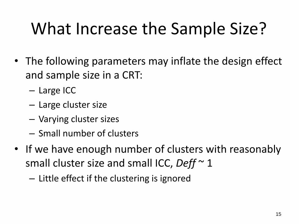
What Increase the Sample Size?

• The following parameters may inflate the design effect and sample size in a CRT:

– Large ICC

– Large cluster size

– Varying cluster sizes

– Small number of clusters

• If we have enough number of clusters with reasonably small cluster size and small ICC, Deff ~ 1

– Little effect if the clustering is ignored

15

Statistical Analysis

• A method that accounts for the cluster effect will be valid and efficient, compared to the naïve method ignoring correlated observations within a cluster

• Several analysis approaches can be used: – Simple analysis adjusting for SEs with the design effect

– Summary statistics at the cluster-level

– Robust variance estimates

– Multilevel models

– Generalized estimating equations (GEE)

– Others, e.g. Bayesian hierarchical models

16

Simple Adjustment of Standard Tests

• Carry out standard tests on individual data assuming there is no clustering

• Adjust the standard error (SE) by multiplying with the square root of the design effect

• Calculate the associated p-value and confidence interval using the adjusted SE

No longer recommended with other advanced methods widely available…

17

Simple Adjustment of Standard Tests

Advantages

• Simple

• Quick

Disadvantages

• Crude adjustment

• No adjustment for covariates

• Only valid when clusters are of equal size

18

Cluster-Level Analysis • A two-stage process

1. A summary measure of study endpoint is obtained for each cluster, with ci estimates per group

2. Statistical inference is made on cluster-level summaries

• Point estimates are obtained for each group using – cluster summaries

– individual values to account for unequal cluster sizes

– log transformation to account for skewed distribution of summary data

• Statistical inferences – Parametric T-test

• Reasonably robust to departure from the underlying assumptions

– Nonparametric Cluster Permutation test • An exact test permuting the treatment assignment to estimate the distribution

of the test statistics under the null hypothesis of no treatment effect • Use clusters of observations rather than individual observations • Make no distributional assumptions

19

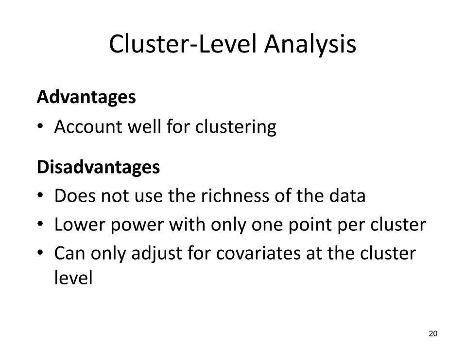
Cluster-Level Analysis

Advantages

• Account well for clustering

Disadvantages

• Does not use the richness of the data

• Lower power with only one point per cluster

• Can only adjust for covariates at the cluster level

20

Robust Standard Error Estimate

• Huber-White standard errors are used to allow the fitting of a model that contains heteroscedastic residuals in a clustered sampling

• The sandwich estimator yields asymptotically consistent and robust covariance matrix estimates

– without making distributional assumptions

– valid even if the assumed model is incorrect

• Can be implemented using SPSS, STATA, SAS

21

Huber-White Robust Estimate

Advantages

• Take into account ICC in data analysis

• Can adjust for individual-level covariates

Disadvantages

• Does not work well if the number of clusters is small, i.e. < 10 clusters

– Normally requires 30 or more clusters

22

Multilevel Models

• Special form of mixed model regression where the data has a hierarchical structure – Cluster and individual levels – Can handle more than two levels, e.g. repeated observations

on each individual

Advantages: – Allows complex correlation structure and additional clustering – Adjust for both cluster and individual level covariates

Disadvantages: – Computationally intensive, and may have convergence

problem – Does not work well with small number of clusters

23

Fixed and Random Effects

• Fixed effect – A factor is regarded as a fixed effect if the categories

that were studied are the only relevant categories

– This is unlikely

• Random effect – The categories that were actually studied represent

only a sample of those potentially available for study from the population of interest

– More plausible

24

A Simple Mixed Model

• Fixed effects model: Outcome = Mean + Treat + Cluster + error – The cluster effect is estimated for each

cluster (df = g - 1) – Random error only

• Random effects model: Outcome = Mean + Treat + Cluster + error

– The cluster variable has 0 mean and unknown variance (df = 1)

– Random cluster effect plus error

25

A Simple Mixed Model

• Model assumptions – Both random cluster effect and random error have Normal

distributions with mean zero and uniform variances

– Independent fixed and random effects

– Uniform correlations between pairs of subjects in a cluster

• Model fit – Iteratively using Restricted Maximum Likelihood (REML)

and the Expectation Maximization (EM) algorithm

– ICC can be directly estimated from the cluster (𝜎𝑏2) and

residual (𝜎𝑤2) variances

26

Generalized Estimating Equations (GEE)

Steps in fitting a GEE model: 1. Choose an appropriate correlation structure for the clustered

data

2. Fit a standard regression model

3. Specify a working correlation matrix

4. Estimate the residuals from regression model

5. Use the empirical distribution of residuals to estimate the correlation parameters

6. Refit model using a modified algorithm incorporating correlation matrix estimated in Step 5

7. Re-estimate the residuals

8. Repeat steps 4-7 until the estimate is converged

27

Working Correlation Structure

23

2

2

32

643

652

451

321

Independent

Exchangeable

00

00

00

t1 t2 t3

t1

t2

t3

Autoregressive

Unstructured

28

GEE Models

Advantages • Do not require a Normal distribution • Provides robust standard error even if correlation

structure is incorrectly specified • Allow for both cluster and individual level covariates

Disadvantages • Treat cluster effect as a nuisance parameter (only if

interested) • Do not extend easily to more than two levels • Standard errors can be unreliable with small number

of clusters

29

Subject-Specific vs Population-Averaged

• Subject-specific approach

– The random effects are modelled

– Estimates the change in expected response for an individual cluster

– Appropriate when prediction is required for the cluster

• Population-averaged approach

– Fixed effects are modelled

– Estimates the expected response for the overall population of clusters

30

GEE and Multilevel Models

31

• GEE fits marginal models – The treatment effect is estimated as the population average from

which the sample is chosen

• Multilevel models are subject-specific – It estimates the treatment effect given a subject’s values of the

other covariates

• GEE estimates are – More sensitive to missing data

– Generally smaller for non-Normal data

• Both are more efficient than cluster-level approaches with – Large numbers of clusters

– Both cluster and individual level covariates

– Hieratical data structure

Stepped-Wedge Design in CRT

• Stepped-wedge cluster randomised trial (SWCRT) involves sequential roll-out of an intervention to clusters of individuals over a number of time periods

• The order in which a proportion of clusters switch from control to intervention is determined randomly by sequences

• All clusters receive the intervention eventually and ideally stay on

• Individual level data are collected repeatedly at each time period

32

The Design Matrix

T1 T2 T3 T4

Sequence 1

Sequence 2

Sequence 3

Sequence 4

Study start Study end

Note: Shaded cells represent intervention periods; Blank cells represent control periods

Study periodBefore After

Study period After

T1

Sequence 1

Sequence 2

Sequence 3

Sequence 4

Study end

Before

Study start

Standard CRT (sequence doesn’t matter)

SWCRT

33

Population-Based Interventions

• General population of interest – Multi-centre trial across a number of cities, provinces,

countries, etc.

– Logistically impossible to implement the intervention simultaneously.

– Practical and financial constraints

• Policy and ethical considerations – Intervention is likely to do more good than harm, but

require population-based evidence

– Unethical to withhold or withdraw intervention from participants

– Roll out the intervention during and after the study

34

The Gambia Hepatitis Intervention Study*

• A large-scale vaccination project to introduce the national hepatitis B (HBV) vaccination to young infants progressively over a 4-year period, initial in July 1986.

• Rationale for the study summarised in the report of WHO meeting on the prevention of liver cancer:

"... it was recognized that it would be undesirable to consider immunization on a widespread scale without, at the same time, organizing studies that were designed to establish whether or not the vaccine was producing a reduction in the incidence of the carrier state and subsequently cancer ... The best method of ensuring that a protective effect of immunization could be measured would be to use randomized controlled trials ... Such a randomized trial would present ethical problems if sufficient vaccine were available to treat all newborn children. At present, and probably for the next several years, however, this is not the position as the vaccine is expensive and supplies are limited."

* The Gambia Hepatitis study group, Cancer Research, 47:5782-87, 1987

35

The Gambia Hepatitis Intervention Study

Points to consider in the design of an appropriate RCT:

– Expense of the vaccine and its limited availability prohibiting immediate universal HBV vaccination

– Desirability of having comparison groups available from same time period

– Severe logistic and ethical difficulties with randomisation at individual level (team/field conditions, multiple doses p.p., infants at the same clinic treated differently, etc.)

– At the end of the study, the HBV vaccine should be widely available with a nationwide delivery system in place

These considerations lead to a “Stepped Wedge” design!

36

17 define country areas

17 teams to initiate

intervention in a

random order

3 months per step

4 years in total

37

The Gambia Hepatitis Intervention Study

Differences in SW Design

• Intervention is delivered in a stepped-wedge fashion where a rigorous evaluation of the effectiveness of intervention is desirable

– Clusters act as their own control, with repeated individual data collected from both control and intervention “wedge”

– Evaluation of the intervention effect is conducted by comparing the data between the control and intervention wedges

• All participants will receive the intervention in a random order, during and potentially after the trial period

– Different from parallel and cross-over designs

38

Different Study Designs

39

1 = intervention phase; 0 = control phase

Sample size in SWCRT

• More complicated and different from standard CRT

Basic parameters in CRT:

– Study power (1-β) and significance level (α)

– Size of expected treatment effect (ε)

– ICC, or similarly the Coefficient of Variation (CV)

• Ratio of between-cluster standard deviation over the mean prevalence

– Number of clusters

– Number of individuals per cluster

Other parameters:

– Number of sequences (steps) and time periods (T) in the wedge

– Number of control (0) and intervention (1) phases in the design

40

Design of SWCRT

• Randomisation – One or more clusters will be randomly allocated to each

sequence of treatment • E.g. 40 hospitals (clusters) with 4 groups of 10s were randomly

allocated to 4 sequences (steps)

• Data collection – All participants in each of the clusters will ideally provide

individual level data repeatedly at the end of each time period • E.g. clinical data on all patients in 40 hospitals will be collected at

scheduled visits when the intervention rolls out sequentially

41

Analysis of SWCRT

• Random effects are commonly used to model the correlation between individuals within the same cluster

• Statistical modelling appropriate for SWCRT design needs to take into account: – Cluster effect (individuals more correlated within a cluster)

– Repeated measures on the same individual

– Secular (time) trend

• The following analysis approaches can be used: – Multilevel models

• Linear Mixed models (LMM)

• Generalized Linear Mixed models (GLMM)

– Generalised estimating equations (GEE)

42

The Statistical Model

For a design with I clusters, T time points, and N individuals sampled per cluster per time interval.

Let Yijk be the outcome of individual k at time j from cluster i, and Yij be the mean of cluster i at time j.

Define , where

• αi is a random effect for cluster i, with

• βj is a fixed effect at time j

• Xij is an indicator of treatment phase (1 vs 0 ) in cluster i at time j

• θ is the treatment effect

43

Design and analysis of stepped wedge cluster randomized trials, Hussey and Hughes (2007)

The Statistical Model

• A model for individual level outcome is:

• A model for the cluster means is:

44

Design and analysis of stepped wedge cluster randomized trials, Hussey and Hughes (2007)

Power Calculation

• Provide statistical justification of the study power for a selected sample size

• We want to test the following hypothesis:

HO: θ=0 versus HA: θ=θA

• The approximate power for a two-sided test at α level of significance is given as:

- where φ is cumulative standard Normal distribution function

45

Power Calculation

• Assuming equal N per cluster per time interval,

• For a binary outcome where the cluster level response is a proportion, it is reasonable to assume that

46

A Case Study – BISkIT Trial

• A SWCRT to determine whether provision of a free school breakfast improves attendance, academic performance, nutrition and food security in children attending primary schools in deprived areas in New Zealand

– 14 schools in low socioeconomic resource areas were randomised

– 424 Year1 - 8 school students participated in the study

– Primary outcome: Children’s school attendance, measured as

• Achievement of a school attendance rate of 95% or higher in a term

• School attendance rate (%)

– Secondary outcomes: academic achievement, self-reported grades, sense of belonging at school, short-term hunger, food security

47

Recruit

Schools

Randomise

schools

Recruit

students

Intervention Control Control Control

Intervention Intervention Control Control

Intervention Intervention Intervention Control

Intervention Intervention Intervention Intervention

Term 1

Demographics

& Assess

Term 2

Assess

Term 3

Assess

Term 4

Assess

Four sequences

Process evaluation

48

Study Design and Analysis

• The target sample size was 16 schools (4 schools per sequence) with on average 25 students per school, a total of 400 participants followed over 4 terms in a school year

• Assuming an intra-cluster coefficient (ICC) of 0.05, this sample size would provide at least 85% power at 5% level of significance to detect a 10% absolute increase in the proportion of children with an attendance rate of 95% or higher

• Generalized Linear Mixed Model (GLMM) was used to evaluate the main treatment effect between intervention and control phases, controlling for individual covariates and the school term

49

SAS Example Code

PROC GLIMMIX;

CLASS Cluster ID Treatment Time;

MODEL Y1 = X1 Treatment Time / SOLUTION DDFM=satterth

ODDSRATIO DIST=binary LINK=logit;

RANDOM Cluster;

RANDOM _residual_ / SUBJECT=ID TYPE=CS;

RUN;

PROC MIXED;

CLASS Cluster ID Treatment Time;

MODEL Y2 = X2 Treatment Time / SOLUTION DDFM=satterth;

RANDOM Cluster;

REPEATED Time / SUBJECT=ID TYPE=UN;

RUN;

50

Systematic Review of SWCRT (1)

51

Brown and Lilford (2006)

52

Systematic Review of SWCRT (2)

53

Mdege et al. (2011)

Compared with the first SR,

– Expanded search to non-health care trials

– Focus on randomised studies and cluster allocations

– Aim to describe the application of SWCRT design in evaluating the effectiveness of interventions

• Areas of research involved

• Motivation for using the design

• General characteristics of the design

• Method of data analysis

• Quality of reporting

54

Note: Heading and subheadings adapted from the CONSORT statement for reporting cluster randomised trials.

55

An MSc Student Project

56 Lennex Yu (2011)

14 New Studies Identified

57

Overall Summary

• An increasing number of SWCRT have been reported in recent years

• More studies are published from the developed than developing countries

• The methodological reporting is still sub-optimal in some studies and may lack appropriate information on sample size calculation, randomization method, data collection and analysis

58

Published Studies by Year and Country

0

1

2

3

4

5

6

80s 90s 2002 2003 2004 2005 2006 2007 2008 2009 2010 2011

Nu

mb

er

of

Pu

blic

atio

n

Year

Developing Countries Developed Countries

59

A World Map of Published Studies by Trial Location

60