Embed Size (px)
Citation preview
Computer Science and Data Analysis Series
Boca Raton London New York Singapore
Boris Mirkin
Clustering forData Mining
A Data Recovery Approach
Published in 2005 byChapman & Hall/CRC Taylor & Francis Group 6000 Broken Sound Parkway NW, Suite 300Boca Raton, FL 33487-2742
© 2005 by Taylor & Francis Group, LLCChapman & Hall/CRC is an imprint of Taylor & Francis Group
No claim to original U.S. Government worksPrinted in the United States of America on acid-free paper10 9 8 7 6 5 4 3 2 1
International Standard Book Number-10: 1-58488-534-3 (Hardcover) International Standard Book Number-13: 978-1-58488-534-4 (Hardcover) Library of Congress Card Number 2005041421
This book contains information obtained from authentic and highly regarded sources. Reprinted material isquoted with permission, and sources are indicated. A wide variety of references are listed. Reasonable effortshave been made to publish reliable data and information, but the author and the publisher cannot assumeresponsibility for the validity of all materials or for the consequences of their use.
No part of this book may be reprinted, reproduced, transmitted, or utilized in any form by any electronic,mechanical, or other means, now known or hereafter invented, including photocopying, microfilming, andrecording, or in any information storage or retrieval system, without written permission from the publishers.
For permission to photocopy or use material electronically from this work, please access www.copyright.com(http://www.copyright.com/) or contact the Copyright Clearance Center, Inc. (CCC) 222 Rosewood Drive,Danvers, MA 01923, 978-750-8400. CCC is a not-for-profit organization that provides licenses and registrationfor a variety of users. For organizations that have been granted a photocopy license by the CCC, a separatesystem of payment has been arranged.
Trademark Notice:
Product or corporate names may be trademarks or registered trademarks, and are used onlyfor identification and explanation without intent to infringe.
Library of Congress Cataloging-in-Publication Data
Mirkin, B. G. (Boris Grigorévich)Clustering for data mining : a data recovery approach / Boris Mirkin.
p. cm. -- (Computer science and data analysis series ; 3)Includes bibliographical references and index.ISBN 1-58488-534-3 1. Data mining. 2. Cluster analysis. I. Title. II. Series.
QA76.9.D343M57 2005
006.3'12--dc22 2005041421
Visit the Taylor & Francis Web site at http://www.taylorandfrancis.com
and the CRC Press Web site at http://www.crcpress.com
Taylor & Francis Group is the Academic Division of T&F Informa plc.
C5343_Discl Page 1 Thursday, March 24, 2005 8:38 AM
Chapman & Hall/CRC
Computer Science and Data Analysis Series
The interface between the computer and statistical sciences is increasing,as each discipline seeks to harness the power and resources of the other.This series aims to foster the integration between the computer sciencesand statistical, numerical, and probabilistic methods by publishing a broadrange of reference works, textbooks, and handbooks.
SERIES EDITORSJohn Lafferty, Carnegie Mellon UniversityDavid Madigan, Rutgers UniversityFionn Murtagh, Royal Holloway, University of LondonPadhraic Smyth, University of California, Irvine
Proposals for the series should be sent directly to one of the series editorsabove, or submitted to:
Chapman & Hall/CRC23-25 Blades CourtLondon SW15 2NUUK
Published Titles
Bayesian Artificial IntelligenceKevin B. Korb and Ann E. Nicholson
Pattern Recognition Algorithms for Data MiningSankar K. Pal and Pabitra Mitra
Exploratory Data Analysis with MATLAB®
Wendy L. Martinez and Angel R. Martinez
Clustering for Data Mining: A Data Recovery ApproachBoris Mirkin
Correspondence Analysis and Data Coding with JAVA and RFionn Murtagh
R GraphicsPaul Murrell
Contents
Preface
List of Denotations
Introduction� Historical Remarks
� What Is Clustering
Base words��� Exemplary problems
����� Structuring����� Description����� Association����� Generalization����� Visualization of data structure
��� Bird�seye view����� De�nition� data and cluster structure����� Criteria for revealing a cluster structure����� Three types of cluster description����� Stages of a clustering application����� Clustering and other disciplines���� Di�erent perspectives of clustering
� What Is Data
Base words��� Feature characteristics
����� Feature scale types����� Quantitative case����� Categorical case
��� Bivariate analysis����� Two quantitative variables����� Nominal and quantitative variables
����� Two nominal variables crossclassi�ed����� Relation between correlation and contingency����� Meaning of correlation
��� Feature space and data scatter����� Data matrix����� Feature space� distance and inner product����� Data scatter
��� Preprocessing and standardizing mixed data��� Other table data types
����� Dissimilarity and similarity data����� Contingency and �ow data
� K�Means Clustering
Base words��� Conventional KMeans
����� Straight KMeans����� Square error criterion����� Incremental versions of KMeans
��� Initialization of KMeans����� Traditional approaches to initial setting����� MaxMin for producing deviate centroids����� Deviate centroids with Anomalous pattern
��� Intelligent KMeans����� Iterated Anomalous pattern for iKMeans����� Cross validation of iKMeans results
��� Interpretation aids����� Conventional interpretation aids����� Contribution and relative contribution tables����� Cluster representatives����� Measures of association from ScaD tables
��� Overall assessment
� Ward Hierarchical Clustering
Base words��� Agglomeration� Ward algorithm��� Divisive clustering with Ward criterion
����� �Means splitting����� Splitting by separating����� Interpretation aids for upper cluster hierarchies
��� Conceptual clustering��� Extensions of Ward clustering
����� Agglomerative clustering with dissimilarity data����� Hierarchical clustering for contingency and �ow data
��� Overall assessment
� Data Recovery Models
Base words��� Statistics modeling as data recovery
����� Averaging����� Linear regression����� Principal component analysis����� Correspondence factor analysis
��� Data recovery model for KMeans����� Equation and data scatter decomposition����� Contributions of clusters� features� and individual entities����� Correlation ratio as contribution����� Partition contingency coe�cients
��� Data recovery models for Ward criterion����� Data recovery models with cluster hierarchies����� Covariances� variances and data scatter decomposed����� Direct proof of the equivalence between �Means
and Ward criteria����� Gower�s controversy
��� Extensions to other data types����� Similarity and attraction measures compatible with
KMeans and Ward criteria����� Application to binary data����� Agglomeration and aggregation of contingency data����� Extension to multiple data
��� Onebyone clustering����� PCA and data recovery clustering����� Divisive Wardlike clustering����� Iterated Anomalous pattern����� Anomalous pattern versus Splitting����� Onebyone clusters for similarity data
�� Overall assessment
� Dierent Clustering Approaches
Base words�� Extensions of KMeans clustering
���� Clustering criteria and implementation���� Partitioning around medoids PAM���� Fuzzy clustering���� Regressionwise clustering���� Mixture of distributions and EM algorithm��� Kohonen selforganizing maps SOM
�� Graphtheoretic approaches���� Single linkage� minimum spanning tree and
connected components���� Finding a core
�� Conceptual description of clusters���� False positives and negatives���� Conceptually describing a partition���� Describing a cluster with production rules���� Comprehensive conjunctive description of a cluster
�� Overall assessment
� General Issues
Base words��� Feature selection and extraction
����� A review����� Comprehensive description as a feature selector����� Comprehensive description as a feature extractor
��� Data preprocessing and standardization����� Dis�similarity between entities����� Preprocessing feature based data����� Data standardization
��� Similarity on subsets and partitions����� Dis�similarity between binary entities or subsets����� Dis�similarity between partitions
��� Dealing with missing data����� Imputation as part of preprocessing����� Conditional mean����� Maximum likelihood����� Leastsquares approximation
��� Validity and reliability����� Index based validation����� Resampling for validation and selection����� Model selection with resampling
�� Overall assessment
Conclusion� Data Recovery Approach in Clustering
Bibliography
Preface
Clustering is a discipline devoted to �nding and describing cohesive or homogeneous chunks in data� the clusters�
Some exemplary clustering problems are�
Finding common surf patterns in the set of web users�
Automatically revealing meaningful parts in a digitalized image�
Partition of a set of documents in groups by similarity of their contents�
Visual display of the environmental similarity between regions on a countrymap�
Monitoring socioeconomic development of a system of settlements via asmall number of representative settlements�
Finding protein sequences in a database that are homologous to a queryprotein sequence�
Finding anomalous patterns of gene expression data for diagnostic purposes�
Producing a decision rule for separating potentially baddebt credit applicants�
Given a set of preferred vacation places� �nding out what features of theplaces and vacationers attract each other�
Classifying households according to their furniture purchasing patternsand �nding groups� key characteristics to optimize furniture marketing andproduction�
Clustering is a key area in data mining and knowledge discovery� whichare activities oriented towards �nding nontrivial or hidden patterns in datacollected in databases�
Earlier developments of clustering techniques have been associated� primarily� with three areas of research� factor analysis in psychology ����� numericaltaxonomy in biology ������ and unsupervised learning in pattern recognition�����
Technically speaking� the idea behind clustering is rather simple� introducea measure of similarity between entities under consideration and combine similar entities into the same clusters while keeping dissimilar entities in di�erentclusters� However� implementing this idea is less than straightforward�
First� too many similarity measures and clustering techniques have been
invented with virtually no support to a nonspecialist user in selecting amongthem� The trouble with this is that di�erent similarity measures and�or clustering techniques may� and frequently do� lead to di�erent results� Moreover�the same technique may also lead to di�erent cluster solutions depending onthe choice of parameters such as the initial setting or the number of clustersspeci�ed� On the other hand� some common data types� such as questionnaireswith both quantitative and categorical features� have been left virtually withoutany substantiated similarity measure�
Second� use and interpretation of cluster structures may become an issue�especially when available data features are not straightforwardly related to thephenomenon under consideration� For instance� certain data on customers available at a bank� such as age and gender� typically are not very helpful in decidingwhether to grant a customer a loan or not�
Specialists acknowledge peculiarities of the discipline of clustering� Theyunderstand that the clusters to be found in data may very well depend noton only the data but also on the user�s goals and degree of granulation� Theyfrequently consider clustering as art rather than science� Indeed� clustering hasbeen dominated by learning from examples rather than theory based instructions� This is especially visible in texts written for inexperienced readers� suchas ���� ���� and ������
The general opinion among specialists is that clustering is a tool to be applied at the very beginning of investigation into the nature of a phenomenonunder consideration� to view the data structure and then decide upon applyingbetter suited methodologies� Another opinion of specialists is that methodsfor �nding clusters as such should constitute the core of the discipline� relatedquestions of data preprocessing� such as feature quantization and standardization� de�nition and computation of similarity� and postprocessing� such asinterpretation and association with other aspects of the phenomenon� should beleft beyond the scope of the discipline because they are motivated by externalconsiderations related to the substance of the phenomenon under investigation�I share the former opinion and argue the latter because it is at odds with theformer� in the very �rst steps of knowledge discovery� substantive considerations are quite shaky� and it is unrealistic to expect that they alone could leadto properly solving the issues of pre and postprocessing�
Such a dissimilar opinion has led me to believe that the discovered clustersmust be treated as an �ideal� representation of the data that could be usedfor recovering the original data back from the ideal format� This is the idea ofthe data recovery approach� not only use data for �nding clusters but also useclusters for recovering the data� In a general situation� the data recovered fromaggregate clusters cannot �t the original data exactly� which can be used forevaluation of the quality of clusters� the better the �t� the better the clusters�This perspective would also lead to the addressing of issues in pre and post
processing� which now becomes possible because parts of the data that areexplained by clusters can be separated from those that are not�
The data recovery approach is common in more traditional data miningand statistics areas such as regression� analysis of variance and factor analysis�where it works� to a great extent� due to the Pythagorean decomposition of thedata scatter into �explained� and �unexplained� parts� Why not try the sameapproach in clustering�
In this book� two of the most popular clustering techniques� KMeans forpartitioning and Ward�s method for hierarchical clustering� are presented in theframework of the data recovery approach� The selection is by no means random�these two methods are well suited because they are based on statistical thinkingrelated to and inspired by the data recovery approach� they minimize the overallwithin cluster variance of data� This seems to be the reason of the popularity ofthese methods� However� the traditional focus of research on computational andexperimental aspects rather than theoretical ones has contributed to the lackof understanding of clustering methods in general and these two in particular�For instance� no �rm relation between these two methods has been establishedso far� in spite of the fact that they share the same square error criterion�
I have found such a relation� in the format of a Pythagorean decompositionof the data scatter into parts explained and unexplained by the found clusterstructure� It follows from the decomposition� quite unexpectedly� that it is thedivisive clustering format� rather than the traditional agglomerative format�that better suits the Ward clustering criterion� The decomposition has ledto a number of other observations that amount to a theoretical frameworkfor the two methods� Moreover� the framework appears to be well suited forextensions of the methods to di�erent data types such as mixed scale dataincluding continuous� nominal and binary features� In addition� a bunch ofboth conventional and original interpretation aids have been derived for bothpartitioning and hierarchical clustering based on contributions of features andcategories to clusters and splits� One more strain of clustering techniques� onebyone clustering which is becoming increasingly popular� naturally emergeswithin the framework giving rise to intelligent versions of KMeans� mitigatingthe need for userde�ned setting of the number of clusters and their hypotheticalprototypes� Most importantly� the framework leads to a set of mathematicallyproven properties relating classical clustering with other clustering techniquessuch as conceptual clustering and graph theoretic clustering as well as with otherdata mining concepts such as decision trees and association in contingency datatables�
These are all presented in this book� which is oriented towards a readerinterested in the technical aspects of data mining� be they a theoretician or apractitioner� The book is especially well suited for those who want to learnWHAT clustering is by learning not only HOW the techniques are applied

but also WHY� In this way the reader receives knowledge which should allowhim not only to apply the methods but also adapt� extend and modify themaccording to the reader�s own ends�
This material is organized in �ve chapters presenting a uni�ed theory alongwith computational� interpretational and practical issues of realworld data mining with clustering� What is clustering �Chapter ��� What is data �Chapter ��� What is KMeans �Chapter ��� What is Ward clustering �Chapter ��� What is the data recovery approach �Chapter ���
But this is not the end of the story� Two more chapters follow� Chapter presents some other clustering goals and methods such as SOM �selforganizingmaps� and EM �expectationmaximization�� as well as those for conceptualdescription of clusters� Chapter � takes on �big issues� of data mining� validity and reliability of clusters� missing data� options for data preprocessingand standardization� etc� When convenient� we indicate solutions to the issuesfollowing from the theory of the previous chapters� The Conclusion reviewsthe main points brought up by the data recovery approach to clustering andindicates potential for further developments�
This structure is intended� �rst� to introduce classical clustering methodsand their extensions to modern tasks� according to the data recovery approach�without learning the theory �Chapters � through ��� then to describe the theoryleading to these and related methods �Chapter �� and� in addition� see a widerpicture in which the theory is but a small part �Chapters and ���
In fact� my prime intention was to write a text on classical clustering� updated to issues of current interest in data mining such as processing mixedfeature scales� incomplete clustering and conceptual interpretation� But thenI realized that no such text can appear before the theory is described� WhenI started describing the theory� I found that there are holes in it� such as alack of understanding of the relation between KMeans and the Ward methodand in fact a lack of a theory for the Ward method at all� misconceptions inquantization of qualitative categories� and a lack of model based interpretationaids� This is how the current version has become a threefold creature orientedtoward�
�� Giving an account of the data recovery approach to encompass partitioning� hierarchical and onebyone clustering methods�
�� Presenting a coherent theory in clustering that addresses such issues as�a� relation between normalizing scales for categorical data and measuringassociation between categories and clustering� �b� contributions of variouselements of cluster structures to data scatter and their use in interpreta
tion� �c� relevant criteria and methods for clustering di�erently expresseddata� etc��
�� Providing a text in data mining for teaching and selflearning popular datamining techniques� especially KMeans partitioning and Ward agglomerative and divisive clustering� with emphases on mixed data preprocessingand interpretation aids in practical applications�
At present� there are two types of literature on clustering� one leaningtowards providing general knowledge and the other giving more instruction�Books of the former type are Gordon ���� targeting readers with a degree ofmathematical background and Everitt et al� ���� that does not require mathematical background� These include a great deal of methods and speci�c examples but leave rigorous data mining instruction beyond the prime contents�Publications of the latter type are Kaufman and Rousseeuw ��� and chapters indata mining books such as Dunham ����� They contain selections of some techniques reported in an ad hoc manner� without any concern on relations betweenthem� and provide detailed instruction on algorithms and their parameters�
This book combines features of both approaches� However� it does so ina rather distinct way� The book does contain a number of algorithms withdetailed instructions and examples for their settings� But selection of methodsis based on their �tting to the data recovery theory rather than just popularity�This leads to the covering of issues in pre and postprocessing matters thatare usually left beyond instruction� The book does contain a general knowledgereview� but it concerns more of issues rather than speci�c methods� In doing so�I had to clearly distinguish between four di�erent perspectives� �a� statistics��b� machine learning� �c� data mining� and �d� knowledge discovery� as thoseleading to di�erent answers to the same questions� This text obviously pertainsto the data mining and knowledge discovery perspectives� though the other twoare also referred to� especially with regard to cluster validation�
The book assumes that the reader may have no mathematical backgroundbeyond high school� all necessary concepts are de�ned within the text� However� it does contain some technical stu� needed for shaping and explaining atechnical theory� Thus it might be of help if the reader is acquainted with basicnotions of calculus� statistics� matrix algebra� graph theory and logics�
To help the reader� the book conventionally includes a list of denotations�in the beginning� and a bibliography and index� in the end� Each individualchapter is preceded by a boxed set of goals and a dictionary of base words� Summarizing overviews are supplied to Chapters � through �� Described methodsare accompanied with numbered computational examples showing the working of the methods on relevant data sets from those presented in Chapter ��there are �� examples altogether� Computations have been carried out with
selfmade programs for MATLAB r�� the technical computing tool developedby The MathWorks �see its Internet web site www�mathworks�com��
The material has been used in the teaching of data clustering and visualization to MSc CS students in several colleges across Europe� Based on theseexperiences� di�erent teaching options can be suggested depending on the courseobjectives� time resources� and students� background�
If the main objective is teaching clustering methods and there are very fewhours available� then it would be advisable to �rst pick up the material ongeneric KMeans in sections ����� and ������ and then review a couple of relatedmethods such as PAM in section ����� iKMeans in ������ Ward agglomerationin ��� and division in ������ single linkage in ���� and SOM in ���� Givena little more time� a review of cluster validation techniques from �� includingexamples in ����� should follow the methods� In a more relaxed regime� issuesof interpretation should be brought forward as described in ���� ������ �� and����
If the main objective is teaching data visualization� then the starting pointshould be the system of categories described in ������ followed by materialrelated to these categories� bivariate analysis in section ���� regression in ������principal component analysis �SVM decomposition� in ������ KMeans and iKMeans in Chapter �� Selforganizing maps SOM in ��� and graphtheoreticstructures in ���
Acknowledgments
Too many people contributed to the approach and this book to list them all�However� I would like to mention those researchers whose support was importantfor channeling my research e�orts� Dr� E� Braverman� Dr� V� Vapnik� Prof�Y� Gavrilets� and Prof� S� Aivazian� in Russia� Prof� F� Roberts� Prof� F�McMorris� Prof� P� Arabie� Prof� T� Krauze� and Prof� D� Fisher� in the USA�Prof� E� Diday� Prof� L� Lebart and Prof� B� Burtschy� in France� Prof� H�H�Bock� Dr� M� Vingron� and Dr� S� Suhai� in Germany� The structure andcontents of this book have been in�uenced by comments of Dr� I� Muchnik�Rutgers University� NJ� USA�� Prof� M� Levin �Higher School of Economics�Moscow� Russia�� Dr� S� Nascimento �University Nova� Lisbon� Portugal�� andProf� F� Murtagh �Royal Holloway� University of London� UK��

Author
Boris Mirkin is a Professor of Computer Science at the University of LondonUK� He develops methods for data mining in such areas as social surveys�bioinformatics and text analysis� and teaches computational intelligence anddata visualization�
Dr� Mirkin �rst became knownfor his work on combinatorialmodels and methods for dataanalysis and their application inbiological and social sciences� Hehas published monographs suchas �Group Choice� �John Wiley� Sons� ����� and �Graphs andGenes� �SpringerVerlag� �����with S� Rodin�� Subsequently�Dr� Mirkin spent almost tenyears doing research in scienti�ccenters such as Ecole NationaleSuprieure des Tlcommunications�Paris� France�� Deutsches Krebs
Forschnung Zentrum �Heidelberg� Germany�� and Center for Discrete Mathematics and Theoretical Computer Science DIMACS� Rutgers University �Piscataway� NJ� USA�� Building on these experiences� he developed a uni�edframework for clustering as a data recovery discipline�
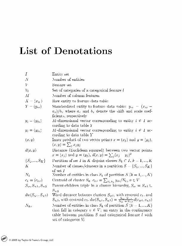
List of Denotations
I Entity set
N Number of entities
V Feature set
Vl Set of categories of a categorical feature l
M Number of column features
X � �xiv� Raw entitytofeature data table
Y � �yiv� Standardized entitytofeature data table� yiv � �xiv �av��bv where av and bv denote the shift and scale coef�cients� respectively
yi � �yiv� M dimensional vector corresponding to entity i � I according to data table Y
yi � �yiv� M dimensional vector corresponding to entity i � I according to data table Y
�x� y� Inner product of two vector points x � �xj� and y � �yj���x� y� �
Pj xjyj
d�x� y� Distance �Euclidean squared� between two vector pointsx � �xj� and y � �yj�� d�x� y� �
Pj�xj � yj�
�
fS�� ���� SKg Partition of set I in K disjoint classes Sk � I � k � �� ����K
K Number of classes�clusters in a partition S � fS�� ���� SKgof set I
Nk Number of entities in class Sk of partition S �k � �� ����K�
ck � �ckv� Centroid of cluster Sk� ckv �P
i�Skyiv�Nk� v � V
Sw� Sw�� Sw� Parentchildren triple in a cluster hierarchy� Sw � Sw� �Sw�
dw�Sw�� Sw�� Ward distance between clusters Sw�� with centroid c�� andSw�� with centroid c�� dw�Sw�� Sw�� � Nw�Nw�
Nw��Nw�d�cw�� cw��
Nkv Number of entities in class Sk of partition S �k � �� ����K�that fall in category v � V � an entry in the contingencytable between partition S and categorical feature l withset of categories Vl
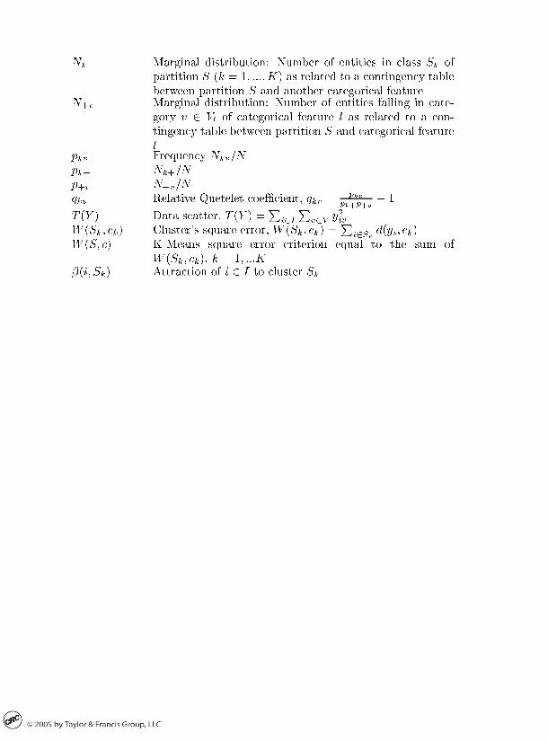
Nk� Marginal distribution� Number of entities in class Sk ofpartition S �k � �� ����K� as related to a contingency tablebetween partition S and another categorical feature
N�v Marginal distribution� Number of entities falling in category v � Vl of categorical feature l as related to a contingency table between partition S and categorical featurel
pkv Frequency Nkv�Npk� Nk��Np�v N�v�Nqkv Relative Quetelet coe�cient� qkv � pkv
pk�p�v� �
T �Y � Data scatter� T �Y � �P
i�I
Pv�V y�iv
W �Sk� ck� Cluster�s square error� W �Sk� ck� �P
i�Skd�yi� ck�
W �S� c� KMeans square error criterion equal to the sum ofW �Sk� ck�� k � �� ���K
��i� Sk� Attraction of i � I to cluster Sk
Introduction� Historical
Remarks
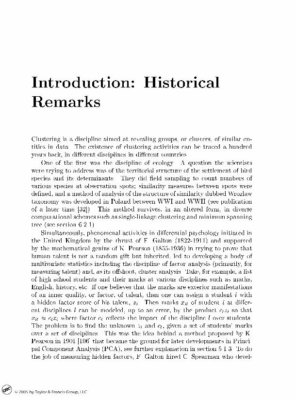
Clustering is a discipline aimed at revealing groups� or clusters� of similar entities in data� The existence of clustering activities can be traced a hundredyears back� in di�erent disciplines in di�erent countries�
One of the �rst was the discipline of ecology� A question the scientistswere trying to address was of the territorial structure of the settlement of birdspecies and its determinants� They did �eld sampling to count numbers ofvarious species at observation spots� similarity measures between spots werede�ned� and a method of analysis of the structure of similarity dubbed Wrozlawtaxonomy was developed in Poland between WWI and WWII �see publicationof a later time ������ This method survives� in an altered form� in diversecomputational schemes such as singlelinkage clustering and minimum spanningtree �see section ������
Simultaneously� phenomenal activities in di�erential psychology initiated inthe United Kingdom by the thrust of F� Galton ���������� and supportedby the mathematical genius of K� Pearson ��������� in trying to prove thathuman talent is not a random gift but inherited� led to developing a body ofmultivariate statistics including the discipline of factor analysis �primarily� formeasuring talent� and� as its o�shoot� cluster analysis� Take� for example� a listof high school students and their marks at various disciplines such as maths�English� history� etc� If one believes that the marks are exterior manifestationsof an inner quality� or factor� of talent� then one can assign a student i witha hidden factor score of his talent� zi� Then marks xil of student i at di�erent disciplines l can be modeled� up to an error� by the product clzi so thatxil � clzi where factor cl re�ects the impact of the discipline l over students�The problem is to �nd the unknown zi and cl� given a set of students� marksover a set of disciplines� This was the idea behind a method proposed by K�Pearson in �� � �� � that became the ground for later developments in Principal Component Analysis �PCA�� see further explanation in section ������ To dothe job of measuring hidden factors� F� Galton hired C� Spearman who devel
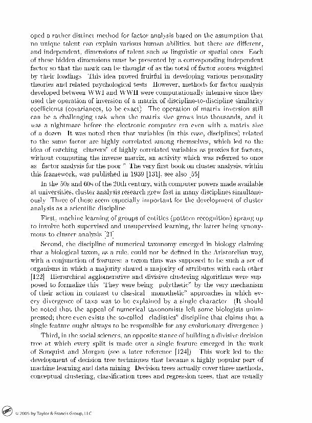
oped a rather distinct method for factor analysis based on the assumption thatno unique talent can explain various human abilities� but there are di�erent�and independent� dimensions of talent such as linguistic or spatial ones� Eachof these hidden dimensions must be presented by a corresponding independentfactor so that the mark can be thought of as the total of factor scores weightedby their loadings� This idea proved fruitful in developing various personalitytheories and related psychological tests� However� methods for factor analysisdeveloped between WWI and WWII were computationally intensive since theyused the operation of inversion of a matrix of disciplinetodiscipline similaritycoe�cients �covariances� to be exact�� The operation of matrix inversion stillcan be a challenging task when the matrix size grows into thousands� and itwas a nightmare before the electronic computer era even with a matrix sizeof a dozen� It was noted then that variables �in this case� disciplines� relatedto the same factor are highly correlated among themselves� which led to theidea of catching �clusters� of highly correlated variables as proxies for factors�without computing the inverse matrix� an activity which was referred to onceas �factor analysis for the poor�� The very �rst book on cluster analysis� withinthis framework� was published in ���� ������ see also �����
In the � s and s of the � th century� with computer powers made availableat universities� cluster analysis research grew fast in many disciplines simultaneously� Three of these seem especially important for the development of clusteranalysis as a scienti�c discipline�
First� machine learning of groups of entities �pattern recognition� sprang upto involve both supervised and unsupervised learning� the latter being synonymous to cluster analysis �����
Second� the discipline of numerical taxonomy emerged in biology claimingthat a biological taxon� as a rule� could not be de�ned in the Aristotelian way�with a conjunction of features� a taxon thus was supposed to be such a set oforganisms in which a majority shared a majority of attributes with each other������ Hierarchical agglomerative and divisive clustering algorithms were supposed to formalize this� They were being �polythetic� by the very mechanismof their action in contrast to classical �monothetic� approaches in which every divergence of taxa was to be explained by a single character� �It shouldbe noted that the appeal of numerical taxonomists left some biologists unimpressed� there even exists the socalled �cladistics� discipline that claims that asingle feature ought always to be responsible for any evolutionary divergence��
Third� in the social sciences� an opposite stance of building a divisive decisiontree at which every split is made over a single feature emerged in the workof Sonquist and Morgan �see a later reference ������� This work led to thedevelopment of decision tree techniques that became a highly popular part ofmachine learning and data mining� Decision trees actually cover three methods�conceptual clustering� classi�cation trees and regression trees� that are usually
considered di�erent because they employ di�erent criteria of homogeneity �����In a conceptual clustering tree� split parts must be as homogeneous as possiblewith regard to all participating features� In contrast� a classi�cation tree orregression tree achieves homogeneity with regard to only one� socalled target�feature� Still� we consider that all these techniques belong in cluster analysisbecause they all produce split parts consisting of similar entities� however� thisdoes not prevent them also being part of other disciplines such as machinelearning or pattern recognition�
A number of books re�ecting these developments were published in the � sdescribing the great opportunities opened in many areas of human activity byalgorithms for �nding �coherent� clusters in a data �cloud� placed in geometrical space �see� for example� Benz�ecri ����� Bock ����� Cli�ord and Stephenson����� Duda and Hart ����� Duran and Odell ����� Everitt ����� Hartigan �����Sneath and Sokal ����� Sonquist� Baker� and Morgan ����� Van Ryzin �����Zagoruyko ������ In the next decade� some of these developments have beenfurther advanced and presented in such books as Breiman et al� ����� Jain andDubes ���� and McLachlan and Basford ����� Still the common view is that clustering is an art rather than a science because determining clusters may dependmore on the user�s goals than on a theory� Accordingly� clustering is viewed asa set of diverse and ad hoc procedures rather than a consistent theory�
The last decade saw the emergence of data mining� the discipline combiningissues of handling and maintaining data with approaches from statistics andmachine learning for discovering patterns in data� In contrast to the statisticalapproach� which tries to �nd and �t objective regularities in data� data miningis oriented towards the end user� That means that data mining considers theproblem of useful knowledge discovery in its entire range� starting from databaseacquisition to data preprocessing to �nding patterns to drawing conclusions� Inparticular� the concept of an interesting pattern as something which is unusualor far from normal or anomalous has been introduced into data mining �����Obviously� an anomalous cluster is one that is further away from the grandmean or any other point of reference � an approach which is adapted in thistext�
A number of computer programs for carrying out data mining tasks� clustering included� have been successfully exploited� both in science and industry�a review of them can be found in ����� There are a number of general purposestatistical packages which have made it through from earlier times� those withsome cluster analysis applications such as SAS ����� and SPSS���� or those entirely devoted to clustering such as CLUSTAN ��� �� There are data miningtools which include clustering� such as Clementine ����� Still� these programsare far from su�cient in advising a user on what method to select� how topreprocess data and� especially� what sense to make of the clusters�
Another feature of this more recent period is that a number of application
areas have emerged in which clustering is a key issue� In many applicationareas that began much earlier � such as image analysis� machine vision or robotplanning � clustering is a rather small part of a very complex task such thatthe quality of clustering does not much matter to the overall performance� asany reasonable heuristic would do� these areas do not require the discipline ofclustering to theoretically develop and mature�
This is not so in Bioinformatics� the discipline which tries to make senseof interrelation between structure� function and evolution of biomolecular objects� Its primary entities� DNA and protein sequences� are complex enoughto have their similarity modeled as homology� that is� inheritance from a common ancestor� More advanced structural data such as protein folds and theircontact maps are being constantly added to existing depositories� Gene expression technologies add to this an invaluable next step a wealth of data onbiomolecular function� Clustering is one of the major tools in the analysis ofbioinformatics data� The very nature of the problem here makes researcherssee clustering as a tool not only for �nding cohesive groupings in data but alsofor relating the aspects of structure� function and evolution to each other� Inthis way� clustering is more and more becoming part of an emerging area ofcomputer classi�cation� It models the major functions of classi�cation in thesciences� the structuring of a phenomenon and associating its di�erent aspects��Though� in data mining� the term classi�cation� is almost exclusively usedin its partial meaning as merely a diagnostic tool�� Theoretical and practicalresearch in clustering is thriving in this area�
Another area of booming clustering research is information retrieval and textdocument mining� With the growth of the Internet and the World Wide Web�text has become one of the most important mediums of mass communication�The terabytes of text that exist must be summarized e�ectively� which involvesa great deal of clustering in such key stages as natural language processing�feature extraction� categorization� annotation and summarization� In author�sview� clustering will become even more important as the systems for acquiringand understanding knowledge from texts evolve� which is likely to occur soon�There are already web sites providing web search results with clustering themaccording to automatically found key phrases �see� for instance� �������
This book is mostly devoted to explaining and extending two clusteringtechniques� KMeans for partitioning and Ward for hierarchical clustering� Thechoice is far from random� First� they present the most popular clusteringformats� hierarchies and partitions� and can be extended to other interestingformats such as single clusters� Second� many other clustering and statisticaltechniques� such as conceptual clustering� selforganizing maps �SOM�� andcontingency association measures� appear to be closely related to these� Third�both methods involve the same criterion� the minimum within cluster variance�which can be treated within the same theoretical framework� Fourth� many data
mining issues of current interest� such as analysis of mixed data� incompleteclustering� and conceptual description of clusters� can be treated with extendedversions of these methods� In fact� the book contents go far beyond thesemethods� the two last chapters� accounting for one third of the material� aredevoted to the �big issues� in clustering and data mining that are not limitedto speci�c methods�
The present account of the methods is based on a speci�c approach to cluster analysis� which can be referred to as the data recovery clustering� In thisapproach� clusters are not only found in data but they also feed back into thedata� a cluster structure is used to generate data in the format of the datatable which has been analyzed with clustering� The data generated by a clusterstructure are� in a sense� �ideal� as they reproduce only the cluster structurelying behind their generation� The observed data can then be considered anoisy version of the ideal clustergenerated data� the extent of noise can bemeasured by the di�erence between the ideal and observed data� The smallerthe di�erence the better the �t� This idea is not particularly new� it is� in fact�the backbone of many quantitative methods of multivariate statistics� such asregression and factor analysis� Moreover� it has been applied in clustering fromthe very beginning� in particular� Ward ����� developed his method of agglomerative clustering with implicitly this view of data analysis� Some methodswere consciously constructed along the data recovery approach� see� for instance� work of Hartigan ��� at which the single linkage method was developedto approximate the data with an ultrametric matrix� an ideal data type corresponding to a cluster hierarchy� Even more appealing in this capacity is a laterwork by Hartigan �����
However� this approach has never been applied in full� The sheer idea� following from models presented in this book� that classical clustering is but aconstrained analogue to the principal component model has not achieved anypopularity so far� though it has been around for quite a while ����� �� �� Theunifying capability of the data recovery clustering is grounded on convenientrelations which exist between data approximation problems and geometricallyexplicit classical clustering� Firm mathematical relations found between different parts of cluster solutions and data lead not only to explanation of theclassical algorithms but also to development of a number of other algorithms forboth �nding and describing clusters� Among the former� principalcomponentlike algorithms for �nding anomalous clusters and divisive clustering should bepointed out� Among the latter� a set of simple but e�cient interpretation tools�that are absent from the multiple programs implementing classical clusteringmethods� should be mentioned�
Chapter �
What Is Clustering
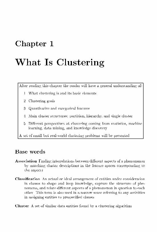
After reading this chapter the reader will have a general understanding of�
�� What clustering is and its basic elements�
�� Clustering goals�
�� Quantitative and categorical features�
�� Main cluster structures� partition� hierarchy� and single cluster�
�� Di erent perspectives at clustering coming from statistics� machinelearning� data mining� and knowledge discovery�
A set of small but realworld clustering problems will be presented�
Base words
Association Finding interrelations between di erent aspects of a phenomenonby matching cluster descriptions in the feature spaces corresponding tothe aspects�
Classi�cation An actual or ideal arrangement of entities under considerationin classes to shape and keep knowledge� capture the structure of phenomena� and relate di erent aspects of a phenomenon in question to eachother� This term is also used in a narrow sense referring to any activitiesin assigning entities to prespecied classes�
Cluster A set of similar data entities found by a clustering algorithm�

� WHAT IS CLUSTERING
Cluster representative An element of a cluster to represent its �typical�properties� This is used for cluster description in domains knowledge ofwhich is poor�
Cluster structure A representation of an entity set I as a set of clusters thatform either a partition of I or hierarchy on I or an incomplete clusteringof I �
Cluster tendency A description of a cluster in terms of the average values ofrelevant features�
Clustering An activity of nding and�or describing cluster structures in adata set�
Clustering goal Types of problems of data analysis to which clustering can beapplied� associating� structuring� describing� generalizing and visualizing�
Clustering criterion A formal denition or scoring function that can be usedin computational algorithms for clustering�
Conceptual description A logical statement characterizing a cluster or cluster structure in terms of relevant features�
Data A set of entities characterized by values of quantitative or categoricalfeatures� Sometimes data may characterize relations between entities suchas similarity coe�cients or transaction �ows�
Data mining perspective In data mining� clustering is a tool for ndingpatterns and regularities within the data�
Generalization Making general statements about data and� potentially� aboutthe phenomenon the data relate to�
Knowledge discovery perspective In knowledge discovery� clustering is atool for updating� correcting and extending the existing knowledge� Inthis regard� clustering is but empirical classication�
Machine learning perspective In machine learning� clustering is a tool forprediction�
Statistics perspective In statistics� clustering is a method to t a prespecied probabilistic model of the data generating mechanism�
Structuring Representing data with a cluster structure�
Visualization Mapping data onto a known �ground� image such as the coordinate plane or a genealogy tree � in such a way that properties of thedata are re�ected in the structure of the ground image�
���� EXEMPLARY PROBLEMS �
��� Exemplary problems
Clustering is a discipline devoted to revealing and describing homogeneousgroups of entities� that is� clusters� in data sets� Why would one need this�Here is a list of potentially overlapping objectives for clustering�
�� Structuring� that is� representing data as a set of groups of similar objects�
�� Description of clusters in terms of features� not necessarily involved innding the clusters�
�� Association� that is� nding interrelations between di erent aspects of aphenomenon by matching cluster descriptions in spaces corresponding tothe aspects�
�� Generalization� that is� making general statements about data and�potentially� the phenomena the data relate to�
�� Visualization� that is� representing cluster structures as visual images�
These categories are not mutually exclusive� nor do they cover the entire range ofclustering goals but rather re�ect the author�s opinion on the main applicationsof clustering� In the remainder of this section we provide realworld examples ofdata and the related clustering problems for each of these goals� For illustrativepurposes� small data sets are used in order to provide the reader with theopportunity of directly observing further processing with the naked eye�
����� Structuring
Structuring is the main goal of many clustering applications� which is to ndprincipal groups of entities in their specics� The cluster structure of an entityset can be looked at through di erent glasses� One user may wish to aggregatethe set in a system of nonoverlapping classes� another user may prefer to developa taxonomy as a hierarchy of more and more abstract concepts� yet another usermay wish to focus on a cluster of �core� entities considering the rest as merelya nuisance� These are conceptualized in di erent types of cluster structures�such as a partition� a hierarchy� or a single subset�
Market towns
Table ��� represents a small portion of a list of thirteen hundred English markettowns characterized by the population and services provided in each listed inthe following box�
� WHAT IS CLUSTERING
Market town features�
P Population resident in ���� Census
PS Primary Schools
Do Doctor Surgeries
Ho Hospitals
Ba Banks and Building Societies
SM National Chain Supermarkets
Pe Petrol Stations
DIY DoItYourself Shops
SP Public Swimming Pools
PO Post O�ces
CA Citizen�s Advice Bureaux �cheap legal advice�
FM Farmers� Markets
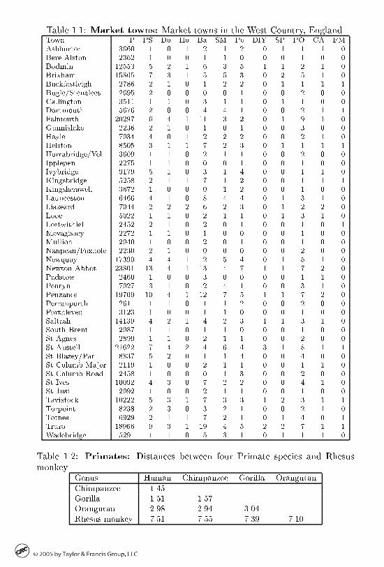
For the purposes of social monitoring� the set of all market towns should bepartitioned into similarity clusters in such a way that a representative from eachof the clusters may be utilized as a unit of observation� Those characteristicsof the clusters that separate them from the others should be used to properlyselect representative towns�
As further computations will show� the numbers of services on average follow the town sizes� so that the found clusters can be described mainly in termsof the population size� This set� as well as the complete set of almost thirteenhundred English market towns� consists of seven clusters that can be describedas belonging to four tiers of population� large towns of about �������� inhabitants� two clusters of medium sized towns �������� inhabitants�� three clustersof small towns �about ����� inhabitants� and a cluster of very small settlementswith about ����� inhabitants� The di erence between clusters in the same population tier is caused by the presence or absence of some service features� Forinstance� each of the three small town clusters is characterized by the presenceof a facility� which is absent in two others� a Farm market� a Hospital anda Swimming pool� respectively� The number of clusters is determined in theprocess of computations �see sections ���� �������
This data set is analyzed on pp� ��� ��� ��� ��� ��� ��� ��� ���� ���� ����
Primates and Human origin
In Table ���� the data on genetic distances between Human and three genera ofgreat apes are presented� the Rhesus monkey is added as a distant relative tocertify the starting divergence event� It is well established that humans divergedfrom a common ancestor with chimpanzees approximately � million years ago�after a divergence from other great apes� Let us see how compatible with thisconclusion the results of cluster analysis are�
���� EXEMPLARY PROBLEMS �
Table ���� Market towns� Market towns in the West Country� England�Town P PS Do Ho Ba SM Pe DIY SP PO CA FMAshburton ���� � � � � � � � � � � �Bere Alston ���� � � � � � � � � � � �Bodmin ����� � � � � � � � � � � �Brixham ����� � � � � � � � � � � �Buckfastleigh ���� � � � � � � � � � � �Bugle�Stenalees ��� � � � � � � � � � � �Callington ���� � � � � � � � � � � �Dartmouth ���� � � � � � � � � �Falmouth ���� � � �� � � � � � �Gunnislake ���� � � � � � � � � � � �Hayle ��� � � � � � � � � � �Helston ���� � � � � � � � � � � �Horrabridge�Yel ��� � � � � � � � � � � �Ipplepen ���� � � � � � � � � � � �Ivybridge �� � � � � � � � � � �Kingsbridge ���� � � � � � � � � � � �Kingskerswell ���� � � � � � � � � � � �Launceston ��� � � � � � � � �Liskeard �� � � � � � � � � � � �Looe ���� � � � � � � � � � � �Lostwithiel ��� � � � � � � � � � � �Mevagissey ���� � � � � � � � � � � �Mullion ��� � � � � � � � � � � �Nanpean�Foxhole ���� � � � � � � � � � � �Newquay ���� � �� � � � � � �Newton Abbot ����� �� � �� � � � � � �Padstow ��� � � � � � � � � � � �Penryn ���� � � � � � � � � � �Penzance ��� �� � �� � � � � � � �Perranporth ���� � � � � � � � � � � �Porthleven ���� � � � � � � � � � � �Saltash ��� � � � � � � � � �South Brent ���� � � � � � � � � � � �St Agnes �� � � � � � � � � � � �St Austell ����� � � � � � � � � �St Blazey�Par ���� � � � � � � � � �St Columb Major ��� � � � � � � � � � � �St Columb Road ��� � � � � � � � � � � �St Ives ���� � � � � � � � � �St Just ��� � � � � � � � � � � �Tavistock ����� � � � � � � � � � � �Torpoint ���� � � � � � � � � � � �Totnes �� � � � � � � � � � �Truro ���� � � � � � � � � �Wadebridge ��� � � � � � � � � � � �
Table ���� Primates� Distances between four Primate species and Rhesusmonkey�
Genus Human Chimpanzee Gorilla Orangutan
Chimpanzee ����Gorilla ���� ����Orangutan ���� ���� ���Rhesus monkey ���� ���� ���� ���
� WHAT IS CLUSTERING
RhM Ora Chim Hum Gor
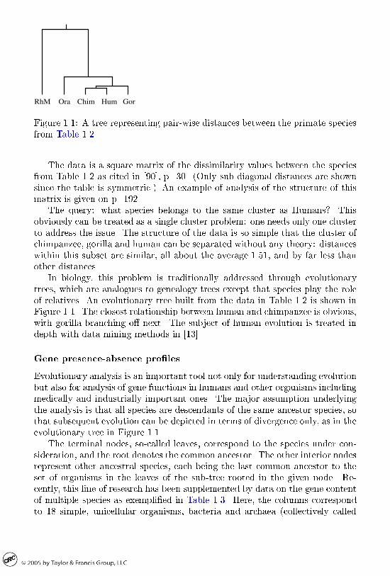
Figure ���� A tree representing pairwise distances between the primate speciesfrom Table ����
The data is a square matrix of the dissimilarity values between the speciesfrom Table ��� as cited in ����� p� ��� �Only subdiagonal distances are shownsince the table is symmetric�� An example of analysis of the structure of thismatrix is given on p� ����The query� what species belongs to the same cluster as Humans� This
obviously can be treated as a single cluster problem� one needs only one clusterto address the issue� The structure of the data is so simple that the cluster ofchimpanzee� gorilla and human can be separated without any theory� distanceswithin this subset are similar� all about the average ����� and by far less thanother distances�In biology� this problem is traditionally addressed through evolutionary
trees� which are analogues to genealogy trees except that species play the roleof relatives� An evolutionary tree built from the data in Table ��� is shown inFigure ���� The closest relationship between human and chimpanzee is obvious�with gorilla branching o next� The subject of human evolution is treated indepth with data mining methods in �����
Gene presence�absence pro�les
Evolutionary analysis is an important tool not only for understanding evolutionbut also for analysis of gene functions in humans and other organisms includingmedically and industrially important ones� The major assumption underlyingthe analysis is that all species are descendants of the same ancestor species� sothat subsequent evolution can be depicted in terms of divergence only� as in theevolutionary tree in Figure ����The terminal nodes� socalled leaves� correspond to the species under con
sideration� and the root denotes the common ancestor� The other interior nodesrepresent other ancestral species� each being the last common ancestor to theset of organisms in the leaves of the subtree rooted in the given node� Recently� this line of research has been supplemented by data on the gene contentof multiple species as exemplied in Table ���� Here� the columns correspondto �� simple� unicellular organisms� bacteria and archaea �collectively called
���� EXEMPLARY PROBLEMS �
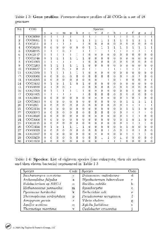
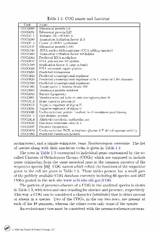
Table ���� Gene pro�les� Presenceabsence proles of �� COGs in a set of ��genomes�
No COG Speciesy a o m p k z q v d r b c e f g s j
� COG��� � � � � � � � � � � � � � � � � � �� COG��� � � � � � � � � � � � � � � � � � �� COG���� � � � � � � � � � � � � � � � � � � COG��� � � � � � � � � � � � � � � � � � �� COG���� � � � � � � � � � � � � � � � � � �� COG��� � � � � � � � � � � � � � � � � � �� COG��� � � � � � � � � � � � � � � � � � �� COG��� � � � � � � � � � � � � � � � � � � COG���� � � � � � � � � � � � � � � � � � ��� COG��� � � � � � � � � � � � � � � � � � ��� COG�� � � � � � � � � � � � � � � � � � ��� COG���� � � � � � � � � � � � � � � � � � ��� COG��� � � � � � � � � � � � � � � � � � �� COG��� � � � � � � � � � � � � � � � � � ��� COG���� � � � � � � � � � � � � � � � � � ��� COG��� � � � � � � � � � � � � � � � � � ��� COG��� � � � � � � � � � � � � � � � � � ��� COG��� � � � � � � � � � � � � � � � � � �� COG���� � � � � � � � � � � � � � � � � � ��� COG��� � � � � � � � � � � � � � � � � � ��� COG��� � � � � � � � � � � � � � � � � � ��� COG���� � � � � � � � � � � � � � � � � � ��� COG���� � � � � � � � � � � � � � � � � � �� COG���� � � � � � � � � � � � � � � � � � ��� COG���� � � � � � � � � � � � � � � � � � ��� COG�� � � � � � � � � � � � � � � � � � ��� COG��� � � � � � � � � � � � � � � � � � ��� COG���� � � � � � � � � � � � � � � � � � �� COG�� � � � � � � � � � � � � � � � � � ��� COG��� � � � � � � � � � � � � � � � � � �
Table ���� Species� List of eighteen species �one eukaryota� then six archaeaand then eleven bacteria� represented in Table ����
Species Code Species Code
Saccharomyces cerevisiae y Deinococcus radiodurans dArchaeoglobus fulgidus a Mycobacterium tuberculosis rHalobacterium sp�NRC�� o Bacillus subtilis bMethanococcus jannaschii m Synechocystis cPyrococcus horikoshii k Escherichia coli eThermoplasma acidophilum p Pseudomonas aeruginosa fAeropyrum pernix z Vibrio cholera gAquifex aeolicus q Xylella fastidiosa sThermotoga maritima v Caulobacter crescentus j
� WHAT IS CLUSTERING
Table ���� COG names and functions�
Code NameCOG��� Ribosomal protein L�COG��� Ribosomal protein L��COG���� Archaeal Glu�tRNAGlnCOG��� Translation initiation factor IF�COG���� Cysteinyl�tRNA synthetaseCOG��� Ribosomal protein L�ECOG��� tRNA nucleotidyltransferase �CCA�adding enzyme COG��� Translation initiation factor eIF�alphaCOG���� Predicted RNA methylaseCOG��� DNA polymerase III epsilonCOG�� Replication factor A large subunitCOG���� DNA mismatch repair proteinCOG��� Predicted transposaseCOG��� Predicted transcriptional regulatorCOG���� Predicted transcriptional regulator with C�terminal CBS domainsCOG��� Predicted transcriptional regulatorsCOG��� Transcription initiation factor IIBCOG��� Membrane protein involvedCOG���� Surface lipoproteinCOG��� Membrane�bound lytic murein transglycosylase BCOG��� Heme exporter protein DCOG���� Negative regulator of sigma ECOG���� Negative regulator of sigma ECOG���� Uncharacterized protein involved in chromosome partitioningCOG���� Cell division proteinCOG�� Aldehyde�ferredoxin oxidoreductaseCOG��� Fumarate reductase subunit CCOG���� Putative lipoproteinCOG�� Uncharacterized BCR� stimulates glucose���P dehydrogenase activityCOG��� Predicted membrane protein
prokaryotes�� and a simple eukaryote� yeast Saccharomyces cerevisiae� The listof species along with their oneletter codes is given in Table ����
The rows in Table ��� correspond to individual genes represented by the socalled Clusters of Orthologous Groups �COGs� which are supposed to includegenes originating from the same ancestral gene in the common ancestor of therespective species ����� COG names which re�ect the functions of the respectivegenes in the cell are given in Table ���� These tables present but a small partof the publicly available COG database currently including �� species and ����COGs posted in the web site www�ncbi�nlm�nih�gov�COG�
The pattern of presenceabsence of a COG in the analyzed species is shownin Table ���� with zeros and ones standing for absence and presence� respectively�This way� a COG can be considered a character �attribute� that is either presentor absent in a species� Two of the COGs� in the top two rows� are present ateach of the �� genomes� whereas the others cover only some of the species�
An evolutionary tree must be consistent with the presenceabsence patterns�

���� EXEMPLARY PROBLEMS �
Specically� if a COG is present in two species� then it should be present in theirlast common ancestor and� thus� in all other descendants of the last commonancestor� This would be in accord with the natural process of inheritance�However� in most cases� the presenceabsence pattern of a COG in extant speciesis far from the �natural� one� many genes are dispersed over several subtrees�According to comparative genomics� this may happen because of multiple lossand horizontal transfer of genes ����� The hierarchy should be constructed insuch a way that the number of inconsistencies is minimized�
The socalled principle of Maximum Parsimony �MP� is a straightforwardformalization of this idea� Unfortunately� MP does not always lead to appropriate solutions because of intrinsic and computational problems� A numberof other approaches have been proposed including hierarchical cluster analysis�see �������
Especially appealing in this regard is divisive cluster analysis� It begins bysplitting the entire data set into two parts� thus imitating the divergence ofthe last universal common ancestor �LUCA� into two descendants� The sameprocess then applies to each of the split parts until a stopcriterion is reached tohalt the division process� In contrast to other methods for building evolutionary trees� divisive clustering imitates the process of evolutionary divergence�Further approximation of the real evolutionary process can be achieved if thecharacters on which divergence is based are discarded immediately after thedivision of the respective cluster ����� Gene proles data are analyzed on p���� and p� ����
After an evolutionary tree is built� it can be utilized for reconstructing genehistories by mapping events of emergence� inheritance� loss and horizontal transfer of individual COGs on the tree according to the principle of MaximumParsimony �see p� ����� These histories of individual genes can be helpful inadvancing our understanding of biological functions and drug design�
����� Description
The problem of description is that of automatically deriving a conceptual description of clusters found by a clustering algorithm or supplied from a di erentsource� The problem of cluster description belongs in cluster analysis becausethis is part of the interpretation and understanding of clusters� A good conceptual description can be used for better understanding and�or better predicting�The latter because we can check whether an object in question satises thedescription or not� the more the object satises the description the better thechances that it belongs to the cluster described� This is why conceptual description tools� such as decision trees ���� ���� have been conveniently used anddeveloped mostly for the purposes of prediction�
�� WHAT IS CLUSTERING
Describing Iris genera
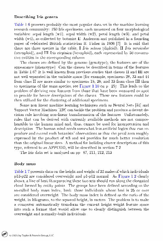
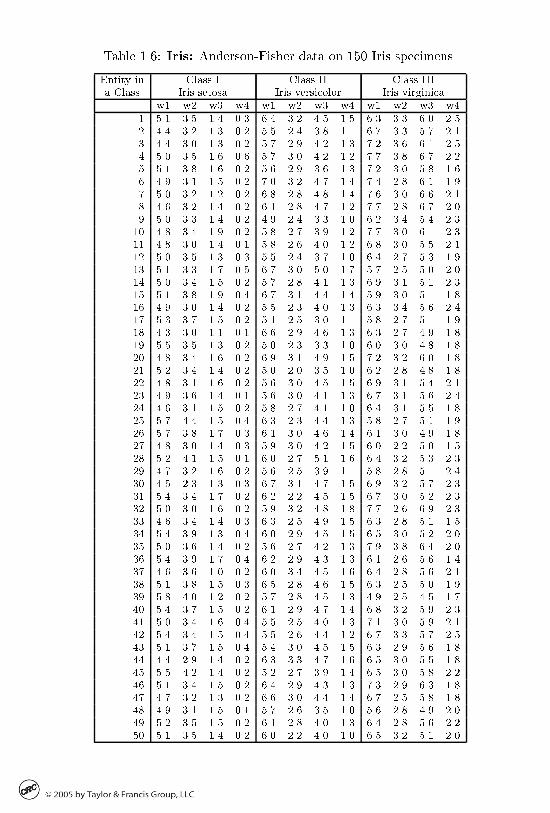
Table ��� presents probably the most popular data set in the machine learningresearch community� ��� Iris specimens� each measured on four morphologicalvariables� sepal length �w��� sepal width �w��� petal length �w��� and petalwidth �w��� as collected by botanist E� Anderson and published in a foundingpaper of celebrated British statistician R� Fisher in ���� ���� It is said thatthere are three species in the table� I Iris setosa �diploid�� II Iris versicolor�tetraploid�� and III Iris virginica �hexaploid�� each represented by �� consecutive entities in the corresponding column�
The classes are dened by the genome �genotype�� the features are of theappearance �phenotype�� Can the classes be described in terms of the featuresin Table ���� It is well known from previous studies that classes II and III arenot well separated in the variable space �for example� specimens ��� �� and ��from class II are more similar to specimens ��� ��� and �� from class III thanto specimens of the same species� see Figure ���� on p� ���� This leads to theproblem of deriving new features from those that have been measured on spotto provide for better descriptions of the classes� These new features could bethen utilized for the clustering of additional specimens�
Some nonlinear machine learning techniques such as Neural Nets ���� andSupport Vector Machines ����� can tackle the problem and produce a decent decision rule involving nonlinear transformation of the features� Unfortunately�rules that can be derived with currently available methods are not comprehensible to the human mind and� thus� cannot be used for interpretation anddescription� The human mind needs somewhat less articial logics that can reproduce and extend such botanists� observations as that the petal area roughlyexpressed by the product of w� and w� provides for much better resolutionthan the original linear sizes� A method for building cluster descriptions of thistype� referred to as APPCOD� will be described in section ����
The Iris data set is analyzed on pp� ��� ���� ���� ����
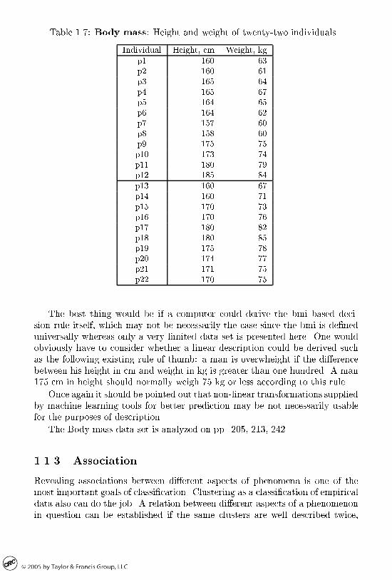
Body mass
Table ��� presents data on the height and weight of �� males of which individualsp��p�� are considered overweight and p�p�� normal� As Figure ��� clearlyshows� a line of best t separating these two sets should run along the elongatedcloud formed by entity points� The groups have been dened according to thesocalled body mass index� bmi� those individuals whose bmi is �� or overare considered overweight� The body mass index is dened as the ratio of theweight� in kilograms� to the squared height� in meters� The problem is to makea computer automatically transform the current heightweight feature spaceinto such a format that would allow one to clearly distinguish between theoverweight and normallybuilt individuals�
���� EXEMPLARY PROBLEMS ��
Table ���� Iris� AndersonFisher data on ��� Iris specimens�
Entity in Class I Class II Class IIIa Class Iris setosa Iris versicolor Iris virginica
w� w� w� w w� w� w� w w� w� w� w� ��� ��� �� ��� �� ��� �� ��� ��� ��� ��� ���� � ��� ��� ��� ��� �� ��� ��� ��� ��� ��� ���� � ��� ��� ��� ��� �� �� ��� ��� ��� ��� ��� ��� ��� ��� ��� ��� ��� �� ��� ��� ��� ��� ���� ��� ��� ��� ��� ��� �� ��� ��� ��� ��� ��� ���� � ��� ��� ��� ��� ��� �� �� �� ��� ��� ��� ��� ��� ��� ��� ��� ��� �� �� ��� ��� ��� ���� �� ��� �� ��� ��� ��� �� ��� ��� ��� ��� ��� ��� ��� �� ��� � �� ��� ��� ��� �� �� ����� �� �� �� ��� ��� ��� �� ��� ��� ��� ��� ����� �� ��� �� ��� ��� ��� �� ��� ��� ��� ��� ����� ��� ��� ��� ��� ��� �� ��� ��� �� ��� ��� ���� ��� ��� ��� ��� ��� ��� ��� ��� ��� ��� ��� ���� ��� �� ��� ��� ��� ��� �� ��� �� ��� ��� ����� ��� ��� �� �� ��� ��� � �� �� ��� ��� ����� � ��� �� ��� ��� ��� �� ��� ��� �� ��� ���� ��� ��� ��� ��� ��� ��� ��� ��� ��� ��� ��� ���� �� ��� ��� ��� ��� �� �� ��� ��� ��� � ���� ��� ��� ��� ��� ��� ��� ��� ��� ��� ��� �� ����� �� �� ��� ��� �� ��� � ��� ��� ��� ��� ����� ��� �� �� ��� ��� ��� ��� ��� ��� ��� �� ����� �� ��� ��� ��� ��� ��� �� ��� �� ��� �� ����� � ��� �� ��� ��� ��� �� ��� ��� ��� ��� ��� �� ��� ��� ��� ��� ��� �� ��� �� ��� ��� ����� ��� � ��� �� ��� ��� � ��� ��� ��� ��� ���� ��� ��� ��� ��� ��� ��� �� �� ��� ��� � ����� �� ��� �� ��� �� ��� �� ��� ��� ��� ��� ����� ��� �� ��� ��� ��� ��� ��� ��� �� ��� ��� ���� �� ��� ��� ��� ��� ��� �� ��� ��� ��� ��� ���� �� ��� ��� ��� ��� ��� �� ��� �� ��� ��� ����� �� �� ��� ��� ��� ��� �� ��� ��� ��� ��� ����� ��� ��� ��� ��� �� ��� �� ��� ��� ��� �� ����� �� �� �� ��� ��� ��� � ��� ��� ��� ��� ���� �� �� ��� �� ��� �� �� ��� ��� ��� ��� ����� ��� ��� �� ��� ��� ��� �� ��� �� ��� �� ����� �� �� ��� �� ��� �� �� ��� ��� ��� ��� ���� �� ��� ��� ��� ��� �� �� ��� �� ��� ��� ����� ��� ��� ��� ��� ��� ��� �� ��� ��� ��� ��� ��� ��� �� ��� ��� ��� ��� �� ��� � ��� �� ���� �� ��� ��� ��� ��� �� �� �� ��� ��� �� ���� ��� �� ��� �� ��� ��� �� ��� ��� ��� �� ���� �� �� ��� �� ��� ��� � ��� ��� ��� ��� ���� ��� ��� ��� �� �� ��� �� ��� ��� �� ��� ��� � �� �� ��� ��� ��� �� ��� ��� ��� ��� ���� ��� �� �� ��� ��� ��� �� �� ��� ��� ��� ���� ��� �� ��� ��� �� �� �� ��� ��� �� ��� ���� �� ��� ��� ��� ��� ��� � �� ��� ��� ��� ���� � ��� ��� ��� ��� ��� ��� ��� ��� ��� � ��� ��� ��� ��� ��� ��� ��� �� ��� �� ��� ��� ����� ��� ��� �� ��� ��� ��� �� ��� ��� ��� ��� ���
�� WHAT IS CLUSTERING
Table ���� Body mass� Height and weight of twentytwo individuals�
Individual Height cm Weight kg
p� �� ��p� �� ��p� ��� ��p� ��� ��p� ��� ��p� ��� ��p� ��� �p� ��� �p� ��� ��p� ��� ��p�� �� ��p�� ��� ��
p�� �� ��p�� �� ��p�� �� ��p�� �� ��p�� �� ��p�� �� ��p�� ��� ��p� ��� ��p�� ��� ��p�� �� ��
The best thing would be if a computer could derive the bmi based decision rule itself� which may not be necessarily the case since the bmi is deneduniversally whereas only a very limited data set is presented here� One wouldobviously have to consider whether a linear description could be derived suchas the following existing rule of thumb� a man is overwheight if the di erencebetween his height in cm and weight in kg is greater than one hundred� A man��� cm in height should normally weigh �� kg or less according to this rule�
Once again it should be pointed out that nonlinear transformations suppliedby machine learning tools for better prediction may be not necessarily usablefor the purposes of description�
The Body mass data set is analyzed on pp� ���� ���� ����
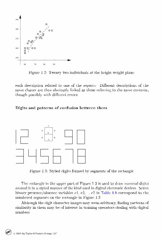
����� Association
Revealing associations between di erent aspects of phenomena is one of themost important goals of classication� Clustering as a classication of empiricaldata also can do the job� A relation between di erent aspects of a phenomenonin question can be established if the same clusters are well described twice�
���� EXEMPLARY PROBLEMS ��
60 70 80 90
150
160
170
180
190
Figure ���� Twentytwo individuals at the heightweight plane�
each description related to one of the aspects� Di erent descriptions of thesame cluster are then obviously linked as those referring to the same contents�though possibly with di erent errors�
Digits and patterns of confusion between them
1
2
5
3
67
4
Figure ���� Styled digits formed by segments of the rectangle�
The rectangle in the upper part of Figure ��� is used to draw numeral digitsaround it in a styled manner of the kind used in digital electronic devices� Sevenbinary presence�absence variables e�� e������ e� in Table ��� correspond to thenumbered segments on the rectangle in Figure ����
Although the digit character images may seem arbitrary� nding patterns ofsimilarity in them may be of interest in training operators dealing with digitalnumbers�

�� WHAT IS CLUSTERING
Table ���� Digits� Segmented numerals presented with seven binary variablescorresponding to presence�absence of the corresponding edge in Figure ����
Digit e� e� e� e�� e� e� e�� � � � � � � �� � � � � � � �� � � � � � � �� � � � � � � �� � � � � � � �� � � � � � � �� � � � � � � �� � � � � � � �� � � � � � � �� � � � � � � �
Table ���� Confusion� Confusion between the segmented numeral digits�
ResponseStimulus � � � � � � � � �
� ��� � � �� � �� � � �� �� ��� �� � �� �� �� �� � ��� �� �� ��� � �� � �� ��� ��� ��� �� � ��� � �� � � �� � �� �� �� �� ��� �� � � ��� ��� �� �� � �� �� ��� � ��� �� ��� ��� � �� �� � ��� � �� �� �� �� �� �� � �� ��� �� ���� �� �� ��� �� �� �� �� �� �� �� �� � � �� � �� �� �� �� ���
Results of a psychological experiment on confusion between the segmentednumerals are in Table ���� A digit appeared on a screen for a very short time�stimulus�� and an individual was asked to report what was the digit �response��The response frequencies of digits versus shown stimuli stand in the rows ofTable ��� �����
The problem is to nd general patterns in confusion and to interpret themin terms of the segment presenceabsence variables in Digits data Table ���� Ifthe found interpretation can be put in a theoretical framework� the patternscan be considered as empirical re�ections of theoretically substantiated classes�Patterns of confusion would show the structure of the phenomenon� Interpretation of the clusters in terms of the drawings� if successful� would allow us tosee what relation may exist between the patterns of drawing and confusion�
���� EXEMPLARY PROBLEMS ��
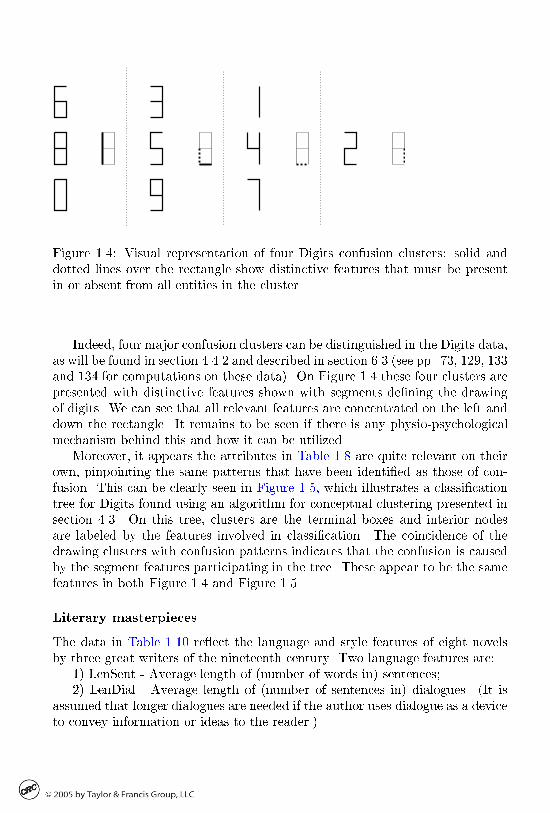
Figure ���� Visual representation of four Digits confusion clusters� solid anddotted lines over the rectangle show distinctive features that must be presentin or absent from all entities in the cluster�
Indeed� four major confusion clusters can be distinguished in the Digits data�as will be found in section ����� and described in section ��� �see pp� ��� ���� ���and ��� for computations on these data�� On Figure ��� these four clusters arepresented with distinctive features shown with segments dening the drawingof digits� We can see that all relevant features are concentrated on the left anddown the rectangle� It remains to be seen if there is any physiopsychologicalmechanism behind this and how it can be utilized�Moreover� it appears the attributes in Table ��� are quite relevant on their
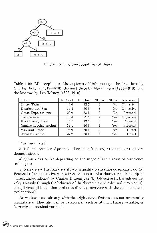
own� pinpointing the same patterns that have been identied as those of confusion� This can be clearly seen in Figure ���� which illustrates a classicationtree for Digits found using an algorithm for conceptual clustering presented insection ���� On this tree� clusters are the terminal boxes and interior nodesare labeled by the features involved in classication� The coincidence of thedrawing clusters with confusion patterns indicates that the confusion is causedby the segment features participating in the tree� These appear to be the samefeatures in both Figure ��� and Figure ����
Literary masterpieces
The data in Table ���� re�ect the language and style features of eight novelsby three great writers of the nineteenth century� Two language features are��� LenSent Average length of �number of words in� sentences��� LenDial Average length of �number of sentences in� dialogues� �It is
assumed that longer dialogues are needed if the author uses dialogue as a deviceto convey information or ideas to the reader��
�� WHAT IS CLUSTERING
2
1 0
1 0
6 8 0
3 5 9
1 4 7
e7
e5
e1
0 1
Figure ���� The conceptual tree of Digits�
Table ����� Masterpieces� Masterpieces of ��th century� the rst three byCharles Dickens ������������ the next three by Mark Twain ������������ andthe last two by Leo Tolstoy ������������
Title LenSent LenDial NChar SCon Narrative
Oliver Twist ��� ���� � No ObjectiveDombey and Son ���� ��� � No ObjectiveGreat Expectations ���� ��� � No Personal
Tom Sawyer ���� ���� � Yes ObjectiveHuckleberry Finn ���� ���� � Yes PersonalYankee at King Arthur ���� ���� � Yes Personal
War and Peace ���� ��� � Yes DirectAnna Karenina ���� ��� � Yes Direct
Features of style�
�� NChar Number of principal characters �the larger the number the morethemes raised��
�� SCon Yes or No depending on the usage of the stream of consciencetechniques�
�� Narrative The narrative style is a qualitative feature categorized as� �a�Personal �if the narrative comes from the mouth of a character such as Pip in�Great Expectations� by Charles Dickens�� or �b� Objective �if the subject develops mainly through the behavior of the characters and other indirect means��or �c� Direct �if the author prefers to directly intervene with the comments andexplanations��
As we have seen already with the Digits data� features are not necessarilyquantitative� They also can be categorical� such as SCon� a binary variable� orNarrative� a nominal variable�
���� EXEMPLARY PROBLEMS ��
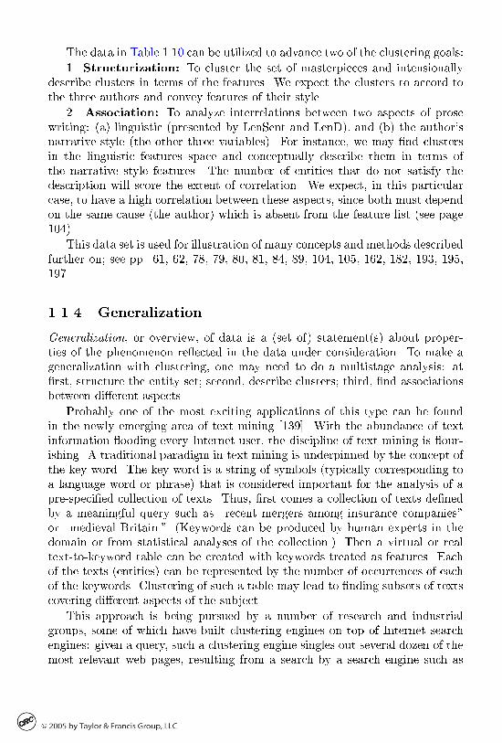
The data in Table ���� can be utilized to advance two of the clustering goals�
�� Structurization� To cluster the set of masterpieces and intensionallydescribe clusters in terms of the features� We expect the clusters to accord tothe three authors and convey features of their style�
�� Association� To analyze interrelations between two aspects of prosewriting� �a� linguistic �presented by LenSent and LenD�� and �b� the author�snarrative style �the other three variables�� For instance� we may nd clustersin the linguistic features space and conceptually describe them in terms ofthe narrative style features� The number of entities that do not satisfy thedescription will score the extent of correlation� We expect� in this particularcase� to have a high correlation between these aspects� since both must dependon the same cause �the author� which is absent from the feature list �see page�����
This data set is used for illustration of many concepts and methods describedfurther on� see pp� ��� ��� ��� ��� ��� ��� ��� ��� ���� ���� ���� ���� ���� ��������
����� Generalization
Generalization� or overview� of data is a �set of� statement�s� about properties of the phenomenon re�ected in the data under consideration� To make ageneralization with clustering� one may need to do a multistage analysis� atrst� structure the entity set� second� describe clusters� third� nd associationsbetween di erent aspects�
Probably one of the most exciting applications of this type can be foundin the newly emerging area of text mining ������ With the abundance of textinformation �ooding every Internet user� the discipline of text mining is �ourishing� A traditional paradigm in text mining is underpinned by the concept ofthe key word� The key word is a string of symbols �typically corresponding toa language word or phrase� that is considered important for the analysis of aprespecied collection of texts� Thus� rst comes a collection of texts denedby a meaningful query such as �recent mergers among insurance companies�or �medieval Britain�� �Keywords can be produced by human experts in thedomain or from statistical analyses of the collection�� Then a virtual or realtexttokeyword table can be created with keywords treated as features� Eachof the texts �entities� can be represented by the number of occurrences of eachof the keywords� Clustering of such a table may lead to nding subsets of textscovering di erent aspects of the subject�
This approach is being pursued by a number of research and industrialgroups� some of which have built clustering engines on top of Internet searchengines� given a query� such a clustering engine singles out several dozen of themost relevant web pages� resulting from a search by a search engine such as
�� WHAT IS CLUSTERING
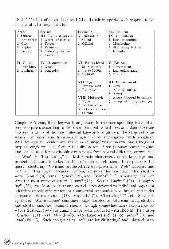
Table ����� List of eleven features IXI and their categories with respect to veaspects of a Bribery situation�
Actor Service Interaction EnvironmentI� O�ce III� Type of service V� Initiator IX� Condition
�� Enterprise �� Obstr� of justice �� Client �� Regular routine�� City �� Favors �� O�cial �� Monitoring�� Region �� Extortion �� Sloppy regulations� Federal � Category change � Irregular
�� Cover�up
II� Client IV� Occurrence VI� Bribe level X� Branch
�� Individual �� Once �� ���K or less �� Government�� Business �� Multiple �� Up to ����K �� Law enforcement
�� �����K �� Other
VII� Type XI� Punishment
�� Infringement �� None�� Extortion �� Administrative
�� ArrestVIII� Network � Arrest followed by release�� None �� Arrest with imprisonment�� Within o�ce�� Between o�ces� Clients
Google or Yahoo� nds keywords or phrases in the corresponding texts� clusters web pages according to the keywords used as features� and then describesclusters in terms of the most relevant keywords or phrases� Two top web siteswhich have been found from searching for �clustering engines� with Google on�� June ���� in London are Vivisimo at hhtp���vivisimo�com and iBoogie athttp���iboogie�tv� The former is built on top of ten popular search enginesand can be used for partitioning web pages from several di erent sources suchas �Web� or �Top stories�� the latter maintains several dozen languages andpresents a hierarchical classication of selected web pages� In response to thequery �clustering� Vivisimo produced ��� web pages in a �Web� category and��� in a �Top news� category� Among top news the most populated clusterswere �Linux� ��� items�� �Stars� ����� and �Bombs� ����� Among general websites the most numerous were �Linux� ����� �Search� Engine� ����� �Computing� ����� etc� More or less random web sites devoted to individual papers orscientists or scientic centers or commercial companies have been listed undercategories �Visualization� ����� �Methods� ���� �Clustering� ���� etc� Such categories as �White papers� contained pages devoted to both computing clustersand cluster analysis� Similar results� though somewhat more favourable towards clustering as data mining� have been produced with iBoogie� Its cluster�Cluster� ���� was further divided into categories such as �computer� ���� and�analysis� ���� Such categories as �software for clustering� and �data cluster
���� EXEMPLARY PROBLEMS ��
ing� have been presented too to refer to a random mix of �� and �� web sitesrespectively�
The activity of generalization so far mainly relies on human experts whosupply understanding of a substantive area behind the text corpus� Humanexperts develop a texttofeature data table that can be further utilized forgeneralization� Such is a collection of �� articles on Bribery cases from central Russian newspapers �������� presented in Table ���� according to �����The features re�ect the following vefold structure of bribery situations� twointeracting sides the o�ce and the client� their interaction� the corrupt servicerendered� and the environment in which it all occurs�
These structural aspects can be characterized by eleven features that canbe recovered from the newspaper articles� they are presented in Table �����
To show how these features can be applied to a newspaper article� let usquote an article that appeared in a newspaper called �Kommersant� on ��March ���� �translated from Russian��
Mayor of a coal town under arrestThursday this week� Mr Evgeny Parshukov� Mayor of town Belovo nearKemerovo� was arrested under a warrant issued by the region attorney� Mr�Valentin Simuchenkov� The mayor is accused of receiving a bribe and abusing his powers for wrongdoing� Before having been elected to the mayoralpost in June ����� he received a credit of ������ roubles from Belovo Division of KUZBASS Transport Bank to support his election campaign� TheBank then cleared up both the money and interest on it� allegedly becauseafter his election Mr� Parshukov ordered the Finance Department of thetown administration� as well as all municipal organisations in Belovo� tomove their accounts into the Transport Bank� Also� the attorney o�ceclaims that in ���� Mr� Parshukov misspent ������� roubles from the townbudget� The money came from the Ministry of Energy specically aimedat creating new jobs for mine workers made redundant because their mineswere getting closed� However� Mr� Parshukov ordered to lend the moneyat a high interest rate to the Municipal Transport agency� Mr� Parshukovdoesn�t deny the facts� He claims however that his actions involve no crime�
A possible coding of the eleven features in this case constitutes the contentsof row �� in Table ����� The table presents �� cases that could be more or lessunambiguously coded �from the original �� cases ������
The prime problem here is similar to those in the Market towns and Digitsdata� to see if there are any patterns at all� To generalize� one has to makesense of patterns in terms of the features� In other words� we are interested ingetting a synoptic description of the data in terms of clusters which are to befound and described�
On the rst glance� no structure exists in the data� Nor could the scientists
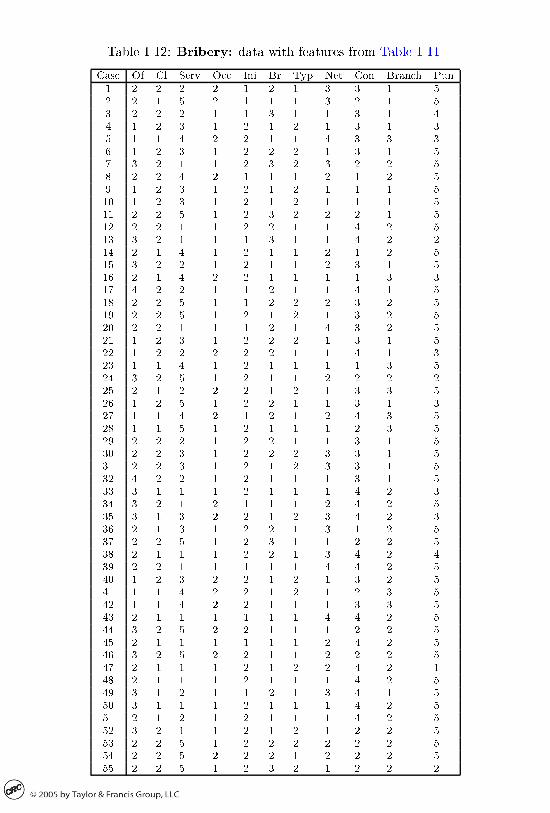
�� WHAT IS CLUSTERING
Table ����� Bribery� data with features from Table �����
Case Of Cl Serv Occ Ini Br Typ Net Con Branch Pun� � � � � � � � � � � �� � � � � � � � � � � �� � � � � � � � � � � � � � � � � � � � � �� � � � � � � � � �� � � � � � � � � � � �� � � � � � � � � � � �� � � � � � � � � � � � � � � � � � � � � ��� � � � � � � � � � � ��� � � � � � � � � � � ��� � � � � � � � � � ��� � � � � � � � � � �� � � � � � � � � � ��� � � � � � � � � � � ��� � � � � � � � � � ��� � � � � � � � � ��� � � � � � � � � � � �� � � � � � � � � � � ��� � � � � � � � � � ��� � � � � � � � � � � ��� � � � � � � � � � ��� � � � � � � � � � �� � � � � � � � � � � ��� � � � � � � � � � � ��� � � � � � � � � � � ��� � � � � � � � � ��� � � � � � � � � � � �� � � � � � � � � � � ��� � � � � � � � � � � ��� � � � � � � � � � � ��� � � � � � � � � � ��� � � � � � � � � � �� � � � � � � � � � ��� � � � � � � � � � ��� � � � � � � � � � � ��� � � � � � � � � � � ��� � � � � � � � � � � � � � � � � � � �� � � � � � � � � � � �� � � � � � � � � � �� � � � � � � � � � �� � � � � � � � � � � � � � � � � � � � �� � � � � � � � � � �� � � � � � � � � � � �� � � � � � � � � � �� � � � � � � � � � � � � � � � � � � � ��� � � � � � � � � � ��� � � � � � � � � � ��� � � � � � � � � � � ��� � � � � � � � � � � �� � � � � � � � � � � ��� � � � � � � � � � � �
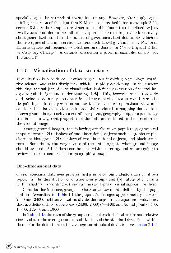
���� EXEMPLARY PROBLEMS ��
specializing in the research of corruption see any� However� after applying anintelligent version of the algorithm KMeans as described later in example �����section ���� a rather simple core structure could be found that is dened by justtwo features and determines all other aspects� The results provide for a reallyshort generalization� �It is the branch of government that determines which ofthe ve types of corrupt services are rendered� Local government � Favors orExtortion� Law enforcement � Obstruction of Justice or CoverUp� and Other� Category Change�� A detailed discussion is given in examples on pp� ������ and ����
����� Visualization of data structure
Visualization is considered a rather vague area involving psychology� cognitive sciences and other disciplines� which is rapidly developing� In the currentthinking� the subject of data visualization is dened as creation of mental images to gain insight and understanding ������ This� however� seems too wideand includes too many nonoperational images such as realistic and surrealistic paintings� In our presentation� we take on a more operational view andconsider that data visualization is an activity related to mapping data onto aknown ground image such as a coordinate plane� geography map� or a genealogytree in such a way that properties of the data are re�ected in the structure ofthe ground image�
Among ground images� the following are the most popular� geographicalmaps� networks� �D displays of onedimensional objects such as graphs or piecharts or histograms� �D displays of twodimensional objects� and block structures� Sometimes� the very nature of the data suggests what ground imageshould be used� All of these can be used with clustering� and we are going toreview most of them except for geographical maps�
One�dimensional data
Onedimensional data over prespecied groups or found clusters can be of twotypes� �a� the distribution of entities over groups and �b� values of a featurewithin clusters� Accordingly� there can be two types of visual support for these�
Consider� for instance� groups of the Market town data dened by the population� According to Table ��� the population ranges approximately between���� and ����� habitants� Let us divide the range in ve equal intervals� bins�that are dened thus to have size ������������������ and bound points ����������� ������ and ������
In Table ���� the data of the groups are displayed� their absolute and relativesizes and also the average numbers of Banks and the standard deviations withinthem� For the denitions of the average and standard deviation see section ������

�� WHAT IS CLUSTERING
I II III IV V (a)
25
11
42
V IV
III I
II
(b)
Figure ���� Histogram �a and pie�chart �b presenting the distribution of Populationover �ve equally sized bins in Market data�
Figure ��� shows two traditional displays for the distribution� a histogram�part �a� on the left� in which bars are proportional to the group sizes and apie�chart in which a pie is partitioned into slices proportional to the cluster sizes�part �b� on the right�� These two point to di erent features of the distribution�The histogram positions the categories along the horizontal axis� thus providingfor a possibility to see the distribution�s shape� which can be quite useful whenthe categories have been created as interval bins of a quantitative feature� asis this case� The piechart points to the fact that the group sizes sum up tothe total so that one can see what portions of the pie account for di erentcategories�
One�dimensional data within groups
To visualize a quantitative feature within prespecied groups� box�plots andstick�plots are utilized� They show withincluster central values and their dis
Table ����� Population groups� Data of the distribution of population groupsand numbers of banks within them�
Group Size Frequency � Banks Std Banks
I �� ���� ��� ����II �� ���� ���� ����III � ��� �� ��IV � ��� ��� ����V � ��� ���� ����
Total �� � ���� ����
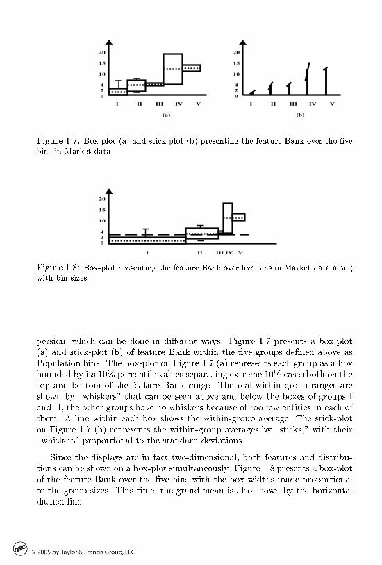
���� EXEMPLARY PROBLEMS ��
20
15
10
4 2 0
20
15
10
4 2 0
I II III IV V
(a)
I II III IV V
(b)
Figure ���� Box�plot �a and stick�plot �b presenting the feature Bank over the �vebins in Market data�
20
15
10
4 2 0
I II III IV V
Figure ���� Box�plot presenting the feature Bank over �ve bins in Market data alongwith bin sizes�
persion� which can be done in di erent ways� Figure ��� presents a boxplot�a� and stickplot �b� of feature Bank within the ve groups dened above asPopulation bins� The boxplot on Figure ��� �a� represents each group as a boxbounded by its �� percentile values separating extreme �� cases both on thetop and bottom of the feature Bank range� The real within group ranges areshown by �whiskers� that can be seen above and below the boxes of groups Iand II� the other groups have no whiskers because of too few entities in each ofthem� A line within each box shows the withingroup average� The stickploton Figure ��� �b� represents the withingroup averages by �sticks�� with their�whiskers� proportional to the standard deviations�
Since the displays are in fact twodimensional� both features and distributions can be shown on a boxplot simultaneously� Figure ��� presents a boxplotof the feature Bank over the ve bins with the box widths made proportionalto the group sizes� This time� the grand mean is also shown by the horizontaldashed line�
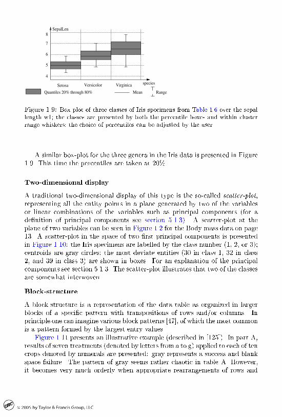
�� WHAT IS CLUSTERING
4
5
6
7
8
Setosa Versicolor Virginica species
SepalLen
Quantiles 20% through 80% Mean Range
Figure ���� Box�plot of three classes of Iris specimens from Table ��� over the sepallength w�� the classes are presented by both the percentile boxes and within clusterrange whiskers� the choice of percentiles can be adjusted by the user�
A similar boxplot for the three genera in the Iris data is presented in Figure���� This time the percentiles are taken at �� �
Two�dimensional display
A traditional twodimensional display of this type is the socalled scatter�plot�representing all the entity points in a plane generated by two of the variablesor linear combinations of the variables such as principal components �for adenition of principal components see section ������� A scatterplot at theplane of two variables can be seen in Figure ��� for the Body mass data on page��� A scatterplot in the space of two rst principal components is presentedin Figure ����� the Iris specimens are labelled by the class number ��� �� or ���centroids are gray circles� the most deviate entities ��� in class �� �� in class�� and �� in class �� are shown in boxes� For an explanation of the principalcomponents see section ������ The scatterplot illustrates that two of the classesare somewhat interwoven�
Block�structure
A blockstructure is a representation of the data table as organized in largerblocks of a specic pattern with transpositions of rows and�or columns� Inprinciple one can imagine various block patterns ����� of which the most commonis a pattern formed by the largest entry values�Figure ���� presents an illustrative example �described in ������� In part A�
results of seven treatments �denoted by letters from a to g� applied to each of tencrops denoted by numerals are presented� gray represents a success and blankspace failure� The pattern of gray seems rather chaotic in table A� However�it becomes very much orderly when appropriate rearrangements of rows and
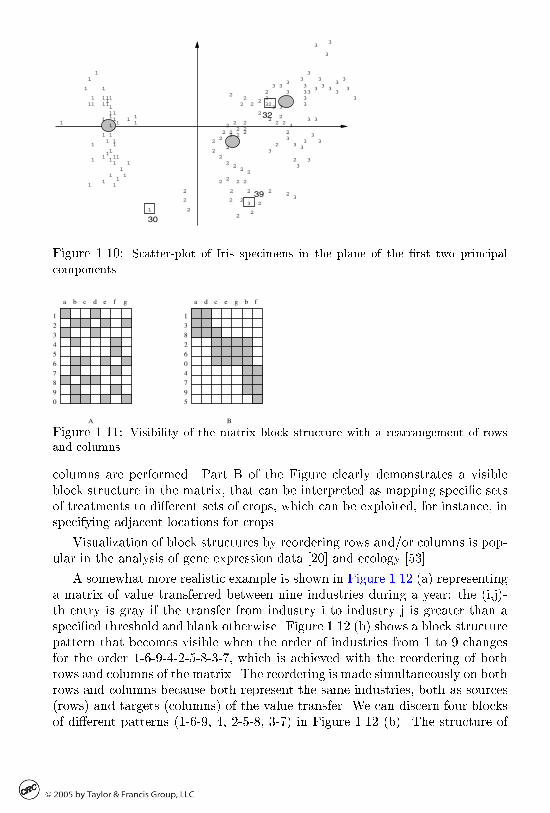
���� EXEMPLARY PROBLEMS ��
1 11
1 111
11 1 11 1111
111 1
1
1 11 111 1
1
1
111111
1
1
1 1
1
11
1
1
1
1
1
22 2
2 22 222
2 2 22
222 2
2 2
2222
2 2
2 2
2
3 2
22
2
2 2 2
2
2
2
22
2
22
22 2
22
2
2
3
3
3
33 3
3
3
333
3 3
3 333
3 33
3
3333333
3
33 3
3
33
3
3
3
33
30
39
32
Figure ����� Scatter�plot of Iris specimens in the plane of the �rst two principal
components�
1
2
3
4
5
6
7
8
9
0
1
3
8
2
6
0
4
7
9
5
a b c d e f g a d c e g b f
A B
Figure ����� Visibility of the matrix block structure with a rearrangement of rowsand columns�
columns are performed� Part B of the Figure clearly demonstrates a visibleblock structure in the matrix� that can be interpreted as mapping specic setsof treatments to di erent sets of crops� which can be exploited� for instance� inspecifying adjacent locations for crops�
Visualization of block structures by reordering rows and�or columns is popular in the analysis of gene expression data ���� and ecology �����
A somewhat more realistic example is shown in Figure ���� �a� representinga matrix of value transferred between nine industries during a year� the �i�j�th entry is gray if the transfer from industry i to industry j is greater than aspecied threshold and blank otherwise� Figure ���� �b� shows a block structurepattern that becomes visible when the order of industries from � to � changesfor the order ���������� which is achieved with the reordering of bothrows and columns of the matrix� The reordering is made simultaneously on bothrows and columns because both represent the same industries� both as sources�rows� and targets �columns� of the value transfer� We can discern four blocksof di erent patterns ����� �� ���� ��� in Figure ���� �b�� The structure of
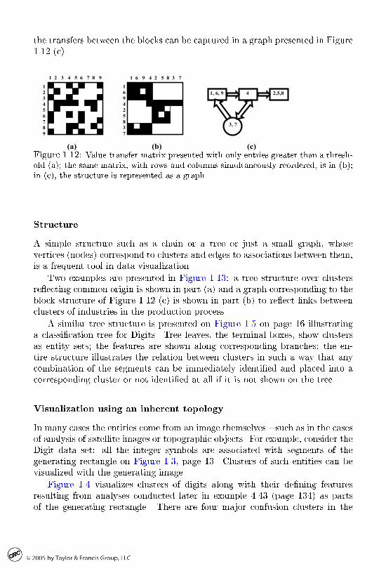
�� WHAT IS CLUSTERING
the transfers between the blocks can be captured in a graph presented in Figure���� �c��
123456789
169425837
1 2 3 4 5 6 7 8 9 1 6 9 4 2 5 8 3 7
1, 6, 9 4 2,5,8
3, 7
(a) (b) (c) Figure ����� Value transfer matrix presented with only entries greater than a thresh�old �a � the same matrix with rows and columns simultaneously reordered is in �b �in �c the structure is represented as a graph�
Structure
A simple structure such as a chain or a tree or just a small graph� whosevertices �nodes� correspond to clusters and edges to associations between them�is a frequent tool in data visualization�
Two examples are presented in Figure ����� a tree structure over clustersre�ecting common origin is shown in part �a� and a graph corresponding to theblock structure of Figure ���� �c� is shown in part �b� to re�ect links betweenclusters of industries in the production process�
A similar tree structure is presented on Figure ��� on page �� illustratinga classication tree for Digits� Tree leaves� the terminal boxes� show clustersas entity sets� the features are shown along corresponding branches� the entire structure illustrates the relation between clusters in such a way that anycombination of the segments can be immediately identied and placed into acorresponding cluster or not identied at all if it is not shown on the tree�
Visualization using an inherent topology
In many cases the entities come from an image themselves � such as in the casesof analysis of satellite images or topographic objects� For example� consider theDigit data set� all the integer symbols are associated with segments of thegenerating rectangle on Figure ���� page ��� Clusters of such entities can bevisualized with the generating image�
Figure ��� visualizes clusters of digits along with their dening featuresresulting from analyses conducted later in example ���� �page ���� as partsof the generating rectangle� There are four major confusion clusters in the
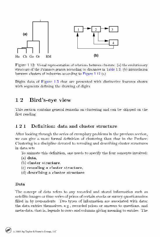
���� BIRD�S�EYE VIEW ��
1 2 3
4
Hu Ch Go Or RM
(a)
(b)
Figure ����� Visual representation of relations between clusters� �a the evolutionarystructure of the Primates genera according to distances in Table ���� �b interrelationbetween clusters of industries according to Figure ���� �c �
Digits data of Figure ��� that are presented with distinctive features shownwith segments dening the drawing of digits�
��� Bird�s�eye view
This section contains general remarks on clustering and can be skipped on therst reading�
����� De�nition� data and cluster structure
After looking through the series of exemplary problems in the previous section�we can give a more formal denition of clustering than that in the Preface�Clustering is a discipline devoted to revealing and describing cluster structuresin data sets�
To animate this denition� one needs to specify the four concepts involved�
�a� data�
�b� cluster structure�
�c� revealing a cluster structure�
�d� describing a cluster structure�
Data
The concept of data refers to any recorded and stored information such assatellite images or time series of prices of certain stocks or survey questionnaireslled in by respondents� Two types of information are associated with data�the data entries themselves� e�g�� recorded prices or answers to questions� andmetadata� that is� legends to rows and columns giving meaning to entries� The
�� WHAT IS CLUSTERING
aspect of developing and maintaining databases of records� taking into accountthe relations stored in metadata� is very important for data mining ���� ��� ����In this text� for the sake of linearity of presentation� we concentrate on a
generic data format only� the socalled entitytovariable table whose entriesrepresent values of prespecied variables at prespecied entities�The variables are synonymously called attributes� features� characteristics�
characters and parameters� Such words as case� object� observation� instance�record are in use as synonyms to the term� entity� accepted here�The data table format of data often arises directly from experiments or
observations� from surveys� and from industrial or governmental statistics� Thisalso is a conventional form for presenting database records� Other data typessuch as signals or images can be modelled in this format� too� via digitalizedrepresentation� However� a digital representation� typically� involves much moreinformation than can be kept in a data table format� Especially important isthe spatial arrangement of pixels� which is not� typically� maintained in theconcept of data table� The contents of a data table are assumed to be invariantunder permutations of rows and columns and corresponding metadata�Another data type traditionally considered in clustering is the similarity
or dissimilarity between entities �or features�� The concept of similarity ismost important in clustering� similar objects are to be put into the same cluster and dissimilar into di erent clusters� There have been invented dozens of�dis�similarity indices� Some of them nicely t into theoretical frameworks andwill be considered further in the text�One more data type considered in this text is cooccurrence or �ow tables
that represent the same substance distributed between di erent categories suchas Confusion data in Table ��� in which the substance is the scores of individuals�An important property of this type of data is that any part of the data table�referred to a subset of rows and �or a subset of columns� can be meaningfullyaggregated by summing the part of the total �ow within the subset of rows�and�or the subset of columns�� The sums represent the total �ow to� from�and within the subset�s�� Thus� problems of clustering and aggregating arenaturally linked here� Until recently� this type of data appeared as a result ofdata analysis rather than input to it� Currently it has become one of the majordata formats� Examples are� distributions of households purchasing variouscommodities or services across postal districts or other regional units� countsof telephone calls across areas� and counts of visits in various categories ofwebsites�
Cluster structure
The concept of cluster typically refers to a set of entities that is cohesive insuch a way that entities within are more similar to each other than to the outerentities�
���� BIRD�S�EYE VIEW ��
Three major types of cluster structures are� �a� a single cluster consideredagainst the rest or whole of the data� �b� a partition of the entity set in a setof clusters� and �c� a �nested� hierarchy of clusters�
Of these three� partition is the most conventional� probably because it isrelevant to both science and management� the major forces behind scienticdevelopments� A scientist� as well as a manager� wants unequivocal controlover the entire universe under consideration� This is why they may wish topartition the entity set into a set of nonoverlapping clusters�
In some situations there is no need for total clustering� The user may bequite satised with getting just a single �or few� cluster�s� and leaving the restcompletely unclustered� Examples�
��� a bank manager wants to learn how to discern potential fraudsters fromother clients or
��� a marketing researcher separates a segment of customers prone to purchase a particular product or
��� a bioinformatician seeks a set of proteins homologous to a query proteinsequence�
Incomplete clustering is a recently recognized addition to the body of clusteringapproaches� very suitable not only at the situations above but also as a toolfor conventional partitioning via clusterbycluster procedures such as thosedescribed in section ����
The hierarchy is the oldest and probably least understood of the clusterstructures� To see how important it is� it should su�ce to recall that the Aristotelian approach to classication encapsulated in library classications andbiological taxonomies is always based on hierarchies� Moreover� hierarchy underlies most advanced data processing tools such as wavelets and quadtrees� Itis ironic then that as a cluster structure in its own right� the concept of hierarchy rarely features in clustering� especially when clustering is conned to thecohesive partitioning of geometric points�
����� Criteria for revealing a cluster structure
To reveal a cluster structure in a data table means to nd such clusters thatallow the individual characteristics of entities to be substituted by aggregatecharacteristics of clusters� A cluster structure is revealed by a method according to a criterion of how well the data are represented by clusters� Criteriaand methods are� to an extent� independent from each other so that the samemethod such as agglomeration or splitting can be used with di erent criteria�
Criteria usually are formulated in terms of �dis�similarity between entities�This helps in formalizing the major idea that entities within clusters should besimilar to each other and those between clusters dissimilar� Dozens of similaritybased criteria developed so far can be categorized in three broad classes�

�� WHAT IS CLUSTERING
��� Denitionbased�
��� Indexbased� and
��� Computationbased�
The rst category comprises methods for nding clusters according to anexplicit denition of a cluster� An example� A cluster is a subset S of entitiessuch that for all i� j in S the similarity between i and j is greater than thesimilarities between these and any k outside S� Such a property must hold forall entities with no exceptions� which means that well isolated clusters are ratherrare in real world data� However� when the denition of cluster is relaxed toinclude less isolated clusters� too many may then appear� This is why denitionbased methods are not popular in practical clustering�
A criterion in the next category involves an index� that is� a numericalfunction that scores di erent cluster structures and� in this way� may guide theprocess of choosing the best� However� not all indices are suitable for obtainingreasonable clusters� Those derived from certain modelbased considerationstend to be computationally hard to optimize� Optimizing methods are thusbound to be local and� therefore� heavily reliant on the initial settings� whichinvolve� in the case of KMeans clustering� prespecifying the number of clustersand the location of their central points� Accordingly� the found cluster structuremay be rather far from the global optimum and� thus� must be validated� Clustervalidation may be done according to internal criteria such as that involved inthe optimization process or external criteria comparing the clusters found withthose known from external considerations or according to its stability withrespect to randomly resampling entities�features� These will be outlined insection ��� and exemplied in section ������
The third category comprises computation methods involving various heuristics for individual entities to be added to or removed from clusters� for mergingor splitting clusters� and so on� Since operations of this type are necessarily local� they resemble local search optimization algorithms� though� typically� haveno unique guiding scoring index to follow� thus� can include various tricks making them �exible� However� such �exibility is associated with an increase in thenumber of ad hoc parameters such as various similarity thresholds and� in thisway� turning clustering from a reproducible activity into a kind of magic� Validation of a cluster structure found with a heuristicbased algorithm becomes anecessity�
In this book� we adhere to an indexbased principle� which scores a clusterstructure against the data from which it has been built� The cluster structurehere is used as a device for reconstructing the original data table� the closerthe reconstructed data are to the original ones� the better the structure� Itis this principle that is called the data recovery approach in this book� Manyindexbased and computationbased clustering methods can be reinterpretedaccording to the principle� which allows us to see interrelations between dif
���� BIRD�S�EYE VIEW ��
ferent methods and concepts for revealing and analyzing clustering structures�New methods can be derived from the principle too �see Chapter �� especiallysections �������� It should be noted� though� that we will use only the moststraightforward rules for reconstructing the data from cluster structures�
����� Three types of cluster description
Cluster descriptions help in understanding� explaining and predicting clusters� These may come in di erent formats of which the most popular are thefollowing three� �a� Representative� �b� Tendency� �c� Conceptual description�
A representative� or a prototype� is an object such as a literary character ora sort of wine or mineral� representing the most typical features of a cluster�This format is useful in giving a meaning to entities that are easily availableempirically but di�cult to conceptually describe� There is evidence that someaggregate language constructs� such as �fruit�� are mentally maintained viaprototypes� such as �apple� ����� In clustering� the representative is usually themost central entity in a cluster�
A tendency expresses a cluster�s most likely features such as its way ofbehavior or pattern� It is usually related to the center of gravity of the clusterand its di erences from the average� In this respect� the tendency models theconcept of type in classication studies�
A conceptual description may come in the form of a classication tree builtfor predicting a class or partition� Another form of conceptual description is anassociation� or production� rule� stating that if an object belongs to a clusterthen it must have such and such features� Or� vice versa� if an object satisesthe premise� then it belongs in the cluster� The simplest conceptual descriptionof a cluster is a statement of the form �the cluster is characterized by the featureA being between values a� and a��� The existence of a feature A� which aloneis su�cient to distinctively describe a cluster is a rare occurrence of luck in datamining� Typically� features in data are rather supercial and do not expressessential properties of entities and thus cannot be the basis of straightforwarddescriptions�
The subject of cluster description overlaps that of supervised machine learning and pattern recognition� Indeed� given a cluster� having its description mayallow one to predict� for new objects� whether they belong to the cluster ornot� depending on how much they satisfy the description� On the other hand�a decision rule obtained with a machine learning procedure� especially� for example� a classsication tree� can be considered a cluster description usable forthe interpretation purposes� Still the goals are di erent� interpretation in clustering and prediction in machine learning� However� cluster description is asimportant in clustering as cluster nding�
�� WHAT IS CLUSTERING
����� Stages of a clustering application
Typically� clustering as a data mining activity involves the following ve stages�
A� Developing a data set�
B� Data preprocessing and standardizing�
C� Finding clusters in data�
D� Interpretation of clusters�
E� Drawing conclusions�
To develop a data set one needs to dene a substantive problem or issue�however vague it may be� and then determine what data set related to the issuecan be collected from an existing database or set of experiments or survey� etc�Data preprocessing is the stage of preparing data processing by a cluster
ing algorithm� typically� it includes developing a uniform data set� frequentlycalled a ��at� le� from a database� checking for missing and unreliable entries�rescaling and standardizing variables� deriving a unied similarity measure� etc�
The cluster nding stage involves application of a clustering algorithm andresults in a �series of� cluster structure�s� to be presented� along with interpretation aids� to substantive specialists for an expert judgement and interpretationin terms of features� both those utilized for clustering �internal features� andthose not utilized �external features�� At this stage� the expert may see no relevance in the results and suggest a modication of the data by adding�removingfeatures and�or entities� The modied data is subject to the same processingprocedure� The nal stage is the drawing of conclusions� with respect to theissue in question� from the interpretation of the results� The more focussed arethe regularities implied by the ndings� the better the quality of conclusions�
There is a commonly held opinion among specialists in data analysis thatthe discipline of clustering concerns only the proper clustering stage C whilethe other four are the concern of specialists in the substance of the particularissue for which clustering is performed� Indeed� typically� clustering results cannot and are not supposed to solve the entire substantive problem� but ratherrelate to an aspect of it�
On the other hand� clustering algorithms are supposedly most applicableto situations and issues in which the user�s knowledge of the domain is moresupercial than profound� What are the choices regarding data preprocessing�initial settings in clustering and interpretation of results � facing the laymenuser who has an embryonic knowledge of the domain� More studies and experiments� In most cases� this is not practical advice� Sometimes a more viablestrategy would be to better utilize properties of the clustering methods at hand�
���� BIRD�S�EYE VIEW ��
At this stage� no modelbased recommendations can be made about theinitial and nal stages� A and E� However� the data recovery approach doesallow us to use the same formalisms for tackling not stage C only� but also Band D� see sections ���� ��� and ��� for related prescriptions and discussions�
����� Clustering and other disciplines
The concepts involved make clustering a multidisciplinary activity on its own�regardless of its many applications� In particular�
�� Data relates to database� data structure� measurement� similarity anddissimilarity� statistics� matrix theory� metric and linear spaces� graphs�data analysis� data mining� etc�
�� Cluster structure relates to discrete mathematics� abstract algebra�cognitive science� graph theory� etc�
�� Revealing cluster structures relates to algorithms� matrix analysis� optimization� computational geometry� etc�
�� Describing clusters relates to machine learning� pattern recognition�mathematical logic� knowledge discovery� etc�
����� Dierent perspectives of clustering
Clustering is a discipline on the intersection of di erent elds and can be viewedfrom di erent angles� which may be sometimes confusing because di erent perspectives may contradict each other� A question such as� �How many clustersare out there��� which is legitimate in one perspective� can be meaninglessin the other� Similarly� the issue of validation of clusters may have di erentsolutions in di erent frameworks� The author nds it useful to distinguish between the perspectives supplied by statistics� machine learning� data miningand classication�
Statistics perspective
Statistics tends to view any data table as a sample from a probability distribution whose properties or parameters are to be estimated with the data� In thecase of clustering� clusters are supposed to be associated with di erent probabilistic distributions which are intermixed in the data and should be recoveredfrom it�Within this approach� such questions as �How many clusters are out there��
and �How to preprocess the data�� are well substantiated and can be dealt withaccording to the assumptions of the underlying model�
�� WHAT IS CLUSTERING
In many cases the statistical paradigm suits quite well and should be appliedas the one corresponding most to what is called the scientic method� makea hypothesis of the phenomenon in question� then look for relevant data andcheck how the hypothesis ts them�
A trouble with this approach is that in most cases clustering is appliedto phenomena of which almost nothing is known� not only of their underlying mechanisms but of the very features measured or to be measured� Thenany modelling assumptions of the data generation would be necessarily ratherarbitrary and so too conclusions based on them�
Moreover in many cases the set of entities is rather unique and cannot beconsidered a sample from a larger population� such as the set of Europeancountries or single malt whisky brands�
Sometimes the very concept of a cluster as a probabilistic distribution seemsto not t into a clustering goal� Look� for example� at a bellshaped Gaussiandistribution which is considered a good approximation for such variables as theheight or weight of young male individuals of the same ethnicity so that theyform a cluster corresponding to the distribution� However� when confrontedwith the practical issue of dividing people� for example� according to theirghting capabilities �such as in military conscription or in the sport of boxing��the set cannot be considered a homogeneous cluster anymore and must befurther partitioned into more homogeneous strata� Some say that there mustbe a boundary between �natural� clusters and clusters to be drawn on purpose�that a bellshape distribution corresponds to a natural cluster and a boxingweight category to an articial one� However� it is not always easy to distinguishwhich situation is which� There will always be situations when a cluster ofpotentially weak ghters �or bad customers� or homologous proteins� must becut out from the rest�
Machine learning perspective
Machine learning tends to view the data as a device for learning how to predictprespecied or newly created categories� The entities are considered as comingone at a time so that the machine can learn adaptively in a supervised manner�To theorize� the �ow of data must be assumed to come from a probabilisticpopulation� an assumption which has much in common with the statistics approach� However� it is prediction rather than model tting which is the centralissue in machine learning�
Such a shift in the perspective has led to the development of strategies forpredicting categories such as decision trees and support vector machines as wellas resampling methods such as the bootstrap and crossvalidation for dealingwith limited data sets�
���� BIRD�S�EYE VIEW ��
Data mining perspective
Data mining is not much interested in re�ection on where the data have comefrom nor how they have been collected� It is assumed that a data set or databasehas been collected already and� however bad or well it re�ects the properties ofthe phenomenon in question� the major concern is in nding patterns and regularities within the data as they are� Machine learning and statistics methodsare welcome here � for their capacity to do the job�
This view� started as early as in the sixties and seventies in many countriesincluding France� Russia and Japan in such subjects as analysis of questionnaires or of interindustrial transfers� was becoming more and more visible�but it did not make it into prominence until the nineties� By that time� bigwarehouse databases became available� which led to the discovery of patternsof transactions with the socalled association search methods� The patternsproved themselves correct when superstores increased prots by accommodating to them�
Data mining is a huge activity on the intersection of databases and dataanalysis methods� Clustering is a recognized part of it� The data recoveryapproach which is maintained in this book obviously ts within data miningvery well� because it is based only on the data available�
It should be added that the change of the paradigm from modeling of mechanisms of data generation to data mining has drastically changed requirementsto methods and programs� According to the statistics approach� the user mustknow the models and methods he uses� if a method is applied wrongly� theresults can be wrong too� Thus� application of statistical methods is limitedwithin a small circle of experts� In data mining� it is the patterns not methodsthat matter� This shifts the focus of computer programs from statistics to theuser�s substantive area and makes them userfriendly�
Similarly� the validation objectives seem to diverge here� in statistics andmachine learning the stress goes on the consistency of the algorithms� which isnot quite so important in data mining� in which it is the consistency of patterns�not algorithms� which matters the most�
Classi�cation knowledge�discovery perspective
The classication perspective is rarely discussed indeed� In data mining theterm �classication� is usually referred to in a very limited sense� as an activityof assigning prespecied categories �classes� to entities� in contrast to clusteringwhich assigns entities with newly created categories �clusters��
According to its genuine meaning� classication is an actual or ideal arrangement of entities under consideration in classes to�
��� shape and keep knowledge�
�� WHAT IS CLUSTERING
��� capture the structure of phenomena� and
��� relate di erent aspects of a phenomenon in question to each other�
These make the concept of classication a specic mechanism for knowledge discovery and maintenance� Consider� for instance� the Periodic Chartof chemical elements� Its rows correspond to numbers of electron shells in theatoms� and its columns to the numbers of electrons in the external shell thuscapturing the structure of the phenomenon� These also relate to most important physical properties and chemical activities of the elements thus associatingdi erent aspects of the phenomenon� And this is a compact form of representing the knowledge� moreover� historically it is this form itself� developed ratherempirically� that made possible rather fast progress to the current theories ofthe matter�In spite of the fact that the notion of classication as part of scientic
knowledge was introduced by the ancient Greeks �Aristotle and the like� thevery term �classication� seems a missing item in the vocabulary of currentscientic discourse� This may have happened because in traditional sciences�classications are dened within well developed substantive theories accordingto variables which are dened as such within the theories� Thus� there has beenno need in specic theories for classication�Clustering should be considered as classication based on empirical data
in a situation when clear theoretical concepts and denitions are absent andthe regularities are unknown� Thus� the clustering goals should relate to theclassication goals above� This brings one more aspect to clustering� Consider�for example� how one can judge whether a clustering is good or bad� Accordingto the classication�knowledgediscovery view� this is easy and has nothingto do with statistics� just look at how well clusters t within the existingknowledge� how well they allow updating� correcting and extending�Somewhat simplistically� one might say that two of the points stressed in
this book� that of the data recovery approach and the need to not only nd�but describe clusters� t well into the two perspectives� the former into datamining and the latter into classication as knowledge discovery�
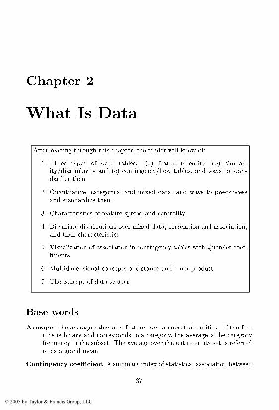
Chapter �
What Is Data
After reading through this chapter� the reader will know of�
�� Three types of data tables� �a� featuretoentity� �b� similarity�dissimilarity and �c� contingency��ow tables� and ways to standardize them�
�� Quantitative� categorical and mixed data� and ways to preprocessand standardize them�
�� Characteristics of feature spread and centrality�
�� Bivariate distributions over mixed data� correlation and association�and their characteristics�
�� Visualization of association in contingency tables with Quetelet coefcients�
�� Multidimensional concepts of distance and inner product�
�� The concept of data scatter�
Base words
Average The average value of a feature over a subset of entities� If the feature is binary and corresponds to a category� the average is the categoryfrequency in the subset� The average over the entire entity set is referredto as a grand mean�
Contingency coe�cient A summary index of statistical association between
��
© 2005 by Taylor & Francis Group, LLC
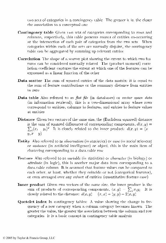
�� WHAT IS DATA
two sets of categories in a contingency table� The greater it is� the closerthe association to a conceptual one�
Contingency table Given two sets of categories corresponding to rows andcolumns� respectively� this table presents counts of entities cooccurringat the intersection of each pair of categories from the two sets� Whencategories within each of the sets are mutually disjoint� the contingencytable can be aggregated by summing up relevant entries�
Correlation The shape of a scatterplot showing the extent to which two features can be considered mutually related� The �productmoment� correlation coe�cient captures the extent at which one of the features can beexpressed as a linear function of the other�
Data scatter The sum of squared entries of the data matrix� it is equal tothe sum of feature contributions or the summary distance from entitiesto zero�
Data table Also referred to as �at �le �in databases� or vector space data�in information retrieval�� this is a twodimensional array whose rowscorrespond to entities� columns to features� and entries to feature valuesat entities�
Distance Given two vectors of the same size� the �Euclidean squared� distanceis the sum of squared di erences of corresponding components� d�x� y� �P
i�xi � yi��� It is closely related to the inner product� d�x� y� � �x �
y� x� y��
Entity Also referred to as observation �in statistics� or case �in social sciences�or instance �in articial intelligence� or object� this is the main item ofclustering corresponding to a data table row�
Feature Also referred to as variable �in statistics� or character �in biology� orattribute �in logic�� this is another major data item corresponding to adata table column� It is assumed that feature values can be compared toeach other� at least� whether they coincide or not �categorical features��or even averaged over any subset of entities �quantitative feature case��
Inner product Given two vectors of the same size� the inner product is thesum of products of corresponding components� �x� y� �
Pi xiyi� It is
closely related to the distance� d�x� y� � �x� x� ! �y� y�� ��x� y��Quetelet index In contingency tables� A value showing the change in fre
quency of a row category when a column category becomes known� Thegreater the value� the greater the association between the column and rowcategories� It is a basic concept in contingency table analysis�
© 2005 by Taylor & Francis Group, LLC
BASE WORDS ��
Range The interval in which a feature takes its values� the di erence betweenthe feature maximum and minimum over a data set�
Scatter plot A graph presenting entities as points on the plane formed by twoquantitative features�
Variance The average of squared deviations of feature values from the average�
© 2005 by Taylor & Francis Group, LLC

�� WHAT IS DATA
��� Feature characteristics
����� Feature scale types
The Masterpieces data in Table ���� will be used to illustrate data handlingconcepts in this section� For the reader�s convenience� the table is reprintedhere as Table ����A data table of this type represents a unity of the set of rows� always denoted
as I further on� the set of columns denoted by V and the table contents X � theset of values xiv in rows i � I and columns v � V � The number of rows� orcardinality of I � jI j� will be denoted by N � and the number of columns� thecardinality of V � jV j� by M � Rows will always correspond to entities� columnsto features� Whatever metadata of entities may be known� are all to be putas the features� except for names� that may be maintained as a list associatedwith I � As to the features v � V � it is assumed that each has a measurementscale assigned to it� and of course a name�All withincolumn entries are supposed to have been measured in the same
scale and thus comparable within the scale� this is not so over rows in Y � Threedi erent types of scales that are present in Table ��� and will be dealt within the remainder are quantitative �LenSent� LenDial� and NChar�� nominal�Narrative� and binary �SCon�� Let us elaborate on these scale types�
Table ���� Masterpieces� Masterpieces of ��th century� the �rst three by CharlesDickens ��������� the next three by Mark Twain ��������� and the last two byLeo Tolstoy ��������� �
Title LenSent LenDial NChar SCon Narrative
Oliver Twist ��� ���� � No ObjectiveDombey and Son ���� ��� � No ObjectiveGreat Expectations ���� ��� � No Personal
Tom Sawyer ���� ���� � Yes ObjectiveHuckleberry Finn ���� ���� � Yes PersonalYankee at King Arthur ���� ���� � Yes Personal
War and Peace ���� ��� � Yes DirectAnna Karenina ���� ��� � Yes Direct
�� Quantitative� A feature is quantitative if the operation of taking itsaverage is meaningful�
It is quite meaningful to compare the average values of feature LenS orLenD for di erent authors in Table ���� Somewhat less convincing is thecase of NumC which must be an integer� some authors even consider such
© 2005 by Taylor & Francis Group, LLC
���� FEATURE CHARACTERISTICS ��
�counting� features a di erent scale type� Still� we can safely say thaton average Tolstoy�s novels have larger numbers of principal charactersthan those by Dickens or Twain� This is why counting features are alsoconsidered quantitative in this text�
�� Nominal� A categorical feature is said to be nominal if its categories are�i� disjoint� that is� no entity can fall in more than one of them� and �ii�not ordered� that is� they only can be compared with respect to whetherthey coincide or not� Narrative� in Table ���� is such a feature�
Categorical features maintaining �ii� but not �i� are referred to as multichoice variables� For instance� Masterpieces data might include a featurethat presents a list of social themes raised in a novel� which may containmore than one element� That would produce a onetomany mapping ofthe entities to the categories� that is� social themes� There is no problemin treating this type of data within the framework described here� Forinstance� the Digit data table may be treated as that representing the only�multichoice� variable �Segment� which has the set of seven segments asits categories�
Categorical features that maintain �i� but have their categories orderedare called rank variables� Variable Bribe level in the Bribery data ofTables ���� and ���� is rank� its three categories are obviously orderedaccording to the bribe size� Traditionally� it is assumed for the rankvariables that only the order of categories matters and intervals betweenthem are irrelevant� That is� rank categories may accept any quantitativecoding which is compatible with their ordering� This makes rank featuresdi�cult to deal with in the context of mixed data tables� We maintaina di erent view� going back to C� Spearman� the ranks are treated asnumerical values and the rank variables are considered thus quantitativeand processed accordingly� In particular� seven of the eleven variablesin Bribery data �II� Client� IV� Occurrence� V� Initiator� VI� Bribe� VII�Type� VIII� Network� and XI� Punishment� will be considered ranked withranks assigned in Table ���� and treated as quantitative values�
There are two approaches to the issue of involving qualitative featuresinto analysis� According to one� more traditional� approach� categoricalvariables are considered nontreatable quantitatively� The only quantitative operation admitted for categories is counting the number or frequencyof its occurrences at various subsets� To conduct cluster analysis� categorical data� according to this view� can only be utilized for deriving anentitytoentity �dis�similarity measure� Then this measure can be usedfor nding clusters�
A di erent approach is maintained and further developed here� a categorydenes a quantitative zeroone variable on entities� with one corresponding
© 2005 by Taylor & Francis Group, LLC
�� WHAT IS DATA
to its presence and zero absence� which is treated then as such� We willsee later that this view� in fact� does not contradict the former one butrather ts into it with geometrically and statistically sound specications�
�� Binary� A qualitative feature is said to be binary if it has two categorieswhich can be thought of as Yes or No answer to a question such as feature SCon in Table ���� A twocategory feature can be considered eithera nominal or binary one� depending on the context� For instance� feature�Gender� of a human should be considered a nominal feature� whereasthe question �Are you female�� a binary feature� because the latter assumes that it is the �female�� not �male�� category which is of interest�Operationally� the di erence between these two types will amount to howmany binary features should be introduced to represent the feature under consideration in full� Feature �Gender� cannot be represented by onecolumn with Yes or No categories� two are needed� one for �Female� andone for �Male��
����� Quantitative case
As mentioned� we consider that the meaningfulness of taking the average is adening property of a quantitative variable� Given a feature v � V whose valuesyiv � i � I � constitute a column in the data table� its average over entity subsetS � I is dened by the formula
cv�S� � ���NS�Xi�S
yiv �����
where NS is the number of entities in S�
The average cv � cv�I� of v � V over the entire set I is sometimes referredto as grand mean� After grand mean cv of v � V has been subtracted from allelements of the columnfeature v � V � the grand mean of v becomes zero� Sucha variable is referred to as centered�
It should be mentioned that usually the quantitative scale is dened somewhat di erently� not in terms of the average but the socalled admissible transformations y � ��x�� The scale type is claimed to depend on the set of transformations � which are considered admissible� that is� do not change the scalecontents� For the quantitative feature scales� those that are admissible aretransformations such as y � ax ! b converting all x values into y values bychanging the scale factor a times and shifting the scale origin at b� Transformations y � ��x� of this type� with ��x� � ax!b for some real a and b� are referredto as a�ne transformations� For instance� the temperature Celsius scale x istransformed into the temperature Fahrenheit scale with ��x� � ���x!��� Stan
© 2005 by Taylor & Francis Group, LLC
���� FEATURE CHARACTERISTICS ��
dardizations of data with a�ne transformations are at the heart of our approachto clustering�Our denition is compatible with the one given above� Indeed� if a feature
x admits a�ne transformations� it is meaningful to compare its average valuesover various entity sets� Let xJ and xK be the averages of sets fxj � j � Jg andfxk � k � Kg respectively� and� say� xJ � xK � Does the same automaticallyhold for the averages of y � ax! b over J and K� To answer this question� weconsider values yj � axj!b� j � J � and yk � axk!b� k � K and calculate theiraverages� yJ and yK � It is easy to prove that yK � axK ! b and yJ � axJ ! bso that any relation between xJ and xK remains the same for yJ and yK � upto the obvious reversal when a is negative �which means that rescaling involveschange of the direction of the scale��Other indices of �centrality� have been considered too� the most popular of
them are�
i Midrange� point in the middle of the range� that is� equidistant from theminimum and maximum values of the feature�
ii Median� the middle item in the series of elements of column v sorted inascending �or descending� order�
iii Mode� �the most likely� value� which is operationally dened by partitioning the feature range in a number of bins �intervals of the same size�and determining at which of the bins the number of observations is maximum� the center of this bin is the mode� up to the error related to thebin size�
Each of these has its advantages and drawbacks as a centrality measure� Themedian is the most stable with regard to change in the sample and� especially�to the presence of outliers� Outliers can drastically change the average� andthey do not a ect the median at all� However� the calculation of the medianrequires sorting the entity set� which sometimes may be costly� Midrange isinsensitive to the shape of the distribution and is highly sensitive to outliers�The mode is of interest when distribution of the feature is far from uniform�These may give a hint with respect to what measure should be used in a
specic situation� For example� if the data to be analyzed have no specicproperties at all� the average should be utilized� When outliers or data errorsare expected� the median would be a better bet�The average� median and midrange all t within the following approximation
model which is at the heart of the data recovery approach� Given a number ofreals� x�� x������ xN � nd a unique real a that can be used as their aggregatesubstitute so that for each i� a approximates xi up to a residual �i� xi � a! �i�i � I � The smaller the residuals the better the aggregate� To minimize theresiduals �i � xi � a� they should be combined into a scalar criterion such
© 2005 by Taylor & Francis Group, LLC
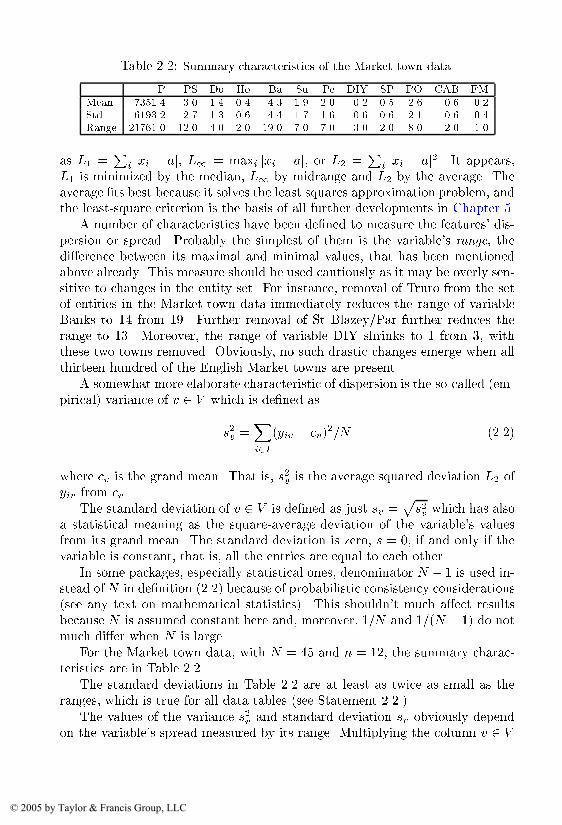
�� WHAT IS DATA
Table ���� Summary characteristics of the Market town data�
P PS Do Ho Ba Su Pe DIY SP PO CAB FMMean ����� ��� �� �� �� �� ��� ��� ��� ��� ��� ���Std ����� ��� ��� ��� � ��� ��� ��� ��� ��� ��� ��Range ������� ���� �� ��� ��� ��� ��� ��� ��� ��� ��� ���
as L� �P
i jxi � aj� L� � maxi jxi � aj� or L� �P
i jxi � aj�� It appears�L� is minimized by the median� L� by midrange and L� by the average� Theaverage ts best because it solves the least squares approximation problem� andthe leastsquare criterion is the basis of all further developments in Chapter ��A number of characteristics have been dened to measure the features� dis
persion or spread� Probably the simplest of them is the variable�s range� thedi erence between its maximal and minimal values� that has been mentionedabove already� This measure should be used cautiously as it may be overly sensitive to changes in the entity set� For instance� removal of Truro from the setof entities in the Market town data immediately reduces the range of variableBanks to �� from ��� Further removal of St Blazey�Par further reduces therange to ��� Moreover� the range of variable DIY shrinks to � from �� withthese two towns removed� Obviously� no such drastic changes emerge when allthirteen hundred of the English Market towns are present�A somewhat more elaborate characteristic of dispersion is the socalled �em
pirical� variance of v � V which is dened as
s�v �Xi�I
�yiv � cv���N �����
where cv is the grand mean� That is� s�v is the average squared deviation L� of
yiv from cv�The standard deviation of v � V is dened as just sv �
ps�v which has also
a statistical meaning as the squareaverage deviation of the variable�s valuesfrom its grand mean� The standard deviation is zero� s � �� if and only if thevariable is constant� that is� all the entries are equal to each other�In some packages� especially statistical ones� denominator N � � is used in
stead of N in denition ����� because of probabilistic consistency considerations�see any text on mathematical statistics�� This shouldn�t much a ect resultsbecause N is assumed constant here and� moreover� ��N and ���N � �� do notmuch di er when N is large�For the Market town data� with N � �� and n � ��� the summary charac
teristics are in Table ����The standard deviations in Table ��� are at least as twice as small as the
ranges� which is true for all data tables �see Statement ������The values of the variance s�v and standard deviation sv obviously depend
on the variable�s spread measured by its range� Multiplying the column v � V
© 2005 by Taylor & Francis Group, LLC
���� FEATURE CHARACTERISTICS ��
by � � � obviously multiplies its range and standard deviation by �� and thevariance by ���The quadratic index of spread� s�v � depends not only on the scale but also
on the character of the feature�s distribution within its range� Can we see how�Let as consider all quantitative variables dened on N entities i � I and
ranged between � and � inclusive� and analyze at what distributions the varianceattains its maximum and minimum values�It is not di�cult to see that any feature v that minimizes the variance s�v is
equal to � at one of the entities� � at another entity� and yiv � cv � ��� at allother entities i � I � The minimum variance s�v is
��N then�
Among the distributions under consideration� the maximum value of s�v isreached at a feature v which is binary� that is� has only boundary points� �and �� as its values� Indeed� if v has any other value at an entity i� then thevariance will only increase if we redene v in such a way that it becomes � or � ati depending on whether yiv is smaller or greater than v�s average cv � For a binaryv� let us specify proportion p of values yiv at which the feature is larger than itsgrand mean� yiv � cv� Then� obviously� the average cv � � ��� p� ! � p � pand� thus� s�v � ��� p�� ��� p� ! ��� p�� p � p��� p��The choice of the left and right bounds of the range� � and �� does have an
e ect on the values attained by the extremal variable but not on the conclusionof its binariness� That means that the following is proven�
Statement ���� With the range and proportion p of values smaller than theaverage prespeci�ed� the distribution at which the variance reaches its maximumis the distribution of a binary feature having p values at the left bound and ��pvalues at the right bound of the range�
Among the binary features� the maximum variance is reached at p � ����the maximum uncertainty� This implies one more property�
Statement ���� For any feature� its standard deviation is at least as twice assmall as its range�
Proof� Indeed� with the range being unity between � and �� the maximumvariance is p���p� � ��� at p � ��� leading to the maximum standard deviationof just half of the unity range� q�e�d�From the intuitive point of view� the range being the same� the greater the
variance the better the variable suits the task of clustering�
����� Categorical case
Let us rst consider binary features and then nominal ones�To quantitatively recode a binary feature� its Yes category is converted into
� and No into �� The grand mean of the obtained zero�one variable will be
© 2005 by Taylor & Francis Group, LLC
�� WHAT IS DATA
pv� the proportion of entities falling in the category Yes� Its variance will bes�v � p��� p��In statistics� two types of probabilistic mechanisms for generating zero�one
binary variables are considered� Bernoulli�binomial and Poisson� Each relies onhaving the proportion of ones� p� xed� However� the binomial distributionassumes that every single entry has the same probability p of being unity�whereas Poisson distribution does not care about individual entries� just thatthe proportion p of entries randomly thrown into a column must be unity� Thissubtle di erence makes the variance of the Poisson distribution greater� thevariance of the binomial distribution is equal to s�v � p��� p� and the varianceof the Poisson distribution is equal to �v � p� Thus� the variance of a onezerofeature considered as a quantitative feature corresponds to the statistical modelof binomial distribution�Turning to the case of nominal variables� let us denote the set of categories of
a nominal variable l by Vl� Any category v � Vl is conventionally characterizedby its frequency� the number of entities� Nv� falling in it� The sum of frequenciesis equal to the total number of entities in I �
Pv�Vl
Nv � N � The relativefrequencies� pv � Nv�N � sum up to unity� The vector p � �pv�� v � Vl is referredto as the distribution of l �over I�� A category with the largest frequency isreferred to as the distribution�s mode� The dispersion of a nominal variable l isfrequently measured by the socalled Gini coe�cient� or qualitative variance�
G �Xv�Vl
pv��� pv� � ��Xv�Vl
p�v �����
This is zero if all entities fall in one of the categories only� G is maximumwhen the distribution is uniform� that is� when all category frequencies are thesame� pv � ��jVlj for all v � Vl�A similar measure referred to as entropy and dened as
H � �Xv�Vl
pv log pv �����
with the logarithm�s base � is also quite popular� This measure is related tosocalled information theory ����� Entropy reaches its minimum and maximumvalues at the same distributions as the Gini coe�cient� Moreover� the Ginicoe�cient can be thought of as a linearized version of entropy since � � pvlinearly approximates log pv at pv close to �� In fact� both can be consideredaveraged information measures� just that one uses � log pv and the other ��pvto express the information contents�There exists a general formula to express the diversity of a nominal variable
as Sq � �� �P
v�Vlpqv���q � ��� q � � ������ The entropy and Gini index are
special cases of Sq since S� � G and S� � H assuming S� to be the limit of Sqwhen q tends to ��
© 2005 by Taylor & Francis Group, LLC
���� BIVARIATE ANALYSIS ��
A nominal variable l can be converted into a quantitative format by assigninga zero�one feature to each of its categories v � Vl coded by � or � dependingon whether an entity falls into the category or not� These binary features arereferred to sometimes as dummy variables�Unlike a binary feature� a twocategory nominal feature such as �Gender� is
converted into two columns� each corresponding to one of the categories� �Male�and �Female� of �Gender�� This way of quantization is quite convenient withinthe data recovery approach as will be seen further in section ��� and others�However� it is also compatible with the traditional view of quantitative measurement scales as expressed in terms of admissible transformations� Indeed�for a nominal scale x� any onetoone mapping y � ��x� is considered admissible� When there are only two categories� x� and x�� they can be recoded intoany y� and y� with an appropriate rescaling factor a and shift b so that thetransformation of x to y can be considered an a�ne one� y � ax! b� It is notdi�cult to prove that a � �y� � y����x� � x�� and b � �x�y� � x�y����x� � x��will do the recoding� In other words� nominal features with two categories canbe considered quantitative� The binary features� in this context� are those withcategory Yes coded by � and No by � for which transformation y � ax ! b ismeaningful only when a � ��The vector of averages of the dummy category features� pv� v � Vl� is
nothing but the distribution of l� Moreover� the Gini coe�cient appears tobe but the summary Bernoullian variance of the dummy category features�G �
Pv�Vl
pv�� � pv�� In the case when l has only two categories� this becomes just the variance of any of them doubled� Thus� the transformation ofa nominal variable into a bunch of zeroone dummies conveniently converts itinto a quantitative format which is compatible with the traditional treatmentof nominal features�
��� Bivariate analysis
Statistical science in the precomputer era developed a number of tools forthe analysis of interrelations between variables� which will be useful in thesequel� In the remainder of this section� a review is given of the three casesemerging from the pairwise considerations� with emphasis on the measurementscales� �a� quantitativetoquantitative� �b� categoricaltoquantitative� and �c�categoricaltocategorical variables� The discussion of the latter case followsthat in �����
����� Two quantitative variables
Mutual interrelations between two quantitative features can be caught witha scatter plot such as in Figure ����� page ��� Two indices for measuring
© 2005 by Taylor & Francis Group, LLC
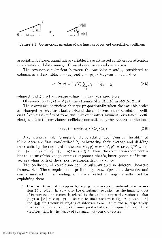
�� WHAT IS DATA
a
y
x
a0 ||y|| cos a cos a x/||x||
y/||y||
Figure ���� Geometrical meaning of the inner product and correlation coe�cient�
association between quantitative variables have attracted considerable attentionin statistics and data mining� those of covariance and correlation�
The covariance coe�cient between the variables x and y considered ascolumns in a data table� x � �xi� and y � �yi�� i � I � can be dened as
cov�x� y� � ���N�Xi�I
�xi � "x��yi � "y� �����
where "x and "y are the average values of x and y� respectively�Obviously� cov�x� x� � s��x�� the variance of x dened in section ������
The covariance coe�cient changes proportionally when the variable scalesare changed� A scaleinvariant version of the coe�cient is the correlation coe�cient �sometimes referred to as the Pearson productmoment correlation coe�cient� which is the covariance coe�cient normalized by the standard deviations�
r�x� y� � cov�x� y���s�x�s�y�� �����
A somewhat simpler formula for the correlation coe�cient can be obtainedif the data are rst standardized by subtracting their average and dividingthe results by the standard deviation� r�x� y� � cov�x�� y�� � �x�� y���N wherex�i � �xi� "x��s�x�� y�i � �yi� "y��s�y�� i � I � Thus� the correlation coe�cient isbut the mean of the componenttocomponent� that is� inner� product of featurevectors when both of the scales are standardized as above�The coe�cient of correlation can be substantiated in di erent theoretic
frameworks� These require some preliminary knowledge of mathematics andcan be omitted at rst reading� which is re�ected in using a smaller font forexplaining them�
�� Cosine� A geometric approach relying on concepts introduced later in sec�tion ����� o�ers the view that the covariance coe�cient as the inner productof feature column�vectors is related to the angle between the vectors so that�x� y � jjxjjjjyjj cos�x� y � This can be illustrated with Fig� ���� norms jjxjjand jjyjj are Euclidean lengths of intervals from to x and y respectively�The correlation coe�cient is the inner product of the corresponding normalizedvariables that is the cosine of the angle between the vectors�
© 2005 by Taylor & Francis Group, LLC
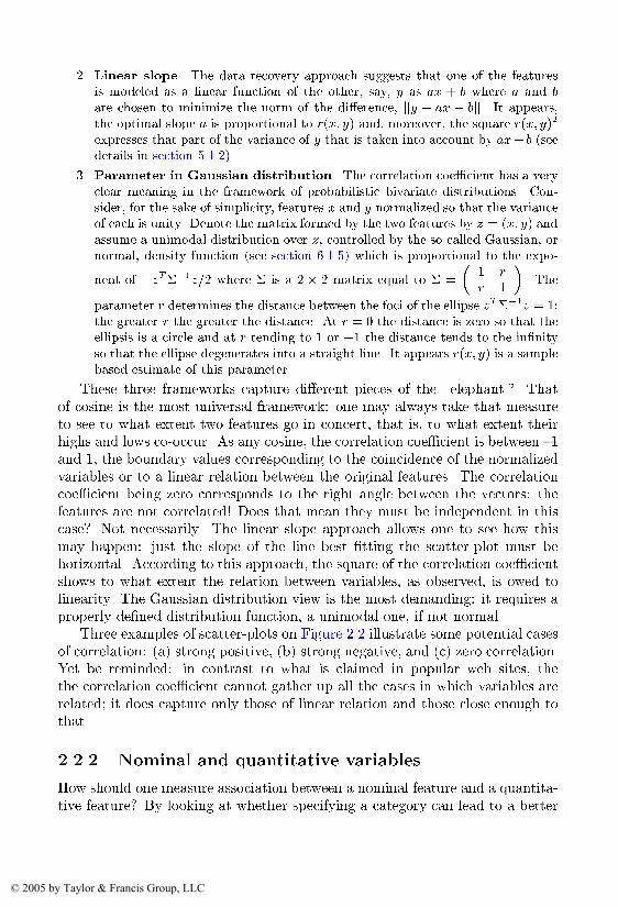
���� BIVARIATE ANALYSIS ��
�� Linear slope� The data recovery approach suggests that one of the featuresis modeled as a linear function of the other say y as ax � b where a and bare chosen to minimize the norm of the di�erence jjy � ax � bjj� It appearsthe optimal slope a is proportional to r�x� y and moreover the square r�x� y �
expresses that part of the variance of y that is taken into account by ax� b �seedetails in section ����� �
�� Parameter in Gaussian distribution� The correlation coe�cient has a veryclear meaning in the framework of probabilistic bivariate distributions� Con�sider for the sake of simplicity features x and y normalized so that the varianceof each is unity� Denote the matrix formed by the two features by z � �x� y andassume a unimodal distribution over z controlled by the so�called Gaussian ornormal density function �see section ����� which is proportional to the expo�
nent of �zT���z�� where � is a � � � matrix equal to � �
�� rr �
�� The
parameter r determines the distance between the foci of the ellipse zT���z � ��the greater r the greater the distance� At r � the distance is zero so that theellipsis is a circle and at r tending to � or �� the distance tends to the in�nityso that the ellipse degenerates into a straight line� It appears r�x� y is a samplebased estimate of this parameter�
These three frameworks capture di erent pieces of the �elephant�� Thatof cosine is the most universal framework� one may always take that measureto see to what extent two features go in concert� that is� to what extent theirhighs and lows cooccur� As any cosine� the correlation coe�cient is between ��and �� the boundary values corresponding to the coincidence of the normalizedvariables or to a linear relation between the original features� The correlationcoe�cient being zero corresponds to the right angle between the vectors� thefeatures are not correlated# Does that mean they must be independent in thiscase� Not necessarily� The linear slope approach allows one to see how thismay happen� just the slope of the line best tting the scatterplot must behorizontal� According to this approach� the square of the correlation coe�cientshows to what extent the relation between variables� as observed� is owed tolinearity� The Gaussian distribution view is the most demanding� it requires aproperly dened distribution function� a unimodal one� if not normal�Three examples of scatterplots on Figure ��� illustrate some potential cases
of correlation� �a� strong positive� �b� strong negative� and �c� zero correlation�Yet be reminded� in contrast to what is claimed in popular web sites� thethe correlation coe�cient cannot gather up all the cases in which variables arerelated� it does capture only those of linear relation and those close enough tothat�
����� Nominal and quantitative variables
How should one measure association between a nominal feature and a quantitative feature� By looking at whether specifying a category can lead to a better
© 2005 by Taylor & Francis Group, LLC
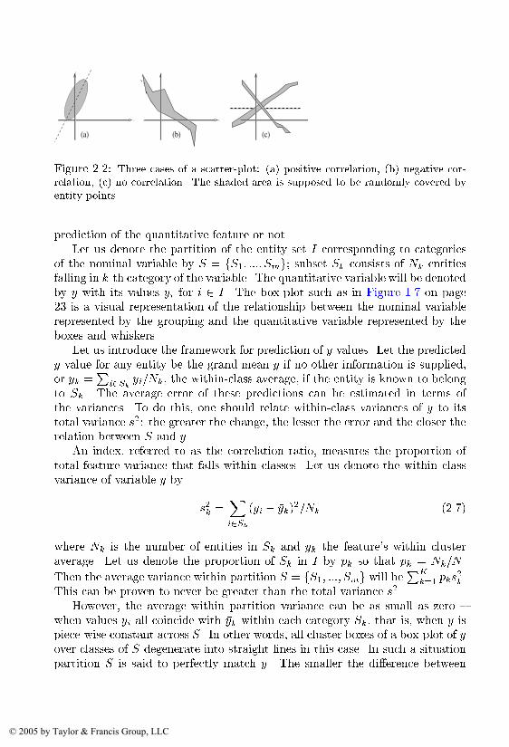
�� WHAT IS DATA
(a) (b) (c)
Figure ���� Three cases of a scatter�plot� �a positive correlation �b negative cor�relation �c no correlation� The shaded area is supposed to be randomly covered byentity points�
prediction of the quantitative feature or not�Let us denote the partition of the entity set I corresponding to categories
of the nominal variable by S � fS�� ���� Smg� subset Sk consists of Nk entitiesfalling in kth category of the variable� The quantitative variable will be denotedby y with its values yi for i � I � The boxplot such as in Figure ��� on page�� is a visual representation of the relationship between the nominal variablerepresented by the grouping and the quantitative variable represented by theboxes and whiskers�Let us introduce the framework for prediction of y values� Let the predicted
y value for any entity be the grand mean "y if no other information is supplied�or "yk �
Pi�Sk
yi�Nk� the withinclass average� if the entity is known to belongto Sk� The average error of these predictions can be estimated in terms ofthe variances� To do this� one should relate withinclass variances of y to itstotal variance s�� the greater the change� the lesser the error and the closer therelation between S and y�An index� referred to as the correlation ratio� measures the proportion of
total feature variance that falls within classes� Let us denote the within classvariance of variable y by
s�k �Xi�Sk
�yi � "yk���Nk �����
where Nk is the number of entities in Sk and "yk the feature�s within clusteraverage� Let us denote the proportion of Sk in I by pk so that pk � Nk�N �
Then the average variance within partition S � fS�� ���� Smg will bePK
k�� pks�k�
This can be proven to never be greater than the total variance s��However� the average within partition variance can be as small as zero �
when values yi all coincide with "yk within each category Sk� that is� when y ispiecewise constant across S� In other words� all cluster boxes of a boxplot of yover classes of S degenerate into straight lines in this case� In such a situationpartition S is said to perfectly match y� The smaller the di erence between
© 2005 by Taylor & Francis Group, LLC
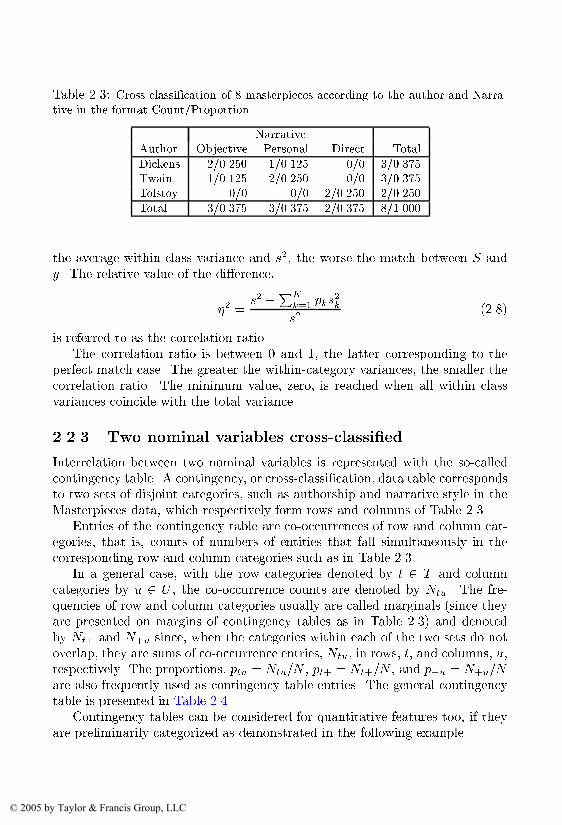
���� BIVARIATE ANALYSIS ��
Table ���� Cross�classi�cation of � masterpieces according to the author and Narra�tive in the format Count�Proportion�
NarrativeAuthor Objective Personal Direct Total
Dickens ����� ������ � ������Twain ������ ����� � ������Tolstoy � � ����� �����
Total ������ ������ ������ ����
the average withinclass variance and s�� the worse the match between S andy� The relative value of the di erence�
� �s� �PK
k�� pks�k
s������
is referred to as the correlation ratio�The correlation ratio is between � and �� the latter corresponding to the
perfect match case� The greater the withincategory variances� the smaller thecorrelation ratio� The minimum value� zero� is reached when all within classvariances coincide with the total variance�
����� Two nominal variables crossclassi�ed
Interrelation between two nominal variables is represented with the socalledcontingency table� A contingency� or crossclassication� data table correspondsto two sets of disjoint categories� such as authorship and narrative style in theMasterpieces data� which respectively form rows and columns of Table ����Entries of the contingency table are cooccurrences of row and column cat
egories� that is� counts of numbers of entities that fall simultaneously in thecorresponding row and column categories such as in Table ����In a general case� with the row categories denoted by t � T and column
categories by u � U � the cooccurrence counts are denoted by Ntu� The frequencies of row and column categories usually are called marginals �since theyare presented on margins of contingency tables as in Table ���� and denotedby Nt� and N�u since� when the categories within each of the two sets do notoverlap� they are sums of cooccurrence entries� Ntu� in rows� t� and columns� u�respectively� The proportions� ptu � Ntu�N � pt� � Nt��N � and p�u � N�u�Nare also frequently used as contingency table entries� The general contingencytable is presented in Table ����Contingency tables can be considered for quantitative features too� if they
are preliminarily categorized as demonstrated in the following example�
© 2005 by Taylor & Francis Group, LLC
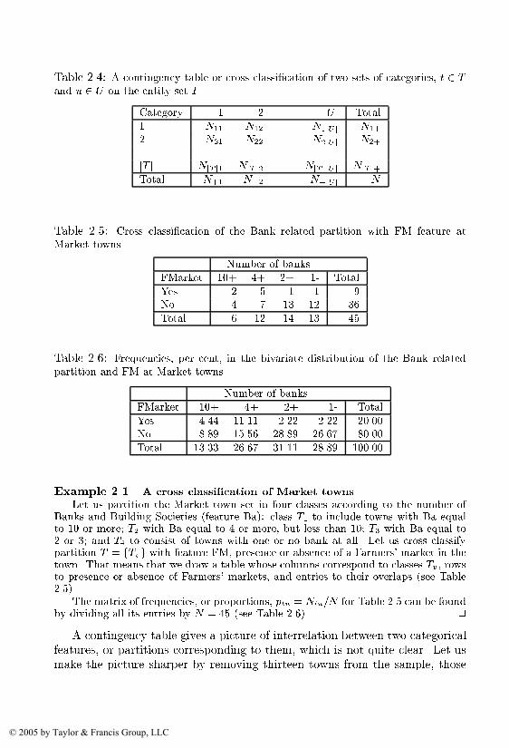
�� WHAT IS DATA
Table ���� A contingency table or cross classi�cation of two sets of categories t � Tand u � U on the entity set I�
Category � � ��� jU j Total
� N�� N�� ��� N�jUj N��
� N�� N�� ��� N�jUj N��
��� ��� ��� ���� ��� ���jT j NjT j� NjT j� ��� NjT jjUj NjT j�
Total N�� N�� ��� N�jUj N
Table ���� Cross classi�cation of the Bank related partition with FM feature atMarket towns�
Number of banks
FMarket �� �� �� �� Total
Yes � � � � �No � � �� �� ��
Total � �� �� �� ��
Table ���� Frequencies per cent in the bivariate distribution of the Bank relatedpartition and FM at Market towns�
Number of banks
FMarket �� �� �� �� Total
Yes ���� ����� ���� ���� ��No ���� ����� ����� ����� ��
Total ����� ����� ����� ����� ��
Example ���� A cross classi�cation of Market towns
Let us partition the Market town set in four classes according to the number ofBanks and Building Societies �feature Ba � class T� to include towns with Ba equalto � or more� T� with Ba equal to � or more but less than �� T� with Ba equal to� or �� and T� to consist of towns with one or no bank at all� Let us cross classifypartition T � fTvg with feature FM presence or absence of a Farmers� market in thetown� That means that we draw a table whose columns correspond to classes Tv rowsto presence or absence of Farmers� markets and entries to their overlaps �see Table��� �
The matrix of frequencies or proportions ptu � Ntu�N for Table ��� can be foundby dividing all its entries by N � �� �see Table ��� � �
A contingency table gives a picture of interrelation between two categoricalfeatures� or partitions corresponding to them� which is not quite clear� Let usmake the picture sharper by removing thirteen towns from the sample� those
© 2005 by Taylor & Francis Group, LLC

���� BIVARIATE ANALYSIS ��
Table ���� Cross classi�cation of the Bank related partition with FM feature at a�cleaned� subsample of Market towns�
Number of banks
FMarket �� �� �� �� Total
Yes � � �No �� �� ��
Total � � �� �� ��
falling in the less populated cells of Table ��� �see Table ����� Table ��� showsa very clear association between two features on the �cleaned� subsample� theFarmers� markets are present only in towns in which the number of banks is� or greater� A somewhat subtler relation� the medium numbers of banks aremore closly associated with the presence of a Farmers� market than the higherones�This clear picture is somewhat blurred in the original sample in Table ���
and� moreover� maybe does not hold at all�Thus� the issue of relating two features to each other can be addressed by
looking at mismatches� For instance� Table ��� shows that Narrative style isquite close to authorship� though they do not completely match� there are twomismatching entities� one by Dickens and the other by Twain� Similarly� thereare �� mismatches in Table ��� removed in Table ���� The sheer numbers ofmismatching entities measure the di erences between category sets rather wellwhen the distribution of entities within each category is rather uniform as it isin Table ���� When the proportions of entities in di erent categories drasticallydi er� as in Table ���� to measure association between category sets more properly� the numbers of mismatching entities should be weighted according to thefrequencies of corresponding categories� Can we discover the relation in Table��� without removing entities�To measure association between categories according to a contingency table�
a founding father of the science of statistics� A� Quetelet� proposed utilizing therelative or absolute change of the conditional probability of a category� Theconditional probability p�u�t� � Ntu�Nt� � ptu�pt� measures the proportionof category u in category t� Quetelet coe�cients measure the di erence betweenp�u�t� and the average rate p�u of u � U � The Quetelet absolute probabilitychange is dened as
gtu � p�u�t�� p�u � �ptu � pt�p�u��pt�� �����
and the Quetelet relative change
qtu � gtu�p�u � ptu��pt�p�u�� � � �ptu � pt�p�u���pt�p�u� ������
© 2005 by Taylor & Francis Group, LLC
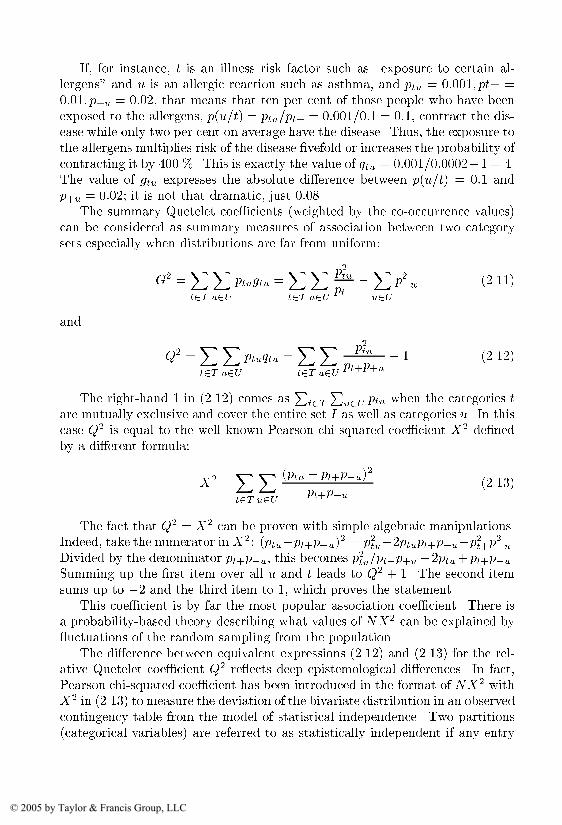
�� WHAT IS DATA
If� for instance� t is an illness risk factor such as �exposure to certain allergens� and u is an allergic reaction such as asthma� and ptu � ������ pt! ������ p�u � ����� that means that ten per cent of those people who have beenexposed to the allergens� p�u�t� � ptu�pt� � ��������� � ���� contract the disease while only two per cent on average have the disease� Thus� the exposure tothe allergens multiplies risk of the disease vefold or increases the probability ofcontracting it by ��� � This is exactly the value of qtu � �������������� � ��The value of gtu expresses the absolute di erence between p�u�t� � ��� andp�u � ����� it is not that dramatic� just �����The summary Quetelet coe�cients �weighted by the cooccurrence values�
can be considered as summary measures of association between two categorysets especially when distributions are far from uniform�
G� �Xt�T
Xu�U
ptugtu �Xt�T
Xu�U
p�tupt�
�Xu�U
p��w ������
and
Q� �Xt�T
Xu�U
ptuqtu �Xt�T
Xu�U
p�tupt�p�u
� � ������
The righthand � in ������ comes asP
t�T
Pu�U ptu when the categories t
are mutually exclusive and cover the entire set I as well as categories u� In thiscase Q� is equal to the well known Pearson chisquared coe�cient X� denedby a di erent formula�
X� �Xt�T
Xu�U
�ptu � pt�p�u��
pt�p�u������
The fact that Q� � X� can be proven with simple algebraic manipulations�Indeed� take the numerator in X�� �ptu�pt�p�u�� � p�tu��ptupt�p�u!p�t�p��u�Divided by the denominator pt�p�u� this becomes p
�tu�pt�p�u��ptu!pt�p�u�
Summing up the rst item over all u and t leads to Q� ! �� The second itemsums up to �� and the third item to �� which proves the statement�This coe�cient is by far the most popular association coe�cient� There is
a probabilitybased theory describing what values of NX� can be explained by�uctuations of the random sampling from the population�The di erence between equivalent expressions ������ and ������ for the rel
ative Quetelet coe�cient Q� re�ects deep epistemological di erences� In fact�Pearson chisquared coe�cient has been introduced in the format of NX� withX� in ������ to measure the deviation of the bivariate distribution in an observedcontingency table from the model of statistical independence� Two partitions�categorical variables� are referred to as statistically independent if any entry
© 2005 by Taylor & Francis Group, LLC
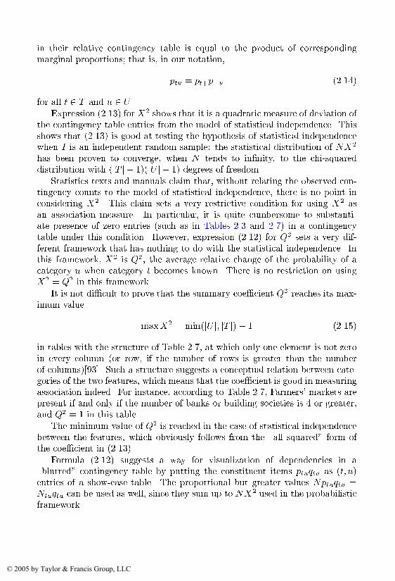
���� BIVARIATE ANALYSIS ��
in their relative contingency table is equal to the product of correspondingmarginal proportions� that is� in our notation�
ptu � pt�p�u ������
for all t � T and u � U �Expression ������ for X� shows that it is a quadratic measure of deviation of
the contingency table entries from the model of statistical independence� Thisshows that ������ is good at testing the hypothesis of statistical independencewhen I is an independent random sample� the statistical distribution of NX�
has been proven to converge� when N tends to innity� to the chisquareddistribution with �jT j � ���jU j � �� degrees of freedom�Statistics texts and manuals claim that� without relating the observed con
tingency counts to the model of statistical independence� there is no point inconsidering X�� This claim sets a very restrictive condition for using X� asan association measure� In particular� it is quite cumbersome to substantiate presence of zero entries �such as in Tables ��� and ���� in a contingencytable under this condition� However� expression ������ for Q� sets a very different framework that has nothing to do with the statistical independence� Inthis framework� X� is Q�� the average relative change of the probability of acategory u when category t becomes known� There is no restriction on usingX� � Q� in this framework�
It is not di�cult to prove that the summary coe�cient Q� reaches its maximum value
maxX� � min�jU j� jT j�� � ������
in tables with the structure of Table ���� at which only one element is not zeroin every column �or row� if the number of rows is greater than the numberof columns������ Such a structure suggests a conceptual relation between categories of the two features� which means that the coe�cient is good in measuringassociation indeed� For instance� according to Table ���� Farmers� markets arepresent if and only if the number of banks or building societies is � or greater�and Q� � � in this table�The minimum value of Q� is reached in the case of statistical independence
between the features� which obviously follows from the �all squared� form ofthe coe�cient in �������
Formula ������ suggests a way for visualization of dependencies in a�blurred� contingency table by putting the constituent items ptuqtu as �t� u�entries of a showcase table� The proportional but greater values Nptuqtu �Ntuqtu can be used as well� since they sum up to NX� used in the probabilisticframework�
© 2005 by Taylor & Francis Group, LLC

�� WHAT IS DATA
Table ���� Relative Quetelet coe�cients per cent for Table ����
Number of banksFMarket �� �� �� ��
Yes ����� ������ ������ ������No ������ ����� ����� ����
Table ���� Items summed up in the chi�square contingency coe�cient �times N inthe Quetelet format ����� for Table ����
Number of banksFMarket �� �� �� �� Total
Yes ���� �� ���� ���� ����No ���� ���� ���� ��� ����
Total ��� ���� ���� ���� ����
Example ���� Highlighting positive contributions to the total association
The table of the relative Quetelet coe�cients qtu for Table ��� is presented inTable ��� and that of items Ntuqtu in Table ����
It is easy to see that the highlighted positive entries in both of the tables expressthe same pattern as in Table ��� but without removing entities from the table�
Table ��� demonstrates one more property of the items ptuqtu summed up in thechi�square coe�cient� their within�row or within�column sums are always positive� �
Highlighting the positive entries ptuqtu � � �or qtu � �� can be used forvisualization of the pattern of association between any categorical features �����
A similar to ������� though asymmetric� expression can be derived for G��
G� �Xt�T
Xu�U
�ptu � pt�p�u��
pt�������
Though it also can be considered a measure of deviation of the contingencytable from the model of statistical independence� G� has been always consideredin the literature as a measure of association� A corresponding denition involvesthe Gini coe�cient dened in section ������ G�U� � � �Pu�U p
��u� Within a
category t� the variation is equal to G�U�t� � � �Pu�U �ptu�pt���� which
makes� on average� the qualitative variation that cannot be explained by T �G�U�T � �
Pt�T pt�G�U�t� � ��
Pt�T
Pu�U p
�tu�pt��
The di erence G�U��G�U�T � represents that part ofG�U� that is explainedby T � and this is exactly G� in �������
© 2005 by Taylor & Francis Group, LLC
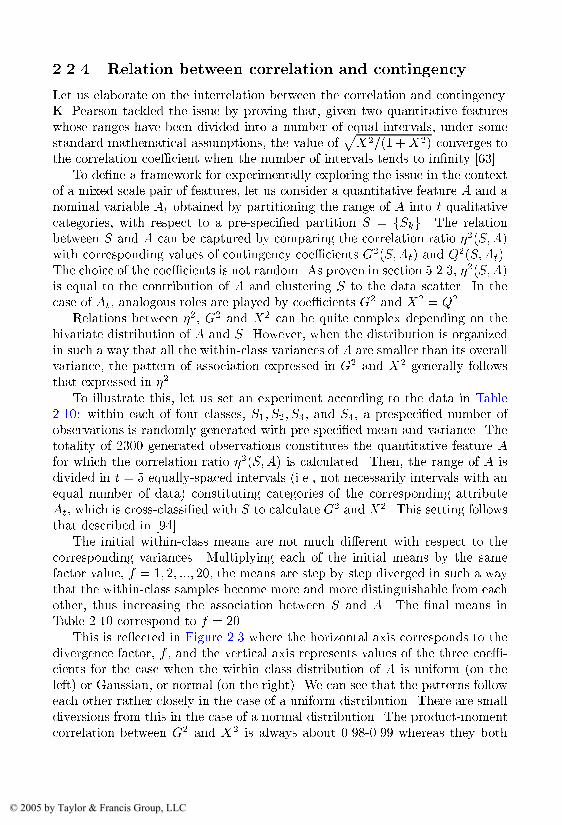
���� BIVARIATE ANALYSIS ��
����� Relation between correlation and contingency
Let us elaborate on the interrelation between the correlation and contingency�K� Pearson tackled the issue by proving that� given two quantitative featureswhose ranges have been divided into a number of equal intervals� under somestandard mathematical assumptions� the value of
pX���� !X�� converges to
the correlation coe�cient when the number of intervals tends to innity �����To dene a framework for experimentally exploring the issue in the context
of a mixed scale pair of features� let us consider a quantitative feature A and anominal variable At obtained by partitioning the range of A into t qualitativecategories� with respect to a prespecied partition S � fSkg� The relationbetween S and A can be captured by comparing the correlation ratio ��S�A�with corresponding values of contingency coe�cients G��S�At� and Q
��S�At��The choice of the coe�cients is not random� As proven in section ������ ��S�A�is equal to the contribution of A and clustering S to the data scatter� In thecase of At� analogous roles are played by coe�cients G
� and X� � Q��Relations between �� G� and X� can be quite complex depending on the
bivariate distribution of A and S� However� when the distribution is organizedin such a way that all the withinclass variances of A are smaller than its overallvariance� the pattern of association expressed in G� and X� generally followsthat expressed in ��To illustrate this� let us set an experiment according to the data in Table
����� within each of four classes� S�� S�� S�� and S�� a prespecied number ofobservations is randomly generated with prespecied mean and variance� Thetotality of ���� generated observations constitutes the quantitative feature Afor which the correlation ratio ��S�A� is calculated� Then� the range of A isdivided in t � � equallyspaced intervals �i�e�� not necessarily intervals with anequal number of data� constituting categories of the corresponding attributeAt� which is crossclassied with S to calculate G
� and X�� This setting followsthat described in �����The initial withinclass means are not much di erent with respect to the
corresponding variances� Multiplying each of the initial means by the samefactor value� f � �� �� ���� ��� the means are step by step diverged in such a waythat the withinclass samples become more and more distinguishable from eachother� thus increasing the association between S and A� The nal means inTable ���� correspond to f � ���This is re�ected in Figure ��� where the horizontal axis corresponds to the
divergence factor� f � and the vertical axis represents values of the three coe�cients for the case when the within class distribution of A is uniform �on theleft� or Gaussian� or normal �on the right�� We can see that the patterns followeach other rather closely in the case of a uniform distribution� There are smalldiversions from this in the case of a normal distribution� The productmomentcorrelation between G� and X� is always about �������� whereas they both
© 2005 by Taylor & Francis Group, LLC
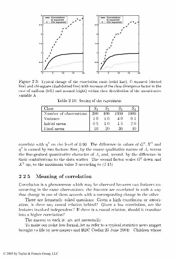
�� WHAT IS DATA
0 5 10 15 200
0.5
1
1.5
2
2.5
3CorrelationG squaredChi squared
0 5 10 15 200
0.5
1
1.5
2
2.5
3CorrelationG squaredChi squared
Figure ���� Typical change of the correlation ratio �solid line G squared �dottedline and chi�square �dashdotted line with increase of the class divergence factor in thecase of uniform �left and normal �right within class distribution of the quantitativevariable A�
Table ����� Setting of the experiment�
Class S� S� S� S�Number of observations ��� ��� ���� ����Variance ��� ��� ��� ���Initial mean ��� ��� ��� ���Final mean �� �� �� ��
correlate with � on the level of ����� The di erence in values of G�� X� and� is caused by two factors� rst� by the coarse qualitative nature of At versusthe negrained quantitative character of A� and� second� by the di erence intheir contributions to the data scatter� The second factor scales G� down andX� up� to the maximum value � according to �������
����� Meaning of correlation
Correlation is a phenomenon which may be observed between two features cooccurring in the same observations� the features are corelated in such a waythat change in one of them accords with a corresponding change in the other�These are frequently asked questions� Given a high correlation or associ
ation� is there any causal relation behind� Given a low correlation� are thefeatures involved independent� If there is a causal relation� should it translateinto a higher correlation�The answer to each is� no� not necessarily�To make our point less formal� let us refer to a typical statistics news nugget
brought to life by newspapers and BBC Ceefax �� June ����� �Children whose
© 2005 by Taylor & Francis Group, LLC
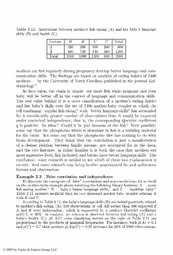
���� BIVARIATE ANALYSIS ��
Table ����� Association between mother�s �sh eating �A and her baby�s languageskills �B and health �C �
Feature B �B C �C Total
A �� �� �� �� ��A �� �� �� �� ��
Total � � �� � �
mothers eat sh regularly during pregnancy develop better language and communication skills� The ndings are based on analysis of eating habits of ����mothers ��� by the University of North Carolina� published in the journal Epidemiology��
At face value� the claim is simple� eat more sh while pregnant and yourbaby will be better o in the contest of language and communication skills�The real value behind it is a cross classication of a mother�s eating habitsand her baby�s skills over the set of ���� motherbaby couples at which thecell combining �regular sh eating� with �better language skills� has accountedfor a considerably greater number of observations than it would be expectedunder statistical independence� that is� the corresponding Quetelet coe�cientq is positive� So what� Could it be just because of the sh� Very possibly�some say that the phosphorus which is abundant in sh is a building materialfor the brain� Yet some say that the phosphorus diet has nothing to do withbrain development� They think that the correlation is just a manifestationof a deeper relation between family income� not accounted for in the data�and the two features� in richer families it is both the case that mothers eatmore expensive food� sh included� and babies have better language skills� Theconclusion� more research is needed to see which of these two explanations iscorrect� And more research may bring further unaccounted for and unforeseenfactors and observations�
Example ���� False correlation and independence
To illustrate the emergence of �false� correlations and non�correlations let us dwellon the mother�baby example above involving the following binary features� A � �more�sh eating mother� B � �baby�s better language skills� and C � �healthier baby��Table ���� presents arti�cial data on two thousand mother�baby couples relating Awith B and C�
According to Table ���� the baby�s language skills �B are indeed positively relatedto mother�s �sh eating �A � �� observations at cell AB rather than � expected ifA and B were independent which is supported by a positive Quetelet coe�cientq�B�A � ��� In contrast no relation is observed between �sh eating �A and ababy�s health �C � all A�C cross classifying entries on the right of Table ���� areproportional to the products of marginal frequencies� For instance with p�A � ��and p�C � �� their product p�A p�C � ��� accounts for ��� of � observations
© 2005 by Taylor & Francis Group, LLC
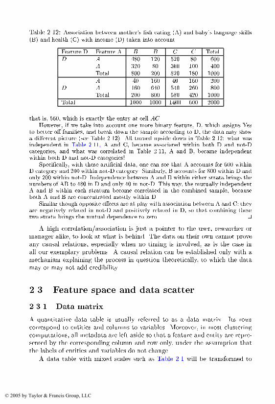
�� WHAT IS DATA
Table ����� Association between mother�s �sh eating �A and baby�s language skills�B and health �C with income �D taken into account�
Feature D Feature A B �B C �C Total
D A �� �� �� � ��A �� � � � �Total � � �� �� �
A � �� � �� ��D �A �� �� �� �� �
Total � � �� �� �
Total � � �� � �
that is �� which is exactly the entry at cell AC�However if we take into account one more binary feature D which assigns Yes
to better o� families and break down the sample according to D the data may showa di�erent picture �see Table ���� � All turned upside down in Table ����� what wasindependent in Table ���� A and C became associated within both D and not�Dcategories and what was correlated in Table ���� A and B became independentwithin both D and not�D categories�
Speci�cally with these arti�cial data one can see that A accounts for � withinD category and � within not�D category� Similarly B accounts for � within D andonly � within not�D� Independence between A and B within either strata brings thenumbers of AB to �� in D and only � in not�D� This way the mutually independentA and B within each stratum become correlated in the combined sample becauseboth A and B are concentrated mostly within D�
Similar though opposite e�ects are at play with association between A and C� theyare negatively related in not�D and positively related in D so that combining thesetwo strata brings the mutual dependence to zero� �
A high correlation�association is just a pointer to the user� researcher ormanager alike� to look at what is behind� The data on their own cannot proveany causal relations� especially when no timing is involved� as is the case inall our exemplary problems� A causal relation can be established only with amechanism explaining the process in question theoretically� to which the datamay or may not add credibility�
��� Feature space and data scatter
����� Data matrix
A quantitative data table is usually referred to as a data matrix� Its rowscorrespond to entities and columns to variables� Moreover� in most clusteringcomputations� all metadata are left aside so that a feature and entity are represented by the corresponding column and row only� under the assumption thatthe labels of entities and variables do not change�
A data table with mixed scales such as Table ��� will be transformed to
© 2005 by Taylor & Francis Group, LLC
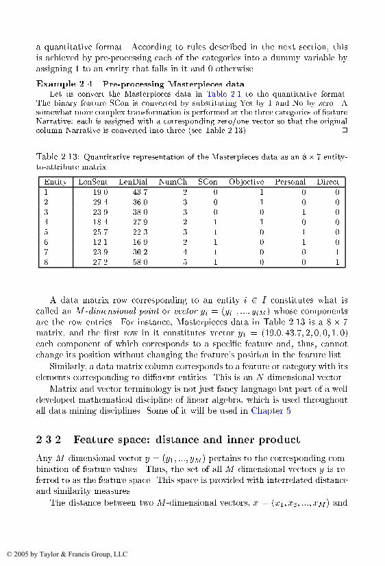
���� FEATURE SPACE AND DATA SCATTER ��
a quantitative format� According to rules described in the next section� thisis achieved by preprocessing each of the categories into a dummy variable byassigning � to an entity that falls in it and � otherwise�
Example ���� Pre processing Masterpieces data
Let us convert the Masterpieces data in Table ��� to the quantitative format�The binary feature SCon is converted by substituting Yes by � and No by zero� Asomewhat more complex transformation is performed at the three categories of featureNarrative� each is assigned with a corresponding zero�one vector so that the originalcolumn Narrative is converted into three �see Table ���� � �
Table ����� Quantitative representation of the Masterpieces data as an �� � entity�to�attribute matrix�
Entity LenSent LenDial NumCh SCon Objective Personal Direct
� ��� ���� � � � ���� ��� � � � ���� ��� � � � ���� ���� � � � � ���� ���� � � � � ���� ���� � � � � ���� ��� � � �� ���� ��� � � �
A data matrix row corresponding to an entity i � I constitutes what iscalled an M�dimensional point or vector yi � �yi�� ���� yiM � whose componentsare the row entries� For instance� Masterpieces data in Table ���� is a � �matrix� and the rst row in it constitutes vector y� � ������ ����� �� �� �� �� ��each component of which corresponds to a specic feature and� thus� cannotchange its position without changing the feature�s position in the feature list�
Similarly� a data matrix column corresponds to a feature or category with itselements corresponding to di erent entities� This is an N dimensional vector�
Matrix and vector terminology is not just fancy language but part of a welldeveloped mathematical discipline of linear algebra� which is used throughoutall data mining disciplines� Some of it will be used in Chapter ��
����� Feature space� distance and inner product
Any M dimensional vector y � �y�� ���� yM � pertains to the corresponding combination of feature values� Thus� the set of all M dimensional vectors y is referred to as the feature space� This space is provided with interrelated distanceand similarity measures�
The distance between two M dimensional vectors� x � �x�� x�� ���� xM � and
© 2005 by Taylor & Francis Group, LLC
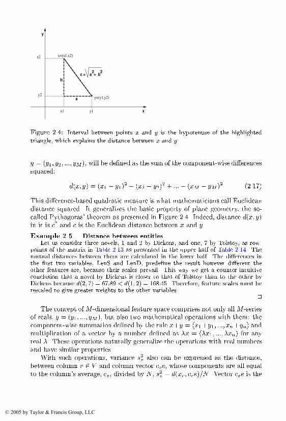
�� WHAT IS DATA
a + b2 2
x2
y2
x1 y1
y=(y1,y2)
x=(x1,x2)
a
b
y
x
c =
Figure ���� Interval between points x and y is the hypotenuse of the highlighted
triangle which explains the distance between x and y�
y � �y�� y�� ���� yM �� will be dened as the sum of the componentwise di erencessquared�
d�x� y� � �x� � y��� ! �x� � y��
� ! ���! �xM � yM �� ������
This di erencebased quadratic measure is what mathematicians call Euclideandistance squared� It generalizes the basic property of plane geometry� the socalled Pythagoras� theorem as presented in Figure ���� Indeed� distance d�x� y�in it is c� and c is the Euclidean distance between x and y�
Example ���� Distance between entitiesLet us consider three novels � and � by Dickens and one � by Tolstoy as row�
points of the matrix in Table ���� as presented in the upper half of Table ����� Themutual distances between them are calculated in the lower half� The di�erences inthe �rst two variables LenS and LenD prede�ne the result however di�erent theother features are because their scales prevail� This way we get a counter�intuitiveconclusion that a novel by Dickens is closer to that of Tolstoy than to the other byDickens because d��� � � ����� � d��� � � ������� Therefore feature scales must berescaled to give greater weights to the other variables�
�
The concept ofM dimensional feature space comprises not only allM seriesof reals� y � �y�� ���� yM �� but also two mathematical operations with them� thecomponentwise summation dened by the rule x!y � �x�!y�� ���� xn!yn� andmultiplication of a vector by a number dened as x � �x�� ���� xn� for anyreal � These operations naturally generalize the operations with real numbersand have similar properties�With such operations� variance s�v also can be expressed as the distance�
between column v � V and column vector cve� whose components are all equalto the column�s average� cv� divided by N � s
�v � d�xv � cve��N � Vector cve is the
© 2005 by Taylor & Francis Group, LLC
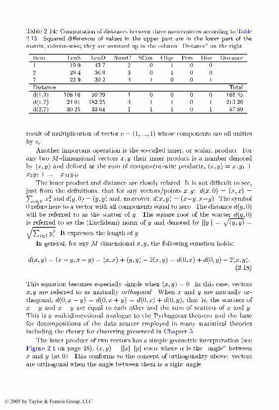
���� FEATURE SPACE AND DATA SCATTER ��
Table ����� Computation of distances between three masterpieces according to Table����� Squared di�erences of values in the upper part are in the lower part of thematrix column�wise� they are summed up in the column �Distance� on the right�
Item LenS LenD NumC SCon Obje Pers Dire Distance
� ��� ���� � � � ���� ��� � � � ���� ��� � � �
Distance Total
d��� ����� ����� � ������d��� ���� ������ � � � � ������d��� ���� ����� � � � � �����
result of multiplication of vector e � ��� ���� �� whose components are all unitiesby cv �
Another important operation is the socalled inner� or scalar� product� Forany two M dimensional vectors x� y their inner product is a number denotedby �x� y� and dened as the sum of componentwise products� �x� y� � x�y� !x�y� ! ���! xMyM �
The inner product and distance are closely related� It is not di�cult to see�just from the denitions� that for any vectors�points x� y� d�x� �� � �x� x� �P
v�V x�v and d�y� �� � �y� y� and� moreover� d�x� y� � �x�y� x�y�� The symbol
� refers here to a vector with all components equal to zero� The distance d�y� ��will be referred to as the scatter of y� The square root of the scatter d�y� ��is referred to as the �Euclidean� norm of y and denoted by jjyjj � p�y� y� �qP
i�I y�i � It expresses the length of y�
In general� for any M dimensional x� y� the following equation holds�
d�x� y� � �x� y� x� y� � �x� x� ! �y� y�� ��x� y� � d��� x� ! d��� y�� ��x� y��������
This equation becomes especially simple when �x� y� � �� In this case� vectorsx� y are referred to as mutually orthogonal� When x and y are mutually orthogonal� d��� x � y� � d��� x ! y� � d��� x� ! d��� y�� that is� the scatters ofx � y and x ! y are equal to each other and the sum of scatters of x and y�This is a multidimensional analogue to the Pythagoras theorem and the basefor decompositions of the data scatter employed in many statistical theoriesincluding the theory for clustering presented in Chapter ��
The inner product of two vectors has a simple geometric interpretation �seeFigure ��� on page ���� �x� y� � jjxjjjjyjj cos� where � is the �angle� betweenx and y �at ��� This conforms to the concept of orthogonality above� vectorsare orthogonal when the angle between them is a right angle�
© 2005 by Taylor & Francis Group, LLC
�� WHAT IS DATA
����� Data scatter
The summary scatter of all rowvectors in data matrix Y is referred to as thedata scatter of Y and denoted by
T �Y � �Xi�I
d��� yi� �Xi�I
Xv�V
y�iv ������
Equation ������ means that T �Y � is the total of all Y entries squared�An important characteristic of feature v � V is its contribution to the data
scatter dened as
Tv �Xi�I
y�iv � ������
the distance of the N dimensional column from the zero column� Data scatteris obviously the sum of contributions of all variables� T �Y � �
Pv�V Tv�
If feature v is centered� then its contribution to the data scatter is proportional to its variance�
Tv � Ns�v ������
Indeed� cv � � since v is centered� Thus� s�v �
Pi�I �yiv � ����N � Tv�N �
The relative contribution Tv�T �Y � is a characteristic playing an importantrole in data standardization issues as explained in the next section�
��� Pre�processing and standardizing mixed
data
The data preprocessing stage is to transform the raw entitytofeature tableinto a quantitative matrix for further analysis� To do this� one needs rst toconvert all categorical data to a numerical format� We will do this by using adummy zeroone variable for each category� Then variables are standardized byshifting their origins and rescaling� This operation can be clearly substantiatedfrom a statistics perspective� typically� by assuming that entities have beenrandomly sampled from an underlying Gaussian distribution� In data mining�substantiation may come from the data geometry� By shifting all the origins tofeature means� entities become scattered around the center of gravity so thatclusters can be more easily �seen� from that point� With feature rescaling�feature scales become balanced according to the principle of equal importanceof each feature brought into the data table�To implement these general principles� we are going to rely on the following
threestage procedure� The stages are� ��� enveloping qualitative categories���� standardization� and ��� rescaling� as follows�
© 2005 by Taylor & Francis Group, LLC
���� PRE�PROCESSING AND STANDARDIZING MIXED DATA ��
�� Quantitatively enveloping categories� This stage is to convert amixed scale data table into a quantitative matrix by treating every qualitative category as a separate dummy variable coded by � or � dependingon whether an entity falls into the category or not� Binary features arecoded similarly except that no additional columns are created� Quantitative features are left as they are� The converted data table will be denotedby X � �xiv�� i � I� v � V �
�� Standardization� This stage aims at transforming featurecolumns ofthe data matrix to make them comparable by shifting their origins toav and rescaling them by bv� v � V � thus to create standardized matrixY � �yiv��
yiv �xiv � av
bv� i � I� v � V� ������
In this text� the shift coe�cient av always will be the grand mean� Inparticular� the dummy variable corresponding to category v � Vl has itsmean cv � pv� the proportion of entities falling in the category�
The scale factor bv can be either the standard deviation or range or otherquantity re�ecting the variable�s spread� In particular� for a categoryv � Vl� the standard deviation can be either
ppv��� pv� �Bernoulli dis
tribution� orppv �Poisson distribution�� see page ��� The range of a
dummy variable is always ��
Using the standard deviation is popular in data mining probably becauseit is used in classical statistics relying on the theory of Gaussian distribution which is characterized by the mean and standard deviation� Thusstandardized� contributions of all features to data scatter become equal toeach other because of the proportionality of contributions and standarddeviations� On rst glance this seems an attractive property guaranteeingequal contributions of all features to the results� an opinion to which thecurrent author once also subscribed ����� However� this is not so� Twodi erent factors contribute to the value of standard deviation� the featurescale and the shape of its distribution� As shown in section ������ withinthe same range scale the standard deviation may greatly vary from theminimum� at the peak unimodal distribution� to the maximum� at thepeak bimodal distribution� By standardizing with standard deviations�we deliberately bias data in favor of unimodal distributions� although obviously it is the bimodal distribution that should contribute to clusteringmost� This is why the range� not the standard deviation� is used here asthe scaling factor bv� In the case when there can be outliers in data� whichmay highly a ect the range� another more stable rangelike scaling factorcan be chosen� such as the di erence between percentiles� that does not
© 2005 by Taylor & Francis Group, LLC
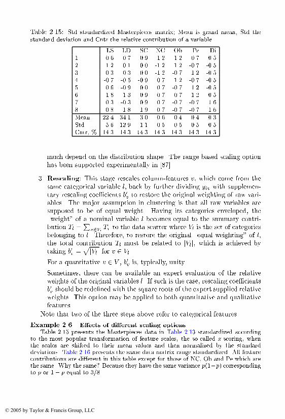
�� WHAT IS DATA
Table ����� Std standardized Masterpieces matrix� Mean is grand mean Std thestandard deviation and Cntr the relative contribution of a variable�
LS LD SC NC Ob Pe Di� ��� �� ��� ���� ��� ��� ���� ��� �� � ���� ��� ��� ���� �� �� � ���� ��� ��� ���� ��� ��� ��� �� ��� ��� ���� �� ��� � �� ��� ��� ���� ���� ���� ��� �� ��� ��� ���� �� ��� �� �� ��� ��� ���� �� ��� ��� �� ��� ��� ���
Mean ���� ���� �� �� �� �� ��Std ��� ���� ��� �� �� �� ��Cntr � ���� ���� ���� ���� ���� ���� ����
much depend on the distribution shape� The range based scaling optionhas been supported experimentally in �����
�� Rescaling� This stage rescales columnfeatures v� which come from thesame categorical variable l� back by further dividing yiv with supplementary rescaling coe�cients b�v to restore the original weighting of raw variables� The major assumption in clustering is that all raw variables aresupposed to be of equal weight� Having its categories enveloped� the�weight� of a nominal variable l becomes equal to the summary contribution Tl �
Pv�Vl
Tv to the data scatter where Vl is the set of categoriesbelonging to l� Therefore� to restore the original �equal weighting� of l�the total contribution Tl must be related to jVlj� which is achieved bytaking b�v �
pjVlj for v � Vl�
For a quantitative v � V � b�v is� typically� unity�
Sometimes� there can be available an expert evaluation of the relativeweights of the original variables l� If such is the case� rescaling coe�cientsb�v should be redened with the square roots of the expert supplied relativeweights� This option may be applied to both quantitative and qualitativefeatures�
Note that two of the three steps above refer to categorical features�
Example ���� E�ects of di�erent scaling optionsTable ���� presents the Masterpieces data in Table ���� standardized according
to the most popular transformation of feature scales the so�called z�scoring whenthe scales are shifted to their mean values and then normalized by the standarddeviations� Table ���� presents the same data matrix range standardized� All featurecontributions are di�erent in this table except for those of NC Ob and Pe which arethe same� Why the same� Because they have the same variance p���p correspondingto p or � � p equal to ����
© 2005 by Taylor & Francis Group, LLC
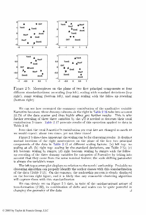
���� PRE�PROCESSING AND STANDARDIZING MIXED DATA ��
−5 0 5−2
−1
0
1
2 OliT
DomS
GreE
TomS
HucF
YanA
WarP AnnK
−2 −1 0 1 2
−2
−1
0
1
OliT DomS
GreE
TomS
HucF YanA WarP
AnnK
−1 −0.5 0 0.5 1−1
−0.5
0
0.5
1
OliT
DomS
GreE
TomS
HucF YanA
WarP
AnnK
−1 −0.5 0 0.5 1−1
−0.5
0
0.5
1
OliT
DomS
GreE
TomS HucF
YanA
WarP
AnnK
Figure ���� Masterpieces on the plane of two �rst principal components at fourdi�erent standardizations� no scaling �top left scaling with standard deviations �topright range scaling �bottom left and range scaling with the follow�up rescaling�bottom right �
We can see how overrated the summary contribution of the qualitative variableNarrative becomes� three dummy columns on the right in Table ���� take into account����� of the data scatter and thus highly a�ect any further results� This is whyfurther rescaling of these three variables by the
p� is needed to decrease their total
contribution � times� Table ���� presents results of this operation applied to data inTable �����
Note that the total Narrative�s contribution per cent has not changed as much aswe would expect� about two times yet not three times�
Figure ��� shows how important the scaling can be for clustering results� It displaysmutual locations of the eight masterpieces on the plane of the �rst two principalcomponents of the data in Table ���� at di�erent scaling factors� �a left top� noscaling at all� �b right top� scaling by the standard deviations see Table ����� �c left bottom� scaling by ranges� �d right bottom� scaling by ranges with the follow�up rescaling of the three dummy variables for categories of Narrative by taking intoaccount that they come from the same nominal feature� the scale shifting parameteris always the variable�s mean�
The left top scatter�plot displays no relation to the novels� authorship� Probably noclustering algorithm can properly identify the author classes with this standardizationof the data �Table ���� � On the contrary the authorship pattern is clearly displayedon the bottom right �gure and it is likely that any reasonable clustering algorithmwill capture them with this standardization�
We can clearly see on Figure ��� that in spite of the unidimensional nature oftransformation ����� its combination of shifts and scales can be quite powerful inchanging the geometry of the data� �
© 2005 by Taylor & Francis Group, LLC
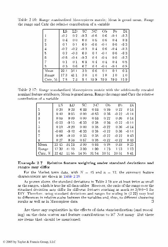
�� WHAT IS DATA
Table ����� Range standardized Masterpieces matrix� Mean is grand mean Rangethe range and Cntr the relative contribution of a variable�
LS LD SC NC Ob Pe Di� ��� �� ��� ��� �� ��� ���� �� � � ��� �� ��� ���� �� �� � ��� ��� �� ���� ��� ��� ��� �� �� ��� ���� �� ��� � �� ��� �� ���� ��� ��� ��� �� ��� �� ���� �� ��� �� �� ��� ��� ��� �� �� �� �� ��� ��� ��
Mean ���� ���� �� �� �� �� ��Range ���� ���� �� �� �� �� ��Cntr � ��� ��� ��� ���� ���� ���� ����
Table ����� Range standardized Masterpieces matrix with the additionally rescalednominal feature attributes� Mean is grand mean Range the range and Cntr the relativecontribution of a variable�
LS LD SC NC Ob Pe Di� ��� ��� ���� ���� ��� ���� ����� �� �� � ���� ��� ���� ����� �� �� � ���� ���� ��� ����� ���� ���� ���� ��� ��� ���� ����� ��� ���� � ��� ���� ��� ����� ��� ���� ���� ��� ���� ��� ����� �� ��� ��� ��� ���� ���� ���� ��� ��� ��� ��� ���� ���� ���
Mean ����� ����� �� ��� ��� ��� ���Range ���� ���� �� �� ���� ���� ����Cntr � ����� ����� ����� ����� ���� ���� ����
Example ���� Relative feature weighting under standard deviations andranges may di�er
For the Market town data with N � �� and n � �� the summary featurecharacteristics are shown in Table �����
As proven above the standard deviations in Table ���� are at least twice as smallas the ranges which is true for all data tables� However the ratio of the range over thestandard deviation may di�er for di�erent features reaching as much as ������ forDIY� Therefore using standard deviations and ranges for scaling in ����� may leadto di�erences in relative scales between the variables and thus to di�erent clusteringresults as well as in Masterpiece data� �
Are there any regularities in the e ects of data standardization �and rescaling� on the data scatter and feature contributions to it� Not many� But thereare items that should be mentioned�
© 2005 by Taylor & Francis Group, LLC

���� PRE�PROCESSING AND STANDARDIZING MIXED DATA ��
Table ����� Summary characteristics of the Market town data� Mean is grand meanStd the standard deviation Range the range and Cntr the relative contribution of avariable�
P PS Do Ho Ba Su Pe DIY SP PO CAB FMMean ����� ��� �� �� �� �� ��� ��� ��� ��� ��� ���Std ����� ��� ��� ��� � ��� ��� ��� ��� ��� ��� ��Range ������� ���� �� ��� ��� ��� ��� ��� ��� ��� ��� ���Cntr� � ��� �� ���� ��� ��� ��� ��� �� ���� ��� �� ����
Eect of shifting to the average� With shifting to the averages� the featurecontributions and variances become proportional to each other� Tv � Ns�v�for all v � V �
Eects of scaling of categories� Let us take a look at the e ect of scalingand rescaling coe�cients on categories� The contribution of a binaryattribute v� standardized according to ������� becomes Tv � Npv�� �pv���bv�
� where pv is the relative frequency of category v� This can beeither pv�� � pv� or � or � � pv depending on whether bv � � �range�or bv �
ppv��� pv� �Bernoulli standard deviation� or bv �
ppv �Pois
son standard deviation�� respectively� These can give some guidance inrescaling of binary categories� the rst option should be taken when bothzeros and ones are equally important� the second when the distributiondoes not matter and the third when it is only unities that matter�
Identity of binary and two�category features� An important issue facedby the user is how to treat a categorical feature with two categories such asgender �Male�Female� or voting �Democrat�Republican� or belongingnessto a group �Yes�No�� The threestep procedure of standardization makesthe issue irrelevant� there is no di erence between a twocategory featureand either of its binary representations�
Indeed� let x be a twocategory feature assigning each entity i � I witha category �eks�� or �eks�� whose relative frequencies are p� and p� suchthat p�!p� � �� Denote by y� a binary feature corresponding to category�eks�� so that y�i � � if xi � eks� and y�i � � if xi � eks�� Analogouslydene a binary feature y� corresponding to category �eks��� Obviously�y� and y� complement each other so that their sum makes an all unityvector�
In the rst stage of the standardization procedure� the user decideswhether x is to be converted to a binary feature or left as a categoricalone� In the former case� x is converted to a dummy feature� say� columny�� and in the latter case� x is converted into a twocolumn submatrix
© 2005 by Taylor & Francis Group, LLC
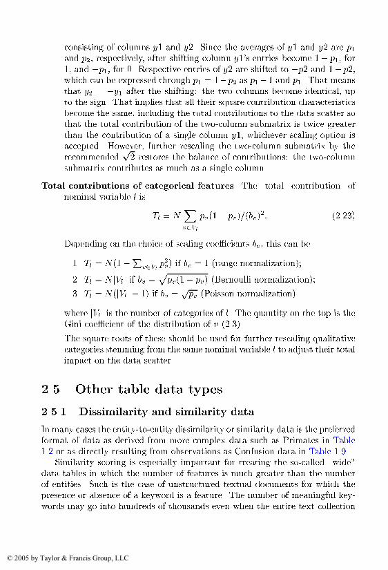
�� WHAT IS DATA
consisting of columns y� and y�� Since the averages of y� and y� are p�and p�� respectively� after shifting column y��s entries become �� p�� for�� and �p�� for �� Respective entries of y� are shifted to �p� and �� p��which can be expressed through p� � ��p� as p��� and p�� That meansthat y� � �y� after the shifting� the two columns become identical� upto the sign� That implies that all their square contribution characteristicsbecome the same� including the total contributions to the data scatter sothat the total contribution of the twocolumn submatrix is twice greaterthan the contribution of a single column y�� whichever scaling option isaccepted� However� further rescaling the twocolumn submatrix by therecommended
p� restores the balance of contributions� the twocolumn
submatrix contributes as much as a single column�
Total contributions of categorical features� The total contribution ofnominal variable l is
Tl � NXv�Vl
pv��� pv���bv��� ������
Depending on the choice of scaling coe�cients bv� this can be
�� Tl � N���Pv�Vlp�v� if bv � � �range normalization��
�� Tl � N jVlj if bv �ppv��� pv� �Bernoulli normalization��
�� Tl � N�jVlj � �� if bv � ppv �Poisson normalization��where jVlj is the number of categories of l� The quantity on the top is theGini coe�cient of the distribution of v ������
The square roots of these should be used for further rescaling qualitativecategories stemming from the same nominal variable l to adjust their totalimpact on the data scatter�
��� Other table data types
����� Dissimilarity and similarity data
In many cases the entitytoentity dissimilarity or similarity data is the preferredformat of data as derived from more complex data such as Primates in Table��� or as directly resulting from observations as Confusion data in Table ����Similarity scoring is especially important for treating the socalled �wide�
data tables in which the number of features is much greater than the numberof entities� Such is the case of unstructured textual documents for which thepresence or absence of a keyword is a feature� The number of meaningful keywords may go into hundreds of thousands even when the entire text collection
© 2005 by Taylor & Francis Group, LLC
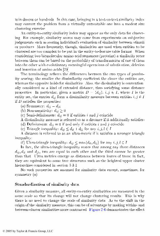
���� OTHER TABLE DATA TYPES ��
is in dozens or hundreds� In this case� bringing in a texttotext similarity indexmay convert the problem from a virtually untreatable one into a modest sizeclustering exercise�An entitytoentity similarity index may appear as the only data for cluster
ing� For example� similarity scores may come from experiments on subjectivejudgements such as scoring individual�s evaluation of similarity between stimulior products� More frequently� though� similarities are used when entities to beclustered are too complex to be put in the entitytofeature table format� Whenconsidering two biomolecular amino acid sequences �proteins� a similarity scorebetween them can be based on the probability of transformation of one of theminto the other with evolutionary meaningful operations of substitution� deletionand insertion of amino acids �����The terminology re�ects the di erences between the two types of proxim
ity scoring� the smaller the dissimilarity coe�cient the closer the entities are�whereas the opposite holds for similarities� Also� the dissimilarity is conventionally considered as a kind of extended distance� thus satisfying some distanceproperties� In particular� given a matrix D � �dij�� i� j � I � where I is theentity set� the entries dij form a dissimilarity measure between entities i� j � Iif D satises the properties��a� Symmetry� dij � dji��b� Nonnegativity� dij � ���c� Semideniteness� dij � � if entities i and j coincide�A dissimilarity measure is referred to as a distance if it additionally satises��d� Deniteness� dij � � if and only if entities i and j coincide��e� Triangle inequality� dij � dil ! dlj for any i� j� l � I �A distance is referred to as an ultrametric if it satises a stronger triangle
inequality��f� Ultratriangle inequality� dij � max�dil� dlj� for any i� j� l � I �In fact� the ultratriangle inequality states that among any three distances
dij � dil and djl� two are equal to each other and the third cannot be greaterthan that� Ultrametrics emerge as distances between leaves of trees� in fact�they are equivalent to some tree structures such as the heighted upper clusterhierarchies considered in section ������No such properties are assumed for similarity data except� sometimes� for
symmetry �a��
Standardization of similarity data
Given a similarity measure� all entitytoentity similarities are measured in thesame scale so that its change will not change clustering results� This is whythere is no need to change the scale of similarity data� As to the shift in theorigin of the similarity measure� this can be of advantage by making within andbetweencluster similarities more contrasted� Figure ��� demonstrates the e ect
© 2005 by Taylor & Francis Group, LLC
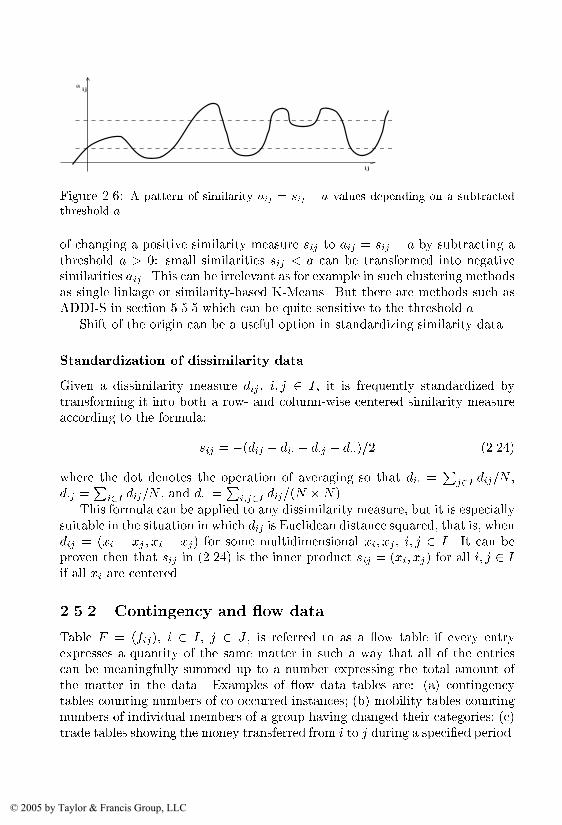
�� WHAT IS DATA
ij
aij
Figure ���� A pattern of similarity aij � sij � a values depending on a subtractedthreshold a�
of changing a positive similarity measure sij to aij � sij � a by subtracting athreshold a � �� small similarities sij � a can be transformed into negativesimilarities aij � This can be irrelevant as for example in such clustering methodsas single linkage or similaritybased KMeans� But there are methods such asADDIS in section ����� which can be quite sensitive to the threshold a�Shift of the origin can be a useful option in standardizing similarity data�
Standardization of dissimilarity data
Given a dissimilarity measure dij � i� j � I � it is frequently standardized bytransforming it into both a row and columnwise centered similarity measureaccording to the formula�
sij � ��dij � di� � d�j � d����� ������
where the dot denotes the operation of averaging so that di� �P
j�I dij�N �d�j �
Pi�I dij�N � and d�� �
Pi�j�I dij��N N��
This formula can be applied to any dissimilarity measure� but it is especiallysuitable in the situation in which dij is Euclidean distance squared� that is� whendij � �xi � xj � xi � xj� for some multidimensional xi� xj � i� j � I � It can beproven then that sij in ������ is the inner product sij � �xi� xj� for all i� j � Iif all xi are centered�
����� Contingency and �ow data
Table F � �fij�� i � I � j � J � is referred to as a �ow table if every entryexpresses a quantity of the same matter in such a way that all of the entriescan be meaningfully summed up to a number expressing the total amount ofthe matter in the data� Examples of �ow data tables are� �a� contingencytables counting numbers of cooccurred instances� �b� mobility tables countingnumbers of individual members of a group having changed their categories� �c�trade tables showing the money transferred from i to j during a specied period�
© 2005 by Taylor & Francis Group, LLC

���� OTHER TABLE DATA TYPES ��
This type of data is of particular interest in processing massive informationsources� The data itself can be untreatable within timememory constraints�but by counting cooccurrences of categories of interest in a sample it can bepreprocessed into the �ow data format and analyzed as such�
The nature of the data associates weights of row categories i � I � fi� �Pj�J fij � and column categories j � J � f�j �
Pi�I fij � the total �ow from
i and that to j� The total �ow volume is f�� �P
i�I
Pj�J fij � which is the
summary weight� f�� �P
j�J f�j �P
i�I fi�� Extending concepts introducedin section ����� for contingency tables to the general �ow data� we can extendthe denition of the relative Quetelet index as
qij �fijf��fi�f�j
� � ������
This index� in fact� compares the share of j in i�s transaction� p�j�i� � fij�fi��with the share of j in the overall �ow� p�j� � f�j�f���
Indeed� it is easy to see that qij is the relative di erence of the two� qij ��p�j�i�� p�j���p�j�� Obviously� qij � � when there is no di erence�
Transformation ������ is a standardization of �ow data which takes intoaccount the data�s nature� Standardization ������ is very close to the socallednormalization of Rao and Sabovala widely used in marketing research and� also�the �marginal� crossproduct ratio utilized in the analysis of contingency data�Both can be expressed as pij transformed into qij ! ��
Example ���� Quetelet coe�cients for Confusion data Coe�cients ����� arepresented in Table ����� One can see from the table that the numerals overwhelminglyrespond to themselves� However there are also a few positive entries in the tableoutside of the diagonal� For instance � is perceived as � with the frequency �����greater than the average and � is perceived as � and vice versa with also higherfrequencies than the average� �
Table ����� Relative Quetelet coe�cients for Confusion data per cent�
Sti� Responsemulus � � � � � � � �� ����� ���� ���� ����� ���� ����� ����� ������ ��� � ���� ���� ���� ����� ���� ����� ���� ���� ���� ��� � ���� ���� ���� ����� ���� ���� ������ ���� ���� ��� � ���� �� ����� ���� ���� ���� ����� ���� ���� ����� � ������ ���� ����� ����� ���� ����� ����� ���� ���� ���� � ����� ����� ����� ���� ����� �� ����� ���� ��� ����� � ����� ��� ���� ����� ����� ���� ������ ����� ������ ��� � ���� ���� ���� ����� ���� ���� ����� ����� ����� ���� ���� ����� ���� ���� ���� ����� ����� ����� ���� ��� � ����� ���� ���� ���� ����� ���� ���� ����� ����� ����� �����
© 2005 by Taylor & Francis Group, LLC
�� WHAT IS DATA
Taking into account that the �ow data entries can be meaningfully summedup to the total �ow volume� the distance between row entities in a contingencytable is dened by weighting the columns by their �masses� p�l as follows�
��k� k�� �Xj�J
p�j�qkj � qk�j��� ������
This is equal to the socalled chisquare distance dened between row conditional proles in the Correspondence factor analysis �see section ������� Theformula ������ is similar to formula ������ for Euclidean distance squared exceptfor the weights� A similar chisquare distance can be dened for columns�The concept of data scatter for contingency data is also introduced with
weighting�
X��P � �XI�I
Xj�J
pi�p�jq�ij ������
The notation re�ects the fact that this value is closely connected with thePearson chisquare contingency coe�cient� dened in ������ above �thus to Q�
������ as well�� Elementary algebraic manipulations show that X��P � � X��Note that in this context the chisquared coe�cient has nothing to do with thestatistical independence� it is just a weighted data scatter measure compatiblewith the specic properties of �ow and contingency data� In particular� it is notdi�cult to prove an analogue to a property of the conventional data scatter�X��P � is the sum of chisquare distances ��k� �� over all k�Thus� Pearson�s chisquared coe�cient here emerges as the data scatter
after the data have been standardized into Quetelet coe�cients� For Table ���transformed here into Table ���� the coe�cient is equal to ���� which is �� of �� the maximum value of the coe�cient for �� �� tables�
© 2005 by Taylor & Francis Group, LLC
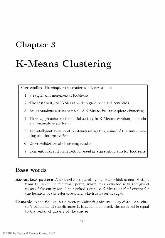
Chapter �
K�Means Clustering
After reading this chapter the reader will know about�
�� Straight and incremental KMeans�
�� The instability of KMeans with regard to initial centroids�
�� An anomalous cluster version of KMeans for incomplete clustering�
�� Three approaches to the initial setting in KMeans� random� maxminand anomalous pattern�
�� An intelligent version of KMeans mitigating issues of the initial setting and interpretation�
�� Crossvalidation of clustering results�
�� Conventional and contribution based interpretation aids for KMeans�
Base words
Anomalous pattern A method for separating a cluster which is most distantfrom the socalled reference point� which may coincide with the grandmean of the entity set� The method works as KMeans at K�� except forthe location of the reference point which is never changed�
Centroid Amultidimensional vector minimizing the summary distance to cluster�s elements� If the distance is Euclidean squared� the centroid is equalto the center of gravity of the cluster�
��
© 2005 by Taylor & Francis Group, LLC
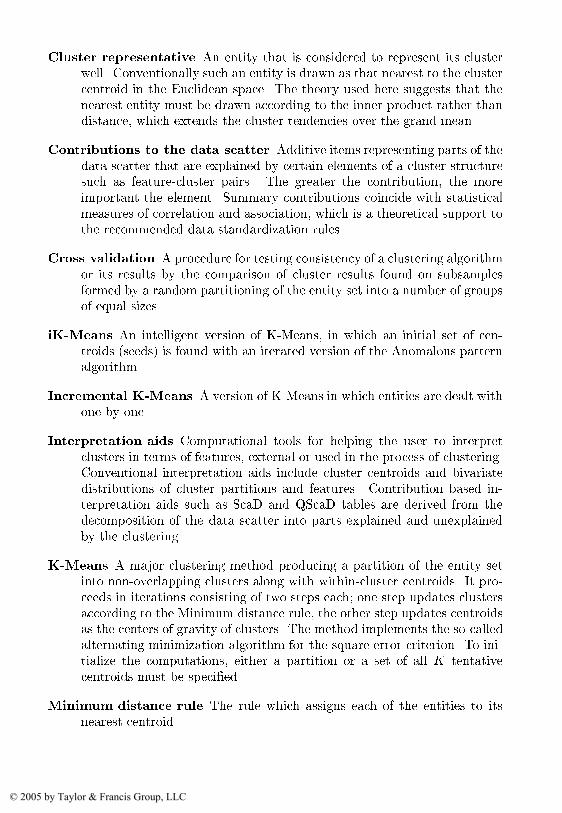
�� K�MEANS CLUSTERING
Cluster representative An entity that is considered to represent its clusterwell� Conventionally such an entity is drawn as that nearest to the clustercentroid in the Euclidean space� The theory used here suggests that thenearest entity must be drawn according to the inner product rather thandistance� which extends the cluster tendencies over the grand mean�
Contributions to the data scatter Additive items representing parts of thedata scatter that are explained by certain elements of a cluster structuresuch as featurecluster pairs� The greater the contribution� the moreimportant the element� Summary contributions coincide with statisticalmeasures of correlation and association� which is a theoretical support tothe recommended data standardization rules�
Cross validation A procedure for testing consistency of a clustering algorithmor its results by the comparison of cluster results found on subsamplesformed by a random partitioning of the entity set into a number of groupsof equal sizes�
iK�Means An intelligent version of KMeans� in which an initial set of centroids �seeds� is found with an iterated version of the Anomalous patternalgorithm�
Incremental K�Means A version of KMeans in which entities are dealt withonebyone�
Interpretation aids Computational tools for helping the user to interpretclusters in terms of features� external or used in the process of clustering�Conventional interpretation aids include cluster centroids and bivariatedistributions of cluster partitions and features� Contribution based interpretation aids such as ScaD and QScaD tables are derived from thedecomposition of the data scatter into parts explained and unexplainedby the clustering�
K�Means A major clustering method producing a partition of the entity setinto nonoverlapping clusters along with withincluster centroids� It proceeds in iterations consisting of two steps each� one step updates clustersaccording to the Minimum distance rule� the other step updates centroidsas the centers of gravity of clusters� The method implements the socalledalternating minimization algorithm for the square error criterion� To initialize the computations� either a partition or a set of all K tentativecentroids must be specied�
Minimum distance rule The rule which assigns each of the entities to itsnearest centroid�
© 2005 by Taylor & Francis Group, LLC
BASE WORDS ��
Reference point A vector in the variable space serving as the space origin�The Anomalous pattern is sought starting from an entity which is thefarthest from the reference point� which thus models the norm from whichthe Anomalous pattern deviates most�
ScaD and QScaD tables Interpretation aids helping to capture clusterspecic features that are relevant to KMeans clustering results� ScaD is aclustertofeature table whose entries are clustertofeature contributionsto the data scatter� QScaD is a table of the relative Quitelet coe�cientsof the ScaD entries to express how much they di er from the average�
Square error criterion The sum of summary distances from cluster elementsto the cluster centroids� which is minimized by KMeans� The distanceused is the Euclidean distance squared� which is compatible with theleastsquares data recovery criterion�
© 2005 by Taylor & Francis Group, LLC
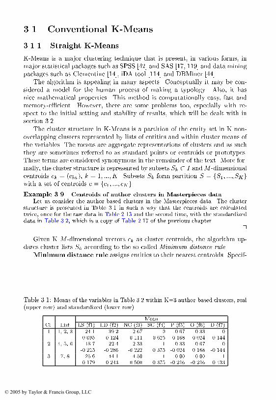
�� K�MEANS CLUSTERING
��� Conventional K�Means
����� Straight KMeans
KMeans is a major clustering technique that is present� in various forms� inmajor statistical packages such as SPSS ���� and SAS ���� ���� and data miningpackages such as Clementine ����� iDA tool ����� and DBMiner �����The algorithm is appealing in many aspects� Conceptually it may be con
sidered a model for the human process of making a typology� Also� it hasnice mathematical properties� This method is computationally easy� fast andmemorye�cient� However� there are some problems too� especially with respect to the initial setting and stability of results� which will be dealt with insection ����The cluster structure in KMeans is a partition of the entity set in K non
overlapping clusters represented by lists of entities and within cluster means ofthe variables� The means are aggregate representations of clusters and as suchthey are sometimes referred to as standard points or centroids or prototypes�These terms are considered synonymous in the remainder of the text� More formally� the cluster structure is represented by subsets Sk � I andM dimensionalcentroids ck � �ckv�� k � �� ����K� Subsets Sk form partition S � fS�� ���� SKgwith a set of centroids c � fc�� ���� cKg�Example ���� Centroids of author clusters in Masterpieces data
Let us consider the author�based clusters in the Masterpieces data� The clusterstructure is presented in Table ��� in such a way that the centroids are calculatedtwice once for the raw data in Table ���� and the second time with the standardizeddata in Table ��� which is a copy of Table ���� of the previous chapter�
�
Given K M dimensional vectors ck as cluster centroids� the algorithm updates cluster lists Sk according to the socalled Minimum distance rule�
Minimum distance rule assigns entities to their nearest centroids� Specif
Table ���� Means of the variables in Table ��� within K�� author�based clusters real�upper row and standardized �lower row �
MeanCl� List LS �f� LD �f� NC �f� SC �f P �f� O �f� D �f� � �� �� � ��� ��� ���� � ���� ���� �
���� ���� ������ ������ ����� ����� ����� � �� � ���� ��� ���� � ���� ���� �
������ ������ ������ ����� ����� ����� ����� �� � ���� �� ��� � ���� ���� �
���� ���� ����� ����� ������ ������ ����
© 2005 by Taylor & Francis Group, LLC
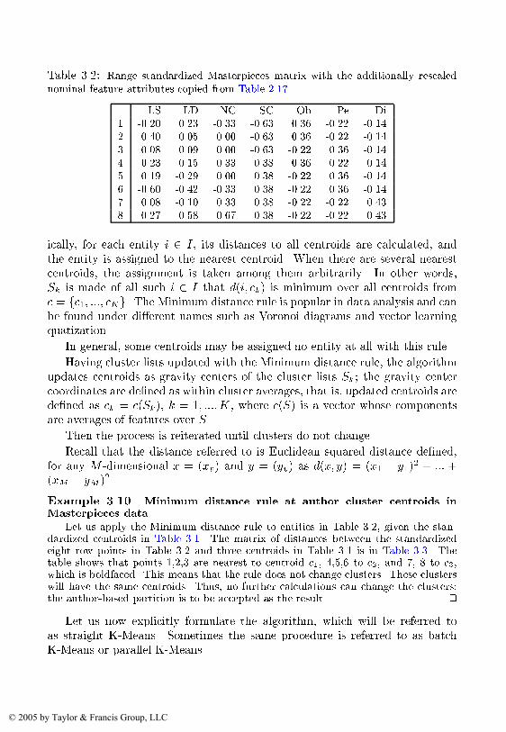
���� CONVENTIONAL K�MEANS ��
Table ���� Range standardized Masterpieces matrix with the additionally rescalednominal feature attributes copied from Table �����
LS LD NC SC Ob Pe Di� ��� ��� ���� ���� ��� ���� ����� �� �� � ���� ��� ���� ����� �� �� � ���� ���� ��� ����� ���� ���� ���� ��� ��� ���� ����� ��� ���� � ��� ���� ��� ����� ��� ���� ���� ��� ���� ��� ����� �� ��� ��� ��� ���� ���� ���� ��� ��� ��� ��� ���� ���� ���
ically� for each entity i � I � its distances to all centroids are calculated� andthe entity is assigned to the nearest centroid� When there are several nearestcentroids� the assignment is taken among them arbitrarily� In other words�Sk is made of all such i � I that d�i� ck� is minimum over all centroids fromc � fc�� ���� cKg� The Minimum distance rule is popular in data analysis and canbe found under di erent names such as Voronoi diagrams and vector learningquatization�
In general� some centroids may be assigned no entity at all with this rule�
Having cluster lists updated with the Minimum distance rule� the algorithmupdates centroids as gravity centers of the cluster lists Sk� the gravity centercoordinates are dened as within cluster averages� that is� updated centroids aredened as ck � c�Sk�� k � �� ����K� where c�S� is a vector whose componentsare averages of features over S�
Then the process is reiterated until clusters do not change�
Recall that the distance referred to is Euclidean squared distance dened�for any M dimensional x � �xv� and y � �yv� as d�x� y� � �x� � y��
� ! ��� !�xM � yM �
��
Example ���� Minimum distance rule at author cluster centroids inMasterpieces data
Let us apply the Minimum distance rule to entities in Table ��� given the stan�dardized centroids in Table ���� The matrix of distances between the standardizedeight row points in Table ��� and three centroids in Table ��� is in Table ���� Thetable shows that points ��� are nearest to centroid c� ��� to c� and � � to c�which is boldfaced� This means that the rule does not change clusters� These clusterswill have the same centroids� Thus no further calculations can change the clusters�the author�based partition is to be accepted as the result� �
Let us now explicitly formulate the algorithm� which will be referred toas straight KMeans� Sometimes the same procedure is referred to as batchKMeans or parallel KMeans�
© 2005 by Taylor & Francis Group, LLC
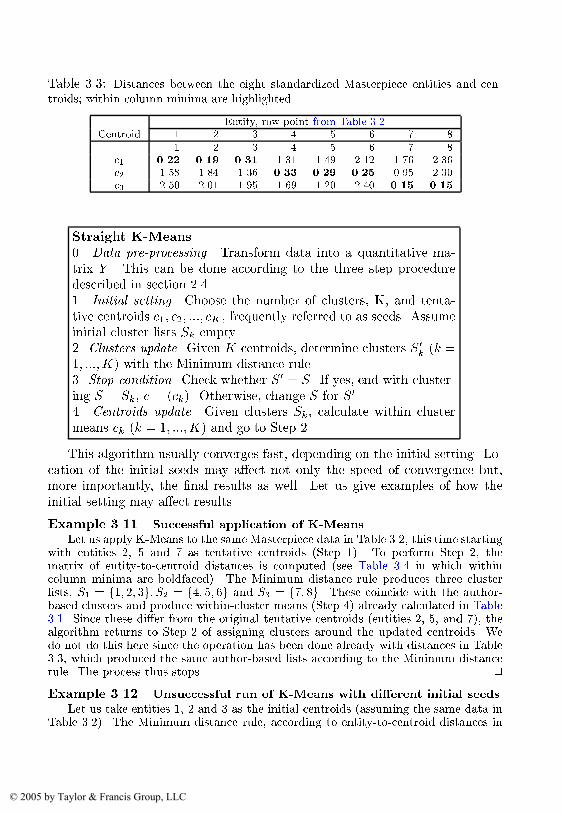
�� K�MEANS CLUSTERING
Table ���� Distances between the eight standardized Masterpiece entities and cen�troids� within column minima are highlighted�
Entity� row point from Table ���Centroid � � � � � � �
� � � � � � �c� ���� ���� ���� ���� �� ���� ���� ����c� ���� ��� ���� ���� ���� ���� ��� ����c� ���� ���� ��� ��� ���� ��� ���� ����
Straight K�Means�� Data pre�processing� Transform data into a quantitative matrix Y � This can be done according to the three step proceduredescribed in section ������ Initial setting� Choose the number of clusters� K� and tentative centroids c�� c�� ���� cK � frequently referred to as seeds� Assumeinitial cluster lists Sk empty��� Clusters update� Given K centroids� determine clusters S�k �k ��� ����K� with the Minimum distance rule��� Stop�condition� Check whether S� � S� If yes� end with clustering S � Sk� c � �ck�� Otherwise� change S for S
���� Centroids update� Given clusters Sk� calculate within clustermeans ck �k � �� ����K� and go to Step ��
This algorithm usually converges fast� depending on the initial setting� Location of the initial seeds may a ect not only the speed of convergence but�more importantly� the nal results as well� Let us give examples of how theinitial setting may a ect results�
Example ����� Successful application of K Means
Let us apply K�Means to the same Masterpiece data in Table ��� this time startingwith entities � � and � as tentative centroids �Step � � To perform Step � thematrix of entity�to�centroid distances is computed �see Table ��� in which withincolumn minima are boldfaced � The Minimum distance rule produces three clusterlists S� � f�� �� �g� S� � f�� �� �g and S� � f�� �g� These coincide with the author�based clusters and produce within�cluster means �Step � already calculated in Table���� Since these di�er from the original tentative centroids �entities � � and � thealgorithm returns to Step � of assigning clusters around the updated centroids� Wedo not do this here since the operation has been done already with distances in Table��� which produced the same author�based lists according to the Minimum distancerule� The process thus stops� �
Example ����� Unsuccessful run of K Means with di�erent initial seeds
Let us take entities � � and � as the initial centroids �assuming the same data inTable ��� � The Minimum distance rule according to entity�to�centroid distances in
© 2005 by Taylor & Francis Group, LLC

���� CONVENTIONAL K�MEANS ��
Table ���� Distances between entities � � � as seeds and the standardized Master�piece entities�
Row�pointCentroid � � � � � � �
� ���� ���� ���� ���� ���� �� ��� ���� ���� ���� ���� ���� ���� ���� ���� ����� ���� ��� ���� ���� ���� ���� ���� ���
Table ���� Distances between the standardized Masterpiece entities and entities � �� as seeds�
Row�pointCentroid � � � � � � �
� ���� ���� ���� ���� ���� ���� ���� ����� ���� ���� ���� ���� ���� �� ��� ���� ���� ���� ���� �� ��� ��� ��� ���
Table ��� leads to cluster lists S� � f�� �g� S� � f�g and S� � f�� �� �� �� �g� Withthe centroids updated at Step � as means of these clusters a new application of Step� leads to slightly changed cluster lists S� � f�� �� �g� S� � f�g and S� � f�� �� �� �g�Their means calculated it is not di�cult to see that the Minimum distance rule doesnot change clusters anymore� Thus the lists represent the �nal outcome which di�ersfrom the author�based solution�
�
The intuitive inappropriateness of the results in this example may be explained by the stupid choice of the initial centroids� all by the same author�However� KMeans can lead to inconvenient results even if the initial setting isselected according to clustering by authors�
Table ���� Distances between the standardized Masterpiece entities and entities � �� as tentative centroids�
Row�pointCentroid � � � � � � �
� ���� ���� �� ���� ���� ���� ���� ���� ���� ���� �� ���� ��� ��� ���� ���� ���� ��� ���� ���� ��� ���� ���� ���
Example ����� Unsuccessful K Means with author based initial seeds
With the initial centroids at rows � � and � the entity�to�centroid matrix inTable ��� leads to cluster lists S� � f�� �� �g� S� � f�� �g and S� � f�� �� �g that donot change in the follow�up operations� These results put a piece by Mark Twainamong those by Leo Tolstoy� Not a good outcome� �
© 2005 by Taylor & Francis Group, LLC
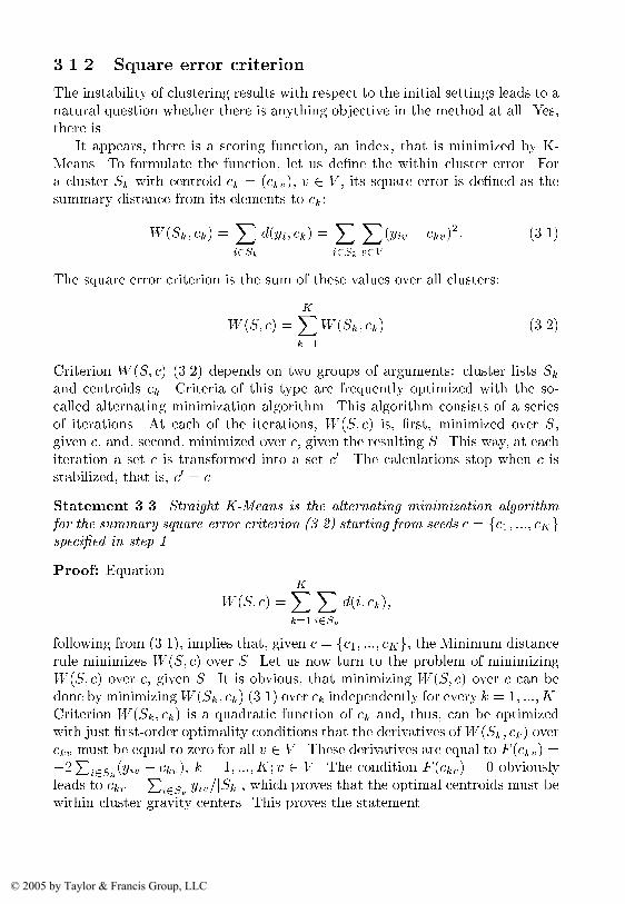
�� K�MEANS CLUSTERING
����� Square error criterion
The instability of clustering results with respect to the initial settings leads to anatural question whether there is anything objective in the method at all� Yes�there is�It appears� there is a scoring function� an index� that is minimized by K
Means� To formulate the function� let us dene the within cluster error� Fora cluster Sk with centroid ck � �ckv�� v � V � its square error is dened as thesummary distance from its elements to ck�
W �Sk� ck� �Xi�Sk
d�yi� ck� �Xi�Sk
Xv�V
�yiv � ckv��� �����
The square error criterion is the sum of these values over all clusters�
W �S� c� �
KXk��
W �Sk� ck� �����
Criterion W �S� c� ����� depends on two groups of arguments� cluster lists Skand centroids ck� Criteria of this type are frequently optimized with the socalled alternating minimization algorithm� This algorithm consists of a seriesof iterations� At each of the iterations� W �S� c� is� rst� minimized over S�given c� and� second� minimized over c� given the resulting S� This way� at eachiteration a set c is transformed into a set c�� The calculations stop when c isstabilized� that is� c� � c�
Statement ���� Straight K�Means is the alternating minimization algorithmfor the summary square�error criterion ���� starting from seeds c � fc�� ���� cKgspeci�ed in step �
Proof� Equation
W �S� c� �
KXk��
Xi�Sk
d�i� ck��
following from ������ implies that� given c � fc�� ���� cKg� the Minimum distancerule minimizes W �S� c� over S� Let us now turn to the problem of minimizingW �S� c� over c� given S� It is obvious� that minimizing W �S� c� over c can bedone by minimizingW �Sk� ck� ����� over ck independently for every k � �� ����K�Criterion W �Sk� ck� is a quadratic function of ck and� thus� can be optimizedwith just rstorder optimality conditions that the derivatives ofW �Sk� ck� overckv must be equal to zero for all v � V � These derivatives are equal to F �ckv� ���Pi�Sk
�yiv � ckv�� k � �� ����K� v � V � The condition F �ckv� � � obviouslyleads to ckv �
Pi�Sk
yiv�jSkj� which proves that the optimal centroids must bewithin cluster gravity centers� This proves the statement�
© 2005 by Taylor & Francis Group, LLC
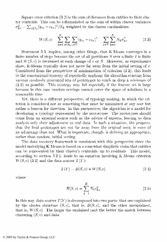
���� CONVENTIONAL K�MEANS ��
Squareerror criterion ����� is the sum of distances from entities to their cluster centroids� This can be reformulated as the sum of within cluster variances �kv �
Pi�Sk
�yiv � ckv���Nk weighted by the cluster cardinalities�
W �S� c� �
KXk��
Xi�Sk
Xv�V
�yiv � ckv�� �
Xv�V
KXk��
Nk �kv �����
Statement ���� implies� among other things� that KMeans converges in anite number of steps because the set of all partitions S over a nite I is niteand W �S� c� is decreased at each change of c or S� Moreover� as experimentsshow� KMeans typically does not move far away from the initial setting of c�Considered from the perspective of minimization of criterion ������ this leadsto the conventional strategy of repeatedly applying the algorithm starting fromvarious randomly generated sets of prototypes to reach as deep a minimum of����� as possible� This strategy may fail especially if the feature set is largebecause in this case random settings cannot cover the space of solutions in areasonable time�Yet� there is a di erent perspective� of typology making� in which the cri
terion is considered not as something that must be minimized at any cost butrather a beacon for direction� In this perspective� the algorithm is a model fordeveloping a typology represented by the prototypes� The prototypes shouldcome from an external source such as the advice of experts� leaving to dataanalysis only their adjustment to real data� In such a situation� the propertythat the nal prototypes are not far away from the original ones� is more ofan advantage than not� What is important� though� is dening an appropriate�rather than random� initial setting�The data recovery framework is consistent with this perspective since the
model underlying KMeans is based on a somewhat simplistic claim that entitiescan be represented by their cluster�s centroids� up to residuals� This model�according to section ������ leads to an equation involving KMeans criterionW �S� c� ����� and the data scatter T �Y ��
T �Y � � B�S� c� !W �S� c� �����
where
B�S� c� �
KXk��
Nkc�kv �����
In this way� data scatter T �Y � is decomposed into two parts� that one explainedby the cluster structure �S� c�� that is� B�S� c�� and the other unexplained�that is� W �S� c�� The larger the explained part the better the match betweenclustering �S� c� and data�
© 2005 by Taylor & Francis Group, LLC
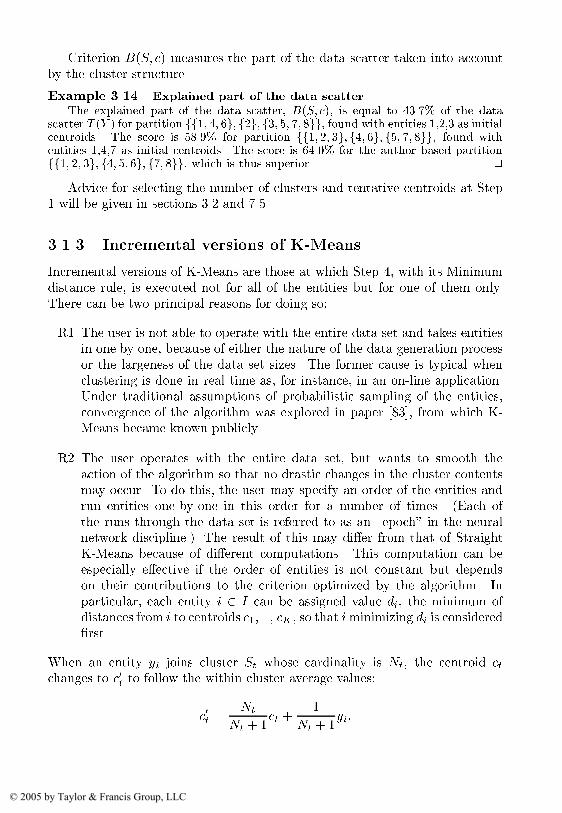
�� K�MEANS CLUSTERING
Criterion B�S� c� measures the part of the data scatter taken into accountby the cluster structure�
Example ����� Explained part of the data scatter
The explained part of the data scatter B�S� c is equal to ����� of the datascatter T �Y for partition ff�� �� �g� f�g� f�� �� �� �gg found with entities ��� as initialcentroids� The score is ����� for partition ff�� �� �g� f�� �g� f�� �� �gg found withentities ��� as initial centroids� The score is ���� for the author based partitionff�� �� �g� f�� �� �g� f�� �gg which is thus superior� �
Advice for selecting the number of clusters and tentative centroids at Step� will be given in sections ��� and ����
����� Incremental versions of KMeans
Incremental versions of KMeans are those at which Step �� with its Minimumdistance rule� is executed not for all of the entities but for one of them only�There can be two principal reasons for doing so�
R� The user is not able to operate with the entire data set and takes entitiesin one by one� because of either the nature of the data generation processor the largeness of the data set sizes� The former cause is typical whenclustering is done in real time as� for instance� in an online application�Under traditional assumptions of probabilistic sampling of the entities�convergence of the algorithm was explored in paper ����� from which KMeans became known publicly�
R� The user operates with the entire data set� but wants to smooth theaction of the algorithm so that no drastic changes in the cluster contentsmay occur� To do this� the user may specify an order of the entities andrun entities onebyone in this order for a number of times� �Each ofthe runs through the data set is referred to as an �epoch� in the neuralnetwork discipline�� The result of this may di er from that of StraightKMeans because of di erent computations� This computation can beespecially e ective if the order of entities is not constant but dependson their contributions to the criterion optimized by the algorithm� Inparticular� each entity i � I can be assigned value di� the minimum ofdistances from i to centroids c������ cK � so that iminimizing di is consideredrst�
When an entity yi joins cluster St whose cardinality is Nt� the centroid ctchanges to c�t to follow the within cluster average values�
c�t �Nt
Nt ! �ct !
�
Nt ! �yi�
© 2005 by Taylor & Francis Group, LLC
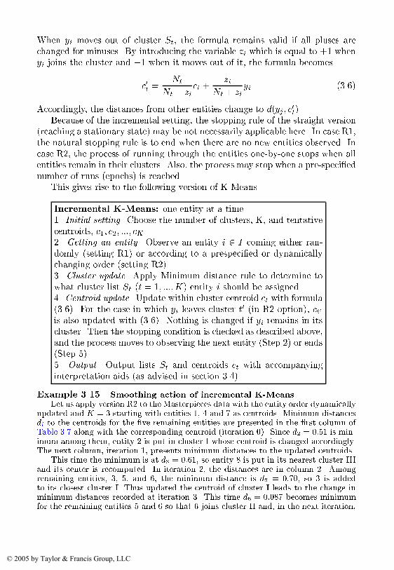
���� CONVENTIONAL K�MEANS ��
When yi moves out of cluster St� the formula remains valid if all pluses arechanged for minuses� By introducing the variable zi which is equal to !� whenyi joins the cluster and �� when it moves out of it� the formula becomes
c�t �Nt
Nt ! zict !
ziNt ! zi
yi �����
Accordingly� the distances from other entities change to d�yj � c�t��
Because of the incremental setting� the stopping rule of the straight version�reaching a stationary state� may be not necessarily applicable here� In case R��the natural stopping rule is to end when there are no new entities observed� Incase R�� the process of running through the entities onebyone stops when allentities remain in their clusters� Also� the process may stop when a prespeciednumber of runs �epochs� is reached�This gives rise to the following version of KMeans�
Incremental K�Means� one entity at a time��� Initial setting� Choose the number of clusters� K� and tentativecentroids� c�� c�� ���� cK ��� Getting an entity� Observe an entity i � I coming either randomly �setting R�� or according to a prespecied or dynamicallychanging order �setting R����� Cluster update� Apply Minimum distance rule to determine towhat cluster list St �t � �� ����K� entity i should be assigned��� Centroid update� Update within cluster centroid ct with formula������ For the case in which yi leaves cluster t
� �in R� option�� ct�
is also updated with ������ Nothing is changed if yi remains in itscluster� Then the stopping condition is checked as described above�and the process moves to observing the next entity �Step �� or ends�Step ����� Output� Output lists St and centroids ct with accompanyinginterpretation aids �as advised in section �����
Example ����� Smoothing action of incremental K MeansLet us apply version R� to the Masterpieces data with the entity order dynamically
updated and K � � starting with entities � � and � as centroids� Minimum distancesdi to the centroids for the �ve remaining entities are presented in the �rst column ofTable ��� along with the corresponding centroid �iteration � Since d� � ��� is min�imum among them entity � is put in cluster I whose centroid is changed accordingly�The next column iteration � presents minimum distances to the updated centroids�
This time the minimum is at d� � ��� so entity � is put in its nearest cluster IIIand its center is recomputed� In iteration � the distances are in column �� Amongremaining entities � � and � the minimum distance is d� � �� so � is addedto its closest cluster I� Thus updated the centroid of cluster I leads to the change inminimum distances recorded at iteration �� This time d� � ��� becomes minimumfor the remaining entities � and � so that � joins cluster II and in the next iteration
© 2005 by Taylor & Francis Group, LLC
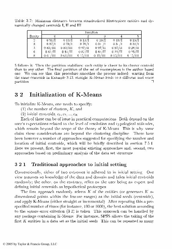
�� K�MEANS CLUSTERING
Table ���� Minimum distances between standardized Masterpiece entities and dy�namically changed centroids I II and III�
IterationEntity � � � � �
� �����I �����I �����I ����I ����I ����I� �����I �����I �����I ���� �I �����I �����I� �����III �����III ����II ����II ����II �����II� �����II �����II �����II �����II �����II �����II� �����III �����III �����III �����III �����III �����III
� follows it� Then the partition stabilizes� each entity is closer to its cluster centroidthan to any other� The �nal partition of the set of masterpieces is the author basedone� We can see that this procedure smoothes the process indeed� starting fromthe same centroids in Example ���� straight K�Means leads to a di�erent and worsepartition� �
��� Initialization of K�Means
To initialize KMeans� one needs to specify���� the number of clusters� K� and��� initial centroids� c�� c�� ���� cK �Each of these can be of issue in practical computations� Both depend on the
user�s expectations related to the level of resolution and typological attitudes�which remain beyond the scope of the theory of KMeans� This is why someclaim these considerations are beyond the clustering discipline� There havebeen however a number of approaches suggested for specifying the number andlocation of initial centroids� which will be brie�y described in section ������Here we present� rst� the most popular existing approaches and� second� twoapproaches based on preliminary analysis of the data set structure�
����� Traditional approaches to initial setting
Conventionally� either of two extremes is adhered to in initial setting� Oneview assumes no knowledge of the data and domain and takes initial centroidsrandomly� the other� on the contrary� relies on the user being an expert anddening initial centroids as hypothetical prototypes�The rst approach randomly selects K of the entities �or generates K n
dimensional points within the feature ranges� as the initial seeds �centroids��and apply KMeans �either straight or incremental�� After repeating this a prespecied number of times �for instance� ��� or ������ the best solution accordingto the squareerror criterion ����� is taken� This approach can be handled byany package containing KMeans� For instance� SPSS allows the taking of therst K entities in a data set as the initial seeds� This can be repeated as many
© 2005 by Taylor & Francis Group, LLC
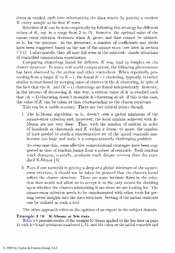
���� INITIALIZATION OF K�MEANS ��
times as needed� each time reformatting the data matrix by putting a randomK entity sample as its rst K rows�Selection ofK can be done empirically by following this strategy for di erent
values of K� say� in a range from � to ��� However� the optimal value of thesquareerror criterion decreases when K grows and thus cannot be utilized�as is� for the purpose� In the literature� a number of coe�cients and trickshave been suggested based on the use of the square error �see later in section������� Unfortunately� they all may fail even in the relatively simple situationsof controlled computation experiments�Comparing clusterings found for di erent K may lead to insights on the
cluster structure� In many real world computations� the following phenomenonhas been observed by the author and other researchers� When repeatedly proceeding from a largerK to K��� the found K�� clustering� typically� is rathersimilar to that found by merging some of clusters in the K clustering� in spite ofthe fact that the K and �K���clusterings are found independently� However�in the process of decreasing K this way� a critical value of K is reached suchthat �K � ��clustering doesn�t resemble Kclustering at all� If this is the case�the value of K can be taken as that corresponding to the cluster structure�This can be a viable strategy� There are two critical points though�
�� The KMeans algorithm� as is� doesn�t seek a global minimum of thesquareerror criterion and� moreover� the local minima achieved with KMeans are not very deep� Thus� with the number of entities in orderof hundreds or thousands and K within a dozen� or more� the numberof tries needed to reach a representative set of the initial centroids maybecome too large and make it a computationally challenging problem�
To overcome this� some e ective computational strategies have been suggested as that of random jumps from a subset of centroids� Such randomtrack changing� typically� produces much deeper minima than the standard KMeans �����
�� Even if one succeeds in getting a deep or a global minimum of the squareerror criterion� it should not be taken for granted that the clusters foundre�ect the cluster structure� There are some intrinsic �aws in the criterion that would not allow us to accept it as the only means for decidingupon whether the clusters minimizing it are those we are looking for� Thesquareerror criterion needs to be supplemented with other tools for getting better insights into the data structure� Setting of the initial centroidscan be utilized as such a tool�
The other approach relies on the opinion of an expert in the subject domain�
Example ����� K Means at Iris dataTable ��� presents results of the straight K�Means applied to the Iris data on page
�� with K�� and specimens numbered � �� and �� taken as the initial centroids and
© 2005 by Taylor & Francis Group, LLC
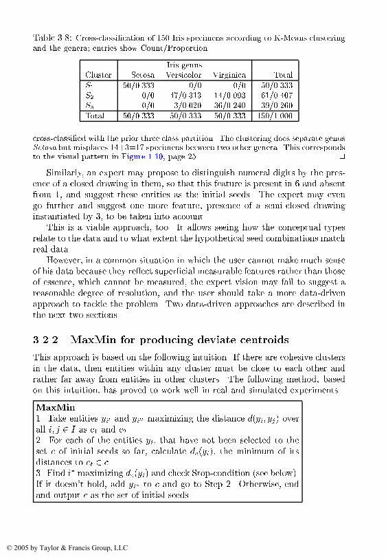
�� K�MEANS CLUSTERING
Table ���� Cross�classi�cation of �� Iris specimens according to K�Means clusteringand the genera� entries show Count�Proportion�
Iris genusCluster Setosa Versicolor Virginica Total
S� ������ � � ������S� � ������� ������ ������S� � ���� ������ ������
Total ������ ������ ������ �����
cross�classi�ed with the prior three class partition� The clustering does separate genusSetosa but misplaces ������� specimens between two other genera� This correspondsto the visual pattern in Figure ��� page ��� �
Similarly� an expert may propose to distinguish numeral digits by the presence of a closed drawing in them� so that this feature is present in � and absentfrom �� and suggest these entities as the initial seeds� The expert may evengo further and suggest one more feature� presence of a semiclosed drawinginstantiated by �� to be taken into account�This is a viable approach� too� It allows seeing how the conceptual types
relate to the data and to what extent the hypothetical seed combinations matchreal data�However� in a common situation in which the user cannot make much sense
of his data because they re�ect supercial measurable features rather than thoseof essence� which cannot be measured� the expert vision may fail to suggest areasonable degree of resolution� and the user should take a more datadrivenapproach to tackle the problem� Two datadriven approaches are described inthe next two sections�
����� MaxMin for producing deviate centroids
This approach is based on the following intuition� If there are cohesive clustersin the data� then entities within any cluster must be close to each other andrather far away from entities in other clusters� The following method� basedon this intuition� has proved to work well in real and simulated experiments�
MaxMin�� Take entities yi� and yi�� maximizing the distance d�yi� yj� overall i� j � I as c� and c���� For each of the entities yi� that have not been selected to theset c of initial seeds so far� calculate dc�yi�� the minimum of itsdistances to ct � c��� Find i� maximizing dc�yi� and check Stopcondition �see below��If it doesn�t hold� add yi� to c and go to Step �� Otherwise� endand output c as the set of initial seeds�
© 2005 by Taylor & Francis Group, LLC
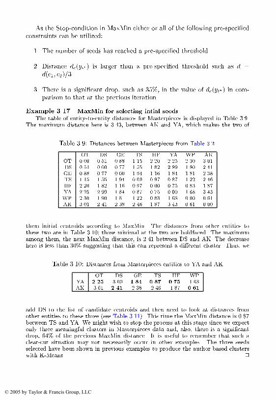
���� INITIALIZATION OF K�MEANS ��
As the Stopcondition in MaxMin either or all of the following prespeciedconstraints can be utilized�
�� The number of seeds has reached a prespecied threshold�
�� Distance dc�yi�� is larger than a prespecied threshold such as d �d�c�� c�����
�� There is a signicant drop� such as �� � in the value of dc�yi�� in comparison to that at the previous iteration�
Example ����� MaxMin for selecting intial seeds
The table of entity�to�entity distances for Masterpieces is displayed in Table ����The maximum distance here is ���� between AK and YA which makes the two of
Table ���� Distances between Masterpieces from Table ����
OT DS GE TS HF YA WP AKOT ���� ���� ���� ���� ���� ���� ���� ����DS ���� ���� ���� ���� ���� �� ��� ���GE ���� ���� ���� �� ���� ��� ���� ����TS ���� ���� �� ���� ��� ���� ���� ���HF ���� ���� ���� ��� ���� ���� ���� ����YA ���� �� ��� ���� ���� ���� ���� ���WP ���� ��� ���� ���� ���� ���� ���� ����AK ���� ��� ���� ��� ���� ��� ���� ����
them initial centroids according to MaxMin� The distances from other entities tothese two are in Table ���� those minimal at the two are boldfaced� The maximumamong them the next MaxMin distance is ���� between DS and AK� The decreasehere is less than �� suggesting that this can represent a di�erent cluster� Thus we
Table ����� Distances from Masterpieces entities to YA and AK
OT DS GE TS HF WPYA ���� ���� ��� ��� ���� ����AK ���� ���� ���� ��� ���� ���
add DS to the list of candidate centroids and then need to look at distances fromother entities to these three �see Table ���� � This time the MaxMin distance is ���between TS and YA� We might wish to stop the process at this stage since we expectonly three meaningful clusters in Masterpieces data and also there is a signi�cantdrop ��� of the previous MaxMin distance� It is useful to remember that such aclear�cut situation may not necessarily occur in other examples� The three seedsselected have been shown in previous examples to produce the author based clusterswith K�Means� �
© 2005 by Taylor & Francis Group, LLC
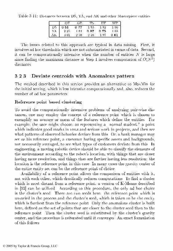
�� K�MEANS CLUSTERING
Table ����� Distances between DS YA and AK and other Masterpiece entities�
OT GE TS HF WPDS ���� ���� ���� ���� ���YA ���� ��� ��� ���� ����AK ���� ���� ��� ���� ���
The issues related to this approach are typical in data mining� First� itinvolves ad hoc thresholds which are not substantiated in terms of data� Second�it can be computationally intensive when the number of entities N is largesince nding the maximum distance at Step � involves computation of O�N��distances�
����� Deviate centroids with Anomalous pattern
The method described in this section provides an alternative to MaxMin forthe initial setting� which is less intensive computationally and� also� reduces thenumber of ad hoc parameters�
Reference point based clustering
To avoid the computationally intensive problems of analyzing pairwise distances� one may employ the concept of a reference point which is chosen toexemplify an average or norm of the features which dene the entities� Forexample� the user might choose� as representing a �normal student�� a pointwhich indicates good marks in tests and serious work in projects� and then seewhat patterns of observed behavior deviate from this� Or� a bank manager mayset as his reference point� a customer having specic assets and backgrounds�not necessarily averaged� to see what types of customers deviate from this� Inengineering� a moving robotic device should be able to classify the elements ofthe environment according to the robot�s location� with things that are closerhaving more resolution� and things that are farther having less resolution� thelocation is the reference point in this case� In many cases the gravity center ofthe entire entity set can be the reference point of choice�Availability of a reference point allows the comparison of entities with it�
not with each other� which drastically reduces computations� To nd a clusterwhich is most distant from a reference point� a version of KMeans describedin ���� can be utilized� According to this procedure� the only ad hoc choiceis the cluster�s seed� There are two seeds here� the reference point which isunvaried in the process and the cluster�s seed� which is taken to be the entitywhich is farthest from the reference point� Only the anomalous cluster is builthere� dened as the set of points that are closer to the cluster seed than to thereference point� Then the cluster seed is substituted by the cluster�s gravitycenter� and the procedure is reiterated until it converges� An exact formulationof this follows�
© 2005 by Taylor & Francis Group, LLC
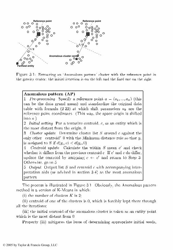
���� INITIALIZATION OF K�MEANS ��
Reference point
Farthest entity
1 / 2
Reference point
1 / 2
Anomalous cluster center
Figure ���� Extracting an Anomalous pattern� cluster with the reference point inthe gravity center� the initial iteration is on the left and the �nal one on the right�
Anomalous pattern �AP��� Pre�processing� Specify a reference point a � �a�� ���� an� �thiscan be the data grand mean� and standardize the original datatable with formula ������ at which shift parameters ak are thereference point coordinates� �This way� the space origin is shiftedinto a���� Initial setting� Put a tentative centroid� c� as an entity which isthe most distant from the origin� ���� Cluster update� Determine cluster list S around c against theonly other �centroid� � with the Minimum distance rule so that yiis assigned to S if d�yi� c� � d�yi� ����� Centroid update� Calculate the within S mean c� and checkwhether it di ers from the previous centroid c� If c� and c do di er�update the centroid by assigning c � c� and return to Step ��Otherwise� go to ���� Output� Output list S and centroid c with accompanying interpretation aids �as advised in section ���� as the most anomalouspattern�
The process is illustrated in Figure ���� Obviously� the Anomalous patternmethod is a version of KMeans in which�
�i� the number of clusters K is ��
�ii� centroid of one of the clusters is �� which is forcibly kept there throughall the iterations�
�iii� the initial centroid of the anomalous cluster is taken as an entity pointwhich is the most distant from ��
Property �iii� mitigates the issue of determining appropriate initial seeds�
© 2005 by Taylor & Francis Group, LLC
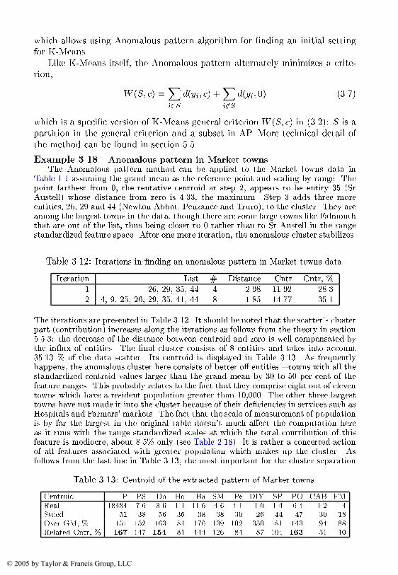
�� K�MEANS CLUSTERING
which allows using Anomalous pattern algorithm for nding an initial settingfor KMeans�Like KMeans itself� the Anomalous pattern alternately minimizes a crite
rion�
W �S� c� �Xi�S
d�yi� c� !Xi��S
d�yi� �� �����
which is a specic version of KMeans general criterion W �S� c� in ������ S is apartition in the general criterion and a subset in AP� More technical detail ofthe method can be found in section ����
Example ����� Anomalous pattern in Market townsThe Anomalous pattern method can be applied to the Market towns data in
Table ��� assuming the grand mean as the reference point and scaling by range� Thepoint farthest from the tentative centroid at step � appears to be entity �� �StAustell whose distance from zero is ���� the maximum� Step � adds three moreentities �� �� and �� �Newton Abbot Penzance and Truro to the cluster� They areamong the largest towns in the data though there are some large towns like Falmouththat are out of the list thus being closer to rather than to St Austell in the rangestandardized feature space� After one more iteration the anomalous cluster stabilizes�
Table ����� Iterations in �nding an anomalous pattern in Market towns data�
Iteration List ! Distance Cntr Cntr �
� �� �� �� �� � ���� ����� ����� � � �� �� �� �� �� �� � ���� ����� ����
The iterations are presented in Table ����� It should be noted that the scatter�s clusterpart �contribution increases along the iterations as follows from the theory in section������ the decrease of the distance between centroid and zero is well compensated bythe in"ux of entities� The �nal cluster consists of � entities and takes into account����� � of the data scatter� Its centroid is displayed in Table ����� As frequentlyhappens the anomalous cluster here consists of better o� entities � towns with all thestandardized centroid values larger than the grand mean by � to � per cent of thefeature ranges� This probably relates to the fact that they comprise eight out of eleventowns which have a resident population greater than �� The other three largesttowns have not made it into the cluster because of their de�ciencies in services such asHospitals and Farmers� markets� The fact that the scale of measurement of populationis by far the largest in the original table doesn�t much a�ect the computation hereas it runs with the range standardized scales at which the total contribution of thisfeature is mediocre about ���� only �see Table ���� � It is rather a concerted actionof all features associated with greater population which makes up the cluster� Asfollows from the last line in Table ���� the most important for the cluster separation
Table ����� Centroid of the extracted pattern of Market towns�
Centroid P PS Do Ho Ba SM Pe DIY SP PO CAB FMReal ��� ��� ��� ��� ���� �� �� ��� �� �� ��� �Stded ��� ��� ��� ��� ��� ��� ��� ��� � �� ��� ���Over GM� � ��� ��� ��� ��� ��� �� ��� ��� ��� �� ��Related Cntr� � �� �� ��� �� � ��� � �� �� �� �� ��
© 2005 by Taylor & Francis Group, LLC
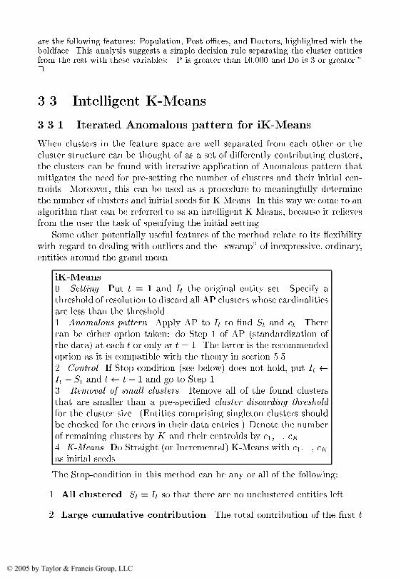
���� INTELLIGENT K�MEANS ��
are the following features� Population Post o�ces and Doctors highlighted with theboldface� This analysis suggests a simple decision rule separating the cluster entitiesfrom the rest with these variables� �P is greater than � and Do is � or greater���
��� Intelligent K�Means
����� Iterated Anomalous pattern for iKMeans
When clusters in the feature space are well separated from each other or thecluster structure can be thought of as a set of di erently contributing clusters�the clusters can be found with iterative application of Anomalous pattern thatmitigates the need for presetting the number of clusters and their initial centroids� Moreover� this can be used as a procedure to meaningfully determinethe number of clusters and initial seeds for KMeans� In this way we come to analgorithm that can be referred to as an intelligent KMeans� because it relievesfrom the user the task of specifying the initial setting�Some other potentially useful features of the method relate to its �exibility
with regard to dealing with outliers and the �swamp� of inexpressive� ordinary�entities around the grand mean�
iK�Means�� Setting� Put t � � and It the original entity set� Specify athreshold of resolution to discard all AP clusters whose cardinalitiesare less than the threshold��� Anomalous pattern� Apply AP to It to nd St and ct� Therecan be either option taken� do Step � of AP �standardization ofthe data� at each t or only at t � �� The latter is the recommendedoption as it is compatible with the theory in section ������ Control� If Stopcondition �see below� does not hold� put It �It � St and t� t! � and go to Step ���� Removal of small clusters� Remove all of the found clustersthat are smaller than a prespecied cluster discarding thresholdfor the cluster size� �Entities comprising singleton clusters shouldbe checked for the errors in their data entries�� Denote the numberof remaining clusters by K and their centroids by c������ cK ��� K�Means� Do Straight �or Incremental� KMeans with c������ cKas initial seeds�
The Stopcondition in this method can be any or all of the following�
�� All clustered� St � It so that there are no unclustered entities left�
�� Large cumulative contribution� The total contribution of the rst t
© 2005 by Taylor & Francis Group, LLC
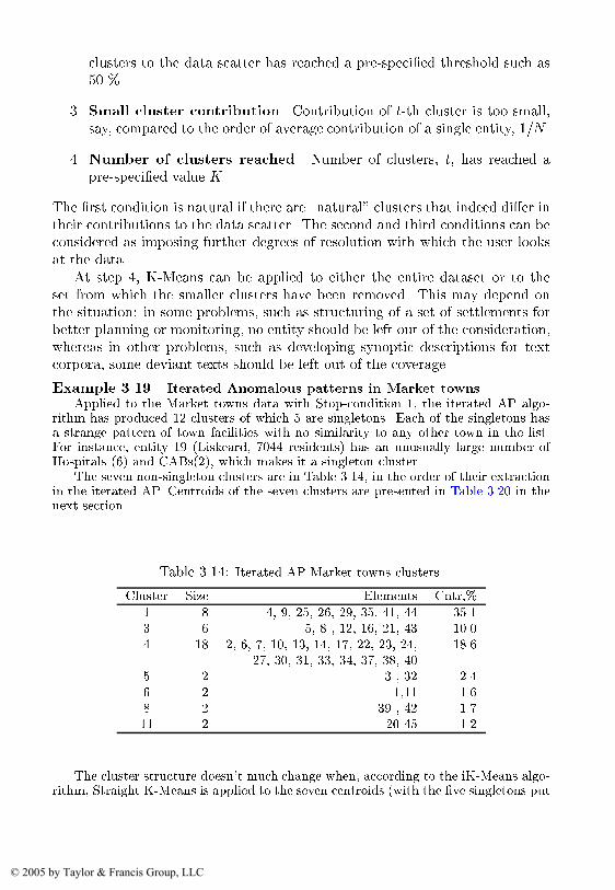
�� K�MEANS CLUSTERING
clusters to the data scatter has reached a prespecied threshold such as�� �
�� Small cluster contribution� Contribution of tth cluster is too small�say� compared to the order of average contribution of a single entity� ��N �
�� Number of clusters reached� Number of clusters� t� has reached aprespecied value K�
The rst condition is natural if there are �natural� clusters that indeed di er intheir contributions to the data scatter� The second and third conditions can beconsidered as imposing further degrees of resolution with which the user looksat the data�At step �� KMeans can be applied to either the entire dataset or to the
set from which the smaller clusters have been removed� This may depend onthe situation� in some problems� such as structuring of a set of settlements forbetter planning or monitoring� no entity should be left out of the consideration�whereas in other problems� such as developing synoptic descriptions for textcorpora� some deviant texts should be left out of the coverage�
Example ����� Iterated Anomalous patterns in Market townsApplied to the Market towns data with Stop�condition � the iterated AP algo�
rithm has produced �� clusters of which � are singletons� Each of the singletons hasa strange pattern of town facilities with no similarity to any other town in the list�For instance entity �� �Liskeard ��� residents has an unusually large number ofHospitals �� and CABs�� which makes it a singleton cluster�
The seven non�singleton clusters are in Table ���� in the order of their extractionin the iterated AP� Centroids of the seven clusters are presented in Table ��� in thenext section�
Table ����� Iterated AP Market towns clusters�
Cluster Size Elements Cntr�
� � � � �� �� �� �� �� �� ����� � � � �� �� �� �� ��� �� � � � � �� �� �� �� �� �� ����
�� � �� �� �� �� �� �� � � �� ���� � ��� ���� � �� �� ����� � � �� ���
The cluster structure doesn�t much change when according to the iK�Means algo�rithm Straight K�Means is applied to the seven centroids �with the �ve singletons put
© 2005 by Taylor & Francis Group, LLC
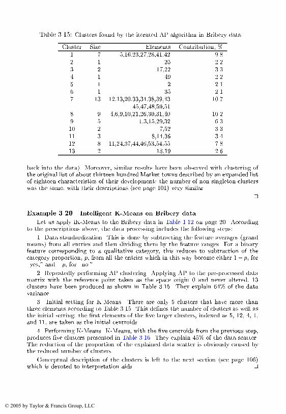
���� INTELLIGENT K�MEANS ��
Table ����� Clusters found by the iterated AP algorithm in Bribery data�
Cluster Size Elements Contribution �
� � ������������� ���� � �� ���� � ���� ���� � �� ���� � � ���� � �� ���� �� ��������������� ���
���������� � ������������ ���� � �������� ���� � ��� ����� � ����� ����� � ���������������� ����� � ���� ���
back into the data � Moreover similar results have been observed with clustering ofthe original list of about thirteen hundred Market towns described by an expanded listof eighteen characteristics of their development� the number of non�singleton clusterswas the same with their descriptions �see page �� very similar�
�
Example ���� Intelligent K Means on Bribery data
Let us apply iK�Means to the Bribery data in Table ���� on page �� Accordingto the prescriptions above the data processing includes the following steps�
�� Data standardization� This is done by subtracting the feature averages �grandmeans from all entries and then dividing them by the feature ranges� For a binaryfeature corresponding to a qualitative category this reduces to subtraction of thecategory proportion p from all the entries which in this way become either �� p for�yes� and �p for �no��
�� Repeatedly performing AP clustering� Applying AP to the pre�processed datamatrix with the reference point taken as the space origin and never altered ��clusters have been produced as shown in Table ����� They explain ��� of the datavariance�
�� Initial setting for K�Means� There are only � clusters that have more thanthree elements according to Table ����� This de�nes the number of clusters as well asthe initial setting� the �rst elements of the �ve larger clusters indexed as � �� � �and �� are taken as the initial centroids�
�� Performing K�Means� K�Means with the �ve centroids from the previous stepproduces �ve clusters presented in Table ����� They explain ��� of the data scatter�The reduction of the proportion of the explained data scatter is obviously caused bythe reduced number of clusters�
Conceptual description of the clusters is left to the next section �see page �� which is devoted to interpretation aids� �
© 2005 by Taylor & Francis Group, LLC
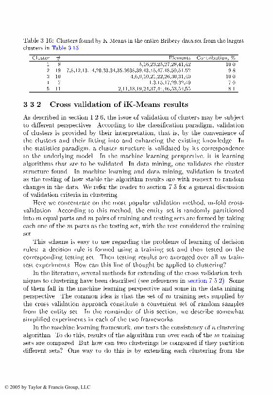
�� K�MEANS CLUSTERING
Table ����� Clusters found by K�Means in the entire Bribery data set from the largestclusters in Table �����
Cluster � Elements Contribution� �� � �������������������� ����� � ���������������������������������������������� ��� �� ����������������������� ���� � ��������������� ���� �� ������������������������� ���
����� Cross validation of iKMeans results
As described in section ������ the issue of validation of clusters may be subjectto di erent perspectives� According to the classication paradigm� validationof clusters is provided by their interpretation� that is� by the convenience ofthe clusters and their tting into and enhancing the existing knowledge� Inthe statistics paradigm� a cluster structure is validated by its correspondenceto the underlying model� In the machine learning perspective� it is learningalgorithms that are to be validated� In data mining� one validates the clusterstructure found� In machine learning and data mining� validation is treatedas the testing of how stable the algorithm results are with respect to randomchanges in the data� We refer the reader to section ��� for a general discussionof validation criteria in clustering�
Here we concentrate on the most popular validation method� mfold crossvalidation� According to this method� the entity set is randomly partitionedinto m equal parts and m pairs of training and testing sets are formed by takingeach one of the m parts as the testing set� with the rest considered the trainingset�
This scheme is easy to use regarding the problems of learning of decisionrules� a decision rule is formed using a training set and then tested on thecorresponding testing set� Then testing results are averaged over all m traintest experiments� How can this line of thought be applied to clustering�
In the literature� several methods for extending of the crossvalidation techniques to clustering have been described �see references in section ������� Someof them fall in the machine learning perspective and some in the data miningperspective� The common idea is that the set of m training sets supplied bythe cross validation approach constitute a convenient set of random samplesfrom the entity set� In the remainder of this section� we describe somewhatsimplied experiments in each of the two frameworks�
In the machine learning framework� one tests the consistency of a clusteringalgorithm� To do this� results of the algorithm run over each of the m trainingsets are compared� But how can two clusterings be compared if they partitiondi erent sets� One way to do this is by extending each clustering from the
© 2005 by Taylor & Francis Group, LLC
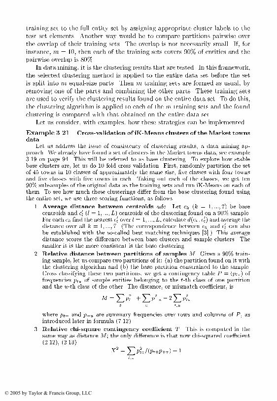
���� INTELLIGENT K�MEANS ��
training set to the full entity set by assigning appropriate cluster labels to thetest set elements� Another way would be to compare partitions pairwise overthe overlap of their training sets� The overlap is not necessarily small� If� forinstance� m � ��� then each of the training sets covers �� of entities and thepairwise overlap is �� �In data mining� it is the clustering results that are tested� In this framework�
the selected clustering method is applied to the entire data set before the setis split into m equalsize parts� Then m training sets are formed as usual� byremoving one of the parts and combining the other parts� These training setsare used to verify the clustering results found on the entire data set� To do this�the clustering algorithm is applied to each of the m training sets and the foundclustering is compared with that obtained on the entire data set�Let us consider� with examples� how these strategies can be implemented�
Example ����� Cross validation of iK Means clusters of the Market townsdata
Let us address the issue of consistency of clustering results a data mining ap�proach� We already have found a set of clusters in the Market towns data see example���� on page ��� This will be referred to as base clustering� To explore how stablebase clusters are let us do ��fold cross�validation� First randomly partition the setof �� towns in � classes of approximately the same size �ve classes with four townsand �ve classes with �ve towns in each� Taking out each of the classes we get ten�� subsamples of the original data as the training sets and run iK�Means on each ofthem� To see how much these clusterings di�er from the base clustering found usingthe entire set we use three scoring functions as follows�
�� Average distance between centroids adc� Let ck �k � �� ���� � be basecentroids and c�l �l � �� ���� L centroids of the clustering found on a �� sample�For each ck �nd the nearest c�l over l � �� ���� L calculate d�ck� c
�l and average the
distance over all k � �� ���� �� �The correspondence between ck and c�l can alsobe established with the so�called best matching techniques #�$� This averagedistance scores the di�erence between base clusters and sample clusters� Thesmaller it is the more consistent is the base clustering�
�� Relative distance between partitions of samples M � Given a �� train�ing sample let us compare two partitions of it� �a the partition found on it withthe clustering algorithm and �b the base partition constrained to the sample�Cross classifying these two partitions we get a contingency table P � �ptu offrequencies ptu of sample entities belonging to the t�th class of one partitionand the u�th class of the other� The distance or mismatch coe�cient is
M �Xt
p�t� �Xu
p��u � �Xt�u
p�tu
where pt� and p�u are summary frequencies over rows and columns of P asintroduced later in formula ����� �
�� Relative chi square contingency coe�cient T � This is computed in thesame way as distance M � the only di�erence is that now chi�squared coe�cient����� �����
X� �Xt�u
p�tu��pt�p�u � �
© 2005 by Taylor & Francis Group, LLC
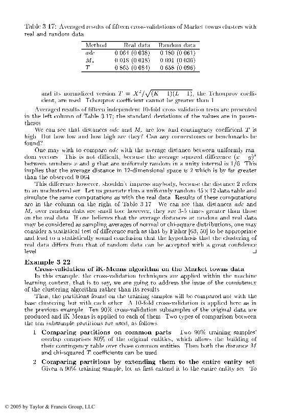
�� K�MEANS CLUSTERING
Table ����� Averaged results of �fteen cross�validations of Market towns clusters withreal and random data�
Method Real data Random data
adc ��� ���� ��� ���� Ms ��� ���� ��� ���� T ���� ���� ���� ����
and its normalized version T � X��p
�K � � �L� � the Tchouprov coe��cient are used� Tchouprov coe�cient cannot be greater than ��
Averaged results of �fteen independent ��fold cross validation tests are presentedin the left column of Table ����� the standard deviations of the values are in paren�theses�
We can see that distances adc and Ms are low and contingency coe�cient T ishigh� But how low and how high are they� Can any cornerstones or benchmarks befound�
One may wish to compare adc with the average distance between uniformly ran�dom vectors� This is not di�cult because the average squared di�erence �x � y �
between numbers x and y that are uniformly random in a unity interval is ���� Thisimplies that the average distance in ���dimensional space is � which is by far greaterthan the observed ����
This di�erence however shouldn�t impress anybody because the distance � refersto an unclustered set� Let us generate thus a uniformly random ����� data table andsimulate the same computations as with the real data� Results of these computationsare in the column on the right of Table ����� We can see that distances adc andMs over random data are small too� however they are ��� times greater than thoseon the real data� If one believes that the average distances at random and real datamay be considered as sampling averages of normal or chi�square distributions one mayconsider a statistical test of di�erence such as that by Fisher #�� �$ to be appropriateand lead to a statistically sound conclusion that the hypothesis that the clustering ofreal data di�ers from that of random data can be accepted with a great con�dencelevel� �
Example �����Cross validation of iK Means algorithm on the Market towns dataIn this example the cross�validation techniques are applied within the machine
learning context that is to say we are going to address the issue of the consistencyof the clustering algorithm rather than its results�
Thus the partitions found on the training samples will be compared not with thebase clustering but with each other� A ��fold cross�validation is applied here as inthe previous example� Ten �� cross�validation subsamples of the original data areproduced and iK�Means is applied to each of them� Two types of comparison betweenthe ten subsample partitions are used as follows�
�� Comparing partitions on common parts� Two �� training samples�overlap comprises �� of the original entities which allows the building oftheir contingency table over those common entities� Then both the distance Mand chi�squared T coe�cients can be used�
�� Comparing partitions by extending them to the entire entity set�Given a �� training sample let us �rst extend it to the entire entity set� To
© 2005 by Taylor & Francis Group, LLC
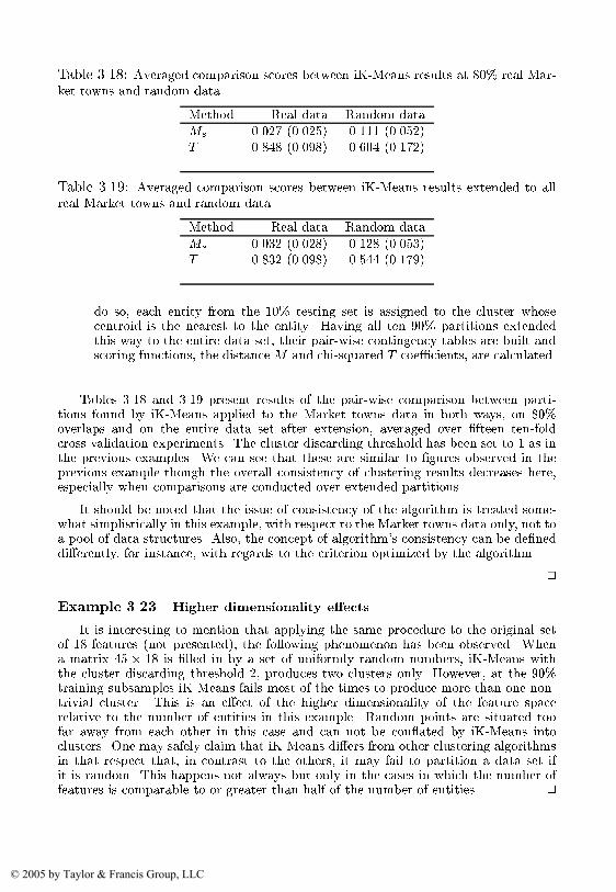
���� INTELLIGENT K�MEANS ��
Table ����� Averaged comparison scores between iK�Means results at �� real Mar�ket towns and random data�
Method Real data Random data
Ms ��� ���� ���� ���� T ���� ���� ��� �����
Table ����� Averaged comparison scores between iK�Means results extended to allreal Market towns and random data�
Method Real data Random data
Ms ��� ���� ���� ���� T ���� ���� ���� �����
do so each entity from the �� testing set is assigned to the cluster whosecentroid is the nearest to the entity� Having all ten �� partitions extendedthis way to the entire data set their pair�wise contingency tables are built andscoring functions the distance M and chi�squared T coe�cients are calculated�
Tables ���� and ���� present results of the pair�wise comparison between parti�tions found by iK�Means applied to the Market towns data in both ways on ��overlaps and on the entire data set after extension averaged over �fteen ten�foldcross�validation experiments� The cluster discarding threshold has been set to � as inthe previous examples� We can see that these are similar to �gures observed in theprevious example though the overall consistency of clustering results decreases hereespecially when comparisons are conducted over extended partitions�
It should be noted that the issue of consistency of the algorithm is treated some�what simplistically in this example with respect to the Market towns data only not toa pool of data structures� Also the concept of algorithm�s consistency can be de�neddi�erently for instance with regards to the criterion optimized by the algorithm�
�
Example ����� Higher dimensionality e�ects
It is interesting to mention that applying the same procedure to the original setof �� features �not presented the following phenomenon has been observed� Whena matrix �� � �� is �lled in by a set of uniformly random numbers iK�Means withthe cluster discarding threshold � produces two clusters only� However at the ��training subsamples iK�Means fails most of the times to produce more than one non�trivial cluster� This is an e�ect of the higher dimensionality of the feature spacerelative to the number of entities in this example� Random points are situated toofar away from each other in this case and can not be con"ated by iK�Means intoclusters� One may safely claim that iK�Means di�ers from other clustering algorithmsin that respect that in contrast to the others it may fail to partition a data set ifit is random� This happens not always but only in the cases in which the number offeatures is comparable to or greater than half of the number of entities� �
© 2005 by Taylor & Francis Group, LLC
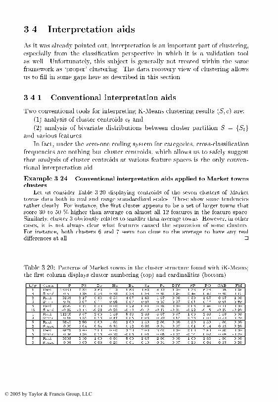
��� K�MEANS CLUSTERING
��� Interpretation aids
As it was already pointed out� interpretation is an important part of clustering�especially from the classication perspective in which it is a validation toolas well� Unfortunately� this subject is generally not treated within the sameframework as �proper� clustering� The data recovery view of clustering allowsus to ll in some gaps here as described in this section�
����� Conventional interpretation aids
Two conventional tools for interpreting KMeans clustering results �S� c� are�
��� analysis of cluster centroids ct and
��� analysis of bivariate distributions between cluster partition S � fStgand various features�
In fact� under the zeroone coding system for categories� crossclassicationfrequencies are nothing but cluster centroids� which allows us to safely suggestthat analysis of cluster centroids at various feature spaces is the only conventional interpretation aid�
Example ����� Conventional interpretation aids applied to Market townsclusters�
Let us consider Table ��� displaying centroids of the seven clusters of Markettowns data both in real and range standardized scales� These show some tendenciesrather clearly� For instance the �rst cluster appears to be a set of larger towns thatscore � to � � higher than average on almost all �� features in the feature space�Similarly cluster � obviously relates to smaller than average towns� However in othercases it is not always clear what features caused the separation of some clusters�For instance both clusters � and � seem too close to the average to have any realdi�erences at all� �
Table ����� Patterns of Market towns in the cluster structure found with iK�Means�the �rst column displays cluster numbering �top and cardinalities �bottom �
k�� Centr P PS Do Ho Ba Su Pe DIY SP PO CAB FM
� Real ����� �� � ��� ��� �� ��� ���� ��� �� ���� ���� Stand ���� ��� ��� �� ��� ��� ��� ��� ���� ���� ��� ����
� Real ��� ���� ��� ���� ��� ��� ��� ���� ���� ��� ��� ���� Stand ���� ���� ���� ���� ���� ���� ���� ���� ���� ���� ���� ����
Real ���� ���� ���� ���� ���� ��� ���� ���� ��� ���� ���� ������ Stand ���� ���� ���� ���� ��� ���� ���� ���� ���� ���� ���� ����
� Real ����� �� ���� �� �� �� �� ��� ���� �� �� ���� Stand ���� ���� ��� ���� ���� ��� ��� ���� ��� ���� ��� ����
� Real ��� ���� ���� ���� ���� ���� ���� ���� ���� ���� ���� ����� Stand ���� ���� ��� ��� ���� ��� ���� ���� ���� ���� ���� ����
Real ��� ��� ���� ���� ��� ���� ���� ���� ���� ���� ���� ����� Stand ��� ��� ��� ���� ��� ���� ���� ���� ���� ���� ���� ����
� Real ��� ���� ���� ���� ���� ��� ���� ���� ���� �� ���� ���� Stand ���� ���� ���� ���� ���� ���� ���� ���� ��� ���� ���� ����
© 2005 by Taylor & Francis Group, LLC
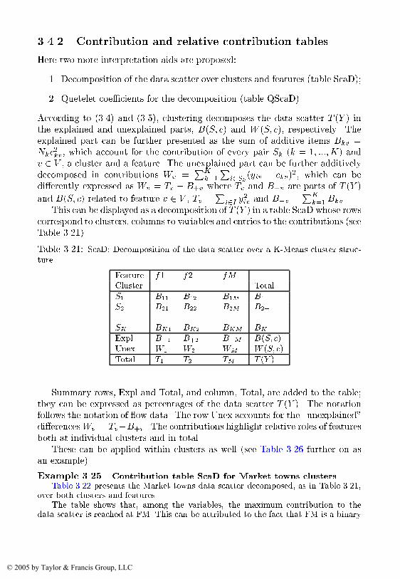
���� INTERPRETATION AIDS ���
����� Contribution and relative contribution tables
Here two more interpretation aids are proposed�
�� Decomposition of the data scatter over clusters and features �table ScaD��
�� Quetelet coe�cients for the decomposition �table QScaD��
According to ����� and ������ clustering decomposes the data scatter T �Y � inthe explained and unexplained parts� B�S� c� and W �S� c�� respectively� Theexplained part can be further presented as the sum of additive items Bkv �Nkc
�kv � which account for the contribution of every pair Sk �k � �� ����K� and
v � V � a cluster and a feature� The unexplained part can be further additivelydecomposed in contributions Wv �
PKk��
Pi�Sk
�yiv � ckv��� which can be
di erently expressed as Wv � Tv � B�v where Tv and B�v are parts of T �Y �
and B�S� c� related to feature v � V � Tv �P
i�I y�iv and B�v �
PKk��Bkv �
This can be displayed as a decomposition of T �Y � in a table ScaD whose rowscorrespond to clusters� columns to variables and entries to the contributions �seeTable ������
Table ����� ScaD� Decomposition of the data scatter over a K�Means cluster struc�ture�
Feature f� f� fMCluster Total
S� B�� B�� B�M B��
S� B�� B�� B�M B��
SK BK� BK� BKM BK�
Expl B�� B�� B�M B�S� c Unex W� W� WM W �S� c
Total T� T� TM T �Y
Summary rows� Expl and Total� and column� Total� are added to the table�they can be expressed as percentages of the data scatter T �Y �� The notationfollows the notation of �ow data� The row Unex accounts for the �unexplained�di erencesWv � Tv�B�v� The contributions highlight relative roles of featuresboth at individual clusters and in total�These can be applied within clusters as well �see Table ���� further on as
an example��
Example ����� Contribution table ScaD for Market towns clustersTable ���� presents the Market towns data scatter decomposed as in Table ����
over both clusters and features�The table shows that among the variables the maximum contribution to the
data scatter is reached at FM� This can be attributed to the fact that FM is a binary
© 2005 by Taylor & Francis Group, LLC
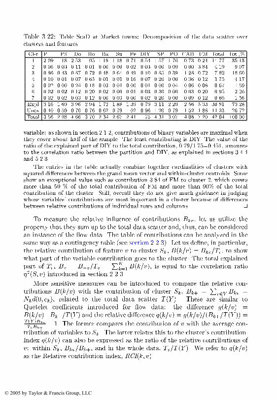
��� K�MEANS CLUSTERING
Table ����� Table ScaD at Market towns� Decomposition of the data scatter overclusters and features�
Cl�r P PS Do Ho Ba Su Pe DIY SP PO CAB FM Total Tot���� ��� ���� ���� ���� ��� ���� ���� ��� ���� ���� ���� ��� ���� ������ ���� ���� ���� ���� ���� ���� ���� ���� ���� ��� ���� ��� �� ��� ���� ��� ���� ���� ��� ��� �� ���� ���� ��� ���� ���� ���� ����� ���� ���� ���� ���� ���� ���� ���� ���� ���� ���� ���� ���� ���� ���� ���� ���� ��� ���� ���� ���� ���� ���� ���� ��� ���� ���� ���� ���� ���� ���� ���� ���� ���� ���� ���� ���� ���� ���� ���� ���� ��� ����� ���� ���� ���� ���� ���� ���� ���� ���� ���� ���� ��� ���� ���� ����
Expl ���� ��� ��� �� ���� ���� ��� ��� ���� ��� ���� ���� ����� �����Unex ��� ��� ���� ���� ���� ��� ���� ��� ���� ��� ���� ���� ����� �����Total ���� ���� ��� ���� ��� ���� ��� ���� ��� ���� ��� ���� ��� ������
variable� as shown in section ����� contributions of binary variables are maximal whenthey cover about half of the sample� The least contributing is DIY� The value of theratio of the explained part of DIY to the total contribution ������������� amountsto the correlation ratio between the partition and DIY as explained in sections �����and ������
The entries in the table actually combine together cardinalities of clusters withsquared di�erences between the grand mean vector and within�cluster centroids� Someshow an exceptional value such as contribution ���� of FM to cluster � which coversmore than � � of the total contribution of FM and more than �� of the totalcontribution of the cluster� Still overall they do not give much guidance in judgingwhose variables� contributions are most important in a cluster because of di�erencesbetween relative contributions of individual rows and columns� �
To measure the relative in�uence of contributions Bkv � let us utilize theproperty that they sum up to the total data scatter and� thus� can be consideredan instance of the �ow data� The table of contributions can be analyzed in thesame way as a contingency table �see section ������� Let us dene� in particular�the relative contribution of feature v to cluster Sk� B�k�v� � Bkv�Tv� to showwhat part of the variable contribution goes to the cluster� The total explainedpart of Tv� Bv � B�v�Tv �
PKk�� B�k�v�� is equal to the correlation ratio
��S� v� introduced in section ������
More sensitive measures can be introduced to compare the relative contributions B�k�v� with the contribution of cluster Sk� Bk� �
Pv�V Bkv �
Nkd��� ck�� related to the total data scatter T �Y �� These are similar toQuetelet coe�cients introduced for �ow data� the di erence g�k�v� �B�k�v��Bk��T �Y � and the relative di erence q�k�v� � g�k�v���Bk��T �Y �� �T �Y �Bkv
TvBk�� �� The former compares the contribution of v with the average con
tribution of variables to Sk� The latter relates this to the cluster�s contribution�Index q�k�v� can also be expressed as the ratio of the relative contributions ofv� within Sk� Bkv�Bk�� and in the whole data� Tv�T �Y �� We refer to q�k�v�as the Relative contribution index� RCI�k� v��
© 2005 by Taylor & Francis Group, LLC
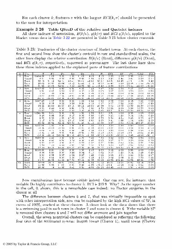
���� INTERPRETATION AIDS ���
For each cluster k� features v with the largest RCI�k� v� should be presentedto the user for interpretation�
Example ����� Table QScaD of the relative and Quetelet indexes
All three indexes of association B�k�v g�k�v and RCI q�k�v applied to theMarket towns data in Table ���� are presented in Table ���� below cluster centroids�
Table ����� Tendencies of the cluster structure of Market towns� At each cluster the�rst and second lines show the cluster�s centroid in raw and standardized scales� theother lines display the relative contribution B�k�v �Rcnt di�erence g�k�v �Dcnt and RCI q�k� v respectively expressed as percentages� The last three lines showthese three indexes applied to the explained parts of feature contributions�
k C d P PS Do Ho Ba Su Pe DIY SP PO CAB FM
� Real �������� �� � ��� ��� �� ��� ���� ��� �� ���� ���Stand ���� ��� ��� �� ��� ��� ��� ��� ���� ���� ��� ����Rcnt ����� ����� ����� ����� ���� ���� ���� ��� �� ���� ����� ���Dcnt ��� ��� ����� ��� ����� ���� ��� ��� ��� ����� ����� ���RCI ��� ��� ����� ����� ����� ���� ���� ���� �� ��� ����� ����
� Real ����� ���� ��� ���� ��� ��� ��� ���� ���� ��� ��� ����Stand ���� ���� ���� ���� ���� ���� ���� ���� ���� ���� ���� ����Rcnt ���� �� ��� ���� ���� ���� ��� ���� ���� ���� ���� ��Dcnt ��� ��� ���� ���� ���� ��� ���� ���� ���� ���� ���� ��RCI ����� ��� ���� ���� ����� ����� ����� ����� ���� ����� ����� �����
Real ������� ���� ���� ���� ���� ��� ���� ���� ��� ���� ���� ����Stand ���� ���� ���� ���� ��� ���� ���� ���� ���� ���� ���� ����Rcnt ����� ����� ���� ���� ���� ���� ���� �� ���� ����� ��� �����Dcnt ���� ���� ���� ��� ���� ��� ���� ���� ���� ���� ����� ���RCI ���� ��� ���� �� ���� ��� ��� ���� ��� ���� ���� ���
� Real ������ �� ���� �� �� �� �� ��� ���� �� �� ����Stand ���� ���� ��� ���� ���� ��� ��� ���� ��� ���� ��� ����Rcnt ���� ��� ��� ��� ��� ��� ��� �� ���� ��� ��� ���Dcnt ���� ��� ��� ���� ��� ��� ��� ���� ��� ���� ��� ����RCI ��� ����� ��� ���� ����� ����� ��� ���� ��� ���� ������ ����
� Real ������ ���� ���� ���� ���� ���� ���� ���� ���� ���� ���� ����Stand ���� ���� ��� ��� ���� ��� ���� ���� ���� ���� ���� ����Rcnt ���� ���� ���� ��� ��� ���� ���� �� ���� ���� ���� ����Dcnt ���� ��� ��� ��� �� ��� ���� ���� ���� ��� ���� ����RCI ����� ����� ������ ����� ���� ���� ����� �� ����� ����� ���� ����
Real ����� ��� ���� ���� ��� ���� ���� ���� ���� ���� ���� ����Stand ��� ��� ��� ���� ��� ���� ���� ���� ���� ���� ���� ����Rcnt ���� ���� ��� ���� ��� ���� ���� ��� �� ���� ���� ����Dcnt ���� ��� ��� ��� ��� ���� ���� ��� ��� ���� ���� ����RCI ����� ���� ����� ����� ��� ����� ���� ��� ���� ���� ���� �����
� Real ������ ���� ���� ���� ���� ��� ���� ���� ���� �� ���� ����Stand ���� ���� ���� ���� ���� ���� ���� ���� ��� ���� ���� ����Rcnt ���� ���� ���� ��� ���� ��� ���� ���� ���� ��� �� ���Dcnt ���� ��� ���� ��� ��� �� ��� ��� ���� ��� ��� ����RCI ���� ���� ��� ������ ����� ����� ���� ���� ����� ����� ���� ���
Ex� Rcnt ���� ����� ����� ����� ���� ���� ����� ����� ����� ����� ���� ���Dcnt ��� ��� ���� ��� ��� ���� ���� ����� ���� ���� ����� ���RCI ���� ���� ���� ���� ��� ��� ���� ���� ��� ��� ���� ���
Now contributions have become visible indeed� One can see for instance thatvariable Do highly contributes to cluster �� RCI is ������ Why� As the upper numberin the cell shows this is a remarkable case indeed� no Doctor surgeries in thecluster at all�
The di�erence between clusters � and � that was virtually impossible to spotwith other interpretation aids now can be explained by the high RCI values of SP inexcess of �� reached at these clusters� A closer look at the data shows that thereis a swimming pool in each town in cluster � and none in cluster �� If the variable SPis removed then clusters � and � will not di�er anymore and join together�
Overall the seven nontrivial clusters can be considered as re"ecting the followingfour tiers of the settlement system� largest towns �Cluster � small towns �Cluster
© 2005 by Taylor & Francis Group, LLC
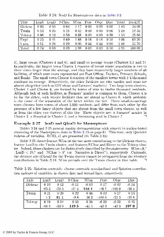
��� K�MEANS CLUSTERING
Table ����� ScaD for Masterpieces data in Table ����
Title LenS LenD NChar SCon Pers Obje Dire Total Total�
Dickens �� �� �� ���� � �� �� ���� ����Twain ��� ��� ��� ��� �� � �� ��� �����Tolstoy �� ��� �� ��� �� �� ��� ���� �����
Expl ��� ��� ��� ���� ��� ��� �� ��� ����Unex ��� ��� �� � ��� ��� � ���� ����
Total ��� ��� ��� ���� ��� ��� �� ���� ��
� large towns �Clusters � and � and small�to�average towns �Clusters �� and � �In particular the largest town Cluster � consists of towns whose population is two tothree times larger than the average and they have respectively larger numbers of allfacilities of which even more represented are Post O�ces Doctors Primary Schoolsand Banks� The small town Cluster � consists of the smallest towns with ��� thousandresidents on average� Respectively the other facilities are also smaller and some areabsent altogether �such as DIY shops and Farmers� markets � Two large town clustersCluster � and Cluster � are formed by towns of nine to twelve thousand residents�Although lack of such facilities as Farmers� market is common to them Cluster � isby far the richer with service facilities that are absent in Cluster � which probablyis the cause of the separation of the latter within the tier� Three small�to�averagetown clusters have towns of about � residents and di�er from each other by thepresence of a few fancy objects that are absent from the small town cluster as wellas from the other two clusters of this tier� These objects are� a Farmers� market inCluster � a Hospital in Cluster � and a Swimming pool in Cluster �� �
Example ����� ScaD and QScaD for Masterpieces
Tables ���� and ���� present similar decompositions with respect to author�basedclustering of the Masterpieces data in Table ���� on page ��� This time only Queteletindexes of variables RCI�k� v are presented �in Table ���� �
Table ���� shows feature SCon as the one most contributing to the Dickens clusterfeature LenD to the Twain cluster and features NChar and Direct to the Tolstoy clus�ter� Indeed these clusters can be distinctively described by the statements �SCon���LenD � ��� and �NChar � �� �or �Narrative is Direct� respectively� Curiouslythe decisive role of LenD for the Twain cluster cannot be recognized from the absolutecontributions in Table ����� SCon prevails over the Twain cluster in that table� �
Table ����� Relative centroids� cluster centroids standardized and Relative contribu�tion indexes of variables in cluster �rst and second lines respectively�
Title LenS LenD NChar SCon Pers Obje Dire
Dickens �� ��� ���� ���� ��� ��� ��������� ���� ����� ���� ���� ��� ����
Twain ���� ���� ���� ��� ��� ��� ������� ���� ���� ��� ��� ����� �����
Tolstoy ��� ��� �� ��� ���� ���� �������� ���� ���� ����� ����� ����� �����
© 2005 by Taylor & Francis Group, LLC
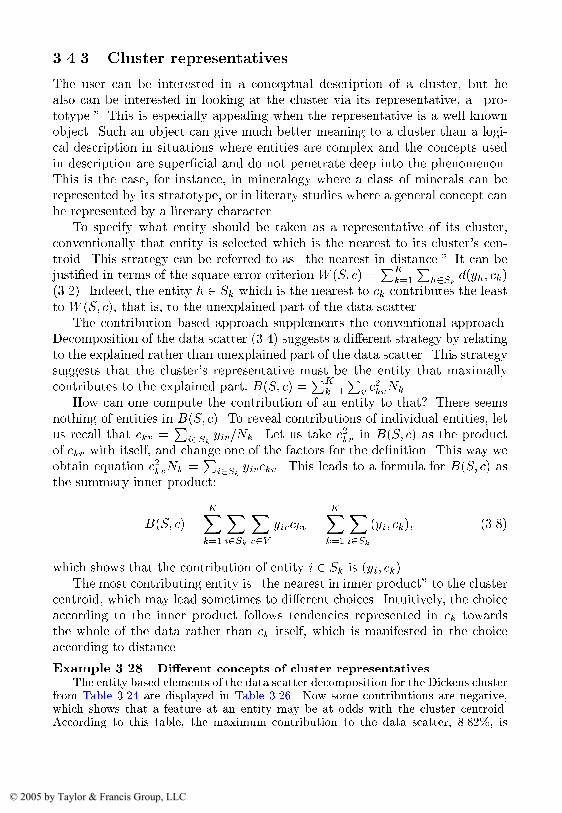
���� INTERPRETATION AIDS ���
����� Cluster representatives
The user can be interested in a conceptual description of a cluster� but healso can be interested in looking at the cluster via its representative� a �prototype�� This is especially appealing when the representative is a well knownobject� Such an object can give much better meaning to a cluster than a logical description in situations where entities are complex and the concepts usedin description are supercial and do not penetrate deep into the phenomenon�This is the case� for instance� in mineralogy where a class of minerals can berepresented by its stratotype� or in literary studies where a general concept canbe represented by a literary character�To specify what entity should be taken as a representative of its cluster�
conventionally that entity is selected which is the nearest to its cluster�s centroid� This strategy can be referred to as �the nearest in distance�� It can bejustied in terms of the square error criterion W �S� c� �
PKk��
Ph�Sk
d�yh� ck������� Indeed� the entity h � Sk which is the nearest to ck contributes the leastto W �S� c�� that is� to the unexplained part of the data scatter�The contribution based approach supplements the conventional approach�
Decomposition of the data scatter ����� suggests a di erent strategy by relatingto the explained rather than unexplained part of the data scatter� This strategysuggests that the cluster�s representative must be the entity that maximallycontributes to the explained part� B�S� c� �
PKk��
Pv c
�kvNk�
How can one compute the contribution of an entity to that� There seemsnothing of entities in B�S� c�� To reveal contributions of individual entities� letus recall that ckv �
Pi�Sk
yiv�Nk� Let us take c�kv in B�S� c� as the product
of ckv with itself� and change one of the factors for the denition� This way weobtain equation c�kvNk �
Pi�Sk
yivckv � This leads to a formula for B�S� c� asthe summary inner product�
B�S� c� �
KXk��
Xi�Sk
Xv�V
yivckv �
KXk��
Xi�Sk
�yi� ck�� �����
which shows that the contribution of entity i � Sk is �yi� ck��The most contributing entity is �the nearest in inner product� to the cluster
centroid� which may lead sometimes to di erent choices� Intuitively� the choiceaccording to the inner product follows tendencies represented in ck towardsthe whole of the data rather than ck itself� which is manifested in the choiceaccording to distance�
Example ����� Di�erent concepts of cluster representativesThe entity based elements of the data scatter decomposition for the Dickens cluster
from Table ���� are displayed in Table ����� Now some contributions are negativewhich shows that a feature at an entity may be at odds with the cluster centroid�According to this table the maximum contribution to the data scatter ����� is
© 2005 by Taylor & Francis Group, LLC
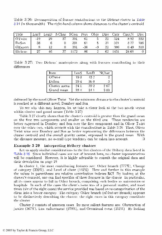
��� K�MEANS CLUSTERING
Table ����� Decomposition of feature contributions to the Dickens cluster in Table���� �in thousandth � The right�hand column shows distances to the cluster�s centroid�
Title LenS LenD NChar SCon Pers Obje Dire Cntr Cntr� Dist
OTwist ��� �� �� ��� �� � �� ��� ���� ���DoSon �� � ��� �� � �� ��� ���� ���GExpect � �� ��� ��� �� �� ��� ���� ��
Dickens �� �� �� ���� �� � �� ���� ����
Table ����� Two Dickens� masterpieces along with features contributing to theirdi�erences�
Item LenS LenD NChar
OTwist ��� ���� �DoSon ���� ��� �
Cluster mean ���� ���� ����Grand mean ���� ���� ��
delivered by the novel Oliver Twist� Yet the minimum distance to the cluster�s centroidis reached at a di�erent novel Dombey and Son�
To see why this may happen let us take a closer look at the two novels versuswithin cluster and grand means �Table ���� �
Table ���� clearly shows that the cluster�s centroid is greater than the grand meanon the �rst two components and smaller on the third one� These tendencies arebetter expressed in Dombey and Son over the �rst component and in Oliver Twistover the other two which accords with the contributions in Table ����� Thus OliverTwist wins over Dombey and Son as better representing the di�erences between thecluster centroid and the overall gravity center expressed in the grand mean� Withthe distance measure no overall type tendency can be taken into account� �
Example ����� Interpreting Bribery clusters
Let us apply similar considerations to the �ve clusters of the Bribery data listed inTable ����� Since individual cases are not of interest here no cluster representativeswill be considered� However it is highly advisable to consult the original data andtheir description on page ���
In cluster � the most contributing features are� Other branch ����� Changeof category ����� and Level of client ����� � Here and further in this examplethe values in parentheses are relative contribution indexes RCI� By looking at thecluster�s centroid one can �nd speci�cs of these features in the cluster� In particularall its cases appear to fall in Other branch comprising such bodies as universities orhospitals� In each of the cases the client�s issue was of a personal matter and mosttimes �six of the eight cases the service provided was based on re�categorization of theclient into a better category� The category Other branch �of feature Branch appearsto be distinctively describing the cluster� the eight cases in this category constitutethe cluster�
Cluster � consists of nineteen cases� Its most salient features are� Obstruction ofjustice ����� Law enforcement ����� and Occasional event ����� � By looking
© 2005 by Taylor & Francis Group, LLC
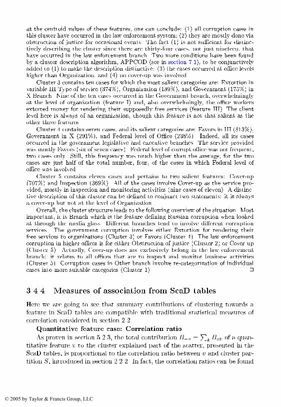
���� INTERPRETATION AIDS ���
at the centroid values of these features one can conclude� �� all corruption cases inthis cluster have occurred in the law enforcement system� �� they are mostly done viaobstruction of justice for occasional events� The fact �� is not su�cient for distinc�tively describing the cluster since there are thirty�four cases not just nineteen thathave occurred in the law enforcement branch� Two more conditions have been foundby a cluster description algorithm APPCOD �see in section ��� to be conjunctivelyadded to �� to make the description distinctive� �� the cases occurred at o�ce levelshigher than Organization and �� no cover�up was involved�
Cluster � contains ten cases for which the most salient categories are� Extortion invariable III Type of service ����� Organization ����� and Government ����� inX Branch� Nine of the ten cases occurred in the Government branch overwhelminglyat the level of organization �feature I and also overwhelmingly the o�ce workersextorted money for rendering their supposedly free services �feature III � The clientlevel here is always of an organization though this feature is not that salient as theother three features�
Cluster � contains seven cases and its salient categories are� Favors in III ����� Government in X ����� and Federal level of O�ce ����� � Indeed all its casesoccurred in the government legislative and executive branches� The service providedwas mostly Favors �six of seven cases � Federal level of corrupt o�ce was not frequenttwo cases only� Still this frequency was much higher than the average for the twocases are just half of the total number four of the cases in which Federal level ofo�ce was involved�
Cluster � contains eleven cases and pertains to two salient features� Cover�up���� and Inspection ����� � All of the cases involve Cover�up as the service pro�vided mostly in inspection and monitoring activities �nine cases of eleven � A distinc�tive description of this cluster can be de�ned to conjunct two statements� it is alwaysa cover�up but not at the level of Organization�
Overall the cluster structure leads to the following overview of the situation� Mostimportant it is Branch which is the feature de�ning Russian corruption when lookedat through the media glass� Di�erent branches tend to involve di�erent corruptionservices� The government corruption involves either Extortion for rendering theirfree services to organizations �Cluster � or Favors �Cluster � � The law enforcementcorruption in higher o�ces is for either Obstruction of justice �Cluster � or Cover�up�Cluster � � Actually Cover�up does not exclusively belong in the law enforcementbranch� it relates to all o�ces that are to inspect and monitor business activities�Cluster � � Corruption cases in Other branch involve re�categorization of individualcases into more suitable categories �Cluster � � �
����� Measures of association from ScaD tables
Here we are going to see that summary contributions of clustering towards afeature in ScaD tables are compatible with traditional statistical measures ofcorrelation considered in section ����
Quantitative feature case� Correlation ratio
As proven in section ������ the total contribution B�v �P
k Bvk of a quantitative feature v to the clusterexplained part of the scatter� presented in theScaD tables� is proportional to the correlation ratio between v and cluster partition S� introduced in section ������ In fact� the correlation ratios can be found
© 2005 by Taylor & Francis Group, LLC
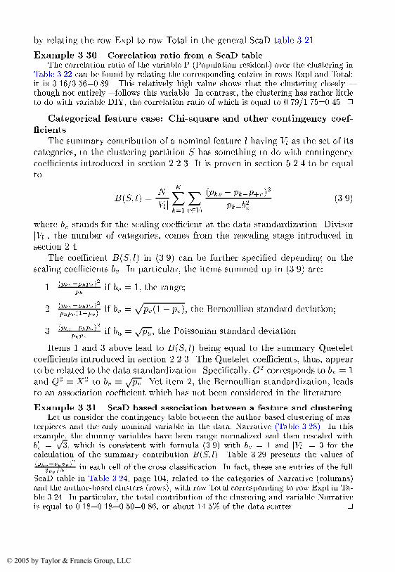
��� K�MEANS CLUSTERING
by relating the row Expl to row Total in the general ScaD table �����
Example ���� Correlation ratio from a ScaD tableThe correlation ratio of the variable P �Population resident over the clustering in
Table ���� can be found by relating the corresponding entries in rows Expl and Total�it is �������������� This relatively high value shows that the clustering closely �though not entirely � follows this variable� In contrast the clustering has rather littleto do with variable DIY the correlation ratio of which is equal to ������������� �
Categorical feature case� Chi�square and other contingency coef��cientsThe summary contribution of a nominal feature l having Vl as the set of its
categories� to the clustering partition S has something to do with contingencycoe�cients introduced in section ������ It is proven in section ����� to be equalto
B�S� l� �N
jVljKXk��
Xv�Vl
�pkv � pk�p�v��
pk�b�v�����
where bv stands for the scaling coe�cient at the data standardization� DivisorjVlj� the number of categories� comes from the rescaling stage introduced insection ����The coe�cient B�S� l� in ����� can be further specied depending on the
scaling coe�cients bv� In particular� the items summed up in ����� are�
�� �pkv�pkpv��
pkif bv � �� the range�
�� �pkv�pkpv��
pkpv���pv�if bv �
ppv��� pv�� the Bernoullian standard deviation�
�� �pkv�pkpv��
pkpvif bu �
ppu� the Poissonian standard deviation�
Items � and � above lead to B�S� l� being equal to the summary Queteletcoe�cients introduced in section ������ The Quetelet coe�cients� thus� appearto be related to the data standardization� Specically� G� corresponds to bv � �and Q� � X� to bv �
ppv� Yet item �� the Bernoullian standardization� leads
to an association coe�cient which has not been considered in the literature�
Example ����� ScaD based association between a feature and clusteringLet us consider the contingency table between the author�based clustering of mas�
terpieces and the only nominal variable in the data Narrative �Table ���� � In thisexample the dummy variables have been range normalized and then rescaled withb�v �
p� which is consistent with formula ���� with bv � � and jVlj � � for the
calculation of the summary contribution B�S� l � Table ���� presents the values of�pkv�pkpv�
�
�pk�Nin each cell of the cross classi�cation� In fact these are entries of the full
ScaD table in Table ���� page �� related to the categories of Narrative �columns and the author�based clusters �rows with row Total corresponding to row Expl in Ta�ble ����� In particular the total contribution of the clustering and variable Narrativeis equal to �������������� or about ����� of the data scatter� �
© 2005 by Taylor & Francis Group, LLC
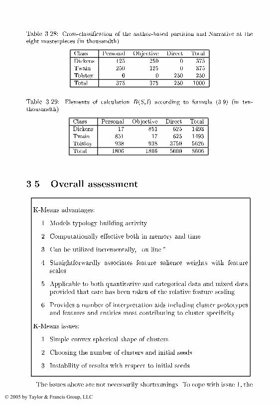
���� OVERALL ASSESSMENT ���
Table ����� Cross�classi�cation of the author�based partition and Narrative at theeight masterpieces �in thousandth �
Class Personal Objective Direct Total
Dickens ��� �� ���Twain �� ��� ���Tolstoy �� ��
Total ��� ��� �� �
Table ����� Elements of calculation B�S� l according to formula ���� �in ten�thousandth �
Class Personal Objective Direct Total
Dickens �� ��� ��� ����Twain ��� �� ��� ����Tolstoy ��� ��� ��� ����
Total ��� ��� � ���
��� Overall assessment
KMeans advantages�
�� Models typology building activity�
�� Computationally e ective both in memory and time�
�� Can be utilized incrementally� �online��
�� Straightforwardly associates feature salience weights with featurescales�
�� Applicable to both quantitative and categorical data and mixed dataprovided that care has been taken of the relative feature scaling�
�� Provides a number of interpretation aids including cluster prototypesand features and entities most contributing to cluster specicity�
KMeans issues�
�� Simple convex spherical shape of clusters�
�� Choosing the number of clusters and initial seeds�
�� Instability of results with respect to initial seeds�
The issues above are not necessarily shortcomings� To cope with issue �� the
© 2005 by Taylor & Francis Group, LLC
��� K�MEANS CLUSTERING
feature set should be chosen carefully according to the goals of the data analysis�To cope with issue �� the initial seeds should be selected based on conceptualunderstanding of the substantive domain or preliminary data analysis with theAP clustering approach� There can be some advantages in the issues as well�Issue � keeps solutions close to prespecied centroid settings� which is goodwhen centroids have been conceptually substantiated� Issue � of simplicity ofcluster shapes provides for a possibility of deriving simple conjunctive descriptions of the clusters� which can be used as supplementary interpretation aids�see section �����A clustering algorithm should present the user with a comfortable set of op
tions to do clustering� In our view� the intelligent version of KMeans describedabove and its versions� implementing the possibility of removal of entities thathave been found either ��� �deviant� �contents of small Anomalous patternclusters�� or ��� �intermediate� �entities that are far away from their centroids�or have small attraction index values�� or ��� �trivial� �entities that are closeto the grand mean�� give the user an opportunity to select a preferred optionwithout imposing on him technical issues�
© 2005 by Taylor & Francis Group, LLC
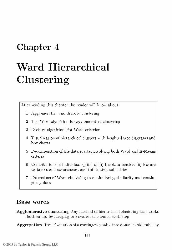
Chapter �
Ward Hierarchical
Clustering
After reading this chapter the reader will know about�
�� Agglomerative and divisive clustering�
�� The Ward algorithm for agglomerative clustering�
�� Divisive algorithms for Ward criterion�
�� Visualization of hierarchical clusters with heighted tree diagrams andbox charts�
�� Decomposition of the data scatter involving both Ward and KMeanscriteria�
�� Contributions of individual splits to� �i� the data scatter� �ii� featurevariances and covariances� and �iii� individual entries�
�� Extensions of Ward clustering to dissimilarity� similarity and contingency data�
Base words
Agglomerative clustering Any method of hierarchical clustering that worksbottom up� by merging two nearest clusters at each step�
Aggregation Transformation of a contingency table into a smaller size table by
���
© 2005 by Taylor & Francis Group, LLC
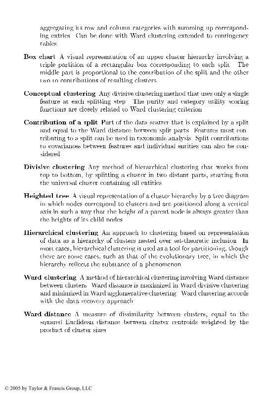
��� WARD HIERARCHICAL CLUSTERING
aggregating its row and column categories with summing up corresponding entries� Can be done with Ward clustering extended to contingencytables�
Box chart A visual representation of an upper cluster hierarchy involving atriple partition of a rectangular box corresponding to each split� Themiddle part is proportional to the contribution of the split and the othertwo to contributions of resulting clusters�
Conceptual clustering Any divisive clustering method that uses only a singlefeature at each splitting step� The purity and category utility scoringfunctions are closely related to Ward clustering criterion�
Contribution of a split Part of the data scatter that is explained by a splitand equal to the Ward distance between split parts� Features most contributing to a split can be used in taxonomic analysis� Split contributionsto covariances between features and individual entities can also be considered�
Divisive clustering Any method of hierarchical clustering that works fromtop to bottom� by splitting a cluster in two distant parts� starting fromthe universal cluster containing all entities�
Heighted tree A visual representation of a cluster hierarchy by a tree diagramin which nodes correspond to clusters and are positioned along a verticalaxis in such a way that the height of a parent node is always greater thanthe heights of its child nodes�
Hierarchical clustering An approach to clustering based on representationof data as a hierarchy of clusters nested over settheoretic inclusion� Inmost cases� hierarchical clustering is used as a tool for partitioning� thoughthere are some cases� such as that of the evolutionary tree� in which thehierarchy re�ects the substance of a phenomenon�
Ward clustering A method of hierarchical clustering involving Ward distancebetween clusters� Ward distance is maximized in Ward divisive clusteringand minimized in Ward agglomerative clustering� Ward clustering accordswith the data recovery approach�
Ward distance A measure of dissimilarity between clusters� equal to thesquared Euclidean distance between cluster centroids weighted by theproduct of cluster sizes�
© 2005 by Taylor & Francis Group, LLC
���� AGGLOMERATION� WARD ALGORITHM ���
��� Agglomeration� Ward algorithm
Hierarchical clustering is a discipline devoted to presenting data in the form ofa hierarchy over the entity set� Sometimes features are also put into the sameor separate hierarchy� There are two approaches to building a cluster hierarchy�
�a� agglomerative clustering that builds a hierarchy in the bottomup fashionby starting from smaller clusters and sequentially merging them into �parental�nodes� and
�b� divisive clustering that builds a hierarchy toptobottom by splittinggreater clusters into smaller ones starting from the entire data set�
The agglomerative approach in clustering builds a cluster hierarchy by merging two clusters at a time� starting from singletons �oneentity clusters� or otherpredrawn clusters� Thus� each nonsingleton cluster in the hierarchy is theunion of two smaller clusters� which can be drawn like a genealogical tree� Thesmaller clusters are called children of the united cluster which is referred to astheir parent� The singletons are referred to as terminal nodes or leaves� andthe universal combined cluster consisting of the entire entity set is referred toas the root of the tree� All other clusters are referred to as nodes of the tree�
The singletons and their successive mergers at every intermediate step formwhat is called a lower cluster hierarchy� until the root is reached� at which pointa full cluster hierarchy emerges�
Besides the tree topology� some metric information is usually also specied�each clusternode is accompanied with a positive number referred to as itsheight� A heighted tree is drawn in such a way that each cluster is representedwith a node whose height is re�ected in its position over the vertical axis� Theheights then should satisfy the natural monotonicity requirement� the parent�sheight is greater than its children�s heights�
At each step of an agglomerative clustering algorithm a set of already formedclusters S is considered along with the matrix of distances between maximalclusters� Then two nearest maximal clusters are merged and the newly formedcluster is supplied with its height and distances to other clusters� The processends� typically� when all clusters have been merged into the universal clusterconsisting of the set I of all entities under consideration�
Agglomerative algorithms di er depending on betweencluster distance measures used in them� Especially popular are the socalled single linkage� fulllinkage and group average criteria� The distance between clusters is dened asthe minimum or maximum distance between cluster elements in the single linkage and full linkage methods� respectively� The group average criterion takesthe distance between cluster centroids as the betweencluster distance� Quite abroad set of agglomerative algorithms has been dened by Lance and Williamsin terms of a formula for dynamic recalculation of the distances between clustersbeing merged and other clusters into the distances from the merged cluster �see�
© 2005 by Taylor & Francis Group, LLC
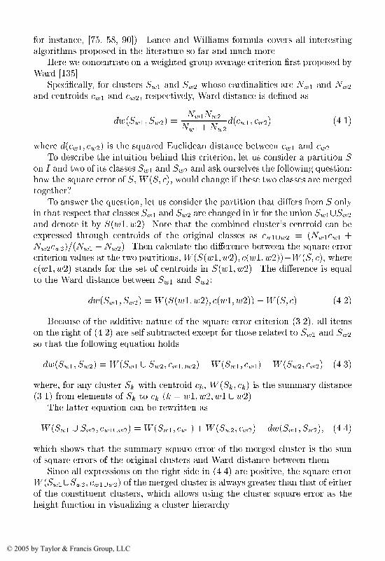
��� WARD HIERARCHICAL CLUSTERING
for instance� ���� ��� ����� Lance and Williams formula covers all interestingalgorithms proposed in the literature so far and much more�Here we concentrate on a weighted group average criterion rst proposed by
Ward ������Specically� for clusters Sw� and Sw� whose cardinalities are Nw� and Nw�
and centroids cw� and cw�� respectively� Ward distance is dened as
dw�Sw�� Sw�� �Nw�Nw�
Nw� !Nw�d�cw�� cw�� �����
where d�cw�� cw�� is the squared Euclidean distance between cw� and cw��To describe the intuition behind this criterion� let us consider a partition S
on I and two of its classes Sw� and Sw� and ask ourselves the following question�how the square error of S�W �S� c�� would change if these two classes are mergedtogether�To answer the question� let us consider the partition that di ers from S only
in that respect that classes Sw� and Sw� are changed in it for the union Sw��Sw�and denote it by S�w�� w��� Note that the combined cluster�s centroid can beexpressed through centroids of the original classes as cw��w� � �Nw�cw� !Nw�cw����Nw� !Nw��� Then calculate the di erence between the square errorcriterion values at the two partitions�W �S�w�� w��� c�w�� w����W �S� c�� wherec�w�� w�� stands for the set of centroids in S�w�� w��� The di erence is equalto the Ward distance between Sw� and Sw��
dw�Sw�� Sw�� �W �S�w�� w��� c�w�� w��� �W �S� c� �����
Because of the additive nature of the square error criterion ������ all itemson the right of ����� are self subtracted except for those related to Sw� and Sw�so that the following equation holds
dw�Sw�� Sw�� �W �Sw� � Sw�� cw��w���W �Sw�� cw���W �Sw�� cw�� �����
where� for any cluster Sk with centroid ck� W �Sk� ck� is the summary distance����� from elements of Sk to ck �k � w�� w�� w� � w���The latter equation can be rewritten as
W �Sw� � Sw�� cw��w�� �W �Sw�� cw�� !W �Sw�� cw�� ! dw�Sw�� Sw��� �����
which shows that the summary square error of the merged cluster is the sumof square errors of the original clusters and Ward distance between them�Since all expressions on the right side in ����� are positive� the square error
W �Sw��Sw�� cw��w�� of the merged cluster is always greater than that of eitherof the constituent clusters� which allows using the cluster square error as theheight function in visualizing a cluster hierarchy�
© 2005 by Taylor & Francis Group, LLC
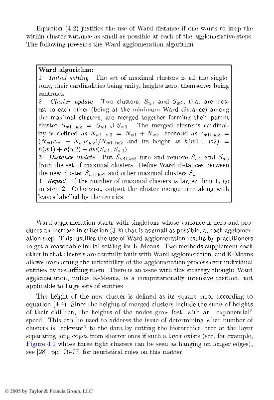
���� AGGLOMERATION� WARD ALGORITHM ���
Equation ����� justies the use of Ward distance if one wants to keep thewithin cluster variance as small as possible at each of the agglomerative steps�The following presents the Ward agglomeration algorithm�
Ward algorithm��� Initial setting� The set of maximal clusters is all the singletons� their cardinalities being unity� heights zero� themselves beingcentroids��� Cluster update� Two clusters� Sw� and Sw�� that are closest to each other �being at the minimum Ward distance� amongthe maximal clusters� are merged together forming their parentcluster Sw��w� � Sw� � Sw�� The merged cluster�s cardinality is dened as Nw��w� � Nw� ! Nw�� centroid as cw��w� ��Nw�cw� ! Nw�cw���Nw��w� and its height as h�w� � w�� �h�w�� ! h�w�� ! dw�Sw�� Sw����� Distance update� Put Sw��w� into and remove Sw� and Sw�from the set of maximal clusters� Dene Ward distances betweenthe new cluster Sw��w� and other maximal clusters St��� Repeat� If the number of maximal clusters is larger than �� goto step �� Otherwise� output the cluster merger tree along withleaves labelled by the entities�
Ward agglomeration starts with singletons whose variance is zero and produces an increase in criterion ����� that is as small as possible� at each agglomeration step� This justies the use of Ward agglomeration results by practitionersto get a reasonable initial setting for KMeans� Two methods supplement eachother in that clusters are carefully built with Ward agglomeration� and KMeansallows overcoming the in�exibility of the agglomeration process over individualentities by reshu$ing them� There is an issue with this strategy though� Wardagglomeration� unlike KMeans� is a computationally intensive method� notapplicable to large sets of entities�
The height of the new cluster is dened as its square error according toequation ������ Since the heights of merged clusters include the sums of heightsof their children� the heights of the nodes grow fast� with an �exponential�speed� This can be used to address the issue of determining what number ofclusters is �relevant� to the data by cutting the hierarchical tree at the layerseparating long edges from shorter ones if such a layer exists �see� for example�Figure ��� whose three tight clusters can be seen as hanging on longer edges��see ����� pp� ����� for heuristical rules on this matter�
© 2005 by Taylor & Francis Group, LLC
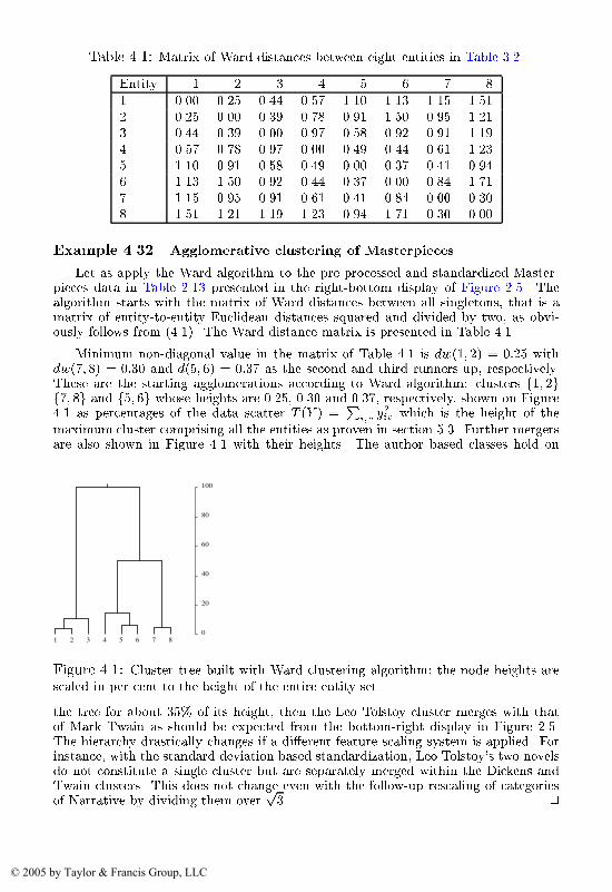
��� WARD HIERARCHICAL CLUSTERING
Table ���� Matrix of Ward distances between eight entities in Table ����
Entity � � � � � � � �
� � ��� ��� ��� ��� ���� ���� ����� ��� � ��� ��� ��� ��� ��� ����� ��� ��� � ��� ��� ��� ��� ����� ��� ��� ��� � ��� ��� ��� ����� ��� ��� ��� ��� � ��� ��� ���� ���� ��� ��� ��� ��� � ��� ����� ���� ��� ��� ��� ��� ��� � ��� ���� ���� ���� ���� ��� ���� �� �
Example ����� Agglomerative clustering of Masterpieces
Let as apply the Ward algorithm to the pre�processed and standardized Master�pieces data in Table ���� presented in the right�bottom display of Figure ���� Thealgorithm starts with the matrix of Ward distances between all singletons that is amatrix of entity�to�entity Euclidean distances squared and divided by two as obvi�ously follows from ���� � The Ward distance matrix is presented in Table ����
Minimum non�diagonal value in the matrix of Table ��� is dw��� � � ��� withdw��� � � �� and d��� � � ��� as the second and third runners�up respectively�These are the starting agglomerations according to Ward algorithm� clusters f�� �gf�� �g and f�� �g whose heights are ��� �� and ��� respectively shown on Figure��� as percentages of the data scatter T �Y �
Pi�v y
�iv which is the height of the
maximum cluster comprising all the entities as proven in section ���� Further mergersare also shown in Figure ��� with their heights� The author based classes hold on
1 2 3 4 5 6 7 80
20
40
60
80
100
Figure ���� Cluster tree built with Ward clustering algorithm� the node heights arescaled in per cent to the height of the entire entity set�
the tree for about ��� of its height then the Leo Tolstoy cluster merges with thatof Mark Twain as should be expected from the bottom�right display in Figure ����The hierarchy drastically changes if a di�erent feature scaling system is applied� Forinstance with the standard deviation based standardization Leo Tolstoy�s two novelsdo not constitute a single cluster but are separately merged within the Dickens andTwain clusters� This does not change even with the follow�up rescaling of categoriesof Narrative by dividing them over
p�� �
© 2005 by Taylor & Francis Group, LLC
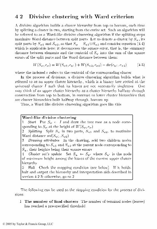
���� DIVISIVE CLUSTERING WITH WARD CRITERION ���
��� Divisive clustering with Ward criterion
A divisive algorithm builds a cluster hierarchy from top to bottom� each timeby splitting a cluster in two� starting from the entire set� Such an algorithm willbe referred to as a Wardlike divisive clustering algorithm if the splitting stepsmaximize Ward distance between split parts� Let us denote a cluster by Sw� itssplit parts by Sw� and Sw�� so that Sw � Sw��Sw� and consider equation �����which is applicable here� it decomposes the square error� that is� the summarydistance between elements and the centroid of Sw into the sum of the squareerrors of the split parts and the Ward distance between them�
W �Sw� cw� �W �Sw�� cw�� !W �Sw�� cw�� ! dw�cw�� cw�� �����
where the indexed c refers to the centroid of the corresponding cluster�In the process of divisions� a divisive clustering algorithm builds what is
referred to as an upper cluster hierarchy� which is a binary tree rooted at theuniversal cluster I such that its leaves are not necessarily singletons� Onemay think of an upper cluster hierarchy as a cluster hierarchy halfway throughconstruction from top to bottom� in contrast to lower cluster hierarchies thatare cluster hierarchies built halfway through� bottom up�Thus� a Wardlike divisive clustering algorithm goes like this�
Ward�like divisive clustering�� Start� Put Sw � I and draw the tree root as a node corresponding to Sw at the height of W �Sw� cw���� Splitting� Split Sw in two parts� Sw� and Sw�� to maximizeWard distance wd�Sw�� Sw����� Drawing attributes� In the drawing� add two children nodescorresponding to Sw� and Sw� at the parent node corresponding toSw� their heights being their square errors��� Cluster set�s update� Set Sw � Sw� where Sw� is the nodeof maximum height among the leaves of the current upper clusterhierarchy��� Halt� Check the stopping condition �see below�� If it holds�halt and output the hierarchy and interpretation aids described insection ������ otherwise� go to ��
The following can be used as the stopping condition for the process of divisions�
�� The number of �nal clusters� The number of terminal nodes �leaves�has reached a prespecied threshold�
© 2005 by Taylor & Francis Group, LLC
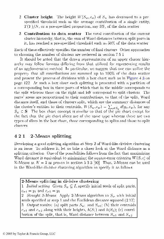
��� WARD HIERARCHICAL CLUSTERING
�� Cluster height� The height W �Sw� cw� of Sw has decreased to a prespecied threshold such as the average contribution of a single entity�T �Y ��N � or a prespecied proportion� say � � of the data scatter�
�� Contribution to data scatter� The total contribution of the currentcluster hierarchy� that is� the sum of Ward distances between split parts init� has reached a prespecied threshold such as �� of the data scatter�
Each of these e ectively species the number of nal clusters� Other approachesto choosing the number of clusters are reviewed in section ������It should be noted that the drawn representation of an upper cluster hier
archy may follow formats di ering from that utilized for representing resultsof an agglomerative method� In particular� we suggest that one can utilize theproperty that all contributions are summed up to ��� of the data scatterand present the process of divisions with a box chart such as in Figure ��� onpage ���� At such a box chart each splitting is presented with a partition ofa corresponding box in three parts of which that in the middle corresponds tothe split whereas those on the right and left correspond to split clusters� Theparts� areas are proportional to their contributions� to that of the split� Warddistance itself� and those of clusters split� which are the summary distances ofthe cluster�s entities to their centroids� W �Sw� cw� �
Pi�Sw
d�yi� cw�� for anySw � S� The box chart concept is similar to that of the pie chart except forthe fact that the pie chart slices are of the same type whereas there are twotypes of slices in the box chart� those corresponding to splits and those to splitclusters�
����� �Means splitting
Developing a good splitting algorithm at Step � of Wardlike divisive clusteringis an issue� To address it� let us take a closer look at the Ward distance as asplitting criterion� One of the possibilities follows from the fact that maximizingWard distance is equivalent to minimizing the squareerror criterion W �S� c� ofKMeans at K � � as proven in section ����� ����� Thus� �Means can be usedin the Wardlike divisive clustering algorithm to specify it as follows�
��Means splitting in divisive clustering�� Initial setting� Given Sw � I � specify initial seeds of split parts�cw� � y� and cw� � y���� Straight ��Means� Apply �Means algorithm to Sw with initialseeds specied at step � and the Euclidean distance squared ��������� Output results� �a� split parts Sw� and Sw�� �b� their centroidscw� and cw� along with their heights� h�S�� and h�S��� �c� contribution of the split� that is� Ward distance between Sw� and Sw��
© 2005 by Taylor & Francis Group, LLC
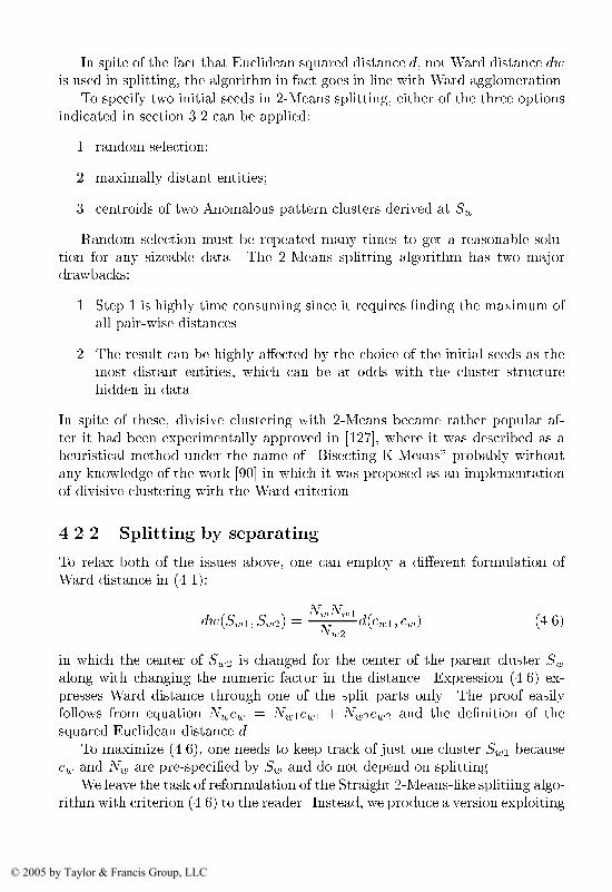
���� DIVISIVE CLUSTERING WITH WARD CRITERION ���
In spite of the fact that Euclidean squared distance d� not Ward distance dwis used in splitting� the algorithm in fact goes in line with Ward agglomeration�To specify two initial seeds in �Means splitting� either of the three options
indicated in section ��� can be applied�
�� random selection�
�� maximally distant entities�
�� centroids of two Anomalous pattern clusters derived at Sw�
Random selection must be repeated many times to get a reasonable solution for any sizeable data� The �Means splitting algorithm has two majordrawbacks�
�� Step � is highly time consuming since it requires nding the maximum ofall pairwise distances�
�� The result can be highly a ected by the choice of the initial seeds as themost distant entities� which can be at odds with the cluster structurehidden in data�
In spite of these� divisive clustering with �Means became rather popular after it had been experimentally approved in ������ where it was described as aheuristical method under the name of �Bisecting KMeans� probably withoutany knowledge of the work ���� in which it was proposed as an implementationof divisive clustering with the Ward criterion�
����� Splitting by separating
To relax both of the issues above� one can employ a di erent formulation ofWard distance in ������
dw�Sw�� Sw�� �NwNw�
Nw�d�cw�� cw� �����
in which the center of Sw� is changed for the center of the parent cluster Swalong with changing the numeric factor in the distance� Expression ����� expresses Ward distance through one of the split parts only� The proof easilyfollows from equation Nwcw � Nw�cw� ! Nw�cw� and the denition of thesquared Euclidean distance d�To maximize ������ one needs to keep track of just one cluster Sw� because
cw and Nw are prespecied by Sw and do not depend on splitting�We leave the task of reformulation of the Straight �Meanslike splitiing algo
rithm with criterion ����� to the reader� Instead� we produce a version exploiting
© 2005 by Taylor & Francis Group, LLC
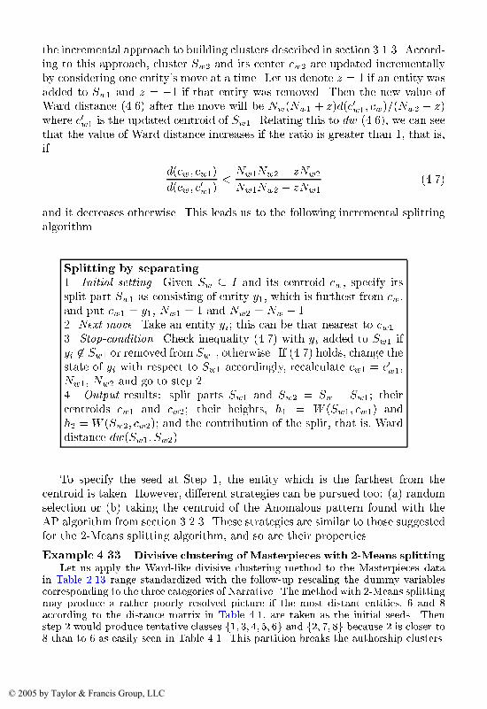
��� WARD HIERARCHICAL CLUSTERING
the incremental approach to building clusters described in section ������ According to this approach� cluster Sw� and its center cw� are updated incrementallyby considering one entity�s move at a time� Let us denote z � � if an entity wasadded to Sw� and z � �� if that entity was removed� Then the new value ofWard distance ����� after the move will be Nw�Nw� ! z�d�c�w�� cw���Nw� � z�where c�w� is the updated centroid of Sw�� Relating this to dw ������ we can seethat the value of Ward distance increases if the ratio is greater than �� that is�if
d�cw� cw��
d�cw� c�w���Nw�Nw� ! zNw�
Nw�Nw� � zNw������
and it decreases otherwise� This leads us to the following incremental splittingalgorithm�
Splitting by separating�� Initial setting� Given Sw � I and its centroid cw� specify itssplit part Sw� as consisting of entity y�� which is furthest from cw�and put cw� � y�� Nw� � � and Nw� � Nw � ���� Next move� Take an entity yi� this can be that nearest to cw���� Stop�condition� Check inequality ����� with yi added to Sw� ifyi � Sw� or removed from Sw�� otherwise� If ����� holds� change thestate of yi with respect to Sw� accordingly� recalculate cw� � c�w��Nw�� Nw� and go to step ���� Output results� split parts Sw� and Sw� � Sw � Sw�� theircentroids cw� and cw�� their heights� h� � W �Sw�� cw�� andh� �W �Sw�� cw��� and the contribution of the split� that is� Warddistance dw�Sw�� Sw���
To specify the seed at Step �� the entity which is the farthest from thecentroid is taken� However� di erent strategies can be pursued too� �a� randomselection or �b� taking the centroid of the Anomalous pattern found with theAP algorithm from section ������ These strategies are similar to those suggestedfor the �Means splitting algorithm� and so are their properties�
Example ����� Divisive clustering of Masterpieces with � Means splitting
Let us apply the Ward�like divisive clustering method to the Masterpieces datain Table ���� range standardized with the follow�up rescaling the dummy variablescorresponding to the three categories of Narrative� The method with ��Means splittingmay produce a rather poorly resolved picture if the most distant entities � and �according to the distance matrix in Table ��� are taken as the initial seeds� Thenstep � would produce tentative classes f�� �� �� �� �g and f�� �� �g because � is closer to� than to � as easily seen in Table ���� This partition breaks the authorship clusters�
© 2005 by Taylor & Francis Group, LLC
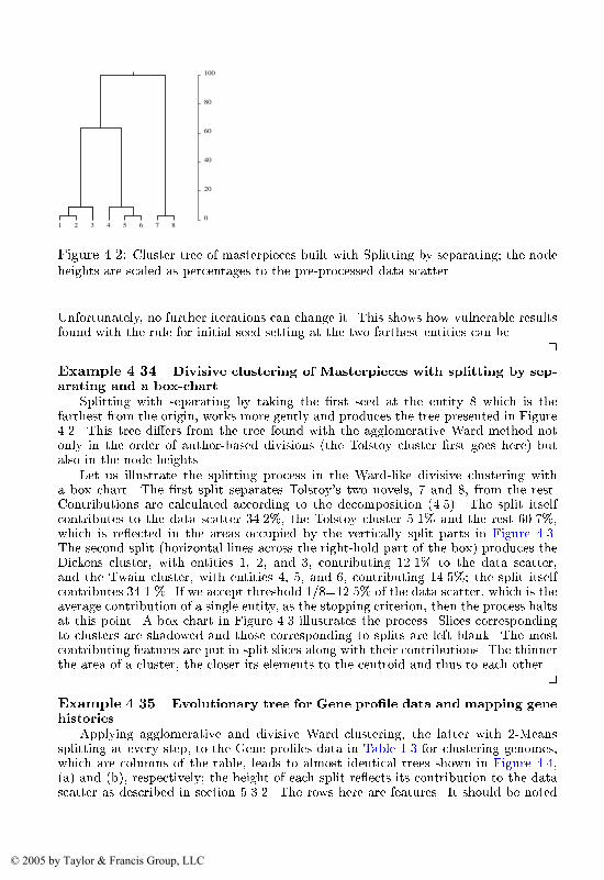
���� DIVISIVE CLUSTERING WITH WARD CRITERION ���
1 2 3 4 5 6 7 80
20
40
60
80
100
Figure ���� Cluster tree of masterpieces built with Splitting by separating� the nodeheights are scaled as percentages to the pre�processed data scatter�
Unfortunately no further iterations can change it� This shows how vulnerable resultsfound with the rule for initial seed setting at the two farthest entities can be�
�
Example ����� Divisive clustering of Masterpieces with splitting by sep arating and a box chart
Splitting with separating by taking the �rst seed at the entity � which is thefarthest from the origin works more gently and produces the tree presented in Figure���� This tree di�ers from the tree found with the agglomerative Ward method notonly in the order of author�based divisions �the Tolstoy cluster �rst goes here butalso in the node heights�
Let us illustrate the splitting process in the Ward�like divisive clustering witha box chart� The �rst split separates Tolstoy�s two novels � and � from the rest�Contributions are calculated according to the decomposition ���� � The split itselfcontributes to the data scatter ����� the Tolstoy cluster ���� and the rest ����which is re"ected in the areas occupied by the vertically split parts in Figure ����The second split �horizontal lines across the right�hold part of the box produces theDickens cluster with entities � � and � contributing ����� to the data scatterand the Twain cluster with entities � � and � contributing ������ the split itselfcontributes ���� �� If we accept threshold ��������� of the data scatter which is theaverage contribution of a single entity as the stopping criterion then the process haltsat this point� A box chart in Figure ��� illustrates the process� Slices correspondingto clusters are shadowed and those corresponding to splits are left blank� The mostcontributing features are put in split slices along with their contributions� The thinnerthe area of a cluster the closer its elements to the centroid and thus to each other�
�
Example ����� Evolutionary tree for Gene pro�le data and mapping genehistories
Applying agglomerative and divisive Ward clustering the latter with ��Meanssplitting at every step to the Gene pro�les data in Table ��� for clustering genomeswhich are columns of the table leads to almost identical trees shown in Figure ����a and �b respectively� the height of each split re"ects its contribution to the datascatter as described in section ������ The rows here are features� It should be noted
© 2005 by Taylor & Francis Group, LLC
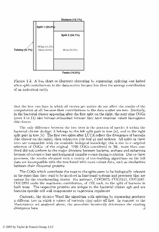
��� WARD HIERARCHICAL CLUSTERING
SCon (25.2%)
Twain (14.5%)
Tolstoy (5.1%)
Dickens (12.1%)
Split 2 (34.1%)
Split 1 (34.2%)
Direct (8.4%)NChar (11.2%)
Figure ���� A box chart to illustrate clustering by separating� splitting was haltedwhen split contributions to the data scatter became less than the average contributionof an individual entity�
that the �rst two lines in which all entries are unities do not a�ect the results of thecomputation at all because their contributions to the data scatter are zero� Similarlyin the bacterial cluster appearing after the �rst split on the right the next nine COGs�rows � to �� also become redundant because they have constant values throughoutthis cluster�
The only di�erence between the two trees is the position of species b within thebacterial cluster dcrbjqv� b belongs to the left split part in tree �a and to the rightsplit part in tree �b � The �rst two splits after LUCA re"ect the divergence of bacteria�the cluster on the right then eukaryota �the leaf y and archaea� All splits in thesetrees are compatible with the available biological knowledge� this is due to a targetedselection of COGs� of the original �� COGs considered in #��$ more than one�third did not conform to the major divisions between bacteria archaea and eukaryotabecause of extensive loss and horizontal transfer events during evolution� Due to theseprocesses the results obtained with a variety of tree�building algorithms on the fulldata are incompatible with the tree found with more robust data such as similaritiesbetween their ribosomal proteins�
The COGs which contribute the most to the splits seem to be biologically relevantin the sense that they tend to be involved in functional systems and processes that areunique for the corresponding cluster� For instance COG��� COG���� COG���COG���� make the maximum contribution of ��� each to the split of bacteria inboth trees� The respective proteins are unique to the bacterial cluster egfs and arebacteria�speci�c cell wall components or expression regulators�
Curiously the divisive Ward�like algorithm with splitting by separating producesa di�erent tree in which a subset of bacteria efgsj splits o� �rst� In contrast to theMasterpieces set analyzed above the procedure incorrectly determines the startingdivergence here� �
© 2005 by Taylor & Francis Group, LLC
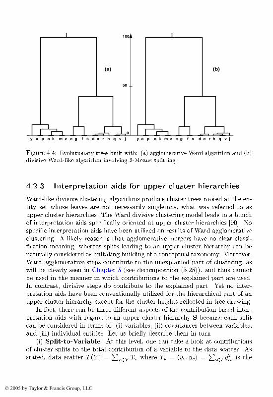
���� DIVISIVE CLUSTERING WITH WARD CRITERION ���
100
50
0
(a) (b)
y a p o k m z e g f s d c r h q v j y a p o k m z e g f s d c r h q v j
Figure ���� Evolutionary trees built with� �a agglomerative Ward algorithm and �b divisive Ward�like algorithm involving ��Means splitting�
����� Interpretation aids for upper cluster hierarchies
Wardlike divisive clustering algorithms produce cluster trees rooted at the entity set whose leaves are not necessarily singletons� what was referred to asupper cluster hierarchies� The Ward divisive clustering model leads to a bunchof interpretation aids specically oriented at upper cluster hierarchies ����� Nospecic interpretation aids have been utilized on results of Ward agglomerativeclustering� A likely reason is that agglomerative mergers have no clear classication meaning� whereas splits leading to an upper cluster hierarchy can benaturally considered as imitating building of a conceptual taxonomy� Moreover�Ward agglomerative steps contribute to the unexplained part of clustering� aswill be clearly seen in Chapter � �see decomposition �������� and thus cannotbe used in the manner in which contributions to the explained part are used�In contrast� divisive steps do contribute to the explained part� Yet no interpretation aids have been conventionally utilized for the hierarchical part of anupper cluster hierarchy except for the cluster heights re�ected in tree drawing�In fact� there can be three di erent aspects of the contribution based inter
pretation aids with regard to an upper cluster hierarchy S because each splitcan be considered in terms of� �i� variables� �ii� covariances between variables�and �iii� individual entities� Let us brie�y describe them in turn��i� Split�to�Variable� At this level� one can take a look at contributions
of cluster splits to the total contribution of a variable to the data scatter� Asstated� data scatter T �Y � �
Pv�V Tv where Tv � �yv� yv� �
Pi�I y
�iv is the
© 2005 by Taylor & Francis Group, LLC
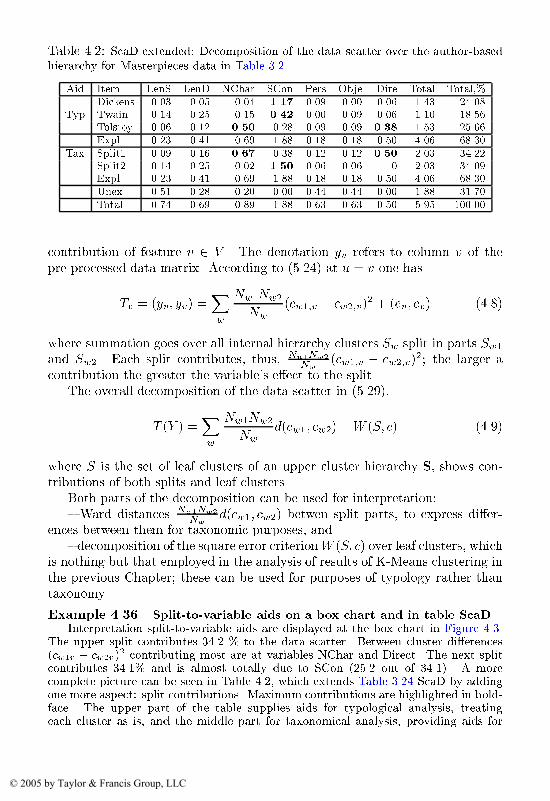
��� WARD HIERARCHICAL CLUSTERING
Table ���� ScaD extended� Decomposition of the data scatter over the author�basedhierarchy for Masterpieces data in Table ����
Aid Item LenS LenD NChar SCon Pers Obje Dire Total Total��Dickens ���� ���� ��� ���� ��� ���� ���� ��� ����
Typ Twain ��� ���� ���� ���� ���� ��� ���� ���� �����Tolstoy ���� ���� ���� ���� ��� ��� ��� ���� �����Expl ���� ��� ��� ���� ���� ���� ���� ��� �����
Tax Split� ��� ���� ��� ���� ���� ���� ���� ���� ����Split� ��� ���� ���� ���� ���� ���� � ���� ���Expl ���� ��� ��� ���� ���� ���� ���� ��� �����Unex ���� ���� ���� ���� �� �� ���� ���� �����Total ��� ��� ��� ���� ���� ���� ���� ��� ������
contribution of feature v � V � The denotation yv refers to column v of thepreprocessed data matrix� According to ������ at u � v one has
Tv � �yv� yv� �Xw
Nw�Nw�
Nw�cw��v � cw��v�
� ! �ev � ev� �����
where summation goes over all internal hierarchy clusters Sw split in parts Sw�and Sw�� Each split contributes� thus�
Nw�Nw�
Nw�cw��v � cw��v�
�� the larger acontribution the greater the variable�s e ect to the split�The overall decomposition of the data scatter in �������
T �Y � �Xw
Nw�Nw�
Nwd�cw�� cw�� !W �S� c� �����
where S is the set of leaf clusters of an upper cluster hierarchy S� shows contributions of both splits and leaf clusters�Both parts of the decomposition can be used for interpretation�� Ward distances Nw�Nw�
Nwd�cw�� cw�� betwen split parts� to express di er
ences between them for taxonomic purposes� and� decomposition of the square error criterionW �S� c� over leaf clusters� which
is nothing but that employed in the analysis of results of KMeans clustering inthe previous Chapter� these can be used for purposes of typology rather thantaxonomy�
Example ����� Split to variable aids on a box chart and in table ScaDInterpretation split�to�variable aids are displayed at the box chart in Figure ����
The upper split contributes ���� � to the data scatter� Between cluster di�erences�cw�v � cw�v � contributing most are at variables NChar and Direct� The next splitcontributes ����� and is almost totally due to SCon ����� out of ���� � A morecomplete picture can be seen in Table ��� which extends Table ���� ScaD by addingone more aspect� split contributions� Maximum contributions are highlighted in bold�face� The upper part of the table supplies aids for typological analysis treatingeach cluster as is and the middle part for taxonomical analysis providing aids for
© 2005 by Taylor & Francis Group, LLC
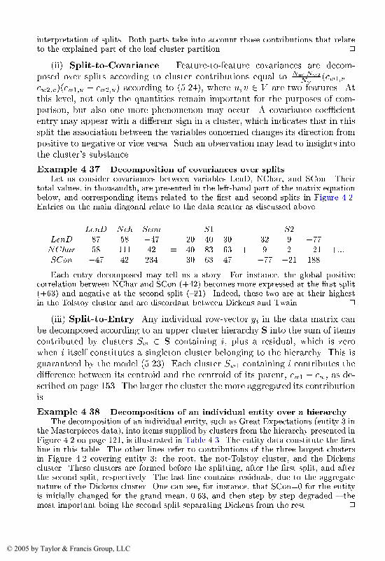
���� DIVISIVE CLUSTERING WITH WARD CRITERION ���
interpretation of splits� Both parts take into account those contributions that relateto the explained part of the leaf cluster partition� �
�ii� Split�to�Covariance� Featuretofeature covariances are decomposed over splits according to cluster contributions equal to Nw�Nw�
Nw�cw��v �
cw��v��cw��u � cw��u� according to ������� where u� v � V are two features� Atthis level� not only the quantities remain important for the purposes of comparison� but also one more phenomenon may occur� A covariance coe�ciententry may appear with a di erent sign in a cluster� which indicates that in thissplit the association between the variables concerned changes its direction frompositive to negative or vice versa� Such an observation may lead to insights intothe cluster�s substance�
Example ����� Decomposition of covariances over splitsLet us consider covariances between variables LenD NChar and SCon� Their
total values in thousandth are presented in the left�hand part of the matrix equationbelow and corresponding items related to the �rst and second splits in Figure ����Entries on the main diagonal relate to the data scatter as discussed above�
LenD Nch Scon S� S�LenD �� �� ��� � � � �� � ���NChar �� ��� �� � � �� �� � � � ��� ����SCon ��� �� ��� � �� �� ��� ��� ���
Each entry decomposed may tell us a story� For instance the global positivecorrelation between NChar and SCon ���� becomes more expressed at the �rst split���� and negative at the second split ���� � Indeed these two are at their highestin the Tolstoy cluster and are discordant between Dickens and Twain� �
�iii� Split�to�Entry� Any individual rowvector yi in the data matrix canbe decomposed according to an upper cluster hierarchy S into the sum of itemscontributed by clusters Sw � S containing i� plus a residual� which is zerowhen i itself constitutes a singleton cluster belonging to the hierarchy� This isguaranteed by the model ������� Each cluster Sw� containing i contributes thedi erence between its centroid and the centroid of its parent� cw� � cw� as described on page ���� The larger the cluster the more aggregated its contributionis�
Example ����� Decomposition of an individual entity over a hierarchyThe decomposition of an individual entity such as Great Expectations �entity � in
the Masterpieces data into items supplied by clusters from the hierarchy presented inFigure ��� on page ��� is illustrated in Table ���� The entity data constitute the �rstline in this table� The other lines refer to contributions of the three largest clustersin Figure ��� covering entity �� the root the not�Tolstoy cluster and the Dickenscluster� These clusters are formed before the splitting after the �rst split and afterthe second split respectively� The last line contains residuals due to the aggregatenature of the Dickens cluster� One can see for instance that SCon� for the entityis initially changed for the grand mean ��� and then step by step degraded � themost important being the second split separating Dickens from the rest� �
© 2005 by Taylor & Francis Group, LLC
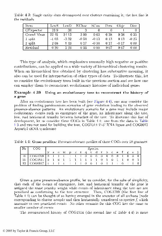
��� WARD HIERARCHICAL CLUSTERING
Table ���� Single entity data decomposed over clusters containing it� the last line isthe residuals�
Item LenS LenD NChar SCon Pers Obje Dire
GExpectat ���� �� � �
Grand Mean ����� ����� �� ��� ��� ��� ���� split ���� ����� ��� ���� ��� ��� ����� split ���� ���� ��� ��� ��� ���� �
Residual ��� ����� ��� � ���� ��� �
This type of analysis� which emphasizes unusually high negative or positivecontributions� can be applied to a wide variety of hierarchical clustering results�When an hierarchical tree obtained by clustering has substantive meaning� italso can be used for interpretation of other types of data� To illustrate this� letus consider the evolutionary trees built in the previous section and see how onecan employ them to reconstruct evolutionary histories of individual genes�
Example ����� Using an evolutionary tree to reconstruct the history ofa gene
After an evolutionary tree has been built �see Figure ��� one may consider theproblem of �nding parsimonious scenarios of gene evolution leading to the observedpresence�absence patterns� An evolutionary scenario for a gene may include majorevolutionary events such as emergence of the gene its inheritance along the treeloss and horizontal transfer between branches of the tree� To illustrate this line ofdevelopment let us consider three COGs in Table ���� one from the data in Table��� and two not used for building the tree COG���� ����� RNA ligase and COG��Aspartyl�tRNA synthetase�
Table ���� Gene pro�les� Presence�absence pro�les of three COGs over �� genomes�
No COG Speciesy a o m p k z q v d r b c e f g s j
�� COG��� � � � � � � � � � � � � � � � � � ��� COG��� � � � � � � � � � � � � � � � � � ��� COG���� � � � � � � � � � � � � � � � � � �
Given a gene presence�absence pro�le let us consider for the sake of simplicitythat each of the events of emergence loss and horizontal transfer of the gene isassigned the same penalty weight while events of inheritance along the tree are notpenalized as conforming to the tree structure� Then COG��� �the �rst line ofTable ��� can be thought of as having emerged in the ancestor of all archaea �nodecorresponding to cluster aompkz and then horizontally transferred to species f whichamounts to two penalized events� No other scenario for this COG has the same orsmaller number of events�
The reconstructed history of COG���� �the second line of Table ��� is more
© 2005 by Taylor & Francis Group, LLC
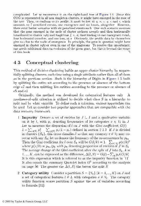
���� CONCEPTUAL CLUSTERING ���
complicated� Let us reconstruct it on the right�hand tree of Figure ���� Since thisCOG is represented in all non�singleton clusters it might have emerged in the root ofthe tree� Then to conform to its pro�le it must be lost at y� o� s� g� c and r whichamounts to � penalized events one emergence and six losses altogether� Howeverthere exist better scenarios with six penalized events each� One such scenario assumesthat the gene emerged in the node of cluster archaea aompkz and then horizontallytransferred to cluster vqbj and singletons f� e� d thus leading to one emergence eventfour horizontal transfers and one loss at o� Obviously the pro�le data by themselvesgive no clue to the node of emergence� In principle the gene in question might haveemerged in cluster vqbj or even in one of the singletons� To resolve this uncertaintyone needs additional data on evolution of the given gene but this is beyond the scopeof this book� �
��� Conceptual clustering
This method of divisive clustering builds an upper cluster hierarchy by sequentially splitting clusters� each time using a single attribute rather than all of themas in the previous section� Such is the hierarchy of Digits in Figure ��� builtby splitting the entire set according to the presence or absence of the bottomedge e� and then splitting Yes entities according to the presence or absence ofe� and e��Originally� the method was developed for categorical features only� A
goodnessofsplit criterion is utilized to decide what class S in a hierarchy tosplit and by what variable� To dene such a criterion� various approaches canbe used� Let us consider two popular approaches that are compatible with thedata recovery framework�
�� Impurity� Denote a set of entities by J � I and a qualitative variableon it by l� with pv denoting frequencies of its categories v � Vl in J �Let us measure the dispersion of l on J with the Gini coe�cient� G�l� ���Pv�Vl
p�v �P
v�Vlpv��� pv� dened in section ������ If J is divided
in clusters fSkg� this cross classies l so that any category v � Vl may cooccur with any Sk� let us denote the frequency of the cooccurrence by pkv �Then the Gini coe�cient for l over Sk will be G�l�k� � ��
Pv�Vl
p�v�k��
where p�v�k� � pkv�pk with pk denoting proportion of entities of J in Sk�The average change of the Gini coe�cient after the split of J into Sk� k ��� ����K� can be expressed as the di erence� %�l� S� � G�l��Pk pkG�l�k��It is this expression which is referred to as the impurity function in �����It also equals the summary Quetelet index G� according to the analysison page ��� The greater the %�l� S� the better the split S�
�� Category utility� Consider a partition S � fSkg �k � �� ����K� on J anda set of categorical features l � L with categories v � Vl� The categoryutility function scores partition S against the set of variables accordingto formula �����
© 2005 by Taylor & Francis Group, LLC
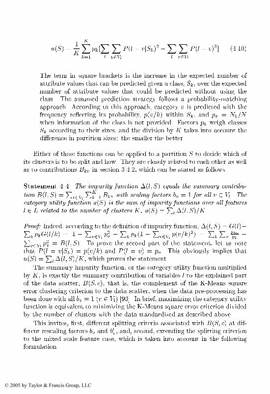
��� WARD HIERARCHICAL CLUSTERING
u�S� ��
K
KXk��
pk�Xl
Xv�Vl
P �l � vjSk�� �Xl
Xv�Vl
P �l � v��� ������
The term in square brackets is the increase in the expected number ofattribute values that can be predicted given a class� Sk� over the expectednumber of attribute values that could be predicted without using theclass� The assumed prediction strategy follows a probabilitymatchingapproach� According to this approach� category v is predicted with thefrequency re�ecting its probability� p�v�k� within Sk� and pk � Nk�Nwhen information of the class is not provided� Factors pk weigh classesSk according to their sizes� and the division by K takes into account thedi erence in partition sizes� the smaller the better�
Either of these functions can be applied to a partition S to decide which ofits clusters is to be split and how� They are closely related to each other as wellas to contributions Bkv in section ������ which can be stated as follows�
Statement ���� The impurity function %�l� S� equals the summary contribu�
tion B�l� S� �P
v�Vl
PKk�� Bkv with scaling factors bv � � for all v � Vl� The
category utility function u�S� is the sum of impurity functions over all featuresl � L related to the number of clusters K� u�S� �
Pl%�l� S��K�
Proof� Indeed� according to the denition of impurity function� %�l� S� � G�l��Pk pkG�l�k� � � � Pv�Vl
p�v �P
k pk�� �P
v�Vlp�v�k��� �
Pk
Pvpkvpk
�Pv�Vl
p�v � B�l� S�� To prove the second part of the statement� let us notethat P �l � vjSk� � p�v�k� and P �l � v� � pv� This obviously implies thatu�S� �
Pl%�l� S��K� which proves the statement�
The summary impurity function� or the category utility function multipliedby K� is exactly the summary contribution of variables l to the explained partof the data scatter� B�S� c�� that is� the complement of the KMeans squareerror clustering criterion to the data scatter� when the data preprocessing hasbeen done with all bv � � �v � Vl� ����� In brief� maximizing the category utilityfunction is equivalent to minimizing the KMeans square error criterion dividedby the number of clusters with the data standardized as described above�
This invites� rst� di erent splitting criteria associated with B�S� c� at different rescaling factors bv and b
�v� and� second� extending the splitting criterion
to the mixed scale feature case� which is taken into account in the followingformulation�
© 2005 by Taylor & Francis Group, LLC
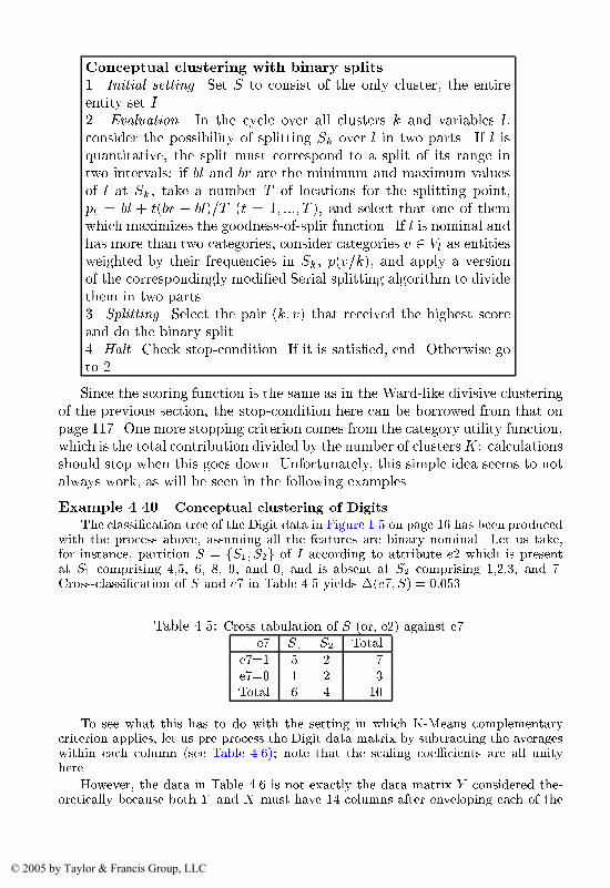
���� CONCEPTUAL CLUSTERING ���
Conceptual clustering with binary splits�� Initial setting� Set S to consist of the only cluster� the entireentity set I ��� Evaluation� In the cycle over all clusters k and variables l�consider the possibility of splitting Sk over l in two parts� If l isquantitative� the split must correspond to a split of its range intwo intervals� if bl and br are the minimum and maximum valuesof l at Sk� take a number T of locations for the splitting point�pt � bl ! t�br � bl��T �t � �� ���� T �� and select that one of themwhich maximizes the goodnessofsplit function� If l is nominal andhas more than two categories� consider categories v � Vl as entitiesweighted by their frequencies in Sk� p�v�k�� and apply a versionof the correspondingly modied Serial splitting algorithm to dividethem in two parts��� Splitting� Select the pair �k� v� that received the highest scoreand do the binary split��� Halt� Check stopcondition� If it is satised� end� Otherwise goto ��
Since the scoring function is the same as in the Wardlike divisive clusteringof the previous section� the stopcondition here can be borrowed from that onpage ���� One more stopping criterion comes from the category utility function�which is the total contribution divided by the number of clustersK� calculationsshould stop when this goes down� Unfortunately� this simple idea seems to notalways work� as will be seen in the following examples�
Example ���� Conceptual clustering of Digits
The classi�cation tree of the Digit data in Figure ��� on page �� has been producedwith the process above assuming all the features are binary nominal� Let us takefor instance partition S � fS�� S�g of I according to attribute e� which is presentat S� comprising �� � � � and and is absent at S� comprising ��� and ��Cross�classi�cation of S and e� in Table ��� yields %�e�� S � ����
Table ���� Cross�tabulation of S �or e� against e��
e� S� S� Total
e��� � � �e�� � � �Total � � �
To see what this has to do with the setting in which K�Means complementarycriterion applies let us pre�process the Digit data matrix by subtracting the averageswithin each column �see Table ��� � note that the scaling coe�cients are all unityhere�
However the data in Table ��� is not exactly the data matrix Y considered the�oretically because both Y and X must have �� columns after enveloping each of the
© 2005 by Taylor & Francis Group, LLC
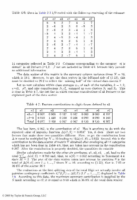
��� WARD HIERARCHICAL CLUSTERING
Table ���� Data in Table ��� �� coded with the follow�up centering of the columns�
e� e� e� e� e� e� e�
��� ��� �� ��� ��� �� ����� ��� �� �� �� ��� ���� ��� �� �� ��� �� ��
��� �� �� �� ��� �� ����� �� ��� �� ��� �� ���� �� ��� �� �� �� ���� ��� �� ��� ��� �� ����� �� �� �� �� �� ���� �� �� �� ��� �� ���� �� �� ��� �� �� ��
�� categories re"ected in Table ���� Columns corresponding to the category �ei isabsent� in all features i������� are not included in Table ��� because they provideno additional information�
The data scatter of this matrix is the summary column variance times N � �which is ����� However to get the data scatter in the lefthand side of ����� thismust be doubled to ���� to re"ect the �missing half� of the virtual data matrix Y �
Let us now calculate within class averages ckv of each of the variables k � �� �v�e����e� and take contributions Nkc
�kv summed up over clusters S� and S�� This
is done in Table ��� the last line in which contains contributions of all features to theexplained part of the data scatter�
Table ���� Feature contributions to digit classes de�ned by e��
e� e� e� e� e� e� e� e�
e��� �� ��� ��� ��� �� �� ���e�� �� ���� ��� ��� �� �� ���Total ��� ��� ���� ���� ��� ��� ����
The last item ���� is the contribution of e�� Has it anything to do with thereported value of impurity function %�e�� S � ���� Yes it does� There are twofactors that make these two quantities di�erent� First to get the contribution from% it must be multiplied by N � � leading to �%�e�� S � ����� Second this is thecontribution to the data scatter of matrix Y obtained after enveloping all �� categorieswhich has not been done in Table ��� thus not taken into account in the contribution����� After the contribution is properly doubled the quantities do coincide�
Similar calculations made for the other six attributes e� e� e���� e� lead to thetotal
Pl� %�el� S � ��� and thus to u�S � ���� according to Statement ����
since M � �� The part of the data scatter taken into account by partition S is thetotal of %�S� el over l � �� ���� � times N � � according to ����� that is ��� or����� of the scatter �����
The evaluations at the �rst splitting step of the total Digit set actually involve allpairwise contingency coe�cients G��l� l� � %�l� l� �l� l� � �� ���� � displayed in Table���� According to this data the maximum summary contribution is supplied by theS made according to e�� it is equal to ���� which is ����� of the total data scatter�
© 2005 by Taylor & Francis Group, LLC
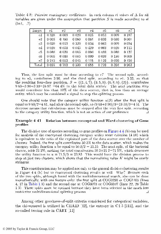
���� CONCEPTUAL CLUSTERING ���
Table ���� Pairwise contingency coe�cients� In each column el values of % for allvariables are given under the assumption that partition S is made according to el�l������ �
Target e� e� e� e� e� e� e�
e� ��� �� �� ��� ��� �� ����e� �� ��� �� ��� �� �� ���e� �� ��� ��� ��� �� �� ���e� �� ��� ��� ��� �� �� ����e� �� �� �� �� ��� �� ����e� �� �� �� �� �� ��� ��e� ���� ��� ��� ���� ��� �� ���
Total ���� ��� ��� ���� ��� ���� ����
Thus the �rst split must be done according to e�� The second split accord�ing to e� contributes ��� and the third split according to e� ���� so thatthe resulting four�class partition S � ff�� �� �g� f�� �� �g� f�� �� g� f�gg contributes������������������� ������ to the total data scatter� The next partition stepwould contribute less than �� of the data scatter that is less than an averageentity which may be considered a signal to stop the splitting process�
One should note that the category utility function u�S after the �rst split isequal to ����������� and after the second split to ��������� ���������������� Thedecrease means that calculations must be stopped after the very �rst split accordingto the category utility function which is not an action of our preference� �
Example ����� Relation between conceptual and Ward clustering of Genepro�les
The divisive tree of species according to gene pro�les on Figure ��� �b can be usedfor analysis of the conceptual clustering category utility score criterion ���� whichis equivalent to the ratio of the explained part of the data scatter over the number ofclusters� Indeed the �rst split contributes ���� to the data scatter which makes thecategory utility function u be equal to ����� � ������ The next split of the bacterialcluster adds ����� making the total contribution �������������� which decreasesthe utility function to u � ������ � ������ This would force the division process tostop at just two clusters which shows that the normalizing value K might be overlystringent�
This consideration may be applied not only to the general divisive clustering resultsin Figure ��� �b but to conceptual clustering results as well� Why� Because eachof the two splits although found with the multidimensional search also can be donemonothetically with one feature only� the �rst split at COG�� or COG��� �lines� �� in Table ��� and the second one at COG��� or COG��� �lines �� �� Table��� � These splits must be optimal because they have been selected in the much lessrestrictive multidimensional splitting process� �
Among other goodnessofsplit criteria considered for categorical variables�the chisquared is utilized in CHAID ����� the entropy in C��� ������ and thesocalled twoing rule in CART �����
© 2005 by Taylor & Francis Group, LLC
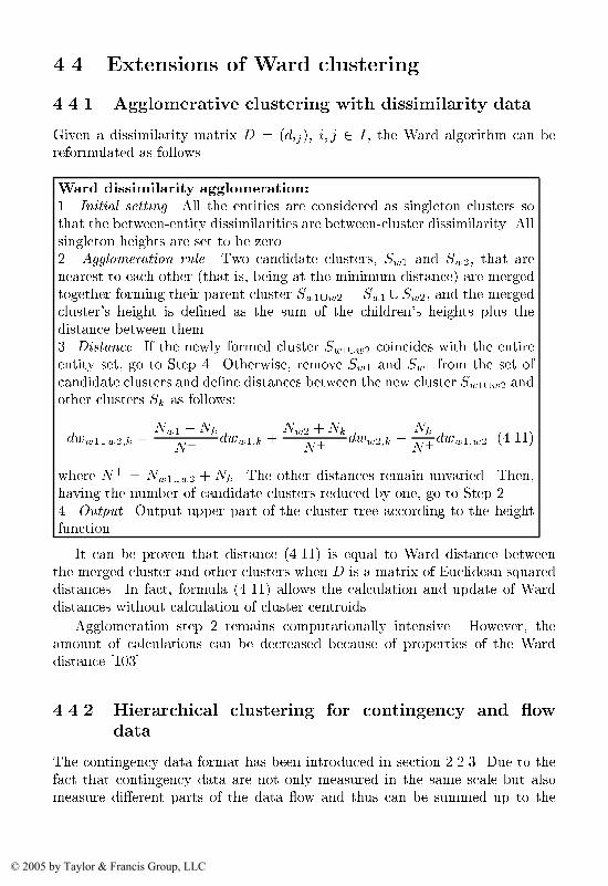
��� WARD HIERARCHICAL CLUSTERING
��� Extensions of Ward clustering
����� Agglomerative clustering with dissimilarity data
Given a dissimilarity matrix D � �dij�� i� j � I � the Ward algorithm can bereformulated as follows�
Ward dissimilarity agglomeration��� Initial setting� All the entities are considered as singleton clusters sothat the betweenentity dissimilarities are betweencluster dissimilarity� Allsingleton heights are set to be zero��� Agglomeration rule� Two candidate clusters� Sw� and Sw�� that arenearest to each other �that is� being at the minimum distance� are mergedtogether forming their parent cluster Sw��w� � Sw� �Sw�� and the mergedcluster�s height is dened as the sum of the children�s heights plus thedistance between them��� Distance� If the newly formed cluster Sw��w� coincides with the entireentity set� go to Step �� Otherwise� remove Sw� and Sw� from the set ofcandidate clusters and dene distances between the new cluster Sw��w� andother clusters Sk as follows�
dww��w��k �Nw� !Nk
N�dww��k !
Nw� !Nk
N�dww��k � Nk
N�dww��w� ������
where N� � Nw��w� ! Nk� The other distances remain unvaried� Then�having the number of candidate clusters reduced by one� go to Step ���� Output� Output upper part of the cluster tree according to the heightfunction�
It can be proven that distance ������ is equal to Ward distance betweenthe merged cluster and other clusters when D is a matrix of Euclidean squareddistances� In fact� formula ������ allows the calculation and update of Warddistances without calculation of cluster centroids�
Agglomeration step � remains computationally intensive� However� theamount of calculations can be decreased because of properties of the Warddistance ������
����� Hierarchical clustering for contingency and �owdata
The contingency data format has been introduced in section ������ Due to thefact that contingency data are not only measured in the same scale but alsomeasure di erent parts of the data �ow and thus can be summed up to the
© 2005 by Taylor & Francis Group, LLC
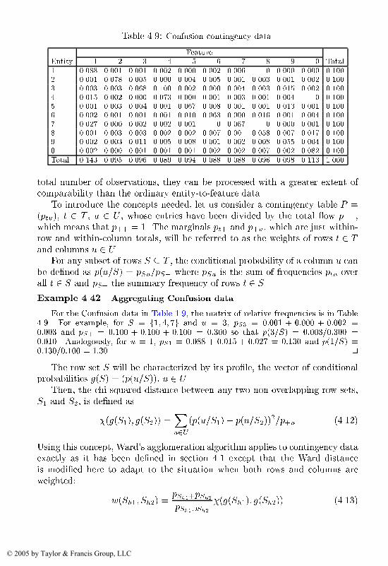
���� EXTENSIONS OF WARD CLUSTERING ���
Table ���� Confusion contingency data�
FeatureEntity � � � � � � � � Total� ����� ����� ����� ����� ����� ����� ����� � ����� ����� ������ ����� ����� ����� ����� ���� ����� ����� ����� ����� ����� ������ ����� ����� ����� ����� ����� ����� ���� ����� ����� ����� ����� ����� ����� ����� ����� ����� ����� ����� ����� ���� � ������ ����� ����� ���� ����� ����� ����� ����� ����� ����� ����� ������ ����� ����� ����� ����� ����� ����� ����� ����� ����� ���� ������ ����� ����� ����� ����� ����� � ����� � ����� ����� ������ ����� ����� ����� ����� ����� ����� ����� ����� ����� ����� ����� ����� ����� ����� ����� ����� ����� ����� ����� ����� ���� ������ ����� ����� ����� ����� ����� ����� ����� ����� ����� ����� �����Total ���� ���� ���� ���� ��� ����� ����� ���� ���� ����� �����
total number of observations� they can be processed with a greater extent ofcomparability than the ordinary entitytofeature data�To introduce the concepts needed� let us consider a contingency table P �
�ptu�� t � T � u � U � whose entries have been divided by the total �ow p���which means that p�� � �� The marginals pt� and p�u� which are just withinrow and withincolumn totals� will be referred to as the weights of rows t � Tand columns u � U �For any subset of rows S � T � the conditional probability of a column u can
be dened as p�u�S� � pSu�pS� where pSu is the sum of frequencies ptu overall t � S and pS� the summary frequency of rows t � S�
Example ����� Aggregating Confusion data
For the Confusion data in Table ��� the matrix of relative frequencies is in Table���� For example for S � f�� �� �g and u � � pS� � �� � � � �� ��� and pS� � �� � �� � �� � �� so that p���S � ����� ���� Analogously for u � � pS� � ��� � ��� � ��� � ��� and p���S ������� � ���� �
The row set S will be characterized by its prole� the vector of conditionalprobabilities g�S� � �p�u�S��� u � U �Then� the chisquared distance between any two nonoverlapping row sets�
S� and S�� is dened as
��g�S��� g�S��� �Xu�U
�p�u�S��� p�u�S�����p�u ������
Using this concept� Ward�s agglomeration algorithm applies to contingency dataexactly as it has been dened in section ��� except that the Ward distanceis modied here to adapt to the situation when both rows and columns areweighted�
w�Sh�� Sh�� �pSh��pSh�pSh��Sh�
��g�Sh��� g�Sh��� ������
© 2005 by Taylor & Francis Group, LLC
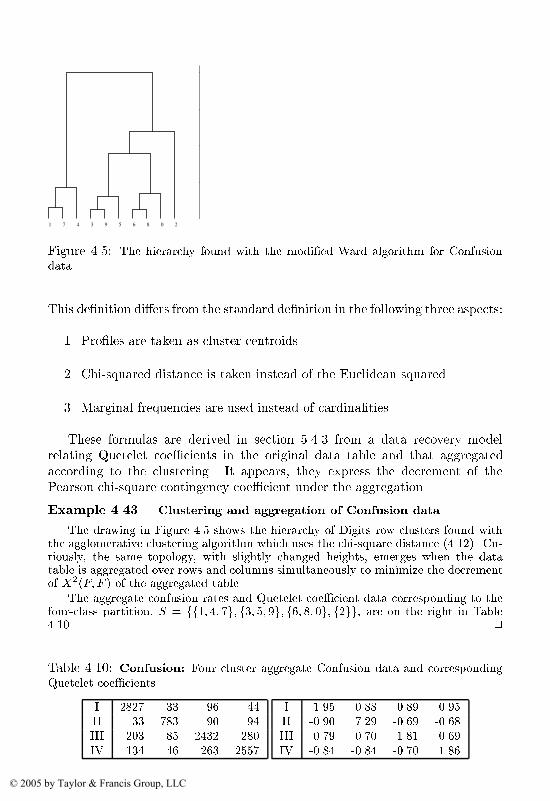
��� WARD HIERARCHICAL CLUSTERING
1 8 0 27 4 3 9 5 6
Figure ���� The hierarchy found with the modi�ed Ward algorithm for Confusiondata�
This denition di ers from the standard denition in the following three aspects�
�� Proles are taken as cluster centroids�
�� Chisquared distance is taken instead of the Euclidean squared�
�� Marginal frequencies are used instead of cardinalities�
These formulas are derived in section ����� from a data recovery modelrelating Quetelet coe�cients in the original data table and that aggregatedaccording to the clustering� It appears� they express the decrement of thePearson chisquare contingency coe�cient under the aggregation�
Example ����� Clustering and aggregation of Confusion data
The drawing in Figure ��� shows the hierarchy of Digits row clusters found withthe agglomerative clustering algorithm which uses the chi�square distance ����� � Cu�riously the same topology with slightly changed heights emerges when the datatable is aggregated over rows and columns simultaneously to minimize the decrementof X��F� F of the aggregated table�
The aggregate confusion rates and Quetelet coe�cient data corresponding to thefour�class partition S � ff�� �� �g� f�� �� �g� f�� �� g� f�gg are on the right in Table���� �
Table ����� Confusion� Four cluster aggregate Confusion data and correspondingQuetelet coe�cients�
I ���� �� �� ��II �� ��� � ��III �� �� ���� ��IV ��� �� ��� ����
I ���� ���� ���� ����II ��� ���� ���� ����III ���� ��� ���� ����IV ���� ���� ��� ����
© 2005 by Taylor & Francis Group, LLC
���� OVERALL ASSESSMENT ���
��� Overall assessment
Advantages of hierarchical clustering�
�� Visualizes the structure of similarities in a convenient form�
�� Models taxonomic classications�
�� Provides a bunch of interpretation aids at the level of entities� variables and variable covariances�
Less attractive features of the approach�
�� Massive computations related to nding minimum distances at eachstep� which is especially time consuming in agglomerative algorithms�
�� Rigidity� Having a splitting or merging step� no possibility to changeit afterwards�
Computations in agglomerative clustering can be drastically reduced if theminima from previous computations are kept�
© 2005 by Taylor & Francis Group, LLC
Chapter �
Data Recovery Models
Main subjects covered�
�� What is the data recovery approach�
�� A data recovery model and method for Principal component analysis�
�� A data recovery model and data scatter decomposition for KMeansand Anomalous cluster clustering�
�� A data recovery model and data scatter decompositions for clusterhierarchies�
�� A unied matrix equation model for all three above�
�� Mathematical properties of the models justifying methods presentedin previous chapters�
�� Extensions of the models� criteria and methods to similarity and contingency data�
�� Onebyone data recovery clustering methods�
�� Data recovery interpretation of correlation and association coe�cients�
Base words
Alternating optimization A method in the theory of optimization� applicable when a function to be optimized depends on two or more groups of
���
© 2005 by Taylor & Francis Group, LLC
��� DATA RECOVERY MODELS
variables� The method works iteratively by optimizing the function over agroup of variables having the other group specied� KMeans is a methodof alternating minimization of the square error clustering criterion�
Anomalous cluster A cluster which is furthest from the reference point�The iterated Anomalous clustering implements the onebyone separating strategy of Principal Component Analysis in the data recovery modelfor KMeans� and thus allows for extending KMeans to its intelligentversion� iKMeans� mitigating the need in dening an initial setting�
Attraction coe�cient A measure of attraction of an entity to a cluster�which is equal to the entity�s average similarity to the cluster minus halfof the average within cluster similarity� In KMeans and Ward clustering�attractions of entities to their clusters are greater than to other clusters�Moreover� in KMeans� entities are always positively attracted to theirclusters and negatively to other clusters�
Contingency data A data table whose rows and columns correspond to twosets of categories and entries are counts or proportions of observationsat the intersection of a row and column categories �cooccurrence values�� Because of their summability across the table� contingency data aretreated after having been transformed into relative Quetelet coe�cients�The data scatter of the transformed data is measured by the chisquarecontingency coe�cient�
Correspondence factor analysis A PCAlike method for visualization of cooccurrence values in a contingency table by displaying both row and column items as points in the same �D or �D space� Correspondence factoranalysis is a data recovery method in which the recovered entries areQuetelet association coe�cients� The method heavily relies on the singular value decomposition of a related matrix�
Data recovery models in clustering A data recovery model includes a rulewhich gives a value� according to a cluster structure� to every data entry�This way� every datum is represented as the sum of a clusterrecoveredvalue and a residual� which provides for a builtin quality principle� thesmaller the residuals� the better the cluster structure�
Data scatter decomposition A decomposition of the data scatter in twoparts� that explained by the cluster structure and that remaining unexplained� Such a decomposition provides for both an explicit clustercriterion and interpretation aids� the former being the minimum of theunexplained part and the latter various parts of the explained part� Theexplained part in KMeans and Ward clustering is always the sum ofcontributions of individual clusters or splits�
© 2005 by Taylor & Francis Group, LLC
BASE WORDS ���
Linear regression A method for analysis of interrelation between two quantitative features x and y in which y is approximated by an a�ne transformation ax! b of x� where a and b are referred to as slope and intercept�respectively� This setting is the genuine ground on which the coe�cientsof correlation and determination are dened and substantiated�
One�by�one clustering A method in clustering in which clusters or splits aretaken one by one� In this text� all such methods exploit the additivestructure of clustering data recovery models� which is analogous to thatof the model of Principal Component Analysis� Cluster separations andsplits are to be made in the order of their contribution to the data scatter�In this way� the additive structure of the data scatter decomposition ismaintained to provide for modelbased interpretation aids�
Principal component analysis A method for approximation of a data matrix with a small number of hidden factors� referred to as principal components� such that data entries are expressed as linear combinations ofhidden factor scores� It appears that principal components can be determined with the singular value decomposition �SVD� of the data matrix�
Reference point A vector in the variable space serving as the space origin�The Anomalous pattern is sought starting from an entity furthest from thereference point� which thus models the norm from which the Anomalouspattern deviates most�
Split versus separation Di erence between two perspectives� clusterversustherest and clusterversusthewhole� re�ected in di erent coe�cients attached to the distance between centroids of split parts� The former perspective is taken into account in the Wardlike divisive clustering methods�the latter in the Anomalous pattern clustering�
Ward�like divisive clustering A divisive clustering method using Ward distance as the splitting criterion� The method can be considered an implementation of the onebyone PCA strategy within the data recoveryclustering�
© 2005 by Taylor & Francis Group, LLC

��� DATA RECOVERY MODELS
��� Statistics modeling as data recovery
The data recovery approach is the cornerstone of contemporary thinking instatistics and data analysis� It is based on the assumption that the observeddata re�ect a regular structure in the phenomenon of which they inform� Theregular structure A� if known� would produce data F�A� that should coincidewith the observed data Y up to small residuals which are due to possible �awsin any or all of the following three aspects� �a� sampling entities� �b� selectingfeatures and tools for their measurements� and �c� modeling the phenomenon inquestion� Each of these can drastically a ect results� However� so far only thesimplest of the aspects� �a�� has been addressed scientically by introduction ofprobabilities to study the signicance of statistical inference in data analysis�In this treatise we are not concerned with these issues� We are concerned withthe underlying equation�
Observed data Y � Recovered data F�A� � Residuals E ��The quality of the model A is assessed according to the level of residuals
E� the smaller the residuals the better the model� Since quantitative modelsinvolve unknown coe�cients and parameters� this naturally leads to the ideaof tting these parameters to data in such a way that the residuals become assmall as possible� To put this idea as a minimization problem� one needs tocombine the multiple residuals in an aggregate criterion� In particular� the socalled principle of maximum likelihood has been developed in statistics� Whenthe data can be modelled as a random sample from a multivariate Gaussian distribution� this principle leads to the socalled least squares criterion� the sum ofsquared residuals to be minimized� In the data mining framework� the data donot necessarily come from a probabilistic population� Moreover� analysis of themechanism of data generation is not of primary concern� One needs only to seeif there are any patterns in the data as they are� In this case� the principle ofmaximum likelihood may be not applicable� Still� the sum of squared residualscriterion can be used in the context of data mining as a clear cut measure of thelargeness of the residuals� It provides for nice geometric properties and guaranties the production of provably reasonable cluster solutions� It admits usefuldecompositions of the data scatter into the sum of explained and unexplainedparts� No assumptions of particular distributions for the residuals are exploitedin the further treatment� To show the working of model �� along with the leastsquares principle� let us introduce four examples covering important methodsin data mining� �a� averaging� �b� linear regression� �c� principal componentanalysis� and �d� correspondence analysis� These examples are also used tointroduce some useful concepts in data analysis that are used throughout thistext�
© 2005 by Taylor & Francis Group, LLC
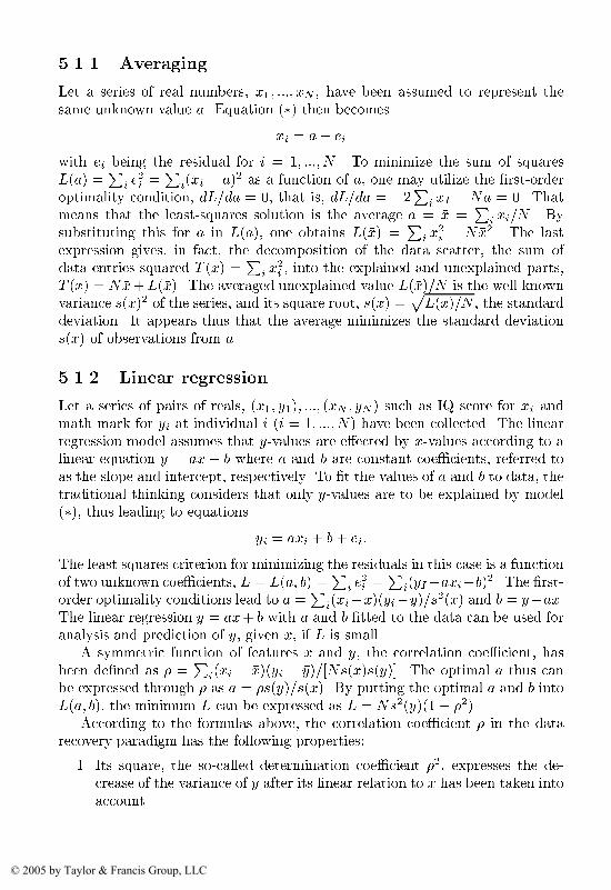
���� STATISTICS MODELING AS DATA RECOVERY ���
����� Averaging
Let a series of real numbers� x�� ���� xN � have been assumed to represent thesame unknown value a� Equation �� then becomes
xi � a! ei
with ei being the residual for i � �� ���� N � To minimize the sum of squaresL�a� �
Pi e
�i �
Pi�xi � a�� as a function of a� one may utilize the rstorder
optimality condition� dL�da � �� that is� dL�da � ��Pi xI �Na � �� Thatmeans that the leastsquares solution is the average a � "x �
Pi xi�N � By
substituting this for a in L�a�� one obtains L�"x� �P
i x�i � N "x�� The last
expression gives� in fact� the decomposition of the data scatter� the sum ofdata entries squared T �x� �
Pi x
�i � into the explained and unexplained parts�
T �x� � N "x!L�"x�� The averaged unexplained value L�"x��N is the well knownvariance s�x�� of the series� and its square root� s�x� �
pL�"x��N � the standard
deviation� It appears thus that the average minimizes the standard deviations�x� of observations from a�
����� Linear regression
Let a series of pairs of reals� �x�� y��� ���� �xN � yN � such as IQ score for xi andmath mark for yi at individual i �i � �� ���� N� have been collected� The linearregression model assumes that yvalues are e ected by xvalues according to alinear equation y � ax ! b where a and b are constant coe�cients� referred toas the slope and intercept� respectively� To t the values of a and b to data� thetraditional thinking considers that only yvalues are to be explained by model��� thus leading to equations
yi � axi ! b! ei�
The least squares criterion for minimizing the residuals in this case is a functionof two unknown coe�cients� L � L�a� b� �
Pi e
�i �
Pi�yI�axi�b��� The rst
order optimality conditions lead to a �P
i�xi� "x��yi� "y��s��x� and b � "y�a"x�The linear regression y � ax! b with a and b tted to the data can be used foranalysis and prediction of y� given x� if L is small�A symmetric function of features x and y� the correlation coe�cient� has
been dened as � �P
i�xi � "x��yi � "y���Ns�x�s�y��� The optimal a thus canbe expressed through � as a � �s�y��s�x�� By putting the optimal a and b intoL�a� b�� the minimum L can be expressed as L � Ns��y���� ����According to the formulas above� the correlation coe�cient � in the data
recovery paradigm has the following properties�
�� Its square� the socalled determination coe�cient ��� expresses the decrease of the variance of y after its linear relation to x has been taken intoaccount�
© 2005 by Taylor & Francis Group, LLC
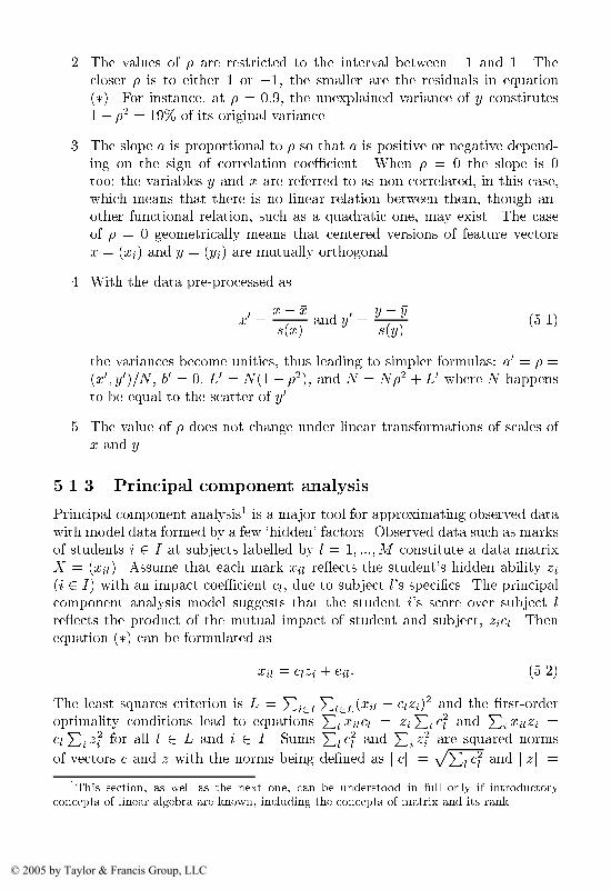
��� DATA RECOVERY MODELS
�� The values of � are restricted to the interval between �� and �� Thecloser � is to either � or ��� the smaller are the residuals in equation��� For instance� at � � ���� the unexplained variance of y constitutes�� �� � �� of its original variance�
�� The slope a is proportional to � so that a is positive or negative depending on the sign of correlation coe�cient� When � � � the slope is �too� the variables y and x are referred to as noncorrelated� in this case�which means that there is no linear relation between them� though another functional relation� such as a quadratic one� may exist� The caseof � � � geometrically means that centered versions of feature vectorsx � �xi� and y � �yi� are mutually orthogonal�
�� With the data preprocessed as
x� �x� "xs�x�
and y� �y � "ys�y�
�����
the variances become unities� thus leading to simpler formulas� a� � � ��x�� y���N � b� � �� L� � N��� ���� and N � N�� ! L� where N happensto be equal to the scatter of y��
�� The value of � does not change under linear transformations of scales ofx and y�
����� Principal component analysis
Principal component analysis� is a major tool for approximating observed datawith model data formed by a few �hidden� factors� Observed data such as marksof students i � I at subjects labelled by l � �� ����M constitute a data matrixX � �xil�� Assume that each mark xil re�ects the student�s hidden ability zi�i � I� with an impact coe�cient cl� due to subject l�s specics� The principalcomponent analysis model suggests that the student i�s score over subject lre�ects the product of the mutual impact of student and subject� zicl� Thenequation �� can be formulated as
xil � clzi ! eil� �����
The least squares criterion is L �P
i�I
Pl�L�xil � clzi�
� and the rstorderoptimality conditions lead to equations
Pl xilcl � zi
Pl c
�l and
Pi xilzi �
clP
i z�i for all l � L and i � I � Sums
Pl c
�l and
Pi z
�i are squared norms
of vectors c and z with the norms being dened as jjcjj � pPl c�l and jjzjj �
�This section� as well as the next one� can be understood in full only if introductoryconcepts of linear algebra are known� including the concepts of matrix and its rank�
© 2005 by Taylor & Francis Group, LLC
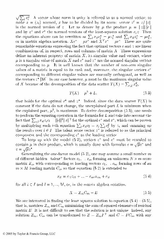
���� STATISTICS MODELING AS DATA RECOVERY ���
pPi z
�i � A vector whose norm is unity is referred to as a normed vector� to
make z � �zi� normed� z has to be divided by its norm� vector z� � z�jjzjj
is the normed version of z� Let us denote by � the product � � jjzjjjjcjjand by z� and c� the normed versions of the leastsquares solution c� z� Thenthe equations above can be rewritten as
Pl xilc
�l � �z�i and
Pi xilz
�i � �c�l �
or in matrix algebra notation� Xc� � �z� and XT z� � �c�� These are quiteremarkable equations expressing the fact that optimal vectors c and z are linearcombinations of� in respect� rows and columns of matrix X � These expressionsdene an inherent property of matrix X � its singular value and vectors� where� is a singular value of matrix X and c� and z� are the normed singular vectorscorresponding to �� It is well known that the number of nonzero singularvalues of a matrix is equal to its rank and� moreover� the singular vectors c�
corresponding to di erent singular values are mutually orthogonal� as well asthe vectors z� ����� In our case however� � must be the maximum singular valueof X because of the decomposition of the data scatter T �X� �
Pi�l x
�il�
T �X� � �� ! L� �����
that holds for the optimal c� and z�� Indeed� since the data scatter T �X� isconstant if the data do not change� the unexplained part L is minimum whenthe explained part� ��� is maximum� To derive decomposition ������ one needsto perform the squaring operation in the formula for L and take into account thefact that
Pi�l xilzicl � jjcjj�jjzjj� for the optimal c� and z�� which can be proven
by multiplying each ith equationP
l xilcl � ziP
l c�l by zi and summing up
the results over i � I � The talent score vector z� is referred to as the principalcomponent and the corresponding c� as the loading vector�To keep up with the model ������ vectors z� and c� must be rescaled to
contain � in their product� which is usually done with formulas c �p�c� and
z �p�z��
Generalizing the onefactor model ������ one may assume a small number mof di erent hidden �talent� factors z������ zm forming an unknown N m scorematrix Zm with corresponding m loading vectors c������ cm forming rows of anmM loading matrix Cm so that equation ����� is extended to
xil � c�lzi� ! ���! cmlzim ! eil �����
for all i � I and l � �� ����M � or� in the matrix algebra notation�
X � ZmCm !E �����
We are interested in nding the least squares solution to equation ����� � ������that is� matrices Zm and Cm minimizing the sum of squared elements of residualmatrix E� It is not di�cult to see that the solution is not unique� Indeed� anysolution Zm� Cm can be transformed to Z � ZmF
T and C � FCm with any
© 2005 by Taylor & Francis Group, LLC
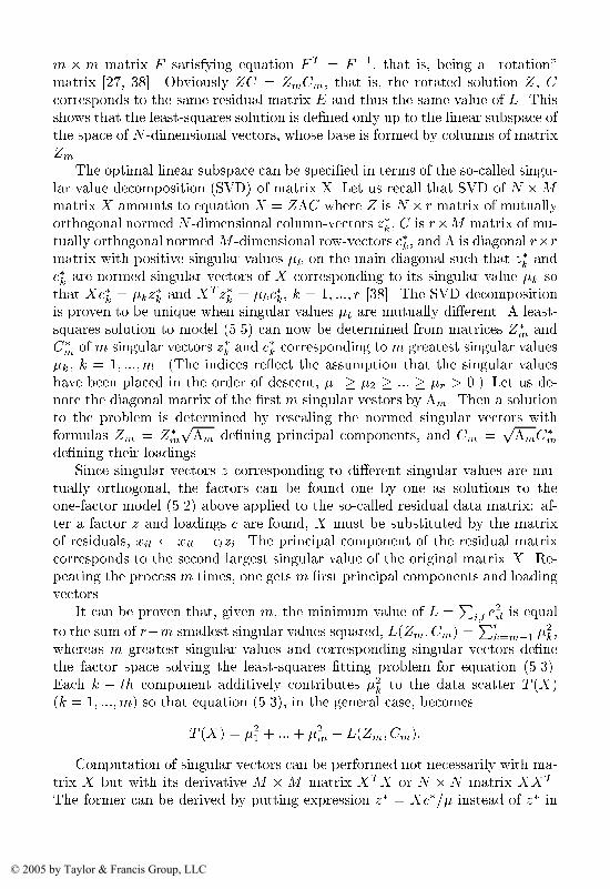
��� DATA RECOVERY MODELS
m m matrix F satisfying equation F T � F��� that is� being a �rotation�matrix ���� ���� Obviously ZC � ZmCm� that is� the rotated solution Z� Ccorresponds to the same residual matrix E and thus the same value of L� Thisshows that the leastsquares solution is dened only up to the linear subspace ofthe space of N dimensional vectors� whose base is formed by columns of matrixZm�The optimal linear subspace can be specied in terms of the socalled singu
lar value decomposition �SVD� of matrix X� Let us recall that SVD of N Mmatrix X amounts to equation X � Z&C where Z is N r matrix of mutuallyorthogonal normed N dimensional columnvectors z�k � C is rM matrix of mutually orthogonal normedM dimensional rowvectors c�k� and & is diagonal rrmatrix with positive singular values �k on the main diagonal such that z
�k and
c�k are normed singular vectors of X corresponding to its singular value �k sothat Xc�k � �kz
�k and X
T z�k � �kc�k� k � �� ���� r ����� The SVD decomposition
is proven to be unique when singular values �t are mutually di erent� A leastsquares solution to model ����� can now be determined from matrices Z�
m andC�m of m singular vectors z
�k and c
�k corresponding to m greatest singular values
�k� k � �� ����m� �The indices re�ect the assumption that the singular valueshave been placed in the order of descent� �� � �� � ��� � �r � ��� Let us denote the diagonal matrix of the rst m singular vestors by &m� Then a solutionto the problem is determined by rescaling the normed singular vectors withformulas Zm � Z�
m
p&m dening principal components� and Cm �
p&mC
�m
dening their loadings�Since singular vectors z corresponding to di erent singular values are mu
tually orthogonal� the factors can be found one by one as solutions to theonefactor model ����� above applied to the socalled residual data matrix� after a factor z and loadings c are found� X must be substituted by the matrixof residuals� xil � xil � clzi� The principal component of the residual matrixcorresponds to the second largest singular value of the original matrix X � Repeating the process m times� one gets m rst principal components and loadingvectors�It can be proven that� given m� the minimum value of L �
Pi�l e
�il is equal
to the sum of r�m smallest singular values squared� L�Zm� Cm� �Pr
k�m�� ��k�
whereas m greatest singular values and corresponding singular vectors denethe factor space solving the leastsquares tting problem for equation ������Each k � th component additively contributes ��k to the data scatter T �X��k � �� ����m� so that equation ������ in the general case� becomes
T �X� � ��� ! ���! ��m ! L�Zm� Cm��
Computation of singular vectors can be performed not necessarily with matrix X but with its derivative M M matrix XTX or N N matrix XXT �The former can be derived by putting expression z� � Xc��� instead of z� in
© 2005 by Taylor & Francis Group, LLC
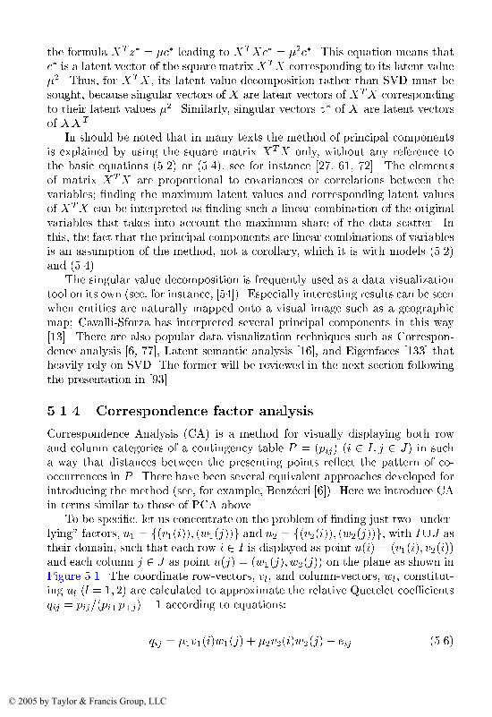
���� STATISTICS MODELING AS DATA RECOVERY ���
the formula XT z� � �c� leading to XTXc� � ��c�� This equation means thatc� is a latent vector of the square matrix XTX corresponding to its latent value��� Thus� for XTX � its latent value decomposition rather than SVD must besought� because singular vectors of X are latent vectors of XTX correspondingto their latent values ��� Similarly� singular vectors z� of X are latent vectorsof XXT �In should be noted that in many texts the method of principal components
is explained by using the square matrix XTX only� without any reference tothe basic equations ����� or ������ see for instance ���� ��� ���� The elementsof matrix XTX are proportional to covariances or correlations between thevariables� nding the maximum latent values and corresponding latent valuesof XTX can be interpreted as nding such a linear combination of the originalvariables that takes into account the maximum share of the data scatter� Inthis� the fact that the principal components are linear combinations of variablesis an assumption of the method� not a corollary� which it is with models �����and ������The singular value decomposition is frequently used as a data visualization
tool on its own �see� for instance� ������ Especially interesting results can be seenwhen entities are naturally mapped onto a visual image such as a geographicmap� CavalliSforza has interpreted several principal components in this way����� There are also popular data visualization techniques such as Correspondence analysis ��� ���� Latent semantic analysis ����� and Eigenfaces ����� thatheavily rely on SVD� The former will be reviewed in the next section followingthe presentation in �����
����� Correspondence factor analysis
Correspondence Analysis �CA� is a method for visually displaying both rowand column categories of a contingency table P � �pij� �i � I� j � J� in sucha way that distances between the presenting points re�ect the pattern of cooccurrences in P � There have been several equivalent approaches developed forintroducing the method �see� for example� Benz�ecri ����� Here we introduce CAin terms similar to those of PCA above�To be specic� let us concentrate on the problem of nding just two �under
lying� factors� u� � f�v��i��� �w��j��g and u� � f�v��i��� �w��j��g� with I �J astheir domain� such that each row i � I is displayed as point u�i� � �v��i�� v��i��and each column j � J as point u�j� � �w��j�� w��j�� on the plane as shown inFigure ���� The coordinate rowvectors� vl� and columnvectors� wl� constituting ul �l � �� �� are calculated to approximate the relative Quetelet coe�cientsqij � pij��pi�p�j�� � according to equations�
qij � ��v��i�w��j� ! ��v��i�w��j� ! eij �����
© 2005 by Taylor & Francis Group, LLC
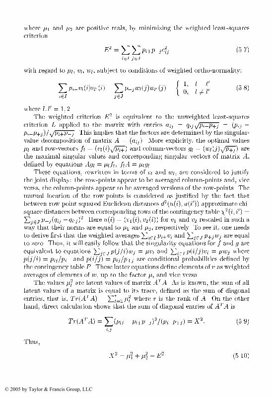
��� DATA RECOVERY MODELS
where �� and �� are positive reals� by minimizing the weighted leastsquarescriterion
E� �Xi�I
Xj�J
pi�p�je�ij �����
with regard to �l� vl� wl� subject to conditions of weighted orthonormality�
Xi�I
pi�vl�i�vl��i� �Xj�J
p�jwl�j�wl� �j� �
��� l � l�
�� l � l������
where l� l� � �� ��The weighted criterion E� is equivalent to the unweighted leastsquares
criterion L applied to the matrix with entries aij � qijppi�p�j � �pij �
pi�p�j��ppi�p�j � This implies that the factors are determined by the singular
value decomposition of matrix A � �aij�� More explicitly� the optimal values�l and rowvectors fl � �vl�i�
ppi�� and columnvectors gl � �wl�j�
pp�j� are
the maximal singular values and corresponding singular vectors of matrix A�dened by equations Agl � �lfl� flA � �lgl�These equations� rewritten in terms of vl and wl� are considered to justify
the joint display� the rowpoints appear to be averaged columnpoints and� viceversa� the columnpoints appear to be averaged versions of the rowpoints� Themutual location of the rowpoints is considered as justied by the fact thatbetweenrowpoint squared Euclidean distances d��u�i�� u�i��� approximate chisquare distances between corresponding rows of the contingency table ���i� i�� �P
j�J p�j�qij � qi�j��� Here u�i� � �v��i�� v��i�� for v� and v� rescaled in such a
way that their norms are equal to �� and ��� respectively� To see it� one needsto derive rst that the weighted averages
Pi�I pi�vi and
Pj�J p�jwj are equal
to zero� Then� it will easily follow that the singularity equations for f and g areequivalent to equations
Pj�J p�j�i�wj � �vi and
Pi�I p�i�j�vi � �wj where
p�j�i� � pij�pi� and p�i�j� � pij�p�j are conditional probabilities dened bythe contingency table P � These latter equations dene elements of v as weightedaverages of elements of w� up to the factor �� and vice versa�The values ��l are latent values of matrix A
TA� As is known� the sum of alllatent values of a matrix is equal to its trace� dened as the sum of diagonalentries� that is� Tr�ATA� �
Prt�� �
�t where r is the rank of A� On the other
hand� direct calculation shows that the sum of diagonal entries of ATA is
Tr�ATA� �Xi�j
�pij � pi�p�j����pi�p�j� � X�� �����
Thus�
X� � ��� ! ��� !E� ������
© 2005 by Taylor & Francis Group, LLC
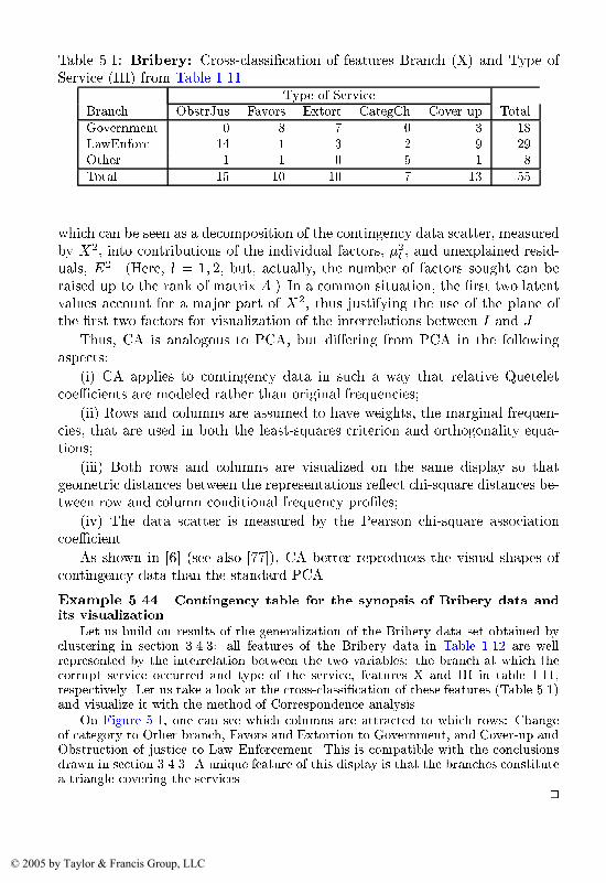
���� STATISTICS MODELING AS DATA RECOVERY ���
Table ���� Bribery� Crossclassication of features Branch �X� and Type ofService �III� from Table �����
Type of ServiceBranch ObstrJus Favors Extort CategCh Cover�up Total
Government � � � ��LawEnforc �� � � � � ��Other � � � � �
Total �� � � � �� ��
which can be seen as a decomposition of the contingency data scatter� measuredby X�� into contributions of the individual factors� ��l � and unexplained residuals� E�� �Here� l � �� �� but� actually� the number of factors sought can beraised up to the rank of matrix A�� In a common situation� the rst two latentvalues account for a major part of X�� thus justifying the use of the plane ofthe rst two factors for visualization of the interrelations between I and J �
Thus� CA is analogous to PCA� but di ering from PCA in the followingaspects�
�i� CA applies to contingency data in such a way that relative Queteletcoe�cients are modeled rather than original frequencies�
�ii� Rows and columns are assumed to have weights� the marginal frequencies� that are used in both the leastsquares criterion and orthogonality equations�
�iii� Both rows and columns are visualized on the same display so thatgeometric distances between the representations re�ect chisquare distances between row and column conditional frequency proles�
�iv� The data scatter is measured by the Pearson chisquare associationcoe�cient�
As shown in ��� �see also ������ CA better reproduces the visual shapes ofcontingency data than the standard PCA�
Example ����� Contingency table for the synopsis of Bribery data andits visualization
Let us build on results of the generalization of the Bribery data set obtained byclustering in section ������ all features of the Bribery data in Table ���� are wellrepresented by the interrelation between the two variables� the branch at which thecorrupt service occurred and type of the service features X and III in table ����respectively� Let us take a look at the cross�classi�cation of these features �Table ��� and visualize it with the method of Correspondence analysis�
On Figure ��� one can see which columns are attracted to which rows� Changeof category to Other branch Favors and Extortion to Government and Cover�up andObstruction of justice to Law Enforcement� This is compatible with the conclusionsdrawn in section ������ A unique feature of this display is that the branches constitutea triangle covering the services�
�
© 2005 by Taylor & Francis Group, LLC
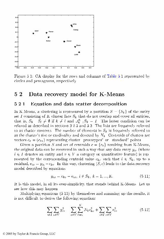
��� DATA RECOVERY MODELS
−0.6 −0.5 −0.4 −0.3 −0.2 −0.1 0 0.1 0.2 0.3 0.4−0.6
−0.5
−0.4
−0.3
−0.2
−0.1
0
0.1
0.2
0.3
0.4
GOV
LAW
OTH
Obstr
Favor
Extor
Categ
Cover
Figure ���� CA display for the rows and columns of Table ��� represented bycircles and pentagrams� respectively�
��� Data recovery model for K�Means
����� Equation and data scatter decomposition
In KMeans� a clustering is represented by a partition S � fSkg of the entityset I consisting of K cluster lists Sk that do not overlap and cover all entities�that is� Sk � Sl � � if k � l and �Kk��Sk � I � The latter condition can berelaxed as described in sections ����� and ���� The lists are frequently referredto as cluster contents� The number of elements in Sk is frequently referred toas the cluster�s size or cardinality and denoted by Nk� Centroids of clusters arevectors ck � �ckv� representing cluster �prototypes� or �standard� points�Given a partition S and set of centroids c � fckg resulting from KMeans�
the original data can be recovered in such a way that any data entry yiv �wherei � I denotes an entity and v � V a category or quantitative feature� is represented by the corresponding centroid value ckv such that i � Sk� up to aresidual� eiv � yiv�ckv � In this way� clustering �S� c� leads to the data recoverymodel described by equations
yiv � ckv ! eiv � i � Sk� k � �� ����K� ������
It is this model� in all its oversimplicity� that stands behind KMeans� Let ussee how this may happen�Multiplying equations ������ by themselves and summing up the results� it
is not di�cult to derive the following equation�
Xi�I
Xv�V
y�iv �Xv�V
KXk��
Nkc�kv !
Xi�I
Xv�V
e�iv ������
© 2005 by Taylor & Francis Group, LLC
���� DATA RECOVERY MODEL FOR K�MEANS ���
The derivation is based on the assumption that ckv is the average of withincluster values yiv � i � Sk� so that
Pi�Sk
ckvyiv � Nkc�kv � Noting that the
righthand term in �������P
i�I
Pv�V e�iv �
PMk��
Pi�Sk
Pv�V �yiv � ckv�
� �PMk��
Pi�Sk
d�yi� ck�� is KMeans square error criterionW �S� c� ������ equation������ can be rewritten as
T �Y � � B�S� c� !W �S� c� ������
where T �Y � �P
i�v y�iv is the data scatter� W �S� c� �
PMk��
Pi�Sk
d�yi� ck�squareerror clustering criterion and B�S� c� the middle term in decomposition�������
B�S� c� �Xv�V
KXk��
c�kvNk ������
Equation ������� or its equivalent ������� is wellknown in the analysis of variance� its parts B�S� c� and W �S� c� are conventionally referred to as betweengroup and withingroup variance in statistics� In the context of model ������these� however� denote the explained and unexplained parts of the data scatter�respectively� The square error criterion of KMeans� therefore� minimizes theunexplained part of the data scatter� or� equivalently� maximizes the explainedpart� B�S� c� ������� In other words� this criterion expresses the idea of approximation of data Y by the KMeans partitioning as expressed in equation�������Equation ������ can be rewritten in terms of distances d since
T�Y��PN
i�� d�yi� �� and B�S� c� �PK
k��Nkd�ck� �� according to the denitionof the Euclidean distance squared�
NXi��
d�yi� �� �
KXk��
Nkd�ck � �� !
KXk��
NXi��
d�yi� ck� ������
����� Contributions of clusters� features� and individualentities
According to equations ������ and ������� each individual cluster k � �� ���Kadditively contributes
B�Sk� ck� �Xv�V
c�kvNk ������
to B�S� c�� In its turn� any individual cluster�s contribution is the sum of clusterspecic feature contributions Bvk � c�kvNk� Following from the preliminary
© 2005 by Taylor & Francis Group, LLC
��� DATA RECOVERY MODELS
standardization of data by subtracting features� grand means� the contributionBvk is proportional to the squared di erence between variable v�s grand meancv and its within cluster mean ckv � the larger the di erence the greater thecontribution� This nicely ts into our intuition� the farther away is the clusterfrom the grand mean on a feature range� the more useful should be the featurein separating the cluster from the rest�To evaluate contributions of individual entities to the explained part of
the data scatter� one needs yet another reformulation of ������� Let us referto the denition ckv �
Pi�Sk
yiv�Nk and put it into c�kvNk �halfway�� This
then becomes c�kvNk �P
i�Skyivckv leading to B�Sk� ck� reformulated as the
summary inner product�
B�Sk� ck� �Xv�V
Xi�Sk
yivckv �Xi�Sk
�yi� ck�� ������
thus suggesting that the contribution of entity i � Sk to the explained part ofthe data scatter is �yi� ck�� the inner product between the entity point and thecluster�s centroid� as follows from ������ This may give further insights into thescatter decomposition to highlight contributions of individual entities �see anexample in Table ������These and related interpretation aids are suggested for use in section �����
as a nonconventional but informative instrument�
����� Correlation ratio as contribution
To measure statistical association between a quantitative feature v and partitionS � fS�� ���� SKg� the socalled correlation ratio � has been dened in statistics�
��S� v� � �v �
PKk�� pk
�kv
�v������
where �v �P
i�I �xiv � cv���N and �kv �
Pi�Sk
�xiv � ckv���Nk are the vari
ance and withincluster variance of variable v� respectively� before data preprocessing and pk � Nk�N � Actually� the correlation ratio expresses the extentto which the withincluster averages can be used as predicted values of v and� inthis sense� is analogous to the determination coe�cient in the model of linear regression� The correlation ratio ranges between � and �� and it is equal to � onlywhen all the withinclass variances are zero� The greater the withincategoryvariances� the smaller the correlation ratio�Assuming that the raw data xiv have been standardized to yiv � �xiv�cv��bv
by shifting the origins to cv and rescaling results by dividing them over bv� itis not di�cult to prove that the total contribution B�S� v� �
PKk�� Bvk �PK
k�� c�kvNk of a quantitative feature v to the clusterexplained part of the
data scatter in ������ equals to N��S� v� �v�b�v �����
© 2005 by Taylor & Francis Group, LLC
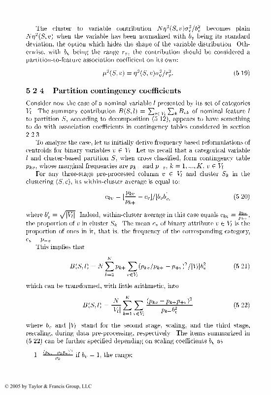
���� DATA RECOVERY MODEL FOR K�MEANS ���
The cluster to variable contribution N��S� v� �v�b�v becomes plain
N��S� v� when the variable has been normalized with bv being its standarddeviation� the option which hides the shape of the variable distribution� Otherwise� with bv being the range rv � the contribution should be considered apartitiontofeature association coe�cient on its own�
���S� v� � ��S� v� �v�r�v� ������
����� Partition contingency coe cients
Consider now the case of a nominal variable l presented by its set of categoriesVl� The summary contribution B�S� l� �
Pv�Vl
Pk Bvk of nominal feature l
to partition S� according to decomposition ������� appears to have somethingto do with association coe�cients in contingency tables considered in section������To analyze the case� let us initially derive frequency based reformulations of
centroids for binary variables v � Vl� Let us recall that a categorical variablel and clusterbased partition S� when cross classied� form contingency tablepkv � whose marginal frequencies are pk� and p�v� k � �� ����K� v � Vl�For any threestage preprocessed column v � Vl and cluster Sk in the
clustering �S� c�� its withincluster average is equal to�
ckv � �pkvpk�
� cv ���bvb�
v� ������
where b�v �pjVlj� Indeed� withincluster average in this case equals ckv � pkv
pk��
the proportion of v in cluster Sk� The mean cv of binary attribute v � Vl is theproportion of ones in it� that is� the frequency of the corresponding category�cv � p�v�This implies that
B�S� l� � N
KXk��
pk�Xv�Vl
�pkv�pk� � p�v���jVljb�v ������
which can be transformed� with little arithmetic� into
B�S� l� �N
jVljKXk��
Xv�Vl
�pkv � pk�p�v��
pk�b�v������
where bv and jVlj stand for the second stage� scaling� and the third stage�rescaling� during data preprocessing� respectively� The items summarized in������ can be further specied depending on scaling coe�cients bv as
�� �pkv�pkpv��
pkif bv � �� the range�
© 2005 by Taylor & Francis Group, LLC

��� DATA RECOVERY MODELS
�� �pkv�pkpv��
pkpv���pv�if bv �
ppv��� pv�� Bernoulli standard deviation�
�� �pkv�pkpv��
pkpvif bu �
ppu� Poisson standard deviation�
These lead to the following statement�
Statement ���� The contribution B�S� l� of a nominal variable l and partitionS to the explained part of the data scatter� depending on the standardizing co�e�cients� is equal to contingency coe�cient G� ��� or Q� � X��N ����if scaling coe�cients bv are taken to be bv � � or bv �
pp�v� respectively� and
rescaling coe�cients b�v � �� It is further divided by the number of categoriesjVlj if rescaling coe�cients are b�v �
pjVlj for v � Vl�
Two well known normalizations of the Pearson chisquare contingency coe�cient are due to Tchouprov� T � X��
p�K � ���jVlj � ��� and Cramer�
C � X��min�K � �� jVlj � ��� both symmetric over the numbers of categoriesand clusters� The statement ���� implies one more� asymmetric� normalizationof X�� M � X��jVlj� as a meaningful part of the data scatter in the clusteringproblem�When the chisquare contingency coe�cient or related indexes are applied
in the traditional statistics context� the presence of zeros in a contingency tablebecomes an issue because it contradicts the hypothesis of statistical independence� In the context of data recovery clustering� zeros are treated as any othernumbers and create no problems at all because the coe�cients are measures ofcontributions and bear no other statistical meaning in this context�
��� Data recovery models for Ward criterion
����� Data recovery models with cluster hierarchies
To formulate supporting models for agglomerative and divisive Ward clustering�one needs to explicitly dene the concepts of cluster tree and hierarchy� A setS of subsets Sw � I is called nested if for every two subsets Sw and Sw� fromS either one of them is part of the other or they do not overlap at all� Given anested set S� Sw � S is referred to as a child of Sw� � S if Sw � Sw� and no othersubset Sw�� � S exists such that Sw � Sw�� � Sw� � A subset Sw � S is referredto as a terminal node or leaf if Sw has no children in S� A nested set S will bereferred to as a cluster hierarchy over I if any nonterminal subset Sw � S hastwo children Sw� � Sw�� � S covering it entirely so that Sw� � Sw�� � Sw� Thesubsets Sw � S will be referred to as clusters�Two types of cluster hierarchy are of interest in modeling clustering al
gorithms� those S containing singleton clusters fig for all i � I and thosecontaining set I itself as a cluster� The former will be referred to as the lower
© 2005 by Taylor & Francis Group, LLC

���� DATA RECOVERY MODELS FOR WARD CRITERION ���
cluster hierarchy and the latter� the upper cluster hierarchy� A lower hierarchycan be thought of as resulting from an agglomerative clustering algorithm andan upper hierarchy from a divisive clustering algorithm� A complete result ofa clustering algorithm of either type can be represented by a cluster tree� thatis� a cluster hierarchy which is both lower and upper�For an upper cluster hierarchy S� let us denote the set of its leaves by L�S��
it is obviously a partition of I � Similarly� for a lower cluster hierarchy S� let usdenote its set of maximal clusters by M�S�� this is also a partition of I �Given an upper or lower cluster hierarchy S over set I and a preprocessed
data matrix Y � �yiv�� let us� for any feature v� denote the average value of yivwithin Sw � S by cwv�Given an upper cluster hierarchy S� let us consider its leaf partition L�S��
For any data entry yiv and a leaf cluster Sw� � L�S� containing it� the modelunderlying KMeans suggests that yiv is equal to cw�v up to the residual eiv �yiv � cw�v� Obviously� eiv � � if Sw� is a singleton consisting of just one entityi� To extend this to the hierarchy S� let us denote the set of all nonsingletonclusters containing i by Si and add to and subtract from the equation theaverages of feature v within each Sw � Si� This leads us to the followingequation�
yiv �X
Sw�Si
�cw��v � cwv� ! eiv ������
where Sw� is a child of Sw that runs through Si� Obviously� all eiv � � in ������if S is a cluster tree�
����� Covariances� variances and data scatter decomposed
Model in ������ is not just a trivial extension of the KMeans model to the caseof upper cluster hierarchies� in spite of the fact that the only �real� item in thesum in ������ is cw�v where Sw� is the leaf cluster containing i� Indeed� theequation implies the following decomposition�
Statement ���� For every feature columns v� u � V in the pre�processed datamatrix Y � their inner product can be decomposed over the cluster hierarchy Sas follows�
�yv � yu� �Xw
Nw�Nw�
Nw�cw��v � cw��v��cw��u � cw��u� ! �ev� eu� ������
where w runs over all nonterminal clusters Sw � S with children Sw� and Sw� Nw� Nw�� Nw� being their respective cardinalities�
Proof� The proof follows from equation Nwcw � Nw�cw� !Nw�cw� which relates the centroid of a nonterminal cluster Sw with those of its children� By
© 2005 by Taylor & Francis Group, LLC
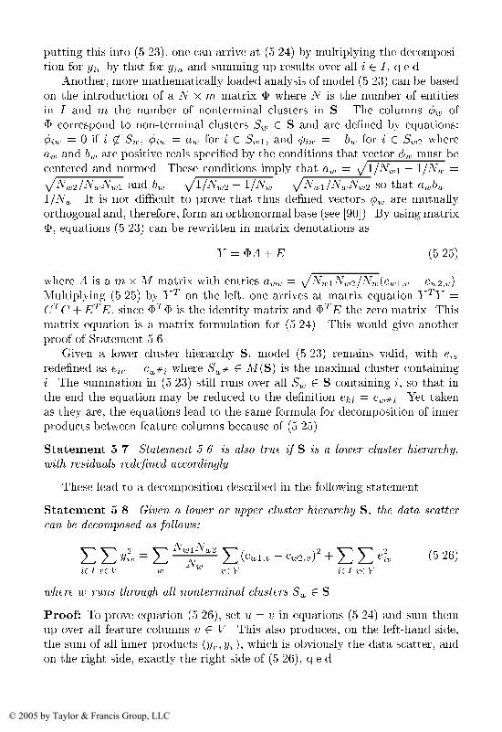
��� DATA RECOVERY MODELS
putting this into ������� one can arrive at ������ by multiplying the decomposition for yiv by that for yiu and summing up results over all i � I � q�e�d�Another� more mathematically loaded analysis of model ������ can be based
on the introduction of a N m matrix ' where N is the number of entitiesin I and m the number of nonterminal clusters in S� The columns �w of' correspond to nonterminal clusters Sw � S and are dened by equations��iw � � if i � Sw� �iw � aw for i � Sw�� and �iw � �bw for i � Sw� whereaw and bw are positive reals specied by the conditions that vector �w must becentered and normed� These conditions imply that aw �
p��Nw� � ��Nw �p
Nw��NwNw� and bw �p��Nw� � ��Nw �
pNw��NwNw� so that awbw �
��Nw� It is not di�cult to prove that thus dened vectors �w are mutuallyorthogonal and� therefore� form an orthonormal base �see ������ By using matrix'� equations ������ can be rewritten in matrix denotations as
Y � 'A!E ������
where A is a mM matrix with entries awv �pNw�Nw��Nw�cw��v � cw��v��
Multiplying ������ by Y T on the left� one arrives at matrix equation Y TY �CTC !ETE� since 'T' is the identity matrix and 'TE the zero matrix� Thismatrix equation is a matrix formulation for ������� This would give anotherproof of Statement ����Given a lower cluster hierarchy S� model ������ remains valid� with eiv
redened as eiv � cw�i where Sw� � M�S� is the maximal cluster containingi� The summation in ������ still runs over all Sw � S containing i� so that inthe end the equation may be reduced to the denition ehi � cw�i� Yet takenas they are� the equations lead to the same formula for decomposition of innerproducts between feature columns because of �������
Statement ���� Statement ���� is also true if S is a lower cluster hierarchy�with residuals rede�ned accordingly�
These lead to a decomposition described in the following statement�
Statement ���� Given a lower or upper cluster hierarchy S� the data scattercan be decomposed as follows�
Xi�I
Xv�V
y�iv �Xw
Nw�Nw�
Nw
Xv�V
�cw��v � cw��v�� !Xi�I
Xv�V
e�iv ������
where w runs through all nonterminal clusters Sw � S�Proof� To prove equation ������� set u � v in equations ������ and sum themup over all feature columns v � V � This also produces� on the lefthand side�the sum of all inner products �yv � yv�� which is obviously the data scatter� andon the right side� exactly the right side of ������� q�e�d�
© 2005 by Taylor & Francis Group, LLC
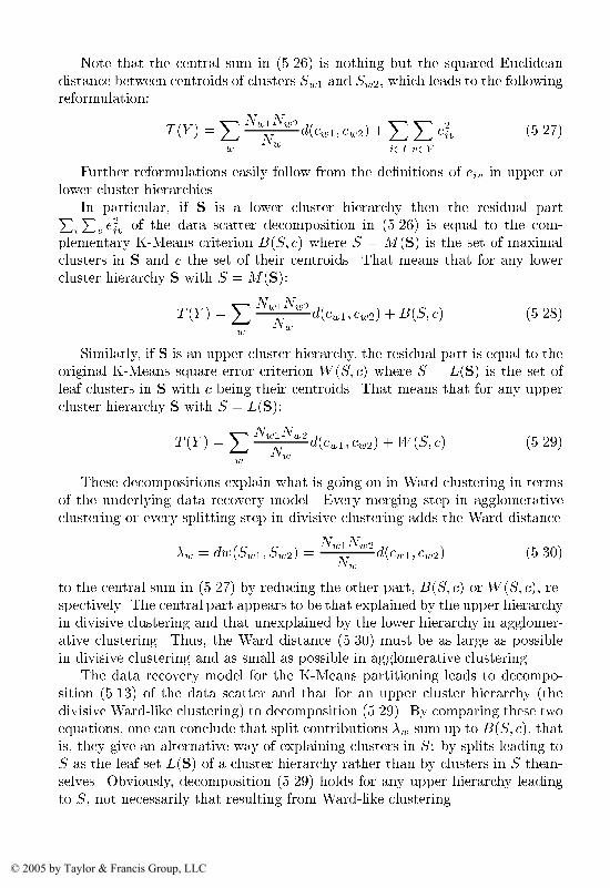
���� DATA RECOVERY MODELS FOR WARD CRITERION ���
Note that the central sum in ������ is nothing but the squared Euclideandistance between centroids of clusters Sw� and Sw�� which leads to the followingreformulation�
T �Y � �Xw
Nw�Nw�
Nwd�cw�� cw�� !
Xi�I
Xv�V
e�iv ������
Further reformulations easily follow from the denitions of eiv in upper orlower cluster hierarchies�In particular� if S is a lower cluster hierarchy then the residual partPi
Pv e
�iv of the data scatter decomposition in ������ is equal to the com
plementary KMeans criterion B�S� c� where S � M�S� is the set of maximalclusters in S and c the set of their centroids� That means that for any lowercluster hierarchy S with S �M�S��
T �Y � �Xw
Nw�Nw�
Nwd�cw�� cw�� !B�S� c� ������
Similarly� if S is an upper cluster hierarchy� the residual part is equal to theoriginal KMeans square error criterion W �S� c� where S � L�S� is the set ofleaf clusters in S with c being their centroids� That means that for any uppercluster hierarchy S with S � L�S��
T �Y � �Xw
Nw�Nw�
Nwd�cw�� cw�� !W �S� c� ������
These decompositions explain what is going on in Ward clustering in termsof the underlying data recovery model� Every merging step in agglomerativeclustering or every splitting step in divisive clustering adds the Ward distance
w � dw�Sw�� Sw�� �Nw�Nw�
Nwd�cw�� cw�� ������
to the central sum in ������ by reducing the other part� B�S� c� or W �S� c�� respectively� The central part appears to be that explained by the upper hierarchyin divisive clustering and that unexplained by the lower hierarchy in agglomerative clustering� Thus� the Ward distance ������ must be as large as possiblein divisive clustering and as small as possible in agglomerative clustering�The data recovery model for the KMeans partitioning leads to decompo
sition ������ of the data scatter and that for an upper cluster hierarchy �thedivisive Wardlike clustering� to decomposition ������� By comparing these twoequations� one can conclude that split contributions w sum up to B�S� c�� thatis� they give an alternative way of explaining clusters in S� by splits leading toS as the leaf set L�S� of a cluster hierarchy rather than by clusters in S themselves� Obviously� decomposition ������ holds for any upper hierarchy leadingto S� not necessarily that resulting from Wardlike clustering�
© 2005 by Taylor & Francis Group, LLC
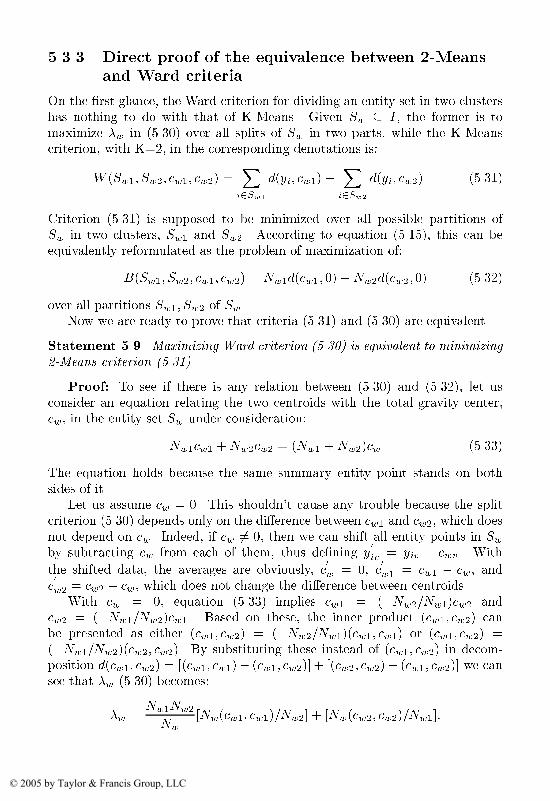
��� DATA RECOVERY MODELS
����� Direct proof of the equivalence between �Meansand Ward criteria
On the rst glance� the Ward criterion for dividing an entity set in two clustershas nothing to do with that of KMeans� Given Sw � I � the former is tomaximize w in ������ over all splits of Sw in two parts� while the KMeanscriterion� with K��� in the corresponding denotations is�
W �Sw�� Sw�� cw�� cw�� �Xi�Sw�
d�yi� cw�� !Xi�Sw�
d�yi� cw�� ������
Criterion ������ is supposed to be minimized over all possible partitions ofSw in two clusters� Sw� and Sw�� According to equation ������� this can beequivalently reformulated as the problem of maximization of�
B�Sw�� Sw�� cw�� cw�� � Nw�d�cw�� �� !Nw�d�cw�� �� ������
over all partitions Sw�� Sw� of Sw�Now we are ready to prove that criteria ������ and ������ are equivalent�
Statement ���� Maximizing Ward criterion ����� is equivalent to minimizing��Means criterion �����
Proof� To see if there is any relation between ������ and ������� let usconsider an equation relating the two centroids with the total gravity center�cw� in the entity set Sw under consideration�
Nw�cw� !Nw�cw� � �Nw� !Nw��cw ������
The equation holds because the same summary entity point stands on bothsides of it�Let us assume cw � �� This shouldn�t cause any trouble because the split
criterion ������ depends only on the di erence between cw� and cw�� which doesnot depend on cw� Indeed� if cw � �� then we can shift all entity points in Swby subtracting cw from each of them� thus dening y
�
iv � yiv � cwv� With
the shifted data� the averages are obviously� c�
w � �� c�
w� � cw� � cw� andc�
w� � cw� � cw� which does not change the di erence between centroids�With cw � �� equation ������ implies cw� � ��Nw��Nw��cw� and
cw� � ��Nw��Nw��cw�� Based on these� the inner product �cw�� cw�� canbe presented as either �cw�� cw�� � ��Nw��Nw���cw�� cw�� or �cw�� cw�� ���Nw��Nw���cw�� cw��� By substituting these instead of �cw�� cw�� in decomposition d�cw�� cw�� � ��cw�� cw��� �cw�� cw��� ! ��cw�� cw��� �cw�� cw��� we cansee that w ������ becomes�
w �Nw�Nw�
Nw�Nw�cw�� cw���Nw�� ! �Nw�cw�� cw���Nw���
© 2005 by Taylor & Francis Group, LLC
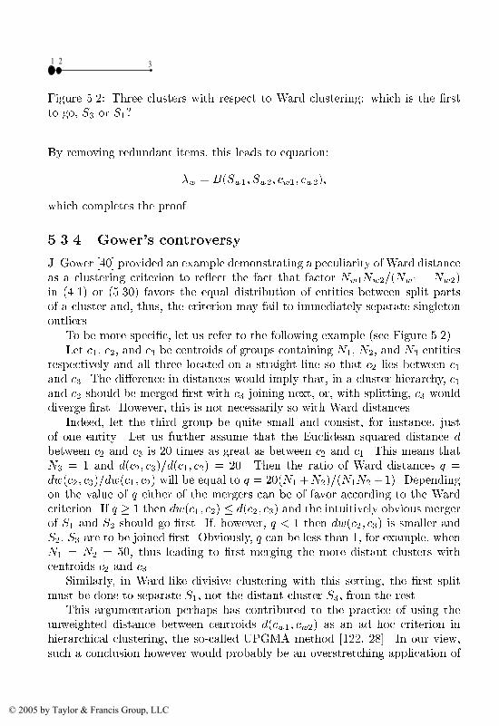
���� DATA RECOVERY MODELS FOR WARD CRITERION ���
2 3 1
Figure ���� Three clusters with respect to Ward clustering� which is the rstto go� S� or S��
By removing redundant items� this leads to equation�
w � B�Sw�� Sw�� cw�� cw���
which completes the proof�
����� Gower�s controversy
J� Gower ���� provided an example demonstrating a peculiarity of Ward distanceas a clustering criterion to re�ect the fact that factor Nw�Nw���Nw� ! Nw��in ����� or ������ favors the equal distribution of entities between split partsof a cluster and� thus� the criterion may fail to immediately separate singletonoutliers�To be more specic� let us refer to the following example �see Figure �����Let c�� c�� and c� be centroids of groups containing N�� N�� and N� entities
respectively and all three located on a straight line so that c� lies between c�and c�� The di erence in distances would imply that� in a cluster hierarchy� c�and c� should be merged rst with c� joining next� or� with splitting� c� woulddiverge rst� However� this is not necessarily so with Ward distances�Indeed� let the third group be quite small and consist� for instance� just
of one entity� Let us further assume that the Euclidean squared distance dbetween c� and c� is �� times as great as between c� and c�� This means thatN� � � and d�c�� c���d�c�� c�� � ��� Then the ratio of Ward distances q �dw�c�� c���dw�c�� c�� will be equal to q � ���N�!N����N�N�!��� Dependingon the value of q either of the mergers can be of favor according to the Wardcriterion� If q � � then dw�c�� c�� � d�c�� c�� and the intuitively obvious mergerof S� and S� should go rst� If� however� q � � then dw�c�� c�� is smaller andS�� S� are to be joined rst� Obviously� q can be less than �� for example� whenN� � N� � ��� thus leading to rst merging the more distant clusters withcentroids c� and c��Similarly� in Wardlike divisive clustering with this setting� the rst split
must be done to separate S�� not the distant cluster S�� from the rest�This argumentation perhaps has contributed to the practice of using the
unweighted distance between centroids d�cw�� cw�� as an ad hoc criterion inhierarchical clustering� the socalled UPGMA method ����� ���� In our view�such a conclusion however would probably be an overstretching application of
© 2005 by Taylor & Francis Group, LLC
��� DATA RECOVERY MODELS
a mathematical property� In fact� with local search algorithms� which are theonly ones currently available� the property may not work at all�Let us consider� for instance� Wardlike divisive clustering with �Means
splitting� It appears� the controversy does not show up in it� Indeed� one startswith the entities farthest from each other� c� and c�� as initial seeds� Then�with the Minimum distance rule� all points in S� are put in the closest clusterS� and never removed� as the centroid of the merged cluster S� � S� is alwayscloser to c� than c�� This way� �Means will produce the intuitively correctseparation of the farthest singleton from the rest�Similarly� in Splitting by separating� c� is selected as the initial seed of the
cluster to be separated� Then adding an element from the middle cluster willproduce d�d� larger than the righthand side expression in ������ thereby haltingthe splitting process� For instance� with N� � N� � �� in the example above�d�d� � ���� while �N�N� ! N����N�N� � N�� � ����� Actually� the latterbecomes larger than the former only after more than half of the entities fromthe middle cluster have been added to the distant singleton� which is impossiblewith local search heuristics�This is an example of the situation in which the square error criterion would
have led to a wrong partition if this was not prevented by constraints associatedwith the local search nature of �Means and Splitting by separating procedures�
��� Extensions to other data types
����� Similarity and attraction measures compatible withKMeans and Ward criteria
The number of di erent pairwise similarity measures over multidimensionalentities can be virtually innite� The number of possible extensions of pairwise similarity measures to clusterbycluster similarities can be quite large� too�The way of addressing these two issues is crucial for any clustering algorithmworking with similarity data� We are going to use denitions that are� rst�intuitively appealing� and� second� compatible with those implicitly involved inKMeans and Ward clustering�The rst issue to be addressed is of how to measure similarity aij between
entities i� j � I provided that the raw data is in the format of an entitytofeature table such as Table ����� When the data preprocessing is done asdescribed in section ���� by shifting to grand means with followup scaling andrescaling� it is only natural to pick up the rowtorow inner product aij ��yi� yj� �
Pv�V yivyjv �note� the inner product� not the correlation coe�cient�
as a good similarity measure� Indeed� each feature v contributes product yivyjvto the total similarity� which points to the mutual locations of entities i and jon the axis v with respect to grand mean cv because the data standardization
© 2005 by Taylor & Francis Group, LLC
���� EXTENSIONS TO OTHER DATA TYPES ���
translates cv to the scale�s origin� �� The product is positive when both entitiesare either larger than cv � � or smaller than cv � �� It is negative when i and jare on di erent sides from cv � �� These correspond to our intuition� Moreover�the closer yiv and yjv to �� the smaller is the product� the further away is eitherof them from �� the larger is the product� This property can be interpreted assupporting a major data mining idea that the less ordinary a phenomenon� themore interesting it is� �the ordinary� in this case is just the average�
The next issue to be addressed is measuring the quality of a cluster� Givena similarity matrix A � �aij�� i� j � I � let us introduce the following measureof the quality of any S � I �
A�S� �Xi�j�S
aij�NS � NSa�S� ������
where NS is the number of entities in S and a�S� its average internal similarity�a�S� �
Pi�j�S aij�N
�S� The greater A�S�� the better is subset S as a cluster�
Why is this so� Conventionally� a cluster should be cohesive internally andseparate externally� This is the leading thought in dening what is a goodcluster in the literature� Criterion ������ does involve a measure of cohesion�the average similarity a�S�� but it seems to have nothing to do with measuring the separation of clusters from the rest� However� this is not exactly so�The righthand expression in ������ shows that it is a compromise between twogoals� maximizing the within cluster similarity a�S� and maximizing the cluster�s cardinality� NS � The goals are at odds� the larger the cluster� the smallerits within cluster similarity� The factor NS appears to be a proxy for the goalof making S separate from the rest� I � S� Let us formulate a property of thecriterion supporting this claim�
For any entity i � I � let us dene its attraction to subset S � S as thedi erence�
��i� S� � a�i� S�� a�S��� ������
where� �a� a�i� S� is the average similarity of i and S dened as a�i� S� �Pj�S aij�NS � �b� a�S� is the average within S similarity� The fact� that a�S�
is equal to the average a�i� S� over all i � S� leads us to expect that normallya�i� S� � a�S��� for the majority of elements i � S� that is� normally ��i� S� � �for i � S � entities should be positively attracted to their clusters� It appears�a cluster S maximizing the quality criterion A�S� is much more than that�S is cohesive internally and separate externally because all its members arepositively attracted to S whereas nonmembers are negatively attracted to S�
Statement ���� If S maximizes A�S� ����� and NS � � then ��i� S� is notnegative for all i � S and not positive for all i � S�
© 2005 by Taylor & Francis Group, LLC
��� DATA RECOVERY MODELS
Proof� Indeed� if i � S and ��i� S� � �� then A�S � i� � A�S� which contradicts the assumption that S maximizes ������� To prove the inequality�let us consider A�S�NS �
Pi�j�S aij � the sum of within cluster similarities�
Obviously� A�S�NS � A�S � i��NS � �� ! �a�i� S�NS � aii� This leads to�A�S � i� � A�S���NS � �� � aii ! A�S� � �a�i� S�NS � aii � ���i� S�NS � �since aii must be nonnegative� which proves the inequality� The other part�that i � S contradicts ��i� S� � �� can be proven similarly� q�e�d�Having thus discussed the intuition behind the similarity and cluster quality
measures thus dened� it is nice to see that they have something to do withKMeans and Ward criteria�
Statement ����� If the similarity measure aij is de�ned as the inner product�yi� yj�� then� for any partition S � fS�� ���� SKg with the set of centroids c �fc�� ���� cKg� the relative within�cluster similarity measure A�Sk� is equal to thecontribution Nk
Pv�V c
�kv of Sk to the complementary cluster criterion B�S� c�
in decomposition �����
A�Sk� �Xi�j�Sk
aij�Nk � Nk
Xv�V
c�kv ������
Proof� Indeed� according to denition� ckv �P
i�Skyiv�Nk� which implies that
c�kv �P
i�j�Skyivyjv�N
�k � Summing these up by v � V � we get ������� q�e�d�
This statement leads to the following�
Statement ����� Criteria maximized by K�Means partitioning and the divisiveWard�like method can be expressed in terms of between entity inner productsaij � �yi� yj� as
B�S� c� �
KXk��
A�Sk� �
KXk��
Xi�j�Sk
aij�Nk ������
and
w � A�Sw�� !A�Sw���A�Sw� ������
where items on the right are de�ned in ������
Expression ������ actually follows from the property of Ward distance ����� anddecomposition ������� Since the righthand part in it does not depend on thesplit to be made in Sw and thus can be omitted� the remaining part is nothingbut partition criterion ������ adjusted to the case of biclass partitioning�Obviously� criteria ������ and ������ can be applied to any similarity measure
aij � not necessarily the inner product�
© 2005 by Taylor & Francis Group, LLC
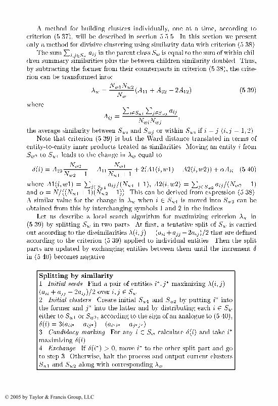
���� EXTENSIONS TO OTHER DATA TYPES ���
A method for building clusters individually� one at a time� according tocriterion ������� will be described in section ������ In this section we presentonly a method for divisive clustering using similarity data with criterion �������The sum
Pi�j�Sw
aij in the parent class Sw is equal to the sum of within children summary similarities plus the between children similarity doubled� Thus�by subtracting the former from their counterparts in criterion ������� the criterion can be transformed into�
w �Nw�Nw�
Nw�A�� !A�� � �A��� ������
where
Aij �
Pi�Swi
Pj�Swj
aij
NwiNwj�
the average similarity between Swi and Swj or within Swi if i � j �i� j � �� ���Note that criterion ������ is but the Ward distance translated in terms of
entitytoentity inner products treated as similarities� Moving an entity i fromSw� to Sw� leads to the change in w equal to
��i� � A��Nw�
Nw� � � �A��Nw�
Nw� ! �! ��A��i� w���A��i� w��� ! �Aii ������
where A��i� w�� �P
j�Sw�aij��Nw� ! ��� A��i� w�� �
Pj�Sw�
aij��Nw� � ��and � � N���Nw� !���Nw� � ���� This can be derived from expression �������A similar value for the change in w when i � Sw� is moved into Sw� can beobtained from this by interchanging symbols � and � in the indices�Let us describe a local search algorithm for maximizing criterion w in
������ by splitting Sw in two parts� At rst� a tentative split of Sw is carriedout according to the dissimilarities �i� j� � �aii!ajj��aij��� that are denedaccording to the criterion ������ applied to individual entities� Then the splitparts are updated by exchanging entities between them until the increment �in ������ becomes negative�
Splitting by similarity�� Initial seeds� Find a pair of entities i�� j� maximizing �i� j� ��aii ! ajj � �aij��� over i� j � Sw��� Initial clusters� Create initial Sw� and Sw� by putting i
� intothe former and j� into the latter and by distributing each i � Sweither to Sw� or Sw�� according to the sign of an analogue to ���������i� � ��aii� � aij��� �ai�i� � aj�j����� Candidacy marking� For any i � Sw calculate ��i� and take i
�
maximizing ��i���� Exchange� If ��i�� � �� move i� to the other split part and goto step �� Otherwise� halt the process and output current clustersSw� and Sw� along with corresponding w�
© 2005 by Taylor & Francis Group, LLC
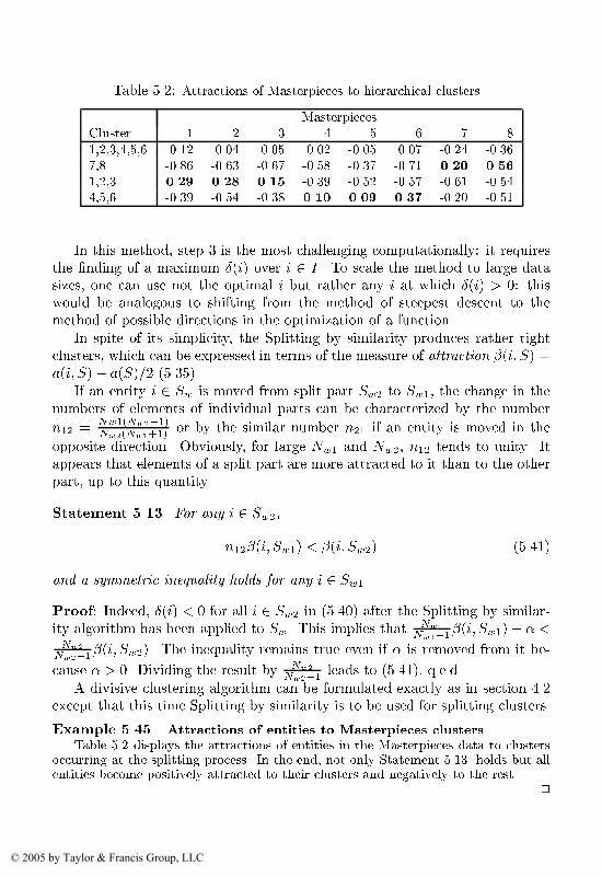
��� DATA RECOVERY MODELS
Table ���� Attractions of Masterpieces to hierarchical clusters�
MasterpiecesCluster � � � � � � � �
������ ��� �� �� �� ��� �� ���� ������ ���� ���� ���� ���� ���� ���� ���� ���
��� ���� ���� ��� ���� ���� ���� ���� ������� ���� ���� ���� ���� ���� ���� ��� ����
In this method� step � is the most challenging computationally� it requiresthe nding of a maximum ��i� over i � I � To scale the method to large datasizes� one can use not the optimal i but rather any i at which ��i� � �� thiswould be analogous to shifting from the method of steepest descent to themethod of possible directions in the optimization of a function�In spite of its simplicity� the Splitting by similarity produces rather tight
clusters� which can be expressed in terms of the measure of attraction ��i� S� �a�i� S�� a�S��� �������If an entity i � Sw is moved from split part Sw� to Sw�� the change in the
numbers of elements of individual parts can be characterized by the number
n�� �Nw��Nw����Nw��Nw����
or by the similar number n�� if an entity is moved in the
opposite direction� Obviously� for large Nw� and Nw�� n�� tends to unity� Itappears that elements of a split part are more attracted to it than to the otherpart� up to this quantity�
Statement ����� For any i � Sw��
n����i� Sw�� � ��i� Sw�� ������
and a symmetric inequality holds for any i � Sw��
Proof� Indeed� ��i� � � for all i � Sw� in ������ after the Splitting by similarity algorithm has been applied to Sw� This implies that
Nw�
Nw�����i� Sw�� ! � �
Nw�
Nw�����i� Sw��� The inequality remains true even if � is removed from it be
cause � � �� Dividing the result by Nw�
Nw���leads to ������� q�e�d�
A divisive clustering algorithm can be formulated exactly as in section ���except that this time Splitting by similarity is to be used for splitting clusters�
Example ����� Attractions of entities to Masterpieces clusters
Table ��� displays the attractions of entities in the Masterpieces data to clustersoccurring at the splitting process� In the end not only Statement ����� holds but allentities become positively attracted to their clusters and negatively to the rest�
�
© 2005 by Taylor & Francis Group, LLC
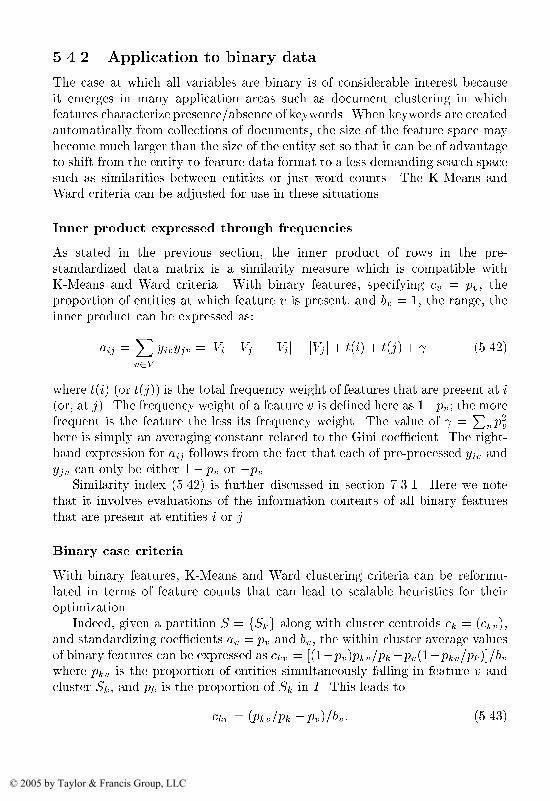
���� EXTENSIONS TO OTHER DATA TYPES ���
����� Application to binary data
The case at which all variables are binary is of considerable interest becauseit emerges in many application areas such as document clustering in whichfeatures characterize presence�absence of keywords� When keywords are createdautomatically from collections of documents� the size of the feature space maybecome much larger than the size of the entity set so that it can be of advantageto shift from the entitytofeature data format to a less demanding search spacesuch as similarities between entities or just word counts� The KMeans andWard criteria can be adjusted for use in these situations�
Inner product expressed through frequencies
As stated in the previous section� the inner product of rows in the prestandardized data matrix is a similarity measure which is compatible withKMeans and Ward criteria� With binary features� specifying cv � pv� theproportion of entities at which feature v is present� and bv � �� the range� theinner product can be expressed as�
aij �Xv�V
yivyjv � jVi � Vj j � jVij � jVj j! t�i� ! t�j� ! � ������
where t�i� �or t�j�� is the total frequency weight of features that are present at i�or� at j�� The frequency weight of a feature v is dened here as ��pv� the morefrequent is the feature the less its frequency weight� The value of � �
Pv p
�v
here is simply an averaging constant related to the Gini coe�cient� The righthand expression for aij follows from the fact that each of preprocessed yiv andyjv can only be either �� pv or �pv�Similarity index ������ is further discussed in section ������ Here we note
that it involves evaluations of the information contents of all binary featuresthat are present at entities i or j�
Binary case criteria
With binary features� KMeans and Ward clustering criteria can be reformulated in terms of feature counts that can lead to scalable heuristics for theiroptimization�Indeed� given a partition S � fSkg along with cluster centroids ck � �ckv��
and standardizing coe�cients av � pv and bv� the within cluster average valuesof binary features can be expressed as ckv � ����pv�pkv�pk�pv���pkv�pk���bvwhere pkv is the proportion of entities simultaneously falling in feature v andcluster Sk� and pk is the proportion of Sk in I � This leads to
ckv � �pkv�pk � pv��bv� ������
© 2005 by Taylor & Francis Group, LLC
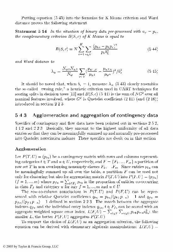
��� DATA RECOVERY MODELS
Putting equation ������ into the formulas for KMeans criterion and Warddistance proves the following statement�
Statement ����� In the situation of binary data pre�processed with av � pv�the complementary criterion B�S� c� of K�Means is equal to
B�S� c� � N
KXk��
Xv�V
�pkv � pkpv��
pkb�v������
and Ward distance to
w �Nw�Nw�
Nw
Xv�V
�pw��vpw�
� pw��vpw�
���b�v ������
It should be noted that� when bv � �� measure w ������ closely resemblesthe socalled �twoing rule�� a heuristic criterion used in CART techniques forscoring splits in decision trees ���� and B�S� c� ������ is the sum of NG� over allnominal features involved� where G� is Quetelet coe�cient ������ �and �������introduced in section ������
����� Agglomeration and aggregation of contingency data
Specics of contingency and �ow data have been pointed out in sections ����������� and ������ Basically� they amount to the highest uniformity of all dataentries so that they can be meaningfully summed up and naturally preprocessedinto Quetelet association indexes� These specics are dwelt on in this section�
Agglomeration
Let P �T� U� � �ptu� be a contingency matrix with rows and columns representing categories t � T and u � U � respectively� and F � fF�� ���� Fmg a partition ofrow set T in nonoverlapping nonempty classes F�� ����Fm� Since entries ptu canbe meaningfully summed up all over the table� a partition F can be used notonly for clustering but also for aggregating matrix P �T� U� into P �F�U� � �pfu��f � �� ����m� where pfu �
Pt�Ff
ptu is the proportion of entities cooccurringin class Ff and category u for any f � �� ����m and u � U �The rowtocolumn associations in P �T� U� and P �F�U� can be repre
sented with relative Quetelet coe�cients qtu � ptu��pt�p�u� � � and qfu �pfu��pf�p�u� � � dened in section ������ The match between the aggregateindexes qfu and the individual entry indexes qtu� t � Ff � can be scored with anaggregate weighted square error index� L�F�U� �
Pt�T
Pu�U pt�p�ue
�tu� the
smaller L� the better P �F�U� aggregates P �T� U��To support the choice of L�F�U� as an aggregation criterion� the following
equation can be derived with elementary algebraic manipulations� L�F�U� �
© 2005 by Taylor & Francis Group, LLC
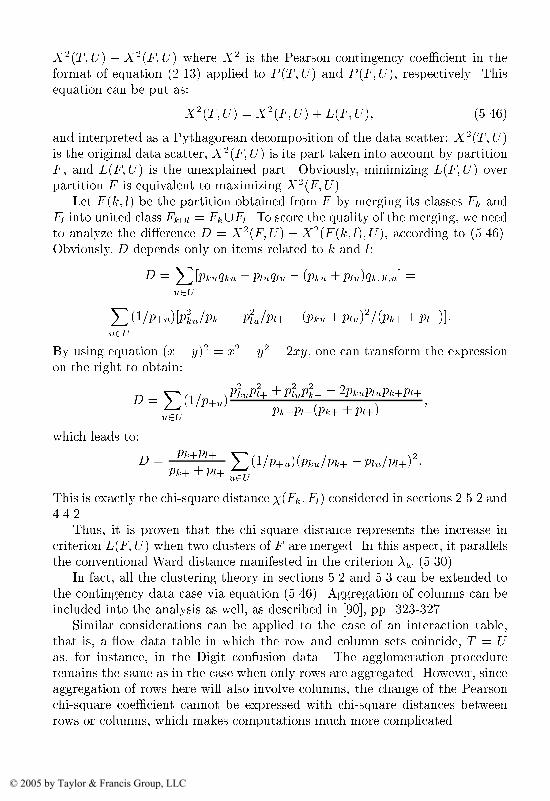
���� EXTENSIONS TO OTHER DATA TYPES ���
X��T� U� � X��F�U� where X� is the Pearson contingency coe�cient in theformat of equation ������ applied to P �T� U� and P �F�U�� respectively� Thisequation can be put as�
X��T� U� � X��F�U� ! L�F�U�� ������
and interpreted as a Pythagorean decomposition of the data scatter� X��T� U�is the original data scatter� X��F�U� is its part taken into account by partitionF � and L�F�U� is the unexplained part� Obviously� minimizing L�F�U� overpartition F is equivalent to maximizing X��F�U��Let F �k� l� be the partition obtained from F by merging its classes Fk and
Fl into united class Fk�l � Fk�Fl� To score the quality of the merging� we needto analyze the di erence D � X��F�U� �X��F �k� l�� U�� according to �������Obviously� D depends only on items related to k and l�
D �Xu�U
�pkuqku ! pluqlu � �pku ! plu�qk�l�u� �
Xu�U
���p�u��p�ku�pk� ! p�lu�pl� � �pku ! plu�
���pk� ! pl����
By using equation �x� y�� � x� ! y� � �xy� one can transform the expressionon the right to obtain�
D �Xu�U
���p�u�p�kup
�l� ! p�lup
�k� � �pkuplupk�pl�
pk�pl��pk� ! pl���
which leads to�
D �pk�pl�
pk� ! pl�
Xu�U
���p�u��pku�pk� � plu�pl����
This is exactly the chisquare distance ��Fk � Fl� considered in sections ����� and������Thus� it is proven that the chisquare distance represents the increase in
criterion L�F�U� when two clusters of F are merged� In this aspect� it parallelsthe conventional Ward distance manifested in the criterion w �������In fact� all the clustering theory in sections ��� and ��� can be extended to
the contingency data case via equation ������� Aggregation of columns can beincluded into the analysis as well� as described in ����� pp� �������Similar considerations can be applied to the case of an interaction table�
that is� a �ow data table in which the row and column sets coincide� T � Uas� for instance� in the Digit confusion data� The agglomeration procedureremains the same as in the case when only rows are aggregated� However� sinceaggregation of rows here will also involve columns� the change of the Pearsonchisquare coe�cient cannot be expressed with chisquare distances betweenrows or columns� which makes computations much more complicated�
© 2005 by Taylor & Francis Group, LLC
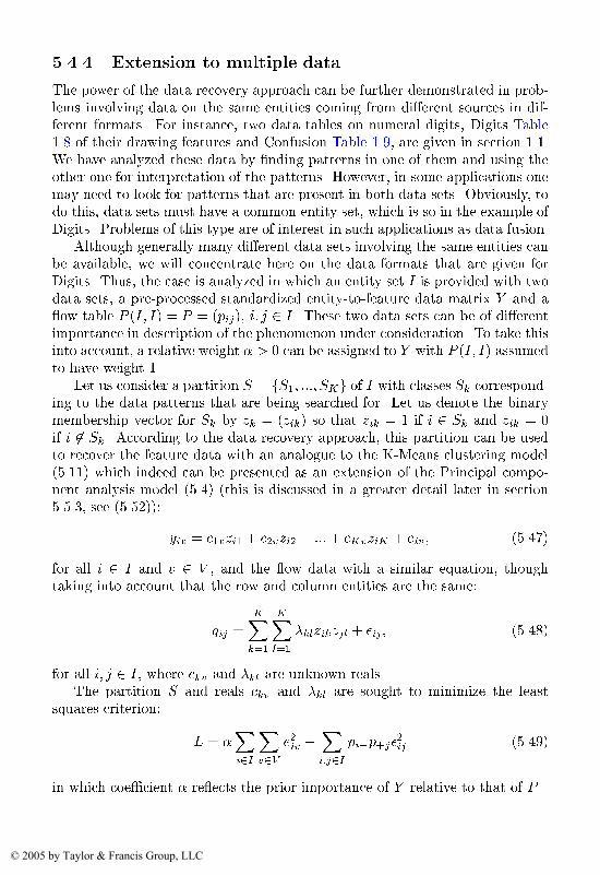
��� DATA RECOVERY MODELS
����� Extension to multiple data
The power of the data recovery approach can be further demonstrated in problems involving data on the same entities coming from di erent sources in different formats� For instance� two data tables on numeral digits� Digits Table��� of their drawing features and Confusion Table ���� are given in section ����We have analyzed these data by nding patterns in one of them and using theother one for interpretation of the patterns� However� in some applications onemay need to look for patterns that are present in both data sets� Obviously� todo this� data sets must have a common entity set� which is so in the example ofDigits� Problems of this type are of interest in such applications as data fusion�Although generally many di erent data sets involving the same entities can
be available� we will concentrate here on the data formats that are given forDigits� Thus� the case is analyzed in which an entity set I is provided with twodata sets� a preprocessed standardized entitytofeature data matrix Y and a�ow table P �I� I� � P � �pij�� i� j � I � These two data sets can be of di erentimportance in description of the phenomenon under consideration� To take thisinto account� a relative weight � � � can be assigned to Y with P �I� I� assumedto have weight ��Let us consider a partition S � fS�� ���� SKg of I with classes Sk correspond
ing to the data patterns that are being searched for� Let us denote the binarymembership vector for Sk by zk � �zik� so that zik � � if i � Sk and zik � �if i � Sk� According to the data recovery approach� this partition can be usedto recover the feature data with an analogue to the KMeans clustering model������ which indeed can be presented as an extension of the Principal component analysis model ����� �this is discussed in a greater detail later in section������ see ��������
yiv � c�vzi� ! c�vzi� ! ���! cKvziK ! eiv � ������
for all i � I and v � V � and the �ow data with a similar equation� thoughtaking into account that the row and column entities are the same�
qij �
KXk��
KXl��
klzikzjl ! �ij � ������
for all i� j � I � where ckv and kl are unknown reals�The partition S and reals ckv and kl are sought to minimize the least
squares criterion�
L � �Xi�I
Xv�V
e�iv !Xi�j�I
pi�p�j��ij ������
in which coe�cient � re�ects the prior importance of Y relative to that of P �
© 2005 by Taylor & Francis Group, LLC
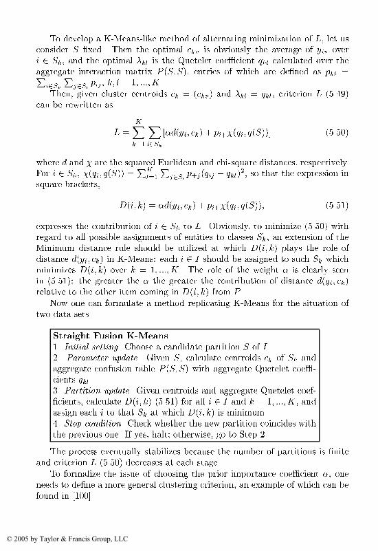
���� EXTENSIONS TO OTHER DATA TYPES ���
To develop a KMeanslike method of alternating minimization of L� let usconsider S xed� Then the optimal ckv is obviously the average of yiv overi � Sk� and the optimal kl is the Quetelet coe�cient qkl calculated over theaggregate interaction matrix P �S� S�� entries of which are dened as pkl �P
i�Sk
Pj�Sl
pij � k� l � �� ����K�
Then� given cluster centroids ck � �ckv� and kl � qkl� criterion L ������can be rewritten as
L �
KXk��
Xi�Sk
��d�yi� ck� ! pi���qi� q�S��� ������
where d and � are the squared Euclidean and chisquare distances� respectively�For i � Sk� ��qi� q�S�� �
PKl��
Pj�Sl
p�j�qij � qkl��� so that the expression in
square brackets�
D�i� k� � �d�yi� ck� ! pi���qi� q�S��� ������
expresses the contribution of i � Sk to L� Obviously� to minimize ������ withregard to all possible assignments of entities to classes Sk� an extension of theMinimum distance rule should be utilized at which D�i� k� plays the role ofdistance d�yi� ck� in KMeans� each i � I should be assigned to such Sk whichminimizes D�i� k� over k � �� ����K� The role of the weight � is clearly seenin ������� the greater the � the greater the contribution of distance d�yi� ck�relative to the other item coming in D�i� k� from P �Now one can formulate a method replicating KMeans for the situation of
two data sets�
Straight Fusion K�Means�� Initial setting� Choose a candidate partition S of I ��� Parameter update� Given S� calculate centroids ck of Sk andaggregate confusion table P �S� S� with aggregate Quetelet coe�cients qkl��� Partition update� Given centroids and aggregate Quetelet coefcients� calculate D�i� k� ������ for all i � I and k � �� ����K� andassign each i to that Sk at which D�i� k� is minimum��� Stop condition� Check whether the new partition coincides withthe previous one� If yes� halt� otherwise� go to Step ��
The process eventually stabilizes because the number of partitions is niteand criterion L ������ decreases at each stage�To formalize the issue of choosing the prior importance coe�cient �� one
needs to dene a more general clustering criterion� an example of which can befound in ������
© 2005 by Taylor & Francis Group, LLC
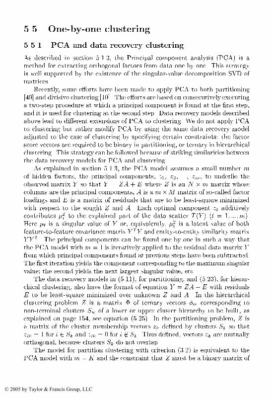
��� DATA RECOVERY MODELS
��� One�by�one clustering
����� PCA and data recovery clustering
As described in section ������ the Principal component analysis �PCA� is amethod for extracting orthogonal factors from data one by one� This strategyis well supported by the existence of the singularvalue decomposition SVD ofmatrices�Recently� some e orts have been made to apply PCA to both partitioning
���� and divisive clustering ����� The e orts are based on consecutively executinga twostep procedure at which a principal component is found at the rst step�and it is used for clustering at the second step� Data recovery models describedabove lead to di erent extensions of PCA to clustering� We do not apply PCAto clustering but rather modify PCA by using the same data recovery modeladjusted to the case of clustering by specifying certain constraints� the factorscore vectors are required to be binary in partitioning� or ternary in hierarchicalclustering� This strategy can be followed because of striking similarities betweenthe data recovery models for PCA and clustering�As explained in section ������ the PCA model assumes a small number m
of hidden factors� the principal components� z�� z�� ���� zm� to underlie theobserved matrix Y so that Y � ZA ! E where Z is an N m matrix whosecolumns are the principal components� A is a mM matrix of socalled factorloadings and E is a matrix of residuals that are to be leastsquare minimizedwith respect to the sought Z and A� Each optimal component zt additivelycontributes ��t to the explained part of the data scatter T �Y � �t � �� ����m��Here �t is a singular value of Y or� equivalently� ��t is a latent value of bothfeaturetofeature covariance matrix Y TY and entitytoentity similarity matrixY Y T � The principal components can be found one by one in such a way thatthe PCA model with m � � is iteratively applied to the residual data matrix Yfrom which principal components found at previous steps have been subtracted�The rst iteration yields the component corresponding to the maximum singularvalue� the second yields the next largest singular value� etc�The data recovery models in ������� for partitioning� and ������� for hierar
chical clustering� also have the format of equation Y � ZA!E with residualsE to be leastsquare minimized over unknown Z and A� In the hierarchicalclustering problem Z is a matrix ' of ternary vectors �w corresponding tononterminal clusters Sw of a lower or upper cluster hierarchy to be built� asexplained on page ���� see equation ������� In the partitioning problem� Z isa matrix of the cluster membership vectors zk dened by clusters Sk so thatzik � � for i � Sk and zik � � for i � Sk� Thus dened� vectors zk are mutuallyorthogonal� because clusters Sk do not overlap�The model for partition clustering with criterion ����� is equivalent to the
PCA model with m � K and the constraint that Z must be a binary matrix of
© 2005 by Taylor & Francis Group, LLC

���� ONE�BY�ONE CLUSTERING ���
the cluster membership vectors� Similarly� the model for hierarchical clusteringis equivalent to the PCA model with the restriction that Z must be a matrix ofm ternary split membership vectors� The PCA strategy of extracting columnsof Z one by one� explained in section ������ thus can be applied in each of thesesituations� We begin by describing an adaptation of this strategy to the case ofhierarchical clustering and then to the case of partitioning� Extensions to thesimilarity and contingency data are brie�y described next �for more detail� see������
����� Divisive Wardlike clustering
Given an upper cluster hierarchy S � fSwg� each item cw� � cw in equation������ with cw� being the centroid of Sw� � S and cw the centroid of the parentSw� contributes w � wd�Sw�� Sw�� �
Nw�Nw�
Nwd�cw�� cw�� ������ to data scatter
T �Y � according to equation ������� This implies that� to build S � fSwgfrom scratch� that is� by starting from the universal cluster Sw � I � one canemploy the PCA onebyone strategy by adding to S one split at a time� eachtime maximizing contribution w of the split to the explained part of the datascatter so that w plays the role of the squared singular value �
�t of Y � The
analogy is not supercial� Both �t andpw express the scaling coe�cient
when projecting the data onto a corresponding axis which follows the principalcomponent zt� for the former� and the ternary split vector �w� for the latter�In the sequel to this section� we are going to demonstrate that the divisive
Wardlike algorithm described in section ��� is an implementation of the PCAonebyone extracting strategy� The strategy involves two types of iterations�One� major iteration� builds a series of splits of clusters Sw into split parts Sw�and Sw� to greedily maximize the summary contribution
PSw�S
w to the datascatter T �Y �� The other� minor iteration� is utilized when maximizing individual w by splitting Sw using a specic splitting method� Two such methodsdescribed in section ��� t into the strategy because they do maximize w�though locally� They are� a straight method� with �Means� and an incremental method� Splitting by separation� based on a di erent expression� ������ forw�The use of �Means with Euclidean squared distance d� not Ward distance
dw� for splitting is justied with the following statement�
Statement ����� The ��Means algorithm for splitting Sw maximizes �locallythe Ward distance between split parts�
Proof� According to equation ������� the criterion minimized in splitting ofpartition L�S� for an upper cluster hierarchy S by maximizing the Ward distance ������ is W �L�S�� c�L�S���� the KMeans criterion� q�e�d�Another proof of this statement is given in section ������
© 2005 by Taylor & Francis Group, LLC
��� DATA RECOVERY MODELS
Each splitting step is equivalent to nding a ternary splitting vector maximizing Ward distance between its parts or� equivalently� minimizing the summary squared residuals in ������ with regard to all possible tertiary columnvectors �w � ��iw� and any rowvectors aw � �awv� in model ������� Accordingto the rstorder optimality conditions� the optimal vector aw in ������ relatesto the �w as the weighted vector of di erences� awv �
pNw�Nw��Nw�cw��v �
cw��v�� which concurs with the data recovery model ������ for hierarchical clustering�
����� Iterated Anomalous pattern
In this section we are going to demonstrate that the PCA onebyone strategyapplied when the membership vectors are constrained to be binary� is but theiterated Anomalous pattern analysis�Consider a set of subsets Sk � I � each specied by a binary N dimensional
vector zk � �zik� where zik � � if i � Sk and zik � � if i � Sk� �Vector zk isinterpreted as the membership vector for subset Sk � I �� The data recoverymodel ������ for KMeans can be rewritten with zk in the following way�
yiv � c�vzi� ! c�vzi� ! ���! cKvziK ! eiv � ������
which follows the PCA model ����� with m � K factors and the additionalrequirement that scoring vectors zk must be binary�The onebyone extracting strategy here would require the building of clus
ters Sk one by one� each time minimizing criterion�
l �Xi�I
Xv�V
�yiv � cvzi�� ������
over unknown cv and binary zi� index k being omitted� The membership vectorz is characterized by subset S � fi � zi � �g� Criterion ������ can be rewrittenin terms of S� as follows�
W �S� c� �Xi�S
d�yi� c� !Xi��S
d�yi� �� ������
This is the square error criterion ����� for a partition consisting of twoclusters� S and its complement "S � I � S� with regard to their respectivecentroids� c and �� However� in contrast to the KMeans method� the centroid� here is not the center of gravity of the complementary set I � S� but is keptconstant and does not change when S and I � S change�Given S� the optimal c in ������ is obviously the center of gravity of S
because the rst sum is constant there� Given c� a subset S to minimize ������must include every i � I such that d�yi� c� � d�yi� ��� Obviously� these are
© 2005 by Taylor & Francis Group, LLC
���� ONE�BY�ONE CLUSTERING ���
exactly the rules in Steps � and � of the Anomalous pattern clustering algorithmin section ������Thus� the following is proven�
Statement ����� The Anomalous pattern algorithm iteratively minimizes����� according to the alternating optimization rule� given c� �nd optimal S�and given S� �nd optimal c� The initial choice of c in the Anomalous clusterminimizes ����� over all singleton clusters�
Thus� the AP method is a set of minor iterations of alternatingly optimizingcriterion ������ for selecting the best cluster�After one cluster has been found� the next one can be sought in the remain
der of the set I � to obtain a cluster partition � this amounts to the iteratedapplication of Anomalous pattern in Intelligent KMeans �section ����� Another version of the onebyone Anomalous clustering� with the residual datamatrix and not necessarily nonoverlapping clusters� is described in ����� section����
����� Anomalous pattern versus Splitting
A question related to the Anomalous pattern method is whether any relationexists between its criterion ������ and Ward criterion w� in its form ����� usedin the Splitting by separating algorithm� Both methods separate a cluster froma body of entities with a squareerror criterion�To analyze the situation at any of the major iterations� let us denote the
entity set under consideration by J � the separated cluster by S� with its centroidc�� Consider also a prespecied point c in J � which is the centroid of J in Wardclustering and a reference point in the Anomalous pattern clustering� The othersubset� J � S�� will be denoted by S�� In these denotations� the Anomalouspattern criterion can be expressed as�
W �Xi�S�
d�yi� c�� !Xi�S�
d�yi� c�
and the Ward splitting criterion as�
w �NJN�
N�d�c�� c�
where NJ � N� and N� are the sizes �cardinalities� of J � S� and S�� respectively�To analyze the relationship between these criteria� let us add to and sub
tract from W the complementary partP
i�S�d�yi� c�� Then W � T �Y� c� !P
i�S�d�yi� c�� �
Pi�S�
d�yi� c� where T �Y� c� denotes the sum of squared Euclidean distances from all points in J to c� that is� the scatter of the data
© 2005 by Taylor & Francis Group, LLC
��� DATA RECOVERY MODELS
around c� an item which is constant with respect to the cluster S� being separated� By noting that d�yi� c� � �yi� yi� ! �c� c� � ��yi� c� and d�yi� c�� ��yi� yi�! �c�� c��� ��yi� c��� the last expression can be equivalently rewritten asW � T �Y� c��N�d�c�� c�� The following is proven�
Statement ����� Both separating methods� Anomalous pattern and Splittingby separation� maximize the weighted distance �d�c�� c� between centroid c� ofthe cluster being separated and a pre�speci�ed point c� The di�erence betweenthe methods is that�
� the weight is � � N� in the Anomalous pattern and � � N��N� in theSplitting by separation� and
�� c is the user�speci�ed reference point in the former and the unvariedcentroid of set J being split in the latter�
The di erence ��� disappears if the reference point has been set at thecentroid of J � The di erence ��� is fundamental� as proven in section ������both sets� S� and S�� are tight clusters in Splitting� whereas only one of them�S�� is to be tight as the Anomalous pattern� the rest� J � S�� may be a set ofrather disconnected entities� This shows once again the e ect of size coe�cientsin cluster criteria�
����� Onebyone clusters for similarity data
Let A � �aij�� i� j � I � be a given similarity matrix and z��zizj� a weightedbinary matrix dened by a binary membership vector z � �zi� of a subsetS � fi � I � zi � �g along with its numeric intensity weight � When A can beconsidered as noisy information on a set of weighted �additive clusters� kzkz
Tk �
k � �� ���K� the following model can be assumed ������� ������
aij � �zi�zj� ! ���! mziKzjK ! eij ������
where eij are residuals to be minimized� According to model ������� similaritiesaij are dened by the intensity weights of clusters containing both i and j�Equations ������ must hold� generally� for each pair �i� j�� With no loss ofgenerality� we accept in this section that aij are symmetric and not dened ati � j so that only i � j are considered�In matrix terms� the model is A � Z&ZT !E where Z is an N K matrix
of cluster membership vectors� & is a K K diagonal matrix with ������ Kon its main diagonal� all other entries being zero� and E � �eij� the residualmatrix� In fact� this matrix equation is analogous to the socalled spectral� orlatent value� decomposition of a symmetric matrix A �����The onebyone PCA strategy suggests that� provided that A has been pre
liminarily centered� minimizing L�E� �P
i�j e�ij over unknown Sk and k�
k � �� ����K� can be done by nding one cluster S at a time to minimize
© 2005 by Taylor & Francis Group, LLC
���� ONE�BY�ONE CLUSTERING ���
L �P
i�j�I �aij�zizj�� with respect to all possible and binary z � �zi�� Obviously� given S � I � minimizing criterion L is the average similarity withincluster S� that is� � a�S� where a�S� �
Pi�j�S�i�j aij��jSj�jSj � ������ In
matrix terms� a�S� � zTAz�zTz�After a cluster S and corresponding � a�S� are found� similarities are
changed for residual similarities aij �zizj � and the process of nding a clusterS and its intensity a�S� is reiterated using the updated similarity matrix� Inthe case of nonoverlapping clusters� there is no need to calculate the residualsimilarity� the process needs only be applied to only those entities that haveremained as yet unclustered�When the clusters are assumed to be mutually nonoverlapping �that is� the
membership vectors zt are mutually orthogonal� or when tting of the model isdone using the onebyone PCA strategy� the data scatter decomposition holdsas follows �����
T �A� �
KXk��
�zTk Akzk�zTk zk�
� ! L�E� ������
in which the leastsquares optimal k�s are taken as the within cluster averagesof the �residual� similarities� The matrix Ak in ������ is either A unchanged�if clusters are not overlapping� or a residual similarity matrix at iteration k�Ak � A�Pk��
t�� kzkzTk �
Equation ������ shows that nding leastsquares optimal clusters requiresmaximizing the intermediate term in ������� which is the sum of squared criteria ������ or ������ discussed in section ������ When applying the onebyoneextraction strategy so that one cluster is sought at a time� the constituent onecluster criterion is the squared criterion ������� To nd a cluster optimizingit� one may exploit its square root� criterion ������ itself� which will be brie�ydiscussed next�In ���� ��� a number of incremental procedures to maximize A�S� ������ or
its square are described to involve the average similarity of an entity i � I to asubset S�
a�i� S� �Xj�S
aij�jSj ������
A very straightforward procedure for extracting a cluster� given a similaritymatrix A � �aij�� i� j � I is referred to as ADDIS in ����� The computationstarts at S consisting of just two entities� i� and j�� such that ai�j� is the maximum similarity in A� Given a current S� the procedure proceeds in calculatinga�i� S� for all i � I � both belonging to S and not� This can be done incrementally� Then a threshold � � a�S��� is calculated to select those i�s that satisfya�i� S� � �� this� basically� checks the signs of the attractions of entities to S�
© 2005 by Taylor & Francis Group, LLC
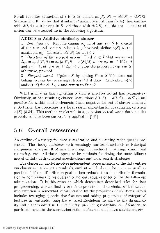
��� DATA RECOVERY MODELS
Recall that the attraction of i to S is dened as ��i� S� � a�i� S� � a�S����Statement ����� states that if subset S maximizes criterion ������ then entitieswith ��i� S� � � belong in S and those with ��i� S� � � do not� This line ofaction can be wrapped up in the following algorithm�
ADDI�S or Additive similarity cluster�� Initialization� Find maximum aij in A and set S to consistof the row and column indexes i� j involved� dene a�S� as themaximum aij � Calculate a�i� S� for all i � I ��� Direction of the steepest ascent� Find i� � I that maximizes%i� � si���i
�� S� � si��a�i�� S�� a�S���� where si� � �� if i � S
and si� � �� otherwise� If %i� � �� stop the process at current S�otherwise� proceed��� Steepest ascent� Update S by adding i� to S if it does notbelong to S or by removing it from S if it does� Recalculate a�S�and a�i� S� for all i � I and return to Step ��
What is nice in this algorithm is that it involves no ad hoc parameters�Obviously� at the resulting cluster� attractions ��i� S� � a�i� S� � a�S��� arepositive for withincluster elements i and negative for outofcluster elementsi� Actually� the procedure is a local search algorithm for maximizing criterionA�S� ������� This method works well in application to real world data� similarprocedures have been successfully applied in ������
�� Overall assessment
An outline of a theory for data visualization and clustering techniques is presented� The theory embraces such seemingly unrelated methods as Principalcomponent analysis� KMeans clustering� hierarchical clustering� conceptualclustering� etc� All these appear to be methods for tting the same bilinearmodel of data with di erent specications and local search strategies�
The clustering model involves independent representation of the data entriesvia cluster centroids with residuals� each of which should be made as small aspossible� This multicriterion goal is then reduced to a onecriterion formulation by combining the residuals into the least squares criterion for the followupminimization� It is this criterion which determines described rules for datapreprocessing� cluster nding and interpretation� The choice of the scalarized criterion is somewhat substantiated by the properties of solutions� whichinclude� averaging quantitative features and taking proportions of categoricalfeatures in centroids� using the squared Euclidean distance as the dissimilarity and inner product as the similarity� producing contributions of features topartitions equal to the correlation ratio or Pearson chisquare coe�cient� etc�
© 2005 by Taylor & Francis Group, LLC
��� OVERALL ASSESSMENT ���
The theory supports�
�� A unied framework for KMeans and Ward clustering that not only justies conventional partitioning and agglomerative methods but extendsthem to mixed scale and multiple table data�
�� Modied versions of the algorithms such as scalable divisive clustering aswell as intelligent versions of KMeans mitigating the need in userdrivenad hoc parameters�
�� Compatible measures and criteria for similarity data to produce provablytight clusters with the tightness measured by the attraction coe�cientderived in the data recovery framework�
�� E ective measures and clustering criteria for analyzing binary data tables�
�� Onebyone clustering procedures that allow for more �exible clusteringstructures including single clusters� overlapping clusters� and incompleteclustering�
�� Interpretation aids based on decompositions of the data scatter over elements of cluster structures to judge elements� relative contributions�
�� Conventional and modied measures of statistical association� such asthe correlation ratio and Pearson chisquare contingency coe�cient� assummary contributions of cluster structures to the data scatter�
�� A related framework for cluster analysis of contingency and �ow data inwhich the data scatter and contributions are measured in terms of thePearson chisquare contingency coe�cient�
© 2005 by Taylor & Francis Group, LLC
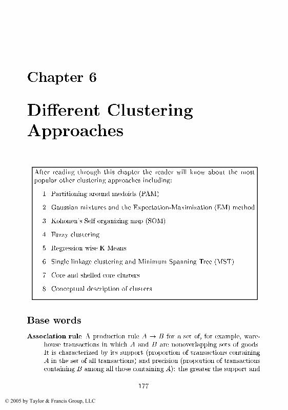
Chapter �
Di�erent Clustering
Approaches
After reading through this chapter the reader will know about the mostpopular other clustering approaches including�
�� Partitioning around medoids �PAM�
�� Gaussian mixtures and the ExpectationMaximization �EM� method
�� Kohonen�s Selforganizing map �SOM�
�� Fuzzy clustering
�� Regressionwise KMeans
�� Single linkage clustering and Minimum Spanning Tree �MST�
�� Core and shelled core clusters
�� Conceptual description of clusters
Base words
Association rule A production rule A � B for a set of� for example� warehouse transactions in which A and B are nonoverlapping sets of goods�It is characterized by its support �proportion of transactions containingA in the set of all transactions� and precision �proportion of transactionscontaining B among all those containing A�� the greater the support and
���
© 2005 by Taylor & Francis Group, LLC
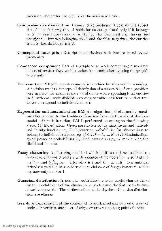
��� DIFFERENT CLUSTERING APPROACHES
precision� the better the quality of the association rule�
Comprehensive description A conjunctive predicate A describing a subsetS � I in such a way that A holds for an entity if and only if it belongsto S� It may have errors of two types� the false positives� the entitiessatisfying A but not belonging to S� and the false negatives� the entitiesfrom S that do not satisfy A�
Conceptual description Description of clusters with feature based logicalpredicates�
Connected component Part of a graph or network comprising a maximalsubset of vertices that can be reached from each other by using the graph�sedges only�
Decision tree A highly popular concept in machine learning and data mining�A decision tree is a conceptual description of a subset S � I or a partitionon I in a treelike manner� the root of the tree corresponding to all entitiesin I � with each node divided according to values of a feature so that treeleaves correspond to individual classes�
Expectation and maximization EM An algorithm of alternating maximization applied to the likelihood function for a mixture of distributionsmodel� At each iteration� EM is performed according to the followingsteps� ��� Expectation� Given parameters of the mixture pk and individual density functions ak� nd posterior probabilities for observations tobelong to individual clusters� gik �i � I� k � �� ����K�� ��� Maximization�given posterior probabilities gik� nd parameters pk� ak maximizing thelikelihood function�
Fuzzy clustering A clustering model at which entities i � I are assumed tobelong to di erent clusters k with a degree of membership zik so that ���
zik � � andPK
k�� zik � � for all i � I and k � �� ����K� Conventional�crisp� clusters can be considered a special case of fuzzy clusters in whichzik may only be � or ��
Gaussian distribution A popular probabilistic cluster model characterizedby the modal point of the cluster mean vector and the featuretofeaturecovariance matrix� The surfaces of equal density for a Gaussian distribution are ellipses�
Graph A formalization of the concept of network involving two sets� a set ofnodes� or vertices� and a set of edges or arcs connecting pairs of nodes�
© 2005 by Taylor & Francis Group, LLC
BASE WORDS ���
Medoid An entity in a cluster with the minimal summary distance to the otherwithin cluster elements� It is used as a formalization of the concept ofprototype in the PAM clustering method�
Minimum spanning tree A tree structure within a graph such that its summary edge weights are minimal� This concept is the backbone of themethod of single link clustering�
Mixture of distributions A probabilistic clustering model according towhich each cluster can be represented by a unimodal probabilistic densityfunction so that the population density is a probabilistic mixture of theindividual cluster functions� This concept integrates a number of simplermodels and algorithms for tting them� including the KMeans clusteringalgorithm� The assumptions leading to KMeans can be overly restrictive�such as the compulsory zscore data standardization�
Production rule A predicate A � B which is true for those and only thoseentities that either satisfy B whenever they satisfy A� A conceptual description of a cluster S can be a production rule A � B in which Bexpresses belongingness of an entity to S�
Regression�wise clustering A clustering model in which a cluster is soughtas a set of observations satisfying a regression function� Such a model canbe tted with an extension of KMeans in which prototypes are presentedas regression functions�
Self�organizing map A model for data visualization in the form of a grid onplane in which entities are represented by grid nodes re�ecting both theirsimilarity and the grid topology�
Shelled core A clustering model according to which the data are organized asa dense core surrounded by shells of a lesser density�
Single link clustering A method in clustering in which the betweenclusterdistance is dened by the nearest entities� The method is related to theminimum spanning trees and connected components in the correspondinggraphs�
Weakest link partitioning A method for sequentially removing �weakestlink� entities from the data set� Thus found series is utilized for nding the shelled core�
© 2005 by Taylor & Francis Group, LLC
��� DIFFERENT CLUSTERING APPROACHES
�� Extensions of K�Means clustering
����� Clustering criteria and implementation
Traditionally� a cluster is understood as a subset of entities which are similarto each other and dissimilar from the rest� However� in realworld situationsadditional properties may be required which may complement and sometimeseven contradict this view� Consider� for instance� a set of young men withonly one variable� their height� measured� Depending on our perspective� wemay be interested in the deviate clusters of those who are too short or tootall to carry out regular sailor duties� or rather in the central core cluster ofthose who normally t them� The issue of denition of what is a central corecluster becomes less trivial when encountered in the setting of a webbased orother network� Dening what is a deviate cluster can be of issue in specicsettings such as dealing with banking customers� Extending the men�s heightexample to a mixed sex group� one might be interested in dening clustersof male and female individuals in terms of probabilistic normal distributionswith di ering means and variances� which is a traditional abstraction for heightmeasure on humans� A di erent clustering goal invites a di erent formalizationand di erent methods for clustering�In Chapter �� a number of userdened goals for clustering were described�
These goals typically cannot be explicitly formalized and� thus� are implicit inclustering methods� The explicit goals are much more technical and down toearth� In particular� criteria optimized by KMeans and Ward methods aresuch that the found clusters�
�� consist of entities that are the most similar to each other and their centroids�
�� are the most associated with features involved in the data�
�� are the most anomalous and thus interesting�
These claims can be supported with materials in sections ������ ����� and ����respectively� A review of related clustering methods emerging in the context ofdata compression is given in ������The goals above obviously could be pursued with di erently dened con
cepts of distance �dissimilarity�� centroid and correlation� Even within the datarecovery approach� di erent approximation criteria would lead to di erentlydened distances and centroids within the goal ��� of the list above� If� for example� the quality of the data recovery is scored with the sum of moduli� ratherthan squares� of di erences between the original and recovered data� then thecorresponding distance between entities x � �x�� ���� xm� and y � �y�� ���� yM �is measured by the sum of moduli� d �
Pv jxv � yvj� not the sum of squares�
© 2005 by Taylor & Francis Group, LLC
��� EXTENSIONS OF K�MEANS CLUSTERING ���
This distance is frequently used in data analysis and referred to as Manhattan distance or cityblock metric� Within the data recovery approach with theleastmoduli criterion the concept of centroid would slightly change too� it isthe medians� not the averages that would populate them# Both Manhattandistance and medianbased centroids bring more stability to cluster solutions�especially with respect to outliers� However� the very same stability propertiescan make leastmoduli based datarecovery clustering less versatile with respectto the presence of mixed scale data �����One may use di erent distance and centroid concepts with computational
schemes of KMeans and hierarchical clustering without any strictly denedmodel framework as� for instance� proposed in ����� A popular method fromthat book� PAM �Partitioning around medoids�� will be described in the nextsubsection�There can be other clustering goals as well� In particular� the following are
rather popular�
I Cluster membership of an entity may not necessarily be conned to onecluster only but shared among several clusters �Fuzzy clustering��
II Geometrically� cluster shapes may be not necessarily spherical as in theclassic KMeans but may have shapes elongated along regression lines�Regressionwise clustering��
III Data may come from a probabilistic distribution which is a mixture ofunimodal distributions that are to be separated to represent di erentclusters �Expectation�Maximization method EM��
IV A visual representation of clusters on a twodimensional screen can beexplicitly embedded in clustering �SelfOrganizing Map method SOM��
Further on in this section we present extensions of KMeans clustering techniques that are oriented towards these goals�
����� Partitioning around medoids PAM
KMeans centroids are average points rather than individual entities� whichmay be considered too articial in some clustering problems in which the usermay wish to involve nothing articial but only genuinely occurring entities� Toimplement this idea� let us change the concept of a cluster�s centroid for thatof a cluster�s medoid� An entity of a cluster S� i� � S� will be referred to asits medoid if it minimizes the sum of distances to other elements of S� that is�P
j�S d�i�� j� � mini�S
Pj�S d�i� j�� The symbol d�i� j� is used here to denote
a dissimilarity function� not necessarily squared Euclidean distance� betweenentities i� j � I �
© 2005 by Taylor & Francis Group, LLC
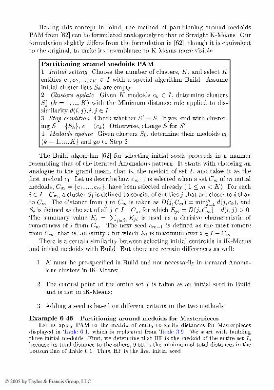
��� DIFFERENT CLUSTERING APPROACHES
Having this concept in mind� the method of partitioning around medoidsPAM from ���� can be formulated analogously to that of Straight KMeans� Ourformulation slightly di ers from the formulation in ����� though it is equivalentto the original� to make its resemblance to KMeans more visible�
Partitioning around medoids PAM�� Initial setting� Choose the number of clusters� K� and select Kentities c�� c�� ���� cK � I with a special algorithm Build� Assumeinitial cluster lists Sk are empty��� Clusters update� Given K medoids ck � I � determine clustersS�k �k � �� ����K� with the Minimum distance rule applied to dissimilarity d�i� j�� i� j � I ��� Stop�condition� Check whether S� � S� If yes� end with clustering S � fSkg� c � �ck�� Otherwise� change S for S���� Medoids update� Given clusters Sk� determine their medoids ck�k � �� ����K� and go to Step ��
The Build algorithm ���� for selecting initial seeds proceeds in a mannerresembling that of the iterated Anomalous pattern� It starts with choosing ananalogue to the grand mean� that is� the medoid of set I � and takes it as therst medoid c�� Let us describe how cm�� is selected when a set Cm of m initialmedoids� Cm � fc�� ���� cmg� have been selected already � � � m � K�� For eachi � I�Cm� a cluster Si is dened to consist of entities j that are closer to i thanto Cm� The distance from j to Cm is taken as D�j� Cm� � min
mk�� d�j� ck�� and
Si is dened as the set of all j � I�Cm for which Eji � D�j� Cm��d�i� j� � ��The summary value Ei �
Pj�Si
Eji is used as a decisive characteristic ofremoteness of i from Cm� The next seed cm�� is dened as the most remotefrom Cm� that is� an entity i for which Ei is maximum over i � I � Cm�There is a certain similarity between selecting initial centroids in iKMeans
and initial medoids with Build� But there are certain di erences as well�
�� K must be prespecied in Build and not necessarily in iterated Anomalous clusters in iKMeans�
�� The central point of the entire set I is taken as an initial seed in Buildand is not in iKMeans�
�� Adding a seed is based on di erent criteria in the two methods�
Example ����� Partitioning around medoids for Masterpieces
Let us apply PAM to the matrix of entity�to�entity distances for Masterpiecesdisplayed in Table ��� which is replicated from Table ���� We start with buildingthree initial medoids� First we determine that HF is the medoid of the entire set Ibecause its total distance to the others ��� is the minimum of total distances in thebottom line of Table ���� Thus HF is the �rst initial seed�
© 2005 by Taylor & Francis Group, LLC
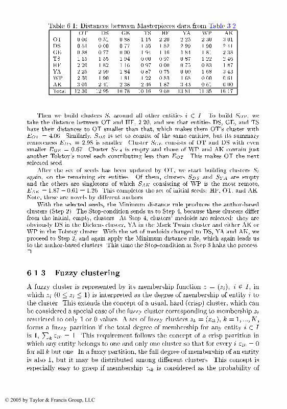
��� EXTENSIONS OF K�MEANS CLUSTERING ���
Table ���� Distances between Masterpieces data from Table ����OT DS GE TS HF YA WP AK
OT ���� ���� ���� ���� ���� ���� ���� ����DS ���� ���� ���� ���� ���� �� ��� ���GE ���� ���� ���� �� ���� ��� ���� ����TS ���� ���� �� ���� ��� ���� ���� ���HF ���� ���� ���� ��� ���� ���� ���� ����YA ���� �� ��� ���� ���� ���� ���� ���WP ���� ��� ���� ���� ���� ���� ���� ����AK ���� ��� ���� ��� ���� ��� ���� ����Total ����� ���� ����� ����� ��� ����� ����� �����
Then we build clusters Si around all other entities i � I� To build SOT wetake the distance between OT and HF ��� and see that entities DS GE and TShave their distances to OT smaller than that which makes them OT�s cluster withEOT � ���� Similarly SDS is set to consist of the same entities but its summaryremoteness EDS � ���� is smaller� Cluster SGE consists of OT and DS with evensmaller EGE � ���� Cluster SY A is empty and those of WP and AK contain justanother Tolstoy�s novel each contributing less than EOT � This makes OT the nextselected seed�
After the set of seeds has been updated by OT we start building clusters Siagain on the remaining six entities� Of them clusters SDS and SY A are emptyand the others are singletons of which SAK consisting of WP is the most remoteEAK � ���� � ��� � ����� This completes the set of initial seeds� HF OT and AK�Note these are novels by di�erent authors�
With the selected seeds the Minimum distance rule produces the author�basedclusters �Step � � The Stop�condition sends us to Step � because these clusters di�erfrom the initial empty clusters� At Step � clusters� medoids are selected� they areobviously DS in the Dickens cluster YA in the Mark Twain cluster and either AK orWP in the Tolstoy cluster� With the set of medoids changed to DS YA and AK weproceed to Step � and again apply the Minimum distance rule which again leads usto the author�based clusters� This time the Stop�condition at Step � halts the process��
����� Fuzzy clustering
A fuzzy cluster is represented by its membership function z � �zi�� i � I� inwhich zi �� � zi � �� is interpreted as the degree of membership of entity i tothe cluster� This extends the concept of a usual� hard �crisp� cluster� which canbe considered a special case of the fuzzy cluster corresponding to membership zirestricted to only � or � values� A set of fuzzy clusters zk � �zik�� k � �� ����K�forms a fuzzy partition if the total degree of membership for any entity i � Iis ��
Pk zik � �� This requirement follows the concept of a crisp partition in
which any entity belongs to one and only one cluster so that for every i zik � �for all k but one� In a fuzzy partition� the full degree of membership of an entityis also �� but it may be distributed among di erent clusters� This concept isespecially easy to grasp if membership zik is considered as the probability of
© 2005 by Taylor & Francis Group, LLC
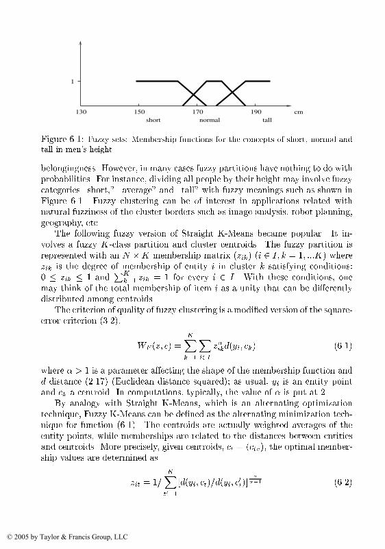
��� DIFFERENT CLUSTERING APPROACHES
cm150 170 190short normal tall
1
130
Figure ���� Fuzzy sets� Membership functions for the concepts of short normal andtall in men�s height�
belongingness� However� in many cases fuzzy partitions have nothing to do withprobabilities� For instance� dividing all people by their height may involve fuzzycategories �short�� �average� and �tall� with fuzzy meanings such as shown inFigure ���� Fuzzy clustering can be of interest in applications related withnatural fuzziness of the cluster borders such as image analysis� robot planning�geography� etc�The following fuzzy version of Straight KMeans became popular� It in
volves a fuzzy Kclass partition and cluster centroids� The fuzzy partition isrepresented with an N K membership matrix �zik� �i � I� k � �� ���K� wherezik is the degree of membership of entity i in cluster k satisfying conditions�� � zik � � and
PKk�� zik � � for every i � I � With these conditions� one
may think of the total membership of item i as a unity that can be di erentlydistributed among centroids�The criterion of quality of fuzzy clustering is a modied version of the square
error criterion ������
WF �z� c� �
KXk��
Xi�I
z�ikd�yi� ck� �����
where � � � is a parameter a ecting the shape of the membership function andd distance ������ �Euclidean distance squared�� as usual� yi is an entity pointand ck a centroid� In computations� typically� the value of � is put at ��By analogy with Straight KMeans� which is an alternating optimization
technique� Fuzzy KMeans can be dened as the alternating minimization technique for function ������ The centroids are actually weighted averages of theentity points� while memberships are related to the distances between entitiesand centroids� More precisely� given centroids� ct � �ctv�� the optimal membership values are determined as
zit � ��
KXt���
�d�yi� ct��d�yi� c�t��
���� �����
© 2005 by Taylor & Francis Group, LLC
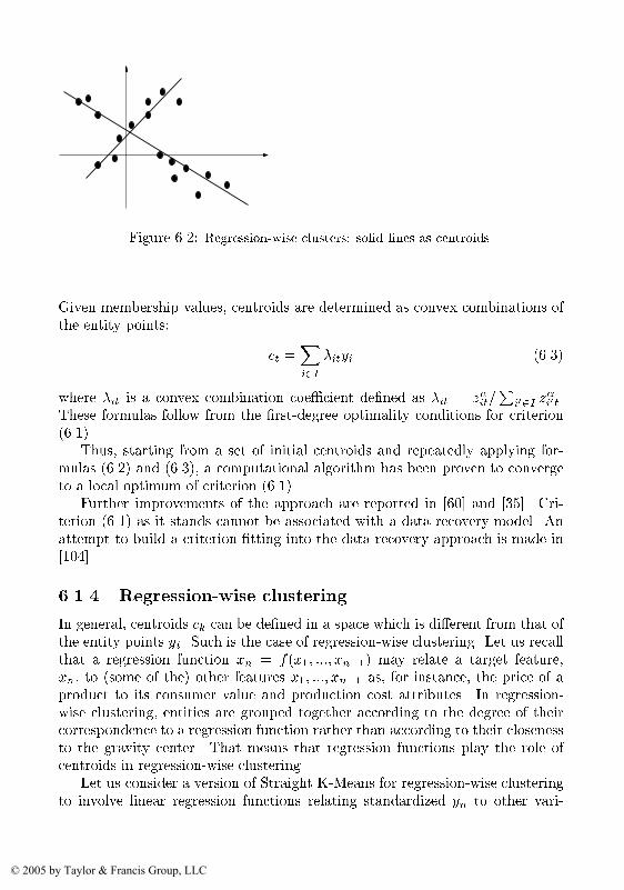
��� EXTENSIONS OF K�MEANS CLUSTERING ���
Figure ���� Regression�wise clusters� solid lines as centroids�
Given membership values� centroids are determined as convex combinations ofthe entity points�
ct �Xi�I
ityi �����
where it is a convex combination coe�cient dened as it � z�it�P
i��I z�i�t�
These formulas follow from the rstdegree optimality conditions for criterion������Thus� starting from a set of initial centroids and repeatedly applying for
mulas ����� and ������ a computational algorithm has been proven to convergeto a local optimum of criterion ������Further improvements of the approach are reported in ���� and ����� Cri
terion ����� as it stands cannot be associated with a data recovery model� Anattempt to build a criterion tting into the data recovery approach is made in������
����� Regressionwise clustering
In general� centroids ck can be dened in a space which is di erent from that ofthe entity points yi� Such is the case of regressionwise clustering� Let us recallthat a regression function xn � f�x�� ���� xn��� may relate a target feature�xn� to �some of the� other features x�� ���� xn�� as� for instance� the price of aproduct to its consumer value and production cost attributes� In regressionwise clustering� entities are grouped together according to the degree of theircorrespondence to a regression function rather than according to their closenessto the gravity center� That means that regression functions play the role ofcentroids in regressionwise clustering�Let us consider a version of Straight KMeans for regressionwise clustering
to involve linear regression functions relating standardized yn to other vari
© 2005 by Taylor & Francis Group, LLC
��� DIFFERENT CLUSTERING APPROACHES
ables� y�� ���� yn��� in each cluster� Such a function is dened by the equationyn � a�y� ! a�y� ! ��� ! an��yn�� ! a for some coe�cients a� a�� ���� an���These coe�cients form a vector� a � �a� a�� ���� an���� which can be referred to as the regressionwise centroid� When a regressionwise centroid isgiven� its distance to an entity point yi � �yi�� ���� yin� is dened as r�i� a� ��yin � a�yi� � a�yi� � ��� � an��yi�n�� � a�
�� the squared di erence betweenthe observed value of yn and that calculated from the regression equation� Todetermine the regressionwise centroid a�S�� given a cluster list S � I � the standard technique of multivariate linear regression analysis is applied� which is butminimizing the within cluster summary residual
Pi�S r�i� a� over all possible
a�
Then Straight KMeans can be applied with the only changes being that���� centroids must be regressionwise centroids and ��� the entitytocentroiddistance must be r�i� a��
����� Mixture of distributions and EM algorithm
Data of nancial transactions or astronomic observations can be considered asa random sample from a �potentially� innite population� In such cases� thedata structure can be analyzed with probabilistic approaches of which arguablythe most radical is the mixture of distributions approach�
According to this approach� each of the yet unknown clusters k is modeled bya density function f�x� ak� which represents a family of density functions over xdened up to a parameter vector ak� A onedimensional density function f�x��for any small dx � �� assigns probability f�x�dx to the interval between x andx! dx� multidimensional density functions have similar interpretation�
Usually� the density f�x� ak� is considered unimodal �the mode corresponding to a cluster standard point�� such as the normal� or Gaussian� density function dened by its mean vector �k and covariance matrix (k�
f�x� ak� � ��p�pj(kj����� expf��x� �k�
T(��k �x� �k���g �����
The shape of Gaussian clusters is ellipsoidal because any surface at whichf�x� ak� ����� is constant satises equation �x��k�T(��k �x��k� � const deningan ellipsoid� The mean vector �k species the kth cluster�s location�
The mixture of distributions clustering model can be set as follows� Therow points y�� ���� yN are considered a random sample of jV jdimensional observations from a population with density function f�x� which is a mixture of individual cluster density functions f�x� ak� �k � �� ����K� so that
f�x� �PK
k�� pkf�x� ak� where pk � � are the mixture probabilities�P
k pk � ��For f�x� ak� being the normal density� ak � ��k�(k� where �k is the mean and(k the covariance matrix�
© 2005 by Taylor & Francis Group, LLC
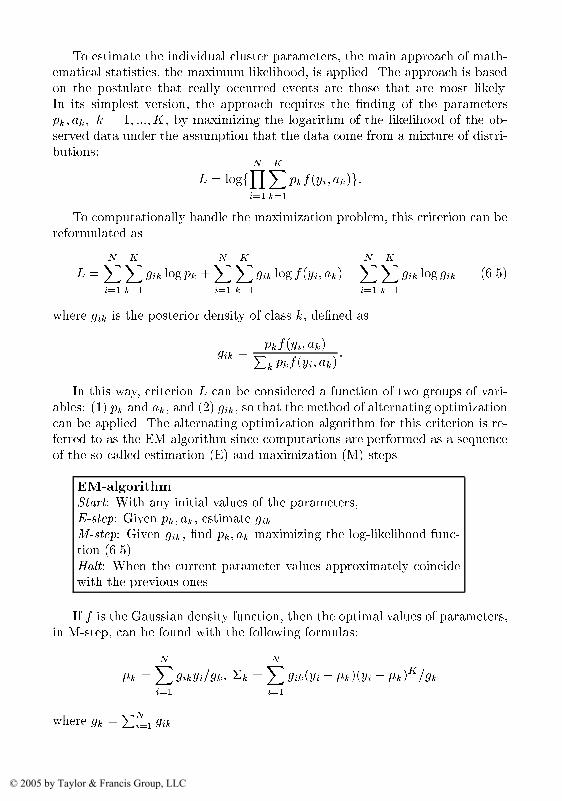
��� EXTENSIONS OF K�MEANS CLUSTERING ���
To estimate the individual cluster parameters� the main approach of mathematical statistics� the maximum likelihood� is applied� The approach is basedon the postulate that really occurred events are those that are most likely�In its simplest version� the approach requires the nding of the parameterspk� ak� k � �� ����K� by maximizing the logarithm of the likelihood of the observed data under the assumption that the data come from a mixture of distributions�
L � logfNYi��
KXk��
pkf�yi� ak�g�
To computationally handle the maximization problem� this criterion can bereformulated as
L �
NXi��
KXk��
gik log pk !
NXi��
KXk��
gik log f�yi� ak��NXi��
KXk��
gik log gik �����
where gik is the posterior density of class k� dened as
gik �pkf�yi� ak�Pk pkf�yi� ak�
�
In this way� criterion L can be considered a function of two groups of variables� ��� pk and ak� and ��� gik� so that the method of alternating optimizationcan be applied� The alternating optimization algorithm for this criterion is referred to as the EMalgorithm since computations are performed as a sequenceof the socalled estimation �E� and maximization �M� steps�
EM�algorithmStart� With any initial values of the parameters�E�step� Given pk� ak� estimate gik�M�step� Given gik� nd pk� ak maximizing the loglikelihood function ������Halt� When the current parameter values approximately coincidewith the previous ones�
If f is the Gaussian density function� then the optimal values of parameters�in Mstep� can be found with the following formulas�
�k �
NXi��
gikyi�gk� (k �
NXi��
gik�yi � �k��yi � �k�K�gk
where gk �PN
i�� gik�
© 2005 by Taylor & Francis Group, LLC
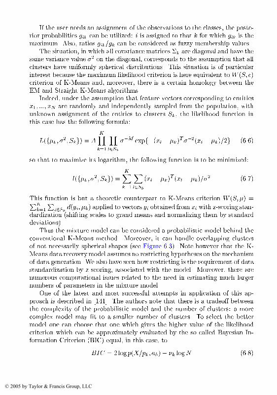
��� DIFFERENT CLUSTERING APPROACHES
If the user needs an assignment of the observations to the classes� the posterior probabilities gik can be utilized� i is assigned to that k for which gik is themaximum� Also� ratios gik�gk can be considered as fuzzy membership values�The situation� in which all covariance matrices (k are diagonal and have the
same variance value � on the diagonal� corresponds to the assumption that allclusters have uniformly spherical distributions� This situation is of particularinterest because the maximum likelihood criterion is here equivalent to W �S� c�criterion of KMeans and� moreover� there is a certain homology between theEM and Straight KMeans algorithms�Indeed� under the assumption that feature vectors corresponding to entities
x�� ���� xN are randomly and independently sampled from the population� withunknown assignment of the entities to clusters Sk� the likelihood function inthis case has the following formula�
L�f�k� �� Skg� � A
KYk��
Yi�Sk
�M expf��xi � �k�T ���xi � �k���g �����
so that to maximize its logarithm� the following function is to be minimized�
l�f�k� �� Skg� �KXk��
Xi�Sk
�xi � �k�T �xi � �k��
� �����
This function is but a theoretic counterpart to KMeans criterion W �S� �� �PKk��
Pi�Sk
d�yi� �k� applied to vectors yi obtained from xi with zscoring standardization �shifting scales to grand means and normalizing them by standarddeviations��Thus the mixture model can be considered a probabilistic model behind the
conventional KMeans method� Moreover� it can handle overlapping clustersof not necessarily spherical shapes �see Figure ����� Note however that the KMeans data recoverymodel assumes no restricting hypotheses on the mechanismof data generation� We also have seen how restricting is the requirement of datastandardization by zscoring� associated with the model� Moreover� there arenumerous computational issues related to the need in estimating much largernumbers of parameters in the mixture model�One of the latest and most successful attempts in application of this ap
proach is described in ������ The authors note that there is a tradeo betweenthe complexity of the probabilistic model and the number of clusters� a morecomplex model may t to a smaller number of clusters� To select the bettermodel one can choose that one which gives the higher value of the likelihoodcriterion which can be approximately evaluated by the so called Bayesian Information Criterion �BIC� equal� in this case� to
BIC � � log p�X�pk� ak�� �k logN �����
© 2005 by Taylor & Francis Group, LLC
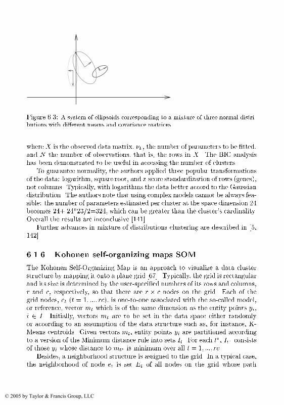
��� EXTENSIONS OF K�MEANS CLUSTERING ���
Figure ���� A system of ellipsoids corresponding to a mixture of three normal distri�butions with di�erent means and covariance matrices�
where X is the observed data matrix� �k� the number of parameters to be tted�and N the number of observations� that is� the rows in X � The BIC analysishas been demonstrated to be useful in accessing the number of clusters�To guarantee normality� the authors applied three popular transformations
of the data� logarithm� square root� and zscore standardization of rows �genes��not columns� Typically� with logarithms the data better accord to the Gaussiandistribution� The authors note that using complex models cannot be always feasible� the number of parameters estimated per cluster at the space dimension ��becomes ��! ��)��������� which can be greater than the cluster�s cardinality�Overall the results are inconclusive ������Further advances in mixture of distributions clustering are described in ���
�����
����� Kohonen selforganizing maps SOM
The Kohonen SelfOrganizing Map is an approach to visualize a data clusterstructure by mapping it onto a plane grid ����� Typically� the grid is rectangularand its size is determined by the userspecied numbers of its rows and columns�r and c� respectively� so that there are r c nodes on the grid� Each of thegrid nodes� et �t � �� ���� rc�� is onetoone associated with the socalled model�or reference� vector mt which is of the same dimension as the entity points yi�i � I � Initially� vectors mt are to be set in the data space either randomlyor according to an assumption of the data structure such as� for instance� KMeans centroids� Given vectors mt� entity points yi are partitioned accordingto a version of the Minimum distance rule into sets It� For each t
�� It� consistsof those yi whose distance to mt� is minimum over all t � �� ���� rc�Besides� a neighborhood structure is assigned to the grid� In a typical case�
the neighborhood of node et is set Et of all nodes on the grid whose path
© 2005 by Taylor & Francis Group, LLC
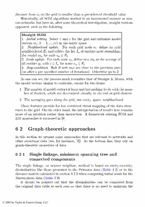
��� DIFFERENT CLUSTERING APPROACHES
distance from et on the grid is smaller than a preselected threshold value�Historically� all SOM algorithms worked in an incremental manner as neu
ron networks� but later on� after some theoretical investigation� straight versionsappeared� such as the following�
Straight SOM�� Initial setting� Select r and c for the grid and initialize modelvectors mt �t � �� ���� rc� in the entity space��� Neighborhood update� For each grid node et� dene its gridneighborhood Et and collect the list Iu of entities most resemblingthe model mu for each eu � Et��� Seeds update� For each node et� dene new mt as the average ofall entities yi with i � Iu for some eu � Et��� Stop�condition� Halt if new mts are close to the previous ones�or after a prespecied number of iterations�� Otherwise go to ��
As one can see� the process much resembles that of Straight KMeans� withthe model vectors similar to centroids� except for two items�
�� The number of model vectors is large and has nothing to do with the number of clusters� which are determined visually in the end as grid clusters�
�� The averaging goes along the grid� not entity space� neighborhood�
These features provide for less restricted visual mapping of the data structures to the grid� On the other hand� the interpretation of results here remainsmore of an intuition rather than instruction� A framework relating SOM andEM approaches is proposed in ����
�� Graph�theoretic approaches
In this section we present some approaches that are relevant to networks andother structural data �see� for instance� ����� As the bottom line� they rely ongraphtheoretic properties of data�
����� Single linkage� minimum spanning tree andconnected components
The single linkage� or nearest neighbor� method is based on entitytoentitydissimilarities like those presented in the Primates data �Table ���� or in thedistance matrix calculated in section ����� when computing initial seeds for theMasterpieces data �Table �����It should be pointed out that the dissimilarities can be computed from
the original data table at each step so that there is no need to maintain the
© 2005 by Taylor & Francis Group, LLC
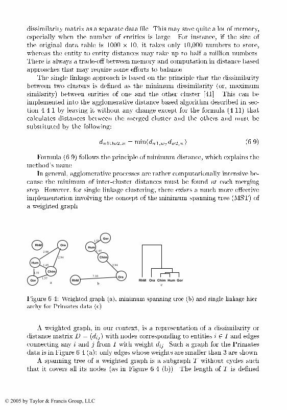
��� GRAPH�THEORETIC APPROACHES ���
dissimilarity matrix as a separate data le� This may save quite a lot of memory�especially when the number of entities is large� For instance� if the size ofthe original data table is ���� ��� it takes only ������ numbers to store�whereas the entitytoentity distances may take up to half a million numbers�There is always a tradeo between memory and computation in distance basedapproaches that may require some e orts to balance�The single linkage approach is based on the principle that the dissimilarity
between two clusters is dened as the minimum dissimilarity �or� maximumsimilarity� between entities of one and the other cluster ����� This can beimplemented into the agglomerative distance based algorithm described in section ����� by leaving it without any change except for the formula ������ thatcalculates distances between the merged cluster and the others and must besubstituted by the following�
dw��w��w � min�dw��w� dw��w� �����
Formula ����� follows the principle of minimum distance� which explains themethod�s name�In general� agglomerative processes are rather computationally intensive be
cause the minimum of intercluster distances must be found at each mergingstep� However� for single linkage clustering� there exists a much more e ectiveimplementation involving the concept of the minimum spanning tree �MST� ofa weighted graph�
RhM Ora Chim Hum Gorc
Gor
Ora
1.51
1.45
2.94
7.10
RhM
Chim
Hum
b
Chim
2.98
2.94
1.45
1.51
1.57
Ora
Hum
Gor
RhM
a
Figure ���� Weighted graph �a minimum spanning tree �b and single�linkage hier�archy for Primates data �c �
A weighted graph� in our context� is a representation of a dissimilarity ordistance matrix D � �dij� with nodes corresponding to entities i � I and edgesconnecting any i and j from I with weight dij � Such a graph for the Primatesdata is in Figure ��� �a�� only edges whose weights are smaller than � are shown�A spanning tree of a weighted graph is a subgraph T without cycles such
that it covers all its nodes �as in Figure ��� �b��� The length of T is dened
© 2005 by Taylor & Francis Group, LLC
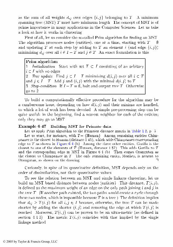
��� DIFFERENT CLUSTERING APPROACHES
as the sum of all weights dij over edges fi� jg belonging to T � A minimumspanning tree �MST� T must have minimum length� The concept of MST is ofprime importance in many applications in the Computer Sciences� Let us takea look at how it works in clustering�
First of all� let us consider the socalled Prim algorithm for nding an MST�The algorithm processes nodes �entities�� one at a time� starting with T � �and updating T at each step by adding to T an element i �and edge fi� jg�minimizing dij over all i � I � T and j � T � An exact formulation is this�
Prim algorithm�� Initialization� Start with set T � I consisting of an arbitaryi � I with no edges��� Tree update� Find j � I � T minimizing d�i� j� over all i � Tand j � I � T � Add j and �i� j� with the minimal d�i� j� to T ��� Stop�condition� If I�T � �� halt and output tree T � Otherwisego to ��
To build a computationally e ective procedure for the algorithm may bea cumbersome issue� depending on how d�i� j� and their minima are handled�to which a lot of work has been devoted� A simple preprocessing step can bequite useful� in the beginning� nd a nearest neighbor for each of the entities�only they may go to MST�
Example ����� Building MST for Primate data
Let us apply Prim algorithm to the Primates distance matrix in Table ��� p� ��Let us start for instance with T� fHumang� Among remaining entities Chim�
panzee is the closest to Human �distance ���� which adds Chimpanzee correspondingedge to T as shown in Figure ��� �b � Among the three other entities Gorilla is theclosest to one of the elements of T �Human distance ���� � This adds Gorilla to Tand the corresponding edge in MST in Figure ��� �b � Then comes Orangutan asthe closest to Chimpanzee in T � The only remaining entity Monkey is nearest toOrangutan as shown on the drawing� �
Curiously� in spite of its quantitative denition� MST depends only on theorder of dissimilarities� not their quantitative values�
To see the relation between an MST and single linkage clustering� let usbuild an MST based distance between nodes �entities�� This distance� T �i� j��is dened as the maximum weight of an edge on the only path joining i and j inthe tree T � �If another path existed� the two paths would create a cycle throughthese two nodes� which is impossible because T is a tree�� The denition impliesthat dij � T �i� j� for all i� j � I because� otherwise� the tree T can be madeshorter by adding the shorter �i� j� and removing the edge at which T �i� j� isreached� Moreover� T �i� j� can be proven to be an ultrametric �as dened insection ������� The metric T �i� j� coincides with that implied by the singlelinkage method�
© 2005 by Taylor & Francis Group, LLC
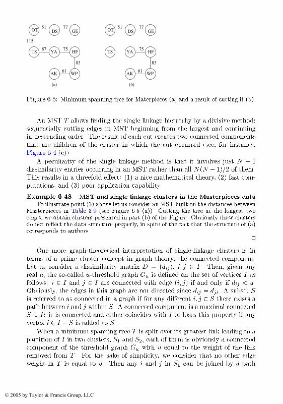
��� GRAPH�THEORETIC APPROACHES ���
OT GE
AK WP
YA HFTS
DS51 77
115
87 75
83
61
OT GE
AK WP
YA HFTS
DS51 77
75
83
61
(a) (b)
Figure ���� Minimum spanning tree for Materpieces �a and a result of cutting it �b �
An MST T allows nding the single linkage hierarchy by a divisive method�sequentially cutting edges in MST beginning from the largest and continuingin descending order� The result of each cut creates two connected componentsthat are children of the cluster in which the cut occurred �see� for instance�Figure ��� �c���
A peculiarity of the single linkage method is that it involves just N � �dissimilarity entries occurring in an MST rather than all N�N � ���� of them�This results in a threefold e ect� ��� a nice mathematical theory� ��� fast computations� and ��� poor application capability�
Example ����� MST and single linkage clusters in the Masterpieces data
To illustrate point �� above let us consider an MST built on the distances betweenMasterpieces in Table ��� �see Figure ��� �a � Cutting the tree at the longest twoedges we obtain clusters presented in part �b of the Figure� Obviously these clustersdo not re"ect the data structure properly in spite of the fact that the structure of �a corresponds to authors�
�
One more graphtheoretical interpretation of singlelinkage clusters is interms of a prime cluster concept in graph theory� the connected component�Let us consider a dissimilarity matrix D � �dij�� i� j � I � Then� given anyreal u� the socalled uthreshold graph Gu is dened on the set of vertices I asfollows� i � I and j � I are connected with edge �i� j� if and only if dij � u�Obviously� the edges in this graph are not directed since dij � dji� A subset Sis referred to as connected in a graph if for any di erent i� j � S there exists apath between i and j within S� A connected component is a maximal connectedS � I � it is connected and either coincides with I or loses this property if anyvertex i � I � S is added to S�
When a minimum spanning tree T is split over its greatest link leading to apartition of I in two clusters� S� and S�� each of them is obviously a connectedcomponent of the threshold graph Gu with u equal to the weight of the linkremoved from T � For the sake of simplicity� we consider that no other edgeweight in T is equal to u� Then any i and j in S� can be joined by a path
© 2005 by Taylor & Francis Group, LLC
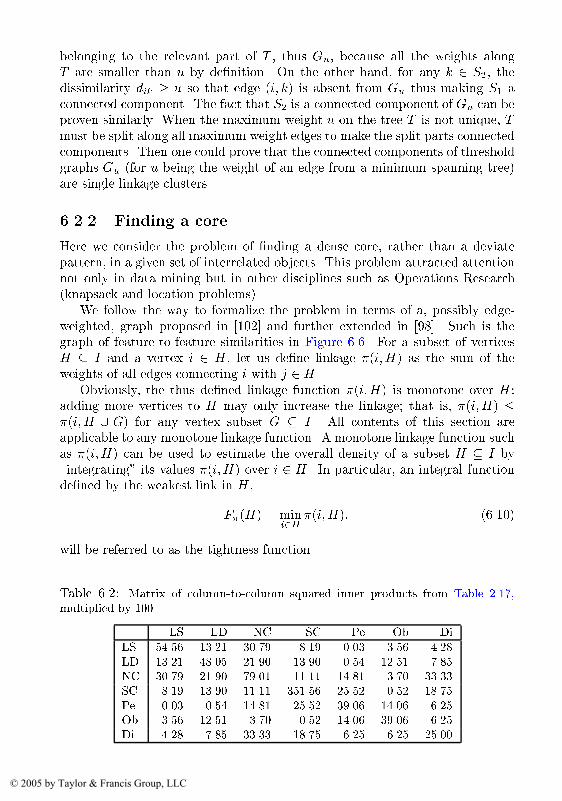
��� DIFFERENT CLUSTERING APPROACHES
belonging to the relevant part of T � thus Gu� because all the weights alongT are smaller than u by denition� On the other hand� for any k � S�� thedissimilarity dik � u so that edge �i� k� is absent from Gu thus making S� aconnected component� The fact that S� is a connected component of Gu can beproven similarly� When the maximum weight u on the tree T is not unique� Tmust be split along all maximum weight edges to make the split parts connectedcomponents� Then one could prove that the connected components of thresholdgraphs Gu �for u being the weight of an edge from a minimum spanning tree�are single linkage clusters�
����� Finding a core
Here we consider the problem of nding a dense core� rather than a deviatepattern� in a given set of interrelated objects� This problem attracted attentionnot only in data mining but in other disciplines such as Operations Research�knapsack and location problems��We follow the way to formalize the problem in terms of a� possibly edge
weighted� graph proposed in ����� and further extended in ����� Such is thegraph of featuretofeature similarities in Figure ���� For a subset of verticesH � I and a vertex i � H � let us dene linkage ��i�H� as the sum of theweights of all edges connecting i with j � H �Obviously� the thus dened linkage function ��i�H� is monotone over H �
adding more vertices to H may only increase the linkage� that is� ��i�H� ���i�H � G� for any vertex subset G � I � All contents of this section areapplicable to any monotone linkage function� A monotone linkage function suchas ��i�H� can be used to estimate the overall density of a subset H � I by�integrating� its values ��i�H� over i � H � In particular� an integral functiondened by the weakest link in H �
F��H� � mini�H
��i�H�� ������
will be referred to as the tightness function�
Table ���� Matrix of column�to�column squared inner products from Table ����multiplied by ��
LS LD NC SC Pe Ob Di
LS ����� ����� ���� ���� �� ���� ����LD ����� ���� ���� ���� ��� ����� ����NC ���� ���� ���� ����� ����� ��� �����SC ���� ���� ����� ������ ����� ��� �����Pe �� ��� ����� ����� ���� ���� ����Ob ���� ����� ��� ��� ���� ���� ����Di ���� ���� ����� ����� ���� ���� ���
© 2005 by Taylor & Francis Group, LLC
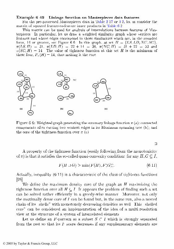
��� GRAPH�THEORETIC APPROACHES ���
Example ����� Linkage function on Masterpieces data featuresFor the pre�processed Masterpieces data in Table ���� or ��� let us consider the
matrix of squared feature�to�feature inner products in Table ����This matrix can be used for analysis of interrelations between features of Mas�
terpieces� In particular let us draw a weighted similarity graph whose vertices arefeatures and whose edges correspond to those similarities which are in the roundedform �� or greater see Figure ���� In this graph at set H � fLS� LD�NC� SCg��LS�H � �� ��LD�H � �� � �� � �� ��NC�H � �� � �� � �� and��SC�H � ��� The value of tightness function at this set H is the minimum ofthese four F��H � �� thus making it the core�
31
33
22
15
19
31
3333
19
(a) (b) (c)
LD
ObSC
NCNC
LS
NC
Di
LD
SCOb
Pe
LS
LD
SC
NC
Di
Ob
Pe
14
14
26 2626
15
22
Figure ���� Weighted graph generating the summary linkage function � �a � connectedcomponents after cutting two weakest edges in its Maximum spanning tree �b � andthe core of the tightness function over � �c �
�
A property of the tightness function �easily following from the monotonicityof �� is that it satises the socalled quasiconvexity condition� for anyH�G � I �
F �H �G� � min�F �H�� F �G��� ������
Actually� inequality ������ is a characteristic of the class of tightness functions�����We dene the maximum density core of the graph as H maximizing the
tightness function over all H � I � It appears the problem of nding such a setcan be solved rather e�ciently in a greedywise manner� Moreover� not onlythe maximally dense core of I can be found but� in the same run� also a nestedchain of its �shells� with monotonely decreasing densities as well� This �shelledcore� can be considered an implementation of the idea of a multiresolutionview at the structure of a system of interrelated elements�Let us dene an F pattern as a subset S � I which is strongly separated
from the rest so that its F score decreases if any supplementary elements are
© 2005 by Taylor & Francis Group, LLC
��� DIFFERENT CLUSTERING APPROACHES
added� even if some of its elements are removed� that is� F �S� � F �H� for anyH � I such that H � �I � S� � ��Thus dened� F patterns must be chainnested�
Statement ����� The set of all F �patterns� P � is nonempty and chain�nested�that is� S� � S� or S� � S� for any S�� S� � P �
Proof� If S�� S� are F patterns and S� is not part of S�� then F �S�� � F �F���If� moreover� S� is not part of S�� then F �S�� � F �S��� The contradictionproves that P must be chainnested� Besides� S � I makes the denition ofF pattern true because of the false premise� which proves that I is always anF pattern and completes the proof� q�e�d�In general� more dense subparts may occur within the smallest F pattern S�
nothing prevents one or more H � S with F �H� � F �S� to exist� When this isnot the case� that is� when the smallest F pattern is a global maximizer of thefunction F � the set of F patterns will be referred to as a layered cluster� whichis uniquely dened and thus can be considered as an aggregate representationof the F density structure in I �
Statement ����� If F �S� is a tightness function� then its minimum pattern isthe largest global maximizer of F �S� in the set of all S � I�
Proof� Let S be the minimum F pattern in the chain nested set of F patterns�If S is not a global maximizer of F � then F �H� � F �S� for some H � I � Infact� all such H must fall within S� because of the denition of F patterns� Letus take a maximal subset H � S in the set of all H such that F �H� � F �S�and prove that H is a pattern as well� Indeed� let us take any S� � S such thatS� � �I �H� � �� the existence of such S� follows from the fact that H does notcoincide with S� Then F �H� � F �H � S�� because of the assumed maximalityof H within S� But F �H � S�� � min�F �S��� F �H�� according to ������� thatis� F �H� � F �S��� Let us consider now an S� which is not contained in S andstill satises the condition S� � �I �H� � �� �This may only happen when S isnot equal to I �� By the denition of S�� F �S� � F �S�� because S is a pattern�Therefore� F �H� � F �S��� This implies that H is a pattern� which contradictsthe assumption of minimality of S� Thus� no H � S exists with F �H� � F �S�and S is the maximum global maximizer of F �H�� q�e�d�Let us denote by m�H� the �weakest link�� that is� the set of elements i � H
at which the value of F �H� is reached�
m�H� � fi � ��i�H� � minj�H
��j�H�g�
Obviously� m�H� is not empty if H is not empty� Iteratively applying theoperation m to I � I �m�I�� etc�� one can build a series of weakest links thatwill be referred to as the weakest link partition of I �
© 2005 by Taylor & Francis Group, LLC
��� CONCEPTUAL DESCRIPTION OF CLUSTERS ���
Weakest Link Partitioning�Input� Monotone linkage function ��i�H� dened for all pairs i�Hsuch that i � H � I �Output� Weakest link partition M � �M�M�� ����Mn� of I alongwith class values F �M� � fF� F�� ���� Fng dened as follows�Step �� Initial setting� Put t � � and dene I � I �Step �� Partitioning� Find class Mt � m�It� and dene It�� �It �Mt� Dene class value Ft � F��It� � ��i� It� for i �Mt�Step �� Stop�condition� If It�� � �� halt� Otherwise� add � to tand go to Step ��
The layered cluster of F patterns can be easily extracted from the weakestlink partition M thus produced�From the sequence F � pick up the smallest index t� among those maximizing
Ft� t � �� �� ���� n� Then apply the same selection rule to the starting partof the sequence F � F t� � �F� ���� Ft���� obtained by removing Ft� and allthe consequent elements� Reiterating this pickandremoval process until allelements of F are removed� we obtain set T � of all the picked up indices�Sets It� � t
� � T �� form the layered cluster of F�� which is proven in �����
Example ���� Building shelled core over featuresLet us apply the Weakest link partitioning algorithm to the graph in Figure ���
with linkage function ��i� S �P
j�S aij with aij being the weight� Obviously m�I �
fObg because ��Ob� I � �� is the minimum of ��i� I over all i � I� With theweakest link Ob removed from I the minimum of ��i� I � fObg is reached at LSwith ��LS� I � fObg � �� which is the next weakest link to be removed� The nextentity to be removed is LD with ��LD� I � fOb� LSg � ��� In the remaining setI� � fNC�Di� SC� Peg the weakest link is Pe with ��Pe� fNC�Di� SC� Peg � ���This yields I� � fNC�Di� SCg with the minimum link �� reached at m�I� � fSCg�Two remaining entities NC and Di are linked by ��� The results can be representedas a labeled sequence�
�Ob ���LS ���LD ���Pe ���SC ���Di�NC ���
where the parentheses contain sets Mt � m�It removed at each step of the algorithmtheir order re"ecting the order of removals� The labels correspond to the values ofthe linkage function F��It for t � � �� �� �� �� �� The maxima are �� �� �� ���the corresponding patterns being H� � fNC�Di� SC� Peg �part �c on Figure ��� H� � H� � fLDg H� � H� � fLSg and H� � I to form the layered cluster�
It should be noted that this drastically di�ers from any partition along the maxi�mum spanning tree presented in part �b of Figure ���� �
�� Conceptual description of clusters
Interpretation of clusters can be done at the following three levels� ��� clusterrepresentative� ��� statistical description� and ��� conceptual description� Of
© 2005 by Taylor & Francis Group, LLC
��� DIFFERENT CLUSTERING APPROACHES
these� we considered ��� and ��� in the previous chapters� Here we concentrateon the conceptual description of clusters�
����� False positives and negatives
A conceptual description of a cluster is a logic predicate over features denedon entities� that is� in general� true on entities belonging to the cluster andfalse on entities out of it� For instance� the cluster of Dickens masterpieces�according to Masterpieces data in Table ���� can be described conceptuallywith predicate �SCon��� or predicate ��� � LSent � �� * � � NChar � ���These descriptions can be tested for any entity from the table� Obviously� theformer predicate distinctively describes the cluster with no errors at all� whilethe latter admits one false positive error� the entity HuckFinn satises thedescription but belongs to a di erent cluster� False positive errors are entitiesthat do not belong to the cluster but satisfy its description� in contrast� anentity from the cluster that does not satisfy its description is referred to asa false negative� Thus� the problem of the conceptual description of clusterscan be formalized as that of nding as brief and clear descriptions of themas possible while keeping the false positive and false negative errors as low aspossible�
Traditionally� the issue of the interpretation of clusters is considered as artrather than science� The problem of nding a cluster description is supposedto have little interest on its own and be of interest only as an intermediate toolin cluster prediction� a cluster description sets a decision rule which is thenapplied to predict� given an observation� which class it belongs to� This equallyapplies to both supervised and unsupervised learning� that is� when clustersare prespecied or found from data� In data mining� the prediction problem isfrequently referred to as that of classication so that a decision rule� which isnot necessarily based on a conceptual description� is referred to as a classier�see� for instance� ������ In clustering� the problem of cluster description ispart of the interpretation problem� Some authors even suggest that conceptualdescriptions be a form of representing clusters �����
����� Conceptually describing a partition
In the literature� the problem of conceptual description of a partition has received by far much more attention than the problem of description of a singlecluster� probably because it better ts into the concept of a decision� or classication� tree which is being used as the main device for conceptual description�Once again it should be pointed out that the primary goal for building a decision tree is typically prediction of the partition under consideration rather thanits description�
© 2005 by Taylor & Francis Group, LLC
��� CONCEPTUAL DESCRIPTION OF CLUSTERS ���
The concept of a classication decision tree �see ������ ����� is very similarto that of the conceptual clustering tree discussed in section ��� except for thesplitting criterion� In conceptual clustering� the criterion is to get clusters ashomogeneous as possible with regard to all variables� In decision trees� the criterion is homogeneity with regard to a prespecied quantitative or categoricalfeature that one which is to be predicted or interpreted�The homogeneity is scored with the same types of criteria as in conceptual
clustering� e�g�� impurity function in CART ����� Pearson chisquared contingency coe�cient in CHAID ����� and entropy in C��� ����� �see also ������ Thesecriteria can be considered di erently weighted aggregations of correct and erroneous decisions in the typical situation of a multiclass partition under consideration� To be more precise� let us denote by psk the proportion of entities thatfall in class s of a conceptual description while belonging in fact to class k of theoriginal partition� This decision can be assigned a di erent weighting coe�cientsuch as gsk � p�k�s�� p�k�� qsk � p�k�s��p�k�� � and lsk � log�p�k�s��p�k���It is not di�cult to prove� in the light of results reported in section ����� that itis exactly these weights averaged according to proportions psk that correspondto the scoring functions applied in the three decision tree building programsabove� CART� CHAID and C���� respectively�A decision tree resulting from learning a prespecied partition S �
fS�� ���� Sk� ���� SKg is dened in such a way that �a� each of its internal nodesis labeled by a feature� �b� each of its edges is labeled by a predicate pertaining to the feature associated with the parent� and �c� each leaf node is labeledwith an assigned class Sk� In this way� each leaf node gets a conceptual description� which is a conjunction of predicates assigned to edges on the pathleading from the root to the leaf� Each Sk is conceptually described by descriptions of Sklabeled leaves combined with the logical operation OR �disjunction��k � �� ����K��Decision trees are built from top to bottom �the root representing all of
the entity set I being considered� in a divisive manner� each time splitting anentity subset� represented by a tree node� according to a feature and its derivedpredicates� For a categorical feature f � the predicates can express just simpletests such as f � v for each of its categories v� thus dividing the node subsetaccording to categories v� Any algorithm for building a decision tree includesanswers to the following questions�
�� Whether any node should be split at all �testing a stopping condition��
�� Which node of the tree and by which variable to split�
�� What class of a cluster partition S is to be assigned to a terminal node�
An answer to question � is provided by testing the splitting criterion at eachof the nodes with each of the features� still unused at the branch� and selectingthe best�
© 2005 by Taylor & Francis Group, LLC
��� DIFFERENT CLUSTERING APPROACHES
An answer to question �� on the rst glance� can be provided by usingthe modal �most frequent� cluster� However� this can be sometimes too rough adecision� Assume� for example� a set of individuals whose features are not highlyrelated to each other� such as risk factors with regard to some category S� thatcan be a medical condition such as asthma or a deviant behavior such as theft�In a sample re�ecting the population� the proportion of individuals in categoryS� will be extremely low� say� one per cent� Then� in any sizeable subset denedby combining values of di erent features� the proportion of normal individualswill be always higher than those of category S�� which would imply that to geta decision tree leaf assigned to S�� it would have to be a small subset indeed�Most importantly� the S� assigned leaves typically will cover an insignicantproportion of category S� in the sample� This is why a di erential index suchas the Quetelet coe�cient q�w � �p���w��p�����p��� can be of greater interestin assigning classes of S to leaves w than just the conditional probability p���w��the assignment still will be based on the absolute proportion p���w� of S� inw � in its relation to the average rate p��� � jS�j�N � �We use � rather thanS� here for the sake of convenience�� The di erential assignment index can beselected to match that one used� in the averaged format� for scoring splits oftree clusters at the tree building process�
The question �� above is the most di�cult and it usually gets an ad hocanswer� the splitting process stops when the tree becomes too big and�or leafclasses too small� Then the tree is pruned back by removing splits which leadto the most ambiguous assignments or result in clusters which are consideredtoo small�
The classication tree divides the entity set I in a treelike manner� eachdivision done by dividing a feature�s range into two or more categories� Forinstance� Figure ��� presents a decision tree found by initially partitioning thevertical axis �feature y� in two intervals over point A� and then by partitioningthe upper part with b and the lower with c along the horizontal axis �featurex�� These divisions are presented in part �a� of the Figure as occurring in thefeature space� and in part �b� in a drawn tree� The regions of the space getsimple conceptual descriptions so that the description of S dened by this tree�after pruning� is� black circles are in the part �less than A of y�� and whitecircles are in other regions �see part �c� of the Figure�� This would lead to fourfalse positives for S and two false negatives for �not S� decisions�
Decision trees are convenient because they provide for easily understandabledescriptions� They are also convenient computationally because they rely onstatistical characteristics of features� and thus are scalable to large data sizes�When the data size is massive indeed� decision trees still can be built on datasubsamples�
There are some shortcomings too� These techniques are �monothetic� sothat each split goes along only one feature� and not directly applicable to clus
© 2005 by Taylor & Francis Group, LLC
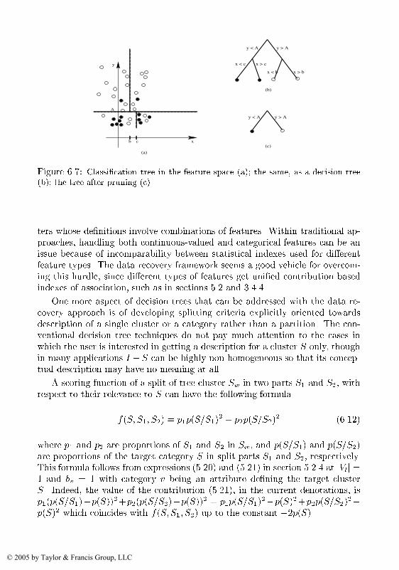
��� CONCEPTUAL DESCRIPTION OF CLUSTERS ���
A
b c x
y
y < A y > A
x < c x > c
x < b x > b
(a)
(b)
y < A y > A
(c)
Figure ���� Classi�cation tree in the feature space �a � the same as a decision tree�b � the tree after pruning �c �
ters whose denitions involve combinations of features� Within traditional approaches� handling both continuousvalued and categorical features can be anissue because of incomparability between statistical indexes used for di erentfeature types� The data recovery framework seems a good vehicle for overcoming this hurdle� since di erent types of features get unied contribution basedindexes of association� such as in sections ��� and ������
One more aspect of decision trees that can be addressed with the data recovery approach is of developing splitting criteria explicitly oriented towardsdescription of a single cluster or a category rather than a partition� The conventional decision tree techniques do not pay much attention to the cases inwhich the user is interested in getting a description for a cluster S only� thoughin many applications I � S can be highly nonhomogeneous so that its conceptual description may have no meaning at all�
A scoring function of a split of tree cluster Sw in two parts S� and S�� withrespect to their relevance to S can have the following formula
f�S� S�� S�� � p�p�S�S��� ! p�p�S�S��
� ������
where p� and p� are proportions of S� and S� in Sw� and p�S�S�� and p�S�S��are proportions of the target category S in split parts S� and S�� respectively�This formula follows from expressions ������ and ������ in section ����� at jVlj �� and bv � � with category v being an attribute dening the target clusterS� Indeed� the value of the contribution ������� in the current denotations� isp��p�S�S���p�S���!p��p�S�S���p�S��� � p�p�S�S��
��p�S��!p�p�S�S����p�S�� which coincides with f�S� S�� S�� up to the constant ��p�S��
© 2005 by Taylor & Francis Group, LLC
��� DIFFERENT CLUSTERING APPROACHES
����� Describing a cluster with production rules
Branches of a decision tree leading to terminal nodes labeled by class Sk of thepartition which is described by the tree� can be considered production rules ofthe format �if A then Sk� where A is the conjunctive predicate correspondingto an individual branch� Such a production rule states that if A is true fori � I � than i must belong in S� However� if A is not true for i� this does notnecessarily imply that i does not belong to S�
The problem of producing such production rules for a single cluster Sk�without any relevance to other clusters� has attracted considerable attentionfrom researchers� The problem ts well into the context of describing singleclusters rather than partitions�
A production rule technique produces a set of statements �if Ap then S��p � P � at which Ap is a conceptual� typically conjunctive� description of asubset in the feature space� that is� a predicate� A more precise formulation ofa production rule would be �for all x in the feature space� Ap�x� � x � S��Rectangles surrounding black circles on Figure ��� correspond to such production rules� A production rule is characterized by two numbers� �a� the support�that is the number of entities in the set I satisfying Ap� �b� the precision� theproportion of entities from S among those entities of I that satisfy Ap� In somemethods� descriptions Ap may overlap ����� ������ in others they don�t ����� ����As noted above� branches of a decision tree labeled by S can be consideredconjunctive production rules as well� however techniques generating productionrules directly are more specic� as they are focused only on S� the group ofinterest� Thus� there can be no false negatives from a production rule� onlyfalse positives�
Production rules may have rather small supports� Moreover� di erent production rules may cover di erent parts of S and leave some parts not coveredas shown on Figure ����
Production rule techniques conventionally have been developed for prediction rather than for description� A specic task of prediction of warehousetransactions has led to a set of the socalled association rule techniques comprising a di erent section of data mining ����� ����� ������ A transaction database�sentities� transactions� are described by a set of goods purchased by a customerso that each of the transactions is a set of items purchased in one go� An association rule is a production rule �if A then B� where A and B are nonoverlappingsets of goods� Presence�absence of an individual commodity is a binary feature�Thus� an association rule can be considered a production rule for binary dataso that association rule techniques can be applied to the problem of a singlecluster description by considering belongingness to S as B� A number of techniques have been developed for producing association rules �see a review in �����p���������
© 2005 by Taylor & Francis Group, LLC
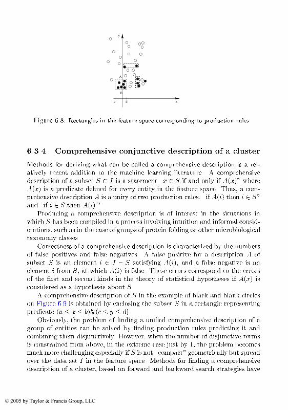
��� CONCEPTUAL DESCRIPTION OF CLUSTERS ���
A
B
c d x
y
Figure ���� Rectangles in the feature space corresponding to production rules�
����� Comprehensive conjunctive description of a cluster
Methods for deriving what can be called a comprehensive description is a relatively recent addition to the machine learning literature� A comprehensivedescription of a subset S � I is a statement �x � S if and only if A�x�� whereA�x� is a predicate dened for every entity in the feature space� Thus� a comprehensive description A is a unity of two production rules� �if A�i� then i � S�and �if i � S then A�i���Producing a comprehensive description is of interest in the situations in
which S has been compiled in a process involving intuition and informal considerations� such as in the case of groups of protein folding or other microbiologicaltaxonomy classes�Correctness of a comprehensive description is characterized by the numbers
of false positives and false negatives� A false positive for a description A ofsubset S is an element i � I � S satisfying A�i�� and a false negative is anelement i from S� at which A�i� is false� These errors correspond to the errorsof the rst and second kinds in the theory of statistical hypotheses if A�x� isconsidered as a hypothesis about S�A comprehensive description of S in the example of black and blank circles
on Figure ��� is obtained by enclosing the subset S in a rectangle representingpredicate �a � x � b�*�c � y � d��Obviously� the problem of nding a unied comprehensive description of a
group of entities can be solved by nding production rules predicting it andcombining them disjunctively� However� when the number of disjunctive termsis constrained from above� in the extreme case just by �� the problem becomesmuch more challenging especially if S is not �compact� geometrically but spreadover the data set I in the feature space� Methods for nding a comprehensivedescription of a cluster� based on forward and backward search strategies have
© 2005 by Taylor & Francis Group, LLC
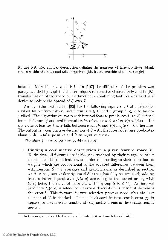
��� DIFFERENT CLUSTERING APPROACHES
x
y
g h
P
Q
Figure ���� Rectangular description de�ning the numbers of false positives �blankcircles within the box and false negatives �black dots outside of the rectangle �
been considered in ���� and ������ In ����� the di�culty of the problem waspartly avoided by applying the techniques to cohesive clusters only and in ����transformation of the space by arithmetically combining features was used as adevice to reduce the spread of S over I �
An algorithm outlined in ���� has the following input� set I of entities described by continuouslyvalued features v � V and a group S � I to be described� The algorithm operates with interval feature predicates Pf �a� b� denedfor each feature f and real interval �a� b�� of values a � x � b� Pf �a� b��x� � � ifthe value of feature f at x falls between a and b� and Pf �a� b��x� � � otherwise�The output is a conjunctive description of S with the interval feature predicatesalong with its false positive and false negative errors�
The algorithm involves two building steps�
�� Finding a conjunctive description in a given feature space V�To do this� all features are initially normalized by their ranges or othercoe�cients� Then all features are ordered according to their contributionweights which are proportional to the squared di erences between theirwithingroup S � I averages and grand means� as described in section������ A conjunctive description of S is then found by consecutively addingfeature interval predicates fv�a� b� according to the sorted order� with�a� b� being the range of feature v within group S �v � V �� An intervalpredicate fv�a� b� is added to a current description A only if it decreasesthe error�� This forward feature selection process stops after the lastelement of V is checked� Then a backward feature search strategy isapplied to decrease the number of conjunctive items in the description� ifneeded�
�In this way� correlated features are eliminated without much fuss about it�
© 2005 by Taylor & Francis Group, LLC
��� CONCEPTUAL DESCRIPTION OF CLUSTERS ���
�� Expanding the feature space V� This operation is applied if there aretoo many errors in the description A found on the rst step� It producesa new feature space by arithmetically combining original features v � Vwith those occurring in the found description A�
These two steps can be reiterated up to a prespecied number of featurecombining operations� Step � transforms and arithmetically combines the features to extend the set of potentially useful variables� Then Step � is appliedto the feature space thus enhanced� The combined variables appearing in thederived decision rule are then used in the next iteration� for combining with theoriginal variables again and again� until a prespecied number of combiningoperations� t� is reached� For example� one iteration may produce a featurev�v�� the second may add to this another feature� leading to v�v�! v�� andthe third iteration may further divide this by v�� thus producing the combinedfeature f � �v� v� ! v���v� with three combining operations�
This iterative combination process will be referred to as APPCOD �APProximate COmprehensive Description�� An APPCOD iteration can be considereda specication of the recombination step in genetic algorithms ����� The di erence is that the diversity of the original space here is maintained by using theoriginal variables at each recombination step� rather than by the presence of�bad� solutions in conventional genetic algorithms�
In this way� given a feature set V � entity set I � and class S � I � APPCODproduces a new feature set F �V �� a conjunction of the interval feature predicatesbased on F �V �� A� and its errors� the numbers of false positives FP and falsenegatives FN� Since the algorithm uses withinS ranges of variables� it ts intothe situation in which all features are quantitative� However� the algorithm canalso be applied to categorical features presented with dummy zeroone variables�just intervals �a� b� here should satisfy the condition a � b� that is� correspondto either of values� � or ��
It should be mentioned that a more conventional approach to nding a gooddescription A with mixed scale variables involves building logical predicates overcombinations of features ���� and �����
Example ����� Combined features to describe Body mass groups
Let us apply APPCOD to the Body mass data in Table ��� with the restrictionof no more than one feature combining operation� Depending on which of the groupsoverweight or normal�weight is to be described the algorithm �rst selects eitherWeight or Height� This gives a lousy description of the group with too many falsepositives� Then APPCOD combines the feature with the other one and produces thedi�erence Height � Weight and the ratio Height�Weight for both the overweight andthe normal�weight groups� The overweight group is described with these combinedfeatures with no errors whereas the normal group cannot be described distinctivelywith them� This means that the former group is somewhat more compact in thecombined feature space� The overweight group�s comprehensive description is� ���� �H�W � ���� & �� � H �W � �� with no errors�
© 2005 by Taylor & Francis Group, LLC
��� DIFFERENT CLUSTERING APPROACHES
The second inequality can be reinterpreted as stating that the di�erence Height� Weight for the other normal group is about � which �ts well into the knowncommon sense rule� �Normally the di�erence between Height �cm and Weight �kg ought to be about ���
When the number of permitted feature combining operations increases to � and thenumber of conjunctive items is limited by � the method produces the only variableH �H�W which distinctively describes either group and in fact is the inverse bodymass index used to de�ne the groups� �
�� Overall assessment
There is a great number of clustering methods that have been and are beingdeveloped� In section ���� a number of di erent clustering methods that can betreated as extensions of KMeans clustering have been presented� These methods are selected because of their great popularity� There are rather straightforward extensions of KMeans among them� such as Partitioning around medoids�in which the concept of centroid is specied to be necessarily an observed entity�and Fuzzy KMeans� in which entity memberships can be spread over severalclusters� Less straightforward extensions are represented by the regressionwiseclustering� in which centroids are regression functions� and selforganizing mapsSOM that combine the Minimum distance rule with visualization of the clusterstructure over a grid� The probabilistic mixture of distributions is a far reaching extension� falling within the statistics paradigm with a set of rather rigidrequirements such as that all features are continuousvalued and must be standardized with the zscore transformation� none of which needs to be assumedwithin the data recovery approach�Two graphtheoretic clustering methods are presented in section ���� One is
the quite popular single linkage method related to connected components andminimum spanning trees� The other is a rather new method oriented towardsnding a central dense core cluster� the method works well when such a densecore is unique�Conceptual description of clusters is covered in the last section� Three di er
ent types of conceptual description are highlighted� ��� decision tree� the mostpopular means for conceptual classication in machine learning� ��� productionrule� a device for picking up conditions leading to belongingness to a cluster�and ��� comprehensive description� which is oriented towards formulation ofnecessary and su�cient conditions of belongingness to a cluster� The problemof conceptual description of clusters has not yet found any general satisfactorysolution�
© 2005 by Taylor & Francis Group, LLC
Chapter �
General Issues
After reading through this chapter you will get a general understanding ofexisting approaches to�
�� Data preprocessing and standardization�
�� Imputation of missing data�
�� Feature selection and extraction�
�� Various approaches to determining number of clusters�
�� Validation of clusters with indexes and resampling�
and contributions of the data recovery approach to these issues�
Base words
Bootstrapping A resampling technique in which a copy of the data set iscreated by randomly selecting either rows or columns� with replacement�as many times as there are respective number of rows or columns in thedata�
Cluster validation A procedure for validating a cluster structure or clusteringalgorithm� This can be based on an internal index� or external indexor resampling� An internal index scores the degree of correspondencebetween the data and the cluster structure� An external index comparesthe cluster structure with a structure given externally� A resampling isused to see whether the cluster structure is stable with respect to datachange�
���
© 2005 by Taylor & Francis Group, LLC
��� GENERAL ISSUES
Cross�validation A resampling technique that provides for a full coverage ofthe data set� The data set is randomly divided in a number Q of equallysized parts and Q copies of the data in the �training�testing� format aregenerated by taking each of the parts as the test part in a correspondingcopy�
Dis similarity between partitions A partitiontopartition measure basedon the contingency table� All measures reviewed in this chapter can beexpressed as the weighted averages of subsettosubset measures�
Dis similarity between sets A subsettosubset measure relying on the subsets� overlap size� A popular Jaccard coe�cient relates the overlap size tothat of the union and has both advantages and shortcomings� Somewhatbetter measures should involve the ratios of the overlap size to each of thesubsets or Quetelet coe�cients�
Feature extraction A procedure for creating such �synthetic� data featuresthat maintains the most important information of a pattern in question�
Feature selection A procedure for nding such a subspace of data featuresthat retains the most important information of a pattern in question�
Index based validation Validation of a cluster structure involving either aninternal index� measuring degree of correspondence between the data andthe clusters� or an external index� measuring the correspondence betweenthe cluster structure and an externally specied partition or other externaldata�
Number of clusters An important characteristic of a cluster structure� whichdepends both on the data and the user�s objectives� There have been developed a number of criteria for determining a �right� number of clusters�both indexbased and resampling based� so far none has come up as applicable across diverse data ranges�
Resampling An approach to creating an empirical distribution of a data mining pattern or criterion by creating a number of random copies of the datatable and independently applying to them the method for computing thepattern or criterion of interest� The distribution is used for assessingvalidity of the algorithm or pattern�criterion�
© 2005 by Taylor & Francis Group, LLC
��� FEATURE SELECTION AND EXTRACTION ���
�� Feature selection and extraction
����� A review
The problem of reducing the number of features may arise in a technical contextto make a huge data set treatable computationally� In some contexts the drivingforce can be interpretation� in which the number of features involved seems agood index of clarity� the better a problem or phenomenon is understood thefewer the number of features needed to describe it� Issues of reducing the sizeof the feature space in clustering problems attract considerable interest fromresearchers ���� ����There are several dividing lines apparent in these e orts� One is to distin
guish between methods for feature selection and methods for feature extraction�The former are aimed at choosing a smaller subset from the entire set of features and the latter at producing a few �synthetic� variables from the givenones� Another divide is between situations in which clusters are prespeciedand those in which they are not� that is� between supervised and unsupervisedlearning problems�One more division arises from the way selected features are assessed� In par
ticular� under supervised learning� when a partition is prespecied� two typesof methods of feature selection or extraction are distinguished ����� wrapper and�lter� When a method for class prediction� a classier� has been selected� itsresults on di erent feature spaces can be compared with the prespecied partition and� in this way� used for selection of the best feature space� Comparisonof the classier results with the partition can be done according to di erentscoring functions� The simplest is just counting the number of errors made bythe classier on a selected feature set� the fewer errors the better� More complexmeasures use various weightings of errors�correct predictions depending on thepartition class sizes� a review of some comparison measures can be found in������ Since the interrelation between the prespecied partition and wrapperresults amount to a confusion matrix� which is a contingency table� contingencyassociation coe�cients discussed in sections ����� and ����� can be utilized� aswell as the external validation indexes in section ������ The classier serves as awrapper of di erent feature spaces� which explains the name given to this typeof evaluation methods� Wrapper methods can be used for both feature selectionand feature extraction� Results of a wrapper method are straightforward andeasy to use� however� they may depend highly on the wrapper utilized�To apply wrapper methods for feature selection in clustering� even for a
situation in which a �true� partition has been prespecied� a clustering� ratherthan prediction� method should be used as a wrapper� Such a wrapper clustering method can be referred to as a cluster maker� The closer clustering resultsare to the true partition� the better the cluster maker� Obviously� the samestrategy can be applied when the quality of a feature space is to be judged by
© 2005 by Taylor & Francis Group, LLC
��� GENERAL ISSUES
the relation of results not necessarily to a prespecied partition but some otherfeature�s��
Another class of methods constitute socalled lter methods� A lter methodselects or builds features based on a scoring function f�W � dened for everyfeature set W � V �
Probably the simplest within this class is the case of additive f�W � in whichf�W � can be represented as the sum of feature weights� f�W � �
Pv�W fv�
where fv is feature v�s weight� Under supervised learning� when a prespeciedpartition is known� feature weights can be dened according to their associationwith the partition or its classes� In particular� for a quantitative feature� itsclusterspecic weight is typically dened by the di erence between the feature�sgrand mean and within cluster mean� in general� the greater the di erence thefurther away is the cluster from the data center� thus the better the feature forseparating the cluster from the rest ����� For a categorical feature� its saliencedepends on its association to the partition� This means that contribution coefcients derived in section ��� are appropriate for the task� Sometimes� featureweights are dened within a classier computed with respect to the prespeciedpartition� as� for example� standardized coe�cients of variables in a linear discriminant function or logistic regression�
In the unsupervised situation feature saliencies can be dened according tofeature variance measured by contribution to the scatter� or entropy� or dissimilarity from other features� For example� according to a traditional approach�the feature set is rst partitioned into groups of similar features� and then a�central� feature is selected from each of the groups� Such a method will produce feature subset fNC�SC� Peg based on the partition of the Masterpieces�feature set presented in Figure ��� �b��
Sometimes a scoring function can be dened according to substantive considerations� For instance� in text mining features are key words or phrases� thenumber of occurrences of a keyword appears to be a good indicator� the mostrelevant keywords are those whose occurrence numbers are somewhere betweenthe minimum �occasional terms� and maximum �common words�� More onweighting of variables can be found in �����
If the scoring function f�W � is not additive� which is the case in wrapper methods� its optimization can be computationally challenging� To simplifycalculations� greedy methods are frequently employed� Among them the mostpopular are socalled Forward Search Selection �FSS� and Backward Search Selection �BSS� approaches� An FSS method starts with emptyW and iterativelyupdates W by adding just one� the best possible� feature at each iteration untila stopping criterion is met� A stopping criterion may involve reaching a prespecied number of features in W or a threshold to the value of f�W �� A BSSmethod starts fromW � V � the set of all features� and at each iteration removesone feature v from it� that one at which f�W � v� is optimal over v � W �
© 2005 by Taylor & Francis Group, LLC
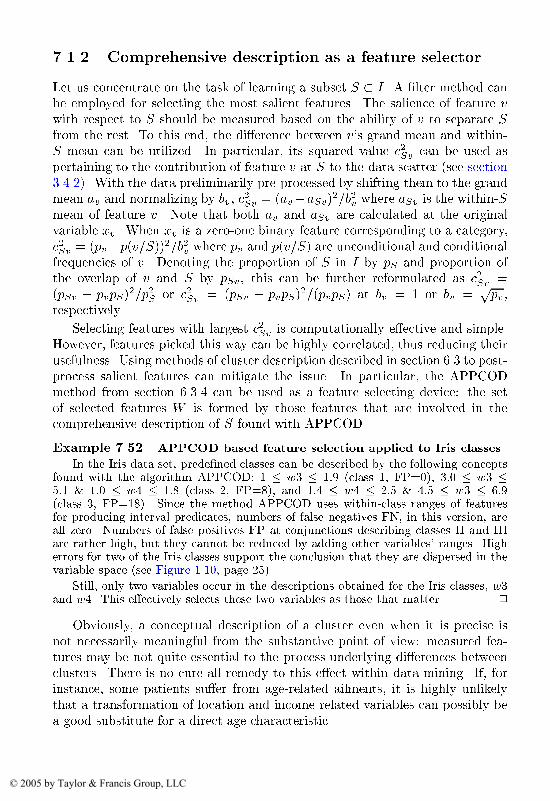
��� FEATURE SELECTION AND EXTRACTION ���
����� Comprehensive description as a feature selector
Let us concentrate on the task of learning a subset S � I � A lter method canbe employed for selecting the most salient features� The salience of feature vwith respect to S should be measured based on the ability of v to separate Sfrom the rest� To this end� the di erence between v�s grand mean and withinS mean can be utilized� In particular� its squared value c�Sv can be used aspertaining to the contribution of feature v at S to the data scatter �see section������� With the data preliminarily preprocessed by shifting them to the grandmean av and normalizing by bv� c
�Sv � �av�aSv���b�v where aSv is the withinS
mean of feature v� Note that both av and aSv are calculated at the originalvariable xv � When xv is a zeroone binary feature corresponding to a category�c�Sv � �pv�p�v�S����b�v where pv and p�v�S� are unconditional and conditionalfrequencies of v� Denoting the proportion of S in I by pS and proportion ofthe overlap of v and S by pSv � this can be further reformulated as c
�Sv �
�pSv � pvpS���p�S or c
�Sv � �pSv � pvpS�
���pvpS� at bv � � or bv �ppv�
respectively�
Selecting features with largest c�Sv is computationally e ective and simple�However� features picked this way can be highly correlated� thus reducing theirusefulness� Using methods of cluster description described in section ��� to postprocess salient features can mitigate the issue� In particular� the APPCODmethod from section ����� can be used as a feature selecting device� the setof selected features W is formed by those features that are involved in thecomprehensive description of S found with APPCOD�
Example ����� APPCOD based feature selection applied to Iris classes
In the Iris data set prede�ned classes can be described by the following conceptsfound with the algorithm APPCOD� � � w� � ��� �class � FP� �� � w� ���� & �� � w� � ��� �class � FP�� and ��� � w� � ��� & ��� � w� � ����class � FP��� � Since the method APPCOD uses within�class ranges of featuresfor producing interval predicates numbers of false negatives FN in this version areall zero� Numbers of false positives FP at conjunctions describing classes II and IIIare rather high but they cannot be reduced by adding other variables� ranges� Higherrors for two of the Iris classes support the conclusion that they are dispersed in thevariable space �see Figure ��� page �� �
Still only two variables occur in the descriptions obtained for the Iris classes w�and w�� This e�ectively selects these two variables as those that matter� �
Obviously� a conceptual description of a cluster even when it is precise isnot necessarily meaningful from the substantive point of view� measured features may be not quite essential to the process underlying di erences betweenclusters� There is no cureall remedy to this e ect within data mining� If� forinstance� some patients su er from agerelated ailments� it is highly unlikelythat a transformation of location and income related variables can possibly bea good substitute for a direct age characteristic�
© 2005 by Taylor & Francis Group, LLC
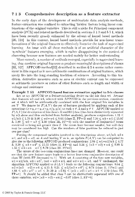
��� GENERAL ISSUES
����� Comprehensive description as a feature extractor
In the early days of the development of multivariate data analysis methods�feature extraction was conned to extracting �hidden� factors being linear combinations of the original variables� This is still a niche for Principal componentanalysis �PCA� and related methods described in sections ����� and ������ whichhave been recently grossly enhanced by the advent of kernel based methods���� ����� In this context� kernel based methods provide for nonlinear transformations of the original features to e ectively linearize the task of supervisedlearning� An issue with all these methods is of an articial character of the�synthetic� features emerging� which is rather disappointing in the context ofclustering because new features are needed mainly for better understanding�More recently� a number of methods emerged� especially in supervised learn
ing� that combine original features to produce meaningful descriptions of classes���� ����� APPCOD method���� described in section ����� seems rather convenient in this regard as it uses arithmetic combinations of original features� whichnicely ts into the longstanding tradition of sciences� According to this tradition� derivative measures such as area or electric current can be expressedas arithmetic products or ratios of other features such as length and width orvoltage and resistance�
Example ����� APPCOD based feature extraction applied to Iris classesLet us try APPCOD as a feature�extracting device on the Iris data set� Assume
that features w� and w� selected with APPCOD in the previous section constituteset A which will be arithmetically combined with the four original Iris variables inset V � We denote by F �A�V the set of features produced by applying each of �veoperations �x�y� x�y� x�y� x�y� y�x to each x � A and y � V � APPCOD applied toF �A�V for description of Iris classes II and III �class I has been distinctively separatedby w� alone and thus excluded from further analysis produces conjunctions ���� �w��w� � ��� & ��� � w� � w� � ���� �class II FP�� and ��� � w� � w� � �����& ��� � w� � w� � ��� �class III FP�� with the number of conjunctive termsrestricted to being not greater than �� The errors have become smaller but still theymay be considered too high� Can the numbers of false positives be reduced to justone per class�
Putting the compound variables involved in the descriptions above w��w� w� �w� and w� � w� as A and leaving V as is an update F �A� V can be computed togive rise to the following APPCOD produced conjunctions� ���� � w��w��w� � ����& ��� � w� � w�� � ����� �class II FP�� and ���� � �w� � w� � w� � ���� &���� � w� � w�� w� � ��� �class III FP�� �
The errors of the two�term conjunctions have not changed� However one couldsee that the new feature space leads to a better four�term conjunctive description ofclass III �with FP decreased to � � With set A consisting of the four new variablesw� � w��w� w� � w�� �w� � w� � w� and w� � w� � w� and V unchanged thealgorithm APPCOD applied to F �A�V leads to the following conjunctions� ��� �w� � �w� � w� � w� � ���� & ��� � w���w� � w�� � ��� �class II FP�� and���� � w� � w�� � w� � ���� & ����� � �w� � w� � w� � w� � ���� �class IIIFP�� � It should be added that class I can be distinctively separated with one ofthese variables w� � �w�� w� � w� � ���� �class � FP� �
© 2005 by Taylor & Francis Group, LLC
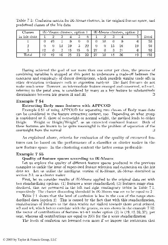
��� FEATURE SELECTION AND EXTRACTION ���
Table ���� Confusion matrix for iK�Means clusters in the original feature space andprede�ned classes of the Iris data�
Classes iK�Means clusters option � iK�Means clusters option �in Iris data � � � � � � � � � � � Total
� �� � � �� �� � � �� �� �� �� �� �� � �� �� �� � �� �
Total �� �� �� �� �� �� �� � �� �� �� ��
Having achieved the goal of not more than one error per class the process ofcombining variables is stopped at this point to underscore a trade�o� between theexactness and complexity of cluster descriptions which parallels similar trade�o�s inother description techniques such as regression analysis� The �nal features do notmake much sense� However an intermediate feature emerged and conserved w� �w�referring to the petal area is considered by many as a key feature to substantivelydiscriminate between Iris genera II and III� �
Example �����Extracting Body mass features with APPCOD
Example ���� of using APPCOD for separating two classes of Body mass datacan be considered in the feature extracting context too� Depending on what groupis considered as S those of overweight or normal weight the method leads to eitherHeight � Weight or Height�Weight� as an extracted combined feature� Both ofthese features are known to be quite meaningful in the problem of separation of theoverweight from the normal� �
As explained above� criteria for evaluation of the quality of extracted features can be based on the performance of a classier or cluster maker in thenew feature space� In the clustering context the latter seems preferable�
Example �����Quality of feature spaces according to iK Means
Let us explore the quality of di�erent feature spaces produced in the previousexamples to tackle the issue of supervised feature selection and extraction on the Irisdata set� Let us utilize the intelligent version of K�Means iK�Means described insection ��� as a cluster maker�
First let us consider results of iK�Means applied to the original data set withtwo standardizing options� �� features z�score standardized� �� features range stan�dardized that are presented in the left and right contingency tables in Table ���respectively� The cluster discarding threshold in iK�Means was set to be equal to ��
Table ��� shows that the level of confusion is less in the case of the range stan�dardized data �option � � This is caused by the fact that with this standardizationcontributions of features to the data scatter are shifted towards those petal relatedw� and w� which better correlate with the genera as was shown in the example �����the vector of contributions of features w��w� under option �� is ���� ��� ��� �� percent whereas all contributions are equal to ��� for the z�score standardization�
The levels of confusion are lessened even more if we impose the restriction that
© 2005 by Taylor & Francis Group, LLC
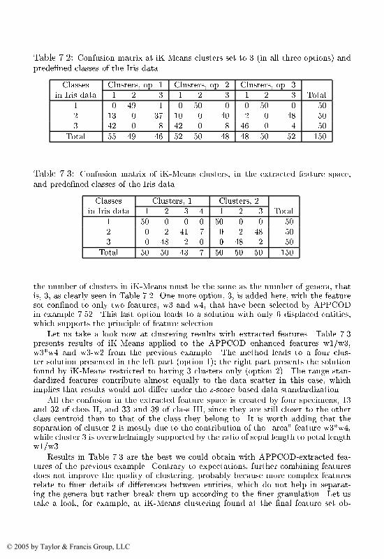
��� GENERAL ISSUES
Table ���� Confusion matrix at iK�Means clusters set to � �in all three options andprede�ned classes of the Iris data�
Classes Clusters op� � Clusters op� � Clusters op� �in Iris data � � � � � � � � � Total
� �� � � � �� �� �� � � � �� �� �� � �� � �� � �
Total �� �� �� �� � �� �� � �� ��
Table ���� Confusion matrix of iK�Means clusters in the extracted feature spaceand prede�ned classes of the Iris data�
Classes Clusters � Clusters �in Iris data � � � � � � � Total
� � � �� � �� � � �� �� �� � �� � �
Total � � �� � � � � ��
the number of clusters in iK�Means must be the same as the number of genera thatis � as clearly seen in Table ���� One more option � is added here with the featureset con�ned to only two features w� and w� that have been selected by APPCODin example ����� This last option leads to a solution with only � displaced entitieswhich supports the principle of feature selection�
Let us take a look now at clustering results with extracted features� Table ���presents results of iK�Means applied to the APPCOD enhanced features w��w�w�'w� and w��w� from the previous example� The method leads to a four clus�ter solution presented in the left part �option � � the right part presents the solutionfound by iK�Means restricted to having � clusters only �option � � The range stan�dardized features contribute almost equally to the data scatter in this case whichimplies that results would not di�er under the z�score based data standardization�
All the confusion in the extracted feature space is created by four specimens ��and �� of class II and �� and �� of class III since they are still closer to the otherclass centroid than to that of the class they belong to� It is worth adding that theseparation of cluster � is mostly due to the contribution of the �area� feature w�'w�while cluster � is overwhelmingly supported by the ratio of sepal length to petal lengthw��w��
Results in Table ��� are the best we could obtain with APPCOD�extracted fea�tures of the previous example� Contrary to expectations further combining featuresdoes not improve the quality of clustering probably because more complex featuresrelate to �ner details of di�erences between entities which do not help in separat�ing the genera but rather break them up according to the �ner granulation� Let ustake a look for example at iK�Means clustering found at the �nal feature set ob�
© 2005 by Taylor & Francis Group, LLC
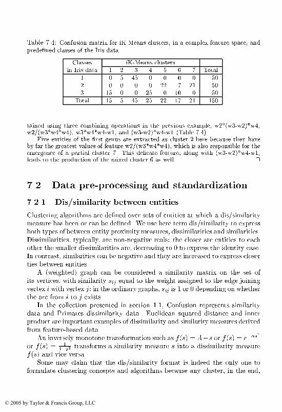
��� DATA PRE�PROCESSING AND STANDARDIZATION ���
Table ���� Confusion matrix for iK�Means clusters in a complex feature space andprede�ned classes of the Iris data�
Classes iK�Means clustersin Iris data � � � � � � � Total
� � �� �� �� � �� �� �� �� � �
Total �� � �� �� �� �� �� ��
tained using three combining operations in the previous example w�'�w��w� 'w�w���w�'w�'w� w�'w�'w��w� and �w��w� 'w��w� �Table ��� �
Five entities of the �rst genus are extracted as cluster � here because they haveby far the greatest values of feature w���w�'w�'w� which is also responsible for theemergence of a partial cluster �� This delicate feature along with �w��w� 'w��w�leads to the production of the mixed cluster � as well� �
�� Data pre�processing and standardization
����� Dis�similarity between entities
Clustering algorithms are dened over sets of entities at which a dis�similaritymeasure has been or can be dened� We use here term dis�similarity to expressboth types of between entity proximity measures� dissimilarities and similarities�Dissimilarities� typically� are nonnegative reals� the closer are entities to eachother the smaller dissimilarities are� decreasing to � to express the identity case�In contrast� similarities can be negative and they are increased to express closerties between entities�A �weighted� graph can be considered a similarity matrix on the set of
its vertices� with similarity sij equal to the weight assigned to the edge joiningvertex i with vertex j� in the ordinary graphs� sij is � or � depending on whetherthe arc from i to j exists�In the collection presented in section ���� Confusion represents similarity
data and Primates dissimilarity data� Euclidean squared distance and innerproduct are important examples of dissimilarity and similarity measures derivedfrom featurebased data�An inversely monotone transformation such as f�s� � A�s or f�s� � e��s
�
or f�s� � ���s� transforms a similarity measure s into a dissimilarity measure
f�s� and vice versa�Some may claim that the dis�similarity format is indeed the only one to
formulate clustering concepts and algorithms because any cluster� in the end�
© 2005 by Taylor & Francis Group, LLC
��� GENERAL ISSUES
is determined in terms of dis�similarities between entities� In fact� features canbe useful as well because�
�� Clustering methods such as KMeans may employ the specicity of thevector space format to explicitly formulate the concept of cluster�s prototype or centroid as a feature based entity�
�� Features are involved in cluster interpretation�
�� The vector space format can be by far more e ective computationallywhen the number of features is relatively small� Think of the di erencebetween NM input numbers in the vector space and N� or N��� inputnumbers in the dis�similarity format when N is large andM small� If� forinstance� there are ������ entities and ��� features� there will be about onemillion numbers in the former case and about a hundred million numbersin the latter case� the di erence which can be crucial with contemporarypersonal computers�
The idea of conversion of dis�similarity based data into the feature spaceformat motivated a lot of research in the socalled multidimensional scaling� thediscipline oriented towards embedding given dis�similarity data into a vectorspace in such a way that the betweenentity distances in the space would approximate the prespecied dis�similarities� An issue with this approach is thatthe found space has no intrinsic interpretational support� In our view� this canbe overcome with another idea gaining more and more popularity that� givena dis�similarity data table� a number of entities should be preselected as reference points serving as coordinate axes so that each entity can be representedby the vector of its distances to the reference points�
Complex data such as chemical compound formulas� timeseries of stockprices� biomolecular sequences� images� etc� can be used for automaticallydiscovering patterns such as motives in sequences or edges in images that can beused then for feature generation� This implies that the preprocessing issues arenot necessarily purely computational ones but can involve specic data miningtechniques including clustering� These topics remain beyond the scope of thistext� Relevant materials can be found in ���� �sequences and temporal data������� �images�� ���� �data bases and warehouses�� ���� �spatial data��
����� Preprocessing feature based data
The only preprocessing issue raised in this book concerns categorical and mixedscale features�
Traditionally� mixed scale feature data are treated by transforming theminto a dissimilarity matrix D � �dij�� where i� j � I are entities� according to
© 2005 by Taylor & Francis Group, LLC
��� DATA PRE�PROCESSING AND STANDARDIZATION ���
the formula�
dpij �Xf�F
wf jxif � yjf jp !Xv�V
wv jxiv � yjv jp �����
where p is the socalled Minkowsky�s power� typically� taken as p � � or p � ��F � V are respectively sets of quantitative features and qualitative categories�wf and wv are userdened weight coe�cients for features f � F and categoriesv � V � and xiv are ��� values �� at entities i falling in the category v and � atthe rest�� Similarity measures are dened analogously by summing up weightedsimilarities between i and j at individual features and categories�
Some may say that formula ����� does not much di er� at p � �� from theEuclidean distance squared used in this text� and in fact� is even more generalbecause it involves weights wf and wv � Yes� indeed� It is exactly the extent ofgenerality which is fought o with the help of the data recovery approach� Thecommon opinion is that the weight coe�cients are to come from the user� �Thechoice of measure will be guided largely by the type of variables being used andthe intuition of the investigator� ������ p� ���� The current author argues thisbecause in most cases the user has no clue regarding to the weights in formula������ According to this book�s approach the weights are supposed to comefrom data� not the user� This is provided by the recommended preprocessingand standardization technique described in section ���� With data xiv and xifstandardized into yiv and yif the weights in distance ����� become wv � ��b
pv�
v � F � V � with bv being scaling coe�cients derived from the data�To substantiate this recipe� let us bring forward the following�
�� Introducing dummy variables for categories extends the concept of quantitative scale as that admitting the operation of averaging to qualitative categories� averaging dummies leads to conditional and unconditional probabilities �frequencies�� which is exactly the machinery utilized in methodsspecically oriented for analysis of categorical data�
�� Rescaling of categories is an e ective instrument to maintain appropriatecontributions of categories to the data scatter and� in this way� provideconsistency to the process of simultaneously analyzing quantitative andqualitative data�
�� Summary contributions of dummy variables to the explained part of thedata scatter appear to be in line with intuitive criteria proposed withinthe qualitative data framework such as the category utility function andPearson chisquare contingency coe�cient applied in conceptual clustering and decision tree building� This property brings a rather di erentlight to the contingency coe�cients for cross classications� It appears�
© 2005 by Taylor & Francis Group, LLC
��� GENERAL ISSUES
they must be considered on par with the correlation ratio for quantitative variables and� moreover� get unexpectedly transformed� one into theother� depending on the data normalization option accepted�
�� The data recovery framework helps in addressing one of the major issues ofdata analysis� warranting that data preprocessed into the dis�similarityformat get no additional structures imposed by the preprocessing� Statements proven in sections ��� and ��� allow us to claim that there are criteria and methods that should lead to compatible results in both featurebased and dis�similarity data� More explicitly� if a dissimilarity measureis equal �or similar� to the squared Euclidean distance squared betweenrows of a vector space matrix� or a similarity measure is the rowtorowinner product� then compatible criteria and local search heuristics arethose detailed in section ������
����� Data standardization
Data standardization is performed featurewise and�or entitywise to make features and�or entities comparable� The issue of comparability of features can beillustrated with the Market towns data set in Table ���� obviously the scale offeature Population is a thousand times greater than of any other feature in thetable� thus di erences in this feature will dominate the dis�similarities betweenentities� This contradicts the principle of equal importance of features� whichunderlies cluster analysis as well as many other methods of multivariate dataanalysis� The principle states that in the situation when no explicit weights canbe assigned to features they should equally contribute to the result� This principle is underlined by the assumption that the user controls the process of dataanalysis by structuring the phenomenon under consideration into meaningfulaspects and then assigning features to the aspects� The relative importance ofan aspect is re�ected by the number of features assigned to it� In this way� theequivalence of features is translated into the relative importance of the aspects�The practical implementation of the equivalence principle is usually done
via� rst� standardization of the variables and� second� balancing contributionsof standardized features into entitytoentity distances ����� ���� A similar approach has been advised in this text� The only di erence is that the distances� inour context� are not a primary but derivative tool� it is the data recovery models and criteria which are primary� The distances are generated by the squareerror criteria of these models� the balance of contributions can be maintainedin the criteria as well� and data scatter decompositions provide a feedback tocompare contributions�Shifting the origin and changing the scale with formula yiv � �xiv � av��bv
������ is the main device for feature standardization� More radical proposalsinclude further data transformation along lines that are akin to the singular
© 2005 by Taylor & Francis Group, LLC
��� DATA PRE�PROCESSING AND STANDARDIZATION ���
value decomposition of the data matrix and� thus� should be considered partof data analysis rather than data preprocessing� It should be pointed out thatthere are cases in which the scale may be left unchanged� that is� bv taken tobe unity� such is the case of binary features or� more generally� the situationsin which every feature presents a ranking within the same rank scale� say from� to ��
However� proposals for setting values of av and bv may highly di er� In particular� the value of the shift coe�cient av has been suggested in the literatureto be equal to any of the following�
�a�� ��
�a�� minimum� mini�I xiv �
�a�� maximum� maxi�I xiv �
�a�� midrange� �maxi�I xiv !mini�I xiv����
�a�� grand mean� the average of xiv over all i � I �
�a�� median�
Similarly� it has been suggested that the value of the scale coe�cient bv betaken as any of the following�
�b�� range rv or halfrange rv�� with rv � maxi�I xiv �mini�I xiv ��b�� standard deviation sv �
pPi�I �xiv � "xv���N� where N� is either N
or N � �� the latter value due to probabilistic considerations of mathematicalstatistics�
�b�� grand mean "xv � the average of xiv over all i � I �
Among scaling coe�cients� the most popular option is the standard deviation� probably because it is inherited from methods of mathematical statisticsassuming the normal distribution of data at which the joint action of options�a�� and �b��� referred to as zscoring� is the natural choice� I also subscribed tothis option� in the context of nonprobabilistic data analysis� as an explicationof the principle of equal importance of features� with bv � sv � contributions ofall features to the data scatter are equal to each other ����� However� this recommendation is overly simplistic� The value of standard deviation depends ontwo factors� the feature scale size and the shape of its distribution� Obviously�the distribution shape is important in clustering� a multimodal distributionmay be evidence of the multicluster structure� However� normalizing featureswith the standard deviation forces bi and moremodal features to shrink to asmaller weight than they should �see also section ������� The other two options�normalizing by the range or average� catch the size factor only� while leavingthe distribution aside and� thus� should be preferred in clustering� A popularoption rescales data in such a way that all values fall within interval ���� ���which is achieved with av being midrange �a�� and bv range �b��� Anotheroption pulls all data into the interval ������ by using �a�� and �b��� to be able�formally� to apply operations and interpretations referring to proportions andfrequencies�
© 2005 by Taylor & Francis Group, LLC
��� GENERAL ISSUES
In ���� a set of computational experiments have been performed with a number of distancebased clustering methods and various standardization options�The methods included a range of agglomerative procedures from the single linkage to Ward agorithms� The data generated consisted of a small number� ��� ofpoints of small� � to �� dimensions� concentrated in a number of well separatedclusters� supplemented with errors being either �i� normally distributed noiseadded to data entries� or �ii� two additional� randomly generated� features� or�iii� �� outlier points added to the set� Overall� the normalization by rangeappeared to unanimously provide for the best recovery of the underlying clusterstructure among other normalization options� �the traditional zscore formulawas not especially e ective�� ������ p� ����� This concurs with the advicefollowing from the analysis of feature contributions to the Pythagorean decomposition in section ����Subtracted shift values av play no role in the distance ������ but they do
work when using the inner product as a similarity measure and� more importantly� in cluster centroids� In this regard� the recommended option �a�� for avbeing the grand mean has obvious advantages� With this� the cluster centroidsexpress the di erences between the feature withincluster averages and grandmeans � these di erences accentuate each cluster�s specics� The di erences areindispensable in interpreting clusters and� moreover� they are behind the entiresystem of clusterfeature contributions to the data scatter� The appropriatenessof using grand means as the shift coe�cients is underscored by the properties ofthese contributions relating them to classical ideas of statistics� the correlationratio� Quetelet indexes� and the Pearson chisquare association coe�cient� Theworking of the Anomalous pattern method and iKMeans clustering is basedon that� too�
�� Similarity on subsets and partitions
Subsets and partitions play an important role in clustering on both sides of thedata pipeline� the input and output�On the input side� a binary category can be equivalently represented� up
to the corresponding metadata� by the subset of entities falling under thecategory� Thus� binary data tables can be considered sets of subsets� Binaryfeatures constitute a most important specic data format to which many otherdata formats can be preprocessed� Examples include�
�� Sets of keywords� expertdriven or found automatically� for documents�
�� Sets of neighboring representatives�
�� Genome contents�
�� Network neighborhoods�
© 2005 by Taylor & Francis Group, LLC
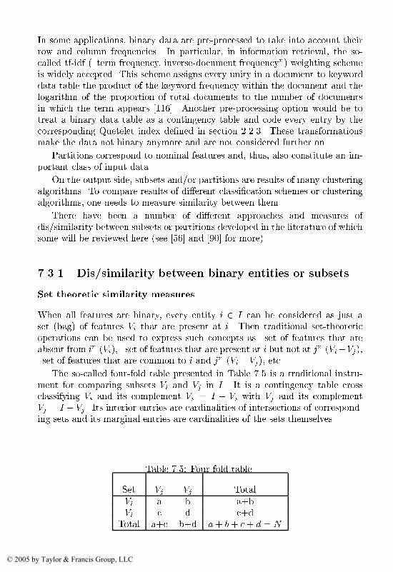
��� SIMILARITY ON SUBSETS AND PARTITIONS ���
In some applications� binary data are preprocessed to take into account theirrow and column frequencies� In particular� in information retrieval� the socalled tfidf ��term frequency� inversedocument frequency�� weighting schemeis widely accepted� This scheme assigns every unity in a documenttokeyworddata table the product of the keyword frequency within the document and thelogarithm of the proportion of total documents to the number of documentsin which the term appears ������ Another preprocessing option would be totreat a binary data table as a contingency table and code every entry by thecorresponding Quetelet index dened in section ������ These transformationsmake the data not binary anymore and are not considered further on�
Partitions correspond to nominal features and� thus� also constitute an important class of input data�
On the output side� subsets and�or partitions are results of many clusteringalgorithms� To compare results of di erent classication schemes or clusteringalgorithms� one needs to measure similarity between them�
There have been a number of di erent approaches and measures ofdis�similarity between subsets or partitions developed in the literature of whichsome will be reviewed here �see ���� and ���� for more��
����� Dis�similarity between binary entities or subsets
Set theoretic similarity measures
When all features are binary� every entity i � I can be considered as just aset �bag� of features Vi that are present at i� Then traditional settheoreticoperations can be used to express such concepts as �set of features that areabsent from i� � "Vi�� �set of features that are present at i but not at j� �Vi�Vj���set of features that are common to i and j� �Vi � Vj�� etc�The socalled fourfold table presented in Table ��� is a traditional instru
ment for comparing subsets Vi and Vj in I � It is a contingency table crossclassifying Vi and its complement "Vi � I � Vi with Vj and its complement"Vj � I � Vj � Its interior entries are cardinalities of intersections of corresponding sets and its marginal entries are cardinalities of the sets themselves�
Table ���� Fourfold table�
Set Vj "Vj TotalVi a b a!b"Vi c d c!d
Total a!c b!d a! b! c! d � N
© 2005 by Taylor & Francis Group, LLC
��� GENERAL ISSUES
Probably the simplest similarity measure is the size of the overlap�
ij � jVi � Vj j � a� �����
However� this measure fails to relate the size of the overlap to the set sizesand thus does not allow us to judge whether the overlap comprises the bulk orjust tip of the sets� The distance between sets dened as�
h�i� j� � jVi � Vj j � jVi � Vj j � jVij! jVj j � �jVi � Vj j � b! c� �����
is somewhat better� It is � when Vi � Vj � but its maximum� jVi � Vj j� stilldepends on the set sizes� Returning to binary rows xi and xj of the data tablecorresponding to entities i and j� it is easy to see that distance h�i� j� indeedequals the squared Euclidean� and indeed cityblock� distance between xi andxj �
h�i� j� �Xv�V
�xiv � xjv�� �
Xv�V
jxiv � xjv j�
The latter equation follows from the fact that �x�x��� � jx�x�j for any binaryx and x�� Measure h�i� j� ����� is referred to as Hamming distance between thebinary vectors�The relative distance h�i� j��N is known as the mismatch coe�cient between
sets�
m�i� j� � h�i� j��N � �b! c��N �����
Its complement to unity� the socalled match coe�cient�
s�i� j� � �N � h�i� j���N � �a! d��N� �����
is popular as well�Index s�i� j� is always between � and �� It is � when Vi � Vj and it is �
when Vi and Vj are complementary parts of I �An issue with s�i� j� as a similarity measure is that it depends on the size
N of I which may be irrelevant� especially in comparing two �little things inthe big world� such as two text documents among thousands of others�The socalled Jaccard coe�cient �����
J�i� j� �jVi � Vj jjVi � Vj j �
a
a! b! c� �����
does not depend on N � �It is sometimes referred to as the Tanimoto coe�cient��This measure takes into account only features that are present at either i or jor both and handles them in such a way that the value of J does not dependon the total feature set� It ranges between � and �� and it is � when Vi � Vj
© 2005 by Taylor & Francis Group, LLC
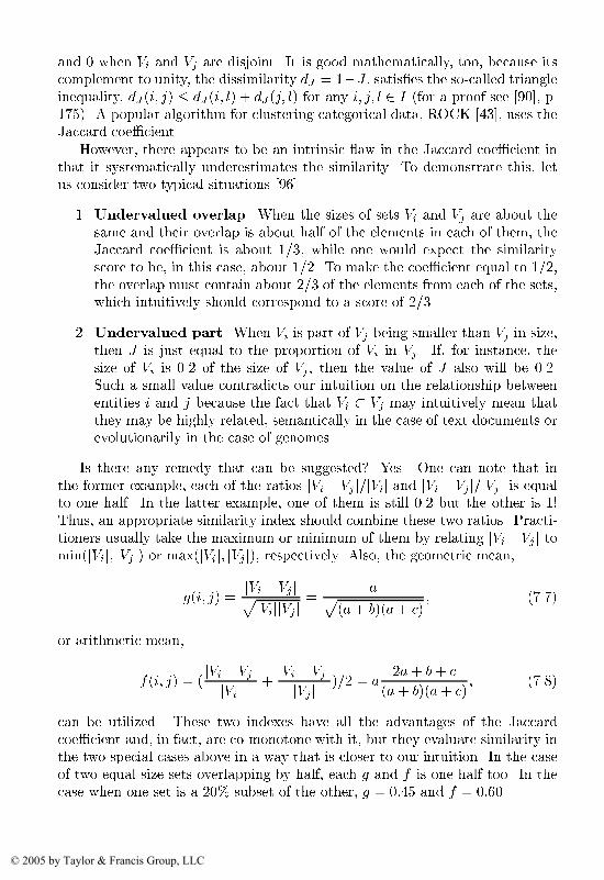
��� SIMILARITY ON SUBSETS AND PARTITIONS ���
and � when Vi and Vj are disjoint� It is good mathematically� too� because itscomplement to unity� the dissimilarity dJ � ��J � satises the socalled triangleinequality� dJ�i� j� � dJ�i� l� ! dJ�j� l� for any i� j� l � I �for a proof see ����� p������ A popular algorithm for clustering categorical data� ROCK ����� uses theJaccard coe�cient�However� there appears to be an intrinsic �aw in the Jaccard coe�cient in
that it systematically underestimates the similarity� To demonstrate this� letus consider two typical situations �����
�� Undervalued overlap� When the sizes of sets Vi and Vj are about thesame and their overlap is about half of the elements in each of them� theJaccard coe�cient is about ���� while one would expect the similarityscore to be� in this case� about ���� To make the coe�cient equal to ����the overlap must contain about ��� of the elements from each of the sets�which intuitively should correspond to a score of ����
�� Undervalued part� When Vi is part of Vj being smaller than Vj in size�then J is just equal to the proportion of Vi in Vj � If� for instance� thesize of Vi is ��� of the size of Vj � then the value of J also will be ����Such a small value contradicts our intuition on the relationship betweenentities i and j because the fact that Vi � Vj may intuitively mean thatthey may be highly related� semantically in the case of text documents orevolutionarily in the case of genomes�
Is there any remedy that can be suggested� Yes� One can note that inthe former example� each of the ratios jVi � Vj j�jVij and jVi � Vj j�jVj j is equalto one half� In the latter example� one of them is still ��� but the other is �#Thus� an appropriate similarity index should combine these two ratios� Practitioners usually take the maximum or minimum of them by relating jVi � Vj j tomin�jVij� jVj j� or max�jVij� jVj j�� respectively� Also� the geometric mean�
g�i� j� �jVi � Vj jpjVijjVj j �
ap�a! b��a! c�
� �����
or arithmetic mean�
f�i� j� � �jVi � Vj jjVij !
jVi � Vj jjVj j ��� � a
�a! b! c
�a! b��a! c�� �����
can be utilized� These two indexes have all the advantages of the Jaccardcoe�cient and� in fact� are comonotone with it� but they evaluate similarity inthe two special cases above in a way that is closer to our intuition� In the caseof two equal size sets overlapping by half� each g and f is one half too� In thecase when one set is a �� subset of the other� g � ���� and f � �����
© 2005 by Taylor & Francis Group, LLC
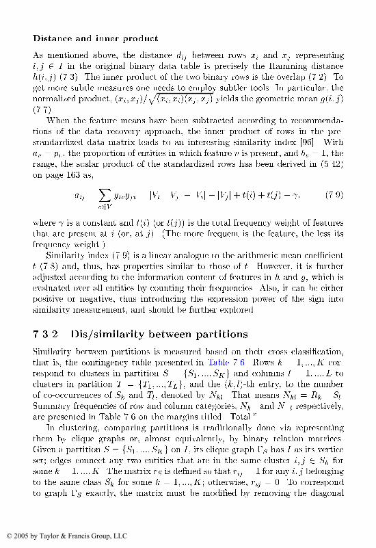
��� GENERAL ISSUES
Distance and inner product
As mentioned above� the distance dij between rows xi and xj representingi� j � I in the original binary data table is precisely the Hamming distanceh�i� j� ������ The inner product of the two binary rows is the overlap ������ Toget more subtle measures one needs to employ subtler tools� In particular� thenormalized product� �xi� xj��
p�xi� xi��xj � xj� yields the geometric mean g�i� j�
������When the feature means have been subtracted according to recommenda
tions of the data recovery approach� the inner product of rows in the prestandardized data matrix leads to an interesting similarity index ����� Withav � pv� the proportion of entities in which feature v is present� and bv � �� therange� the scalar product of the standardized rows has been derived in ������on page ��� as�
aij �Xv�V
yivyjv � jVi � Vj j � jVij � jVj j! t�i� ! t�j� ! �� �����
where � is a constant and t�i� �or t�j�� is the total frequency weight of featuresthat are present at i �or� at j�� �The more frequent is the feature� the less itsfrequency weight��Similarity index ����� is a linear analogue to the arithmetic mean coe�cient
t ����� and� thus� has properties similar to those of t� However� it is furtheradjusted according to the information content of features in h and g� which isevaluated over all entities by counting their frequencies� Also� it can be eitherpositive or negative� thus introducing the expression power of the sign intosimilarity measurement� and should be further explored�
����� Dis�similarity between partitions
Similarity between partitions is measured based on their cross classication�that is� the contingency table presented in Table ���� Rows k � �� ����K correspond to clusters in partition S � fS�� ���� SKg and columns l � �� ���� L toclusters in partition T � fT�� ���� TLg� and the �k� l�th entry� to the numberof cooccurrences of Sk and Tl� denoted by Nkl� That means Nkl � Rk � Sl�Summary frequencies of row and column categories� Nk� and N�l respectively�are presented in Table ��� on the margins titled �Total��In clustering� comparing partitions is traditionally done via representing
them by clique graphs or� almost equivalently� by binary relation matrices�Given a partition S � fS�� ���� SKg on I � its clique graph +S has I as its verticeset� edges connect any two entities that are in the same cluster i� j � Sk forsome k � �� ����K� The matrix rS is dened so that rij � � for any i� j belongingto the same class Sk for some k � �� ����K� otherwise� rij � �� To correspondto graph +S exactly� the matrix must be modied by removing the diagonal
© 2005 by Taylor & Francis Group, LLC
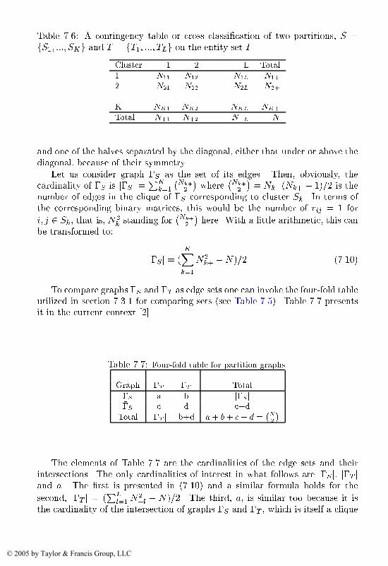
��� SIMILARITY ON SUBSETS AND PARTITIONS ���
Table ���� A contingency table or cross classication of two partitions� S �fS�� ���� SKg and T � fT�� ���� TLg on the entity set I �
Cluster � � ��� L Total
� N�� N�� ��� N�L N��
� N�� N�� ��� N�L N��
��� ��� ��� ���� ��� ���K NK� NK� ��� NKL NK�
Total N�� N�� ��� N�L N
and one of the halves separated by the diagonal� either that under or above thediagonal� because of their symmetry�Let us consider graph +S as the set of its edges� Then� obviously� the
cardinality of +S is j+S j �PK
k��
�Nk�
�
�where
�Nk�
�
�� Nk��Nk� � ���� is the
number of edges in the clique of +S corresponding to cluster Sk� In terms ofthe corresponding binary matrices� this would be the number of rij � � for
i� j � Sk� that is� N�k standing for
�Nk�
�
�here� With a little arithmetic� this can
be transformed to�
j+S j � �KXk��
N�k� �N��� ������
To compare graphs +S and +T as edge sets one can invoke the fourfold tableutilized in section ����� for comparing sets �see Table ����� Table ��� presentsit in the current context ����
Table ���� Four�fold table for partition graphs�
Graph (T �(T Total
(S a b j(S j�(S c d c�d
Total j(T j b�d a � b � c � d ��N�
�
The elements of Table ��� are the cardinalities of the edge sets and theirintersections� The only cardinalities of interest in what follows are j+S j� j+T jand a� The rst is presented in ������ and a similar formula holds for the
second� j+T j � �PL
l��N��l � N���� The third� a� is similar too because it is
the cardinality of the intersection of graphs +S and +T � which is itself a clique
© 2005 by Taylor & Francis Group, LLC
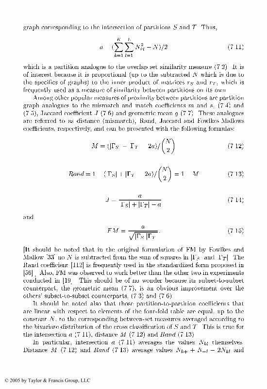
��� GENERAL ISSUES
graph corresponding to the intersection of partitions S and T � Thus�
a � �
KXk��
LXl��
N�kl �N��� ������
which is a partition analogue to the overlap set similarity measure ������ It isof interest because it is proportional �up to the subtracted N which is due tothe specics of graphs� to the inner product of matrices rS and rT � which isfrequently used as a measure of similarity between partitions on its own�Among other popular measures of proximity between partitions are partition
graph analogues to the mismatch and match coe�cients m and s� ����� and������ Jaccard coe�cient J ����� and geometric mean g ������ These analoguesare referred to as distance �mismatch�� Rand� Jaccard and FowlkesMallowscoe�cients� respectively� and can be presented with the following formulas�
M � �j+S j! j+T j � �a���N
�
�������
Rand � �� �j+S j! j+T j � �a���N
�
�� ��M ������
J �a
j+S j! j+T j � a������
and
FM �apj+S jj+T j � ������
�It should be noted that in the original formulation of FM by Fowlkes andMallow ���� no N is subtracted from the sum of squares in j+S j and j+T j� TheRand coe�cient ����� is frequently used in the standardized form proposed in������ Also� FM was observed to work better than the other two in experimentsconducted in ����� This should be of no wonder because its subsettosubsetcounterpart� the geometric mean ������ is an obvious improvement over theothers� subsettosubset counterparts� ����� and ������It should be noted also that those partitiontopartition coe�cients that
are linear with respect to elements of the fourfold table are equal� up to theconstant N � to the corresponding betweenset measures averaged according tothe bivariate distribution of the cross classication of S and T � This is true forthe intersection a ������� distance M ������ and Rand �������In particular� intersection a ������ averages the values Nkl themselves�
Distance M ������ and Rand ������ average values Nk� ! N�l � �Nkl and
© 2005 by Taylor & Francis Group, LLC
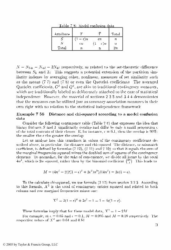
��� SIMILARITY ON SUBSETS AND PARTITIONS ���
Table ���� Model confusion data�
Attribute T �T Total
S �� � � n �n n�S �n �� � � n n
Total n n �n
N � Nk� � N�l ! �Nkl respectively� as related to the settheoretic di erencebetween Sk and Tl� This suggests a potential extension of the partition similarity indexes by averaging other� nonlinear� measures of set similarity suchas the means ����� and ����� or even the Quetelet coe�cients� The averagedQuetelet coe�cients� G� and Q�� are akin to traditional contingency measures�which are traditionally labeled as deliberately attached to the case of statisticalindependence� However� the material of sections ����� and ����� demonstratesthat the measures can be utilized just as summary association measures in theirown right with no relation to the statistical independence framework�
Example ����� Distance and chi squared according to a model confusiondata
Consider the following contingency table �Table ��� that expresses the idea thatbinary features S and T signi�cantly overlap and di�er by only a small proportion �of the total contents of their classes� If for instance � � �� then the overlap is ���the smaller the � the greater the overlap�
Let us analyze how this translates in values of the contingency coe�cients de�scribed above in particular the distance and chi�squared� The distance or mismatchcoe�cient is de�ned by formulas ����� ����� and ��� so that it equals the sum ofthe marginal frequencies squared minus the doubled sum of squares of the contingencyelements� To normalize for the sake of convenience we divide all items by the total�n� which is �n squared rather than by the binomial coe�cient
��n�
�� This leads to
M � ��n� � ����� � � � � ��� n� ���n� � ���� � � �
To the calculate chi�squared we use formula ����� from section ������ Accordingto this formula X� is the total of contingency entries squared and related to bothcolumn and row marginal frequencies minus one�
X� � ���� � � � ��� � � � � � ����� � �
These formulas imply that for these model data X� � �� �M �
For example at � � �� and � � �� M � ��� and M � ��� respectively� Therespective values of X� are ��� and ����
�
© 2005 by Taylor & Francis Group, LLC
��� GENERAL ISSUES
Matching�based similarity versus Quetelet association
We can distinguish between two types of subsettosubset and respectivepartitiontopartition association measures�
M� matching between subsets�partitions measured by their overlap a in ������������ and ������� and
C� conditional probability and Quetelet indexes such as ������ and ������ and�������
Considered as they are� in terms of cooccurrences� these two types areso di erent that� to the author�s knowledge� they have never been consideredsimultaneously� There is an opinion that� in the subsettosubset setting� theformer type applies to measuring similarity between entities whereas the lattertype to measuring association between features�
However� there exists a framework� that of data recovery models for entitytoentity similarity matrices� in which these two types represent the same measure of correlation applied in two slightly di erent settings� In this framework�each partition S � fS�� ���� SKg of the entity set I � or a nominal variable whosecategories correspond to classes Sk �k � �� ����K�� can be represented by a similarity matrix s � �sij� between i� j � I where sij � � for i and j from di erentclasses and a positive real when i and j are from the same class� Consider twodenitions�
M� sij � � if i� j � Sk for some k � �� ����K�
C� sij � ��Nk if i� j � Sk for some k � �� ����K where Nk is the number ofentities in Sk�
The assumption is that all similarities within S are the same� in the case M� orinversely proportional to the class size so that the larger the class the smallerthe similarity� in the case C� The latter re�ects the convention that the morefrequent is a phenomenon the less information value in it�
Matrix s � �sij� corresponding to a partition S has dimension N N � Itsaverage "s is "s � G�S� � ��Pk p
�k� Gini index� in the case M� or "s � ��N � in
the case C�
Let now S and T be two partitions on I � Corresponding similarity matricess � �sij� and t � �tij�� as well as their centered versions s� "s and t� "t� can beconsidered N N vectors� Then the inner product of these vectors� in the caseM� is equal to
PKk��
PLl��N
�kl featured in equation ������ whereas the inner
product of their centered versions in the case C is the Pearson chisquared�This shows that the two types of partitiontopartition measures can be relatedto the two types of entitytoentity similarities� in the data recovery framework�
© 2005 by Taylor & Francis Group, LLC
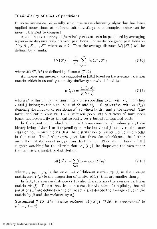
��� SIMILARITY ON SUBSETS AND PARTITIONS ���
Dissimilarity of a set of partitions
In some situations� especially when the same clustering algorithm has beenapplied many times at di erent initial settings or subsamples� there can bemany partitions to compare�A good manytomany dis�similarity measure can be produced by averaging
a pairwise dis�similarity between partitions� Let us denote given partitions onI by S�� S������ Sm where m � �� Then the average distance M�fStg� will bedened by formula�
M�fStg� � �
m�
mXu�w��
M�Su� Sw� ������
where M�Su� Sw� is dened by formula �������An interesting measure was suggested in ����� based on the average partition
matrix which is an entitytoentity similarity matrix dened by
��i� j� �
Pmt�� s
tij
m��i� j�������
where st is the binary relation matrix corresponding to St with stij � � when
i and j belong to the same class of St and stij � �� otherwise� with m��i� j�denoting the number of partitions St at which both i and j are present� Thelatter denotation concerns the case when �some of� partitions St have beenfound not necessarily at the entire entity set I but at its sampled parts�In the situation in which all m partitions coincide� all values ��i� j� are
binary being either � or � depending on whether i and j belong to the sameclass or not� which means that the distribution of values ��i� j� is bimodalin this case� The further away partitions from the coincidence� the furtheraway the distribution of ��i� j� from the bimodal� Thus� the authors of �����suggest watching for the distribution of ��i� j�� its shape and the area underthe empirical cumulative distribution�
A�fStg� �LXl��
��l � �l���F ��l� ������
where ��� ��� ���� �L is the sorted set of di erent entries ��i� j� in the averagematrix and F ��� is the proportion of entries ��i� j� that are smaller than ��In fact� the average distance ������ also characterizes the average partition
matrix ��i� j�� To see that� let us assume� for the sake of simplicity� that allpartitions St are dened on the entire set I and denote the average value in thematrix by "� and the variance by ���
Statement ���� The average distance M�fStg� ���� is proportional to"���� "��� ���
© 2005 by Taylor & Francis Group, LLC
��� GENERAL ISSUES
Proof� According to denition� M�fStg� � Pmu�w��
Pi�j�I �s
uij � swij�
��m��
This can be rewritten as M�fStg� � Pi�j�I
Pmu�w���s
uij ! swij � �suijswij��m��
Applying the operations to individual items we obtain M�fStg� �Pi�j�I �
Pmw�� ��i� j��m!
Pmu�� ��i� j��m� ���i� j���i� j�� � �Pi�j�I ���i� j��
��i� j���� The proof of the statement follows then from the denition of thevariance of the matrix� q�e�d�As proven in statement ����� given a probability of smaller than the average
values� the variance of a variable reaches its maximum when the variable isbinary� The value "� in this case can be assigned the meaning of being sucha probability� Then the formula in statement ����� shows that the averagedistanceM� in fact� measures the di erence between the maximum and observedvalues of the variance of the average partition matrix� Either this di erence orthe variance itself can be used as an index of similarity between the observeddistribution of values ��i� j� and the ideal case at which all of them coincide�
�� Dealing with missing data
����� Imputation as part of preprocessing
Some data entries can be missing because of various reasons such as di�cultiesin obtaining data� or because of inaccuracy in data collecting or maintaining�or because of deciencies in data producing devices� There are two approachesto dealing with missing data����Within a method� missing data are treated within a specially modied
method for data analysis� This approach is popular with such techniques asregression analysis� but not with clustering����Before a method� imputation of missing entries is conducted as part of
data preprocessing before any more specic analyses� Researchers do recognizethat patterns of missings may relate to the data contents� in gene expressionanalyses� weak gene expression is more likely to go unnoticed� and in incomesurveys� respondents are likely to leave sensitive questions unanswered� Still�most research is being done under the assumption that missings emerge atrandom entries� In the remainder of this section� we refer to this approach only�Among the methods of imputation of incomplete data� one can distinguish
the following three approaches�
�� Conditional mean� in which every missing entry is substituted by a predicted value such as the variable�s mean or the value predicted by a regression function or decision tree ���� ��� �����
�� Maximum likelihood based methods� in which missings are imputed according to an estimated data density function ���� ����
© 2005 by Taylor & Francis Group, LLC
��� DEALING WITH MISSING DATA ���
�� Leastsquares approximation� in which the data are approximated with alowrank data matrix ���� ��� ����
Let us brie�y discuss them in turn�
����� Conditional mean
Arguably the most popular method of imputation� at least among practitioners�is the substitution of a missing entry by the corresponding variable�s mean�which will be referred to as the Mean algorithm� More subtle approaches useregression based imputation in which a regressionpredicted value is imputed���� ���� Decision trees are used for handling missing categorical data in ������The Mean algorithm has been combined with nearestneighbor based techniquesin ������Two common features of the conditional mean approaches are� ��� miss
ing entries are dealt with sequentially� onebyone� and ��� most of them relyon a limited number of variables� The other approaches handle all missingssimultaneously by taking advantage of using all the available data entries�
����� Maximum likelihood
The maximum likelihood approach relies on a parametric model of data generation� typically� the multivariate Gaussian mixture model� The maximumlikelihood method is applied for both tting the model and imputation of themissing data� The most popular is the socalled expectationmaximization �EM�algorithm ����� which exploits the popular idea of alternating optimization tomaximize the maximum likelihood criterion as described in section ������ Thepopularity of the maximum likelihood approach is based on the fact that it isgrounded on a precise statistical model� However� methods within this approachmay involve unsubstantiated hypotheses and be computationally intensive�
����� Leastsquares approximation
This is a nonparametric approach based on approximation of the available datawith a lowrank bilinear factorial model akin to the principal component analysis model ������Methods within this approach� typically� work sequentially by producing
one factor at a time to minimize the sum of squared di erences between theavailable data entries and those reconstructed via the lowrank model� Twoways to implement this approach can be distinguished�
�� Iterative least squares �ILS�� Fit a lowrank approximate data model����� by using nonmissing entries only and then interpolate the missingvalues with values found according to the model ���� ����
© 2005 by Taylor & Francis Group, LLC
��� GENERAL ISSUES
�� Iterative majorized least squares �IMLS�� Start by lling in all missing entries with some value such as zero� then iteratively approximate thuscompleted data by updating the imputed values with those implied by alowrank SVD based approximation �����
These can be combined with nearestneigbor based techniques as follows�take a row that contains a missing entry as the target entity xi� nd its Knearest neighbors in X � and form a matrix Xi consisting of the target entityand its neighbors� Then apply an imputation algorithm to the matrix Xi�imputing missing entries at the target entity only� Repeat this until all missingentries are lled in� Then output the thus completed data matrix�A globallocal approach proposed in ����� involves two stages� First stage�
Use a global imputation technique to ll in all missings in the original matrixX so that entitytoentity distances can be calculated with no concessions tothe presence of missing values� Let us denote the resulting matrix X�� Secondstage� Apply a nearestneighbor based technique to ll in the missings in Xagain� but� this time� based on distances computed with the completed datamatrix X�� This globallocal approach involving IMLS on both of the stages� inthe beginning with m � � and in the end with m � �� is referred to as algorithmINI in ������ In experiments reported in ������ nearestneighbor based leastsquares imputation algorithms give similar results outperforming other leastsquares algorithms including the Mean and nearestneighborMean imputation�When the proportion of random missings grows to �� and� moreover� �� �INI becomes the only winner ������Overall� the subject is in early stages of development� Potential mechanisms
of missings are not well dened yet�
�� Validity and reliability
����� Index based validation
After applying a clustering algorithm� the user would like to know whether theresults indeed re�ect an innate property of the data or they are just an artifactgenerated by the algorithm� In other words� the user wants to know whetherthe cluster structure found is valid or not� It is not a di�cult question whenthere is a probabilistic mechanism for data generation� which is known to theuser� Unfortunately� this is not the typical case in cluster analysis� Typically�the data come from a source that cannot be modelled this way if it can be atall� There is one more cause of uncertainty here� the user�s wish to have anaggregate representation of the data� at a level of resolution� which cannot bestraightforwardly formalized and� moreover� depends on the task at hand�There are two types of indexes used to quantify the validity� internal and
external�
© 2005 by Taylor & Francis Group, LLC
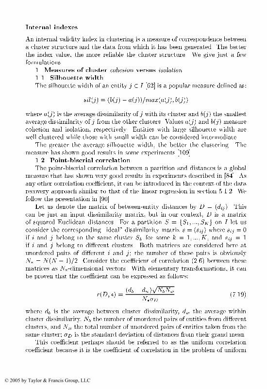
��� VALIDITY AND RELIABILITY ���
Internal indexes
An internal validity index in clustering is a measure of correspondence betweena cluster structure and the data from which it has been generated� The betterthe index value� the more reliable the cluster structure� We give just a fewformulations�
�� Measures of cluster cohesion versus isolation���� Silhouette width�The silhouette width of an entity j � I ���� is a popular measure dened as�
sil�j� � �b�j�� a�j���max�a�j�� b�j��
where a�j� is the average dissimilarity of j with its cluster and b�j� the smallestaverage dissimilarity of j from the other clusters� Values a�j� and b�j� measurecohesion and isolation� respectively� Entities with large silhouette width arewell clustered while those with small width can be considered intermediate�The greater the average silhouette width� the better the clustering� The
measure has shown good results in some experiments ���������� Point�biserial correlation�The pointbiserial correlation between a partition and distances is a global
measure that has shown very good results in experiments described in ����� Asany other correlation coe�cient� it can be introduced in the context of the datarecovery approach similar to that of the linear regression in section ������ Wefollow the presentation in �����Let us denote the matrix of betweenentity distances by D � �dij�� This
can be just an input dissimilarity matrix� but in our context� D is a matrixof squared Euclidean distances� For a partition S � fS�� ���� SKg on I let usconsider the corresponding �ideal� dissimilarity matrix s � �sij� where sij � �if i and j belong to the same cluster Sk for some k � �� ����K� and sij � �if i and j belong to di erent clusters� Both matrices are considered here atunordered pairs of di erent i and j� the number of these pairs is obviouslyN� � N�N � ����� Consider the coe�cient of correlation ����� between thesematrices as N�dimensional vectors� With elementary transformations� it canbe proven that the coe�cient can be expressed as follows�
r�D� s� ��db � dw�
pNbNw
N� D������
where db is the average between cluster dissimilarity� dw the average withincluster dissimilarity� Nb the number of unordered pairs of entities from di erentclusters� and Nw the total number of unordered pairs of entities taken from thesame cluster� D is the standard deviation of distances from their grand mean�This coe�cient perhaps should be referred to as the uniform correlation
coe�cient because it is the coe�cient of correlation in the problem of uniform
© 2005 by Taylor & Francis Group, LLC
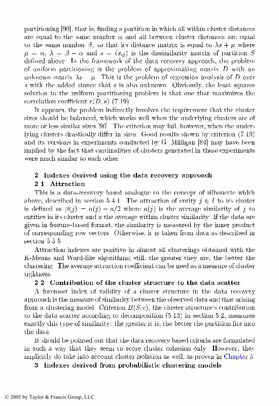
��� GENERAL ISSUES
partitioning ����� that is� nding a partition in which all within cluster distancesare equal to the same number � and all between cluster distances are equalto the same number �� so that its distance matrix is equal to s ! � where� � �� � � � � and s � �sij� is the dissimilarity matrix of partition Sdened above� In the framework of the data recovery approach� the problemof uniform partitioning is the problem of approximating matrix D with anunknown matrix s ! �� This is the problem of regression analysis of D overs with the added stance that s is also unknown� Obviously� the least squaressolution to the uniform partitioning problem is that one that maximizes thecorrelation coe�cient r�D� s� �������
It appears� the problem indirectly involves the requirement that the clustersizes should be balanced� which works well when the underlying clusters are ofmore or less similar sizes ����� The criterion may fail� however� when the underlying clusters drastically di er in sizes� Good results shown by criterion ������and its versions in experiments conducted by G� Milligan ���� may have beenimplied by the fact that cardinalities of clusters generated in these experimentswere much similar to each other�
�� Indexes derived using the data recovery approach�
���� Attraction�
This is a datarecovery based analogue to the concept of silhouette widthabove� described in section ������ The attraction of entity j � I to its clusteris dened as ��j� � a�j� � a�� where a�j� is the average similarity of j toentities in its cluster and a the average within cluster similarity� If the data aregiven in featurebased format� the similarity is measured by the inner productof corresponding row vectors� Otherwise� it is taken from data as described insection ������
Attraction indexes are positive in almost all clusterings obtained with theKMeans and Wardlike algorithms� still� the greater they are� the better theclustering� The average attraction coe�cient can be used as a measure of clustertightness�
���� Contribution of the cluster structure to the data scatter�
A foremost index of validity of a cluster structure in the data recoveryapproach is the measure of similarity between the observed data and that arisingfrom a clustering model� Criterion B�S� c�� the cluster structure�s contributionto the data scatter according to decomposition ������ in section ���� measuresexactly this type of similarity� the greater it is� the better the partition ts intothe data�
It should be pointed out that the data recovery based criteria are formulatedin such a way that they seem to score cluster cohesion only� However� theyimplicitly do take into account cluster isolation as well� as proven in Chapter ��
�� Indexes derived from probabilistic clustering models�
© 2005 by Taylor & Francis Group, LLC
��� VALIDITY AND RELIABILITY ���
A number of indexes have been suggested based on probabilistic models ofcluster structure� for a review� see ��� ���� Results of using these indexes highlydepend on the accepted model which� typically� the user has no possibility ofverifying�
Use of internal indexes to estimate the number of clusters
The issue of how to determine the number of clusters in KMeans and otherpartitional algorithms has attracted a great deal of attention in the literature�As explained in section ������ this issue is not always meaningful� However� thisdoes not mean that a review of the many attempts should be glossed over�On the rst glance� any validity measure� such as the average silhouette
width and uniform correlation explained above� can be used for selecting thenumber of clusters� just do clustering for a range of values of K and selectthat one which makes the measure maximum �or minimum if the better tcorresponds to its decrease��This idea was explored by many authors with respect to the withincluster
variance�WK � the value of W �S� c� at the found Kcluster partition� The indexas is obviously cannot be used because it monotonely decreases when K grows�the greater is the number of clusters� the better t� But its change� the rst�or even second� di erence
�WK �WK����T�
where T is the data scatter� can be considered a good signal� the number ofclusters should stop rising when this di erence becomes small� Hartigan ���� iscredited with formally shaping a similar idea� take the index�
hK � �WK�WK�� � ���N �K � ���and one by one increase K starting from �� stop calculations when hK becomesless than ��� An index by Calinski and Harabasz�
cK � ��T �WK���K � �����WK��N �K���
associated with Fisher distribution in statistics� showed a good performance insome experiments �����There are measures that compare WK with its expected value under a uni
form distribution� In particular� Krzanowski and Lai ���� showed that theexpected value of WK is proportional to K
���M where M is the dimension ofthe space� They used ratio�
K��MWK �
and its di erences to derive the best number of clusters� Similar indexes havebeen proposed in the socalled Gapstatistic ����� and Jumpstatistic ������
© 2005 by Taylor & Francis Group, LLC
��� GENERAL ISSUES
The latter seems especially suitable� calculate the average �distortion� of anaxis associated with tting K centroids to data with the KMeans algorithm�wK �WK�M whereM is the number of features andWK the value of KMeanssquare error criterion at a partition found with KMeans� and calculate �jumps�
jK � w�M��K � w
�M��K�� � With w � � and w� � T�M where T is the data
scatter� jumps can be dened for all reasonable values of K � �� �� ���� Themaximum jump corresponds to the right number of clusters� This is supportedwith a mathematical derivation stating that if the data can be considered astandard sample from a mixture of Gaussian distributions and distances between centroids are great enough� then the maximum jump would indeed occurat K equal to the number of Gaussian components in the mixture ������Reviews of these and other indexes of the best number of clusters can be
found in ����� ������ ������Experiments conducted by authors of ����� and others show that none of
them can be considered a universal criterion�In fact� the straightforward option does not necessarily work even for the av
erage silhouette width and the uniform correlation� In particular� ����� reportsthat somewhat better results could be obtained by using the average silhouettewidth indirectly� for determining that no further splits of clusters are needed�the smaller the average silhouette width within a split cluster� the more likelyit should not be split at all�There is no universal criterion because� apart from obvious cases such as
clearly seen di erences between rock and water� light and dark� horse and birchtree� clusters are not only in the data but also in the mind of the user� Thegranularity of the user�s vision and betweencluster boundaries� when no naturalboundaries can be seen� should be left to the user� This can be formalized byintroduction of relevant �external� criteria�
External indexes
The socalled external indexes compare a clustering found in data with anotherclustering either given by an expert or following from a knowledge domainor found by another clustering algorithm� Typically clusterings are sets orpartitions of the entity set I � Thus� the external indexes are those described insections ����� and ����
����� Resampling for validation and selection
Resampling is a procedure oriented at testing and improving reliability of databased estimators and rules with respect to changes in data� Basically� it produces an empirical distribution of clustering results and related indexes to seethe extent of dispersion of these with regard to data changes� This type ofanalysis has become feasible with the development of computer hardware and
© 2005 by Taylor & Francis Group, LLC

��� VALIDITY AND RELIABILITY ���
is in its infancy as a discipline� After having read through a number of recentpublications involving resampling and done some computational experiments�the author can propose the following systematic of resampling in clustering�Resampling involves the following steps�
A� Generation of a number of data sets� copies� related to the data underconsideration�
B� Running an accepted algorithm �such as regression� classication tree� orclustering� independently at each of the copies�
C� Evaluating results�
D� Aggregating�
Let us describe these steps in greater detail bearing in mind that the dataset under analysis has the standard entitytofeature format�
A Generation of copies can be done by either subsampling or splitting orperturbing the data set�
A� Subsampling� a proportion �� � � � � � � is specied and �Nentities are selected randomly without replacement in a subsample�the copy data is constituted by the rows corresponding to selectedentities�
A� Splitting� set I is randomly split in two parts of prespecied sizes�the training and testing parts� This can be done as is� by generatinga copy with a train�testing split� or via the socalled cross�validationat which the entity set is randomly split in a prespecied numberof parts Q of approximately equal size� and Q copies are createdsimultaneously� A copy is created by considering one of the Q partsas the testing set� and its complement as the training set� Typically�Q is taken as either �� � or ��� However� the case when Q is equal tothe number of entities is also popular� it is called leave�one�out crossvalidation �����
A� Perturbing� the size of a copy here is the same as in the original dataset but the entries are perturbed by�
A��� Bootstrapping� In this process� the data set is considered as thatconsisting of N rows� Uniform random sampling with replacement is applied N times to randomly pick up N row indexes�which are not necessarily di erent because of the replacements�A copy set is created then by combining the N selected rowsinto a data table� Obviously� some rows may be left out of thecreated data table since some rows may occur there two or more
© 2005 by Taylor & Francis Group, LLC
��� GENERAL ISSUES
times� It is not di�cult to estimate the probability of a row notbeing selected� At each action of picking out a row� the probability of a row not being selected is �� ��N � which implies thatthe approximate proportion of rows never selected in the sampling process is ��� ��N�N � ��e � ���� of the total numberof entities� That means that any bootstrap copy on average includes only about ���� of the entities� some of them severaltimes� A similar process can be applied to columns of the datamatrix �����
A��� Adding noise� In this process� a random real number is added toeach entry� The added number is typically generated from thenormal distribution with zero mean and a relatively small variance� In ���� a combination of bootstrapping and adding noiseis described� For a KMeans found cluster structure �S� c�� letus calculate the residuals eik in the data recovery model �������A bootstrapping experiment is then dened by randomly sampling with replacement among the residuals eiv and putting thesampled values in equations ������ to calculate the bootstrappeddata�
B Running an algorithm on a copy is done the same way as on the originaldata set except for that if the copy is obtained by splitting� the algorithmis run over its training part only�
C Evaluating results depends on the copy type� If copies are obtainedby subsampling or perturbing� the results on copies are compared to theresults found with the original data set� If copies are obtained by splitting�the training part based results are evaluated on the test part� Let usdescribe this in more detail for each of the copy types�
C� Subsample case� The cluster structure found from a subsample iscompared with the cluster structure on the same subsample resultingfrom the application of the algorithm to the original data set� Thecomparison can be done with any index such as Rand �discussedin section ������ or chisquare contingency coe�cients �discussed insection ������� For instance� in ���� the evaluation is done according to the averaged overlap index ������� in ����� relative distancebetween �sample� and �real� centroids is computed� This concernssituations in which subsample results do not depend on the subsample size� which is not so sometimes� For instance� if the tted modelinvolves a feature interval �like in APPCOD based descriptions�� theinterval�s length on an �N subsample will be� on average� � timesthe interval�s length on the original data� Then the interval must bestretched out in the proportion ��� �����
© 2005 by Taylor & Francis Group, LLC
��� VALIDITY AND RELIABILITY ���
C� Split case� The evaluation of a model tted to the training data israther easy when the model is that of prediction or description as inthe case of the regression or classication tree� In these� the trainingpart tted model is applied as is to the testing part and the errorscore of the prediction�description in the testing part is calculated�When the tted model is a cluster structure such as produced by KMeans� its evaluation in the testing part is not straightforward andcan be done di erently� For instance� in ���� the following method�Clest� is proposed� First� apply KMeans to the testing parts anew�Then build a prediction model� such as a classication tree� on thetraining part and apply it to the testing part to predict� for eachtesting part entity� what cluster it should belong to� This also can bedone by using the minimum distance rule applied to the testing partsat the training part based centroids ����� In this way� two partitionsare found on the testing part� that predicted from the training partand that found anew� The evaluation then is done by comparingthese two partitions� the closer the better �see examples in section������� An original use of the leaveoneout model for measuringsimilarity between entities is described in ����� the authors use theminimum rather than average correlation over pairwise correlationswith one column removed� this also cleans the outlier e ects�
C� Perturbation case� The evaluation is especially simple when thedata have been perturbed by adding noise� because the entities remain the same� Thus� the evaluation can be done by comparing thecluster structure found with the original data and cluster structurefound at the perturbed data� In the case of partitions� any of the indexes of section ����� would t� In ���� evaluation is done by testingthe perturbed data partition against the original centroids� the erroris proportional to the number of cases in which the minimum distancerule assigns an entity to a di erent cluster� In the case of bootstrap�evaluation can be done by comparing those parts of the two clusterstructures� which relate to that aspect of data that was not changedby the sampling� In particular� Felsenstein ���� suggested bootstrapping columns �features� rather than entities in building hierarchicalclusters and more generally phylogenetic trees� Evaluation of resultsis performed by comparing entity clusters found on the perturbeddata with those found on the original data� the greater the numberof common clusters� the better�
D Aggregating results� This can be done in various ways such as thefollowing�
D� Combining evaluations� Typically� this is just averaging the eval
© 2005 by Taylor & Francis Group, LLC
��� GENERAL ISSUES
uations for each individual copy� The averaged score can be considered as a test result for the algorithm� In this way� one can selectthe best performing algorithm among those tested� This can also beapplied to selection of parameters� such as the number of clusters�with the same algorithm ����� ����� The results on perturbed copiescan be used to score condence in various elements of the clusterstructure found at the original data set� For instance� in ����� eachof the hierarchic clusters is accompanied by the proportion of copieson which the same algorithm produced the same cluster� the greaterthe proportion� the greater the condence�
D� Averaging models� Models found with di erent copies can beaveraged if they are of the same format� The averaging is not necessarily done by merely averaging numerical values� For instance� aset of hierarchical clustering structures can be averaged in a structure that holds only those clusters that are found in a majority ofthe set structures ����� In ����� centroids found at subsamples areconsidered a data set which is clustered on its own to produce theaveraged centroids�
D� Combining models� When models have di erent formats� as inthe case of decision trees that may have di erent splits over di erentfeatures at di erent copies� the models can be combined to form a�committee� in such a way that it is their predictions rather thanthemselves that are averaged� Such is the procedure referred to asbagging in �����
����� Model selection with resampling
Since a quality score such as the number of misclassied entities or the contribution to the data scatter may be di erent over di erent samples� resamplingcan be used not only for testing� but for learning� too� Of a set of algorithmsone is selected at which an accepted quality score coe�cient is optimized� Thisis called model selection� Examples of model selection can be found in Efronand Tibshirani ���� p� ������ �selection of decision tree sizes�� Salzberg ������p� ������ �averaging probabilities obtained with splitsamplebased decisiontrees� and the following subsections�
Determining the number of clusters with K�Means
This subject has been treated in a number of publications ���� ��� ���� ����� Letus describe a method proposed in ������ This method exploits the properties ofthe average partition matrix ��i� j� �i� j � I� and the empirical distribution ofits entries described above on page ����
© 2005 by Taylor & Francis Group, LLC
��� VALIDITY AND RELIABILITY ���
Let us specify a number K� perform KMeans on many random subsamplesfrom the entity set I � dene the average partition matrix ��i� j� based on partitions found and the area under its cumulative distribution� A�K�� as denedby formula ������� After having done this for K � �� �� ���Kmax� B�K
�
� is dened as the maximum of A�K�� K � �� ����K
�
� Then the relative area increaseis expressed as %�K� � �A�K ! �� � B�K���B�K�� K � �� �� ���� At K � ��%�K� is dened as %��� � A���� Based on a number of simulation studies� theauthors of ����� claim that the maximum of this index is indicative of the truenumber of clusters�
Model selection for cluster description
To learn a comprehensive description of a subset S � I � we apply a resamplingprocess that can be considered a model of generalization in a learning device�According to this model� the learning process is organized in two stages� Atthe rst stage� the learning device is presented with di erent samples of thedata� in which Sentities are indicated� Based on these� the learning devicedevelops a set of combined features that are most e ective for separating Sfrom the rest� At the second stage� the device is again presented with randomsupervised data samples� Now samples are used not for feature generation butrather for building an aggregate conjunctive description in terms of featuresgenerated at the rst stage�These stages can be characterized in brief as follows �����
�� Extracting features� At this stage� a number of random samples fromthe pair �I� S� is generated� and the APPCOD algorithm of comprehensivedescription is applied to each of them� The best of these descriptions isselected to proceed� The quality of a description is evaluated by its erroron the entire data set�
To extend an � sample based description to the whole data set� eachfeature interval predicate is extended by stretching its interval out by thereverse coe�cient ���� This generally breaks the property of APPCODproduced predicates to cover the entire withinS ranges of the featuresand thus restores the ability to have both false positive and false negativeerrors�
To measure the error� one may use either the conventional total numberof errors FP ! FN or the more subtle criterion E � �FP�jI � Sj !��� ��FN�jSj of the weighted summary proportion of errors� Changingweight coe�cient � allows one to take into account the relative importance of false positives versus false negatives� If S is a cancer type� falsenegatives should be avoided �� is to be close to ��� false positives are ofan issue when S are loyal customers �� is to be close to ��� Otherwise�
© 2005 by Taylor & Francis Group, LLC
��� GENERAL ISSUES
keep � � ���� Relative� not absolute� values of the errors appear in E toaddress the situations in which S is signicantly smaller than I � S�
The features occurring in the best comprehensive description are considered e ective for learning set S in I and added to the feature set�
�� Selecting descriptions� At this stage� a number of independent samples from �I� S� is generated again and an APPCOD produced descriptionis found at each of them� However� this time the APPCOD is used as afeature selector� not extractor� Only features present after the rst stage�not their combinations� are used in producing feature interval predicates�Then sample descriptions are aggregated according to a version of themajority rule� only features occurring at the majority of sample descriptions are selected� Their intervals are determined by averaging the leftand right boundaries of intervals involved in the sample feature intervalpredicates�
The algorithm can be tuned up with two principal parameters� the maximum number of items permitted in a conjunctive description� l� and the numberof arithmetic operations admitted in a combined feature� f � This proceeds in aloop over f and l� starting with a value of � for each and doing the loop over lwithin the loop over f � Based on our experimentation� these were set f�� andthe limits of l set from l � ��f � �� ! � to l � �f by default� For any givenpair� l and f � the generalization process applies a number of times �three� bydefault� and the best result is picked up and stored �����
Example ����� Generalization with resampling at Body mass data�Applied to the Body mass data in Table ��� this method produces either the body
mass index Weight��Height'Height or the less expressive variables Weight�Heightand Height � Weight depending on numbers of random samples at each step of thegeneralization process described above� When both numbers are small the less ex�pressive variables tend to appear� When the number of samples at the Aggregatingstep increases the method produces the body mass index� This tendency is muchless expressed when the number of samplings increases at the Generalization step�Curiously these tendencies practically do not depend on the sample size� �
Example ����� Binary data� Republicans and democrats at the US con gressional voting
Let us describe results of applying the APPCOD based model selection methodon the data set of ���� United States Congressional Voting Records from #���$ whichcontains records of sixteen yes�no votings by ��� democrats and ��� republicans�It appears the set of republicans can be described by just one predicate p��esa��admitting �� FP and FN ����� of total error� Here p� and esa are abbreviationsof issues �physician�fee�freeze� and �export�administration�act�south�africa� and �codes yes� and no��
This means that all republicans and only �� democrats voted consistently onboth issues either both yes or both no which cannot be described that short without
© 2005 by Taylor & Francis Group, LLC
�� OVERALL ASSESSMENT ���
the operation of division� Another issue� the method describes each individual classasymmetrically which allows us to check which of the classes republican or democratis more coherent� Because of the asymmetry in APPCOD one can safely claim thatthe class whose description has the minimum error is more coherent� Descriptionsof democrats found at various subsamples always had ��� times more errors thandescriptions of republicans which �ts very well into the popular images of theseparties #��$� �
� Overall assessment
The chapter reviews a number of issues of current interest in clustering as partof data mining�First� the issue of nding a relevant feature space is considered� There are
two approaches here� feature selection and feature transformation �extraction��Automatic transformation of the feature space is a major problem in data mining which is yet to be properly addressed� Arithmetically combining featureswithin the context of a decision rule maker� specically� the comprehensivedescription algorithm� can be of value in attacking the problem�Second� issues and approaches in data preprocessing and standardization�
including dealing with missing data� are discussed � advantages of the datarecovery approach are pointed out�Third� issues of cluster validity including those of determining the �right�
number of clusters� are addressed in terms of� �a� internal and external indexesand �b� data resampling�Internal indexes show the correspondence between data and clusters derived
from them� Obviously� the best source of such indexes are the data recoverycriteria and related coe�cients� Unfortunately� none of the indexes proposed sofar can be considered a universal tool because of both the diversity of data andcluster structures and the di erent levels of granulation required in di erentproblems�External indexes show correspondence between datadriven clusters and
those known from external considerations� We provide a description of suchindexes in section ��� in such a way that correspondences between settosetand partitiontopartition indexes are established� as well as relations betweenstructural and association indexes�Data resampling as a tool for model testing and selection is a relatively new
addition� A systematic review of the approaches is given based on the most recent publications� A data resampling based model for learning a comprehensivedescription of a cluster is discussed�
© 2005 by Taylor & Francis Group, LLC
Conclusion� Data Recovery
Approach in Clustering
Traditionally clusters are built based on similarity� A found cluster of similarentities may be used as a whole to generalize and predict� This order of actionis reversed in the data recovery approach� A property of similarity clusters�the possibility to aggregate data of individual entities into data of clusters� istaken here as the dening attribute� According to the data recovery approach�entities are brought together not because they are similar but because they canbe used to better recover the data they have been built from� Is it not just anew name for old wine� Indeed� the closer the entities to each other the moreeach of them resembles the cluster�s prole�
Yet the shift of the focus brings forward an important di erence� In thedata recovery approach� the concept of similarity loses its foundation statusand becomes a derivative of the criterion of recovery� In conventional clustering�the emphasis is on presenting the user with a number of options for measuringsimilarity� the greater the choice the better� There is nothing wrong with thisidea when the substantive area is well understood� But everything is wrong withthis when the knowledge of the substantive area is poor� No user is capableof reasonably choosing a similarity measure in such a situation� A similaritymeasure should come from the data mining side� This is the case in which adata recovery approach can provide sound recommendations for the similaritymeasurement and� moreover� for the data preprocessing needed to balanceitems constituting the data recovery criterion�
The heart of the data recovery clustering framework is Pythagorean decomposition of the data scatter into two items� that explained by the cluster structure and that unexplained� the square error� The items are further decomposedin the contributions of individual entity�feature pairs or larger substructures�Some developments that follow from this�
�� Pre�processing�
�a� The data scatter expresses the scattering of entities around the originof the feature space� which thus must be put into a central� or normal�
���
© 2005 by Taylor & Francis Group, LLC
��� CLUSTERING FOR DATA MINING
position among the entity points �this position is taken to be thegrand mean��
�b� The data scatter is the sum of feature contributions that are proportional to their variances thus re�ecting the distribution shapes� thisallows for tuning feature normalization options by separating scaleand shape related parts�
�c� The strategy of binary coding of the qualitative categories in orderto simultaneously process them together with quantitative features�which cannot be justied in conventional frameworks� is supportedin this framework with the following�
i� Binary features appear to be the ultimate form of quantitativefeatures� those maximally contributing to the data scatter�
ii� The explained parts of category contributions sum up to association contingency coe�cients that already have been heavilyinvolved in data analysis and statistics� though from a very different perspective�
iii� The association coe�cients are related to the data normalization options� which can be utilized to facilitate the user�s choiceamong the latter� this can be done now from either end� theprocess� input or output� or both�
iv� The equivalent entitytoentity similarity measure which hasemerged in the data recovery context is akin to best heuristicsimilarity measures but goes even further by taking into accountthe information weights of categories�
�� Clustering�
�a� Data recovery models for both KMeans and Ward clustering extend the Principal Component Analysis �PCA� model to the casesin which scoring vectors are to be compulsory binary or tertiary�respectively� This analogy should not be missed because the PCAitself is conventionally considered but a heuristic method for extracting the maximum variance from the data� which is not quite correct�In fact� the PCA can be justied by using a data recovery model� asshown in section ������ and then extended to clustering�
�b� KMeans is the method of alternating minimization applied to thesquare error criterion�
�c� Agglomerative and divisiveWard clustering involve somewhat �dual�decompositions of the data scatter� That for divisive clustering is anatural one� treating the scatter�s unexplained part as a whole andfurther decomposing the explained part into items related to the
© 2005 by Taylor & Francis Group, LLC
CONCLUSION ���
contributions of individual clusters and features� In contrast� thedecomposition for agglomerative clustering hides the structure of theexplained part� which probably can explain why no specic tools forthe interpretation of cluster hierarchies have been proposed before�
�d� By exploiting the additive structure of the data recovery models inthe manner following that of the PCA method� onebyone clusteringmethods are proposed to allow for e ective computational schemesas well as greater �exibility in a controlled environment� In particular� the intelligent version of KMeans� iKMeans� can be used forincomplete clustering with removal of devious or� in contrast� overlynormal items� if needed�
�e� Local search algorithms presented lead to provably tight clusters� the fact expressed with the attraction coe�cient� a theorybasedanalogue to popular criteria such as the silhouette width coe�cient�
�f� The approach is extended to contingency and �ow data by takinginto account the property that each entry is a part of the whole�The entries are naturally standardized into the Quetelet coe�cients�the corresponding data scatter appears to be equal to the chisquaredcontingency coe�cient�
�g� The inner product can be used as an equivalent device in the correspondingly changed criteria� thus leading to similarity measures andclustering criteria � some of those are quite popular and some arenew� still being similar to those in use�
�� Interpretation aids�
�a� The models provide for using the traditional cluster centroids asindicators of cluster tendencies� Also� more emphasis is put on thestandardized� not original� values thus relating them to the overallnorms �averages��
�b� Inner products of individual entities and centroids� not distances between them that are used conventionally� express entity contributionsto clusters� This relates to the choice of a cluster representative aswell� not by the distance but by the inner product�
�c� The decomposition of the data scatter over clusters and features intable ScaD provides for comparative analysis of the relative contributions of all elements of the cluster structure� especially with Queteletcoe�cients �table QScaD�� to reveal the greatest of them�
�d� APPCOD� a method for conceptual description of individual clustersbased on the table ScaD� can serve as a supplementary or complementary tool to classical decision trees as interpretation and descriptionaids�
© 2005 by Taylor & Francis Group, LLC
��� CLUSTERING FOR DATA MINING
�e� In hierarchical classication� the conventional decomposition of thedata scatter over splits and clusters has been supplemented withsimilar decompositions of feature variances� covariances and individual entries� these may be used as aids in the interpretation of thetendencies of hierarchical clusters�
�f� The decomposition of the data scatter over an upper cluster hierarchycan now be visualized with the concept of the boxchart� extendingthe conventional piecharts�
Much room remains for further developments and extensions of the datarecovery approach�First� data specics� such as those that we considered here only for the cases
of mixed and contingency data tables� should be taken into account� Consider� for instance� digitized image data� Here entities are pixels organized ina grid� Conventionally� image data are compressed and processed with techniques exploiting their spatial character with such constructions as quadtreesand wavelets� which are unrelated in the current thinking� The data recoverymodel with upper cluster hierarchies� used here for developing divisive Wardlike clustering� in fact can be considered as an extension of both quadtrees andwavelets� This may potentially lead to methods of image processing while simultaneously compressing them� Another promising area is applying the datarecovery approach to analysis of temporal or spatiotemporal data� An advantage of modeling data with a cluster model is that the temporal trajectory of acluster centroid can be modeled as a specic� say exponential� function of time�Gene expression data contain measurements of several properties made over thesame gene array spots� they should be considered another promising direction�Second� the models themselves can be much improved beyond the simplest
formats employed in the book� These models� in fact� require any data entry to be equal to a corresponding entry in a centroid or a combination ofcentroids� This can be extended to include �gray� memberships� transformedfeature spaces� and logically described clusters� The least squares criterion canbe changed for criteria that are less sensitive to data variation� The least modulicriterion is a most obvious alternative� Possibilities of probabilistic modellingshould not be discarded either� In the current setting� the Pythagorean decompositions much resemble those used for the analysis of variance of a singlevariable over various groupings� Related probabilistic models� included in moststatistics texts� seem� however� overly rigid and restrictive� Hopefully� clusteranalysis may provide a ground for seeking more relevant probabilistic frameworks�Third� clustering methods can be extended from the purely local search
techniques presented in the book� One of the directions is building betterversions with provable approximation estimates� Another direction is applyingthe evolutionary and multiagent approaches of computational intelligence�
© 2005 by Taylor & Francis Group, LLC
Bibliography
��� K� Ali and M� Pazzani ������ Hydramm� Learning multiple descriptionsto improve classication accuracy� International Journal on Arti�cial In�telligence Tools� �� �������
��� P� Arabie� L� Hubert� and G� De Soete �Eds�� ������ Classi�cation andClustering� Singapore� World Scientic�
��� S� Baase ������ Computer Algorithms� Second Edition� Reading� Ma�AddisonWesley�
��� Bailey� K�D� ������ Typologies and Taxonomies� An Introduction to Clas�si�cation Techniques� London� Sage Publications�
��� Y� Barash and N� Friedman ������ Contextspecic Bayesian clusteringfor gene expression data� Journal of Computational Biology� �� �������
��� J�P� Benzecri ������ Correspondence Analysis Handbook� New York� Marcel Dekker�
��� J�C� Bezdek� J�M� Keller� R� Krishnapuram� L�I� Kuncheva� and N�R� Pal������ Will the real Iris data please stand up�� IEEE Transactions onFuzzy Systems� �� no� �� �������
��� H�H� Bock ������ Probability models and hypothesis testing in partitioning cluster analysis� In P� Arabie� C� D� Carroll� and G� De Soete �Eds��Clustering and Classi�cation� River Edge� NJ� World Scientic Publishing� �������
��� H�H�Bock ������ Clustering and neural network approaches� In W� Gauland H� LocarekJunge �Eds�� Classi�cation in the Information Age�BerlinHeidelberg� Springer� �����
���� Boley� D�L� ������� Principal direction divisive partitioning� Data Miningand Knowledge Discovery� ���� �������
���
© 2005 by Taylor & Francis Group, LLC
��� CLUSTERING FOR DATA MINING
���� L� Breiman� J�H� Friedman� R�A� Olshen� and C�J� Stone ������ Clas�si�cation and Regression Trees� Belmont� Ca� Wadswarth InternationalGroup�
���� T�M� Cover and J�A� Thomas ������ Elements of Information Theory�Wiley�
���� L�L� CavalliSforza ������ Genes� Peoples� and Languages� London� Penguin Books�
���� Clementine ��� User�s Guide Package ������ Chicago� SPSS Inc�
���� W� W� Cohen ������ Fast e ective rule induction� In Armand Prieditisand Stuart Russell �Eds�� Proc� of the �th International Conference onMachine Learning� ������� Tahoe City� CA� ����� Morgan Kaufmann�
���� S� Deerwester� S�T� Dumais� G�W� Furnas� T�K� Landauer� and R� Harshman ������ Indexing by Latent Semantic Analysis� Journal of the Amer�ican Society for Information Science� �� �������
���� G� Der and B�S� Everitt ������ Handbook of Statistical Analyses UsingSAS� Second Edition� CRC Press�
���� M� Devaney and A� Ram ������ E�cient feature selection in conceptualclustering� In� Proceedings of �th International Conference on MachineLearning� ����� Morgan Kaufmann�
���� S� Dolnicar and F� Leisch ������ Getting more out of binary data� segmenting markets by bagged clustering� Working paper no� ��� ViennaUniversity of Economics and Business Administration� �� p�
���� S� Draghici ������ Data Analysis Tools for DNA Microarrays� Boca Raton�London�New York� Chapman * Hall�CRC�
���� R�O� Duda and P�E� Hart ������ Pattern Classi�cation and Scene Anal�ysis� New York� J�Wiley * Sons�
���� S� Dudoit and J� Fridlyand ������ A predictionbased resampling methodfor estimating the number of clusters in a dataset� Genome Biology� �� n��� ����
���� M�H� Dunham ������ Data Mining� Introductory and Advanced Topics�Upper Saddle River� NJ� Pearson Education Inc�
���� S� Dzeroski and N� Lavrac �Eds�� ������ Relational Data Mining� Berlin�SpringerVerlag�
© 2005 by Taylor & Francis Group, LLC
BIBLIOGRAPHY ���
���� B� Efron and R�J� Tibshirani ������ An Introduction to the Bootstrap�Chapman and Hall�
���� M� Ester� A� Frommelt� H�P� Kriegel� and J� Sander ������ Spatial datamining� Database primitives� algorithms and e�cient dbms support� DataMining and Knowledge Discovery� �� �������
���� B�S� Everitt and G� Dunn ������ Applied Multivariate Data Analysis�London� Arnold�
���� B�S� Everitt� S� Landau� and M� Leese ������ Cluster Analysis ��th edi�tion� London� Arnold�
���� U�M� Fayyad� G� PiatetskyShapiro� P� Smyth� and R� Uthurusamy �Eds�������� Advances in Knowledge Discovery and Data Mining� Menlo Park�Ca� AAAI Press�The MIT Press�
���� J� Felsenstein ������ Condence limits on phylogenies� an approach usingthe bootstrap� Evolution� ��� �������
���� D�W� Fisher ������ Knowledge acquisition via incremental conceptualclustering� Machine Learning� �� �������
���� K� Florek� J� Lukaszewicz� H� Perkal� H� Steinhaus� and S� Zubrzycki������ Sur la liason et la division des points d�un ensemble ni� ColloquiumMathematicum� �� �������
���� E�B� Fowlkes and C�L� Mallows ������ A method for comparing two hierarchical clusterings� Journal of American Statistical Association� ����������
���� K�R Gabriel and S� Zamir ������ Lower rank approximation of matricesby least squares with any choices of weights� Technometrics� �� �������
���� A�P� Gasch and M�B� Eisen ������ Exploring the conditional coregulation of yeast gene expression through fuzzy kmeans clustering� GenomeBiology� �� ���
���� M� Girolami ������ Mercer kernel based clustering in feature space� IEEETransactions on Neural Networks� ��� �������
���� R� Gnanadesikan� J�R� Kettenring� and S�L� Tsao ������ Weighting andselection of variables� Journal of Classi�cation� ��� �������
���� G�H� Golub and C�F� Van Loan ������ Matrix Computations� Baltimore�J� Hopkins University Press�
© 2005 by Taylor & Francis Group, LLC
��� CLUSTERING FOR DATA MINING
���� A�D� Gordon ������ Classi�cation ��nd edition� Boca Raton� Chapmanand Hall�CRC�
���� J�C� Gower ������ A comparison of some methods of cluster analysis�Biometrics� ��� �������
���� J�C� Gower and G�J�S� Ross ������ Minimum spanning trees and singlelinkage cluster analysis� Applied Statistics� �� �����
���� S�B� Green and N�J� Salkind ������ Using SPSS for the Windows andMacintosh� Analyzing and Understanding Data ��rd Edition� PrenticeHall�
���� S� Guha� R� Rastogi� and K� Shim ������ ROCK� A robust clusteringalgorithm for categorical attributes� Information Systems� ��� n� �� �������
���� J� Han and M� Kamber ������Data Mining� Concepts and Techniques�Morgan Kaufmann Publishers�
���� P� Hansen and N� Mladenovic ������ Jmeans� a new local search heuristicfor minimum sumofsquares clustering� Pattern Recognition� ��� �������
���� J�A� Hartigan ������ Representation of similarity matrices by trees� Jour�nal of the American Statistical Association� ��� ���������
���� J�A� Hartigan ������ Direct clustering of a data matrix� Journal of theAmerican Statistical Association� ��� �������
���� J�A� Hartigan ������ Clustering Algorithms� New York� J�Wiley * Sons�
���� T� Hastie� R� Tibshirani� M�B� Eisen� A� Alizadeh� R� Levy� L� Staudt�W�C� Chan� D� Botstein� and P� Brown ������ �Gene shaving� as amethod for identifying distinct sets of genes with similar expressionpatterns� Genome Biology� � http���genomebiology�com� ���������research������abstract�
���� T� Hastie� R� Tibshirani� and J�R� Fridman ������ The Elements of Sta�tistical Learning� New York� Springer�
���� S� Haykin ������ Neural Networks� �nd ed�� New Jersey� Prentice Hall�
���� L� J� Heier� S� Kruglyak� and S� Yooseph ������ Exploring expressiondata� Identication and analysis of coexpressed genes� Genome Research��� ���������
© 2005 by Taylor & Francis Group, LLC
BIBLIOGRAPHY ���
���� M�O� Hill ������ TWINSPAN� a FORTRAN program for arranging multivariate data in an ordered twoway table by classication of the individuals and attributes� Ecology and Systematics� Ithaca� NY� CornellUniversity�
���� N�S� Holter� M� Mitra� A� Maritan� M� Cieplak� J�R� Banavar� and N�V�Fedoro ������ Fundamental patterns underlying gene expression proles� Simplicity from complexity� Proceedings of the National Academy ofSciences of the USA� ��� no� ��� ���������
���� K�J� Holzinger and H�H� Harman ������ Factor Analysis� Chicago� University of Chicago Press�
���� L�J� Hubert and P� Arabie ������ Comparing partitions� Journal of Clas�si�cation� �� �������
���� P� Jaccard ������ Nouvelles recherches sur la distribution �orale� Bulletinede la Soci�et�e Vaudoise de Sciences Naturelles� ��� �������
���� A�K� Jain and R�C� Dubes ������ Algorithms for Clustering Data� Englewood Cli s� NJ� Prentice Hall�
���� A�K� Jain� M�N� Murty� and P�J� Flynn ������ Data clustering� A review�ACM Computing Surveys� ��� n� �� �������
���� C�V� Jawahar� P�K� Biswas� and A�K� Ray ������ Detection of clustersof distinct geometry� A step toward generalized fuzzy clustering� PatternRecognition Letters� �� ���������
���� I�T� Jolli e ������ Principal Component Analysis� New York� SpringerVerlag�
���� L� Kaufman and P� Rousseeuw ������ Finding Groups in Data� An In�troduction to Cluster Analysis� New York� J� Wiley * Son�
���� M�G� Kendall and A� Stuart ������ The Advanced Theory of Statistics��� �th ed� � New York� Hafner�
���� M�K� Kerr and G�A� Churchill ������ Bootstrapping cluster analysis� Assessing the reliability of conclusions from microarray experiments� Pro�ceedings of the National Academy of Science USA� ��� no� ��� ���������
���� H�A�L Kiers ������ Weighted least squares tting using ordinary leastsquares algorithms� Psychometrika� ��� �������
���� W� Kl,osgen ������ Explora � A multipattern and multistrategy discoveryassistant� In ����� �������
© 2005 by Taylor & Francis Group, LLC
��� CLUSTERING FOR DATA MINING
���� T� Kohonen ������ Self�Organizing Maps� Berlin� SpringerVerlag�
���� E� Koonin and M� Galperin ������ Sequence�Evolution�Function� Com�putational Approaches in Comparative Genomics� Dordrecht� KluwerAcademic Publishers�
���� B� Kovalerchuk and E� Vityaev ������ Data Mining in Finance� Advancesin Relational and Hybrid Methods� Boston�Dordrecht�London� KluwerAcademic Publishers�
���� D�E Krane and M�L� Raymer ������ Fundamental Concepts of Bioinfor�matics� San Francisco� CA� Pearson Education�
���� W� Krzanowski and Y� Lai ������ A criterion for determining the numberof groups in a dataset using sum of squares clustering� Biometrics� ��������
���� W�J� Krzanowski and F�H�C� Marriott ������Multivariate Analysis� London� Edward Arnold�
���� S� Laaksonen ������ Regressionbased nearest neighbour hot decking�Computational Statistics� �� �����
���� G� Lako ������ Women� Fire� and Dangerous Things� What CategoriesReveal About the Mind� Chicago� University of Chicago Press�
���� G�N� Lance and W�T� Williams ������ A general theory of classicatorysorting strategies� �� Hierarchical Systems� The Computer Journal� ���������
���� M�H�Law� A�K�Jain� and M�A�T� Figueirido ������ Feature selection inmixturebased clustering� Advances in Neural Information ProcessingSystems� ��
���� L� Lebart� A� Morineau� and M� Piron ������ Statistique ExploratoireMultidimensionnelle� Paris� Dunod�
���� E� Levine and E� Domany ������ Resampling method for unsupervisedestimation of cluster validity� Neural Computation� �� ���������
���� R�J�A� Little and D�B� Rubin ������ Statistical Analysis with MissingData� J� Wiley * Sons�
���� T� Margush and F�R� McMorris ������ Consensus ntrees� Bulletin ofMathematical Biology� ��� �������
© 2005 by Taylor & Francis Group, LLC
BIBLIOGRAPHY ���
���� R�M� McIntyre and R�K� Blashed ������ A nearestcentroid techniquefor evaluating the minimum variance clustering procedure� MultivariateBehavioral Research� ��� �������
���� G� McLachlan and K� Basford ������ Mixture Models� Inference and Ap�plications to Clustering� New York� Marcel Dekker�
���� J�B� MacQueen ������ Some methods for classication and analysis ofmultivariate observations� L� Lecam and J� Neymen �Eds�� Proceedingsof �th Berkeley Symposium� �� ������� University of California Press�Berkeley�
���� G�W� Milligan ������ A MonteCarlo study of thirty internal criterionmeasures for cluster analysis� Psychometrika� ��� �������
���� G�W� Milligan ������ A validation study of a variable weighting algorithmfor cluster analysis� Journal of Classi�cation� �� �����
���� G�W� Milligan and M�C� Cooper ������ An examination of proceduresfor determining the number of clusters in a data set� Psychometrika� ����������
���� G�W� Milligan and M�C� Cooper ������ A study of standardization of thevariables in cluster analysis� Journal of Classi�cation� �� �������
���� B� Mirkin ������ Additive clustering and qualitative factor analysis methods for similarity matrices� Journal of Classi�cation� �� ���� Erratum������� �� �������
���� B� Mirkin ������ Sequential tting procedures for linear data aggregationmodel� Journal of Classi�cation� �� �������
���� B� Mirkin ������ Mathematical Classi�cation and Clustering� Dordrecht�Kluwer Academic Press�
���� B� Mirkin ������ L� and L� approximation clustering for mixed data�scatter decompositions and algorithms� in Y� Dodge �Ed�� L��StatisticalProcedures and Related Topics� Hayward� Ca�� Institute of MathematicalStatistics �Lecture NotesMonograph Series�� �������
���� B� Mirkin ������ Concept learning and feature selection based on squareerror clustering� Machine Learning� ��� �����
���� B� Mirkin ������ Eleven ways to look at the chisquared coe�cient forcontingency tables� The American Statistician� ��� no� �� �������
���� B� Mirkin ������ Reinterpreting the category utility function� MachineLearning� ��� �������
© 2005 by Taylor & Francis Group, LLC
��� CLUSTERING FOR DATA MINING
���� B� Mirkin and R� Brooks ������ A tool for comprehensively describingclassbased data sets� In J�M� Rossiter and T� Martin �Eds�� Proceedings of���� UK Workshop on Computational Intelligence� University of Bristol�UK� �������
���� B� Mirkin and E� Koonin ������ A topdown method for building genomeclassication trees with linear binary hierarchies� In M� Janowitz� J�F�Lapointe� F� McMorris� B� Mirkin� and F� Roberts �Eds�� Bioconsensus�DIMACS Series� V� ��� Providence� AMS� ������
���� B� Mirkin� M� Levin� and E� Bakaleinik ������ Intelligent KMeans clustering in analysis of newspaper articles on bribing� Intelligent Systems�Donetsk� Ukraine� n� �� �������
���� B� Mirkin and I� Muchnik ������ Layered clusters of tightness set functions� Applied Mathematics Letters� ��� �������
���� M� Mitchell ������ An Introduction to Genetic Algorithms �ComplexAdaptive Systems� MIT Press�
����� D�S� Modha and W�S� Spangler ������ Feature weighting in kmeans clustering� Machine Learning� ��� �������
����� S� Monti� P� Tamayo� J� Mesirov� and T� Golub ������ Consensus clustering� A resamplingbased method for class discovery and visualizationof gene expression microarray data� Machine Learning� ��� ������
����� J� Mullat� Extremal subsystems of monotone systems� I� II� Automationand Remote Control� ��� ������� �������� �������
����� F� Murtagh ������ Multidimensional Clustering Algorithms� Heidelberg�PhysicaVerlag�
����� S� Nascimento� B� Mirkin� and F� MouraPires ������ Modeling proportional membership in fuzzy clustering� IEEE Transactions on Fuzzy Sys�tems� ��� no� �� �������
����� Nei� M� and Kumar� S� ������ Molecular Evolution and Phylogenetics�Oxford University Press�
����� K� Pearson ������ On lines and planes of closest to systems of points inspace� The London� Edinburgh and Dublin Philosophical Magazine andJournal of Science� Sixth Series �� �������
����� M� Perkowitz and O� Etzioni ������ Towards adaptive Web sites� Conceptual framework and case study� Arti�cial Intelligence� �� �������
© 2005 by Taylor & Francis Group, LLC
BIBLIOGRAPHY ���
����� S�M� Perlmutter� P�C� Cosman� C�W� Tseng� R�A� Olshen� R�M� Gray�K�C�P�Li� and C�J� Bergin ������ Medical image compression and vectorquantization� Statistical Science� ��� �����
����� K�S� Pollard and M�J� van der Laan ������ A method to identify signicant clusters in gene expression data� U�C� Berkeley Division of Biostatis�tics Working Paper Series� ����
����� J� Qin� D�P� Lewis� and W�S� Noble ������ Kernel hierarchical gene clustering from microarray expression data� Bioinformatics� ��� ���������
����� J�R� Quinlan ������ C���� Programs for Machine Learning� San Mateo�Morgan Kaufmann�
����� W�M� Rand ������ Objective criteria for the evaluation of clusteringmethods� Journal of American Statistical Association� ��� �������
����� Repository of databases for machine learning and data mining� Urvine�UCL�
����� R�J� Roiger and M�W� Geatz ������ Data Mining� A Tutorial�BasedPrimer� Addison Wesley� Pearson Education� Inc�
����� Romesburg� C�H ������ Cluster Analysis for Researchers� Belmont� Ca�Lifetime Learning Applications� Reproduced by Lulu Press� North Carolina� �����
����� G� Salton ������ Automatic Text Processing� The Transformation� Anal�ysis� and Retrieval of Information by Computer� AddisonWesley�
����� S� L� Salzberg ������ Decision trees and Markov chains for gene nding�In S�L� Salzberg� D�B� Searls * S� Kasif �Eds�� Computational Methodsin Molecular Biology� ������� Amsterdam� Elsevier Science B�V�
����� J�L� Schafer ������ Analysis of Incomplete Multivariate Data� Chapmanand Hall�
����� SAS�ETS User�s Guide� Version � ������ Volumes � and �� SAS Publishing�
����� C� Seidman ������ Data Mining with Microsoft SQL Server ���� Tech�nical Reference� Microsoft Corporation�
����� R�N� Shepard and P� Arabie ������ Additive clustering� representationof similarities as combinations of overlapping properties� PsychologicalReview� ��� ������
© 2005 by Taylor & Francis Group, LLC
��� CLUSTERING FOR DATA MINING
����� P�H�A� Sneath and R�R� Sokal ������ Numerical Taxonomy� San Francisco� W�H� Freeman�
����� M� Sonka� V� Hlavac� and R� Boyle ������ Image Processing� Analysis andMachine Vision� Pacic Grove� Ca� Brooks�Cole Publishing Company�
����� J�A� Sonquist� E�L� Baker� and J�N� Morgan ������ Searching for Struc�ture� Institute for Social Research� Ann Arbor� University of Michigan�
����� R� Spence ������ Information Visualization� ACM Press�AddisonWesley�
����� R� Srikant� Q� Vu� and R� Agraval ������ Mining association rules with theitem constraints� in �Eds� D� Heckerman� H� Manilla� D� Pregibon * R�Uthrusamy� Proceedings of Third International Conference on KnowledgeDiscovery and Data Mining� Menlo Park� CA� AAAI Press� �����
����� M� Steinbach� G� Karypis� and V� Kumar ������ A comparison of document clustering techniques� In Proc� Workshop on Text Mining� �th ACMSIGKDD Int� Conf� on Knowledge Discovery and Data Mining� wwwusers�cs�umn�edu� karypis� publications�Papers�PDF�doccluster�pdf�
����� C�A� Sugar and G�M� James ������ Finding the number of clusters ina data set� An informationtheoretic approach� Journal of the AmericanStatistical Association� ��� n� ���� �������
����� R� Tibshirani� G� Walther� and T� Hastie ������ Estimating the number ofclusters in a dataset via the Gap statistics� Journal of the Royal StatisticalSociety B� ��� �������
����� O� Troyanskaya� M� Cantor� G� Sherlock� P� Brown� T� Hastie� R� Hastie�R� Tibshirani� D� Botsein� and R�B� Altman ������ Missing value estimation methods for DNA microarrays� Bioinformatics �� �������
����� R�C� Tryon ������ Cluster Analysis� Ann Arbor� Edwards Bros�
����� C� Tsallis� R�S� Mendes� and A�R� Plastino ������ The role of constraintswithin generalized nonextensive statistics� Physica A� ��� �������
����� M� A� Turk and A� P� Pentland ������ Eigenfaces for recognition� Journalof Cognitive Neuroscience� �� �����
����� Vivisimo Document Clustering Engine ������ http���vivisimo�com�
����� J�H� Ward� Jr ������ Hierarchical grouping to optimize an objective function� Journal of the American Statistical Association� ��� �������
����� I� Wasito and B� Mirkin ������ Nearest neighbour approach in the leastsquares data imputation algorithms� Information Systems� ��� ����
© 2005 by Taylor & Francis Group, LLC
BIBLIOGRAPHY ���
����� A� Webb ������ Statistical Pattern Recognition� Chichester� England� J�Wiley * Sons�
����� A� Weingessel� E� Dimitriadou� and S� Dolnicar ������ An examinationof indexes for determining the number of clusters in binary data sets�Working Paper No� ��� Vienna University of Economics� Wien� Austria�
����� S�M� Weiss� N� Indurkhya� T� Zhang� and F�J� Damerau ������ Text Min�ing� Predictive Methods for Analyzing Unstructured Information� SpringerScience!Business Media�
����� D� Wishart ������ The ClustanGraphics Primer� Edinburgh� ClustanLimited�
����� K�Y� Yeung� C� Fraley� A� Murua� A�E� Raftery� and W�L� Ruzzo ������Modelbased clustering and data transformations for gene expressiondata� Bioinformatics� �� no� ��� �������
����� S� Zhong and J� Ghosh ������ A unied framework for modelbased clustering� Journal of Machine Learning Research� �� ���������
© 2005 by Taylor & Francis Group, LLC