Embed Size (px)
Citation preview
CME 345: MODEL REDUCTION - Methods for Nonlinear Systems
CME 345: MODEL REDUCTIONMethods for Nonlinear Systems
Charbel Farhat & David AmsallemStanford [email protected]
1 / 65
CME 345: MODEL REDUCTION - Methods for Nonlinear Systems
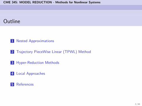
Outline
1 Nested Approximations
2 Trajectory PieceWise Linear (TPWL) Method
3 Hyper-Reduction Methods
4 Local Approaches
5 References
2 / 65
CME 345: MODEL REDUCTION - Methods for Nonlinear Systems
Nested Approximations
Nonlinear HDM
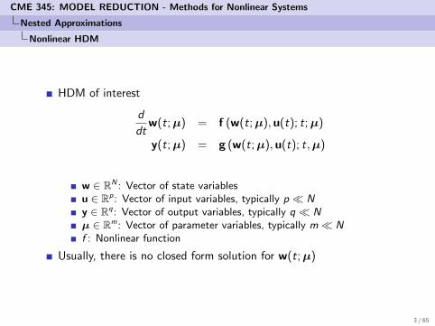
HDM of interest
d
dtw(t;µ) = f (w(t;µ),u(t); t;µ)
y(t;µ) = g (w(t;µ),u(t); t,µ)
w ∈ RN : Vector of state variablesu ∈ Rp: Vector of input variables, typically p � Ny ∈ Rq: Vector of output variables, typically q � Nµ ∈ Rm: Vector of parameter variables, typically m� Nf : Nonlinear function
Usually, there is no closed form solution for w(t;µ)
3 / 65
CME 345: MODEL REDUCTION - Methods for Nonlinear Systems
Nested Approximations
Model Order Reduction by Petrov-Galerkin Projection
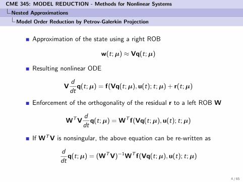
Approximation of the state using a right ROB
w(t;µ) ≈ Vq(t;µ)
Resulting nonlinear ODE
Vd
dtq(t;µ) = f(Vq(t;µ),u(t); t;µ) + r(t;µ)
Enforcement of the orthogonality of the residual r to a left ROB W
WTVd
dtq(t;µ) = WT f(Vq(t;µ),u(t); t;µ)
If WTV is nonsingular, the above equation can be re-written as
d
dtq(t;µ) = (WTV)−1WT f(Vq(t;µ),u(t); t;µ)
4 / 65
CME 345: MODEL REDUCTION - Methods for Nonlinear Systems
Nested Approximations
An Issue with the Reduction of Nonlinear Models
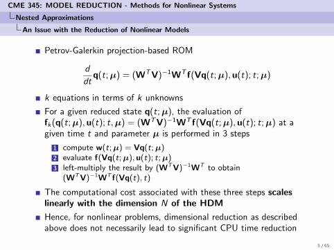
Petrov-Galerkin projection-based ROM
d
dtq(t;µ) = (WTV)−1WT f(Vq(t;µ),u(t); t;µ)
k equations in terms of k unknowns
For a given reduced state q(t;µ), the evaluation offk(q(t;µ),u(t); t,µ) = (WTV)−1WT f(Vq(t;µ),u(t); t;µ) at agiven time t and parameter µ is performed in 3 steps
1 compute w(t;µ) = Vq(t;µ)2 evaluate f(Vq(t;µ), u(t); t;µ)3 left-multiply the result by (WTV)−1WT to obtain
(WTV)−1WT f(Vq(t), t)
The computational cost associated with these three steps scaleslinearly with the dimension N of the HDM
Hence, for nonlinear problems, dimensional reduction as describedabove does not necessarily lead to significant CPU time reduction
5 / 65
CME 345: MODEL REDUCTION - Methods for Nonlinear Systems
Nested Approximations
Nested Approximations
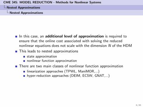
In this case, an additional level of approximation is required toensure that the online cost associated with solving the reducednonlinear equations does not scale with the dimension N of the HDM
This leads to nested approximations
state approximationnonlinear function approximation
There are two main classes of nonlinear function approximation
linearization approaches (TPWL, ManiMOR,...)hyper-reduction approaches (DEIM, ECSW, GNAT,...)
6 / 65
CME 345: MODEL REDUCTION - Methods for Nonlinear Systems
Trajectory PieceWise Linear (TPWL) Method
Linear Approximation of the Nonlinear Function
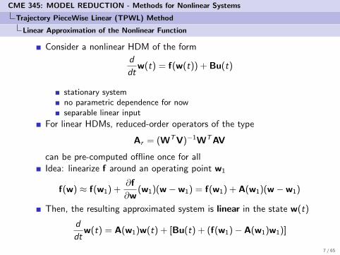
Consider a nonlinear HDM of the form
d
dtw(t) = f(w(t)) + Bu(t)
stationary systemno parametric dependence for nowseparable linear input
For linear HDMs, reduced-order operators of the type
Ar = (WTV)−1WTAV
can be pre-computed offline once for allIdea: linearize f around an operating point w1
f(w) ≈ f(w1) +∂f
∂w(w1)(w −w1) = f(w1) + A(w1)(w −w1)
Then, the resulting approximated system is linear in the state w(t)
d
dtw(t) = A(w1)w(t) + [Bu(t) + (f(w1)− A(w1)w1)]
7 / 65
CME 345: MODEL REDUCTION - Methods for Nonlinear Systems
Trajectory PieceWise Linear (TPWL) Method
Model Order Reduction
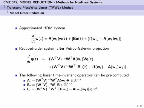
Approximated HDM system
d
dtw(t) = A(w1)w(t) + [Bu(t) + (f(w1)− A(w1)w1)]
Reduced-order system after Petrov-Galerkin projection
d
dtq(t) = (WTV)−1WTA(w1)Vq(t)
+(WTV)−1WT [Bu(t) + (f(w1)− A(w1)w1)]
The following linear time-invariant operators can be pre-computed
Ar = (WTV)−1WTA(w1)V ∈ Rk×k
Br = (WTV)−1WTB ∈ Rk×p
Fr = (WTV)−1WT [(f(w1)− A(w1)w1)] ∈ Rk
8 / 65
CME 345: MODEL REDUCTION - Methods for Nonlinear Systems
Trajectory PieceWise Linear (TPWL) Method
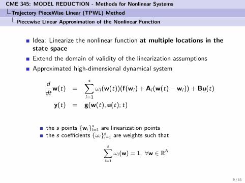
Piecewise Linear Approximation of the Nonlinear Function
Idea: Linearize the nonlinear function at multiple locations in thestate space
Extend the domain of validity of the linearization assumptions
Approximated high-dimensional dynamical system
d
dtw(t) =
s∑i=1
ωi (w(t))(f(wi ) + Ai (w(t)−wi )) + Bu(t)
y(t) = g(w(t),u(t); t)
the s points {wi}si=1 are linearization pointsthe s coefficients {ωi}si=1 are weights such that
s∑i=1
ωi (w) = 1, ∀w ∈ RN
9 / 65
CME 345: MODEL REDUCTION - Methods for Nonlinear Systems
Trajectory PieceWise Linear (TPWL) Method
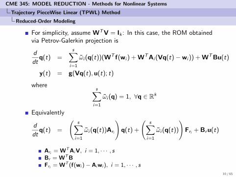
Reduced-Order Modeling
For simplicity, assume WTV = Ik : In this case, the ROM obtainedvia Petrov-Galerkin projection is
d
dtq(t) =
s∑i=1
ωi (q(t))(WT f(wi ) + WTAi (Vq(t)−wi )) + WTBu(t)
y(t) = g(Vq(t),u(t); t)
wheres∑
i=1
ωi (q) = 1, ∀q ∈ Rk
Equivalently
d
dtq(t) =
(s∑
i=1
ωi (q(t))Ari
)q(t) +
(s∑
i=1
ωi (q(t))
)Fri + Bru(t)
Ari = WTAiV, i = 1, · · · , sBr = WTBFri = WT (f(wi )− Aiwi ), i = 1, · · · , s
10 / 65
CME 345: MODEL REDUCTION - Methods for Nonlinear Systems
Trajectory PieceWise Linear (TPWL) Method
Reduced-Order Modeling
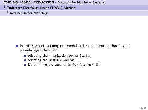
In this context, a complete model order reduction method shouldprovide algorithms for
selecting the linearization points {wi}si=1
selecting the ROBs V and WDetermining the weights {ωi (q)}si=1, ∀q ∈ Rk
11 / 65
CME 345: MODEL REDUCTION - Methods for Nonlinear Systems
Trajectory PieceWise Linear (TPWL) Method
Selection of the Linearization Points
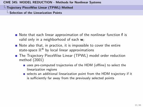
Note that each linear approximation of the nonlinear function f isvalid only in a neighborhood of each wi
Note also that, in practice, it is impossible to cover the entirestate-space RN by local linear approximations
The Trajectory PieceWise Linear (TPWL) model order reductionmethod (2001)
uses pre-computed trajectories of the HDM (offline) to select thelinearization regionsselects an additional linearization point from the HDM trajectory if itis sufficiently far away from the previously selected points
12 / 65
CME 345: MODEL REDUCTION - Methods for Nonlinear Systems
Trajectory PieceWise Linear (TPWL) Method
Selection of the ROBs
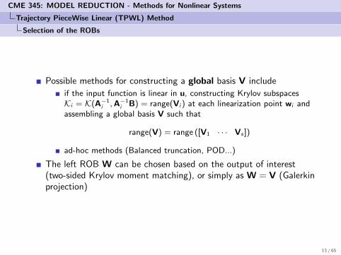
Possible methods for constructing a global basis V include
if the input function is linear in u, constructing Krylov subspacesKi = K(A−1
i ,A−1i B) = range(Vi ) at each linearization point wi and
assembling a global basis V such that
range(V) = range ([V1 · · · Vs ])
ad-hoc methods (Balanced truncation, POD...)
The left ROB W can be chosen based on the output of interest(two-sided Krylov moment matching), or simply as W = V (Galerkinprojection)
13 / 65
CME 345: MODEL REDUCTION - Methods for Nonlinear Systems
Trajectory PieceWise Linear (TPWL) Method
Determination of the Weights {ωi}
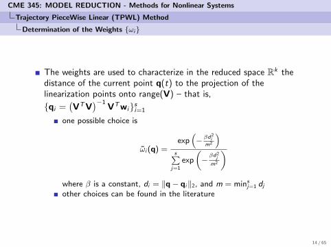
The weights are used to characterize in the reduced space Rk thedistance of the current point q(t) to the projection of thelinearization points onto range(V) – that is,
{qi =(VTV
)−1VTwi}si=1
one possible choice is
ωi (q) =exp
(−βd
2i
m2
)s∑
j=1
exp
(−βd2jm2
)where β is a constant, di = ‖q− qi‖2, and m = mins
j=1 djother choices can be found in the literature
14 / 65
CME 345: MODEL REDUCTION - Methods for Nonlinear Systems
Trajectory PieceWise Linear (TPWL) Method
Further Developments
A posteriori error estimators are available when f is negativemonotone
Stability guarantee is possible under some assumptions on f andspecific choices for V and the weights {ωi (q)}si=1
Passivity preservation (i.e. no energy creation in a passive system) ispossible under similar assumptions
TPWL using local ROBs (ManiMOR)
15 / 65
CME 345: MODEL REDUCTION - Methods for Nonlinear Systems
Trajectory PieceWise Linear (TPWL) Method
Analysis of the TPWL Method
Strengths
The cost of the online phasedoes not scale with the sizeN of the HDM
The online phase is notsoftware-intrusive
Weaknesses
It is essential to choose goodlinearization points offline
Requires the extraction ofJacobians from the HDMsoftware
Many parameters to adjust(number of linearizationpoints, weights, ...)
16 / 65
CME 345: MODEL REDUCTION - Methods for Nonlinear Systems
Hyper-Reduction Methods
The Gappy POD
First applied to face recognition (Emerson and Sirovich,“Karhunen-Loeve Procedure for Gappy Data”, 1996)
Other applications
flow sensing and estimationflow reconstructionnonlinear model order reduction
17 / 65
CME 345: MODEL REDUCTION - Methods for Nonlinear Systems
Hyper-Reduction Methods
The Gappy POD
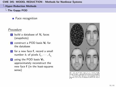
Face recognition
Procedure
1 build a database of Ns faces(snapshots)
2 construct a POD basis Vf forthe database
3 for a new face f, record a smallnumber ki of pixels fi1 , · · · , fiki
4 using the POD basis Vf ,approximately reconstruct thenew face f (in the least-squaressense)
18 / 65
CME 345: MODEL REDUCTION - Methods for Nonlinear Systems
Hyper-Reduction Methods
Nonlinear Function Approximation by Gappy POD
The gappy approach can also be used to approximate the nonlinearfunction f in the reduced equations
d
dtq(t) = WT f(Vq(t); t)
(for simplicity, the input function u(t) is not considered here)
The evaluation of all the entries of f(·; t) is computationallyexpensive (scales with N)
Gappy approach
only a small subset of these entries is evaluatedthe other entries are reconstructed either by interpolation or aleast-squares strategy using a pre-computed ROB Vf
The dimension of the solution space is still reduced using anypreferred model order reduction method (for example, POD)
19 / 65
CME 345: MODEL REDUCTION - Methods for Nonlinear Systems
Hyper-Reduction Methods
Nonlinear Function Approximation by Gappy POD
A complete model order reduction method based on the Gappyapproach should then provide algorithms for
selecting the evaluation entries I = {i1, · · · , iki }selecting a reduced-order basis Vf for the nonlinear function freconstructing the complete approximated nonlinear function f(·; t)
20 / 65
CME 345: MODEL REDUCTION - Methods for Nonlinear Systems
Hyper-Reduction Methods
Construction of a POD Basis for f
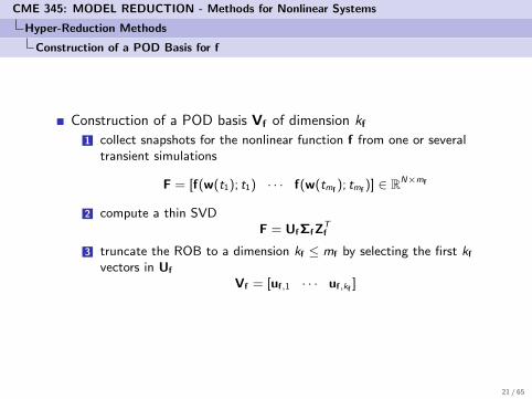
Construction of a POD basis Vf of dimension kf
1 collect snapshots for the nonlinear function f from one or severaltransient simulations
F = [f(w(t1); t1) · · · f(w(tmf ); tmf )] ∈ RN×mf
2 compute a thin SVDF = Uf Σf Z
Tf
3 truncate the ROB to a dimension kf ≤ mf by selecting the first kf
vectors in Uf
Vf = [uf,1 · · · uf,kf ]
21 / 65
CME 345: MODEL REDUCTION - Methods for Nonlinear Systems
Hyper-Reduction Methods
Reconstruction of an Approximated Nonlinear Function
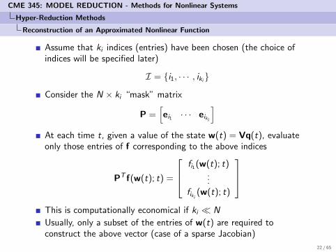
Assume that ki indices (entries) have been chosen (the choice ofindices will be specified later)
I = {i1, · · · , iki}
Consider the N × ki “mask” matrix
P =[ei1 · · · eiki
]At each time t, given a value of the state w(t) = Vq(t), evaluateonly those entries of f corresponding to the above indices
PT f(w(t); t) =
fi1(w(t); t)...
fiki (w(t); t)
This is computationally economical if ki � N
Usually, only a subset of the entries of w(t) are required toconstruct the above vector (case of a sparse Jacobian)
22 / 65
CME 345: MODEL REDUCTION - Methods for Nonlinear Systems
Hyper-Reduction Methods
Discrete Empirical Interpolation Method (DEIM)
Case where ki = kf ⇒ interpolationidea: fij (w; t) = fij (w; t), ∀w ∈ RN , ∀j = 1, · · · , kithis means that
PT f(w(t); t) = PT f(w(t); t)
recalling that f(·; t) belongs to the range of Vf – that is,
f(Vq(t); t) = Vf fr (q(t); t), where fr (q(t); t) ∈ Rkf
thenPTVf fr (q(t); t) = PT f(Vq(t); t)
assuming that PTVf is nonsingular
fr (q(t); t) = (PTVf )−1PT f(Vq(t); t)
interpolating the high-dimensional nonlinear function f(·; t) as follows
f(·; t) = Vf (PTVf )−1PT f(·; t) = ΠVf ,Pf(·; t)
the Discrete Empirical Interpolation Method (DEIM) results in anoblique projection of the high-dimensional nonlinear vector
23 / 65
CME 345: MODEL REDUCTION - Methods for Nonlinear Systems
Hyper-Reduction Methods
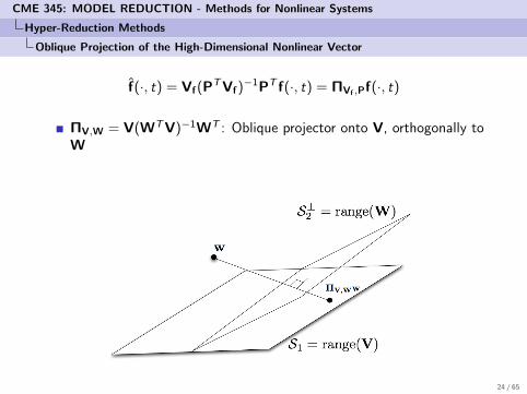
Oblique Projection of the High-Dimensional Nonlinear Vector
f(·, t) = Vf(PTVf)−1PT f(·, t) = ΠVf ,Pf(·, t)
ΠV,W = V(WTV)−1WT : Oblique projector onto V, orthogonally toW
24 / 65
CME 345: MODEL REDUCTION - Methods for Nonlinear Systems
Hyper-Reduction Methods
Least-Squares Reconstruction
Case where ki > kf ⇒ least-squares reconstructionidea: fij (w; t) ≈ fij (w; t), ∀w ∈ RN , ∀j = 1, · · · ,N, in theleast-squares sensethis leads to the minimization problem
fr (q(t); t) = argminyr∈Rkf
‖PTVfyr − PT f(Vq(t); t)‖2
note that M = PTVf ∈ Rki×kf is a skinny matrixits singular value decomposition can be written as
M = UΣZT
then, the left inverse of M can be defined as
M† = ZΣ†UT
where Σ† = diag( 1σ1, · · · , 1
σr, 0, · · · , 0) if
Σ = diag(σ1, · · · , σr , 0, · · · , 0), where σ1 ≥ · · ·σr > 0and therefore
f(q(t); t) = Vf
(ZӆUT
)PT f(Vq(t); t)
= Vf
(PTVf
)†PT f(Vq(t); t)
25 / 65
CME 345: MODEL REDUCTION - Methods for Nonlinear Systems
Hyper-Reduction Methods
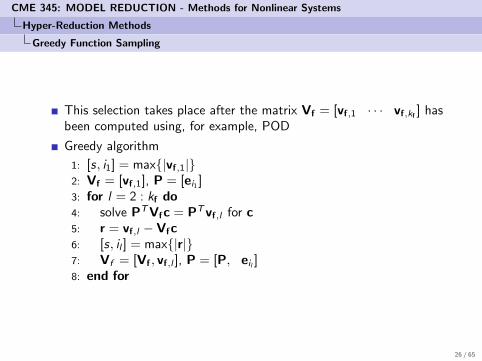
Greedy Function Sampling
This selection takes place after the matrix Vf = [vf,1 · · · vf,kf ] hasbeen computed using, for example, POD
Greedy algorithm
1: [s, i1] = max{|vf,1|}2: Vf = [vf,1], P = [ei1 ]3: for l = 2 : kf do4: solve PTVfc = PTvf,l for c5: r = vf,l − Vfc6: [s, il ] = max{|r|}7: Vf = [Vf , vf,l ], P = [P, eil ]8: end for
26 / 65
CME 345: MODEL REDUCTION - Methods for Nonlinear Systems
Hyper-Reduction Methods
Analysis of Hyper-Reduction Methods
Strengths
The cost of the online phasedoes not scale with the sizeN of the HDM
The hyper-reduced functionis usually robust with respectto deviations from theoriginal training trajectory
Weaknesses
The online phase issoftware-intrusive
Many parameters to adjust(ROB sizes, mask size, ...)
27 / 65
CME 345: MODEL REDUCTION - Methods for Nonlinear Systems
Hyper-Reduction Methods
Application to the Reduction of the Burgers Equation
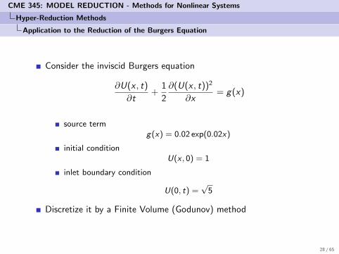
Consider the inviscid Burgers equation
∂U(x , t)
∂t+
1
2
∂(U(x , t))2
∂x= g(x)
source termg(x) = 0.02 exp(0.02x)
initial conditionU(x , 0) = 1
inlet boundary condition
U(0, t) =√
5
Discretize it by a Finite Volume (Godunov) method
28 / 65
CME 345: MODEL REDUCTION - Methods for Nonlinear Systems
Hyper-Reduction Methods
Application to the Reduction of the Burgers Equation
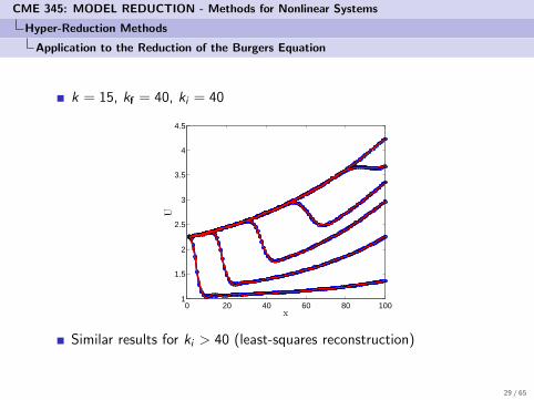
k = 15, kf = 40, ki = 40
0 20 40 60 80 1001
1.5
2
2.5
3
3.5
4
4.5
x
U
Similar results for ki > 40 (least-squares reconstruction)
29 / 65

CME 345: MODEL REDUCTION - Methods for Nonlinear Systems
Hyper-Reduction Methods
Application to the Reduction of the Burgers Equation
Results of the greedy algorithm
0 20 40 60 80 100 120−1
−0.8
−0.6
−0.4
−0.2
0
0.2
0.4
0.6
0.8
1Index Greedy Selection
1 23 4 56 78910 111213 1415 161718 192021 22 23 242526 27 2829 30
30 / 65
CME 345: MODEL REDUCTION - Methods for Nonlinear Systems
Hyper-Reduction Methods
Application to the Reduction of the Burgers Equation
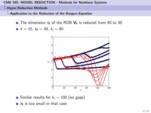
The dimension kf of the ROB Vf is reduced from 40 to 30
k = 15, kf = 30, ki = 80
0 20 40 60 80 100−1
0
1
2
3
4
5
x
U
Similar results for ki = 100 (no gaps)
kf is too small in that case
31 / 65
CME 345: MODEL REDUCTION - Methods for Nonlinear Systems
Hyper-Reduction Methods
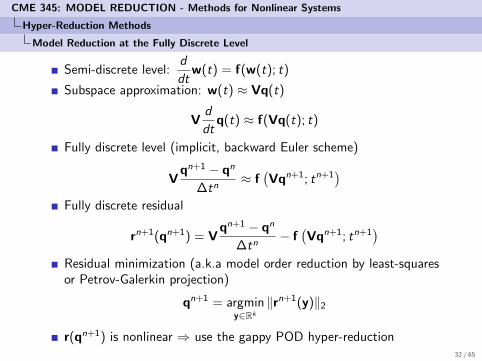
Model Reduction at the Fully Discrete Level
Semi-discrete level:d
dtw(t) = f(w(t); t)
Subspace approximation: w(t) ≈ Vq(t)
Vd
dtq(t) ≈ f(Vq(t); t)
Fully discrete level (implicit, backward Euler scheme)
Vqn+1 − qn
∆tn≈ f
(Vqn+1; tn+1
)Fully discrete residual
rn+1(qn+1) = Vqn+1 − qn
∆tn− f(Vqn+1; tn+1
)Residual minimization (a.k.a model order reduction by least-squaresor Petrov-Galerkin projection)
qn+1 = argminy∈Rk
‖rn+1(y)‖2
r(qn+1) is nonlinear ⇒ use the gappy POD hyper-reduction32 / 65
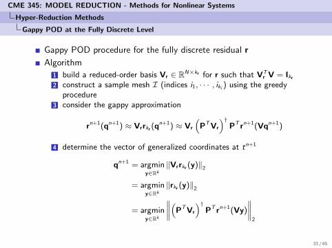
CME 345: MODEL REDUCTION - Methods for Nonlinear Systems
Hyper-Reduction Methods
Gappy POD at the Fully Discrete Level
Gappy POD procedure for the fully discrete residual r
Algorithm
1 build a reduced-order basis Vr ∈ RN×kr for r such that VTr V = Ikr
2 construct a sample mesh I (indices i1, · · · , iki ) using the greedyprocedure
3 consider the gappy approximation
rn+1(qn+1) ≈ Vrrkr (qn+1) ≈ Vr
(PTVr
)†PT rn+1(Vqn+1)
4 determine the vector of generalized coordinates at tn+1
qn+1 = argminy∈Rk
‖Vrrkr (y)‖2
= argminy∈Rk
‖rkr (y)‖2
= argminy∈Rk
∥∥∥∥(PTVr
)†PT rn+1(Vy)
∥∥∥∥2
33 / 65
CME 345: MODEL REDUCTION - Methods for Nonlinear Systems
Hyper-Reduction Methods
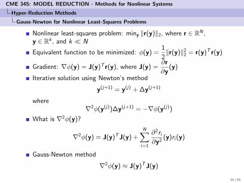
Gauss-Newton for Nonlinear Least-Squares Problems
Nonlinear least-squares problem: miny ‖r(y)‖2, where r ∈ RN ,y ∈ Rk , and k � N
Equivalent function to be minimized: φ(y) =1
2‖r(y)‖22 = r(y)T r(y)
Gradient: ∇φ(y) = J(y)T r(y), where J(y) =∂r
∂y(y)
Iterative solution using Newton’s method
y(j+1) = y(j) + ∆y(j+1)
where∇2φ(y(j))∆y(j+1) = −∇φ(y(j))
What is ∇2φ(y)?
∇2φ(y) = J(y)TJ(y) +N∑i=1
∂2ri∂y2
(y)ri (y)
Gauss-Newton method
∇2φ(y) ≈ J(y)TJ(y)
34 / 65
CME 345: MODEL REDUCTION - Methods for Nonlinear Systems
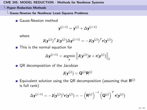
Hyper-Reduction Methods
Gauss-Newton for Nonlinear Least-Squares Problems
Gauss-Newton method
y(j+1) = y(j) + ∆y(j+1)
whereJ(y(j))TJ(y(j))∆y(j+1) = −J(y(j))T r(y(j))
This is the normal equation for
∆y(j+1) = argminz
∥∥∥J(y(j))z + r(y(j))∥∥∥2
QR decomposition of the Jacobian
J(y(j)) = Q(j)R(j)
Equivalent solution using the QR decomposition (assuming that R(j)
is full rank)
∆y(j+1) = −J(y(j))†r(y(j)) = −(
R(j))−1 (
Q(j))T
r(y(j))
35 / 65
CME 345: MODEL REDUCTION - Methods for Nonlinear Systems
Hyper-Reduction Methods
Gauss-Newton with Approximated Tensors
GNAT (Gauss-Newton with Approximated Tensors) =Gauss-Newton + gappy PODMinimization problem
miny∈Rk
∥∥∥(PTVr
)†PT rn+1(Vy)
∥∥∥2
Jacobian: J(y) =(PTVr
)†PTJn+1(Vy)
Define a small dimensional operator (and construct it offline)
A =(PTVr
)†Least-squares problem at Gauss-Newton iteration j of tn+1
∆y(j) = argminz∈Rk
∥∥∥APTJn+1(Vy(j))Vz + APT rn+1(Vy(j))∥∥∥2
GNAT solution using QR
APTJn+1(Vy(j))V = Q(j)R(j)
∆y(j) = −(
R(j))−1 (
Q(j))T
APT rn+1(Vy(j))
36 / 65
CME 345: MODEL REDUCTION - Methods for Nonlinear Systems
Hyper-Reduction Methods
Gauss-Newton with Approximated Tensors
Further developments
concept of a reduced meshconcept of an output mesherror boundsGNAT using local reduced-order bases
37 / 65
CME 345: MODEL REDUCTION - Methods for Nonlinear Systems
Hyper-Reduction Methods
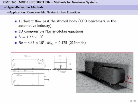
Application: Compressible Navier-Stokes Equations
Turbulent flow past the Ahmed body (CFD benchmark in theautomotive industry)
3D compressible Navier-Stokes equations
N = 1.73× 10⁷
Re = 4.48× 10⁶, M∞ = 0.175 (216km/h)
38 / 65
CME 345: MODEL REDUCTION - Methods for Nonlinear Systems
Hyper-Reduction Methods
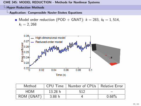
Application: Compressible Navier-Stokes Equations
Model order reduction (POD + GNAT): k = 283, kf = 1, 514,ki = 2, 268
Method CPU Time Number of CPUs Relative Error
HDM 13.28 h 512 –ROM (GNAT) 3.88 h 4 0.68%
39 / 65
CME 345: MODEL REDUCTION - Methods for Nonlinear Systems
Hyper-Reduction Methods
Application: Compressible Navier-Stokes Equations
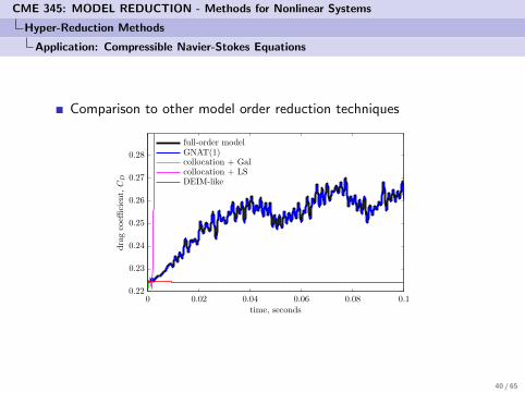
Comparison to other model order reduction techniques
DEIM-likecollocation + LScollocation + GalGNAT(1)full-order model
dragcoeffi
cient,
CD
time, seconds0 0.02 0.04 0.06 0.08 0.1
0.22
0.23
0.24
0.25
0.26
0.27
0.28
40 / 65
CME 345: MODEL REDUCTION - Methods for Nonlinear Systems
Hyper-Reduction Methods
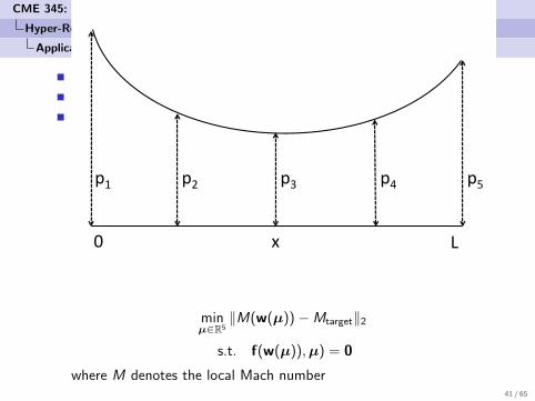
Application: Design Optimization of a Nozzle
HDM: N = 2, 048, m = 5 shape parameters
Model order reduction (POD + DEIM): k = 8, kf = 20, ki = 20
Steady, parameterized problem
p3
x 0 L
p1 p2 p4 p5
minµ∈R5
‖M(w(µ))−Mtarget‖2
s.t. f(w(µ)),µ) = 0
where M denotes the local Mach number41 / 65
CME 345: MODEL REDUCTION - Methods for Nonlinear Systems
Hyper-Reduction Methods
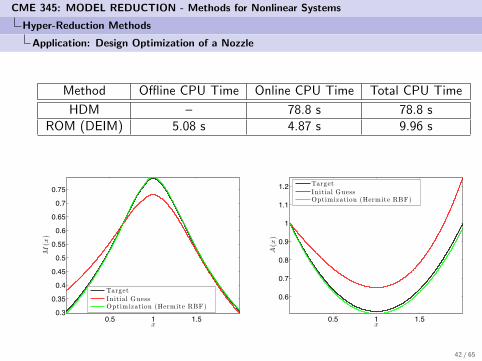
Application: Design Optimization of a Nozzle
Method Offline CPU Time Online CPU Time Total CPU Time
HDM – 78.8 s 78.8 sROM (DEIM) 5.08 s 4.87 s 9.96 s
0.5 1 1.50.3
0.35
0.4
0.45
0.5
0.55
0.6
0.65
0.7
0.75
x
M(x
)
TargetInitial GuessOptimization (Hermite RBF)
0.5 1 1.5
0.6
0.7
0.8
0.9
1
1.1
1.2
x
A(x
)
TargetInitial GuessOptimization (Hermite RBF)
42 / 65
CME 345: MODEL REDUCTION - Methods for Nonlinear Systems
Local Approaches
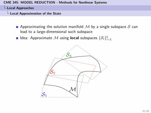
Local Approximation of the State
Approximating the solution manifold M by a single subspace S canlead to a large-dimensional such subspace
Idea: Approximate M using local subspaces {Sl}Li=1
MS1
S2
S3
43 / 65

CME 345: MODEL REDUCTION - Methods for Nonlinear Systems
Local Approaches
Local Approximation of the State
In practice, the local approximation of the state takes place at thefully discrete level
Each local subspace Sl is associated with a local ROB Vl
At each time-step n, the state wn is computed as
wn = wn−1 + ∆wn
The increment ∆wn is then approximated in a subspaceSl,n = range(Vl,n) as
∆wn ≈ Vl,nqn
The choice of the reduced-order basis Vl,n is specified later
By induction, the state wn is computed as
wn = w0 +n∑
i=1
Vl,i qn
44 / 65
CME 345: MODEL REDUCTION - Methods for Nonlinear Systems
Local Approaches
Local Approximation of the State
The state wn is computed as
wn = w0 +n∑
i=1
Vl,i qn
In practice, the ROBs {Vl,i}ni=1 are chosen among a finite set oflocal ROBs {Vl}Ll=1
Hence
wn = w0 +L∑
l=1
Vlqnl
This shows that
wn ∈ w0 + range([V1 · · · VV ])
Note that each local ROB can be of a different dimension
Vl ∈ RN×kl
45 / 65
CME 345: MODEL REDUCTION - Methods for Nonlinear Systems
Local Approaches
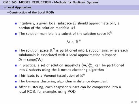
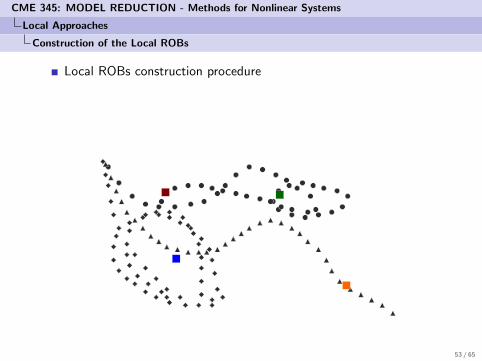
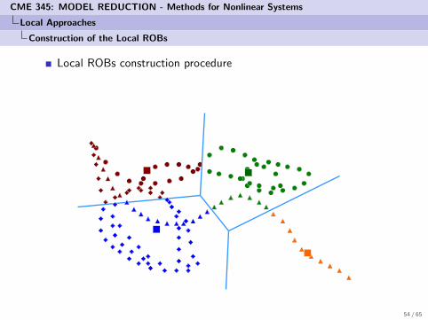
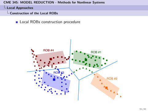
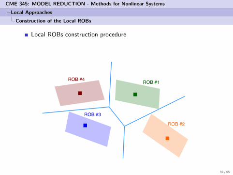
Construction of the Local ROBs
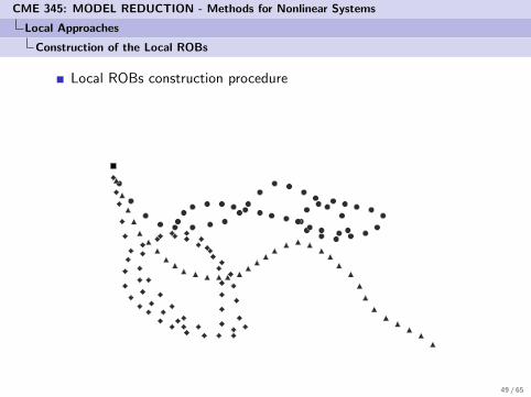
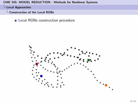
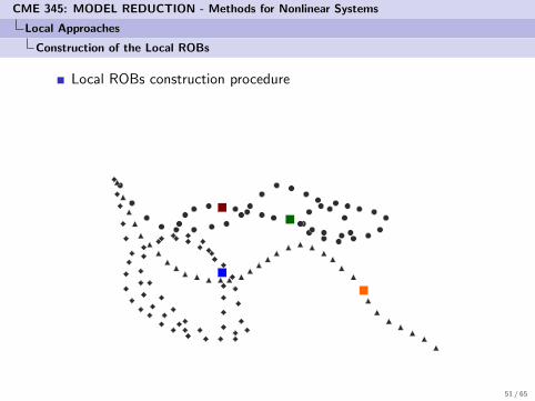
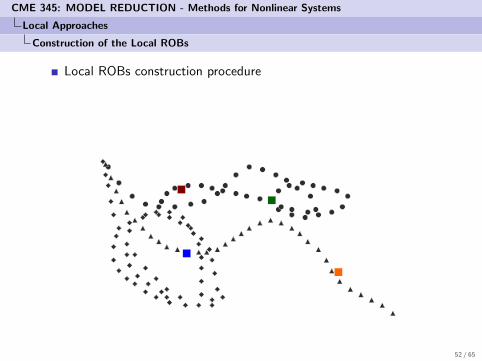
Intuitively, a given local subspace Sl should approximate only aportion of the solution manifold MThe solution manifold is a subset of the solution space RN
M⊂ RN
The solution space RN is partitioned into L subdomains, where eachsubdomain is associated with a local approximation subspaceSl = range(Vl)
In practice, a set of solution snapshots {wi}Ns
i=1 can be partitionedinto L subsets using the k-means clustering algorithm
This leads to a Voronoi tessellation of RN
The k-means clustering algorithm is distance dependent
After clustering, each snapshot subset can be compressed into alocal ROB, for example, using POD
46 / 65
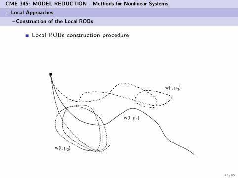
CME 345: MODEL REDUCTION - Methods for Nonlinear Systems
Local Approaches
Construction of the Local ROBs
Local ROBs construction procedure
w(t, µ1)!
w(t, µ2)!
w(t, µ3)!
47 / 65
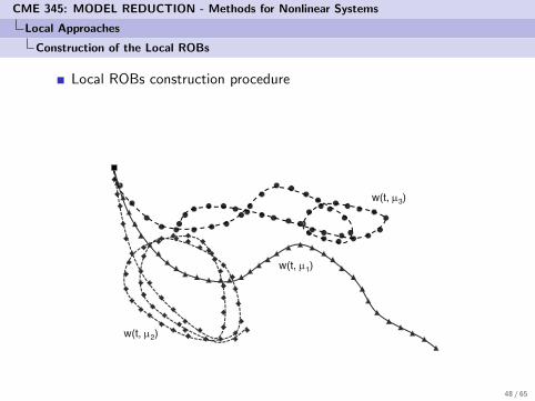
CME 345: MODEL REDUCTION - Methods for Nonlinear Systems
Local Approaches
Construction of the Local ROBs
Local ROBs construction procedure
w(t, µ1)!
w(t, µ2)!
w(t, µ3)!
48 / 65
CME 345: MODEL REDUCTION - Methods for Nonlinear Systems
Local Approaches
Construction of the Local ROBs
Local ROBs construction procedure
49 / 65
CME 345: MODEL REDUCTION - Methods for Nonlinear Systems
Local Approaches
Construction of the Local ROBs
Local ROBs construction procedure
50 / 65
CME 345: MODEL REDUCTION - Methods for Nonlinear Systems
Local Approaches
Construction of the Local ROBs
Local ROBs construction procedure
51 / 65
CME 345: MODEL REDUCTION - Methods for Nonlinear Systems
Local Approaches
Construction of the Local ROBs
Local ROBs construction procedure
52 / 65
CME 345: MODEL REDUCTION - Methods for Nonlinear Systems
Local Approaches
Construction of the Local ROBs
Local ROBs construction procedure
53 / 65
CME 345: MODEL REDUCTION - Methods for Nonlinear Systems
Local Approaches
Construction of the Local ROBs
Local ROBs construction procedure
54 / 65
CME 345: MODEL REDUCTION - Methods for Nonlinear Systems
Local Approaches
Construction of the Local ROBs
Local ROBs construction procedure
ROB #1!
ROB #2!
ROB #3!
ROB #4!
55 / 65
CME 345: MODEL REDUCTION - Methods for Nonlinear Systems
Local Approaches
Construction of the Local ROBs
Local ROBs construction procedure
ROB #1!
ROB #2!
ROB #3!
ROB #4!
56 / 65
CME 345: MODEL REDUCTION - Methods for Nonlinear Systems
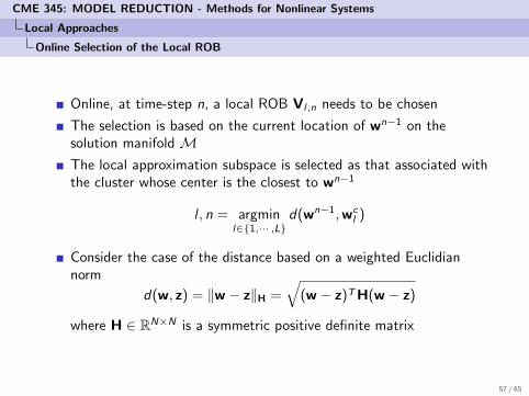
Local Approaches
Online Selection of the Local ROB
Online, at time-step n, a local ROB Vl,n needs to be chosen
The selection is based on the current location of wn−1 on thesolution manifold MThe local approximation subspace is selected as that associated withthe cluster whose center is the closest to wn−1
l , n = argminl∈{1,··· ,L}
d(wn−1,wcl )
Consider the case of the distance based on a weighted Euclidiannorm
d(w, z) = ‖w − z‖H =√
(w − z)TH(w − z)
where H ∈ RN×N is a symmetric positive definite matrix
57 / 65
CME 345: MODEL REDUCTION - Methods for Nonlinear Systems
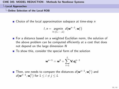
Local Approaches
Online Selection of the Local ROB
Choice of the local approximation subspace at time-step n
l , n = argminl∈{1,··· ,L}
d(wn−1,wcl )
For a distance based on a weighted Euclidian norm, the solution ofthe above problem can be computed efficiently at a cost that doesnot depend on the large dimension N
To show this, consider the special form of the solution
wn−1 = w0 +L∑
l=1
Vlqn−1l
Then, one needs to compare the distances d(wn−1,wcil ) and
d(wn−1,wcjl ) for 1 ≤ i 6= j ≤ L
58 / 65
CME 345: MODEL REDUCTION - Methods for Nonlinear Systems
Local Approaches
Online Selection of the Local ROB
The two distances d(wn−1,wcil ) and d(wn−1,w
cjl ) can be compared
as follows
∆i,j = d(wn−1,wcil )2 − d(wn−1,w
cjl )2
= ‖wn−1 −wcil ‖2H − ‖wn−1 −w
cjl ‖2H
= ‖L∑
l=1
Vlqn−1l ‖2H + ‖wci
l −w0‖2H − 2L∑
l=1
[wci ]TVlqn−1l
−‖L∑
l=1
Vlqn−1l ‖2H − ‖w
cjl −w0‖2H + 2
L∑l=1
[wcj ]TVlqn−1l
= ‖wcil −w0‖2H − ‖w
cjl −w0‖2H + 2
L∑l=1
[wci −wcj ]TVlqn−1l
The following small quantities can be pre-computed offline and usedonline to compute economically ∆i,j , 1 ≤ i 6= j ≤ L
ai,j = ‖wcil −w0‖2H − ‖w
cjl −w0‖2H ∈ R, gi,j = [wci −wcj ]TVl ∈ Rkl
59 / 65
CME 345: MODEL REDUCTION - Methods for Nonlinear Systems
Local Approaches
Extension to Hyper-Reduction
The local approach to nonlinear model reduction can be easilyextended to hyper-reduction as follows
The hyper-reduction approach is applied independently to eachsubset of snapshots
It leads to the definition of
the local ROBs for the state: Vl , l = 1, · · · , Lthe local ROBs for the residual: Vr,l , l = 1, · · · , Lthe local masks: Il , l = 1, · · · , L
The choice of the local ROBs and masks is still dictated by thelocation of the current time-iterate in the state space
60 / 65
CME 345: MODEL REDUCTION - Methods for Nonlinear Systems
Local Approaches
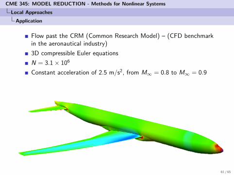
Application
Flow past the CRM (Common Research Model) – (CFD benchmarkin the aeronautical industry)
3D compressible Euler equations
N = 3.1× 10⁶
Constant acceleration of 2.5 m/s2, from M∞ = 0.8 to M∞ = 0.9
61 / 65
CME 345: MODEL REDUCTION - Methods for Nonlinear Systems
Local Approaches
Application
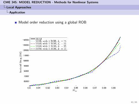
Model order reduction using a global ROB
62 / 65
CME 345: MODEL REDUCTION - Methods for Nonlinear Systems
Local Approaches
Application
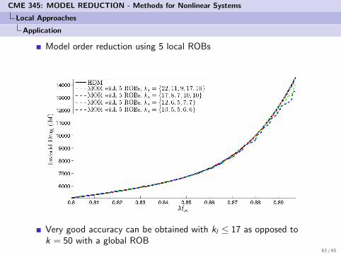
Model order reduction using 5 local ROBs
Very good accuracy can be obtained with kl ≤ 17 as opposed tok = 50 with a global ROB
63 / 65
CME 345: MODEL REDUCTION - Methods for Nonlinear Systems
References
M. Rewienski, J. White. Model order reduction for nonlineardynamical systems based on trajectory piecewise-linearapproximations. Linear Algebra and its Applications 2006;415(2-3):426-454.
R. Everson, L. Sirovich. Karhunen–Loeve procedure for gappy data.Journal of the Optical Society of America A 1995; 12(8):1657–1664.
M. Barrault et al. An empirical interpolation method: application toefficient reduced basis discretization of partial differential equations.Comptes Rendus de lAcademie des Sciences Paris 2004;339:667–672.
K. Willcox. Unsteady flow sensing and estimation via the gappyproper orthogonal decomposition. Computers and Fluids 2006;35:208–226.
S. Chaturantabut, D.C. Sorensen. Nonlinear model reduction viaDiscrete Empirical Interpolation. SIAM Journal on ScientificComputing 2010; 32:2737–2764.
64 / 65
CME 345: MODEL REDUCTION - Methods for Nonlinear Systems
References
K. Carlberg, C. Farhat, J. Cortial, D. Amsallem. The GNAT methodfor nonlinear model reduction: effective implementation andapplication to computational fluid dynamics and turbulent flows.Journal of Computational Physics 2013; 242:623–647.K. Carlberg, C. Bou-Mosleh, C. Farhat. Efficient nonlinear modelreduction via a least-squares Petrov–Galerkin projection andcompressive tensor approximations. International Journal forNumerical Methods in Engineering 2011; 86(2):155–181.D. Amsallem, M. Zahr, Y. Choi, C. Farhat. Design optimizationusing hyper-reduced-order models. Structural and MultidisciplinaryOptimization 2015; 51:919–940.D. Amsallem, M. Zahr, C. Farhat. Nonlinear model reduction basedon local reduced order bases. International Journal for NumericalMethods in Engineering 2012; 92(12):891-916.K. Washabaugh, M. Zahr, C. Farhat, On the use of discretenonlinear reduced-order models for the prediction of steady-stateflows past parametrically deformed complex geometries.AIAA-2016-1814, AIAA SciTech 2016, San Diego, CA, January 4-8,2016. 65 / 65