Embed Size (px)
Citation preview

CMPT 431
Dr. Alexandra Fedorova
Lecture VIII: Time And Global Clocks

2CMPT 431 © A. Fedorova
A Distributed Computation With Data Dependencies
System ASystem B
System C• Ask work from System B• Compute• Send result to user
• Ask data from System C• Respond to System A
A waits for B
B waits
for C
System C became unresponsive

3CMPT 431 © A. Fedorova
Detecting and Fixing the Problem
• User gets no response from System A• How do we detect that System C is causing the problem? • Easy to detect if we get a snapshot of a global state• Constructing global state in an asynchronous distributed
system is a difficult problem

4CMPT 431 © A. Fedorova
A Naïve Approach
• Each system records each event it performed and its timestamp
• Suppose events in the this system happened in this real order:– Time Tc0: System C sent data to System B (before C stopped
responding)– Time Ta0: System A asked for work from System B – Time Tb0: System B asked for data from System C
Tc0 Ta0 Tb0

5CMPT 431 © A. Fedorova
A Naïve Approach (cont)
• Ideally, we will construct real order of events from local timestamps and detect this dependency chain:
System A
System B
System C
System C sent data
Tc
Ta
System A asked for work Tb
System B asked for data

6CMPT 431 © A. Fedorova
A Naïve Approach (cont)
• But in reality, we do not know if Tc occurred before Ta and Tb, because in an asynchronous distributed system clocks are not synchronized!
System A
System B
System C
System C sent data
Tc
Ta
System A asked for work Tb
System B asked for data
System C sent data
Tc

7CMPT 431 © A. Fedorova
This Lecture’s Topic
• We will learn how to solve this problem in an asynchronous distributed system
• Our goal is to construct a consistent global state in presence of unsynchronized local clocks
• We will begin by creating a formal model for– Distributed computation– Event precedence in a distributed computation
• We will use event precedence model to define consistent global state
• Then we will learn to construct consistent global states

8CMPT 431 © A. Fedorova
Model of a Distributed Computation
• Collection of processes p0, …, pn
• Processes communicate by sending messages• Event send(m) enqueues message m on the sending end• Event receive(m) dequeues message m on the receiving
end• Events ei
0, ei1, … , ei
n are steps of a distributed computation at process pi
• hi = ei0, ei
1, … , ein is a local history of pi

9CMPT 431 © A. Fedorova
Events and Causal Precedence
• In an asynchronous distributed system there is no notion of global clock
• Events cannot be ordered according to some real order• We can only talk about causal event ordering, that is if
one event affects the outcome of another event• For example events send(m) and receive(m) are in causal
order, because receive(m) could not have occurred before send(m)

10CMPT 431 © A. Fedorova
Formal Rules for Ordering of Events
• If local events precede one another, then they also precede one another in the global ordering:– If ei
k ,eim Є hi and k < m, then ei
k→eim
• Sending a message always precedes receipt of that message:– If ei = send(m) and ej= receive(m), then ei→ej
• Event ordering is associative:– If e → e’ and e’ → e”, then e → e”

11CMPT 431 © A. Fedorova
Space-time Diagram of a Distributed Computation
p1e1
1 e12 e1
3 e14 e1
5 e16
p2e2
1 e22 e2
3
p3e3
1 e32 e3
3 e34 e3
5 e36
e21→e3
6 e22 || e3
6

12CMPT 431 © A. Fedorova
Cuts of a Distributed Computation
• Suppose there is an external monitor process• External monitor constructs a global state:
– Asks processes to send it local history• Global state constructed from these local histories is a
cut of a distributed computation

13CMPT 431 © A. Fedorova
Example Cuts
e11 e1
2 e13 e1
4 e15 e1
6
e21 e2
2 e23
e31 e3
2 e33 e3
4 e35 e3
6
C C’
p1
p2
p3

14CMPT 431 © A. Fedorova
Consistent vs. Inconsistent Cuts
• A cut is consistent if for any event e included in the cut, any event e’ that causally precedes e is also included in that cut
• For cut C:(e Є C) Λ (e’→ e) => e’ Є C

15CMPT 431 © A. Fedorova
Are These Cuts Consistent?
e11 e1
2 e13 e1
4 e15 e1
6
e21 e2
2 e23
e31 e3
2 e33 e3
4 e35 e3
6
C
p1
p2
p3

16CMPT 431 © A. Fedorova
Are These Cuts Consistent?
e11 e1
2 e13 e1
4 e15 e1
6
e21 e2
2 e23
e31 e3
2 e33 e3
4 e35 e3
6
C’
inconsistentincluded
in C
causally precedes e3
6
…but not included
in C

17CMPT 431 © A. Fedorova
Cuts and Global State
• Recall that our goal is to construct a consistent global state
• We’d like to get a snapshot of a distributed system as would have been observed by a perfect observer
• A consistent cut corresponds to a consistent global state• What’s next: we will learn how to construct consistent
cuts in the absence of synchronized clocks• Consistent global states can be constructed via:
– Active monitoring– Passive monitoring

18CMPT 431 © A. Fedorova
Passive vs. Active Monitoring
• Passive monitoring:– There is a process p0 external to the distributed computation
– There are processes pi (1 ≤ i ≤ n), part of the computation
– Each process pi sends to p0 a timestamp of each event it executes
• Active monitoring:– There is a process p0 external to the distributed computation
– When p0 desires to find out the state of the system it asks all processes pi to send its state

19CMPT 431 © A. Fedorova
Passive vs. Active Monitoring
• You need both passive and active monitoring• The kind of monitoring you use depends on what property of a
distributed system you are trying to detect• Passive monitoring gives you more information about the distributed
computation than active monitoring – Passive monitoring records the entire event history
• Passive monitoring uses logical clocks or vector clocks – a way to timestamp an event in the absence of global clock
• Active monitoring does not depend of special clocks, but it is also less powerful

20CMPT 431 © A. Fedorova
What Do We Need to Know to Construct a Consistent Cut?
e11 e1
2 e13 e1
4 e15 e1
6
e21 e2
2 e23
e31 e3
2 e33 e3
4 e35 e3
6
C’
inconsistentincluded
in C
causally precedes e3
6
…but not included
in CWe must know the causal ordering of events. If we
do we can detect an inconsistent cut

21CMPT 431 © A. Fedorova
Constructing a Consistent Cut Via Passive Monitoring
• We must know the causal ordering of event• If there was a global clock, we would detect this as
follows:• RC(e) – timestamp of event e given by a global clock• Clock condition:
e’→ e => RC(e) < RC(e’)• What to do if there is no global clock? • We will use logical clocks and vector clocks

22CMPT 431 © A. Fedorova
Logical Clocks
• Each process maintains a local value of a logical clock LC• Logical clock of process p counts how many events in a distributed
computation causally preceded the current event at p (including the current event).
• LC(ei) – the logical clock value at process pi at event ei
• Suppose we had a distributed system with only a single process
e11 e1
2 e13 e1
4 e15 e1
6
LC=1 LC=2 LC=3 LC=4 LC=5 LC=6

23CMPT 431 © A. Fedorova
Logical Clocks (cont.)
• In a system with more than one process logical clocks are updated as follows:
• Each message m that is sent contains a timestamp TS(m)• TS(m) is the logical clock value associated with sending
event at the sending process
e11 e1
2 e13 e1
4 e15 e1
6
LC=1 send(m)
TS(m) = 1

24CMPT 431 © A. Fedorova
Logical Clocks (cont)
• When the receiving process receives message m, it updates its logical clock to:
max{LC, TS(m)} + 1
e11 e1
2 e13 e1
4 e15 e1
6
LC=1 send(m) TS(m) = 1
e22
What is the LC value of e2
2?
LC=2
e21
LC=1

25CMPT 431 © A. Fedorova
Illustration of a Logical Clock
1 2 4 5 6 7
1 5 6
1 2 3 4 5 7
3\p1
p1
p1

26CMPT 431 © A. Fedorova
Causal Delivery with Logical Clocks
• We have a external monitor process p0
• Each process pi sends an event notification message m to p0 after each event ei
• To let p0 construct a correct causal ordering of events, we define the following delivery rule for event notification messages:
Causal delivery rule: Event notification messages are delivered to p0 in the increasing logical clock timestamp order

27CMPT 431 © A. Fedorova
Causal Delivery Rule
1 2 4 5 6 7
1 2 3 4 5 7
p1
p2
p0
m(LC=1) m(LC=2) m(LC=4)m(LC=3)
1 2 3 4

28CMPT 431 © A. Fedorova
Gap Detection Rule
1 2 4 5 6 7
1 2 3 4 5 7
p1
p2
p0
m(LC=1) m(LC=2) m(LC=4)m(LC=3)
1 2 3 4
m(LC=1)
Oops!
Must not deliver a message unless 100% sure that all messages
with smaller timestamps have been received

29CMPT 431 © A. Fedorova
Rules to Achieve Causal Delivery
• Rule #1:Do not deliver event notification message from a process pi unless all messages with smaller timestamps have been delivered (FIFO delivery)
• Rule #2:Do not deliver to p event notification message with a timestamp TS(m) unless p received messages with timestamps one smaller, equal or greater than TS(m) from all other processes
30CMPT 431 © A. Fedorova
Causal Delivery Rules
1 2 4 5 6 7
1 2 3 4 5 7
p1
p2
p0
m(LC=1) m(LC=2) m(LC=4) m(LC=3)
1
m(LC=1)
1 2

31CMPT 431 © A. Fedorova
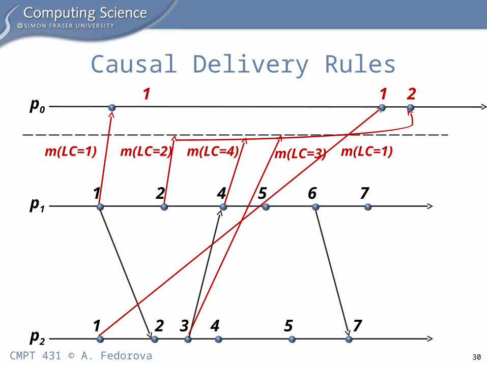
Causal Precedence Relation
• Detecting causal precedence relationship with logical clocks requires sending more than just timestamps!

32CMPT 431 © A. Fedorova
Causal Precedence or Concurrency?
1 2
1 2
p1
p2
p0
1 21 2
e11
e22
e11and e2
2are concurrent
33CMPT 431 © A. Fedorova
Causal Precedence or Concurrency?
1 2
1 2
p1
p2
p0
1 21 2
e11
e22
Now e11and e2
2are causally related
But timestamps have not changed!!!

34CMPT 431 © A. Fedorova
Causal Precedence Relation
• Using just timestamps from logical clocks does not help us detect whether two events are causally related or concurrent
• We could fix this by including a local history in the event notification message
• Not a good idea: messages will become large• A better idea: vector clocks

35CMPT 431 © A. Fedorova
Introduction to Vector Clocks
• The clock of each process is represented by a vector• The vector dimension is the number of processes in the
system• Each entry of a vector clock corresponds to a process• Suppose there are three processes: p1, p2, and p3
• Then the vector clock at each process will look like this:VC[1] – entry for process p1
VC[2] – entry for process p2
VC[3] – entry for process p3

36CMPT 431 © A. Fedorova
Using Vector Clocks
1
1 2
p1
p2
VC[1] = 0VC[2] = 0
VC[1] = 0VC[2] = 0
Initialize to 0
VC[1] = 0VC[2] = 1
VC[1] = 1VC[2] = 0
Increment local component to “1” for an internal of “send” event
VC[1] = 1VC[2] = 2
VC[1] = 1VC[2] = 0
Arrives with the message
Increment other processes’ components to be no less than at the incoming VC
Increment the local component

37CMPT 431 © A. Fedorova
The Meaning of Vector Clocks
• An entry of a vector clock for process pi is the number of events at pi
VC[1] = 3 – number of events at p1
VC[2] = 0 – number of events at p2
VC[3] = 1 – number of events at p3
• p1 knows for sure how many events it executed
• But how can it be sure about p2 and p3? It can’t!
• So p1‘s entries for p2 and p3 are...what p1 thinks about p2 and p3

38CMPT 431 © A. Fedorova
Meaning of Vector Clocks (cont)
• p1 thinks incorrectly about other processes if p1 does not communicate with other processes
• Once p1 exchanges messages with other processes, it updates its information about other processes using vector clock timestamps received from other processes

39CMPT 431 © A. Fedorova
Another Vector Clock Example
p1
p2
p3VC[1] = 0VC[2] = 0VC[3] = 1
VC[1] = 1VC[2] = 0VC[3] = 0
VC[1] = 0VC[2] = 1VC[3] = 0
VC[1] = 2VC[2] = 1VC[3] = 0
VC[1] = 1VC[2] = 0VC[3] = 2
VC[1] = 1VC[2] = 0VC[3] = 3
VC[1] = 3VC[2] = 1VC[3] = 3
VC[1] = 1VC[2] = 0VC[3] = 4
VC[1] = 1VC[2] = 2VC[3] = 4
VC[1] = 4VC[2] = 1VC[3] = 3
VC[1] = 4VC[2] = 3VC[3] = 4
VC[1] = 1VC[2] = 0VC[3] = 5
VC[1] = 5VC[2] = 1VC[3] = 3
VC[1] = 5VC[2] = 1VC[3] = 6
VC[1] = 6VC[2] = 1VC[3] = 3

40CMPT 431 © A. Fedorova
Causal Precedence or Concurrency?
1 2
1 2
p1
p2
p0
e11
e22 e1
1and e22are concurrent
VC[1] = 1VC[2] = 0
VC[1] = 0VC[2] = 1
VC[1] = 0VC[2] = 2
VC[1] = 2VC[2] = 0
VC[1] = 1VC[2] = 0
VC[1] = 0VC[2] = 1
VC[1] = 0VC[2] = 2
VC[1] = 2VC[2] = 0

41CMPT 431 © A. Fedorova
Causal Precedence or Concurrency?
1 2
1 2
p1
p2
p0
e11
e22
Now e11and
e22are causally
relatedVC[1] = 1VC[2] = 0
VC[1] = 0VC[2] = 1
VC[1] = 1VC[2] = 2
VC[1] = 2VC[2] = 0
VC[1] = 1VC[2] = 0
VC[1] = 0VC[2] = 1
VC[1] = 1VC[2] = 2
VC[1] = 2VC[2] = 0
42CMPT 431 © A. Fedorova
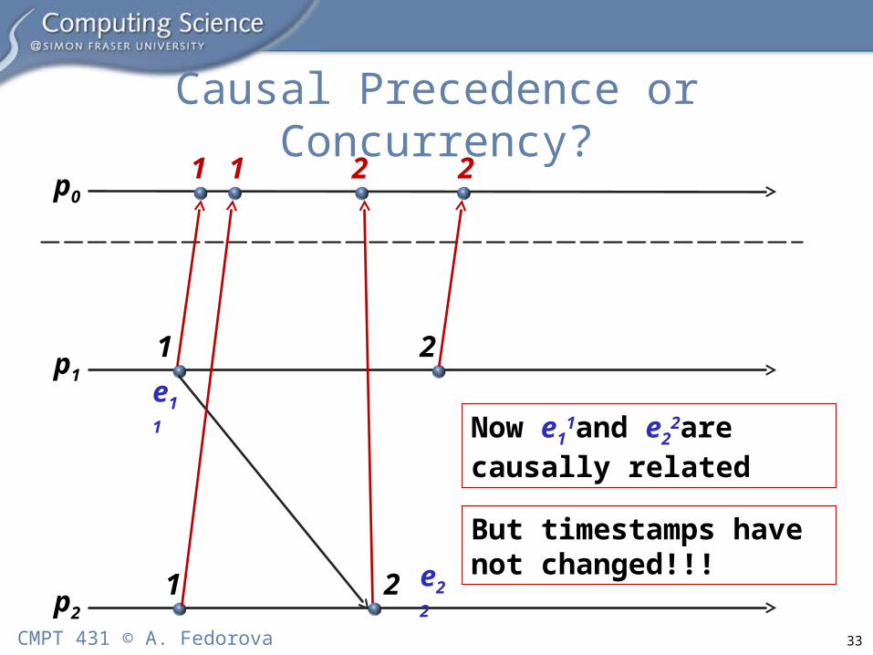
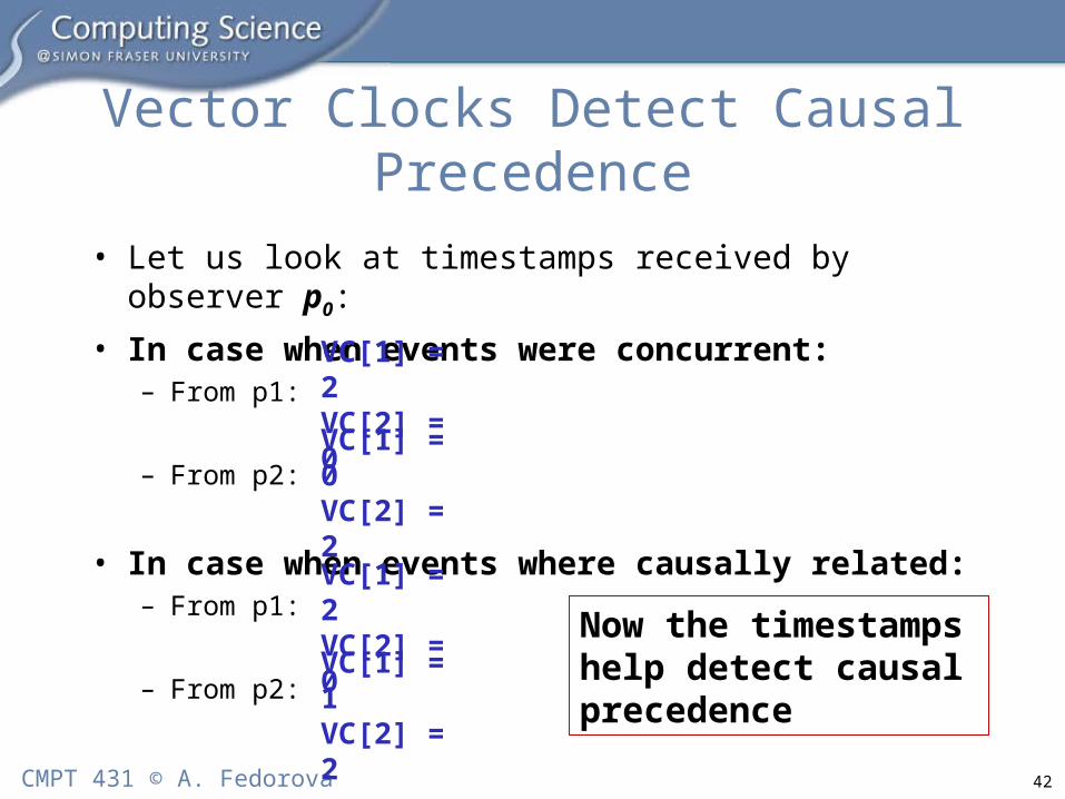
Vector Clocks Detect Causal Precedence
• Let us look at timestamps received by observer p0:• In case when events were concurrent:
– From p1:
– From p2:
• In case when events where causally related:– From p1:
– From p2:
VC[1] = 2VC[2] = 0
VC[1] = 0VC[2] = 2
VC[1] = 2VC[2] = 0
VC[1] = 1VC[2] = 2
Now the timestamps help detect causal precedence

43CMPT 431 © A. Fedorova
Use Vector Clocks to Construct Consistent Cuts
• A consistent cut is a cut that does not include pairwise inconsistent events
• So the first step is to understand pairwise inconsistency

44CMPT 431 © A. Fedorova
Informal Definition of Pairwise Inconsistency
• Look at vector timestamps of two events: ei at pi and ej at pj
• If at event ei process pi thinks that process pj executed more events than process pj thinks it has executed at event ej, the events are pairwise inconsistentExample:
timestamp at p3 timestamp at p1
– The events are pairwise inconsistent– Process p1 must know better about what it’s doing than process p3
could ever know.
VC[1] = 5VC[2] = 1VC[3] = 6
VC[1] = 4VC[2] = 1VC[3] = 3
p3 thinks that p1
has executed 5 events
p1 has
executed 4 events!
45CMPT 431 © A. Fedorova
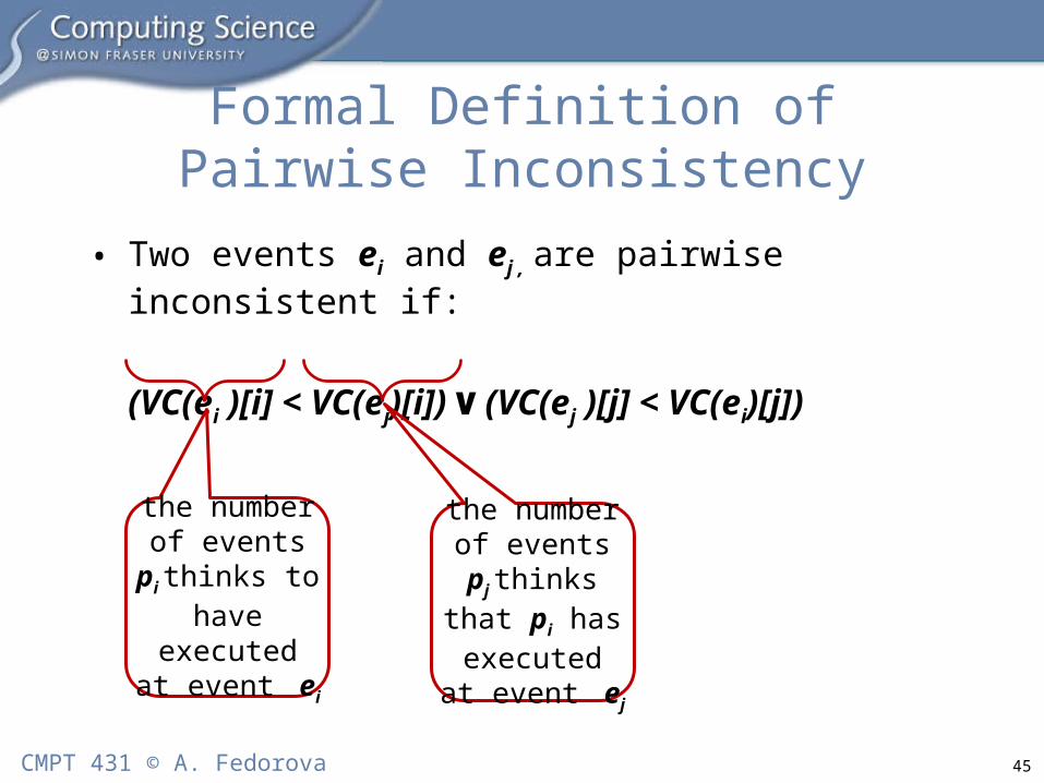
Formal Definition of Pairwise Inconsistency
• Two events ei and ej , are pairwise inconsistent if:
(VC(ei )[i] < VC(ej)[i]) ٧ (VC(ej )[j] < VC(ei)[j])
the number of events pi
thinks to have
executed at event ei
the number of events pj
thinks that pi has
executed at event ej

46CMPT 431 © A. Fedorova
Cut Consistency
• Among all events in the frontier of the cut, check each pair of events for pairwise inconsistency
• If at least two events are pairwise inconsistent, then the cut is inconsistent

47CMPT 431 © A. Fedorova
Is this Cut Consistent?
p1
p2
p3VC[1] = 0VC[2] = 0VC[3] = 1
VC[1] = 1VC[2] = 0VC[3] = 0
VC[1] = 0VC[2] = 1VC[3] = 0
VC[1] = 2VC[2] = 1VC[3] = 0
VC[1] = 1VC[2] = 0VC[3] = 2
VC[1] = 1VC[2] = 0VC[3] = 3
VC[1] = 3VC[2] = 1VC[3] = 3
VC[1] = 1VC[2] = 0VC[3] = 4
VC[1] = 1VC[2] = 2VC[3] = 4
VC[1] = 4VC[2] = 1VC[3] = 3
VC[1] = 4VC[2] = 3VC[3] = 4
VC[1] = 1VC[2] = 0VC[3] = 5
VC[1] = 5VC[2] = 1VC[3] = 3
VC[1] = 5VC[2] = 1VC[3] = 6
VC[1] = 6VC[2] = 1VC[3] = 3

48CMPT 431 © A. Fedorova
And What About This One?
p1
p2
p3VC[1] = 0VC[2] = 0VC[3] = 1
VC[1] = 1VC[2] = 0VC[3] = 0
VC[1] = 0VC[2] = 1VC[3] = 0
VC[1] = 2VC[2] = 1VC[3] = 0
VC[1] = 1VC[2] = 0VC[3] = 2
VC[1] = 1VC[2] = 0VC[3] = 3
VC[1] = 3VC[2] = 1VC[3] = 3
VC[1] = 1VC[2] = 0VC[3] = 4
VC[1] = 1VC[2] = 2VC[3] = 4
VC[1] = 4VC[2] = 1VC[3] = 3
VC[1] = 4VC[2] = 3VC[3] = 4
VC[1] = 1VC[2] = 0VC[3] = 5
VC[1] = 5VC[2] = 1VC[3] = 3
VC[1] = 5VC[2] = 1VC[3] = 6
VC[1] = 6VC[2] = 1VC[3] = 3

49CMPT 431 © A. Fedorova
Active Monitoring
• Recall: we used vector clocks so we can construct consistent global states (or cuts) from processes’ local histories via passive monitoring
• Remember, there is another type of monitoring – active monitoring:– Does not depend of vector clocks, but it is less
powerful• Active monitoring is also referred to as constructing a
distributed snapshot

50CMPT 431 © A. Fedorova
Distributed Snapshot Protocol (Chandy and Lamport)
• Monitor p0 sends “take snapshot” message to all processes pi
• If pi receives such “take snapshot” message for the first time, it:– Records its state– Stops doing any activity related to the distributed computation– Relays the “take snapshot” message on all of its outgoing
channels– Starts recording a state of its incoming channels – records all
messages that have been delivered after the receipt of the first “take snapshot” message

51CMPT 431 © A. Fedorova
Distributed Snapshot Protocol (Chandy and Lamport)(cont.)
• When pi receives a “take snapshot” message for the second time, say from process pj, it stops recording the state of the channel between itself and pj
• When pi receives “take snapshot” message beyond the first one from all processes in a distributed computation, it stops recording the snapshot and sends it to po

52CMPT 431 © A. Fedorova
Properties of Chandy-Lamport Protocol
• Let’s see why this protocol constructs only consistent snapshots, provided that FIFO channels are used
• Recall the key property of a consistent snapshot (i.e., consistent cut):– If event (e → e”) and e” is included in the snapshot,
then e must also be included in that snapshot• Let’s see why this property holds if we use the Chandy-
Lamport distributed snapshot protocol

53CMPT 431 © A. Fedorova
Properties of Chandy-Lamport Protocol
e11
e21
“take snapshot” message
p1
p2
p0
This is the only situation when e21
would be included in the snapshot and e1
1 would not be
Suppose p1 finished taking the snapshot before p2 received the first “take snapshot” message
Let’s see why this won’t happen
snapshot finish
Can it happen that e21 is included in the
snapshot and e11 is not?

54CMPT 431 © A. Fedorova
Properties of Chandy-Lamport Protocol
e11
e21
p1
p2
p0Recall that processes relay the first “take snapshot” message on all outgoing channels
So p1 cannot have finished taking the snapshot before p2 received the first “take snapshot” message.
By protocol, p1 cannot finish the snapshot until it receives the second “take snapshot” message from all other processes
snapshot finish
So that situation will not happen
snapshot finish

55CMPT 431 © A. Fedorova
Using Global States for Evaluating System Properties
• We now know how to construct consistent global states using active and passive monitoring
• Let us look how consistent global states can be used to solve problems in distributed systems
• Global state is constructed in order to evaluate a predicate:– “Is the system in deadlock?”– “Is the memory unreachable (can it be garbage collected)?”– “Does x=y?” (For distributed debugging)

56CMPT 431 © A. Fedorova
Stable and Unstable Predicates
• Predicates can be stable and unstable• A stable predicate does not change its value after the
system has reached this state– Deadlock – once the system deadlocks it stays there– Garbage collection – once the memory is no longer referenced, no
one could acquire a reference for it• An unstable predicate can change its value
– Does x=y? If this were true at one point, it could no longer be true later
• Stable predicates are easy to check – they can be checked from distributed snapshots or vector clock based causal event histories

57CMPT 431 © A. Fedorova
Unstable Predicates Are Harder to Check
e12
e21
p1
p2
VC[1] = 1VC[2] = 0
e11
VC[1] = 0VC[2] = 1
x = 3 x = 4e1
3
e22
y = 6 y = 4
VC[1] = 2VC[2] = 1
VC[1] = 0VC[2] = 2
• Want to evaluate predicate: (y-x) = 2
• An external monitor knows causal ordering of events, not the actual
• Valid actual sequences are:1. e1
1 e21 e1
2 e13 e2
2
2. e11 e2
1 e12 e2
2 e13
• They are both valid because they preserve causal ordering e2
1 → e12
58CMPT 431 © A. Fedorova
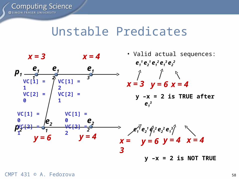
Unstable Predicates
e12
e21
p1
p2
VC[1] = 1VC[2] = 0
e11
VC[1] = 0VC[2] = 1
x = 3 x = 4e1
3
e22
y = 6 y = 4
VC[1] = 2VC[2] = 1
VC[1] = 0VC[2] = 2
• Valid actual sequences:e1
1 e21 e1
2 e13 e2
2
y –x = 2 is TRUE after e13
e11 e2
1 e12 e2
2 e13
y –x = 2 is NOT TRUE
y = 6 x = 4
y = 6 y = 4 x = 4
x = 3
x = 3

59CMPT 431 © A. Fedorova
Detecting “Possibly True”
• With unstable predicates you cannot always detect whether a predicate was definitely true
• But you can detect if it was possibly true• Need to look at all possible valid sequences of events • If the predicate is true in at least one of them, then it is
possibly true• Detecting “possibly true” is useful for distributed
debugging– If a wrong condition is possibly true, the system has a bug– Even if the bug was not triggered it is possible that it will be
triggered under a different ordering of events

60CMPT 431 © A. Fedorova
Detecting “Definitely True”
• Sometimes you can detect definitely true• Construct all valid system states• If the condition is true in all of them, then the condition is
definitely true• Any actual ordering of events would have triggered the
condition, given the correct causal ordering

61CMPT 431 © A. Fedorova
Summary
• Observing a global state of the system is useful for:– Distributed debugging– Distributed garbage collection– Deadlock detection
• Constructing a consistent global state is difficult in absence of global clocks
• Consistent global states can be constructed using– Active monitoring (distributed snapshots)– Passive monitoring (local event histories with vector clock
timestamps)

62CMPT 431 © A. Fedorova
Summary (cont.)
• Distributed snapshots have limited use– Can be used to evaluate stable predicates
• Local event histories with vector clock timestamps contain more information – one can reconstruct a causal history of a distributed computation– Can be used to evaluate unstable predicates
• Unstable predicates cannot always be evaluated with certainty– One can always evaluate “possibly true” – Cannot always evaluate “definitely true”