Embed Size (px)
Citation preview

Coordination, Cooperation, and
Collective Decision
Satoshi Nakada
Submitted in partial fulfillment of the requirements
for the degree of
Doctor of Philosophy
in
Economics
Graduate School of Economics
Hitotsubashi University
2018

c⃝ Copyright 2018
by
Satoshi Nakada

Summary
One of the main goals of modern economics is to understand what mechanism en-
hances self-interested agents’ coordination and cooperation to achieve a good eco-
nomic outcome. This dissertation consists of five essays on studies of this theme. In
the first part, from Chapter 1 to Chapter 3, we consider a problem of how we can
construct an information structure or a mechanism to achieve coordinative outcomes.
In the second part, from Chapter 4 to Chapter 5, we consider desirable allocation
rules of cooperative games and voting rules from normative perspectives.
The first essay studies how risk and ambiguity of each player’s information affect
the possibility of the twin crises, that is, a bank run and a currency crisis simultane-
ously occur. We consider this question by constructing a simple global game model
motivated by Goldstein (2005). In contrast to a standard global game model applied
to the single financial crisis, we assume that two kinds of strategic complementari-
ties exist: (1) strategic complementarity among players within each market and (2)
strategic complementarity among players through the two markets. When each fi-
nancial crisis is considered separately, more ambiguous information triggers the bank
run, whereas less ambiguous information triggers the currency crisis (Ui, 2015). In
contrast to the single financial crisis case, when the two financial markets are linked,
we show that an effect of the additional risk and ambiguity on the possibility of the
crises is not monotone but depends on the degree of a feed-back effect through the
two markets. We characterize all patterns of the effect of the additional risk and am-
biguity on the possibility of the crises. We also characterize an equilibrium outcome
in the limit as the risk and ambiguity vanish.
The second essay studies network games by Jackson and Wolinsky (1996) and
characterizes the class of games that have a network potential. We show that there
exists a network potential if and only if each player’s payoff function can be repre-
sented as the Shapley value of a special class of cooperative games indexed by the
networks. We also show that a network potential coincides with a potential of the
same class of cooperative games.
The third essay studies two-sided one-to-one matching models where we do not
assume either complete nor transitive preferences. In this environment, we cannot

guarantee even the existence of a stable matching, which is one of the fundamen-
tal desiderata for a matching problem. We show that, if each agent’s preference is
acyclic, the DA algorithm with any order extension/completion rule always induces
a stable matching and is strategy-proof. Despite of such good properties, there is no
algorithm in the irrational preference domain such that it is strategy-proof and one-
side optimal when we use an order extension/completion rule. Therefore, our result
clarifies the trade-off between strategy-proofness and one-side optimality beyond the
rational preference domain.
The forth essay studies a new class of allocation rules for cooperative games with
transferable utility (TU-games), weighted egalitarian Shapley values, where each rule
in this class takes into account each player’s contributions and heterogeneity among
players to determine each player’s allocation. We provide an axiomatic foundation for
rules with a given weight profile (i.e, exogenous weights) and the class of rules (i.e.,
endogenous weights). The axiomatization results illustrate the differences among our
class of rules, the Shapley value, the egalitarian Shapley values, and the weighted
Shapley values.
The fifth essay studies normative properties of voting rules. Notably, we propose a
new normative consequentialist criterion for voting rules under Knightian uncertainty
about individuals’ preferences to characterize a weighted majority rule (WMR). This
criterion, which is referred to as robustness, stresses the significance of responsiveness,
i.e., the probability that the social outcome coincides with the realized individual
preferences. A voting rule is said to be robust if, for any probability distribution
of preferences, it avoids the following worst-case scenario: the responsiveness of ev-
ery individual is less than or equal to one-half. Our main result establishes that a
voting rule is robust if and only if it is a WMR without any ties. This characteri-
zation of a WMR avoiding the worst possible outcome complements the well-known
characterization of a WMR achieving the optimal outcome, i.e., efficiency regarding
responsiveness.
ii

Acknowledgments
First of all, I thank my advisor Takashi Ui for his continuous and patient guidance.
Impressed by his studies and sincere attitude for researches, one of the goals of my
Ph.D study has been to write papers that he admits me as an independent researcher.
I hope that this dissertation meets his criteria.
I am also indebted to my dissertation committee members Reiko Goto, Daisuke
Hirata, Koichi Tadenuma, and Norio Takeoka. They gave me fruitful advice that has
significantly improved my works. Their generous support has been also encouraging
me.
Some chapters in my dissertation are collaborated with Takaaki Abe, Shmuel
Nitzan, Kohei Sashida, and Takashi Ui. I appreciate these opportunities. Also, this
dissertation is completed during my visiting at Princeton University. I thank Mark
Fleurbaey for his suggestion and hospitality during this opportunity.
I also have benefited from many people through discussion, interaction, and col-
laborated works. Their encouragement is helpful to my mentality throughout my
whole Ph.D life. I cannot include all of them, but the partial list includes Yukihiko
Funaki, Akifumui Ishihara, Hideshi Itoh, Atsushi Iwasaki, Yusuke Kasuya, Yoshi-
masa Katayama, Takashi Kunimoto, Hitoshi Matsushima, Shintaro Miura, Kota Mu-
rayama, Nozomu Muto, Daisuke Oyama, Hiroyuki Ozaki, Taishi Sassano, Etsuro
Shioji, Yasuhiro Shirata, Takuro Yamashita, and Kazuyoshi Yamamoto.
Finally, I acknowledge the financial support from Japan Society for Promotion of
Science (JSPS).
February, 20, 2018
iii

To my love
iv

Contents
Acknowledgments iii
1 Risk and Ambiguity in the Twin Crises 1
1.1 Introduction . . . . . . . . . . . . . . . . . . . . . . . . . . . . . . . . 1
1.2 Model . . . . . . . . . . . . . . . . . . . . . . . . . . . . . . . . . . . 5
1.2.1 Setup . . . . . . . . . . . . . . . . . . . . . . . . . . . . . . . 5
1.2.2 Knightian uncertainty . . . . . . . . . . . . . . . . . . . . . . 7
1.3 Equilibrium . . . . . . . . . . . . . . . . . . . . . . . . . . . . . . . . 8
1.4 Main results . . . . . . . . . . . . . . . . . . . . . . . . . . . . . . . . 12
1.4.1 Effect of the risk under no-ambiguity . . . . . . . . . . . . . . 12
1.4.2 Effect of the risk and ambiguity . . . . . . . . . . . . . . . . . 13
1.5 Outcomes in the limit case . . . . . . . . . . . . . . . . . . . . . . . . 15
1.6 Conclusion . . . . . . . . . . . . . . . . . . . . . . . . . . . . . . . . . 17
2 A Shapley Value Representation of Network Potentials 19
2.1 Introduction . . . . . . . . . . . . . . . . . . . . . . . . . . . . . . . . 19
2.2 Model . . . . . . . . . . . . . . . . . . . . . . . . . . . . . . . . . . . 21
2.2.1 Setup . . . . . . . . . . . . . . . . . . . . . . . . . . . . . . . 21
2.2.2 Symmetric interaction on networks . . . . . . . . . . . . . . . 23
2.3 Representation theorem . . . . . . . . . . . . . . . . . . . . . . . . . 23
2.3.1 Cooperative games . . . . . . . . . . . . . . . . . . . . . . . . 23
2.3.2 Main results . . . . . . . . . . . . . . . . . . . . . . . . . . . . 25
2.3.3 Relation with other results . . . . . . . . . . . . . . . . . . . . 25
2.4 Examples . . . . . . . . . . . . . . . . . . . . . . . . . . . . . . . . . 30
2.5 Conclusion . . . . . . . . . . . . . . . . . . . . . . . . . . . . . . . . . 33
v

3 Two-sided Matching under Irrational Choice Behavior 34
3.1 Introduction . . . . . . . . . . . . . . . . . . . . . . . . . . . . . . . . 34
3.2 Preliminary . . . . . . . . . . . . . . . . . . . . . . . . . . . . . . . . 37
3.2.1 Model . . . . . . . . . . . . . . . . . . . . . . . . . . . . . . . 37
3.2.2 Stability . . . . . . . . . . . . . . . . . . . . . . . . . . . . . . 38
3.2.3 Motivating examples . . . . . . . . . . . . . . . . . . . . . . . 38
3.3 Main results . . . . . . . . . . . . . . . . . . . . . . . . . . . . . . . . 40
3.3.1 The DA algorithm with completion rules . . . . . . . . . . . . 40
3.3.2 Strategic manipulation . . . . . . . . . . . . . . . . . . . . . . 41
3.3.3 Optimality . . . . . . . . . . . . . . . . . . . . . . . . . . . . . 41
3.4 Conclusion . . . . . . . . . . . . . . . . . . . . . . . . . . . . . . . . . 42
4 The Weighted Egalitarian Shapley Values 44
4.1 Introduction . . . . . . . . . . . . . . . . . . . . . . . . . . . . . . . . 44
4.2 Preliminaries . . . . . . . . . . . . . . . . . . . . . . . . . . . . . . . 47
4.3 Axiomatization of the weighted egalitarian Shapley values . . . . . . 49
4.4 Axiomatization of the weighted egalitarian Shapley values with an ex-
ogenous weight . . . . . . . . . . . . . . . . . . . . . . . . . . . . . . 51
4.5 Conclusion . . . . . . . . . . . . . . . . . . . . . . . . . . . . . . . . . 52
5 Robust Voting under Uncertainty 55
5.1 Introduction . . . . . . . . . . . . . . . . . . . . . . . . . . . . . . . . 55
5.2 Weighted majority rules . . . . . . . . . . . . . . . . . . . . . . . . . 59
5.3 Voting under uncertainty . . . . . . . . . . . . . . . . . . . . . . . . . 60
5.4 Main results . . . . . . . . . . . . . . . . . . . . . . . . . . . . . . . . 63
5.4.1 Characterizations . . . . . . . . . . . . . . . . . . . . . . . . . 63
5.4.2 Proofs . . . . . . . . . . . . . . . . . . . . . . . . . . . . . . . 65
5.5 Robustness vs. efficiency . . . . . . . . . . . . . . . . . . . . . . . . . 67
5.6 Conclusion . . . . . . . . . . . . . . . . . . . . . . . . . . . . . . . . . 70
A Appendix to Chapter 1 72
A.1 Proof of Proposition 1.1 . . . . . . . . . . . . . . . . . . . . . . . . . 72
A.2 Proof of Proposition 1.2 . . . . . . . . . . . . . . . . . . . . . . . . . 76
A.3 Proof of Proposition 1.3 . . . . . . . . . . . . . . . . . . . . . . . . . 76
vi

A.4 Proof of Proposition 1.4 . . . . . . . . . . . . . . . . . . . . . . . . . 77
A.5 Proof of Proposition 1.5 . . . . . . . . . . . . . . . . . . . . . . . . . 78
A.6 Proof of Proposition 1.6 . . . . . . . . . . . . . . . . . . . . . . . . . 79
B Appendix to Chapter 2 81
B.1 Proof of Lemma 2.1 . . . . . . . . . . . . . . . . . . . . . . . . . . . . 81
B.2 Proof of Theorem 2.1 . . . . . . . . . . . . . . . . . . . . . . . . . . . 81
B.3 Proof of Corollary 2.1 . . . . . . . . . . . . . . . . . . . . . . . . . . . 83
B.4 Proof of Corollary 2.2 . . . . . . . . . . . . . . . . . . . . . . . . . . . 84
B.5 Proof of Theorem 2.3 . . . . . . . . . . . . . . . . . . . . . . . . . . . 84
B.6 Additional discussion . . . . . . . . . . . . . . . . . . . . . . . . . . 85
C Appendix to Chapter 3 87
C.1 Proof of Proposition 3.1 . . . . . . . . . . . . . . . . . . . . . . . . . 87
C.2 Proof of Proposition 3.2 . . . . . . . . . . . . . . . . . . . . . . . . . 87
C.3 Proof of Proposition 3.3 . . . . . . . . . . . . . . . . . . . . . . . . . 88
C.4 Proof of Proposition 3.4 . . . . . . . . . . . . . . . . . . . . . . . . . 88
C.5 Relation with Bernheim and Rangel (2009) . . . . . . . . . . . . . . . 89
D Appendix to Chapter 4 92
D.1 Proof of Theorem 4.2 . . . . . . . . . . . . . . . . . . . . . . . . . . . 92
D.2 Independence of axioms for Theorem 4.2 . . . . . . . . . . . . . . . . 95
D.3 A counterexample to Theorem 4.2 and 4.3 for n = 2 . . . . . . . . . . 96
D.4 Proof of Theorem 4.3 . . . . . . . . . . . . . . . . . . . . . . . . . . . 96
D.5 Independence of axioms for Theorem 4.3 . . . . . . . . . . . . . . . . 99
E Appendix to Chapter 5 101
E.1 Other robustness concepts . . . . . . . . . . . . . . . . . . . . . . . . 101
E.2 An imaginary asset market . . . . . . . . . . . . . . . . . . . . . . . . 103
E.3 Robustness vs. optimality . . . . . . . . . . . . . . . . . . . . . . . . 104
E.4 Robustness vs. efficiency: a numerical example . . . . . . . . . . . . . 105
E.5 Proof of Proposition 5.4 . . . . . . . . . . . . . . . . . . . . . . . . . 107
E.5.1 S games . . . . . . . . . . . . . . . . . . . . . . . . . . . . . . 108
E.5.2 Optimal strategies . . . . . . . . . . . . . . . . . . . . . . . . 108
vii

E.5.3 Voting as S game . . . . . . . . . . . . . . . . . . . . . . . . . 109
E.6 Non-robustness of the two-thirds rule . . . . . . . . . . . . . . . . . . 110
References 111
viii
Chapter 1 Risk and Ambiguity in the
Twin Crises
This chapter is based on the same title of the joint work with Kohei Sashida.
1.1 Introduction
A panic-based financial crisis cannot be explained by the underlying fundamental
value alone. In economics, this type of event can be seen as a coordination game in
which such a panic-based crisis is an equilibrium outcome realized from coordination
motives. If two different financial markets are connected, more complicated coordi-
nation motives arise than in the single market case and, as a result, two different
financial crises often occur with a positive correlation. This kind of financial crisis re-
ferred to as twin crises is empirically documented by Kaminsky and Reinhart (1999)
and theoretically studied by Goldstein (2005).1
In the financial market, market participants make decisions based on accessible
information about the underlying fundamental value. Thus, information quality af-
fects what actions are taken by market participants and, in turn, affects the economic
outcome. We usually measure information quality as the precision of information: we
consider a signal with lower variance as the high quality information.2 In contrast
to this view, there is another type of information quality, which is referred to as a
degree of unknown precision of information. As experimental studies suggest, these
two types of information qualities have different implications to a decision maker’s
1The studies of financial crises as coordination games typically face a multiple equilibria problem.To avoid it, incomplete information games which are called global games introduced by Carlsson andvan Damme (1993) are often used. Morris and Shin (2000, 2004) and Goldstein and Pauzner (2005)use a global game to study a bank run problem based on Diamond and Dybvig (1983). Morris andShin (1998) use a global game to study a currency crisis based on Obstfeld (1996). Goldstein (2005)uses a global game to study twin crises. See Morris and Shin (2003) for a survey of the literature.
2Effects of information quality on economic outcomes in this sense are extensively studied. Morrisand Shin (2002) consider how the precision of public and private information affects the social welfarein the beauty contest games. Angeletos and Pavan (2007) and Ui and Yoshizawa (2015) considerthe same question in the more general quadratic payoff games. Iachan and Nenov (2015) considerhow the information quality affects the probability of a financial crisis in the regime change games.
1

2 Chapter 1. Risk and Ambiguity in the Twin Crises
action when a decision maker is ambiguity averse.3 We call the former information
quality as risk and the latter information quality as ambiguity. Ui (2015) shows that
the risk and ambiguity have opposite effects on the possibility of a financial crisis.
In particular, the more ambiguous information triggers the bank run and the less
ambiguous information triggers the currency crisis when we consider these financial
crises separately. In this chapter, we reconsider how the risk and ambiguity affect the
possibility of the financial crises when the two markets are linked.
We answer this question by characterizing how the risk and ambiguity affect the
probability of the twin crises in a simple global game model. Suppose that there
are two financial markets, a commercial banking sector (market B) and a currency
sector (market C). In this economy, an exchange rate is fixed and the government
commits itself to offer financial assistance to the bank to prevent a bank run. Players
of the game are foreign creditors in the market B and speculators in the market C.
In the market B, each creditor can withdraw his own money from the bank in the
short term. In this case, he can obtain no additional dividends. On the other hand,
if he does not withdraw the money from the bank, he may get additional dividends:
the bank invests the amount of money creditors deposit, so if the fundamental of the
economy is good, they can obtain high returns from the investment. However, if many
creditors withdraw the money from the bank, the return will be smaller because the
amount of investment is decreased. In the market C, each speculator wants to attack
the current fixed exchange rate to obtain an arbitrage gain. If he does not attack the
exchange rate, he does not either pay or obtain additional money. On the other hand,
if he attacks the exchange rate and the speculative attack succeeds, he can obtain the
arbitrage gain.
A key point in the model is a strategic feed-back effect through the two markets.
In the market B, the return from the investment by the bank is financed by the
home currency. However, the bank must pay the foreign currency to each creditor.
Therefore, if more speculators attack the exchange rate and, as a result, the value of
the home currency decreases, then the return on the bank also decreases. As a result,
the returns on the creditors decrease as well. Conversely, if more creditors withdraw
their money from the bank, then the government must offer financial assistance to
3The seminal example is Ellsberg (1961). See Gilboa and Marinacci (2013) for a recent survey ofthe literature.

Section 1.1. Introduction 3
the bank. This financial support will cause a downward pressure on the current
exchange rate, which makes the speculative attack successful easier. Therefore, the
more creditors withdraw the money from the bank, the higher payoff speculators can
obtain from the currency attack. Another key point in the model is that we assume
that each player obtains private information about the fundamental of the economy
and he faces ambiguity about the true signal distribution. Our model is a stripped
down version of Goldstein (2005) with an additional assumption that each player
faces ambiguity about the fundamental and is a maximin expected utility decision
maker (Gilboa and Schmeidler, 1989).4
We first show that this model is dominance solvable and has a unique equilibrium.5
The equilibrium is characterized by the cutoff points, that is, each player takes an
action to induce the crises if and only if his signal is less than the cutoff point in
each market. Since we can calculate these cutoff points explicitly, we can provide
comparative statics results of how the risk and ambiguity affect the cutoff points. Our
main result characterizes when the more/less risky and ambiguous information can
reduce the possibility of the crises. The key channel is an influence from one market
to the other market. This power of propagation is captured by what we call attraction
values. We show that if the attraction value of the market B is higher enough than that
of the market C, then the more risky and less ambiguous information can reduce the
possibility of both crises. Conversely, if the attraction value of the market C is higher
enough than that of the market B, then the less risky and more ambiguous information
can reduce the possibility of both crises. In contrast to the single financial crisis case,
these results show that the more ambiguous information may reduce the possibility
of the bank run and the less ambiguous information may reduce the possibility of the
currency crisis depending on the attraction values. Thus, these results have different
implications of the effect of the risk and ambiguity on the possibility of the single
financial crisis from Ui (2015). Summarizing these observations, we show that all
possible patterns of the effect on the possibility of each crisis are classified into twelve
types.
4Laskar (2014) considers a similar linear global game with a maximin expected utility decisionmaker where a single financial market is considered. Our model is an extension of his model toaccommodate a link between the two financial markets.
5Without ambiguity, Goldstein (2005) shows that his model has a unique equilibrium, but hedoes not show that it is survived by the iterative deletion of interim dominated strategies.
4 Chapter 1. Risk and Ambiguity in the Twin Crises
We are also interested in outcomes in the limit as the noise vanishes. The out-
come in the limit can be seen as an approximation of an outcome in the complete
information model. First, we show that two cutoff points have a positive correlation
with each other as demonstrated by Goldstein (2005). In some cases, this correlation
is perfect in the sense that either both crises occur or none of them occurs. Moreover,
the cutoff point in the limit is higher than that of the single market case. Even in
other cases, the cutoff point in the limit in each market is higher than that of the
single market case. A difference from the no-ambiguity case is that relative uncer-
tainty between the risk and ambiguity also affects the prediction of the outcome in
the limit. That is, what limit case we consider depends on the relative convergence
speed of the risk and ambiguity. We show how the outcome in the limit depends on
the relative uncertainty between the risk and ambiguity.
This chapter contributes to the recent growing literature on incomplete informa-
tion games with ambiguity averse players. Epstein (1997) and Epstein and Wang
(1996) consider general incomplete information games with ambiguity averse players
including the maximin decision makers.6 Kajii and Ui (2005) consider the existence
of equilibria and an implication of the strategic ambiguity in the game with the
maximin decision makers. Stauber (2011) considers the robustness of Bayesian Nash
equilibria to small amount of ambiguous information with another type of ambiguity
averse decision makers in the sense of Bewly (2002). Our analysis is consistent with
the framework of Kajii and Ui (2005). Although most papers consider mechanism
designs as applications,7 we consider an impact of the ambiguity on the strategic
situation in global games. In particular, our study complements the finding by Ui
(2015) as an application to the twin crises.8
The rest of this chapter is organized as follows. In section 1.2, we introduce the
model. In section 1.3, we derive the unique equilibrium. In section 1.4, we provide
our main characterization results. In section 1.5, we discuss the outcome in the case
of the small risk and ambiguity. Section 1.6 is the conclusion of this chapter. All
omitted proofs are relegated to Appendix A.
6See also Ahn (2007) and Azrieli and Teper (2011).7See Salo and Weber (1995), Lo (1998), Bose et al. (2006), Turocy (2008), Bose and Daripa
(2009), Bodoh-Creed (2012), Lopomo et al. (2009), Di Tillio et al. (2012), Bose and Renou (2014),and Chiesa et al. (2015).
8Kawagoe and Ui (2015) study a two-player global game experimentally and obtain data sup-porting the finding by Ui (2015).

Section 1.2. Model 5
1.2 Model
1.2.1 Setup
We consider a country where there are two sectors of the financial markets, a banking
sector (market B) and a currency sector (market C). We assume that the exchange
rate is fixed and the government commits itself to offer financial assistance to the
bank to prevent a bank run. In each market, there are continuum of players indexed
by i ∈ [0, 1]. In the market B, each player corresponds to a foreign creditor who
holds claims on the commercial bank in this country. Each player decides whether to
withdraw (W) his money from the bank or not (NW). In the market C, each player
corresponds to a speculator to the fixed exchange rate. Each player decides whether
to attack (A) a fixed exchange rate or not (NA). We denote n ∈ [0, 1] by the fraction
of players who play W in the market B and denote m ∈ [0, 1] by the fraction of players
who play A in the market C. Let θ ∈ R be a common fundamental value in the two
markets.
We then describe each player’s payoff. In the market B, if a player chooses W, he
obtains a constant payoff normalized to 0 regardless of θ and other players’ actions.
On the other hand, if he chooses NW, he obtains αBθ−βBn−γBm where αB, βB, γB >
0. In the market C, if a player chooses NA, he obtains a constant payoff normalized
to 0 regardless of θ and other players’ actions. On the other hand, if he chooses A, he
obtains −αCθ+βCm+γCn where αC , βC , γC > 0. Note that payoffs from W and NA
do not depend on both the state and other players’ actions. We call such an action a
safe action.
In the above payoff specification, the parameters αB and αC correspond to the
marginal payoffs with respect to the fundamental value θ. The parameters βB and
βC are the degrees of strategic complementarity within each market, which describes
marginal payoffs with respect to an increase of n and m, respectively. The key
ingredients of the model are the parameters γB and γC , which are the degrees of
strategic complementarity through the two markets.9 That is, γB describes a degree
of the strategic effect from the market C to the market B and γC describes a degree
of the strategic effect from the market B to the market C.
Each player simultaneously chooses his action in each market. No player can
observe the true value of θ, but each player receives a signal about θ. We assume
9See Goldstein (2005) for a detailed discussion of these parameters.
6 Chapter 1. Risk and Ambiguity in the Twin Crises
that θ is (improperly) uniformly distributed over the real line. Each player i receives
private information xi = θ + εi where εi is independently and identically distributed
according to the normal distribution N(0, σ2). As σ decreases, each agent can obtain
the more precise information about θ. The cumulative distribution function of N(0, 1)
is denoted by Φ(x) : R → [0, 1].
This simple model corresponds to that of Goldstein (2005) in the following sense.
In the market B, each creditor can withdraw his own money from the bank in the
short term. In this case, he can obtain no additional dividends, so that the payoff
is 0. On the other hand, if he does not withdraw the money from the bank, he may
get additional dividends: the bank invests the amount of money creditors deposit,
so if the fundamental of the economy θ is good, they can obtain high returns from
the investment. Therefore, an additional payoff depends on θ and its magnitude is
described by αB. However, if many creditors withdraw the money from the bank,
the return will be smaller because the amount of investment is decreased. This is
the source of the strategic complementarity within the market B and its magnitude
is described by βB.
In the market C, each speculator wants to attack the fixed exchange rate to obtain
an arbitrage gain. If he does not attack the exchange rate, he does not either pay
or obtain additional money, so that the payoff is 0. Conversely, if he attacks the
exchange rate and the speculative attack succeeds, he can obtain the arbitrage gain.
Whether the speculative attack is successful or not depends on the two channels.
The first one is the value of θ: when the fundamental of the economy is bad, the
speculative attack can succeed more easier than when it is good. Therefore, an
additional payoff depends on θ and its magnitude is described by αC . The second
one is the fraction of speculators taking A: the more speculators attack the exchange
rate, the more successful the speculative attack is. This is the source of the strategic
complementarity within the market C and its magnitude is described by βC .
A key ingredient is that there is a strategic feed-back effect through the two
markets. In the market B, the return from the investment by the bank is financed
by the home currency. However, the bank must pay the foreign currency to each
creditor. Therefore, if more speculators attack the exchange rate and, as a result,
the value of the home currency decreases, then the return on the bank also decreases.
As a result, the returns on the creditors decrease as well. This effect is captured by

Section 1.2. Model 7
the parameter γB: when more speculators attack the exchange rate the payoff from
NW decreases. Conversely, if more creditors withdraw their money from the bank,
then the government offers financial assistance to the bank to prevent the bank run.
This financial support will cause a downward pressure on the current exchange rate,
which makes the speculative attack successful easier. Therefore, the more creditors
withdraw the money from the bank, the higher payoff speculators can obtain from the
currency attack. This effect is captured by the parameter γC : when more creditors
withdraw the money from the bank the payoff from A increases.
1.2.2 Knightian uncertainty
We introduce ambiguity about the fundamental to the above setup. In the global
game literature, Laskar (2014) and Ui (2015) consider the effect of ambiguity to the
equilibrium outcome. We follow the model of Laskar (2014) and assume that each
agent receives ambiguous private information as
xi = θ + µi + εi where µi ∈ [−η, η] and η > 0.
Each player knows that µi ∈ [−η, η] but does not know what is the true parameter.
That is, each agent knows that his private information is drawn from the true dis-
tribution in the set{N(µi, σ
2)|µi ∈ [−η, η]}, but does not know what distribution is
true. The parameter η describes the degree of ambiguity: the higher value η takes,
the more ambiguity each player faces. We regard (σ, η) as information quality.
We assume that each player is the maximin decision maker (Gilboa and Schmei-
dler, 1989). Under this hypothesis, each player i is ambiguity averse and evaluates
the payoff from each action in terms of the worst-case scenario over [−η, η] dependingon his private signal xi. Our equilibrium analysis conducted in the next section is
consistent with Kajii and Ui (2005) where they consider an incomplete information
game with the maximin decision makers.10
One might argue why each player faces the ambiguity about the fundamental.
An interpretation is that the policy maker sometimes does not report information
explicitly and sometimes uses ambiguous language strategically, so that the market
participants may interpret the information subjectively.11 Another interpretation is10Lasker (2014) and Ui (2015) can be considered as the specific applications of Kajii and Ui (2007).
Moreover, Ui (2015) considers the more general framework about ambiguous information than thatof Lasker (2014). Hence, Lasker (2014) can be seen as the subclass of Ui (2015).
11See Halpern and Kets (2015) for the discussion of this interpretation.

8 Chapter 1. Risk and Ambiguity in the Twin Crises
that each player considers multiple scenarios based on news. This interpretation may
be relevant when we consider a central bank’s report which is called the fan chart.
Since February 1996, the financial report from the Bank of England has included the
multiple scenarios for the forecast of the inflation rate.12 The fan chart is also used
to forecast other variables like the GDP growth rate and the unemployment rate and
is also used by other central banks like the European Central Bank and the Bank
of Japan. If the market participants are ambiguity averse as in our model, they will
consider the worst-case scenario when they take an action.
1.3 Equilibrium
Following the standard analysis in the global game literature, we focus on monotone
strategies called switching strategies. We show that such a strategy profile constitutes
a unique equilibrium in our model.13 The following calculation is similar to Laskar
(2014).
Let θB and θC be the cutoff values in the market B and C, respectively. The
switching strategies s(θB) and s(θC) are defined as follows.
Market B : si(xi | θB) =
{W if xi ≤ θB,
NW if xi > θB.
Market C : si(xi | θC) =
{A if xi ≤ θC ,
NA if xi > θC .
Following this strategy, each creditor withdraws his money from the bank only
when he obtains a bad signal for the fundamental θ. Similarly, each speculator attacks
the exchange rate only when he obtains a bad signal for the fundamental θ. For each
player i, we denote E[θ | xi] by the conditional expectation of θ on xi. Similarly,
we denote E[n | xi] and E[m | xi] by the conditional expectation of n and m on
xi, respectively. By the law of large numbers and our information structure, we can
calculate each value as follows:
E[θ | xi] = xi − µi.
12See Britton et al. (1998).13Goldstein (2005) shows that the monotone strategy is the only equilibrium strategy under the
no ambiguity case.

Section 1.3. Equilibrium 9
E[n | xi] = Prob(xj ≤ θB | xi)
= Prob(xi − εi − µi + εj + µj ≤ θB | xi)
= Prob(εj − εi ≤ θB − xi + µi − µj | xi)
= Φ(θB − xi√
2σ+µi − µj√
2σ).
E[m | xi] = Prob(xj ≤ θC | xi)
= Prob(xi − εi − µi + εj + µj ≤ θC | xi)
= Prob(εj − εi ≤ θC − xi + µi − µj | xi)
= Φ(θC − xi√
2σ+µi − µj√
2σ).
where we denote j = i by a representative player other than i in view of player i.
We denote πWB (θB, θC , xi, µi, µj) and π
NWB (θB, θC , xi, µi, µj) by the conditional pay-
off on xi of a player in the market B when he takes W and NW, respectively. Similarly,
we denote πAC(θB, θC , xi, µi, µj) and π
NAC (θB, θC , xi, µi, µj) by the conditional payoff on
xi of a player in the market C when he takes A and NA, respectively. By the above
calculation, we obtain the following:
πWB (θB, θC , xi, µi, µj) = 0.
πNWB (θB, θC , xi, µi, µj) = αBE[θ | xi]−βBE[n | xi]−γBE[m | xi]
= αB(xi−µi)−βBΦ(θB−xi√
2σ+µi−µj√
2σ)−γBΦ(
θC−xi√2σ
+µi−µj√
2σ).
πAC(θB, θC , xi, µi, µj) = −αCE[θ | xi] + βCE[m | xi] + γCE[n | xi]
= −αC(xi−µi)+βCΦ(θC−xi√
2σ+µi−µj√
2σ)+γCΦ(
θB−xi√2σ
+µi−µj√
2σ).
πNAC (θB, θC , xi, µi, µj) = 0.
If µi is high, player i can more likely to obtain a good signal, so that the conditional
probability of that other players obtain signals less than the cutoff points is high.
This implies that, in the market B, the expected payoff of i from NW is decreasing
with respect to µi, but in the market C, the expected payoff of i from A is increasing

10 Chapter 1. Risk and Ambiguity in the Twin Crises
with respect to µi. Conversely, if µj is high, player j can more likely to obtain a good
signal, so that the conditional probability (in view of player i) of that player j obtains
a signal less than the cutoff points is low. This implies that, in the market B, the
expected payoff of i from NW is increasing with respect to µj, but in the market C,
the expected payoff of i from A is decreasing with respect to µj. Since each player is
the maximin decision maker, he evaluates the payoff from each action by the values
µi and µj which minimize the expected utility. Therefore, the above arguments imply
that, for players in the market B, they evaluate the expected utility by µi = η and
µj = −η. Similarly, for players in the market C, they evaluate the expected utility by
µi = −η and µj = η. Thus, we have the payoff from each action under the worst-case
scenario as follows:
minµi,µj
πWB (θB, θC , xi, µi, µj) = 0.
VB(xi, (θB, θC)) ≡ minµi,µj
πNWB (θB, θC , xi, µi, µj)
= αB(xi − η)− βBΦ(θB − xi√
2σ+√2η
σ)− γBΦ(
θC − xi√2σ
+√2η
σ).
VC(xi, (θB, θC)) ≡ minµi,µj
πAC(θB, θC , xi, µi, µj)
= −αC(xi + η) + βCΦ(θC − xi√
2σ−√2η
σ) + γCΦ(
θB − xi√2σ
−√2η
σ).
minµi,µj
πNAC (θB, θC , xi, µi, µj) = 0.
Then, we define the functions bB : R2 → {W,NW} and bC : R2 → {A,NA} such
that VB(bB(θB, θC), (θB, θC)) = 0 and VC(bC(θB, θC), (θB, θC)) = 0. Note that, given
θC , (i) VB(xi, (θB, θC)) is continuous with respect to (xi, θB), increasing with respect
to xi, and decreasing with respect to θB, and (ii) VB(k, (k, θC)) is increasing with
respect to k. This implies that the function bB(·, ·) is well-defined. The symmetric
argument shows that bC(·, ·) is also well-defined. By the above argument, if opponents
follow the switching strategies s(θB) and s(θC), the best response for player i is the
switching strategy s(bB(θB, θC)) if i is in the market B and s(bC(θB, θC)) if i is in the
market C. Therefore, if bB(θB, θC) = θB and bB(θB, θC) = θC , the switching strategies

Section 1.3. Equilibrium 11
s(θB) and s(θC) constitute an equilibrium. Thus, we can derive the equilibrium cutoff
points by considering the following simultaneous equations:
αBθB − αBη − βBΦ(√2η
σ)− γBΦ(
θC − θB√2σ
+√2η
σ) = 0, (1.1)
−αCθC − αCη + βCΦ(−√2η
σ) + γCΦ(
θB − θC√2σ
−√2η
σ) = 0. (1.2)
Let θB and θC be the equilibrium cutoff points in the market B and the market
C, respectively. The higher the equilibrium cutoff points become, the easier financial
crises occur. Therefore, we regard θB and θC as the indicators of the probability of
the financial crises.
We can show that these simultaneous equations have the unique solution θB and
θC , which implies the existence of a switching strategy equilibrium. Furthermore, this
is the unique equilibrium and this game is dominance solvable.
Proposition 1.1. The switching strategies s(θB) and s(θC) are the unique strategies
surviving iterated deletion of interim-dominated strategies. In the market B, there
exists the unique cutoff value θB ∈ [θ∗B(σ, η), θ∗∗B (σ, η)] and, in the market C, there
exists the unique cutoff value θC ∈ [θ∗C(σ, η), θ∗∗C (σ, η)] where
θ∗B(σ, σ) = η +βBαB
Φ(√2η
σ),
θ∗∗B (σ, η) =γBαB
+ η +βBαB
Φ(√2η
σ),
θ∗C(σ, η) = −η + βCαC
Φ(−√2η
σ),
θ∗∗C (σ, η) =γCαC
− η +βCαC
Φ(−√2η
σ).
Note that θ∗B and θ∗∗B correspond to the equilibrium cutoff points when players in
the market B believe that m = 0 (θC → −∞) and m = 1 (θC → ∞), respectively.
The former case coincides with the cutoff point where γB = 0 and the latter case
coincides with the cutoff point where every creditor knows every speculator attacks
the exchange rate. A similar argument is also applied for θ∗C and θ∗∗C . By the effect of
the strategic complementarity through the two markets, the equilibrium cutoff points
θB and θC are always higher than θ∗B and θ∗C , respectively. This is an implication of
a strategic feed-back effect through the two markets.14
14Goldstein (2005) calls this feed-back effect as the vicious cycle of the twin crises.

12 Chapter 1. Risk and Ambiguity in the Twin Crises
In contrast to the no-ambiguity case (η = 0), the existence of the ambiguity (η > 0)
has a following effect on the equilibrium cutoff points θB and θC . Since θ∗B(σ, 0) <
θ∗B(σ, η) and θ∗∗B (σ, 0) < θ∗∗B (σ, η), the equilibrium cutoff point θB may increase. On
the contrary, since θ∗C(σ, 0) > θ∗C(σ, η) and θ∗∗C (σ, 0) > θ∗∗C (σ, η), the equilibrium cutoff
point θC may decrease. If γB = γC = 0, this prediction in each market is consistent
with the finding by Ui (2015), who shows that the more ambiguous information
makes each player take a safe action. This means that, in the market B, the more
ambiguous information makes the financial crisis more probable, but, in the market
C, more ambiguous information makes the financial crisis less probable.
However, when γB > 0 and γC > 0, θB may decrease and/or θC may decrease.
This is because the increase of θB may induce the increase of θC and, similarly, the
decrease of θC may induce the decrease of θB by the feed-back effect through the two
markets. In the following section, we characterize how θB and θC are affected by the
increase of σ and η.
1.4 Main results
We consider the effect of the increase of the risk σ and ambiguity η on the equilibrium
cutoff points θB and θC to understand how the probability of the financial crises are
affected by the information quality.
1.4.1 Effect of the risk under no-ambiguity
First, we consider the no-ambiguity case (η = 0) for a comparison. The following
proposition shows that both cutoff points θB and θC are monotonic with respect to
σ.
Proposition 1.2. Let θB =θ∗B+θ∗∗B
2and θC =
θ∗C+θ∗∗C2
. Then, we have the following:
(i) ∂θB∂σ
> 0 if θB ∈ [θ∗B, θB) and∂θB∂σ
≤ 0 if θB ∈ [θB, θ∗∗B ],
(ii) ∂θC∂σ
> 0 if θC ∈ [θ∗C , θC) and∂θC∂σ
≤ 0 if θC ∈ [θC , θ∗∗C ].
Note that Goldstein (2005) does not discuss this kind of comparative statics result
because of the complexity of his model. Intuition behind this result is as follows.
Suppose that θB is sufficiently high (θB > θB). In this case, the region in which
the fundamental θ is less than θB is also large. Therefore, if each player obtains the
more accurate signal, the probability that his private signal is less than the cutoff
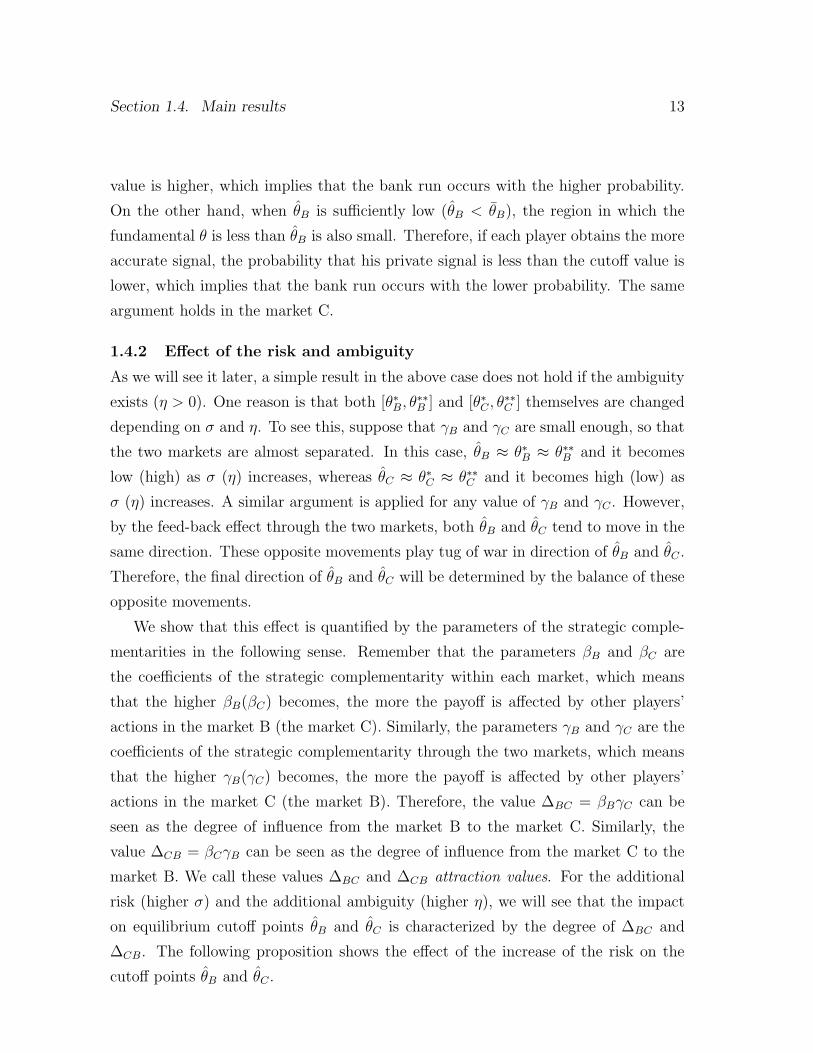
Section 1.4. Main results 13
value is higher, which implies that the bank run occurs with the higher probability.
On the other hand, when θB is sufficiently low (θB < θB), the region in which the
fundamental θ is less than θB is also small. Therefore, if each player obtains the more
accurate signal, the probability that his private signal is less than the cutoff value is
lower, which implies that the bank run occurs with the lower probability. The same
argument holds in the market C.
1.4.2 Effect of the risk and ambiguity
As we will see it later, a simple result in the above case does not hold if the ambiguity
exists (η > 0). One reason is that both [θ∗B, θ∗∗B ] and [θ∗C , θ
∗∗C ] themselves are changed
depending on σ and η. To see this, suppose that γB and γC are small enough, so that
the two markets are almost separated. In this case, θB ≈ θ∗B ≈ θ∗∗B and it becomes
low (high) as σ (η) increases, whereas θC ≈ θ∗C ≈ θ∗∗C and it becomes high (low) as
σ (η) increases. A similar argument is applied for any value of γB and γC . However,
by the feed-back effect through the two markets, both θB and θC tend to move in the
same direction. These opposite movements play tug of war in direction of θB and θC .
Therefore, the final direction of θB and θC will be determined by the balance of these
opposite movements.
We show that this effect is quantified by the parameters of the strategic comple-
mentarities in the following sense. Remember that the parameters βB and βC are
the coefficients of the strategic complementarity within each market, which means
that the higher βB(βC) becomes, the more the payoff is affected by other players’
actions in the market B (the market C). Similarly, the parameters γB and γC are the
coefficients of the strategic complementarity through the two markets, which means
that the higher γB(γC) becomes, the more the payoff is affected by other players’
actions in the market C (the market B). Therefore, the value ∆BC = βBγC can be
seen as the degree of influence from the market B to the market C. Similarly, the
value ∆CB = βCγB can be seen as the degree of influence from the market C to the
market B. We call these values ∆BC and ∆CB attraction values. For the additional
risk (higher σ) and the additional ambiguity (higher η), we will see that the impact
on equilibrium cutoff points θB and θC is characterized by the degree of ∆BC and
∆CB. The following proposition shows the effect of the increase of the risk on the
cutoff points θB and θC .

14 Chapter 1. Risk and Ambiguity in the Twin Crises
Proposition 1.3. There exists values −∞ ≤ Xσ, Yσ ≤ ∞ such that
(i) ∂θB∂σ
< 0 if and only if ∆CB −∆BC < Xσ,
(ii) ∂θC∂σ
< 0 if and only if ∆CB −∆BC < Yσ.
Proposition 1.3 shows that when the effects from the market B to the market C is
high enough, the more risky information can reduce the possibility of each crisis. In
particular, when ∆CB −∆BC < min{Xσ, Yσ}, the more risky information can reduce
the probability of both crises. Similarly, the following proposition shows the effect of
the increase of the ambiguity on the cutoff points θB and θC .
Proposition 1.4. There exists values 0 < Xη and Yη < 0 such that
(i) ∂θB∂η
< 0 if and only if Xη < ∆CB −∆BC ,
(ii) ∂θC∂η
< 0 if and only if Yη < ∆CB −∆BC .
Proposition 1.4 implies that, when γB = γC = 0, ∂θB∂η
> 0 and ∂θC∂η
< 0. This
is consistent with the finding by Ui (2015). However, in general, both ∂θB∂η, ∂θC
∂η< 0
and ∂θB∂η, ∂θC
∂η> 0 will occur depending on the parameters. This is a difference from
the individual finial crisis case, where there is no feed-back effect through the two
markets.
The implications from Proposition 1.3 and 1.4 are as follows. Since critical val-
ues Xσ, Yσ, Xη and Yη are determined by the parameters of the payoff and informa-
tion quality, we can know whether the information disclosure policy with the less
ambiguous and risky information is effective to prevent the financial crises.15 Let
T = ∆CB − ∆BC be the difference of the two attraction values. Depending on the
value of T , we can classify the all possible patterns into twelve types, which are
summarized in Table 1.1.
Goldstein (2005) also discusses some implications focusing on the two points of
policy measures that have a direct effect on the possibility of the one crisis and that
have a direct effect on the possibility of the twin crises. Our results provide a new
insight to the former point. Goldstein (2005) notes that raising the transaction cost
15Effects of additional information on the equilibrium cutoff is also studied by Iachan and Nenov(2015) and Inostroza and Pavan (2017) without ambiguity.
Section 1.5. Outcomes in the limit case 15
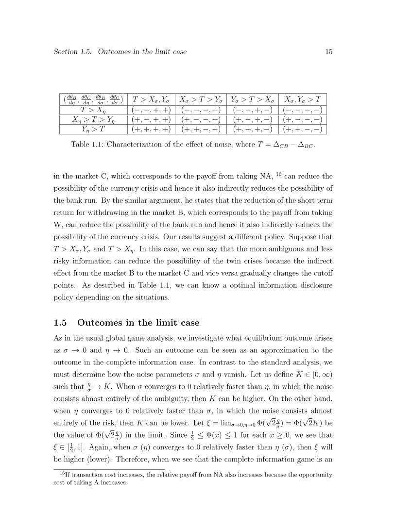
(dθBdη, dθC
dη, dθB
dσ, dθC
dσ) T > Xσ, Yσ Xσ > T > Yσ Yσ > T > Xσ Xσ, Yσ > T
T > Xη (−,−,+,+) (−,−,−,+) (−,−,+,−) (−,−,−,−)Xη > T > Yη (+,−,+,+) (+,−,−,+) (+,−,+,−) (+,−,−,−)
Yη > T (+,+,+,+) (+,+,−,+) (+,+,+,−) (+,+,−,−)
Table 1.1: Characterization of the effect of noise, where T = ∆CB −∆BC .
in the market C, which corresponds to the payoff from taking NA, 16 can reduce the
possibility of the currency crisis and hence it also indirectly reduces the possibility of
the bank run. By the similar argument, he states that the reduction of the short term
return for withdrawing in the market B, which corresponds to the payoff from taking
W, can reduce the possibility of the bank run and hence it also indirectly reduces the
possibility of the currency crisis. Our results suggest a different policy. Suppose that
T > Xσ, Yσ and T > Xη. In this case, we can say that the more ambiguous and less
risky information can reduce the possibility of the twin crises because the indirect
effect from the market B to the market C and vice versa gradually changes the cutoff
points. As described in Table 1.1, we can know a optimal information disclosure
policy depending on the situations.
1.5 Outcomes in the limit case
As in the usual global game analysis, we investigate what equilibrium outcome arises
as σ → 0 and η → 0. Such an outcome can be seen as an approximation to the
outcome in the complete information case. In contrast to the standard analysis, we
must determine how the noise parameters σ and η vanish. Let us define K ∈ [0,∞)
such that ησ→ K. When σ converges to 0 relatively faster than η, in which the noise
consists almost entirely of the ambiguity, then K can be higher. On the other hand,
when η converges to 0 relatively faster than σ, in which the noise consists almost
entirely of the risk, then K can be lower. Let ξ = limσ→0,η→0 Φ(√2 ησ) = Φ(
√2K) be
the value of Φ(√2 ησ) in the limit. Since 1
2≤ Φ(x) ≤ 1 for each x ≥ 0, we see that
ξ ∈ [12, 1]. Again, when σ (η) converges to 0 relatively faster than η (σ), then ξ will
be higher (lower). Therefore, when we see that the complete information game is an
16If transaction cost increases, the relative payoff from NA also increases because the opportunitycost of taking A increases.

16 Chapter 1. Risk and Ambiguity in the Twin Crises
approximation of the incomplete information game where the risk is relatively higher
than the ambiguity, we should consider the outcome in the case of the lower value of
ξ. Similarly, when we see that the complete information game is an approximation
of the incomplete information game where the ambiguity is relatively higher than the
risk, we should consider the outcome in the case of the higher value of ξ. In this sense,
we regard ξ as an indicator of the environment which we want to see approximately.
Note that the limit of θ∗B(σ, η), θ∗∗B (σ, η), θ∗C(σ, η), θ
∗∗C (σ, η) as σ → 0 and η → 0
can be written as follows:
θ∗B(σ, η) → βBαB
ξ (σ → 0, η → 0),
θ∗∗B (σ, η) → γBαB
+βBαB
ξ (σ → 0, η → 0),
θ∗C(σ, η) → βCαC
− βCαC
ξ (σ → 0, η → 0),
θ∗∗C (σ, η) → γCαC
+βCαC
− βCαC
ξ (σ → 0, η → 0).
Let us denote θ∗B(ξ) = βB
αBξ, θ∗∗B (ξ) = γB
αB+ βB
αBξ, θ∗C(ξ) = βC
αC− βC
αCξ, θ∗∗C (ξ) =
γCαC
+ βC
αC− βC
αCξ by each value in the limit. Depending on the parameters, the re-
gions [θ∗B(ξ), θ∗∗B (ξ)] and [θ∗C(ξ), θ
∗∗C (ξ)] may overlap with each other or there is no
intersection. The possible patterns are as follows:
(i) θ∗B(ξ) < θ∗C(ξ) < θ∗∗B (ξ) < θ∗∗C (ξ),
θ∗B(ξ) < θ∗C(ξ) < θ∗∗C (ξ) < θ∗∗B (ξ),
θ∗C(ξ) < θ∗B(ξ) < θ∗∗C (ξ) < θ∗∗B (ξ),
θ∗C(ξ) < θ∗B(ξ) < θ∗∗B (ξ) < θ∗∗C (ξ).
(ii) θ∗B(ξ) < θ∗∗B (ξ) < θ∗C(ξ) < θ∗∗C (ξ).
(iii) θ∗C(ξ) < θ∗∗C (ξ) < θ∗B(ξ) < θ∗∗B (ξ).
Depending on each case, we obtain the following result, which corresponds to
Proposition 2 of Goldstein (2005).
Section 1.6. Conclusion 17
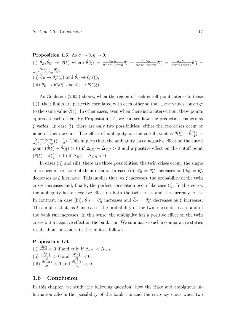
Proposition 1.5. As σ → 0, η → 0,
(i) θB, θC → θ(ξ) where θ(ξ) = αBγCαBγC+αCγB
θ∗B + αCγBαBγC+αCγB
θ∗∗C = αBγCαBγC+αCγB
θ∗∗B +αCγB
αBγC+αCγBθ∗C ,
(ii) θB → θ∗∗B (ξ) and θC → θ∗C(ξ),
(iii) θB → θ∗B(ξ) and θC → θ∗∗C (ξ).
As Goldstein (2005) shows, when the region of each cutoff point intersects (case
(i)), their limits are perfectly correlated with each other so that these values converge
to the same value θ(ξ). In other cases, even when there is no intersection, these points
approach each other. By Proposition 1.5, we can see how the prediction changes as
ξ varies. In case (i), there are only two possibilities: either the two crises occur or
none of them occurs. The effect of ambiguity on the cutoff point is θ(ξ) − θ(12) =
∆BC−∆CB
αBγC+αCγB(ξ− 1
2). This implies that, the ambiguity has a negative effect on the cutoff
point (θ(ξ) − θ(12) > 0) if ∆BC − ∆CB > 0 and a positive effect on the cutoff point
(θ(ξ)− θ(12) < 0) if ∆BC −∆CB < 0.
In cases (ii) and (iii), there are three possibilities: the twin crises occur, the single
crisis occurs, or none of them occurs. In case (ii), θB = θ∗∗B increases and θC = θ∗C
decreases as ξ increases. This implies that, as ξ increases, the probability of the twin
crises increases and, finally, the perfect correlation occur like case (i). In this sense,
the ambiguity has a negative effect on both the twin crises and the currency crisis.
In contrast, in case (iii), θB = θ∗B increases and θC = θ∗∗C decreases as ξ increases.
This implies that, as ξ increases, the probability of the twin crises decreases and of
the bank run increases. In this sense, the ambiguity has a positive effect on the twin
crises but a negative effect on the bank run. We summarize such a comparative statics
result about outcomes in the limit as follows.
Proposition 1.6.
(i) dθ(ξ)dξ
< 0 if and only if ∆BC < ∆CB,
(ii)dθ∗∗B (ξ)
dξ> 0 and
dθ∗C(ξ)
dξ< 0,
(iii)dθ∗B(ξ)
dξ> 0 and
dθ∗∗C (ξ)
dξ< 0.
1.6 Conclusion
In this chapter, we study the following question: how the risky and ambiguous in-
formation affects the possibility of the bank run and the currency crisis when two

18 Chapter 1. Risk and Ambiguity in the Twin Crises
financial markets are linked. We construct a simple global game model inspired by
Goldstein (2005) and show that the effect of noise on the possibility of the financial
crises can be different from the single financial crisis by Ui (2015). Our characteri-
zation of the effect of the risk and ambiguity on the possibility of the financial crises
has some implications about an information disclosure policy to prevent the crises.

Chapter 2 A Shapley Value
Representation of Network
Potentials
2.1 Introduction
A network game is introduced by Jackson and Wolinsky (1996) to study what net-
works emerge through self-interested agents’ strategic interaction.1 One of the solu-
tion concepts in network games is pairwise stability defined by Jackson and Wolinsky
(1996). A network is pairwise stable if there is neither a player who prefers to sever a
current link with his neighbor nor a pair of players who prefer to make a new link. It is
known that a pairwise stable network exists if there exists a network potential (Jack-
son, 2003; Chakrabarti and Gilles, 2007), which can be considered as an imaginary
representative player’s payoff function.
A network potential is closely related to the Shapley value. Jackson (2003) shows
that if each player’s payoff function can be represented as the Shapley value of a
network value function, which assigns a collective payoff generated by players to each
network, then a network game admits a network potential, but it has been an open
question whether or not the converse is also true.2 On the other hand, Chakrabarti
and Gilles (2007), who formally define a network potential, show that a network
potential exists if a network payoff function satisfies the property called the Shapley
value consistency, while they also demonstrate that its converse is not true: it is only
a sufficient condition for the existence of the network potential.
This chapter provides a necessary and sufficient condition for the existence of
network potentials in terms of the Shapley value and clarify the relationship between
network potentials and the Shapley value. To this end, we introduce a collection
of characteristic functions indexed by networks such that a collective payoff to a
1Examples include supply chain networks among firms (Palsule-Desai et al., 2013), FTAs amongseveral countries (Goyal and Joshi, 2006; Furusawa and Konishi, 2007), and social network services(Farrell and Fudge, 2013). See Jackson (2008) for other examples.
2Jackson (2003) does not give the formal definition of network potentials.
19

20 Chapter 2. A Shapley Value Representation of Network Potentials
coalition is determined by the sub-graph restricted to the coalition. We call it a
network characteristic function, which has more degree of freedom than that of a
network value function. More specifically, a value function is a function which assigns
a real number to each network, whereas a network characteristic function is a function
which assigns a real number to each pair of network and coalition. In this sense, it
generalizes a network value function; that is, for any network value function, there
exists a network characteristic function that represents the network value function,
but not vice versa.
Our main result shows that there exists a network potential if and only if each
player’s payoff function can be represented as the Shapley value of a network char-
acteristic function. This result is shown by the following three steps. First, we show
that there exists a network potential if and only if each player’s payoff function can be
represented as an interaction network potential, which is a collection of functions in-
dexed by coalitions such that each function assigns a collective payoff to each network
restricted to the coalition. Second, we show that there is a one-to-one correspondence
between an interaction network potential and a network characteristic function in the
sense that a collection of the Mobius inverses of the characteristic functions corre-
sponds to the interaction network potential. Finally, since the Shapley value of each
characteristic function can be represented as the sum of its Mobius inverses proved
by Shapley (1953), the above argument shows that the condition for the existence of
a network potential is equivalent to the condition that each player’s payoff function
can be represented as the Shapley value of a network characteristic function. The ar-
gument of the proof is an application of Ui (2000) to network games, who shows that
there exists a potential of noncooperative games by Monderer and Shapley (1996)
if and only if each player’s payoff function is represented as the Shapley value of a
particular class of cooperative games indexed by strategy profiles.
Our result generalizes the result of Jackson (2003). As we mentioned above,
Jackson (2003) shows that if each player’s payoff function can be represented as the
Shapley value of a network value function, then a network game admits a network
potential. Because a network value function is a special case of a network charac-
teristic function, our result provides an alternative proof for that of Jackson (2003).
Moreover, we can show that the converse of Jackson (2003)’s result is not true by con-
structing a network characteristic function that cannot be represented as a network

Section 2.2. Model 21
value function.
Our result also generalizes the result of Chakrabarti and Gilles (2007). As we
mentioned above, Chakrabarti and Gilles (2007) show that a network potential exists
if a network payoff function satisfies the property called the Shapley value consistency.
If each player’s payoff function satisfies the Shapley value consistency, we can show
that it can be represented as the Shapley value of a network characteristic function.
Therefore, our result also provides an alternative proof for that of Chakrabarti and
Gilles (2007).
Except for our result, there is another characterization result for the existence of
a network potential by Chakrabarti and Gilles (2007) in terms of potential games.
Chakrabarti and Gilles (2007) show that a network potential exists if and only if the
corresponding game, called Myerson’s consent game (Myerson, 1991), is a potential
game.3 A drawback of this result is that it requires an indirect step to identify the
existence of a network potential; that is, we need additional results to check whether
the corresponding game is a potential game or not. In contrast, we provide a direct
condition to identify the existence of a network potential. Moreover, combining the
result of Ui (2000) with ours, we can derive the characterization of Chakrabarti and
Gilles (2007) as a byproduct and show the coincidence of potentials in the different
class of games: network games, noncooperative games, and cooperative games.
The rest of this chapter is organized as follows. In section 2.2, we define a formal
model. In section 2.3, we show our main results. In section 2.4, we discuss some
examples to show how our results are useful to find a network potential. Section 2.5
concludes the chapter. Omitted proofs are relegated to Appendix B.
2.2 Model
2.2.1 Setup
Let N = {1, · · · , n} be a (finite) set of players. A network is described by an undi-
rected graph whose nodes are players. Let gN = {ij|i, j ∈ N, i = j} be a set of
all possible links. Then, a network g is a subset of gN . We denote the set of all
networks by GN = {g|g ⊂ gN}. For each network g ∈ GN and player i ∈ N , let
3Myerson’s consent game is a network formation game such that each player’s action is to choosethe set of other players with whom he wants to make links and each player’s payoff function dependsupon the constructed network. See Section 2.3 for the formal definition and discussion.

22 Chapter 2. A Shapley Value Representation of Network Potentials
Ni(g) = {j ∈ N |i = j and ij ∈ g} be the set of i’s neighborhood in g. For each
S ∈ 2N and g ∈ GN , let g|S = {ij ∈ g|i ∈ S and j ∈ S} be a restricted network
whose nodes are in S. We denote by GS the set of networks where the set of players is
S. For each ij ∈ g, let g − ij = g\{ij} be the network which remains after removing
a link ij from g. Similarly, for each ij /∈ g, let g + ij = g ∪ {ij} be the network
formed by adding a link ij to g. The payoff function for player i ∈ N is denoted by
ϕi : GN → R. Jackson and Wolinsky (1996) call ϕ = (ϕi)i∈N a network game.
A solution concept on network games is pairwise stability defined by Jackson and
Wolinsky (1996). A network is pairwise stable if there is neither a player who wants
to sever the link with his neighbor nor a pair of players who agree to make a new
link.
Definition 2.1. A network g is pairwise stable if
(i) for all ij ∈ g, ϕi(g) ≥ ϕi(g − ij) and ϕj(g) ≥ ϕj(g − ij), and
(ii) for all ij /∈ g, if ϕi(g) < ϕi(g + ij) then ϕj(g) > ϕj(g + ij).
A sufficient condition for the existence of a pairwise stable network is the existence
of a network potential function defined by Chakrabarti and Gilles (2007). The func-
tion is analogous to the potential function defined by Monderer and Shapley (1996)
in noncooperative games.
Definition 2.2. A network game ϕ = (ϕi)i∈N admits a network potential if there is
a function ω : GN → R such that, for any g ∈ GN and ij ∈ g,
ϕi(g)− ϕi(g − ij) = ω(g)− ω(g − ij).
If a network game ϕ admits a network potential function ω, it is known that its
maximizers are pairwise stable networks. Since there are a finite number of networks,
a maximizer of ω always exists, which implies the existence of a pairwise stable
network. The following result summarizes this observation.
Proposition 2.1. Suppose that a network game ϕ = (ϕi)i∈N admits a network po-
tential function ω. Then, there is at least one pairwise stable network. Moreover, a
maximizer of ω is a pairwise stable network.

Section 2.3. Representation theorem 23
2.2.2 Symmetric interaction on networks
To illustrate how to find a network potential, consider the following network game.
Let N = {1, 2, 3} be the set of players. We assume that payoff functions are as follows:
for each S ∈ 2N , there exists a function wS : GS → R such that
ϕi(g) = w{i}(∅) +∑j =i
w{i,j}(g|{i,j}) + wN(g).
We call ϕ a symmetric interaction network game (SI network game) in the sense
that each player’s payoff function is described by symmetric bilateral interaction terms
and a total interaction term.
Let us define the function ω : GN → R such that
ω(g) =∑i∈N
w{i}(∅) +∑i<j
w{i,j}(g|{i,j}) + wN(g).
Then, for each i, j ∈ N with ij ∈ g,
ϕi(g)− ϕi(g − ij) = (w{i,j}(g|{i,j})− w{i,j}((g − ij)|{i,j}))) + (wN(g)− wN(g − ij))
= ω(g)− ω(g − ij).
Therefore, a SI network game admits a network potential function. We will show
that a condition of the existence of a network potential function is equivalent to the
condition that each player’s payoff function ϕi can be decomposed into symmetric
interaction terms such as a SI network game.
2.3 Representation theorem
2.3.1 Cooperative games
To state our results, we prepare some concepts of cooperative games. A characteristic
function or a TU game is defined as a function v : 2N → R such that v(∅) = 0. We
denote the set of all TU games by GN .
For each T ∈ 2N , a unanimity game uT ∈ GN is defined as
uT (S) =
{1 if T ⊂ S,
0 otherwise.
24 Chapter 2. A Shapley Value Representation of Network Potentials
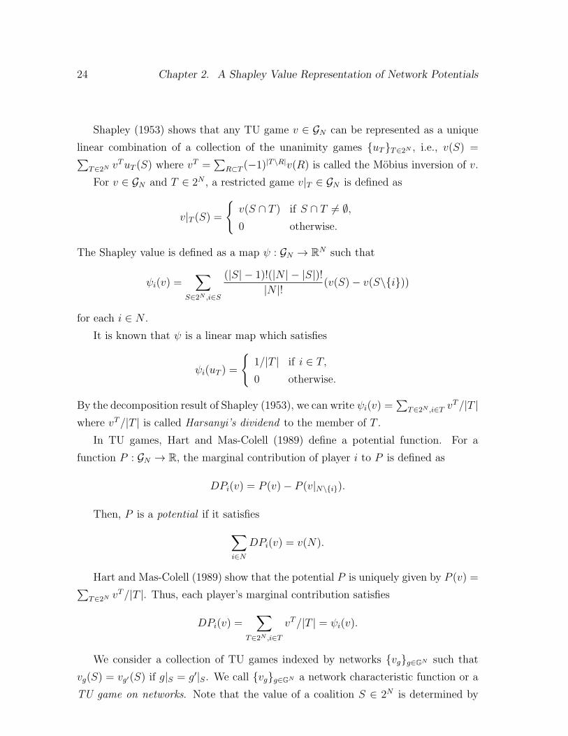
Shapley (1953) shows that any TU game v ∈ GN can be represented as a unique
linear combination of a collection of the unanimity games {uT}T∈2N , i.e., v(S) =∑T∈2N v
TuT (S) where vT =
∑R⊂T (−1)|T\R|v(R) is called the Mobius inversion of v.
For v ∈ GN and T ∈ 2N , a restricted game v|T ∈ GN is defined as
v|T (S) =
{v(S ∩ T ) if S ∩ T = ∅,0 otherwise.
The Shapley value is defined as a map ψ : GN → RN such that
ψi(v) =∑
S∈2N ,i∈S
(|S| − 1)!(|N | − |S|)!|N |!
(v(S)− v(S\{i}))
for each i ∈ N .
It is known that ψ is a linear map which satisfies
ψi(uT ) =
{1/|T | if i ∈ T,
0 otherwise.
By the decomposition result of Shapley (1953), we can write ψi(v) =∑
T∈2N ,i∈T vT/|T |
where vT/|T | is called Harsanyi’s dividend to the member of T .
In TU games, Hart and Mas-Colell (1989) define a potential function. For a
function P : GN → R, the marginal contribution of player i to P is defined as
DPi(v) = P (v)− P (v|N\{i}).
Then, P is a potential if it satisfies∑i∈N
DPi(v) = v(N).
Hart and Mas-Colell (1989) show that the potential P is uniquely given by P (v) =∑T∈2N v
T/|T |. Thus, each player’s marginal contribution satisfies
DPi(v) =∑
T∈2N ,i∈T
vT/|T | = ψi(v).
We consider a collection of TU games indexed by networks {vg}g∈GN such that
vg(S) = vg′(S) if g|S = g′|S. We call {vg}g∈GN a network characteristic function or a
TU game on networks. Note that the value of a coalition S ∈ 2N is determined by

Section 2.3. Representation theorem 25
the network structure in S and not by the network structure of N\S. We denote by
GN,GN = {{vg}g∈GN |vg(S) = vg′(S) if g|S = g′|S} the set of all TU games on networks.
The following lemma shows a property of Harsanyi’s dividends of {vg}g∈GN .
Lemma 2.1. {vg}g∈GN ∈ GN,GN if and only if g|S = g′|S implies vSg = vSg′ for any
S ∈ 2N .
2.3.2 Main results
The goal of this section is to show a relationship between network potentials and
the Shapley value. Let us consider a collection of functions {ζS}S∈2N such that ζS :
GS → R. We call a collection of functions an interaction network potential, which
is analogous to the definition of an interaction potential defined by Ui (2000). Our
main result is the following representation theorem.
Theorem 2.1. For any network game ϕ = (ϕi)i∈N , the following statements are
equivalent:
(i) The network game ϕ admits a network potential.
(ii) There exists a TU game on networks {vg}g∈GN ∈ GN,GN such that
ϕi(g) = ψi(vg) for all i ∈ N.
(iii) There exists an interaction network potential {ζS}S∈2N such that
ϕi(g) =∑
S∈2N ,i∈S
ζS(g|S) for all i ∈ N.
Furthermore, a network potential function ω is given by
ω(g) = P (vg) =∑S∈2N
ζS(g|S).
Theorem 2.1 shows that a SI network game in the three player case in section 2.2
is a special case of the network games which have a network potential. A family of
the functions wS : GS → R for each S ∈ 2N is an interaction network potential.
2.3.3 Relation with other results
In this subsection, we discuss the relation between our results and previous results by
Jackson (2003) and Chakrabarti and Gilles (2007). Jackson (2003) and Chakrabarti
and Gilles (2007) show a sufficient condition for the existence of network potentials.
26 Chapter 2. A Shapley Value Representation of Network Potentials
We show that both of results are corollaries of Theorem 2.1. Moreover, we provide
an alternative simple proof of a characterization result of the existence of network
potentials by Chakrabarti and Gilles (2007) in terms of potential games.
Myerson-Jackson-Wolinsky value. Jackson and Wolinsky (1996) consider the
following network game. Let v : GN → R be a network value function. We denote
by GN the set of all network value functions. Unlike a TU-game, the value of v
depends on the networks rather than coalitions. We say that v is component additive
if∑
h∈C(g) v(h) = v(g) where C(g) is the set of a connected components of g. Let
Π(g) ⊂ 2N be the set of coalitions such that each player is connected in g. A mapping
f : GN ×GN → RN is called an allocation rule. Jackson and Wolinsky (1996) define
the allocation rule, which we call the Myerson-Jackson-Wolinsky value, such that, for
each i ∈ N ,
fMJWi (v, g) =
∑S⊂N\{i}
|S|!(|N | − |S| − 1)!
|N |!(v(g|S∪{i})− v(g|S)).
Like Myerson (1977), Jackson and Wolinsky (1996) show that fMJW (v, g) is the
unique allocation rule satisfying following properties.
Component balance (CB): for any component additive v, g ∈ GN , and S ∈ Π(g),∑i∈S fi(v, g) = v(g|S).
Equal bargaining power (EBP): for any component additive v, for any g ∈ GN
and any ij ∈ g, fi(v, g)− fi(v, g − ij) = fj(v, g)− fj(v, g − ij).
In this setup, Jackson (2003) shows the following result, which is implied by
Theorem 2.1.
Corollary 2.1. (Proposition 2 of Jackson, 2003). Suppose that a network game
ϕ = (ϕi)i∈N satisfies ϕi(g) = fMJWi (v, g) for some v ∈ GN . Then, a network game ϕ
admits a network potential ω(g) =∑
S⊂N(|S|−1)!(|N |−|S|)!
|N |! (v(g|S)).
This result states that network games where each player’s payoff function is given
by fMJWi (v, g) admit network potentials. A key idea behind Corollary 2.1 is that,

Section 2.3. Representation theorem 27
for each network value function v, there is a network characteristic function {vg}g∈GN
such that vg(S) = v(g|S) for all S ∈ 2N and g ∈ GN . However, the converse of the
result is not true in general. To see this, consider the following network game. Each
player’s payoff function is given in Table 2.1.
Network ϕ1(g) ϕ2(g) ϕ3(g) ω(g)g0 = ∅ 0 0 0 0g1 = {12} 5/6 5/6 2/6 5/6g2 = {13} 1 0 1 1g3 = {23} −1 9/6 9/6 9/6g4 = {12, 13} 11/6 5/6 8/6 11/6g5 = {12, 23} 7/6 22/6 19/6 22/6g6 = {13, 23} −2/6 7/6 13/6 13/6g7 = gN 13/6 22/6 25/6 28/6
Table 2.1: Payoff functions of the network game.
Note that this game admits a network potential function ω. By Theorem 2.1, there
is a TU game on networks {vg}g∈GN such that ϕi(g) = ψi(vg). By efficiency of the
Shapley value, vg(N) must satisfy the following: vg0(N) = 0, vg1(N) = 2, vg2(N) =
2, vg3(N) = 2, vg4(N) = 4, vg5(N) = 8, vg6(N) = 3, vg7(N) = 10.4 An example of
{vg}g∈GN is given in Table 2.2.
vg\S {1} {2} {3} {1, 2} {1, 3} {2, 3} Nvg0 0 0 0 0 0 0 0vg1 0 0 0 1 0 0 2vg2 0 0 0 0 2 0 2vg3 0 0 0 0 0 5 2vg4 0 0 0 1 2 0 4vg5 0 0 0 1 0 5 8vg6 0 0 0 0 2 5 3vg7 0 0 0 1 2 5 10
Table 2.2: An example of {vg}g∈GN such that ϕi(g) = ψi(vg).
If there is a network value function v which satisfies ϕi(g) = fMJWi (v, g), then
4Shapley value satisfies the efficiency such that∑
i∈N ψi(v) = v(N) for all v ∈ GN .

28 Chapter 2. A Shapley Value Representation of Network Potentials
v(g) = v(g|N) = vg(N) = vg(N) because fMJWi (v, g) = ψi(vg) and the efficiency
of ψi(vg). However, if it is true, we have fMJW1 (v, g1) = fMJW
1 (v, g1) = 1 and
fMJW3 (v, g1) = 0 because
v(g1|S) =
{2 if S = {1, 2} or N,
0 otherwise.
Therefore, there is no value function v which satisfies ϕi(g) = fMJWi (v, g) although
this game admits a network potential.
A reason behind this observation is that the number of degrees of freedom for a
value function is smaller than that of a network characteristic function because the
former is a function from GN to R, whereas the latter is a function from GN × 2N to
R.
Shapley value consistency. For a network game ϕ, Chakrabarti and Gilles (2007)
consider the following TU game: for each g ∈ GN , let us define Uϕ,g : 2N → R such
that
Uϕ,g(S) =∑i∈S
ϕi(g|S)
for all S ∈ 2N .
We say that a network game ϕ is Shapley value consistent if for every g ∈ GN , it
holds that ϕi(g) = ψi(Uϕ,g). They show the following result, which is also implied by
Theorem 2.1.
Corollary 2.2. (Theorem 3.7 of Chakrabarti and Gilles, 2007). If a network game
ϕ is Shapley value consistent, then a network game ϕ admits a network potential.
Chakrabarti and Gilles (2007) show an example where a network potential exists
although ϕ is not Shapley value consistent.5 If ϕ is Shapley value consistent, then the
family of games {Uϕ,g}g∈GN is a TU game on networks. However, for the existence of
a network potential, Theorem 2.1 says that we need TU games on networks, which is
not necessary Shapley value consistent.
5See Appendix B.6 for the formal argument. In the example, we demonstrate that there is anetwork characteristic function {vg}g∈GN which satisfies the condition of Theorem 2.1, whereas thenetwork game is not Shapley value consistent.

Section 2.3. Representation theorem 29
Potential games. For each i ∈ N , let Ai be the set of strategies and ui : A→ R be
the payoff function where A = A1 × · · · × An. We denote (N,A, u) a strategic form
game. Monderer and Shapley (1996) define the class of potential games.
Definition 2.3. A game (N,A, u) is called a potential game if there is a function
V : A→ R such that, for each i ∈ N, a′i ∈ Ai and a ∈ A,
ui(a′i, a−i)− ui(a) = V (a′i, a−i)− V (a).
Let us consider a collection of TU games {va}a∈A such that va(S) = v′a(S) if
aS = a′S, which is called a TU game with action choices. We denote by GN,A =
{{va}a∈A|va(S) = v′a(S) if aS = a′S} the set of all TU games with action choices.
Ui (2000) shows the following relationship between potential games and the Shapley
value, and hence the potential of a TU game.
Theorem 2.2. (Theorem 2 of Ui, 2000). For any game (N,A, u), the following
statements are equivalent:
(i) (N,A, u) is a potential game.
(ii) There exists a TU game with action choices {va}a∈A ∈ GN,A such that
ui(a) = ψi(va) for all i ∈ N .
Furthermore, a potential function V is given by
V (a) = P (va).
We consider the following network formation game by Myerson (1991) to state
another characterization result of the existence of a network potential in terms of
potential games by Chakrabarti and Gilles (2007). This game is called a consent
game. Given a network game ϕ = (ϕi)i∈N , let Ai = {(lij)j =i|lij ∈ {0, 1}} be the
set of actions for player i. We denote by li = (lij)j =i a typical element of Ai. Let
σ(l) = {ij ∈ gN |lij ·lji = 1} be an network induced by the action profile l = (li)i∈N . We
call (N,A, πϕ) a consent game corresponding a network game ϕ if πϕ,i(l) = ϕi(σ(l)).
Let Ag = {l ∈ A|σ(l) = g} be the set of strategy profiles which induce the network g.
Note that each strategy profile l induces the unique network σ(l), but there are many
strategy profiles which induce the same network. We define lg ∈ Ag as the (unique)

30 Chapter 2. A Shapley Value Representation of Network Potentials
non-superfluous strategy profile such that, for all pair i, j ∈ N , lg,ij = 1 if and only
if ij ∈ g. Chakrabarti and Gilles (2007) show the following characterization result.
By using Theorem 2.1 and 2.2, we can provide much simpler proof than the original
proof.
Theorem 2.3. (Theorem 3.3 of Chakrabarti and Gilles, 2007). A network game
ϕ = (ϕi)i∈N admits a network potential if and only if the corresponding consent game
(N,A, πϕ) is a potential game.
According to this result, we have to consider whether the corresponding consent
game is a potential game or not to check the existence of a network potential. In
contrast, Theorem 2.1 can be directly applied to the underlying network game ϕ.
Combing Theorem 2.1, 2.2 and 2.3, we can say the following unified relationship
among potential functions of different types of games: network games, cooperative
games, and noncooperative games.
Corollary 2.3. A network game ϕ admits a network potential ω(·) if and only if there
exists a TU game on networks {vg}g∈GN ∈ GN,GN such that ω(g) = P (vg) = V (lg)
where V (·) is a potential function of the corresponding consent game (N,A, πϕ).
2.4 Examples
In this section, we consider the following examples to demonstrate the applicability
of theorem 2.1 to find a network potential. For each network g ∈ GN and for each
distinct i, j ∈ N , let
gij =
{1 if ij ∈ g,
0 otherwise.
Example 2.1 (Social distance (Iijima and Kamada, 2016).6 Suppose that each player
i has a multidimensional (m-dimension) characteristic, which is called type, xi =
(xi1, · · · , xim) ∈ [0, 1]m. Let d : X×X → R represent a metric, called social distance,
which measures the relation/similarity among players. They assume that each player’s
payoff function is as follows:
ϕi(g) =
∑j∈Ni(g)
b(d(xi, xj))
− c(qi),
6We thank Ryota Iijima for suggesting this model.
Section 2.4. Examples 31
where b(·) > 0 is a weakly decreasing, left-continuous function, and qi = |Ni(g)|.Assume that c(·) is linear i.e., c(qi) = cqi for some constant c > 0.7
Let us define
ζS(g|S) =
{(b(d(xi, xj))− c)gij if S = {i, j},0 otherwise.
Then, an interaction network potential {ζS}S∈2N satisfies
ϕi(g) =∑
S∈2N ,i∈S
ζS(g|S)
for all i ∈ N .
Thus, by Theorem 2.1, this network game ϕ admits a network potential and it is
given by
ω(g) =∑i<j
(b(d(xi, xj))− c)gij =1
2
∑i∈N
ϕi(g).
By Proposition 2.1, a pairwise stable network exists. Moreover, for a network
g /∈ argmaxg′∈GNw(g′), (i) there is a pair ij ∈ g such that b(d(xi, xj)) < c or (ii)
there is a pair ij /∈ g such that b(d(xi, xj)) > c, which implies that g is not pair-
wise stable. Therefore, g is pairwise stable if and only if g ∈ argmaxg′∈GNw(g′) =
argmaxg′∈GN
∑i∈N ϕi(g
′), which implies that a pairwise stable network g is efficient.8
This argument shows the following.
Corollary 2.4. Suppose that a cost function is linear. Then, a pairwise stable net-
work g exists and is efficient.
We should remark that the concept of pairwise stability employed by Iijima and
Kamada (2016), which we call IK-pairwise stability, is slightly stronger than the usual
one, Definition 2.1. Their definition of the first part is identical to that of Definition
2.1, but the second part is as follows: (ii’) for all ij /∈ g, if ϕi(g) ≤ ϕi(g + ij)
then ϕj(g) > ϕj(g + ij). Generically in payoff, these two definitions are equivalent.
However, if there is a pair ij such that b(d(xi, xj)) = c, this concept is strictly stronger
requirement for a network to be stable. In such cases, only the IK-pairwise stable
network is the maximal element of argmaxg′∈GNw(g′), which is unique. Let d be
7Iijima and Kamada (2016) consider the general case, in which c(·) is a strictly increasing function,but they mainly discuss this linear cost case.
8A network g is said to be efficient if g ∈ argmaxg′∈GN
∑i∈N ϕi(g
′).

32 Chapter 2. A Shapley Value Representation of Network Potentials
the maximal value of d(xi, xj) such that b(d(xi, xj)) ≥ c, which exists because of
the properties of b(·). Hence, g = {ij|d(xi, xj) ≤ d} is the unique IK-pairwise stable
network. By Corollary 2.4 and this argument, we obtain the following characterization
of IK-pairwise stability by Iijima and Kamada (2016).
Corollary 2.5. (Lemma 1 of Iijima and Kamada, 2016). Suppose that a cost function
is linear. Then, an IK-pairwise stable network g exists and it is unique and efficient.
Furthermore, g is generated by a cutoff rule with a homogeneous cutoff value profile.9
Example 2.2 (Games on networks). In the study of games on networks, we assume
that each player has a payoff function, which depends not only on the action profile
but also the network. The typical examples are represented by the following quadratic
payoff function ui : A×GN → R such that
ui(a, g) = αiai −1
2a2i + ψai
∑j =i
gijaj − γai∑j =i
aj,
where ai ∈ Ai = R is an action for i ∈ N and αi, ψ, γ ∈ R are parameters.10
Note that, given network g ∈ GN , the game(N,A,
(ui(·, g)
)i∈N
)is a potential
game with a potential function V (a) =∑
i∈N(αiai − 1
2a2i)+∑
i<j
(ψgij − γ
)aiaj.
Given action profile a = (ai)i∈N , let us define
ζS(g|S) =
{ψgijaiaj if S = {i, j},0 otherwise.
Then, an interaction network potential {ζS}S∈2N satisfies
ϕi(g) =∑
S∈2N ,i∈S
ζS(g|S)
for all i ∈ N .
Thus, by Theorem 2.1, this network game(ui(a, ·)
)i∈N admits a network potential
and it is given by
ω(g) = ψ∑i<j
gijaiaj.
9g is generated by a cutoff rule with (d1, · · · , dn) ∈ R+ if ij ∈ g ⇔ d(i, j) ≤ min{di, dj}. A cutoff
rule is homogeneous if di = dj for any i, j ∈ N .10See chapter 4 of Jackson and Zenou (2014) for detailed surveys.
Section 2.5. Conclusion 33
Therefore, given action profile a = (ai)i∈N , a pairwise stable network exists by
Proposition 2.1. The argument here will be useful to consider what network is stable
and what action profile is an equilibrium simultaneously like Staudigl (2011) and Hsie
et al. (2016), who consider the dynamics where each player can change both a link
in a network and an action simultaneously.
2.5 Conclusion
In this chapter, we provide a characterization for network potentials in terms of
the Shapley value and potentials in cooperative games. To show this, we introduce
the new concept: interaction network potentials. Our representation theorem shows
that a network potential exists if and only if each player’s payoff function can be
decomposed into the sum of the symmetric interaction terms, which coincides with
the Shapley value of a TU-game on networks.
A network potential function is useful to discuss the plausibility of stable networks.
If there are many stable networks, focusing on the stability is not sufficient to obtain
the sharp prediction about what network emerge.11 In the noncooperative games, this
problem raises a huge literature of the equilibrium selection. Among them, there are
two prominent approaches: one is a dynamic process approach and the other one is an
incomplete information approach. In both approaches, it is known that the strategy
profile that maximizes the potential function is selected in many cases.12 We believe
that a network potential function can be useful to consider a research program of the
“stable network selection”.
11In general, the set of stable networks is large. For instance, see Jackson and Watts (2002).12There are many papers showing that the maximizers of the potential function survived from the
equilibrium selections. In the dynamic process approach, Blume (1993) shows that strategy profilesthat maximize the potential function have the highest probabilities in the stationary distribution ofthe stochastic evolutionary process, which is a version of Kandori et al. (1993) and Young (1993).Hofbauer and Sorger (1999) show that the maximizer of the potential function has stable propertiesin the perfect foresight dynamics by Matsui and Matsuyama (1995). In the incomplete informationapproach by Kajii and Morris (1997), Ui (2001) shows that the unique potential maximizer has arobust property.
Chapter 3 Two-sided Matching under
Irrational Choice Behavior
3.1 Introduction
Matching theory is one of the most influential theories recently. Designs of an assign-
ment mechanism in labor markets (i.e., a matching between hospitals and medical
students), in school choice problems (i.e., a matching between public schools and
students), and in marriage markets (i.e., a matching between men and women) are
typical applications. In the standard analysis, we assume that all agents are rational
in the sense that they have complete and transitive strict preference relations over
the other side. Under this rationality assumption, Gale and Shapley (1962) show
that we can always obtain a desirable outcome called stable matching by using the
deferred-acceptane algorithm (DA algorithm). Moreover, the DA algorithm has good
properties like strategy-proofness and one-side optimality.1
To use the DA algorithm, the assumption of agents’ rationality is indispensable.
However, there is ample evidence in psychology and behavioral economics literature
that the rationality assumption is doubtful. Taking an example in the context of the
school choice problem, it is natural that some attributes like the commute time, the
location, or the curriculum are considered simultaneously. Then, people sometimes
consider the school A is better than the school B and the school B is better than the
school C in terms of the location but, in terms of the curriculum, they may consider
the school C is better than the school A. As a result, the preference over schools can
be intransitive.
It is also natural that market participants in the marriage market have irrational
preferences. An acceptable reason is that, like on-line matching services, people
cannot know full information about all other participants. Even at a speed dating
event, we cannot construct a rational preference if the number of the participants
are large enough. Indeed, most on-line matching services do not require a rational
1For classical results, see Roth and Sotomayor (1992). For recent surveys, see Roth (2008) andKojima and Troyan (2011).
34

Section 3.1. Introduction 35
preference of each user over the other side but require general favorable characteristics
about potential partners like, age, income, educational background, living place, and
other social status.2 In spite of such evidence, we cannot say even whether the stable
matchings exist or not without the assumption of agents’ rationality.
Given these observations, our purpose of this chapter is to propose a way to treat
irrational preferences in the two-sided matching problem. We first show that if we
assume that each agent’s preference is acyclic, we can guarantee the existence of a
stable matching by extending the DA algorithm. Our proposed algorithm is divided
into two steps. The first step is based on the completion of preference relations by
way of Suzumura (1976). That is, if the preference is acyclic, we can extend it to a
rational preference. This seems a natural way to treat irrational preferences as the
same flavor of using a tie-breaking rule in the case of weak preferences. However, his
proof is not constructive and any explicit construction is not known in general.
To overcome this difficulty, we develop a completion algorithm to construct an
extended order. In the algorithm, we focus on a directed graph induced by each
agent’s preference. If an agent’s preference is acyclic, we can construct a directed
graph on the set of choice alternatives with respect to the preference relation. Owing
to this structure, we can construct a pseudo-ranking in the sense that we identify
each choice alternative with the unique number and then we can put each alternative
into the same ranked set. This ranking constitutes a partition of the set of choice al-
ternatives. Finally, we construct a strict order by picking elements from the partition
in an appropriate manner. In the second step, we simply use the DA algorithm in
terms of the constructed rational preferences in the first step. We show that the final
matching induced from this two-step algorithm is stable in terms of the reported (not
necessary rational) preference profile.
In addition to stability, this two-step algorithm is stratgy-proof. Despite of such
merits, we can show that the DA algorithm with any completion rule sometimes
cannot induce a (wo)man-optimal matching. Since the DA algorithm is a unique
rule which satisfies the stability and the strategy-proofness shown by Dubins and
2One example is Match.com, which is the most biggest on-line matching service over the world.In the services, the participants publish their own profile to the web site and, then, they search for afavorite partner based on this information. The other example is eHarmony, which is also a widelyused on-line matching service and has many users over countries. In the services, the participantsanswer questions about desirable partners and, then, based on the answers, an algorithm of theservice recommends matching partners.

36 Chapter 3. Two-sided Matching under Irrational Choice Behavior
Freedman (1981), Roth (1982), and Alcalde and Barbera (1994), this observation
implies the following impossibility result: whenever we use a usual algorithm beyond
the rational preference domain with a completion rule, strategy-proofness and one-
side optimality are incompatible. Therefore, we face a trade-off between strategic
non-manipulability and one-side optimality beyond the rational preference domain.
Our study is closely related to recent works of the mechanism design under irra-
tional preferences/choices. Bade (2008, 2016) considers the agents’ irrational choice
behavior in the housing problem by Shapley and Scarf (1974). de Clippel (2014) con-
siders the general implementation problem and the housing problem as its sub-case in
the complete information environments. He characterizes the implementability of the
social choice function similar to Maskin (1999).3 Except the housing market problem,
none of these papers considers the two-sided matching problem. Our study is the first
attempt to consider the irrational preferences in the two-sided matching problem.
In the decision theory literature, some authors consider a scenario that, even
if an agent’s behavior is inconsistent with the maximization based on the rational
preference relation, he has a true rational preference and some restrictions, which
induces the seemingly irrational behavior (Masatlioglu et al., 2012; Cherepanov et
al., 2013). Other authors consider a scenario that an agent has multiple rational
preference relations and uses them sequentially, which also induces the seemingly
irrational behavior (Kalai et al., 2002; Manzini and Mariotti, 2007). Different from
these scenarios, we do not assume that agents have the true rational preferences. As
we mentioned above, agents can have incomplete and/or intransitive preferences as
their own primitive. This view is consistent with that of Aumann (1962), Bewley
(2002), and others.4
The rest of this chapter is organized as follows. In section 3.2, we offer the formal
model and motivating examples. In section 3.3, we show our main results. Section
3.4 is the conclusion of this chapter. All omitted proofs are relegated to Appendix C.
3See also Korpela (2012).4See, Ok (2002) and Nishimura and Ok (2016) for the more comprehensive discussion of this
issue.

Section 3.2. Preliminary 37
3.2 Preliminary
3.2.1 Model
Let M and W be the set of men and women, respectively. We assume that these sets
are enumerated arbitrary. Throughout this chapter, for convenience, we only write
the definition of each concept in terms of the man side if there is no confusion.
Each agent i ∈ M ∪W has a binary relation ≻i on the other side. We assume
that ≻i is antisymmetric (i.e., x ≻i y → y ⊁i x).5 In other words, we assume that
each agent has a strict preference. Let Pi be the set of all preferences of agent i and
P =∏
i∈M∪W Pi be the set of all preference profiles.6 We do not assume that each
agent’s preference relation ≻i is either complete nor transitive.7 Let Pr ⊂ P be the set
of all complete and transitive preference profiles. Let us call E = (M,W, (≻i)i∈M∪W )
an economy.
A matching is a function ϕ : M ∪W → M ∪W such that (1) ϕ(m) ∈ W ∪ {m}for any m ∈ M , (2) ϕ(w) ∈ M ∪ {w} for any w ∈ W and (3) ϕ(ϕ(i)) = i for any
i ∈M ∪W . Let X be the set of all matchings. A mechanism is a function g : P → X .
In particular, we denote gDA by the mechanism induced by the man proposing DA
algorithm. Formally, the man proposing DA algorithm works as follows:
Step 0: put a preference profile ≻∈ Pr. All the following arguments are based on ≻.
Step 1: each man proposes to his most preferred woman. Then, each woman rejects
unacceptable proposals and “keeps” her most preferred man from the proposals.
Step k(≥ 2): each man rejected at step k− 1 proposes to his most preferred woman
who has not rejected him yet. Then, each woman rejects unacceptable proposals and
“keeps” her most preferred man from the new proposals and man whom she has kept.
If there are no additional proposals, the algorithm stops. The final matching gDA(≻)
is determined by the pairs in the final step.
5We sometimes denote X by a set of alternatives and typical elements are denoted by x, y, z ∈ X.6For any ≻∈ P and i ∈M ∪W , we write ≻−i for the preference profile other than i.7We say that a preference relation ≻i is complete if for each x, y, x ≻i y or y ≻i x holds. We also
say that a preference relation ≻i is transitive if for each x, y and z such that x ≻i y and y ≻i z, thenx ≻i z.

38 Chapter 3. Two-sided Matching under Irrational Choice Behavior
3.2.2 Stability
One of the desirable criteria for matchings is called stability. This concept requires
that, under the matching, no agent is matched with someone who is not preferred to
being single and no pair wants to deviate from their partners to be a new pair. Gale
and Shapley (1962) show that there exists a stable matching in the domain Pr. We
say that a matching ϕ is individually rational (IR) if for any i ∈M ∪W , (1) i ⊁i ϕ(i),
or (2) ϕ(i) = i. We should comment the difference from the usual definition. In our
model, there exists a case that m ⊁m w and w ⊁m m for some w because of the
incompleteness of ≻m. Therefore, if we write ϕ(i) ≻i i in the first part as the usual
way, such w is not individually rational for m even though m does not consider being
single is preferred to w. Our definition avoids such a situation. Hence, we require that
under a individually rational matching, no one is matched with someone who is not
preferred to being single, which is consistent with the usual definition. Indeed, note
that this is equivalent to the standard (IR) condition if ≻m is complete. Similarly, we
say that a pair (m,w) ∈M ×W blocks a matching ϕ if w ≻m ϕ(m) and m ≻w ϕ(w).
We say that a matching ϕ is stable if it satisfies (IR) and there is no blocking pair.
Let us denote S(E) by the set of stable matchings in the economy E . Again, note thatthis is equivalent to the standard stability condition if we consider the above stability
concept in Pr.
Bernheim and Rangel (2009) define the core where each agent has a choice function
as primitive based on a generalized revealed preference relation, which is called an
unambiguous preference. We say that a matching ϕ′ dominates ϕ if there exists
U ⊂ M ∪W such that for any i ∈ U , (1) ϕ′(i) ≻i ϕ(i) and (2) ϕ′(i) ∈ U . The core
is the set of matchings which are not dominated by any matchings. Let us denote
C(E) by the core in the economy E . Our definition of the core coincides with that of
Bernheim and Rangel (2009) in this environment. We formally state it in Appendix
C.2. The following proposition shows that an equivalence between the set of stable
matchings and the core is satisfied in our environment as in Pr.
Proposition 3.1. For each economy E , S(E)=C(E).
3.2.3 Motivating examples
In this subsection, we give some examples, in which agents are not rational and so
the DA algorithm does not work.

Section 3.2. Preliminary 39
Example 3.1. Let M = {m1} and W = {w1, w2}. Each agent’s preference is defined
as follows:
m1 : w1 ≻m1 w2 ≻m1 m1, but m1 ≻m1 w1,
w1 : m1 ≻w1 w1,
w2 : m1 ≻w2 w2.
Note that ≻m1 is cyclic. Then, by this cyclic preference, there always exists a
blocking pair whatever matchings we consider. Therefore, there is no stable matching
in this example.
Example 3.2. Let M = {m1,m2, w3} and W = {w1, w2, w3}. Then, each agent’s
preference is defined as follows:
m1 : w2 ≻m1 w3, w1 ≻m1 w3, and m1 ≻m1 w1,
m2 : w1 ≻m2 w2 and w1 ≻m2 w3,
m3 : all agents are incomparable,
w1 : all agents are incomparable,
w2 : m1 ≻w2 m2 and m1 ≻w2 m3,
w3 : m1 ≻w3 m2 and m1 ≻w3 m3.
In this case, we cannot use the DA algorithm to obtain a stable matching because,
for instance, m3 cannot choose the most preferred agent even in the first step of the
algorithm. So, we cannot know whether there is a stable matching or not in the
economy. Nevertheless, a matching {(m1, w2), (m2, w3), (m3, w1)} is stable.
Example 3.1 shows that, without the rationality assumption of agents’ preferences,
the existence result of a stable matching does not hold in some cases. In contrast,
Example 3.2 shows that the DA algorithm does not work in some cases, so that we
cannot verify whether a stable matching exists or not by using the DA algorithm even

40 Chapter 3. Two-sided Matching under Irrational Choice Behavior
if a stable matching exists. From these observations, the following questions arise.
When does a stable matching exist? How can we obtain it even if a stable matching
exist? We answer these questions by proposing a new algorithm in the next section.
3.3 Main results
3.3.1 The DA algorithm with completion rules
As Example 3.1 suggests, the cyclical preferences for some agents may cause the
non-existence of a stable matching. Thus, hereafter, we assume that each agent’s
preference is acyclic. Formally, ≻m is acyclic if for each w1, w2, · · · , wk ∈ W ∪ {m},w1 ≻m w2 ≻m · · · ≻m wk, then wk ⊁m w1. Let Pacyc ⊂ P be the set of acyclic
preference profiles. We say that a preference relation ≻∗m∈ Pm is an order extension
or a completion of ≻m if ≻∗m is (1) complete, transitive and (2) if w ≻m w′, then
w ≻∗m w′ for all w,w′ ∈ W ∩{m}. Suzumura (1976) shows that a binary relation can
be extended to a complete and transitive relation if and only if it satisfies Suzumura
consistency.8 In our setting, the acyclicity is equivalent to the Suzumura consistency
since we assume that each preference is strict. Hence, an order extension is possible.
We denote f : Pacyc → Pr by a completion rule. Let F be the set of all completion
rules. Based on this idea, we can say the following result.
Proposition 3.2. Suppose that ≻∈ Pacyc. Then, for any completion rule f ∈ F , a
matching gDA ◦ f(≻) is stable in the economy E .
In general, an explicit construction of a completion rule is not known. There-
fore, Proposition 3.2 does not immediately tell us how to obtain a stable matching.
However, since our domain is finite, we can construct a rule explicitly. The following
procedure is an example of the construction.
For each m ∈M , first, let us consider a directed graph on W ∪ {m} with respect
to ≻m. Let Vm = W ∪ {m} be the set of nodes. We define the edge as w1 → w2 if
w1 ≻m w2. Let E be the set of edges. Then, we say that there is a path from w1 to
wk if there is a sequence w1, w2, · · · , wk ∈ W ∪ {m} such that w1 → w2 → · · · → wk.
Let P (Vm) be the set of paths on W ∪{m}. For each p ∈ P (Vm) whose length is k, we
define the number ℓ(p, wl) = l for each wl(1 ≤ l ≤ k). That is, ℓ(p, w) is the number
8See Suzumura (1976) for the exact definition and the detailed discussion. Also, to find thediscussion of the order extension, see Fishburn (1973).

Section 3.3. Main results 41
of w in the path p ∈ P (Vm). Let P (Vm, w) ⊂ P (Vm) be the set of paths including w.
Since ≻m is acyclic, the graph (Vm, E) is a directed graph with no cycle. Next, we
define a number for each member of Vm and, by using these numbers, we construct a
pseudo-ranking with respect to ≻m. Formally, for each w ∈ W ∪ {m}, define
Nm(w) =
{maxp∈P (Vm,w)ℓ(p, w) if P (Vm, w) = ∅,1 otherwise.
Since ≻m is acyclic, Nm(w) is uniquely assigned to each w ∈ W ∪ {m}. By
construction, for each w ∈ W ∪ {m}, if w′ ≻m w then it must be the case that
Nm(w′) < Nm(w). Finally, we construct a complete order by the following rule:
w ≻∗m w′ if and only if (1) Nm(w) < Nm(w
′) or (2) Nm(w) = Nm(w′) and w’s index is
smaller than that of w′. Let us denote f ∗ by the completion rule obtained from this
procedure. We can say the following result.
Corollary 3.1. Suppose that ≻∈ Pacyc. A matching gDA ◦ f ∗(≻) is stable in the
economy E .
3.3.2 Strategic manipulation
We consider strategic manipulability of the matching mechanism. We say that a
mechanism g : Pacyc → X is strategy-proof for M if for any m ∈ M , ≻m,≻′m∈ Pacyc
m
and ≻−m∈ Pacyc−m , we have g(≻′
m,≻−m) ⊁m g(≻m,≻−m). Again, if ≻m is complete,
this definition coincides with the standard definition of strategy-proofness. We can
say the following positive result.
Proposition 3.3. Let f ∈ F be a completion rule. Then, a mechanism gDA ◦ f :
Pacyc → X is strategy-proof for M .
3.3.3 Optimality
In the domain Pr, it is known that the DA algorithm induces a proposer-side optimal
matching. We consider whether this property can be obtained by some mechanisms
in the domain Pacyc or not. For each economy E , a stable matching ϕ∗ is M -optimal
if for any stable matching ϕ ∈ S(E)\{ϕ∗}, (1) ϕ(m) ⊁m ϕ∗(m) for all m ∈ M and
(2) ϕ∗(m) ≻m ϕ(m) for some m ∈ M . Note that a M -optimal matching is unique
if it exists. In Pacyc, it may happen that the M -optimal matching does not exist.

42 Chapter 3. Two-sided Matching under Irrational Choice Behavior
Therefore, we say that a mechanism g : Pacyc → X is M -optimal if it always induces
a stable matching and, if it exists, induces a M -optimal matching. In contrast to the
positive result in the domain Pr, we obtain the following negative result.
Proposition 3.4. There is no mechanism g : Pr → X and completion rule f ∈ Fsuch that the mechanism g ◦ f : Pacyc → X is strategy-proof and M -optimal.
Proposition 3.4 shows a trade-off between strategy-proofness and one-side optimal-
ity when we use a mechanism with completion rules. Roughly speaking, a completion
rule adds extra information to the reported preference profile even if the reported
profile is the true preference profile. With arbitrary additional information, a usual
mechanism g : Pr → X like gDA kills a desirable matching with respect to the true
preferences. Hence, we have to consider more general mechanisms if we purse the
possibility to obtain both strategy-proofness and one-side optimality.
We can observe a similar phenomenon when each agent’s preference is a weak
order, namely, we allow indifference to the preference. In such a case, one can obtain
an example that there is no M -optimal stable matching.9 In contrast, our problem
is different. We show that we cannot obtain the M -optimal matching by using usual
mechanisms with a completion rule even if it exits (see Appendix C.4). Hence, a prob-
lem which stems from each agent’s irrational preference is different from a problem
which stems from each agent’s weak preference.10
3.4 Conclusion
This chapter considers the two-sided one-to-one matching problem where we do not
assume either complete nor transitive preferences. We show that, in the domain Pacyc,
many positive results can hold like in Pr. The new method used in this chapter is the
order extension argument, which is similar flavor of a tie-breaking rule under weak
preferences. Our result can be extended to the many-to-one matching problem if we
consider responsive preferences for the many-side.
Although such an order extension argument is natural, we also show that one-side
9See, for example, Roth and Sotomayor (1992), p.34.10Eliaz and Ok (2006) argue that indecisiveness (incompleteness) and indifference are different
behavior. They give a choice theoretic foundation for incomplete preferences, which has differentbehavioral implication from the case of indifference.

Section 3.4. Conclusion 43
optimality is incompatible with strategy-proofness when we use a usual stable match-
ing mechanism like the DA algorithm with any completion rule. To know whether we
can obtain a possibility result for strategy-proofness and one-side optimality or not,
we have to consider a different idea of the technique used in this chapter. This is left
for the future research.

Chapter 4 The Weighted Egalitarian
Shapley Values
This chapter is based on the same title of the joint work with Takaaki Abe.
4.1 Introduction
The most eminent allocation rule for cooperative games with transferable utility (TU-
games) may be the Shapley value introduced by Shapley (1953b). After the celebrated
study of Shapley (1953b), many other axiomatic foundations for the rule were inten-
sively studied.1 In particular, Young (1985) shows that the Shapley value is the unique
efficient rule that satisfies strong monotonicity and symmetry. These two properties
focus on each player’s contributions in a game to determine their rewards. More
precisely, (1) strong monotonicity states that each player receives more as his/her
contributions increase and (2) symmetry requires that any two players receive the
same amount if their contributions are equal. Therefore, the Shapley value can be
thought of as an allocation rule completely based on each player’s performance.
In actual situations, however, we often use an allocation rule which can assign
positive payoff to each player even if he/she cannot contribute for some reason. For
example, in the case of wage assignment in a firm, each worker may receive a basic
salary in addition to a reward for her contribution. This system may be more secure
than a system without a basic salary given the possibility that employees cannot
contribute because of, for instance, raising children or hospitalization. Constructing
an allocation rule which integrates this kind of social equity, which is often referred to
as a solidarity principle, with contribution based rule, is one of the main concerns in
recent literature of cooperative game theory (Nowak and Radzik, 1994; Joosten, 1996;
Casajus and Huettner, 2013, 2014; van den Brink et al., 2013; Joosten, 2016). Also,
in the same example, the wage may be affected by some index independent of one’s
contributions, such as seniority, educational background, and entitlements. Moreover,
1For recent studies, see Casajus (2011, 2014) and Casajus and Yokote (2017a).
44

Section 4.1. Introduction 45
in the case of redistribution of income in a society, each household has a heterogeneous
background, such as the number of children or handicaps (Casajus 2015, 2016; Casajus
and Yokote 2017b; Abe and Nakada, 2017).2 Modern taxation systems consider such
heterogeneities. This observation raises the following question: what allocation rule
reconciles performance-based evaluation with a solidarity principle and takes players’
heterogeneity into consideration?
To answer this question, this chapter considers rules satisfying weaker monotonic-
ity and symmetry. We show that these axioms (elaborated later) characterize the
new class of rules, weighted egalitarian Shapley values, where each rule in this class is
given as a convex combination of the Shapley value and the weighted division (Beal
et al., 2016). Each rule in our class can be interpreted as a redistribution rule, via
which a player keeps a part of his income and offers the other part as a tax. After
every player’s tax is collected, the total tax revenue is redistributed. As the name of
our class of rules indicates, weights are featured in our class. To formulate weights
for players, we employ the following two approaches.
First, we characterize the weighted egalitarian Shapley values where a weight
profile is endogenously determined. For monotonicity, we employ weak monotonicity,
i.e., each player receives more if his contributions and the worth of the grand coalition
increase.3 This property does not require each player’s evaluation to depend only
on his contribution but rather allows it to depend also on the worth of the grand
coalition to reflect a solidarity principle. For the symmetry property, we consider
the following two new axioms: weak differential marginality for symmetric players
(WDMSP) and ratio invariance for null players (RIN). The former axiom (WDMSP)
requires the following property. Suppose that there are two null players, i.e., players
whose marginal contributions are zero. If the worth of the grand coalition keeps
unchanged but these two players make the same additional contributions, then the
two players should receive the same additional payoff. The latter axiom (RIN) is a
minimal fairness requirement for null players, which requires that the payoff ratio
between two null players does not vary as long as they are null players. We show
2See Roth (1979), Kalai and Samet (1987), Chun (1988, 1991), and Nowak and Radzik (1995)for other examples.
3Weak monotonicity without weights was introduced by van den Brink et al. (2013) to charac-terize egalitarian Shapley values. We discuss this topic later.
46 Chapter 4. The Weighted Egalitarian Shapley Values
that a rule satisfies these axioms, efficiency and nullity4 if and only if it is a weighted
egalitarian Shapley value.
Second, we suppose that each player’s heterogeneity is parametrized by an ex-
ogenous weight profile. In this case, how we should integrate the exogenous weights
into the two axioms, monotonicity and symmetry, is a problem. The three axioms
efficiency∗ (E∗), weak monotonicity∗ (M−∗), and ratio invariance for null players∗
(RIN∗) correspond to the axioms in the first case. For the symmetry property, we
consider the following two new axioms: symmetry∗ (SYM∗) and fair evaluation for
contribution (FEC∗). The former axiom (SYM∗) states that any two players receive
the same payoff if their contributions and weights are equal. In other words, even
though their contributions are equal, we admit that the two players receive differ-
ent payoffs if their weights are different. The latter axiom (FEC∗) states that if a
player additionally contributes, then a reward for his additional contributions should
be evaluated impartially, regardless of his weight. That is, this axiom requires that
we should take each player’s contributions and weight into consideration separately.
We show that a rule satisfies these axioms if and only if it is a weighted egalitarian
Shapley value with an exogenous weight profile.
Our results contribute to the literature regarding axiomatization of variants of the
Shapley value to accommodate a solidarity principle and heterogeneity, in particular,
the egalitarian Shapley values (Joosten, 1996) and the weighted Shapley values (Shap-
ley, 1953a). We analyze the axiomatic differences among our rules, the egalitarian
Shapley values and the weighted Shapley values.
The egalitarian Shapley values are a class of rules that are convex combinations of
the Shapley value and the equal division. That is, each player can obtain some amount
of payoff equally and extra amount depending on his/her own contributions. In this
sense this rule is considered as a compromise between marginalism and egalitarianism.
Since the equal division is a special case of the weighted divisions, our rules subsume
this class of rules. We show that the difference between this class and ours stems
from different symmetry properties by comparing our result with that of Casajus and
Huettner (2014); they characterize their rules by efficiency, weak monotonicity, and
symmetry.5
4Nullity is a very weak feasibility condition, which requires that every player receives nothing ifno coalition induces any value. Nullity is called triviality in Chun (1989).
5For other characterization of the egalitarian Shapley values, see Casajus and Huettner (2013)

Section 4.2. Preliminaries 47
The weighted Shapley value is an allocation rule based on weighted contributions.
Although this rule and ours only share efficiency, the difference is understood as a
consequence of the requirement of monotonicity and symmetry by comparing our re-
sult with that of Nowak and Radzik (1995); they characterize the class of rules by
efficiency, strong monotonicity, mutual dependence and positivity, where mutual de-
pendence implies (RIN) but (WDMSP) and positivity implies nullity under efficiency
and (M−).6
Joosten (2016) introduces the egalitarian weighted Shapley values, that is, a class
of rules that are convex combinations of the weighted Shapley value and the equal
division. The difference between his class and ours lies in how to address a weight
profile of players, that is, heterogeneity. In our rules, each player’s contributions
are evaluated without weights, while the weights determine players’ “basic payoffs,”
namely, the weighted division. In contrast, the egalitarian weighted Shapley values
take into account the weights to evaluate each player’s contributions, while the “basic
payoffs” are given as the equal division. In this sense, Joosten (2016)’s class and ours
can be thought of as two different generalizations of the egalitarian Shapley values:
the egalitarian Shapley value takes a middle ground between the weighted egalitarian
Shapley value and the egalitarian weighted Shapley values.7
The remainder of this chapter is organized as follows. In Section 4.2, we provide
basic definitions and notation. In Section 4.3, we offer the main characterization of
the weighted egalitarian Shapley values. In Section 4.4, we offer the characterization
of the weighted egalitarian Shapley values in the case of exogenous weight profiles.
Section 4.5 is the conclusion of this chapter. All proofs are relegated to Appendix D.
4.2 Preliminaries
Let N = {1, · · · , n} be the set of players and the function v : 2N → R with v(∅) = 0
denote a characteristic function. A coalition of players is defined as a subset of the
player set, S ⊆ N . Let |S| denote the cardinality of coalition S. We sometimes use n
to denote |N |. A cooperative TU game is (N, v). Fixing the player set N , we denote
by G the set of all TU games with the player set N . An allocation rule is denoted by
and van den Brink et al. (2013).6For other characterizations of the weighted Shapley value, see Kalai and Samet (1987), Chun
(1991), Hart and Mas-colell (1989), and Yokote (2014).7In Section 4.5, we discuss the future direction to unify these two classes.

48 Chapter 4. The Weighted Egalitarian Shapley Values
f : G → RN . Player i’s marginal contribution to a coalition S ⊆ N \ {i} is defined as
v(S ∪ {i})− v(S) = 0. For each v ∈ G, we say that player i ∈ N is a null player in v
if v(S ∪{i})− v(S) = 0 for all S ⊆ N \ {i}. We also say that two players i, j ∈ N are
symmetric in v if v(S ∪ {i}) − v(S) = v(S ∪ {j}) − v(S) for all S ⊆ N \ {i, j}. For
any nonempty coalition T ⊆ N , the unanimity game uT ∈ G is defined as follows: for
any S ∈ 2N ,
uT (S) =
{1 if T ⊆ S,
0 otherwise.
The Shapley value, Sh(v), is given as follows: for any player i ∈ N ,
Shi(v) =∑
S⊆N\{i}
|S|!(|N | − |S| − 1)!
n!(v(S ∪ {i})− v(S)).
The Shapley value assigns an average of marginal contributions to each player. Young
(1986) shows that the Shapley value satisfies the following properties:
Efficiency, E. For any v ∈ G,∑
i∈N fi(v) = v(N).
Strong Monotonicity, M. For any v, v′ ∈ G and i ∈ N , if v(S ∪ {i}) − v(S) ≥v′(S ∪ {i})− v′(S) for all S ⊆ N \ {i}, then fi(v) ≥ fi(v
′).
Symmetry, SYM. For any v ∈ G and i, j ∈ N , if i, j are symmetric in v, then we
have fi(v) = fj(v).8
The following theorem shows that the Shapley value is the unique solution satis-
fying these three properties.
Theorem 4.1 (Young, 1986). An allocation rule f : G → RN satisfies (E), (M) and
(SYM) if and only if fi(v) = Shi(v).
Since the Shapley value determines each player’s payoff only depending on his/her
contributions, it ignores both equity/solidarity and heterogeneity among players,
which do not depend on contributions. In the following section, we introduce our
class of rules that exhibit these features.
8This is also known as the equal treatment property.

Section 4.3. Axiomatization of the weighted egalitarian Shapley values 49
4.3 Axiomatization of the weighted egalitarian Shapley val-
ues
We define w = (wi)i∈N ∈ RN+ with
∑i∈N wi = 1 as a weight profile and W as the set
of all possible weight profiles.
First, we consider the following weaker version of monotonicity which was intro-
duced by van den Brink et al. (2013).
Weak Monotonicity, M−. For each v, v′ ∈ G with v(N) ≥ v′(N), if v(S) −v(S\{i}) ≥ v′(S)− v′(S\{i}) for all S ⊆ N with i ∈ S, then fi(v) ≥ fi(v
′).
This property states that a player’s payoff weakly increases as his marginal con-
tributions and the total value weakly increase. In contrast with (M), this property
does not insist that each player’s evaluation totally depend on his contributions but
rather allows that it can depend on the total value, which is a flavor of the solidarity
principle.
The next axiom is a requirement for the treatment of null players.
Ratio Invariance for Null Players, RIN. For any v, v′ ∈ G and i, j ∈ N such
that i, j are null players in v, v′, we have fi(v) · fj(v′) = fi(v′) · fj(v).
Ratio invariance for null players requires that as long as some players, say i, j,
contribute zero in both games v and v′, the ratio of their payoffs, fi(v)/fj(v), does
not vary.
The following axiom is a requirement for null players about additional contribu-
tion.
Weak Differential Marginality for Symmetric Players, WDMSP. For any
i, j ∈ N and v, v′ ∈ G such that i, j are null players in v, if i, j are symmetric in v′
and v(N) = v′(N), then fi(v)− fi(v′) = fj(v)− fj(v
′).
Note that players i, j are also symmetric in v. Suppose that there are two null
players in v. If the the worth of the grand coalition keeps unchanged but these

50 Chapter 4. The Weighted Egalitarian Shapley Values
two players make the same additional contributions (from v to v′), then this axiom
requires that the two players should receive the same additional payoff.9 That is,
the contribution itself is fairly evaluated as the same as under the original symmetry
axiom, but the axiom (WDMSP) does not exclude the possibility that the payoffs
of two players can differ because of their heterogeneity, that is, fi(v) = fj(v) and
fi(v′) = fj(v
′) can be allowed.
The following axiom is a harmless feasibility requirement.
Nullity, NY.10 Let 0 be the null game. For any i ∈ N , fi(0) = 0.
Now, we introduce the following new class of allocation rules, which we call
weighted egalitarian Shapley values :
fi(v) = δ · Shi(v) + (1− δ) · wiv(N) where δ ∈ [0, 1] and w ∈ W .
Note that the allocation rule is specified by two parameters δ ∈ [0, 1] and w ∈ W .
For δ = 1, the allocation rule coincides with the Shapley value and distributes the
surplus v(N) based only on the players’ contributions. For δ = 0, our rule coincides
with the weighted devision (Beal et al., 2016). As Joosten (1996) describes, δ is
interpreted as the degree of solidarity among players. It is clear that rules in this
class satisfy all of the axioms. Now, we are ready to offer our main axiomatization
result as follows.
Theorem 4.2. Suppose that n = 2. An allocation rule f : G → RN satisfies (E),
(M−), (RIN), (WDMSP), and (NY) if and only if there exists a δ ∈ [0, 1] and a weight
profile w ∈ W such that fi(v) = δ · Shi(v) + (1− δ) · wiv(N).
Proof. See Appendix D.1.
For the independence of the axioms, we provide examples in Appendix D.2. Note
also that, when n = 2, there is an allocation rule which satisfies all the axioms, but
it is not included in our class. In this sense, uniqueness of the class of rules does not
hold when n = 2. We provide a counterexample in Appendix D.3.9Note that (WDMSP) is weaker than (SYM). It is also a weaker version of differential marginality
defined by Casajus (2010, 2011). Formally, differential marginality is defined as follows: for anyi, j ∈ N and v, v′ ∈ G, if v(S ∪ {i}) − v(S ∪ {j}) = v′(S ∪ {i}) − v′(S ∪ {j}) for all S ⊆ N \ {i, j},then fi(v)− fj(v) = fi(v
′)− fj(v′).
10Note that nullity is named triviality in Chun (1989).

Section 4.4. Axiomatization of the weighted egalitarian Shapley values with an
exogenous weight
51
4.4 Axiomatization of the weighted egalitarian Shapley val-
ues with an exogenous weight
In this section, we assume that a profile w = (wi)i∈N ∈ W is exogenously given. That
is, we consider an allocation rule in the extended domain f : G ×W → RN .
We first introduce the analogs of the axioms in the previous section.
Efficiency∗, E∗. For any v ∈ G and w ∈ W ,∑
i∈N fi(v, w) = v(N).
Weak Monotonicity∗, M−∗. For any v, v′ ∈ G, w ∈ W and i ∈ N , if v(N) ≥ v′(N)
and v(S∪{i})−v(S) ≥ v′(S∪{i})−v′(S) for all S ⊆ N \{i}, then fi(v, w) ≥ fi(v′, w).
Ratio Invariance for Null players∗, RIN∗. For any v ∈ G, w ∈ W and any null
players i, j ∈ N , we have wi · fj(v, w) = wj · fi(v, w).
Next, we introduce two weaker notions of symmetry.
Symmetry∗, SYM∗. For any v ∈ G, w ∈ W and i, j ∈ N , if i, j are symmetric in v
and wi = wj, then we have fi(v, w) = fj(v, w).
Symmetry∗ requires that two players whose contributions and weights are the
same should receive the same amount. If we fix w to the equal weight ( 1n, ..., 1
n), this
is equivalent to usual symmetry. Note that we allow different payoffs for two players,
even if their contributions are the same, as long as their weights are different.
In addition to the axioms above, we impose the following requirement to take each
player’s contributions and weights into consideration separately, which supports our
motivation to consider heterogeneity.
Fair Evaluation for Contribution, FEC∗. For any v ∈ G, w,w′ ∈ W and i ∈ N ,
fi(v, w)− fi(v(N)uN\{i}, w) = fi(v, w′)− fi(v(N)uN\{i}, w
′).
This axiom describes how the payoff of a player changes due to a shift between
the two weight profiles. The axiom requires that the payoff difference because of this
shift should be the same as long as productivity of the other players keeps unchanged

52 Chapter 4. The Weighted Egalitarian Shapley Values
and this player i is a null player. The following result shows that the rule satisfies
these five axioms if and only if it is the weighted egalitarian Shapley values with an
exogenously determined weight profile w ∈ W .
Theorem 4.3. Suppose n = 2. An allocation rule f : G ×W → RN satisfies (E∗),
(M−∗), (RIN∗), (SYM∗), and (FEC∗) if and only if there exists a δ ∈ [0, 1] such that
fi(v, w) = δ · Shi(v) + (1− δ) · wiv(N).
Proof. See Appendix D.4.
For the independence of the axioms, we provide examples in Appendix D.5.
4.5 Conclusion
In this chapter, we propose and axiomatically characterize a new class of allocation
rules called weighted egalitarian Shapley values. This allocation rule integrates equity
and heterogeneity with the Shapley value.
As briefly argued in Section 4.1, monotonicity and symmetry distinguish our class
of rules from the other rules, such as the egalitarian Shapley values and the weighted
Shapley values. Below, we elaborate on the differences among these classes of rules
by comparing the axioms.
Joosten (1996) introduces the class of the egalitarian Shapley values, which are
convex combinations of the Shapley value and the equal division:
fi(v) = δ · Shi(v) + (1− δ) · v(N)
nwhere δ ∈ [0, 1].
Note that this class of rules is a subset of weighted egalitarian Shapley values (i.e., w =
( 1n, ..., 1
n)). To clarify the difference between our allocation rules and the egalitarian
Shapley values, we consider the characterization of Casajus and Huettner (2014).
Theorem 4.4 (Casajus and Huettner, 2014). Suppose n = 2. An allocation rule
f : G → RN satisfies (E), (M−), (SYM) if and only if there exists a δ ∈ [0, 1] such
that fi(v) = δ · Shi(v) + (1− δ) · v(N)n
.
By comparing Theorem 4.2 with Theorem 4.4, the difference between these two
rules is observed to be the requirement of symmetry. As Table 4.1 shows, the weighted
egalitarian Shapley values no longer satisfy symmetry, while all egalitarian Shapley
Section 4.5. Conclusion 53
values obey symmetry.11 This difference should be ascribed to the weight which each
weighted egalitarian Shapley value contains. To see what properties the weight makes
a solution obey/violate, we briefly introduce another variation of the Shapley value,
the weighted Shapley value.
Shapley (1953a) introduces the weighted Shapley value Shwi (v), which is a unique
linear solution such that for each unanimity game uT , there is a weight w ∈ RN++ with∑
j∈N wj = 1 such that
Shwi (uT ) =
{wi∑
j∈T wjif i ∈ T,
0 otherwise.
Similar to the Shapley value, the weighted Shapley value satisfies (M). Therefore,
this rule can be considered as a performance-based rule and does not satisfy equity.
However, the weighted Shapley values allow us to allocate players’ surplus based not
only on their contributions but also on their weights, that is, heterogeneity is taken
into account.
Nowak and Radzik (1995) consider the following weak symmetry and regularity
properties.
Mutual Dependence, MD. For any two players i, j ∈ N and v, v′ ∈ G, if i, j are
symmetric in v and v′, then fi(v)fj(v′) = fi(v
′)fj(v).
Strict Positivity, SP. For any monotonic v ∈ G such that there are no null players,
we have fi(v) > 0 for all i ∈ N .12
They show that these properties, together with (E) and (M), characterize the
weighted Shapley values.
Theorem 4.5 (Nowak and Radzik, 1995). An allocation rule f : G → RN satisfies
(E), (M), (MD) and (SP) if and only if there exists a weight w ∈ RN++ with
∑j∈N wj =
1 such that fi(v) = Shwi .
11Abbreviation “w-egSh” means the weighted egalitarian Shapley values, “egSh” means the egal-itarian Shapley values, and “w-Sh” is the weighted Shapley values discussed later.
12A game v is monotonic if v(T ) ≥ v(S) for any S ⊆ T .

54 Chapter 4. The Weighted Egalitarian Shapley Values
Note that (MD) implies (RIN) but not (WDMSP). Moreover, under (E) and
(M−), (SP) implies (NY).13 Therefore, considering Theorem 4.2 and Theorem 4.5,
monotonicity and symmetry are the differences between these two rules.
E M M− SYM WDMSP RIN MD NY SPw-egSh + + + + +egSh + + +w-Sh + + + +
Table 4.1: Axioms and Rules
Given that our rule has an axiomatic foundation similar to that of the weighted
Shapley values, we may weaken the properties and obtain another class of meaningful
rules. For example, there exist δ ∈ [0, 1], w ∈ W and z ∈ RN++ with
∑j∈N zj = 1 such
that
fi(v) = δ · Shzi (v) + (1− δ) · wiv(N).
When w = (1/n, · · · , 1/n), as briefly mentioned in Section 4.1, the rules are called the
egalitarian weighted Shapley values introduced by Joosten (2016), which is another
generalization of the egalitarian Shapley values. Hence, the class above contains both
the weighted egalitarian Shapley values and the egalitarian weighted Shapley values,
whose intersection is the egalitarian Shapley values. We conjecture that this general
class can be characterized by weak monotonicity and a variant of symmetry.
13If fi(0) = δ < 0 for all i ∈ N , it contradicts to (E). Hence, supposing that fi(0) = δ > 0for some i, we consider v ∈ GN such that v(N) = ε ∈ (0, δ) and v(S) = 0 for S = N . By(M−), fi(v) ≥ fi(0) = δ. Also, by (SP), fi(v) > 0 for all i ∈ N . This contradicts (E) becausev(N) = ε ∈ (0, δ).

Chapter 5 Robust Voting under
Uncertainty
This chapter is based on the same title of the joint work with Shmuel Nitzan and
Takashi Ui.
5.1 Introduction
Consider a choice of a voting rule on a succession of two alternatives (such as “yes”
or “no”) by a group of individuals who are uncertain about their future preferences.
Each individual presumes that the gain from the passage of a favorable issue equals
the loss from the passage of an unfavorable issue. Imagine that someone proposes
a voting rule such that the expected loss of every individual is greater than the
expected gain. Then, the group will not agree to adopt it. In fact, such a voting rule
is problematic because the probability that the outcome agrees with an individual’s
preference, i.e., responsiveness, is less than one-half for all individuals. This means
that a group decision reflects minority preferences on average and that the decision can
be eventually not only unfair ex post facto but also more likely incorrect. Moreover,
by adopting another voting rule whose collective decision always disagrees with that
of the original rule, the group can make responsiveness of every individual greater
than one-half; that is, this rule is better than the original rule for all individuals in
terms of responsiveness.
To evaluate the expected net gain, individuals must know the true probability
distribution of their preferences. However, in reality, they face Knightian uncertainty
and have little confidence regarding the true probabilities.1 This makes it difficult for
them to figure out whether the expected net gain is positive or negative, which raises
the following questions. Does there exist a voting rule such that the expected net gain
of every individual is never negative whatever the underlying probability distribution
is? If the answer is yes, what is it?
1Knight (1921) distinguishes risky situations, where a decision maker knows the probabilities ofall events, and uncertain situations, where a decision maker does not know them.
55
56 Chapter 5. Robust Voting under Uncertainty
This chapter proposes two normative criteria for voting rules under Knightian
uncertainty and provides answers to the above questions. Our criteria require that
a voting rule should avoid the following worst-case scenarios. The first worst-case
scenario is that the true responsiveness of every individual is less than or equal to
one-half, or equivalently, the expected net gain of every individual is nonpositive.
By replacing “less than or equal to” with “strictly less than” in this scenario, we
obtain a slightly more severe scenario. The second worst-case scenario is that the
true responsiveness of every individual is strictly less than one-half, or equivalently,
the expected net gain of every individual is strictly negative. A voting rule is said
to be robust2 if, for any probability distribution of preferences, it avoids the first
worst-case scenario. A voting rule is said to be weakly robust if, for any probability
distribution of preferences, it avoids the second worst-case scenario. Because the first
scenario is less severe than the second one, robustness is a stronger requirement than
weak robustness: under robust rules, responsiveness of at least one individual must
be strictly greater than one-half, whereas, under weakly robust rules, responsiveness
of every individual can be less than or equal to one-half, as long as responsiveness of
at least one individual is equal to one-half, in which case a collective decision is at
best neutral to each individual’s choice on average.
In the main result, we show that a voting rule is robust if and only if it is a weighted
majority rule (WMR) without ties. We also show that a voting rule is weakly robust
if and only if it is a WMR allowing ties with an arbitrary tie-breaking rule. The proofs
of both results are based upon the theorem of alternatives due to von Neumann and
Morgenstern (1944), which is also known as a corollary of Farkas’ lemma. Because
Farkas’ lemma is mathematically equivalent to the fundamental theorem of asset
pricing (cf. Dybvig and Ross 2003, 2008), the proofs can be understood in terms of
the following imaginary asset for each individual i: one unit of asset i yields +1 if
individual i’s preference agrees with the collective decision and −1 otherwise. Using
the fundamental theorem of asset pricing, we can show that there exists a portfolio
with nonnegative weights in all assets (i.e. no short selling) yielding a strictly positive
payoff in each state if and only if, for any arbitrage-free price vector, the price of at
least one asset is strictly positive. The former condition is true if and only if the
2We borrow the term “robustness” from robust statistics, statistics with good performance fordata drawn from a wide range of probability distributions Huber (1981).
Section 5.1. Introduction 57
voting rule is a WMR and the latter condition is true if and only if responsiveness
of at least one individual is greater than one-half, thus implying the equivalence of a
robust rule and a WMR.
We apply the above result to anonymous rules, which are considered to be fair, and
obtain the following characterization of robust anonymous rules. A simple majority
rule (SMR) is a unique robust anonymous rule when the number of individuals is
odd, whereas no anonymous rule is robust when the number of individuals is even.
In the latter case, however, a SMR with an anonymous tie-breaking rule is a weakly
robust anonymous rule. This implies that we face a trade-off between robustness
and anonymity when the number of individuals is even: we must be content with a
nonanonymous rule if we require robustness and we must be content with a weakly
robust rule if we require anonymity.
To illustrate the difference between robustness and weak robustness as well as the
trade-off between robustness and anonymity, assume that the number of individuals
is even and consider SMRs. A SMR with some tie-breaking rule is robust if and
only if it is represented as a WMR allowing no ties. For example, a SMR with a
casting (tie-breaking) vote is a robust nonanonymous rule. On the other hand, a
SMR with any tie-breaking rule is weakly robust. In particular, a SMR with the
status quo tie-breaking rule (i.e., the status quo is followed whenever there is a tie)
is a weakly robust anonymous rule. Because no anonymous rule is robust when the
number of individuals is even, the choice between the two SMRs depends upon which
criterion to prioritize, and notice that, in the real world, both rules are widely used.
A SMR with a casting vote is used by legislatures such as the United States Senate,
the Australian House of Representatives, and the National Diet of Japan. A SMR
with the status quo tie-breaking rule is used by legislatures such as the New Zealand
House of Representatives, the British House of Commons, and the Australian Senate.
Our characterization of a WMR complements the well-known characterization of
a WMR due to Rae (1969), Taylor (1969), and Fleurbaey (2008). Their result, which
we call the Rae-Taylor-Fleurbaey (RTF) theorem, states that a voting rule is a WMR
if and only if it maximizes the corresponding weighted sum of responsiveness over all
individuals, where a probability distribution of preferences is assumed to be known.
The normative implication of the RTF theorem is efficiency of WMRs;3 that is, a
3See also Schmitz and Troger (2012) and Azrieli and Kim (2014).

58 Chapter 5. Robust Voting under Uncertainty
voting rule is efficient in terms of responsiveness if and only if it is a WMR. Note that
an efficient rule achieves the optimal outcomes, whereas a robust rule avoids the worst
outcomes. Thus, robustness together with efficiency gives a dual characterization of
a WMR in terms of responsiveness.
We emphasize that efficiency and robustness are distinct sufficient conditions for
WMRs. A voting rule is efficient if, under a fixed probability distribution of prefer-
ences, any random voting rule is never better than this rule for all individuals. In
contrast, a voting rule is robust if, under any probability distribution of preferences,
the voting rule whose collective decision always disagrees with this rule is never bet-
ter than this rule for all individuals. Thus, to check efficiency, we need to consider
all random voting rules, i.e., all probability distributions of voting rules, ensuring
that the optimal outcome is achieved. On the other hand, to check robustness, we
need to consider all probability distributions of preferences, ensuring that the worst
outcome is avoided. Because robustness and efficiency are different requirements, the
sufficiency of robustness for WMRs is not implied by the RTF theorem
This chapter not only contributes to the literature on the axiomatic foundations
of a SMR or a WMR (May, 1952; Fishburn, 1973), but also joins a recently growing
literature on economic design with worst-case objectives. Most studies in the latter
literature, however, have focused on mechanism design. For example, Chung and Ely
(2007) consider a revenue maximization problem in a private value auction where the
auctioneer does not know agents’ belief structures exactly4 and show that the optimal
auction rule is a dominant-strategy mechanism when the auctioneer evaluates rules
by their worst-case performance. On the other hand, Carroll (2015) considers a moral
hazard problem where the principal does not know the agent’s set of possible actions
exactly and shows that the optimal contract is linear when the principal evaluates
contracts by their worst-case performance.5 In contrast to these papers, we consider a
choice of voting rules with the worst-case objective to characterize WMRs, where the
constitution-maker does not know the probability distribution of preferences, thus
demonstrating that this approach is also useful in the study of voting and social
choice.
4This is a standard assumption in robust mechanism design (Bergemann and Morris, 2005).5Other recent examples of economic design with worst-case objectives include Bergemann and
Schlag (2011), Yamashita (2015), Bergemann et al. (2016), and Carroll (2017) among others. Indecision theory, Gilboa and Schmeidler (1989) is a seminal paper.

Section 5.2. Weighted majority rules 59
The rest of this chapter is organized as follows. Section 5.2 summarizes properties
of WMRs which will be used in the subsequent sections. Section 5.3 introduces the
concepts of robustness and weak robustness and Section 5.4 characterizes robust rules
and weakly robust rules. Section 5.5 compares our result and the RTF theorem. We
conclude the chapter in Section 5.6.
5.2 Weighted majority rules
Consider a group of individuals N = {1, · · · , n} that faces a choice between two
alternatives (such as “yes” or “no”). The choice of individual i ∈ N is represented by
a decision variable xi ∈ {−1, 1}. The choices of the group members are summarized
by a decision profile x = (xi)i∈N . Let X = {−1, 1}N denote the set of all possible
profiles.
A voting rule is a mapping ϕ : X → {−1, 1}. Let Φ denote the set of all voting
rules. A voting rule ϕ ∈ Φ is a weighted majority rule (WMR)6 if there exists a
nonzero weight vector7 w = (wi)i∈N ∈ RN satisfying
ϕ(x) =
1 if∑
i∈N wixi > 0,
−1 if∑
i∈N wixi < 0.
A simple majority rule (SMR) is a special case with positive equal weights, i.e.,
wi = wj > 0 for all i, j ∈ N . When there is a tie, i.e.∑
i∈N wixi = 0, a tie-breaking
rule is used to determine a voting rule. For example, a SMR requires a tie-breaking
rule if n is even.
A voting rule ϕ is anonymous if it is symmetric in its n variables; that is, ϕ(x) =
ϕ(xπ) for each x ∈ X and each permutation π : N → N , where xπ = (xπ(i))i∈N . A
SMR is anonymous if n is odd or if n is even and its tie-breaking rule is anonymous,
i.e., symmetric in its n variables. A WMR with nonnegative weights is anonymous if
and only if it is an anonymous SMR.
The following characterization of WMRs, which is immediate from the definition,
plays an important role in the subsequent analysis.
6For an axiomatic foundation of weighted majority rules, see Fishburn (1973), Fishburn andGehrlein (1977), Nitzan and Paroush (1981), Eeiny and Lehrer (1989), and Taylor and Zwicker(1992) among others.
7We allow negative weights, which appears in Proposition 5.3 and Appendix E.1.

60 Chapter 5. Robust Voting under Uncertainty
Lemma 5.1. A voting rule ϕ ∈ Φ is a WMR with a weight vector w ∈ RN if and
only if
ϕ(x)∑i∈N
wixi ≥ 0 for all x ∈ X .
A voting rule ϕ ∈ Φ is a WMR with a weight vector w ∈ RN allowing no ties if and
only if
ϕ(x)∑i∈N
wixi > 0 for all x ∈ X .
This lemma states that ϕ is a WMR allowing no ties (allowing ties) if and only
if the corresponding weighted sum of ϕ(x)xi over i ∈ N is positive (nonnegative) for
all x ∈ X because the left-hand side of the inequality is∑
i∈N wi(ϕ(x)xi). Note that
ϕ(x)xi equals +1 if i’s choice agrees with the collective decision and −1 otherwise.
Thus, we can regard ϕ(x)xi as individual i’s payoff by assuming that the gain from
the passage of a favorable issue and the loss from the passage of an unfavorable issue
are equal and normalized to one.
Note that a weight vector w representing a WMR is a solution to a system of
linear inequalities in Lemma 5.1. This observation leads us to the next lemma, which
shows that the set of WMRs with nonnegative weights (i.e., wi ≥ 0 for all i ∈ N)
coincides with that with positive weights (i.e., wi > 0 for all i ∈ N) if there are no
ties.
Lemma 5.2. A WMR with nonnegative weights allowing no ties is represented as a
WMR with positive weights allowing no ties.
Proof. Let ϕ be a WMR with nonnegative weights allowing no ties. Consider the set
of all weight vectors representing ϕ, which is W ≡ {w ∈ RN :∑
i∈N wi(ϕ(x)xi) >
0 for all x ∈ X} by Lemma 5.1. Note thatW is an open convex polyhedron containing
a nonnegative vector. This implies that W also contains a positive vector.
5.3 Voting under uncertainty
Assume that x ∈ X is randomly drawn according to a probability distribution p ∈∆(X ) ≡ {p ∈ RX
+ :∑
x∈X p(x) = 1}. Let
p(ϕ(x) = xi) ≡ p({x ∈ X : ϕ(x) = xi}) =∑
x∈X :ϕ(x)=xi
p(x)

Section 5.3. Voting under uncertainty 61
be the probability that i’s choice agrees with the collective decision, which is referred
to as responsiveness or the Rae index (Rae1969). It is calculated as
p(ϕ(x) = xi) = (Ep[ϕ(x)xi] + 1)/2, (5.1)
where Ep[ϕ(x)xi] ≡∑
x∈X p(x)ϕ(x)xi is the expected value of individual i’s payoff
ϕ(x)xi, because
Ep[ϕ(x)xi] =∑
x:ϕ(x)=xi
p(x)−∑
x:ϕ(x)=xi
p(x) = 2p(ϕ(x) = xi)− 1. (5.2)
Suppose that, under a voting rule ϕ ∈ Φ and a probability distribution p ∈ ∆(X ),
the responsiveness of every individual is less than or equal to one-half:
p(ϕ(x) = xi) ≤ 1/2 for all i ∈ N. (5.3)
Let ϕ′ ∈ Φ be the voting rule whose collective decision always disagrees with that of
ϕ, i.e., ϕ′(x) = −ϕ(x) for all x ∈ X . We call ϕ′ the inverse rule of ϕ. Then, under ϕ′
and p, the responsiveness of every individual is greater than or equal to one-half:
p(ϕ′(x) = xi) = p(ϕ(x) = −xi) = 1− p(ϕ(x) = xi) ≥ 1/2 for all i ∈ N. (5.4)
That is, the responsiveness under ϕ is less than or equal to that under ϕ′ for all
individuals, which is a good enough reason for the group of individuals not to adopt
ϕ.
Given the above, imagine that the individuals agree not to adopt a voting rule if
the responsiveness of every individual is less than or equal to one-half. However, if
they have no information about the true probability distribution of their preferences
facing Knightian uncertainty, they cannot evaluate the responsiveness. Under these
circumstances, the worst-case scenario is that the true responsiveness of every indi-
vidual is less than or equal to one-half. We say that a voting rule is robust if, for any
probability distribution of preferences, it avoids this worst-case scenario.
Definition 5.1. A voting rule ϕ ∈ Φ is robust if, for each p ∈ ∆(X ), responsiveness
of at least one individual is strictly greater than one-half:
maxi∈N
p(ϕ(x) = xi) > 1/2 for all p ∈ ∆(X ). (5.5)
62 Chapter 5. Robust Voting under Uncertainty
For example, a WMR with nonnegative weights is robust if there are no ties. In
fact, by Lemma 5.1,∑
i∈N wiEp[ϕ(x)xi] > 0 for all p ∈ ∆(X ), so there exists i ∈ N
such that wiEp[ϕ(x)xi] > 0, i.e., p(ϕ(x) = xi) > 1/2.
By replacing “less than or equal to” with “strictly less than” in the above worst-
case scenario, we obtain a slightly more severe worst-case scenario in which the re-
sponsiveness of every individual is strictly less than one-half. We say that a voting
rule is weakly robust if, for any probability distribution of preferences, it avoids this
worst-case scenario.
Definition 5.2. A voting rule ϕ ∈ Φ is weakly robust if, for each p ∈ ∆(X ), respon-
siveness of at least one individual is greater than or equal to one-half:
maxi∈N
p(ϕ(x) = xi) ≥ 1/2 for all p ∈ ∆(X ). (5.6)
For example, a WMR with nonnegative weights is weakly robust even if there are
ties. In fact, by Lemma 5.1,∑
i∈N wiEp[ϕ(x)xi] ≥ 0 for all p ∈ ∆(X ), so there exists
i ∈ N such that wi > 0 and Ep[ϕ(x)xi] ≥ 0, i.e., p(ϕ(x) = xi) ≥ 1/2.
If ϕ ∈ Φ is weakly robust but not robust, there exists p ∈ ∆(X ) such that
maxi∈N
p(ϕ(x) = xi) = 1/2.
If such p is the true probability distribution, a collective decision is at best neutral
to each individual’s choice on average, which is never the case with robust rules.
By the equivalence of (5.3) and (5.4), we can rewrite the definitions of robustness
and weak robustness as follows, which we will use when robustness and efficiency are
compared in Section 5.5.
Lemma 5.3. A voting rule ϕ ∈ Φ is robust if and only if there exists no p ∈ X such
that
p(ϕ(x) = xi) ≤ p(ϕ′(x) = xi) for all i ∈ N,
and ϕ is weakly robust if and only if there exists no p ∈ X such that
p(ϕ(x) = xi) < p(ϕ′(x) = xi) for all i ∈ N,
where ϕ′ ∈ Φ is the inverse rule of ϕ.

Section 5.4. Main results 63
5.4 Main results
In this section, we present our main result characterizing robust and weakly robust
rules. The result is stated and discussed in Section 5.4.1. The proofs are given in
Section 5.4.2.
5.4.1 Characterizations
First, we characterize robust rules. A WMR with nonnegative weights allowing no
ties is robust as discussed in Section 5.3. Our first main result establishes that every
robust rule must be such a WMR.
Proposition 5.1. A voting rule is robust if and only if it is a WMR with nonnegative
weights such that there are no ties.
Next, we characterize weakly robust rules. A WMR with nonnegative weights is
weakly robust even if there are ties as discussed in Section 5.3. Our second main
result establishes that every weakly robust rule must be such a WMR.
Proposition 5.2. A voting rule is weakly robust if and only if it is a WMR with
nonnegative weights.
As a corollary of Proposition 5.1, we characterize robust anonymous rules. If n
is odd, a SMR is the unique rule that is both robust and anonymous. In Appendix
E.1, we give another characterization of a SMR with odd n using a stronger version
of robustness. However, if n is even, no anonymous rule is robust. That is, there is a
trade-off between robustness and anonymity.
Corollary 5.1. Suppose that n is odd. Then, a voting rule is robust and anonymous
if and only if it is a SMR. Suppose that n is even. Then, no voting rule is both robust
and anonymous.
Proof. A voting rule is robust and anonymous if and only if it is an anonymous WMR
with nonnegative weights allowing no ties, which is a SMR with odd n.
Corollary 5.1 implies that an anonymous rule is not robust if n is even or if it is
not a SMR. In particular, a supermajority rule is not robust because it is anonymous.
To illustrate it by a numerical example, consider a two-thirds rule with a very large

64 Chapter 5. Robust Voting under Uncertainty
number of individuals. Suppose that xi = 1 with probability p ∈ (1/2, 2/3) inde-
pendently and identically for each i ∈ N . By the law of large numbers, the group
decision is −1 with probability close to one, so responsiveness of each individual is
close to 1− p < 1/2, which implies that this rule is not robust.8
As a corollary of Proposition 5.2, we characterize weakly robust anonymous rules.
Although no anonymous rule is robust when n is even, there exists a weakly robust
anonymous rule regardless of n, which is an anonymous SMR.
Corollary 5.2. A voting rule is weakly robust and anonymous if and only if it is an
anonymous SMR.
Proof. A voting rule is weakly robust and anonymous if and only if it is an anonymous
WMR with nonnegative weights, which is an anonymous SMR.
To illustrate the difference between robustness and weak robustness as well as
the trade-off between robustness and anonymity, suppose that n is even and consider
SMRs. By Proposition 5.1, a SMR with some tie-breaking rule is robust if and only
if it is represented as a WMR allowing no ties and, by Corollary 5.1, such a SMR is
nonanonymous. For example, a SMR with a casting (tie-breaking) vote is a robust
nonanonymous rule. To see this, we consider two cases. First, assume that the
presiding officer with a casting vote is a member of the group of n individuals. This
rule is equivalent to a WMR such that the presiding officer’s weight is slightly greater
than the others’ weights. Next, assume that the presiding officer is not a member of
the group of n individuals and that he or she votes only when there is a tie. This rule
is equivalent to a WMR with n + 1 individuals including the presiding officer such
that the presiding officer’s weight is very close to zero. Each of these WMRs does not
have ties and is robust
On the other hand, a SMR with any tie-breaking rule is weakly robust by Propo-
sition 5.2. In particular, a SMR with the status quo tie-breaking rule (i.e., the status
quo is followed whenever there is a tie) is a weakly robust anonymous rule, but it is
not robust by Corollary 5.1.
8Even if n is not so large, we can find a probability distribution p ∈ ∆(X ) such that the re-sponsiveness of every individual is less than or equal to one-half. See an example in AppendixE.6.

Section 5.4. Main results 65
5.4.2 Proofs
This section provides the proofs of Propositions 5.1 and 5.2. In the proofs, we use
the following inequality symbols. For vectors ξ and η, we write ξ ≥ η if ξi ≥ ηi for
each i, ξ > η if ξi ≥ ηi for each i and ξ = η, and ξ ≫ η if ξi > ηi for each i.
We enumerate elements in X as {xj}j∈M , where M ≡ {1, . . . ,m} is an index set
with m = 2n. Consider an n×m matrix
L = [lij]n×m =[ϕ(xj)xji
]n×m
.
Note that lij equals +1 if i’s choice agrees with the collective decision and −1 other-
wise. Using this matrix, we can restate the conditions in Proposition 5.1 as follows.
(a) By Lemma 5.1, a voting rule ϕ is a WMR with nonnegative weights allowing no
ties if and only if there exists w = (wi)i∈N ≥ 0 such that∑i∈N
wilij =∑i∈N
wi
(ϕ(xj)xji
)> 0
for each j ∈M , or equivalently, w⊤L≫ 0.
(b) By definition, a voting rule is not robust if and only if there exists p = (pj)j∈M > 0
such that ∑j∈N
lijpj =∑
j:ϕ(xj)=xji
pj −∑
j:ϕ(xj)=xji
pj ≤ 0
for each i ∈ N , or equivalently, Lp ≤ 0.
Proposition 5.1 states that exactly one of (a) and (b) holds. The following theorem
of alternatives due to von Neumann and Morgenstern (1944)9 guarantees that this
is true. The same result also appears in Gale(1960, Theorem 2.10) as a corollary of
Farkas’ lemma.
Lemma 5.4. Let A be an n ×m matrix. Exactly one of the following alternatives
holds.
• There exists ξ ∈ Rn satisfying
ξ⊤A≫ 0, ξ ≥ 0.
9von Neumann and Morgenstern (1944) use this result to prove the minimax theorem.

66 Chapter 5. Robust Voting under Uncertainty
• There exists η ∈ Rm satisfying
Aη ≤ 0, η > 0.
Proof of Proposition 5.1. Plug L, w, and p into A, ξ, and η in Lemma 5.4, respec-
tively. Then, Lemma 5.4 implies that exactly one of (a) and (b) holds.
We can interpret Lemma 5.4 as a corollary of the fundamental theorem of asset
pricing,10 which is equivalent to Farkas’ lemma. Thus, we can explain why Proposition
5.1 is true in terms of arbitrage-free pricing in an imaginary asset market as discussed
in the introduction, which is elaborated in Appendix E.2.
We can prove Proposition 5.2 similarly by restating the conditions in the propo-
sition as follows.
(a′) By Lemma 5.1, a voting rule ϕ is a WMR with nonnegative weights if and only
if there exists w = (wi)i∈N > 0 such that∑i∈N
wilij =∑i∈N
wi
(ϕ(xj)xji
)≥ 0
for each j ∈M , or equivalently, w⊤L ≥ 0.
(b′) By definition, a voting rule is not weakly robust if and only if there exists p =
(pj)j∈M > 0 such that∑j∈N
lijpj =∑
j:ϕ(xj)=xji
pj −∑
j:ϕ(xj)=xji
pj < 0
for each i ∈ N , or equivalently, Lp≪ 0.
Proposition 5.2 states that exactly one of (a′) and (b′) holds. To prove it, we use
Lemma 5.4 again, but in another way.
Proof of Proposition 5.2. Plug −L⊤, p, and w into A, ξ, and η in Lemma 5.4, respec-
tively, where we replace (n,m) with (m,n). Then, Lemma 5.4 implies that exactly
one of (a′) and (b′) holds.
10For details on the fundamental theorem of asset pricing, see Dybvig and Ross, (2003, 2008) andreferences therein.

Section 5.5. Robustness vs. efficiency 67
5.5 Robustness vs. efficiency
Rae (1969) and Taylor (1969) were the first to use responsiveness to characterize
voting rules, followed by Straffin (1977) and Fleurbaey (2008). In this section, we
discuss their results in comparison to our result.
Note that, by Lemma 5.1, ϕ ∈ Φ is a WMR with a weight vector w ∈ RN if and
only if ϕ(x)∑
i∈N wixi = |ϕ(x)∑
i∈N wixi| for all x ∈ X , which is equivalent to the
following inequality: for all ϕ′ ∈ Φ and x ∈ X ,
ϕ(x)∑i∈N
wixi =
∣∣∣∣∣ϕ(x)∑i∈N
wixi
∣∣∣∣∣ =∣∣∣∣∣ϕ′(x)
∑i∈N
wixi
∣∣∣∣∣ ≥ ϕ′(x)∑i∈N
wixi. (5.7)
This is true if and only if, for all p ∈ ∆(X ),∑i∈N
wiEp[ϕ(x)xi] = maxϕ′∈Φ
∑i∈N
wiEp[ϕ′(x)xi], (5.8)
or equivalently, ∑i∈N
wip(ϕ(x) = xi) = maxϕ′∈Φ
∑i∈N
wip(ϕ′(x) = xi). (5.9)
That is, a necessary and sufficient condition for a voting rule to be a WMR is
that it maximizes the corresponding weighted sum of responsiveness over all voting
rules for each p ∈ ∆(X ). This result is summarized in the following proposition due
to Fleurbaey (2008),11 where the sufficient condition is weaker.12
Proposition 5.3. If ϕ is a WMR with a weight vector w, then (5.9) holds for each
p ∈ ∆(X ). For fixed p ∈ ∆(X )◦ ≡ {p ∈ ∆(X ) : p(x) > 0 for each x ∈ X}, whereevery x is possible, if (5.9) holds, then ϕ is a WMR with a weight vector w.
We call the above result the Rae-Taylor-Fleurbaey (RTF) theorem because it
generalizes the Rae-Taylor theorem13 which focuses on a SMR. Note that a WMR
in the RTF theorem can have negative weights. In Appendix E.1, we characterize
a WMR with possibly negative weights by introducing a further weaker version of
robustness.
11See also Brighouse and Fleurbaey (2010), who discuss the implication of this result fordemocracy.
12To see why a weaker condition suffices, suppose that ϕ is not a WMR. Then, (5.7) does not holdfor some ϕ′ ∈ Φ and x ∈ X , which contradicts (5.8) and (5.9) for each p ∈ ∆(X )◦.
13See Rae (1969), Taylor (1969), Straffin (1977), and references in Fleurbaey (2008).

68 Chapter 5. Robust Voting under Uncertainty
The normative implication of the RTF theorem is efficiency of WMRs.14 To give
the formal definitions of efficiency in this context, we consider the set of random
voting rules. For ϕ, ϕ′ ∈ Φ and λ ∈ [0, 1], the convex combination λϕ + (1 − λ)ϕ′ :
X → [−1, 1] is given by (λϕ+(1−λ)ϕ′)(x) = λϕ(x)+(1−λ)ϕ′(x) for each x ∈ X . We
regard ϕ′′ : X → [−1, 1] in the convex hull of Φ as the following random voting rule:
the collective decision is +1 with probability (1 + ϕ′′(x))/2 and −1 with probability
(1−ϕ′′(x))/2. Let ∆(Φ) denote the set of all random voting rules. For each ϕ ∈ ∆(Φ),
the responsiveness of individual i is calculated as (Ep[ϕ(x)xi] + 1)/2.15
A voting rule ϕ ∈ ∆(Φ) is said to be as good as ϕ′ ∈ ∆(Φ) under p ∈ ∆(X ) if
Ep[ϕ′(x)xi] ≥ Ep[ϕ(x)xi] for all i ∈ N . A voting rule ϕ is said to be better than ϕ′
under p if Ep[ϕ′(x)xi] ≥ Ep[ϕ(x)xi] for all i ∈ N with strict inequality holding for at
least one individual. A voting rule ϕ is said to be strictly better than ϕ′ under p if
Ep[ϕ′(x)xi] > Ep[ϕ(x)xi] for all i ∈ N . Then, we can define three types of efficiency.
Definition 5.3. Fix p ∈ ∆(X )◦. A voting rule ϕ ∈ Φ is strictly efficient if any other
random voting rule is not as good as ϕ under p. A voting rule ϕ ∈ Φ is efficient if
any random voting rule is not better than ϕ under p. A voting rule ϕ ∈ Φ is weakly
efficient if any random voting rule is not strictly better than ϕ under p.
It should be noted that, even if no deterministic voting rule is better than ϕ,
there may exist a random voting rule that is better than ϕ, which is demonstrated in
Appendix E.4.
Using the RTF theorem, we can obtain the following normative characterizations
of WMRs.16
Proposition 5.4. Fix p ∈ ∆(X )◦. A voting rule is strictly efficient if and only if it
is a WMR with positive weights such that there are no ties. A voting rule is efficient
if and only if it is a WMR with positive weights. A voting rule is weakly efficient if
and only if it is a WMR with nonnegative weights.14This issue is not formally discussed in Fleurbaey (2008). Instead, Fleurbaey (2008) considers
the optimality of a WMR by assuming that wi is proportional to i’s utility, where the weighted sumof responsiveness is the total sum of expected utilities.
15When x ∈ X is given, the conditional probability that i’s decision agrees with the collectivedecision is (1 + ϕ(x))/2 if xi = 1 and (1− ϕ(x))/2 if xi = −1. Thus, the conditional probability isequal to (ϕ(x)xi + 1)/2.
16Another normative implication of Proposition 5.3 is optimality of WMRs in terms of Paretiansocial preferences, which is immediate from Harsanyi’s utilitarianism theorem (Harsanyi, 1955). SeeAppendix E.3.

Section 5.5. Robustness vs. efficiency 69
Proof. To the best of the authors’ knowledge, the proofs as well as the above formal
statements have never appeared in the literature. We give the proofs in Appendix
E.5.
Propositions 5.1 and 5.4 characterize a WMR using responsiveness. In particular,
the class of robust rules coincides with that of strictly efficient rules17 and the class
of weakly robust rules coincides with that of weakly robust rules. On the other hand,
efficient rules achieve the optimal outcomes, whereas robust rules avoid the worst
outcomes. Thus, robustness together with efficiency gives a dual characterization of
WMRs in terms of responsiveness.
Let us elaborate on the difference between efficiency and robustness. Note that if a
voting rule ϕ is a WMR with positive weights, then, under every p ∈ ∆(X ), no random
voting rule is strictly better than ϕ, as implied by (5.8). The converse is also true, but
a weaker condition suffices. In fact, weak efficiency and weak robustness are distinct
sufficient conditions for WMRs with positive weights. Weak efficiency requires that,
under a fixed p ∈ ∆(X )◦, any random voting rule is not strictly better than ϕ. Thus,
we need to consider all random voting rules (i.e., all probability distributions of voting
rules) to check weak efficiency, where it is assumed that individuals can choose any
random voting rule. On the other hand, according to Lemma 5.3, weak robustness
requires that, under every p ∈ ∆(X ), the inverse rule of ϕ is not strictly better
than ϕ. Thus, we need to consider all probability distributions of decision profiles
to check weak robustness, where it is assumed that individuals do not know the true
probability distribution. The following table summarizes the difference between the
two sufficient conditions (see also Appendix E.4 for a numerical example).
What rule is strictly better than ϕ? Under what distribution?
WMRs all ϕ′ ∈ ∆(Φ) all p ∈ ∆(X )
weakly efficient rules all ϕ′ ∈ ∆(Φ) fixed p ∈ ∆(X )◦
weakly robust rules the inverse rule ϕ′ ∈ Φ all p ∈ ∆(X )
Finally, we emphasize that our characterization of WMRs is not a restatement of
the RTF theorem. As discussed in Section 5.3, it is obvious that a WMR is robust.
Thus, Proposition 5.4 implies that a strictly efficient rule is robust. However, neither
17A robust rule is a WMR with nonnegative weights allowing no ties, which can be representedas a WMR with positive weights allowing no ties by Lemma 5.2.

70 Chapter 5. Robust Voting under Uncertainty
Proposition 5.4 nor the RTF theorem says anything about whether a robust rule is
strictly efficient. Our contribution is to identify the set of all robust rules, which is
not implied by the RTF theorem.
5.6 Conclusion
The justification of WMRs and, in particular, SMRs based on efficiency arguments
or axiomatic characterizations has yielded some of the celebrated contributions to
the social choice and voting literature. The two paramount examples rationalizing
a SMR within a dichotomous setting are Condorcet’s jury theorem and May’s theo-
rem,18 where the rationalization of a voting rule is based on asymptotic (i.e., infinite-
individual) probabilistic criteria or deterministic criteria. An alternative approach
based on non-asymptotic (i.e., finite-individual) probabilistic criteria was pioneered
by Rae (1969), who suggested the aggregate expected net gain or the aggregate re-
sponsiveness as a meaningful criterion for evaluating the performance of a voting rule
in the constitutional stage, namely, where the veil of ignorance prevails.
This chapter contributes to the latter literature by joining the recently growing
literature on economic design with worst-case objectives discussed in the introduction.
That is, we introduce normative criteria for voting rules under Knightian uncertainty
about individuals’ preferences, robustness and weak robustness. Robustness requires
that a voting rule should avoid the worst-case scenario in which the true responsive-
ness of every individual is less than or equal to one-half, and weak robustness requires
that a voting rule should avoid the worst-case scenario in which the true responsive-
ness of every individual is less than one-half. We establish that a voting rule is robust
if and only if it is a WMR without any ties and that a voting rule is weakly robust
if and only if it is a WMR with any tie-breaking rule when there are ties. We also
find that we face a trade-off between robustness and anonymity when the number
of individuals is even: we must be content with a nonanonymous rule if we require
robustness and we must be content with a weakly robust rule if we require anonymity.
Our result and the RTF theorem (Rae,1969; Taylor, 1969; Fleurbaey, 2008) have
in common that both examine WMRs using responsiveness. However, the RTF the-
orem characterizes WMRs as efficient or weakly efficient rules achieving the optimal
outcomes, whereas our result characterizes WMRs as robust or weakly robust rules
18See May (1952), Fishburn (1973), and Dasgupta and Maskin (2008).

Section 5.6. Conclusion 71
avoiding the worst outcomes. Hence, our result complements the renowned RTF the-
orem by providing a dual characterization of WMRs and, in particular, of SMRs in
terms of responsiveness under Knightian uncertainty.

Appendix A Appendix to Chapter 1
A.1 Proof of Proposition 1.1
To prove Proposition 1.1, we use some lemmas. We first show that the switching
strategies constitute an equilibrium and each cutoff point is uniquely determined.
After that, we show that this strategy is the unique strategy survived by the iterated
deletion of interim dominated strategies.
Lemma A.1. The equilibrium cut off points θB and θC are the solutions of the
following simultaneous equations:
(αB
γB+αC
γC)θB +
√2σαC
γCΦ−1
(αB
γBθB − αB
γBη − βB
γBΦ(
√2η
σ))− 1
− (αB
γB+αC
γC)η − βB
γBΦ(
√2η
σ) +
βCγC
Φ(√2η
σ)− βC
γC= 0. (A.1)
(αB
γB+αC
γC)θC +
√2σαB
γBΦ−1
(αC
γCθC +
αC
γCη − βC
γCΦ(−
√2η
σ))− 1
+ (αB
γB+αC
γC)η − βB
γBΦ(
√2η
σ) +
βCγC
Φ(√2η
σ)− βC
γC= 0. (A.2)
Proof. By rearranging the equations (1.1) and (1.2), we have
Φ(θC − θB√
2σ+√2η
σ) =
αB
γBθB − αB
γBη − βB
γBΦ(
√2η
σ), (A.3)
Φ(θB − θC√
2σ−
√2η
σ) =
αC
γCθC +
αC
γCη − βC
γCΦ(−
√2η
σ). (A.4)
Let Φ−1(·) : [0, 1] → R be the inverse function of Φ(·). By using this function, we
obtain the following expressions,
θC = θB − 2η +√2σΦ−1
(αB
γBθB − αB
γBη − βB
γBΦ(
√2η
σ)), (A.5)
θB = θC + 2η +√2σΦ−1
(αC
γCθC +
αC
γCη − βC
γCΦ(−
√2η
σ)). (A.6)
72

Section A.1. Proof of Proposition 1.1 73
Define A = αB
γBθB − αB
γBη − βB
γBΦ(
√2 ησ). By substituting (A.5) into (A.6), we have
θB = θB − 2η +√2σΦ−1(A) + 2η
+√2σΦ−1
(αC
γCθB − 2
αC
γCη +
√2σαC
γCΦ−1(A) +
αC
γCη − βC
γCΦ(−
√2η
σ)).
By rearranging it, we have
Φ−1(A) + Φ−1(αC
γCθB − 2
αC
γCη +
√2σαC
γCΦ−1(A) +
αC
γCη − βC
γCΦ(−
√2η
σ))= 0.
Note that −Φ−1(x) = Φ−1(y) ⇔ 1− x = y. Therefore, we have
1− A =αC
γCθB − 2
αC
γCη +
√2σαC
γCΦ−1(A) +
αC
γCη − βC
γCΦ(−
√2η
σ).
Moreover, this is equivalent to
1 − αB
γBθB +
αB
γBη +
βBγB
Φ(√2η
σ)
=αC
γCθB − 2
αC
γCη +
√2σαC
γCΦ−1(A) +
αC
γCη − βC
γCΦ(−
√2η
σ).
Finally, this gives us the required expression
(αC
γC+αB
γB)θB +
√2σαC
γCΦ−1
(αB
γBθB − αB
γBη − βB
γBΦ(
√2η
σ))
− 1− (αB
γB+αC
γC)η − βB
γBΦ(
√2η
σ) +
βCγC
Φ(√2η
σ)− βC
γC= 0,
where, in the last part, we use the fact that Φ(x) + Φ(−x) = 1 for all x ∈ R.By the similar calculation for θC , we also have (A.2).
Lemma A.2. The cutoff points θB and θC exist.
Proof. For the equation (A.1), the left hand side is continuous with respect to θB.
Also, note that 0 ≤ αB
γBθB − αB
γBη − βB
γBΦ(
√2 ησ) ≤ 1 ⇔ θ∗B(σ, η) ≤ θB ≤ θ∗∗B (σ, η). By
differentiating the left hand side of the equation (A.1) with respect to θB, we have
αC
γC+αB
γB+√2σαBαC
γBγCΦ−1′
(αB
γBθB − αB
γBη − βB
γBΦ(
√2η
σ))> 0.
Therefore, the left hand side is strictly increasing with respect to θB. Also, note that
(αC
γC+
αB
γB)θB +
√2σαC
γCΦ−1
(αB
γBθB − αB
γBη − βB
γBΦ(
√2η
σ))
− 1 +t
γC− (
αB
γB+αC
γC)η − βB
γBΦ(
√2η
σ) +
βCγC
Φ(√2η
σ)− βC
γC→ −∞,

74 Appendix A. Appendix to Chapter 1
as θB → θ∗B(σ, η),
(αC
γC+
αB
γB)θB +
√2σαC
γCΦ−1
(αB
γBθB − αB
γBη − βB
γBΦ(
√2η
σ))
− 1− (αB
γB+αC
γC)η − βB
γBΦ(
√2η
σ) +
βCγC
Φ(√2η
σ)− βC
γC→ ∞,
as θB → θ∗∗B (σ, η).
By the above calculations, there exists the unique value θB such that θB ∈[θ∗B(σ, η), θ
∗∗B (σ, η)]. The same argument for (A.2) show that there exists the unique
value θC such that θC ∈ [θ∗C(σ, η), θ∗∗C (σ, η)].
To see the uniqueness of θB and θC , we consider the following iterated procedure.
For each signal xi and n ∈ Z+, define the following strategies,
Market B : sBi (xi) =
{W if xi ≤ bn−1
B (θB, θC),
NW if xi > bn−1B (θB, θC),
Market C : sCi (xi) =
{A if xi ≤ bn−1
C (θB, θC),
NA if xi > bn−1C (θB, θC),
where θB = θC = −∞, θB = θC = ∞ and
bnB(θB, θC) =
{θB if n = 0,
bB(bn−1B (θB, θC), b
n−1C (θB, θC)) if n ≥ 1,
bnC(θB, θC) =
{θC if n = 0,
bC(bn−1B (θB, θC), b
n−1C (θB, θC)) if n ≥ 1.
Let s be the strategy profile such that player i takes sBi (·) if i is in the market B
and takes sCi (·) if i is in the market C.
Lemma A.3. A strategy profile s is a unique equilibrium.
Section A.1. Proof of Proposition 1.1 75
Proof. We only show the iteration starting from (θB, θC). The case of (θB, θC) can
be shown symmetrically. We prove it by induction. It is clearly satisfied for n = 1
since they are dominance actions.
Suppose that each player follows the strategy until n = k ≥ 1. Then, note that
Prob(sBj (xj) = W |xi) ≥ Prob(sj(bn−1B (θB, θC)) = W |xi),
and
Prob(sCj (xj) = A|xi) ≥ Prob(sj(bn−1C (θB, θC)) = A|xi).
Therefore, given opponents’ strategies, the (maximin) expected payoff from taking
NW is less than or equal to VB(xi, (bn−1B (θB, θC), b
n−1C (θB, θC))). By the definition of
bB, we can say that
VB(xi, (bn−1B (θB, θC), b
n−1C (θB, θC))) ≤ 0
if xi ≤ bB(bn−1B (θB, θC), b
n−1C (θB, θC)), which implies that following sB is the best
response at n = k + 1. Similarly, the (maximin) expected payoff from taking A is
greater than or equal to VC(xi, (bn−1B (θB, θC), b
n−1C (θB, θC))). By the definition of bC ,
we can say that
VC(xi, (bn−1B (θB, θC), b
n−1C (θB, θC))) ≥ 0
if xi ≤ bB(bn−1B (θB, θC), b
n−1C (θB, θC)), which implies that following sC is the best
response at n = k + 1.
Lemma A.4.
limn→∞bnB(θB, θC) = limn→∞b
nB(θB, θC) = θB
and
limn→∞bnC(θB, θC) = limn→∞b
nC(θB, θC) = θC .
Proof. We also only show the iteration starting from (θB, θC). The case of (θB, θC)
can be shown symmetrically. By the properties of VB and VC , we have bB(θB, θC) <
θB, bC(θB, θC) < θC if (θB, θC) < (θB, θC). Also, b1B(θB, θC) = bB(θB, θC) > θB and
b1C(θB, θC) = bC(θB, θC) > θC . Therefore, b2B(θB, θC) ≥ b1B(θB, θC) and b2C(θB, θC) ≥
b1C(θB, θC). Thus, the both sequences {bnB(θB, θC)}∞n=0 and {bnC(θB, θC)}∞n=0 are in-
creasing and bounded by θB and θC , which imply limn→∞bnB(θB, θC) = θB, and
limn→∞bnC(θB, θC) = θC .
Finally, Proposition 1.1 follows from Lemma A.2, A.3 and A.4.

76 Appendix A. Appendix to Chapter 1
A.2 Proof of Proposition 1.2
Let η = 0 in (A.1). Then, by differentiating both sides of the equation with respect
to σ, we have
(αC
γC+αB
γB)∂θB∂σ
+√2αC
γCΦ−1(
αB
γBθB − 1
2
βBγB
)
+√2σαBαC
γBγC
∂θB∂σ
Φ−1′(αB
γBθB − 1
2
βBγB
) = 0.
This is equivalent to
{αC
γC+αB
γB+√2σαBαC
γBγCΦ−1′(
αB
γBθB − 1
2
βBγB
)}∂θB∂σ
= −√2αC
γCΦ−1(
αB
γBθB − 1
2
βBγB
).
Since Φ−1′ > 0 and Φ < 0 if and only if 0 ≤ x < 12, we obtain that
1
2
βBαB
≤ θB <1
2
γBαB
+1
2
βBαB
⇒ ∂θB∂σ
> 0,
1
2
γBαB
+1
2
βBαB
≤ θB ≤ γBαB
+1
2
βBαB
⇒ ∂θB∂σ
≤ 0.
Note that 12βB
αB= θ∗B,
12γBαB
+ 12βB
αB= 1
2(θ∗B + θ∗∗B ), and γB
αB+ 1
2βB
αB= θ∗∗B . Therefore, we
obtain the result.
We can apply the same argument for θC , which completes the proof.
A.3 Proof of Proposition 1.3
By differentiating both sides of equation (A.1) with respect to σ, we have
√2αC
γCΦ−1
(αB
γBθB − αB
γBη − βB
γBΦ(
√2η
σ))+√2σαC
γCΦ−1′
(αB
γBθB − αB
γBη − βB
γBΦ(
√2η
σ))
×(αB
γB
∂θB∂σ
+√2βBγB
η
σ2ϕ(√2η
σ))+ (
αC
γC+αB
γB)∂θB∂σ
+
√2
σ
βBγB
ϕ(√2η
σ)−
√2
σ
βCγC
ϕ(√2η
σ) = 0.
This is equivalent to
a× ∂θB∂σ
= −b− c+(βCγC
− βBγB
)d.

Section A.4. Proof of Proposition 1.4 77
where
a =αC
γC+αB
γB+√2σαBαC
γBγCΦ−1′
(αB
γBθB − αB
γBη − βB
γBΦ(
√2η
σ))> 0,
b =√2αC
γCΦ−1
(αB
γBθB − αB
γBη − βB
γBΦ(
√2η
σ)),
c =αCβBγBγC
Φ−1′(αB
γBθB − αB
γBη − βB
γBΦ(
√2η
σ))ϕ(√2η
σ)η
σ> 0,
d =√2η
σ2ϕ(√2η
σ) > 0.
DefineXσ = γBγC(b+c)d
. Then, we can see that ∂θB∂σ
< 0 if and only if βCγB−βBγC <Xσ. The same argument can be applied for ∂θC
∂σ.
A.4 Proof of Proposition 1.4
By differentiating the both side of the equation (A.1) with respect to η, we have
√2σαC
γC
(αB
γB
∂θB∂η
− αB
γB− βBγB
√2
σϕ(√2η
σ))Φ−1′
(αB
γBθB − αB
γBη − βB
γBΦ(
√2η
σ))
+(αC
γC+αB
γB)∂θB∂η
− αB
γB− αC
γC−
√2
σ
βBγBϕ(√2η
σ) +
√2
σ
βCγCϕ(√2η
σ) = 0.
This is equivalent to
e× ∂θB∂η
= f + g +(βBγB
− βCγC
)h
where
e =αC
γC+αB
γB+√2σαBαC
γBγCΦ−1′
(αB
γBθB − αB
γBη − βB
γBΦ(
√2η
σ))> 0,
f =√2σαC
γC
(αB
γB+βBγB
√2
σϕ(√2η
σ))Φ−1′
(αB
γBθB − αB
γBη − βB
γBΦ(
√2η
σ))> 0,
g =αB
γB+αC
γC> 0,
h =
√2
σϕ(√2η
σ) > 0.
Define Xη = γBγC(f+g)h
. Then, we can show that ∂θB∂η
< 0 if and only if Xη <
βCγB − βBγC . The same argument can be applied for ∂θC∂η
.

78 Appendix A. Appendix to Chapter 1
A.5 Proof of Proposition 1.5
(i) We only show the case of θ∗B(ξ) < θ∗C(ξ) < θ∗∗B (ξ) < θ∗∗C (ξ). By a similar argument,
we can show the other cases. Assume that θ∗B(ξ) < θ∗C(ξ) < θ∗∗B (ξ) < θ∗∗C (ξ). We
first show that θB(σ, η)|σ→0,η→0 = θC(σ, η)|σ→0,η→0. Suppose, on the contrary, that
θB(σ, η)|σ→0,η→0 − θC(σ, η)|σ→0,η→0 > 0. As σ → 0 and η → 0, we have
θC − θB√2σ
+√2η
σ=θC − θB + 2η√
2σ→ −∞,
θB − θC√2σ
−√2η
σ=θB − θC − 2η√
2σ→ ∞.
Therefore, by (A.3) and (A.4),
θB(σ, η)|σ→0,η→0 =βBαB
ξ = θ∗B(ξ),
θC(σ, η)|σ→0,η→0 =γCαC
+βCαC
− βCαC
ξ = θ∗∗C (ξ).
However, by our hypothesis, θB(σ, η)|σ→0,η→0− θC(σ, η)|σ→0,η→0 = θ∗B(ξ)−θ∗∗C (ξ) >
0, which contradicts our assumption about θ∗B(ξ) < θ∗C(ξ) < θ∗∗B (ξ) < θ∗∗C (ξ). Hence,
we have θB(σ, η)|σ→0,η→0 − θC(σ, η)|σ→0,η→0 ≤ 0. By the symmetric argument, we
have θB(σ, η)|σ→0,η→0 − θC(σ, η)|σ→0,η→0 ≥ 0, which means that θB(σ, η)|σ→0,η→0 =
θC(σ, η)|σ→0,η→0.
We next show that θB(σ, η)|σ→0,η→0 = θC(σ, η)|σ→0,η→0 = θ(ξ) where θ(ξ) =
(γBγC + rγC − tγB + βCγB + (βBγC − βCγB)ξ)/(αBγC + αCγB). It suffices to show
that, in equation (A.1),√2σαC
γCΦ−1
(αB
γBθB − αB
γBη − βB
γBΦ(
√2 ησ))→ 0 as σ → 0 and
η → 0. Since θC and θC satisfy
θC = θB − 2η +√2σΦ−1
(αB
γBθB − αB
γBη − βB
γBΦ(
√2η
σ)),
and
θB(σ, η)|σ→0,η→0 = θC(σ, η)|σ→0,η→0 = θ(ξ),
we obtain
√2σΦ−1
(αB
γBθB − αB
γBη − βB
γBΦ(
√2η
σ))→ 0.

Section A.6. Proof of Proposition 1.6 79
Therefore, we have
(αC
γC+αB
γB)θ(ξ)− 1− βB
γBξ +
βCγCξ − βC
γC= 0.
as σ → 0 and η → 0. Finally, this is equivalent to
θ(ξ) =γBγC + rγC − tγB + βCγB + (βBγC − βCγB)ξ
αBγC + αCγB
=αBγC
αBγC + αCγBθ∗B +
αCγBαBγC + αCγB
θ∗∗C
=αBγC
αBγC + αCγBθ∗∗B +
αCγBαBγC + αCγB
θ∗C
as we desired.
(ii) Suppose that θ∗B(ξ) < θ∗∗B (ξ) < θ∗C(ξ) < θ∗∗C (ξ). This implies that θB < θC . As
σ → 0 and η → 0, we have
θC − θB√2σ
+√2η
σ=θC − θB + 2η√
2σ→ ∞,
θB − θC√2σ
−√2η
σ=θB − θC − 2η√
2σ→ −∞.
By (A.3) and (A.4), we have
θB(σ, η)|σ→0,η→0 =γBαB
+βBαB
ξ = θ∗∗B (ξ),
θC(σ, η)|σ→0,η→0 =βCαC
− βCαC
ξ = θ∗C(ξ).
The same argument is applied for case (iii).
A.6 Proof of Proposition 1.6
(i) By the direct calculation, we have
dθ(ξ)
dξ=βBγC − βCγBαBγC + αCγB
,
which implies that
βBγC ≥ βCγB ⇔ dθ(ξ)
dξ≥ 0.

80 Appendix A. Appendix to Chapter 1
(ii) By the direct calculation, we have,
dθ∗∗Bdξ
=βBαB
> 0,
dθ∗Cdξ
= −βCαC
< 0.
(iii) By the direct calculation, we have,
dθ∗Bdξ
=βBαB
> 0,
dθ∗∗Cdξ
= −βCαC
< 0.

Appendix B Appendix to Chapter 2
B.1 Proof of Lemma 2.1
(⇐) Suppose g|S = g′|S implies vSg = vSg′ . Then, for any S ∈ 2N ,
vg(S) =∑
T⊂2N vTg uT (S) =
∑T⊂S v
Tg .
Note that g|S = g′|S implies g|T = g′|T for any T ⊂ S. Thus, vg(S) = vg′(S),
which means that {vg}g∈GN ∈ GN,GN .
(⇒) Suppose that {vg}g∈GN ∈ GN,GN . Note that
vSg =∑
T⊂S(−1)|S\T |vg(T ),
and, for all T ⊂ S, vg(T ) = vg′(T ) if g|S = g′|S. Thus, g|S = g′|S implies
vSg = vSg′ .
B.2 Proof of Theorem 2.1
We first show the following result which provides one of the necessary and sufficient
conditions for the existence of network potentials. This result is similar to that of
Slade (1994) and Facchini et al. (1997) in noncooperative games. The following
lemma will be used in the proof of Theorem 2.1.
Lemma B.1. A network game ϕ = (ϕi)i∈N admits a network potential if and only
if there exist functions ω : GN → R and λi : GN\{i} → R such that, for any g ∈ GN
and i ∈ N,
ϕi(g) = ω(g) + λi(g|N\{i})
where ω is a potential function.
Proof. (⇐) By the direct calculation, for any g ∈ GN , i ∈ N and for any j ∈ Ni(g),
we obtain
81

82 Appendix B. Appendix to Chapter 2
ϕi(g)− ϕi(g − ij) =(ω(g)− λi(g|N\{i}))− (ω(g − ij)− λi((g − ij)|N\{i}))
=ω(g)− ω(g − ij)
because g|N\{i} = (g − ij)|N\{i}.
(⇒) Define λi(g) = ϕi(g + ij) − ω(g + ij) for any g ∈ GN\{i} and j ∈ N\{i}.By definition of the network potential, this value is well-defined, which completes the
proof.
Now, we are in a position to prove the theorem. Proof is dividend into three steps.
First, we show that (i) ⇐ (iii). Second, we show that (iii) ⇐ (i). Finally, we show
that (i) ⇔ (ii).
(i) ⇐ (iii). Let {ζS}S∈2N be an interaction potential satisfying the conditions.
Define ω(g) =∑
S∈2N ζS(g|S). Then
ω(g)− ω(g − ij) =∑S∈2N
ζS(g|S)−∑S∈2N
ζS((g − ij)|S)
=∑
S∈2N ,i∈S
ζS(g|S) +∑
S∈2N ,i/∈S
ζS(g|S)
−∑
S∈2N ,i∈S
ζS((g − ij)|S)−∑
S∈2N ,i/∈S
ζS((g − ij)|S)
=∑
S∈2N ,i∈S
ζS(g|S)−∑
S∈2N ,i∈S
ζS((g − ij)|S)
=ϕi(g)− ϕi(g − ij),
where the third equality follows from the observation that g|S = (g − ij)|S if i /∈ S.
Thus, ϕ admits a network potential ω(·).(i) ⇒ (iii). Let ω(·) be a network potential. By Lemma B.1, let λi(g|N\{i}) =
ϕi(g)− ω(g). For S ∈ 2N , let us define
ζS(g|S) =
ω(g) +
∑i∈N λi(g|N\{i}) if S = N,
−λi(g|N\{i}) if S = N\{i} for some i,
0 if |S| ≤ |N | − 2.

Section B.3. Proof of Corollary 2.1 83
Then each i ∈ N,S ∈ 2N , and g|S ∈ GS,
∑S∈2N ,i∈S
ζS(g|S) =∑
j∈N\{i}
ζN\{j}(g|N\{j}) + ζN(g)
=−∑
j∈N\{i}
λj(g|N\{j}) + ω(g) +∑j∈N
λj(g|N\{j})
=ω(g) + λi(g|N\{i}) = ϕi(g).
Also, for each S ∈ 2N and g|S ∈ GS,
∑S∈2N
ζS(g|S) =∑j∈N
ζN(g|N\{j}) + ζN(g)
=−∑j∈N
λj(g|N\{j}) + ω(g) +∑j∈N
λj(g|N\{j})
=ω(g).
(i) ⇔ (ii). By Lemma 2.1, there is a one-to-one correspondence between {vg}g∈GN
and {ζS}S∈2N such that
ζS(g|S) = vSg /|S|.
Then, by the equivalence of (i) and (iii) and the fact that
∑S∈2N ,i∈S
ζS(g|S) =∑
S∈2N ,i∈S
vSg /|S| = ψ(vg),
we establish the result.
B.3 Proof of Corollary 2.1
Given a value function v ∈ GN and network g ∈ GN , let us define a TU-game such that
vg(S) = v(g|S) for each S ∈ 2N . By construction, for each g, g′ ∈ GN , if g|S = g′|S,then vg(S) = vg′(S). This implies that {vg}g∈GN ∈ GN,GN . Moreover, we can see that,
for each i ∈ N ,

84 Appendix B. Appendix to Chapter 2
ϕi(g) = fMJWi (v, g) =
∑S⊂N\{i}
|S|!(|N | − |S| − 1)!
|N |!(v(g|S∪{i})− v(g|S))
=∑
S⊂N,i∈S
(|S| − 1)!(|N | − |S|)!|N |!
(v(g|S)− v(g|S\{i}))
=∑
S⊂N,i∈S
(|S| − 1)!(|N | − |S|)!|N |!
(vg(S)− vg(S\{i}))
= ψi(vg).
Therefore, by Theorem 2.1, ϕ admits a potential ω. Its potential is given by
ω(g) =∑S⊂N
(|S| − 1)!(|N | − |S|)!|N |!
(v(g|S)).
B.4 Proof of Corollary 2.2
By construction, Uϕ,g(S) = Uϕ,g′(S) if g|S = g′|S for each S ∈ 2N . Thus, (Uϕ,g)g∈GN ∈GN,GN . By Theorem 2.1, ϕ admits a network potential ω.
B.5 Proof of Theorem 2.3
(⇒). By Theorem 2.1, let {vg}g∈GN be a TU game on networks corresponding to
the network game ϕ = (ϕi)i∈N . For any l ∈ A, let vl = vσ(l). Note that for any
l ∈ A, lS = l′S implies σ(l)|S = σ(l′)|S because g|S is not affected by the actions
of N\S for all g ⊂ gN and S ∈ 2N . Then, this implies that vl(S) = vσ(l)(S) =
vσ(l′)(S) = vl′(S). Hence, {vl}l∈A is a TU game with action choices and which satisfies
πi(l) = ϕi(σ(l)) = ψi(vσ(l)) = ψi(vl). By Theorem 2.2, we obtain the result.
(⇐). By Theorem 2.2, let {vl}l∈A be a TU game with action choices corresponding
the potential game Γϕ. Let us define the function h : GN → A such that h(g) = lg for
all g ∈ GN . This function is well-defined because lg is unique for all g ∈ GN . Next,
define vg = vh(g) for all g ∈ GN . By definition of lg, g|S = g′|S implies lg|S = lg′ |S.Then, this implies that vg(S) = vg′(S) by construction. Hence, {vg}g∈GN is a TU
game on networks and which satisfies ϕi(g) = ϕi(g(lg)) = πi(lg) = ψi(vlg) = ψi(vg).
By Theorem 2.1, we obtain the result.
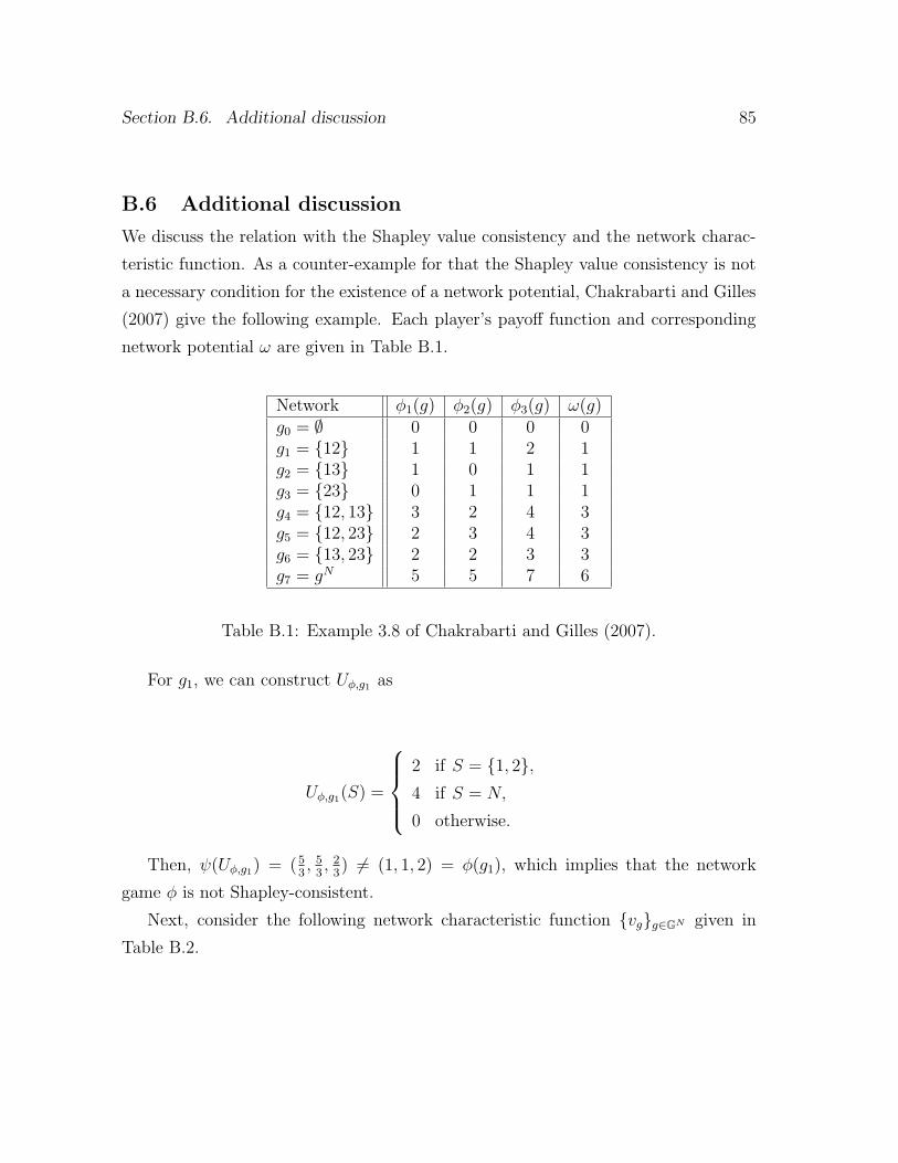
Section B.6. Additional discussion 85
B.6 Additional discussion
We discuss the relation with the Shapley value consistency and the network charac-
teristic function. As a counter-example for that the Shapley value consistency is not
a necessary condition for the existence of a network potential, Chakrabarti and Gilles
(2007) give the following example. Each player’s payoff function and corresponding
network potential ω are given in Table B.1.
Network ϕ1(g) ϕ2(g) ϕ3(g) ω(g)g0 = ∅ 0 0 0 0g1 = {12} 1 1 2 1g2 = {13} 1 0 1 1g3 = {23} 0 1 1 1g4 = {12, 13} 3 2 4 3g5 = {12, 23} 2 3 4 3g6 = {13, 23} 2 2 3 3g7 = gN 5 5 7 6
Table B.1: Example 3.8 of Chakrabarti and Gilles (2007).
For g1, we can construct Uϕ,g1 as
Uϕ,g1(S) =
2 if S = {1, 2},4 if S = N,
0 otherwise.
Then, ψ(Uϕ,g1) = (53, 53, 23) = (1, 1, 2) = ϕ(g1), which implies that the network
game ϕ is not Shapley-consistent.
Next, consider the following network characteristic function {vg}g∈GN given in
Table B.2.

86 Appendix B. Appendix to Chapter 2
vg\S {1} {2} {3} {1, 2} {1, 3} {2, 3} Nvg0 0 0 0 0 0 0 0vg1 0 0 0 −2 0 0 4vg2 0 0 0 0 2 0 2vg3 0 0 0 0 0 2 2vg4 0 0 0 −2 2 0 9vg5 0 0 0 −2 0 2 9vg6 0 0 0 0 2 2 7vg7 0 0 0 −2 2 2 17
Table B.2: An example of {vg}g∈GN such that ϕi(g) = ψi(vg).
We can show that, for any g ∈ GN , ϕ(g) = ψ(vg). Therefore, this network game
ϕ admits a network potential ω by Theorem 2.1 although it is not Shapley value
consistent.
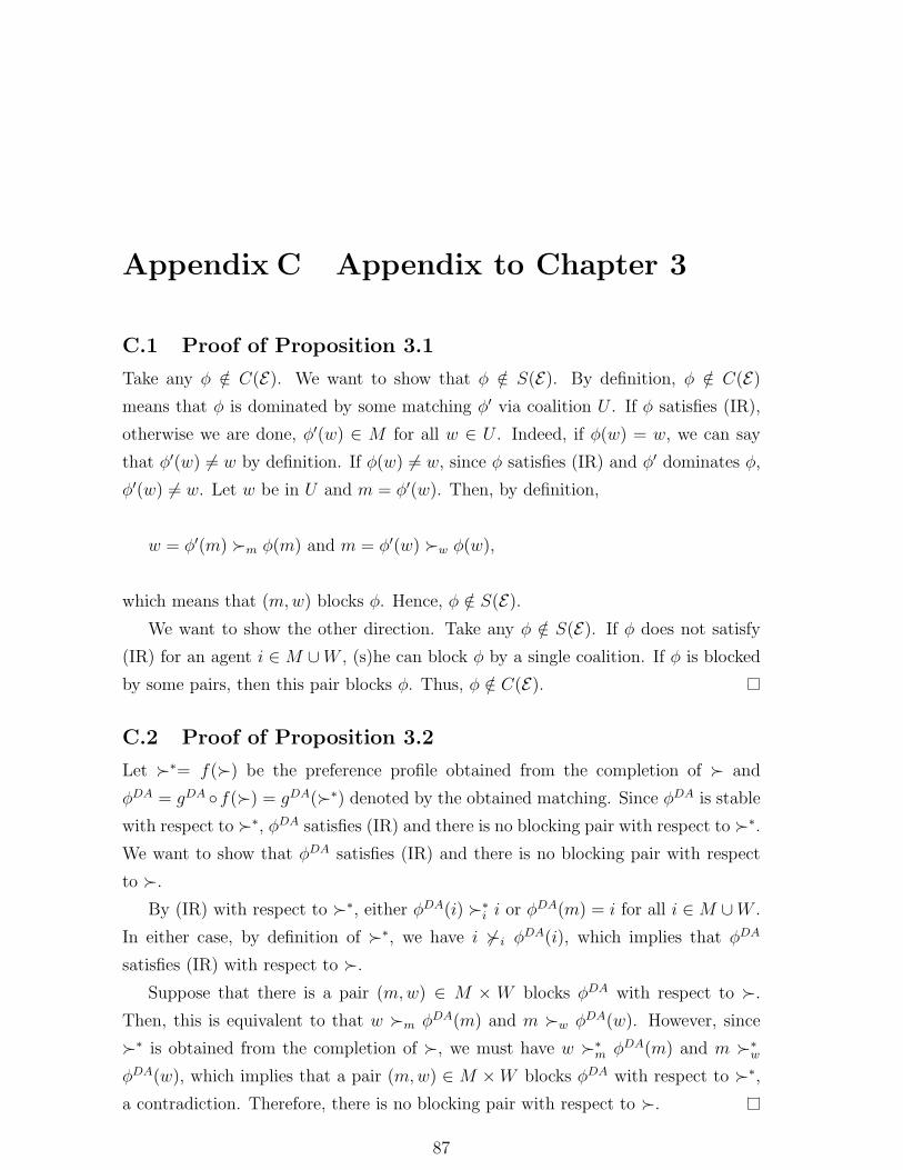
Appendix C Appendix to Chapter 3
C.1 Proof of Proposition 3.1
Take any ϕ /∈ C(E). We want to show that ϕ /∈ S(E). By definition, ϕ /∈ C(E)means that ϕ is dominated by some matching ϕ′ via coalition U . If ϕ satisfies (IR),
otherwise we are done, ϕ′(w) ∈ M for all w ∈ U . Indeed, if ϕ(w) = w, we can say
that ϕ′(w) = w by definition. If ϕ(w) = w, since ϕ satisfies (IR) and ϕ′ dominates ϕ,
ϕ′(w) = w. Let w be in U and m = ϕ′(w). Then, by definition,
w = ϕ′(m) ≻m ϕ(m) and m = ϕ′(w) ≻w ϕ(w),
which means that (m,w) blocks ϕ. Hence, ϕ /∈ S(E).We want to show the other direction. Take any ϕ /∈ S(E). If ϕ does not satisfy
(IR) for an agent i ∈M ∪W , (s)he can block ϕ by a single coalition. If ϕ is blocked
by some pairs, then this pair blocks ϕ. Thus, ϕ /∈ C(E).
C.2 Proof of Proposition 3.2
Let ≻∗= f(≻) be the preference profile obtained from the completion of ≻ and
ϕDA = gDA ◦f(≻) = gDA(≻∗) denoted by the obtained matching. Since ϕDA is stable
with respect to ≻∗, ϕDA satisfies (IR) and there is no blocking pair with respect to ≻∗.
We want to show that ϕDA satisfies (IR) and there is no blocking pair with respect
to ≻.
By (IR) with respect to ≻∗, either ϕDA(i) ≻∗i i or ϕ
DA(m) = i for all i ∈M ∪W .
In either case, by definition of ≻∗, we have i ⊁i ϕDA(i), which implies that ϕDA
satisfies (IR) with respect to ≻.
Suppose that there is a pair (m,w) ∈ M × W blocks ϕDA with respect to ≻.
Then, this is equivalent to that w ≻m ϕDA(m) and m ≻w ϕDA(w). However, since
≻∗ is obtained from the completion of ≻, we must have w ≻∗m ϕDA(m) and m ≻∗
w
ϕDA(w), which implies that a pair (m,w) ∈ M ×W blocks ϕDA with respect to ≻∗,
a contradiction. Therefore, there is no blocking pair with respect to ≻.
87

88 Appendix C. Appendix to Chapter 3
C.3 Proof of Proposition 3.3
Take any ≻∈ P as a true preference profile. Let ≻∗= f(≻) be the preference profile
obtained from the completion of ≻. Consider the hypothetical situation that ≻∗ is
a true preference profile. Since gDA is strategy-proof, for any m ∈ M , ≻′m∈ Pm and
≻−m∈ P−m, we have
gDA ◦ f(≻m,≻−m) = gDA(≻∗
m, f−m(≻))
≿∗m gDA
(fm(≻′
m,≻−m), f−m(≻′m,≻−m)
)= gDA ◦ f(≻′
m,≻−m).
Then, this implies that for any m ∈M , ≻′m∈ Pm and ≻−m∈ P−m, we have
gDA ◦ f(≻′m,≻−m) = gDA
(fm(≻′
m,≻−m), f−m(≻′m,≻−m)
)⊁m gDA
(≻∗
m, f−m(≻))
= gDA ◦ f(≻m,≻−m).
Therefore, gDA ◦ f is strategy-proof.
C.4 Proof of Proposition 3.4
Since Pr ⊂ Pacyc and f(≻) =≻ for all ≻∈ Pr, g◦f = g on Pr. Then, by the fact that
gDA is the unique mechanism which induces a stable matching and satisfies strategy-
proof for M (Dubins and Freedman, 1981; Roth, 1982, and Alcalde and Barbera,
1994), we must have g = gDA. However, we show that there exists an economy Ein which gDA ◦ f does not induce the M -optimal matching for any f ∈ F . To see
this, consider the following example. Let M = {m1,m2,m3} and W = {w1, w2, w3}.We assume that each agent is acceptable for every i ∈ M ∪W . Other specification
of preference profile is given as follows. Note that there is no other relation (i.e.,
incomparable) than the specification:
m1 : w1 ≻m1 w2 and w1 ≻m1 w3,
m2 : w1 ≻m2 w3 and w3 ≻m2 w2,
m3 : w3 ≻m3 w1 and w3 ≻m3 w2,
w1 : m3 ≻w1 m2 and m2 ≻w1 m1,

Section C.5. Relation with Bernheim and Rangel (2009) 89
w2 : m1 ≻w2 m3 and m2 ≻w2 m3,
w3 : m1 ≻w3 m2 and m3 ≻w3 m2.
In this economy, there are four stable matchings:
ϕ1 = {(m1, w1), (m2, w2), (m3, w3)}, ϕ2 = {(m1, w2), (m2, w1), (m3, w3)},
ϕ3 = {(m1, w3), (m2, w1), (m3, w2)}, ϕ4 = {(m1, w3), (m2, w2), (m3, w1)}.
Note that ϕ1 is the M -optimal matching for (≻m)m∈M . However, for any com-
pletion rule f ∈ F , ϕ1 is not stable with respect to f(≻) because w1fm2(≻)w2 and
m2fw1(≻)m1, which means that a pair (m2, w1) is a blocking pair in f(≻).1 Therefore,
gDA ◦ f does not induce ϕ1 as an outcome.
C.5 Relation with Bernheim and Rangel (2009)
We introduce a formal definition of the unambiguous preference and the core based
on the relation by Bernheim and Rangel (2009).
For each man m ∈ M , let Cm : 2W∪{m} → W ∪ {m} be a choice function for
m.2 Similarly, for each woman w ∈ W , let Cw : 2M∪{w} → M ∪ {w} be a choice
function for m. Let us call E = (M,W, (Ci)i∈M∪W ) an economy. A choice function
C is rational if there exists a strict, complete and transitive preference ≻ such that
C(X) = argmax≻X where X is an arbitrarily choice set. It is known that a choice
function is rational if and only if it satisfies so called independence of irrelevant
alternatives (hereafter, we call it IIA).3
1An example of f(≻) is as follows:m1 : w1 ≻m1
w2 ≻m1w3 ≻m1
m1,m2 : w1 ≻m2 w3 ≻m2 w2 ≻m2 m2,m3 : w3 ≻m3 w1 ≻m3 w2 ≻m3 m3,
w1 : m3 ≻w1m2 ≻w1
m1 ≻w1w1,
w2 : m2 ≻w2m1 ≻w2
m3 ≻w2w2,
w3 : m3 ≻w3m1 ≻w3
m2 ≻w3w3.
As we claimed, we can see that (m2, w1) is a blocking pair for ϕ1.2Ci(∅) = ∅ for all i ∈M ∪W for convenience.3Let X be the whole set of choice alternatives. We say that a choice function C : 2X → X satisfies
IIA if for any X,Y such that Y ⊂ X, if C(X) ∈ C(Y ), then C(X) = C(Y ). Also, this condition is
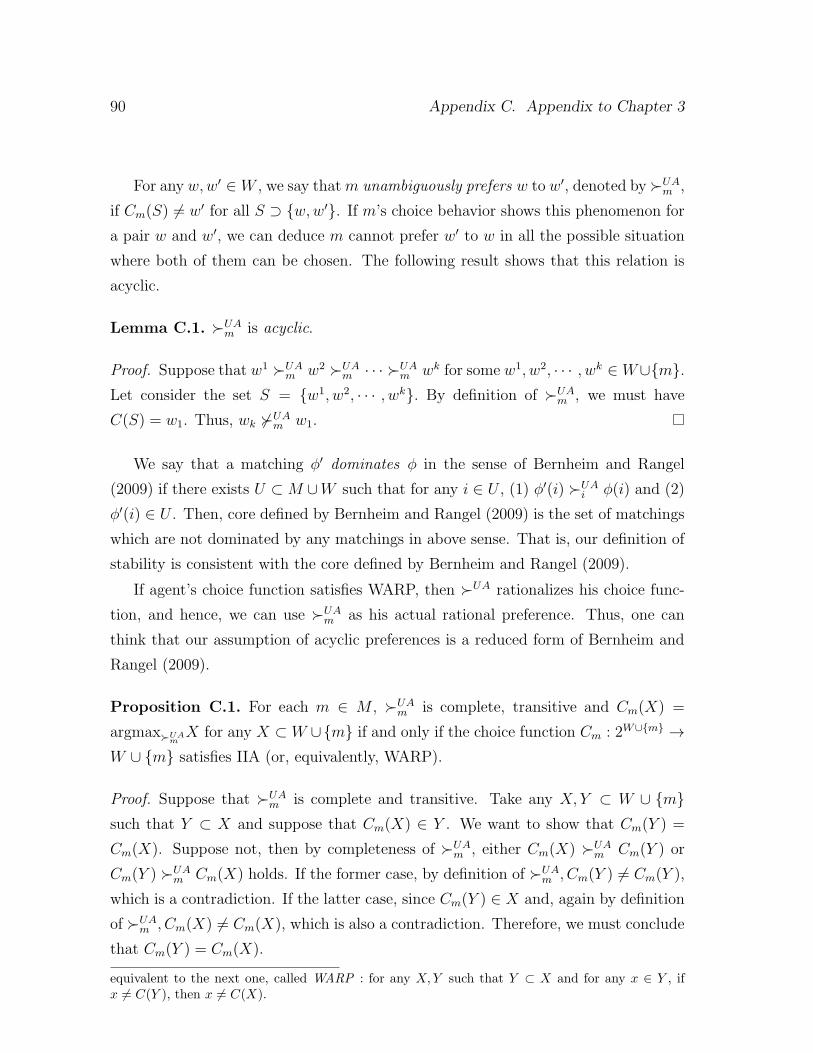
90 Appendix C. Appendix to Chapter 3
For any w,w′ ∈ W , we say thatm unambiguously prefers w to w′, denoted by≻UAm ,
if Cm(S) = w′ for all S ⊃ {w,w′}. If m’s choice behavior shows this phenomenon for
a pair w and w′, we can deduce m cannot prefer w′ to w in all the possible situation
where both of them can be chosen. The following result shows that this relation is
acyclic.
Lemma C.1. ≻UAm is acyclic.
Proof. Suppose that w1 ≻UAm w2 ≻UA
m · · · ≻UAm wk for some w1, w2, · · · , wk ∈ W∪{m}.
Let consider the set S = {w1, w2, · · · , wk}. By definition of ≻UAm , we must have
C(S) = w1. Thus, wk ⊁UAm w1.
We say that a matching ϕ′ dominates ϕ in the sense of Bernheim and Rangel
(2009) if there exists U ⊂M ∪W such that for any i ∈ U , (1) ϕ′(i) ≻UAi ϕ(i) and (2)
ϕ′(i) ∈ U . Then, core defined by Bernheim and Rangel (2009) is the set of matchings
which are not dominated by any matchings in above sense. That is, our definition of
stability is consistent with the core defined by Bernheim and Rangel (2009).
If agent’s choice function satisfies WARP, then ≻UA rationalizes his choice func-
tion, and hence, we can use ≻UAm as his actual rational preference. Thus, one can
think that our assumption of acyclic preferences is a reduced form of Bernheim and
Rangel (2009).
Proposition C.1. For each m ∈ M , ≻UAm is complete, transitive and Cm(X) =
argmax≻UAmX for any X ⊂ W ∪{m} if and only if the choice function Cm : 2W∪{m} →
W ∪ {m} satisfies IIA (or, equivalently, WARP).
Proof. Suppose that ≻UAm is complete and transitive. Take any X,Y ⊂ W ∪ {m}
such that Y ⊂ X and suppose that Cm(X) ∈ Y . We want to show that Cm(Y ) =
Cm(X). Suppose not, then by completeness of ≻UAm , either Cm(X) ≻UA
m Cm(Y ) or
Cm(Y ) ≻UAm Cm(X) holds. If the former case, by definition of ≻UA
m , Cm(Y ) = Cm(Y ),
which is a contradiction. If the latter case, since Cm(Y ) ∈ X and, again by definition
of ≻UAm , Cm(X) = Cm(X), which is also a contradiction. Therefore, we must conclude
that Cm(Y ) = Cm(X).
equivalent to the next one, called WARP : for any X,Y such that Y ⊂ X and for any x ∈ Y , ifx = C(Y ), then x = C(X).

Section C.5. Relation with Bernheim and Rangel (2009) 91
Next, we show the other direction. Suppose that the choice function Cm : 2W∪{m} →W ∪ {m} satisfies IIA (and hence, it satisfies WARP). Take any w,w′ ∈ W ∪ {m}and suppose that, without loss of generality, Cm({w,w′}) = w. Then by WARP, for
any X ⊂ W ∪ {m} such that {w,w′} ⊂ X,w′ = Cm(X). This means that w ≻UAm w′.
Since this is satisfied for any pair w,w′ ∈ W ∪ {m}, ≻UAm is complete, i.e., for any
w,w′ ∈ W ∪ {m}, Cm({w,w′}) = w ⇔ w ≻UAm w′. Then, suppose that w ≻UA
m w′
and w′ ≻UAm w′′. Then, Cm({w,w′, w′′}) = w. By WARP, for any X ⊂ W ∪ {m}
such that {w,w′′} ⊂ X,w′′ = Cm(X). Thus, w ≻UAm w′′, which implies that ≻UA
m is
transitive. Finally, by definition of ≻UA, x = Cm(X) implies that y ⊁UAm x for all
y ∈ X\{x} and X ⊂ W ∪ {m}. Since ≻UAm is complete, x ⊁UA
m y, which implies
Cm(X) = argmax≻UAmX for any X ⊂ W ∪ {m}.

Appendix D Appendix to Chapter 4
D.1 Proof of Theorem 4.2
Let Gc ⊂ G denote the set of games such that v(N) = c. Also, for any player i ∈ N and
c ∈ R, let Gc,i denote the set of games such that v(N) = c and i is null player. Note
that Gc,i ⊂ Gc for all i ∈ N and c ∈ R. Let ∆i(v) = (v(S∪{i})−v(S))S⊆N\{i} ∈ R2(N−1)
be a vector of marginal contributions of i in v. Therefore player i ∈ N is a null player
in v if ∆i(v) = 0. Let Λi be the set of all vectors of marginal contribution of i:
Λi = {∆i(v)|v ∈ G}.For each x ∈ RN , letmx ∈ G be an additive game, mx(S) =
∑i∈S xi for all S ⊆ N .
Let Gadd be the set of additive games. Since there is a one-to-one correspondence
between x ∈ RN and an additive game mx, we can identify Gadd with RN . Abe and
Nakada (2017) provide the following result, which can be useful later.
Theorem D.1 (Abe and Nakada, 2017). Let n = 2. f : Gadd → Rn satisfies (E),
(M−), (NY), and (RIN) if and only if there exists a δ ∈ [0, 1] and a w ∈ W such that
fi(x) = δ · xi + (1− δ) · wi ·∑
l∈N xl for all x ∈ Rn and i ∈ N .
Now, we offer the proof of Theorem 4.2. It is clear that the rule satisfies all the
axioms. We suppose that a rule f : G → RN satisfies (E), (M−), (RIN), (WDMSP),
and (NY).
Claim 1: For each i ∈ N , there exist functions ϕi : Λi×R → R and αi : R → R such
that fi(v) = ϕi(∆i(v), v(N)) + αi(v(N)).
We first take any c ∈ R. For any i ∈ N and v ∈ Gc, we have the following
equation: for any v ∈ Gc such that ∆i(v) = ∆i(v),
fi(v)(M−)= fi(v) =: αi(c,∆i(v)). (D.1)
Specifically, we denote
αi(c) = αi(c,0). (D.2)
92
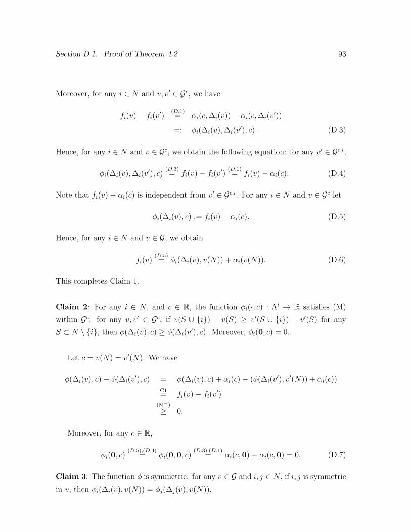
Section D.1. Proof of Theorem 4.2 93
Moreover, for any i ∈ N and v, v′ ∈ Gc, we have
fi(v)− fi(v′)
(D.1)= αi(c,∆i(v))− αi(c,∆i(v
′))
=: ϕi(∆i(v),∆i(v′), c). (D.3)
Hence, for any i ∈ N and v ∈ Gc, we obtain the following equation: for any v′ ∈ Gc,i,
ϕi(∆i(v),∆i(v′), c)
(D.3)= fi(v)− fi(v
′)(D.1)= fi(v)− αi(c). (D.4)
Note that fi(v)− αi(c) is independent from v′ ∈ Gc,i. For any i ∈ N and v ∈ Gc let
ϕi(∆i(v), c) := fi(v)− αi(c). (D.5)
Hence, for any i ∈ N and v ∈ G, we obtain
fi(v)(D.5)= ϕi(∆i(v), v(N)) + αi(v(N)). (D.6)
This completes Claim 1.
Claim 2: For any i ∈ N , and c ∈ R, the function ϕi(·, c) : Λi → R satisfies (M)
within Gc: for any v, v′ ∈ Gc, if v(S ∪ {i}) − v(S) ≥ v′(S ∪ {i}) − v′(S) for any
S ⊂ N \ {i}, then ϕ(∆i(v), c) ≥ ϕ(∆i(v′), c). Moreover, ϕi(0, c) = 0.
Let c = v(N) = v′(N). We have
ϕ(∆i(v), c)− ϕ(∆i(v′), c) = ϕ(∆i(v), c) + αi(c)− (ϕ(∆i(v
′), v′(N)) + αi(c))
C1= fi(v)− fi(v
′)(M−)
≥ 0.
Moreover, for any c ∈ R,
ϕi(0, c)(D.5),(D.4)
= ϕi(0,0, c)(D.3),(D.1)
= αi(c,0)− αi(c,0) = 0. (D.7)
Claim 3: The function ϕ is symmetric: for any v ∈ G and i, j ∈ N , if i, j is symmetric
in v, then ϕi(∆i(v), v(N)) = ϕj(∆j(v), v(N)).
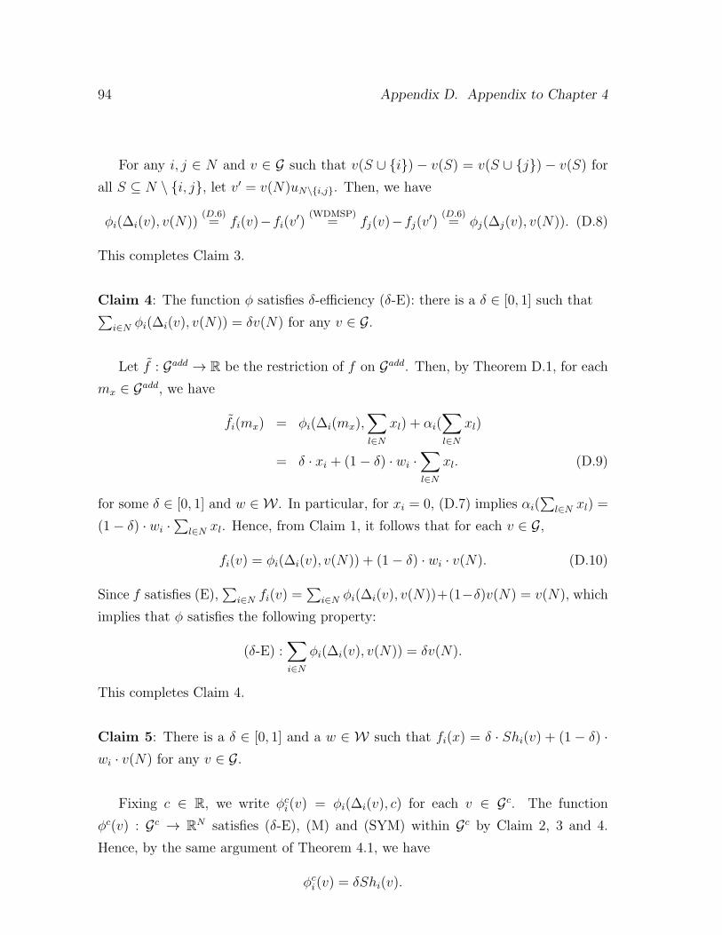
94 Appendix D. Appendix to Chapter 4
For any i, j ∈ N and v ∈ G such that v(S ∪ {i}) − v(S) = v(S ∪ {j}) − v(S) for
all S ⊆ N \ {i, j}, let v′ = v(N)uN\{i,j}. Then, we have
ϕi(∆i(v), v(N))(D.6)= fi(v)−fi(v′)
(WDMSP)= fj(v)−fj(v′)
(D.6)= ϕj(∆j(v), v(N)). (D.8)
This completes Claim 3.
Claim 4: The function ϕ satisfies δ-efficiency (δ-E): there is a δ ∈ [0, 1] such that∑i∈N ϕi(∆i(v), v(N)) = δv(N) for any v ∈ G.
Let f : Gadd → R be the restriction of f on Gadd. Then, by Theorem D.1, for each
mx ∈ Gadd, we have
fi(mx) = ϕi(∆i(mx),∑l∈N
xl) + αi(∑l∈N
xl)
= δ · xi + (1− δ) · wi ·∑l∈N
xl. (D.9)
for some δ ∈ [0, 1] and w ∈ W . In particular, for xi = 0, (D.7) implies αi(∑
l∈N xl) =
(1− δ) · wi ·∑
l∈N xl. Hence, from Claim 1, it follows that for each v ∈ G,
fi(v) = ϕi(∆i(v), v(N)) + (1− δ) · wi · v(N). (D.10)
Since f satisfies (E),∑
i∈N fi(v) =∑
i∈N ϕi(∆i(v), v(N))+(1−δ)v(N) = v(N), which
implies that ϕ satisfies the following property:
(δ-E) :∑i∈N
ϕi(∆i(v), v(N)) = δv(N).
This completes Claim 4.
Claim 5: There is a δ ∈ [0, 1] and a w ∈ W such that fi(x) = δ · Shi(v) + (1 − δ) ·wi · v(N) for any v ∈ G.
Fixing c ∈ R, we write ϕci(v) = ϕi(∆i(v), c) for each v ∈ Gc. The function
ϕc(v) : Gc → RN satisfies (δ-E), (M) and (SYM) within Gc by Claim 2, 3 and 4.
Hence, by the same argument of Theorem 4.1, we have
ϕci(v) = δShi(v).

Section D.2. Independence of axioms for Theorem 4.2 95
Since c ∈ R is arbitrarily chosen, for any v ∈ G, we have
ϕi(∆i(v), v(N)) = ϕv(N)i (v) = δShi(v) (D.11)
Finally, by (D.10) and (D.11), we obtain fi(x) = δ ·Shi(v)+ (1− δ) ·wi · v(N), which
completes the proof.
D.2 Independence of axioms for Theorem 4.2
The independence of the axioms is shown in the examples listed below.
Example D.2.1. Consider the following function: for any i ∈ N and v ∈ G,
fEi (v) = 0.
This function satisfies all axioms except (E).
Example D.2.2. Consider the following function: for any i ∈ N and v ∈ G,
fM−
i (v) = 2Shi(v)−v(N)
n.
This function satisfies all axioms except (M−).
Example D.2.3. Consider the following function: for any i ∈ N and v ∈ G,
fRINi (v) = δShi + (1− δ)
i+ v(N)2
N + n(v(N))2v(N),
where N =∑
i∈N i =n(n−1)
2and i is the natural number representing player i. This
rule satisfies (E), (M−), (WMDSP) and (NY) but not (RIN). To check (M−), let
hi(a) = i+a2
N+a2a = ia+a3
N+a2. Then, we have dhi(a)
da= na4+(3N−ni)a2+iN
(N+a2)2> 0 for all a ∈ R
because na4 + iN > 0 for all i and 3N − ni ≥ n(n−3)2
≥ 0.
Example D.2.4. Fix a permutation of all players σ. Consider the following function:
for any i ∈ N and v ∈ G,
fWMDSPi (v) = v(P σ
i ∪ {i})− v(P σi )

96 Appendix D. Appendix to Chapter 4
where P σi is the set of predecessors of i in σ. This function satisfies all the axioms
except (WMDSP).
Example D.2.5. Consider the following function: for any i ∈ N and v ∈ G,
fNYi (v) =
{Sh1 + 10 if i = 1,
Shi − 10n−1
if i = 1.
This rule satisfies all the axioms except (NY).
D.3 A counterexample to Theorem 4.2 and 4.3 for n = 2
Theorem 4.2 and 4.3 fail for n = 2. Consider the following allocation rule f♡ on
N = {1, 2}:
(f♡1 (v, w), f
♡2 (v, w)) =
(Sh1(v), Sh2(v)), Sh1(v) ≥ 0 and Sh2(v) ≥ 0,
(0, v(N)), Sh1(v) < 0 and Sh2(v) > 0 ∧ v(N) ≥ 0,
(v(N), 0), Sh1(v) < 0 and Sh2(v) > 0 ∧ v(N) < 0,
(Sh1(v), Sh2(v)), Sh1(v) ≤ 0 and Sh2(v) ≤ 0,
(0, v(N)), Sh1(v) > 0 and Sh2(v) < 0 ∧ v(N) ≤ 0,
(v(N), 0), Sh1(v) > 0 and Sh2(v) < 0 ∧ v(N) > 0,
for any v ∈ G and w ∈ W .
Note that this function does not depend on w. It is clear that f♡ satisfies (E∗) and
(M−∗). It satisfies (SYM∗) because if the players 1 and 2 are symmetric in the sense
of marginal contribution and have the same weight, they receive (Sh1(v), Sh2(v)). It
satisfies (RIN∗) because if the players 1 and 2 are null players, the game v is the null
game: v(12) = v(1) = v(2) = 0. Since f♡ does not depend on w, it clearly satisfies
(FEC∗). By the same argument, the uniqueness for Theorem 4.2 fails for n = 2.
D.4 Proof of Theorem 4.3
We first show that (E∗), (M−∗), (SYM∗) characterizes the egalitarian Shapley value
when we fix w = ( 1n, ..., 1
n), which can be useful in later.
Lemma D.1. Suppose that W = {( 1n, ..., 1
n)} and n = 2. Then, an allocation rule
f : G × W → RN satisfies (E∗), (M−∗), (SYM∗) if and only if it is an egalitarian-
Shapley value.

Section D.4. Proof of Theorem 4.3 97
Proof. This follows from the axioms and arguments in Casajus and Huettner (2014)
if w = ( 1n, ..., 1
n).
Now, we offer the proof of Theorem 4.3. It is clear that the rule satisfies all the
axioms. We suppose that a rule f : G → RN satisfies (E∗), (M−∗), (RIN∗), (SYM∗),
and (FEC∗). Claim 1 can be thought of as an analog of that of Theorem 4.2. The
differences lie in Claims 2-4. In this proof, we first specify the form of the Shapley
value, while we first specify the weighted division in Theorem 4.2.
Claim 1: For each i ∈ N , there exists functions ϕi(v) : Λi×R → R and αi : W×R →
R such that fi(v, w) = ϕi(∆i(v), v(N)) + αi(w, v(N)).
We first take any c ∈ R. For any i ∈ N , v ∈ G and w ∈ W , we have the following
equation: for any v ∈ Gc such that ∆i(v) = ∆i(v),
fi(v, w)(M−∗)= fi(v, w) =: αi(w, c,∆i(v)). (D.12)
Specifically, we denote
αi(w, c) = αi(w, c,0). (D.13)
By (FEC∗), for any c ∈ R and i ∈ N , there is a function ϕci : Gc → R such that
ϕci(v) = fi(v, w)− fi(cuN\{i}, w)
(D.13)= fi(v, w)− αi(w, c).
By (D.12), we know that ϕci(v) = ϕc
i(v) if v(N) = v(N) = c and ∆i(v) = ∆i(v).
Hence, we can define ϕi(∆i(v), c) : Λi × R → R as ϕi(∆i(v), c) =: ϕc
i(v). Therefore,
for any i ∈ N , v ∈ G and w ∈ W , we obtain fi(v, w) = ϕi(∆i(v), v(N))+αi(w, v(N)).
This completes Claim 1.
Claim 2: For any v ∈ G, there exists a δ ∈ [0, 1] and dv(N)i ∈ R such that
ϕi(∆i(v), v(N)) = δShi(v) + dv(N)i .
Let w∗ = (1/n, · · · , 1/n) ∈ W , i.e., the equal weight. For any c ∈ R and any
v ∈ Gc, by Claim 1, we have
fi(v, w∗) = ϕi(∆i(v), v(N)) + αi(w
∗, v(N)), (D.14)

98 Appendix D. Appendix to Chapter 4
and, by Lemma D.1, there exists δ ∈ [0, 1] such that
fi(v, w∗) = δShi(v) + (1− δ)
1
nc. (D.15)
Note that δ does not depend on c ∈ R. For any v′ ∈ Gc,i, we have
ϕi(∆i(v′), c) + αi(w
∗, c)(D.14)= fi(v
′, w∗)(D.15)= δShi(v
′) + (1− δ)1
nc
= (1− δ)1
nc. (D.16)
Note that player i is a null player in game v′ ∈ Gc,i. Hence, for any v′, v′′ ∈ Gc,i, we
have ϕi(∆i(v′), c) + αi(w
∗, c)(D.16)= (1 − δ) 1
nc
(D.16)= ϕi(∆i(v
′′), c) + αi(w∗, c) and, so,
denote dci := ϕi(∆i(v′), c) = ϕi(∆i(v
′′), c). We obtain
αi(w∗, c)
(D.16),dci= (1− δ)1
nc− dci . (D.17)
Therefore, for every v ∈ Gc, we must have
ϕi(∆i(v), c)(D.14)(D.15)(D.17)
= δShi(v) + dci . (D.18)
Since c ∈ R is arbitrary chosen, we obtain ϕi(∆i(v′), v(N)) = δShi(v) + d
v(N)i for all
v ∈ G.
Claim 3: αi(w, v(N)) = (1− δ) · wiv(N)− dv(N)i for each w ∈ W .
Consider any w ∈ W and player k∗ ∈ N such that k∗ ∈ argmini∈N,wi>0wi. Note
that k∗ is well-defined because∑
i∈N wi = 1 and wi ≥ 0 for any i ∈ N . By Claim 2,
for any player i = k∗ and any c ∈ R,
fk(cu{i}, w) =
{δc+ dck + αk(w, c) if k = i,
dck + ψck(w) otherwise.
Hence, we have ∑k∈N
(αk(w, c) + dck)(E∗)= (1− δ)c. (D.19)
Moreover, for any i = k∗, j (j = i, j = k∗) and, by considering a game cu{j}, we have
αi(w, c) + dci(RIN∗)=
wi
wk∗(αk∗(w, c) + dck∗), (D.20)
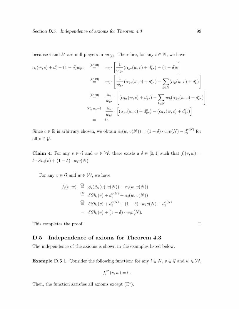
Section D.5. Independence of axioms for Theorem 4.3 99
because i and k∗ are null players in cu{j}. Therefore, for any i ∈ N , we have
αi(w, c) + dci − (1− δ)wic(D.20)= wi ·
[1
wk∗(αk∗(w, c) + dck∗)− (1− δ)c
](D.19)= wi ·
[1
wk∗(αk∗(w, c) + dck∗)−
∑k∈N
(αk(w, c) + dck)
](D.20)=
wi
wk∗·
[(αk∗(w, c) + dck∗)−
∑k∈N
wk(αk∗(w, c) + dck∗)
]∑
k wk=1=
wi
wk∗·[(αk∗(w, c) + dck∗)− (αk∗(w, c) + dck∗)
]= 0.
Since c ∈ R is arbitrary chosen, we obtain αi(w, v(N)) = (1− δ) · wiv(N)− dv(N)i for
all v ∈ G.
Claim 4: For any v ∈ G and w ∈ W , there exists a δ ∈ [0, 1] such that fi(v, w) =
δ · Shi(v) + (1− δ) · wiv(N).
For any v ∈ G and w ∈ W , we have
fi(v, w)C1= ϕi(∆i(v), v(N)) + αi(w, v(N))
C2= δShi(v) + d
v(N)i + αi(w, v(N))
C3= δShi(v) + d
v(N)i + (1− δ) · wiv(N)− d
v(N)i
= δShi(v) + (1− δ) · wiv(N).
This completes the proof.
D.5 Independence of axioms for Theorem 4.3
The independence of the axioms is shown in the examples listed below.
Example D.5.1. Consider the following function: for any i ∈ N , v ∈ G and w ∈ W ,
fE∗
i (v, w) = 0.
Then, the function satisfies all axioms except (E∗).

100 Appendix D. Appendix to Chapter 4
Example D.5.2. Consider the following function: for any i ∈ N , v ∈ G and w ∈ W ,
fM−∗
i (v, w) = 2Shi(v)− wiv(N).
Then, the function satisfies all axioms except (M−∗).
Example D.5.3. Consider the following function: for any i ∈ N , v ∈ G and w ∈ W ,
fRIN∗
i (v, w) = δ · v(N)
|N |+ (1− δ) · wiv(N).
The function satisfies all axioms except (RIN∗).
Example D.5.4. Consider the following function: for any i ∈ N , v ∈ G and w ∈ W ,
fSYM∗
i (v, w) = δ · Shzi (v) + (1− δ) · wiv(N),
where Shzi (v) is the weighted Shapley value for a given weight z ∈ RN++. Since (SYM
∗)
is defined over G and W , the function satisfies all axioms except (SYM∗).
Example D.5.5. Consider the following function: for any i ∈ N , v ∈ G and w ∈ W ,
fFEC∗
i (v, w) = wmin · Shi(v) + (1− wmin)wiv(N),
where wmin = minj∈N wj. This function satisfies all axioms except (FEC∗).
Appendix E Appendix to Chapter 5
E.1 Other robustness concepts
In this appendix, we consider two other robustness concepts.
Strong robustness and a SMR
Even if a voting rule is robust and responsiveness of at least one individual is strictly
greater than one-half, the arithmetic mean of responsiveness of all individuals can be
less than one-half, which implies that a collective decision reflects minority preferences
on average. To avoid this scenario, a voting rule must satisfy the following stronger
requirement.
Definition E.1. A voting rule ϕ ∈ Φ is strongly robust if, for each p ∈ ∆(X ), the
arithmetic mean of responsiveness is strictly greater than one-half:∑i∈N
p(ϕ(x) = xi)/n > 1/2 for all p ∈ ∆(X ). (E.1)
Clearly, a strongly robust rule is robust. In the next proposition, we show that a
voting rule is strongly robust if and only if it is robust and anonymous; that is, it is
a SMR with odd n.
Proposition E.1. Suppose that n is odd. Then, a voting rule is strongly robust if
and only if it is a SMR. Suppose that n is even. Then, no voting rule is strongly
robust.
Proof. Note that, by (5.1), (E.1) is equivalent to∑i∈N
Ep[ϕ(x)xi] > 0 for all p ∈ ∆(X ). (E.2)
Suppose that n is odd and that ϕ is a SMR. Then, ϕ satisfies (E.2) by Lemma
5.1, so a SMR is strongly robust.
Suppose that ϕ is not a SMR. Then, there exist y ∈ X and S ⊊ N such that
|S| < n/2 and ϕ(y) = yi if and only if i ∈ S. Let p ∈ ∆(X ) be such that p(y) = 1.
101

102 Appendix E. Appendix to Chapter 5
Then,∑
i∈N Ep[ϕ(x)xi] = |S| − |N \ S| < 0, violating (E.2). Thus, a voting rule is
not strongly robust unless it is a SMR.
Suppose that n is even. Let y ∈ X be such that yi = 1 for i ≤ n/2 and yi = −1
for i ≥ n/2 + 1. For p ∈ ∆(X ) with p(y) = 1 and any ϕ ∈ Φ, it holds that∑i∈N Ep[ϕ(x)xi] = 0, violating (E.2). Thus, no voting rule is strongly robust when n
is even.
Semi-robustness and a WMR
We consider the following weaker version of robustness to characterize a WMR with
possibly negative weights.
Definition E.2. A voting rule ϕ ∈ Φ is semi-robust if, for each p ∈ ∆(X ), respon-
siveness of at least one individual is not equal to one-half.
To understand the implication of semi-robustness, imagine that some individuals
are more likely to have correct choices and other individuals are more likely to have
wrong choices. However, if the responsiveness of every individual is equal to one-
half, then it is difficult to extract information from individuals in order to arrive
at a correct group decision. A semi-robust rule does not face this problem for any
probability distribution.
The following proposition establishes the equivalence of a semi-robust rule and a
WMR with possibly negative weights allowing no ties.
Proposition E.2. A voting rule is semi-robust if and only if it is a WMR such that
there are no ties.
To prove Proposition E.2, we use the following theorem of alternatives, which is
referred to as Gordan’s theorem. This result also appears in Gale (1960, Theorems
2.9) as a corollary of Farkas’ lemma.
Lemma E.1. Let A be an n ×m matrix. Exactly one of the following alternatives
holds.
• There exists ξ ∈ Rn satisfying
ξ⊤A≫ 0.
• There exists η ∈ Rm satisfying
Aη = 0, η > 0.

Section E.2. An imaginary asset market 103
Proof of Proposition E.2. We can restate the conditions in Proposition E.2 as follows.
(a′′) By Lemma 5.1, a voting rule ϕ is a WMR allowing no ties if and only if there
exists w = (wi)i∈N = 0 such that∑i∈N
wilij =∑i∈N
wi
(ϕ(xj)xji
)> 0
for each j ∈M , or equivalently, w⊤L≫ 0.
(b′′) By definition, a voting rule is not semi-robust if and only if there exists p =
(pj)j∈M > 0 such that∑j∈N
lijpj =∑
j:ϕ(xj)=xji
pj −∑
j:ϕ(xj)=xji
pj = 0
for each i ∈ N , or equivalently, Lp = 0.
Proposition E.2 states that exactly one of (a′′) and (b′′) holds, which is true by
Lemma E.1. In fact, by plugging L, w, and p into A, ξ, and η in Lemma E.1,
respectively, we can conclude that exactly one of (a′′) and (b′′) holds.
E.2 An imaginary asset market
We can explain why Proposition 5.1 is true in terms of arbitrage-free pricing in an
imaginary asset market because we can interpret Lemma 5.4 as a corollary of the
fundamental theorem of asset pricing.
Let M and N be the set of states and the set of assets, respectively. One unit of
asset i ∈ N yields a payoff lij when state j ∈ M is realized. Recall that lij equals
+1 if i’s choice agrees with the collective decision and −1 otherwise. The matrix L
is referred to as the payoff matrix. We denote by q = (qi)i∈N the vector of prices of
the n assets.
A portfolio defined by a vector w = (wi)i∈N consists of wi units of asset i for each
i ∈ N . It yields a payoff∑
i∈N wilij when state j ∈M is realized, which is summarized
in w⊤L = (∑
i∈N wilij)j∈M . The price of the portfolio is w⊤q =∑
i∈N qiwi.
We say that a price vector q is arbitrage-free if w⊤L ≥ 0 implies w⊤q ≥ 0; that is,
the price of any portfolio yielding a nonnegative payoff in each state is nonnegative.
We say that a price vector q is determined by a nonnegative linear pricing rule if there

104 Appendix E. Appendix to Chapter 5
exists a nonnegative vector p = (pj)j∈M > 0, which is referred to as a state price, such
that q = Lp. The fundamental theorem of asset pricing establishes the equivalence of
an arbitrage-free price and the existence of a nonnegative linear pricing rule, which
is immediate from Farkas’ lemma.
Claim E.1. A price vector q is arbitrage-free if and only if it is determined by a
nonnegative linear pricing rule. That is, the set of all arbitrage-free price vectors is
{q : q = Lp, p > 0}.
The fundamental theorem of asset pricing has the following corollary, which is
immediate from Lemma 5.4 (a corollary of Farkas’ lemma).
Claim E.2. There exists a portfolio with nonnegative weights in all assets (i.e. no
short selling) yielding a strictly positive payoff in each state if and only if, for any
arbitrage-free price vector, the price of at least one asset is strictly positive.
The former condition is restated as w⊤L ≫ 0 for some w ≥ 0 and the latter
condition is restated as Lp ≤ 0 for all p > 0. Therefore, Claim E.2 implies the
equivalence of a robust rule and a WMR with nonnegative weights allowing no ties.
This paper does not discuss how to find optimal weights of WMRs, whereas it is a
central topic in modern portfolio theory to determine optimal weights. Thus, modern
portfolio theory could be useful to find optimal weights of WMRs.
E.3 Robustness vs. optimality
In this appendix, we demonstrate that the RTF theorem has another normative im-
plication, optimality in terms of Paretian social preferences.
Definition E.3. Fix p ∈ ∆(X ). A voting rule ϕ ∈ Φ is optimal with respect to a
Paretian von Neumann-Morgenstern (vNM) welfare function if there exists a linear
welfare function v : co(Φ) → R such that (i) Ep[ϕ′(x)xi] ≥ Ep[ϕ
′′(x)xi] for each i ∈ N
implies v(ϕ′) ≥ v(ϕ′′) for ϕ′, ϕ′′ ∈ co(Φ), and (ii) v(ϕ) ≥ v(ϕ′) for all ϕ′ ∈ co(Φ).
Harsanyi’s utilitarianism theorem (Harsanyi, 1955) states that if a linear welfare
function v : co(Φ) → R satisfies the condition (i), then there exists a nonnegative
vector w > 0 such that v(ϕ) =∑
i∈N wiE[ϕ(x)xi] for each ϕ ∈ co(Φ) (cf. Domo-
tor,1979; Weymark, 1993; Mandler, 2005). Thus, Proposition 5.3 can be understood
as the following normative characterization of WMRs.

Section E.4. Robustness vs. efficiency: a numerical example 105
Corollary E.1. Fix p ∈ ∆(X )◦. A voting rule is optimal with respect to a Paretian
vNM welfare function if and only if it is a WMR with nonnegative weights.
This corollary and Propositions 5.1 and 5.2 reveal the following relationship be-
tween robustness, weak robustness, and optimality.
Corollary E.2. A voting rule is optimal with respect to a Paretian vNM welfare
function if and only if it is weakly robust. A robust rule is optimal, but an optimal
rule is not necessarily robust.
E.4 Robustness vs. efficiency: a numerical example
In this appendix, we demonstrate the difference between the requirement of robustness
and that of efficiency using a numerical example.
Assume that n = 5 and let ϕ be a SMR with veto power of individual 1, which
can be represented as follows:
ϕ(x) =
−x1 if x ∈ A,
x1 otherwise,
where A ≡ {x ∈ X : x1 = 1, #{i : xi = 1} ≤ 2}. Fix p ∈ ∆(X ) with
p(x) =
α if x ∈ A,
β otherwise,
where 0 < α < 1/140 and β = (1 − 5α)/27. Then, no deterministic voting rule is
better than ϕ under p. To see this, let ϕ′ ∈ Φ be as good as ϕ under p. It is enough
to show that ϕ′ = ϕ. We first prove that ϕ′(x) = ϕ(x) for all x ∈ A. This is because
otherwise there exists x ∈ A such that ϕ′(x)x1 = −1 and thus the expected payoff of
individual 1 under ϕ′ is strictly less that that under ϕ:
Ep[ϕ(x)x1]− Ep[ϕ′(x)x1] =
∑x∈A
p(x)(ϕ(x)x1 − ϕ′(x)x1) +∑x∈A
p(x)(ϕ(x)x1 − ϕ′(x)x1)
=∑x∈A
β(1− ϕ′(x)x1) +∑x∈A
α(−1− ϕ′(x)x1)
≥ 2β − 10α = 2(1− 140α)/27 > 0.
106 Appendix E. Appendix to Chapter 5
We next prove that ϕ′(x) = ϕ(x) for all x ∈ A. By the above property of ϕ′, we
obtain
∑i∈N
Ep[ϕ(x)xi]−∑i∈N
Ep[ϕ′(x)xi] = α
∑x∈A
(∑i∈N
ϕ(x)xi −∑i∈N
ϕ′(x)xi
)≥ 0,
where the last inequality follows from∑
i∈N ϕ(x)xi = |∑
i∈N xi| ≥∑
i∈N ϕ′(x)xi
for all x ∈ A. We also have∑
i∈N Ep[ϕ(x)xi] ≤∑
i∈N Ep[ϕ′(x)xi] because ϕ
′ is as
good as ϕ under p. Thus,∑
i∈N Ep[ϕ(x)xi] =∑
i∈N Ep[ϕ′(x)xi], which implies that∑
i∈N ϕ(x)xi =∑
i∈N ϕ′(x)xi for all x ∈ A, i.e., ϕ′(x) = ϕ(x) for all x ∈ A.
Let us discuss whether ϕ is efficient. Although no deterministic voting rule is
better than ϕ under p, the following random voting rule ϕ′ is strictly better than ϕ
under p:
ϕ′(x) =
−1 + δ if x1 = −1 and xi = 1 for all i = 1,
−1 + γ if x1 = 1 and #{i : xi = 1} = 2,
ϕ(x) otherwise,
where δ, γ ∈ (0, 1) and βδ/(4α) < γ < βδ/(2α). In fact,
Ep[ϕ′(x)x1]− Ep[ϕ(x)x1] = −βδ + 4αγ > 0,
Ep[ϕ′(x)xi]− Ep[ϕ(x)xi] = βδ − 2αγ > 0 for each i = 1.
Thus, ϕ does not satisfy the requirement of weakly efficiency as well as that of effi-
ciency.
Let us discuss whether ϕ is robust. Although the inverse rule of ϕ is not better
than ϕ under p, it is strictly better than ϕ under p′ ∈ ∆(X ) given by
p′(x) =
1/16 if x1 = 1 and xi = −1 for all i = 1,
2/16 if x1 = 1 and #{i : xi = 1} = 2,
7/16 if x1 = −1 and xi = 1 for all i = 1,
0 otherwise.
In fact, Ep′ [ϕ(x)xi] = 7/16 − 9/16 = −1/8 < 0 for all i. Thus, if ϕ′ is the inverse
rule of ϕ then Ep′ [ϕ′(x)xi] = −Ep′ [ϕ(x)xi] > Ep′ [ϕ(x)xi] for all i, which implies that
ϕ does not satisfy the requirement of weak robustness as well as that of robustness.
Section E.5. Proof of Proposition 5.4 107
E.5 Proof of Proposition 5.4
We first prove the first statement, which asserts that exactly one of the following
holds.
(a′′′) Note that, by Lemma 5.1, a voting rule ϕ is a WMR with nonnegative weights
allowing no ties if and only if there exists w = (wi)i∈N ≥ 0 such that, for all
ϕ′ ∈ Φ and x ∈ X , (5.7) is true with strict inequality holding for at least one
decision profile x. This is true if and only if there exists w = (wi)i∈N ≥ 0 such
that ∑i∈N
wiEp[ϕ(x)xi] >∑i∈N
wiEp[ϕ′(x)xi] for all ϕ
′ ∈ Φ \ {ϕ},
or equivalently,∑i∈N
wi(Ep[ϕ(x)xi]− Ep[ϕ′(x)xi]) > 0 for all ϕ′ ∈ Φ \ {ϕ}.
(b′′′) There exists a random voting rule that is as good as ϕ if and only if there exists
ρ ∈ RΦ\{ϕ}+ such that
Ep[ϕ(x)xi] ≤∑
ϕ′∈Φ\{ϕ}
Ep[ϕ′(x)xi]ρ(ϕ
′)/∑
ϕ′∈Φ\{ϕ}
ρ(ϕ′) for all i ∈ N,
or equivalently,∑ϕ′∈Φ\{ϕ}
(Ep[ϕ(x)xi]− Ep[ϕ′(x)xi])ρ(ϕ
′) ≤ 0 for all i ∈ N.
By Lemma 5.4, exactly one of (a′′′) and (b′′′) holds. Although the same theorem
of alternatives characterizes both robust rules and strictly efficient rules, its use is
different from each other. In fact, as discussed in Section 5.5, robustness and strict
efficiency are different conditions.
The second and third statements are implied by the well-known theorem of Wald
(1950) on admissible decision functions or that of Pearce (1984) on undominated
strategies. Proposition 5.3 states that a voting rule is a WMR with a weight vector
w if and only if (5.8) holds. Mathematically, (5.8) is equivalent to expected utility
maximization, where Φ is the set of actions, N is the set of states, and wi/∑
j wj is
a probability of state i ∈ N . Therefore, we can apply the theorem of Wald (1950)
on admissible decision functions or that of Pearce (1984) on undominated strategies.

108 Appendix E. Appendix to Chapter 5
In particular, Theorems 5.2.1 and 5.2.5 in Blackwell and Girshick (1954) are useful.
Theorem 5.2.1 implies that a voting rule is weakly efficient if and only if there exists
a weight vector w > 0 such that (5.8) holds. Theorem 5.2.5 implies that a voting rule
is efficient if and only if there exists a weight vector w ≫ 0 such that (5.8) holds.
Therefore, this corollary holds by Proposition 5.3.
For its completeness, we review the results of Blackwell and Girshick (1954) and
show the formal proofs of second and third statements.
E.5.1 S games
Consider the following situation where a decision maker makes a statistical decision
against nature. This situation is captured by a zero-sum game, which is called a S
game. In = {1, · · · , n} be a set of actions for player 1. Let S ⊂ Rn be an action set of
player 2 and its element is denoted by s = (s1, · · · sn). We assume that S is bounded.
Player 1, who is called nature, chooses an action i ∈ In independently and player 2,
who is called statistician, chooses an action s = (s1, · · · sn) ∈ S. Finally, payoff for
player 1 is determined by M(i, s) = si where si is the i-th coordinate of s. The game
G = (In, S,M) is called a S game.
E.5.2 Optimal strategies
Since S ⊂ Rn and it is bounded, the set of mixed strategies S∗ of player 2 is a convex
subset of Rn. Similarly, any mixed strategy ζ of player 1 is described by
ζ = (ζ(1), · · · , ζ(n)), ζ(i) ≥ 0,n∑i
ζ(i) = 1.
Thus, the set of mixed strategies Ξ for player 1 is also a convex subset of Rn. For
each ζ ∈ Ξ and s ∈ S∗, payoff is naturally extended to M(ζ, s) = ζ · s =∑n
i=1 ζ(i)si.
Let (Ξ, S∗,M) be the mixed extension of the S game.
Definition E.4.
(1) A strategy a ∈ S∗ is admissible if there is no s ∈ S∗ such that si ≤ ai for all i and
inequality for some i. Let A be the set of all admissible strategies.
(2) A strategy b ∈ S∗ is Bayes point if there is ζ ∈ Ξ such that
ζ · b = mins∈S∗(ζ · s)
Section E.5. Proof of Proposition 5.4 109
Let B be the set of all Bayes points and the point b is said to be Bayes against ζ.
Let Ξ+ be the set of ζ ∈ Ξ such that ζ(i) > 0 for all i. Then, the set of all s ∈ S∗
which are Bayes against some ζ ∈ Ξ+ is denoted by D. In particular, for a finite set
A ⊂ Ξ+, we denote by D(A) the set of Bayes against some ζ ∈ A. Let D be the
closure of D. For s ∈ S∗, define Ts = {t ∈ Rn|ti < si for all i}.For S games, the following results are well-known.
Theorem E.1 (Theorem 5.2.1 in Blackwell and Girshick, 1954). Let (Ξ, S∗,M) be
the mixed extension of the S game. A strategy s∗ ∈ S∗ is a Bayes point if and only
if Ts∗ ∩ S∗ = ∅.
Theorem E.2 (Theorem 5.2.5 in Blackwell and Girshick, 1954). Let (Ξ, S∗,M) be the
mixed extension of S game, where S∗ is spanned by a finite number of points. Then,
there are finite number of strategies ζ1, · · · , ζk ∈ Ξ+ such that D = A = D = D(A)
where A = {ζ1, · · · , ζk}.
E.5.3 Voting as S game
We show Corollary 5.4 by considering an appropriate S game. Fix p ∈ ∆(X )◦.
Consider a following correspondence.
• Im = N = {1, · · · , n}.
• S = {(−Ep[ϕ(x)x1], · · · ,−Ep[ϕ(x)xn])|ϕ ∈ Φ}.
That is, the nature chooses an agent and the statistician chooses a voting rule.
Since the number of voting rules are finite, S is finite. Moreover, each s ∈ S∗ = ∆(S)
is generated by a random voting rule ϕ ∈ co(Φ). Therefore, we can write Ξ = ∆(N)
and S∗ = {(−Ep[ϕ(x)x1], · · · ,−Ep[ϕ(x)xn])|ϕ ∈ co(Φ)}. In this formulation, for
ζ = (w1/∑n
i=1wi, · · · , wn/∑n
i=1wi) and s ∈ S,∑i∈N
( wi∑ni=1wi
)(−Ep[ϕ(x)xi]) = ζ · s,
which implies that
maxϕ′∈Φ
∑i∈N
wiEp[ϕ′(x)xi] = min
ϕ′∈Φ
∑i∈N
wi(−Ep[ϕ′(x)xi]) = min
s∈S(ζ · s).

110 Appendix E. Appendix to Chapter 5
Hence, (5.8) means that ϕ, WMR with a weight vector w ∈ RN , is a Bayes point
against ζ. Then, by Theorem E.1, it is equivalent to that there is no ϕ′ ∈ co(Φ) such
that
−Ep[ϕ′(x)xi] < −Ep[ϕ(x)xi] ⇔ Ep[ϕ
′(x)xi] > Ep[ϕ(x)xi]
for all i, which means that ϕ is weakly efficient.
When ζ ∈ Ξ+, by Theorem E.2, ϕ is Bayes point against ζ and admissible, so that
there is no ϕ′ ∈ co(Φ) such that
−Ep[ϕ′(x)xi] ≤ −Ep[ϕ(x)xi] ⇔ Ep[ϕ
′(x)xi] ≥ Ep[ϕ(x)xi]
for all i and inequality for some i, which means that ϕ is efficient.
E.6 Non-robustness of the two-thirds rule
In this appendix, we see that the two thirds rule is not robust even when n is not
large. Suppose that n = 9 and voting rule ϕ2/3 is the two-thirds rule.1 Let X ⊂ X be
the set of voting profiles such that |{i|xi = 1}| = 5 and, for each i ∈ N , Xi ⊂ X be
the set of voting profiles such that x ∈ X and xi = −1. Note that |X| = 9C5 = 126
and |Xi| = 8C3 = 56.2 Then, for any x ∈ X, ϕ2/3(x) = −1.
Let us consider the uniform distribution over X. Then, for any i ∈ N , p(ϕ2/3(x) =
xi) = p(x ∈ Xi) = 56/126 < 1/2, which implies that ϕ2/3 is not robust.
1The following argument can be applied for any n > 3 and any supermajority rule which is notequivalent to SMR.
2Xi is the set of all voting profiles such that |{j = i|xi = 1}| = 5. Therefore, all combination ofsuch profiles is 8C3 = 56

References
Abe, T., and Nakada, S. (2017). “Monotonic redistribution: Reconciling performance-
based allocation and weighted division,” International Game Theory Review,
19.
Ahn, D. (2007). “Hierarchies of ambiguous beliefs,” Journal of Economic Theory,
136, 286–301.
Alcalde, J., and Barbera, S. (1994). “Top Dominance and the Possibility of Strategy-
Proof Stable Solutions to Matching Problems,” Economic Theory, 4, 417–435.
Aumann, R. J. (1962). “Utility theory without the completeness axiom,” Economet-
rica, 30, 445–462.
Azrieli, Y., and Kim, S. (2014). “Pareto efficiency and weighted majority rules,”
International Economic Reveiw, 55, 1067–1088.
Azrieli, Y., and Teper, R. (2011). “Uncertainty aversion and equilibrium existence
in games with incomplete information,” Games and Economic Behavior, 73,
310–317.
Bade, S. (2008). “Housing Problems with Non-Rationalizable Behavior,” Working
paper.
Bade, S. (2016). “Pareto-optimal matching allocation mechanisms for boundedly ra-
tional agents,” Social Choice and Welfare, 47, 501–510.
Beal, S., Casajus, A., Huettner, F., Remila, E., and Solal, P. (2016). “Characteriza-
tions of weighted and equal division values,” Theory Decision, 80, 649–667.
Bergemann, D., Brooks, B., and Morris, S. (2016). “Informationally robust optimal
auction design,” Working paper.
111
112 REFERENCES
Bergemann, D., and Morris, S. (2005). “Robust mechanism design,” Econometrica,
73, 1771–1813.
Bergemann, D., and Schlag, K. (2011). “Robust monopoly pricing,” Journal of Eco-
nomic Theory, 146, 2527–2543.
Bernheim, B. D., and Rangel, A. (2009). “Beyond Revealed Preferences: Choice
Theoretic Foundations for Behavioral Welfare Economics,” Quarterly Journal
of Economics, 124, 51–104.
Blackwell, D., and Girshick, M. A. (1954). Theory of Games and Statistical Decisions,
New York: John Wiley & Sons.
Bewley, T. F. (2002). “Knightian decision theory. Part I,” Decisions in Economics
and Finance, 25, 79–110.
Blume, L. E. (1993). “The statistical mechanics of strategic interaction,” Games and
Economic Behavior, 5, 387–424.
Bodoh-Creed, A. L. (2012). “Ambiguous beliefs and mechanism design,” Games and
Economic Behavior, 75, 518–537.
Bose, S., Ozdenoren, E., and Pape, A. (2006). “Optimal auctions with ambiguity,”
Theoretical Economics, 1, 411–438.
Bose, S., and Daripa, A. (2009). “A dynamic mechanism and surplus extraction under
ambiguity,” Journal of Economic Theory, 144, 2084–2114.
Bose, S., and Renou, L. (2014). “Mechanism design with ambiguous communication
devices,” Econometrica, 82, 1853–1872.
van den Brink, R., Funaki, Y., and Ju, Y. (2013). “Reconciling marginalism with
egalitarianism: consistency, monotonicity, and implementation of egalitarian
Shapley values,” Social Choice and Welfare, 40, 693–714.
Brighouse, H., and Fleurbaey, M. (2010). “Democracy and proportionality,” Journal
of Political Philosophy, 18, 137–155.

REFERENCES 113
Britton, E., Fisher, P., and Whitley, P. (1998). “The inflation report projections:
Understanding the fan chart,” Bank of England Quarterly Bulletin, 38, 30–37.
Carlsson, H., and Van Damme, E. (1993). “Global games and equilibrium selection,”
Econometrica, 61, 989–1018.
Carroll, G. (2015). “Robustness and linear contracts,” American Economic Review,
105, 536–563.
Carroll, G. (2017). “Robustness and separation in multidimensional screening,”
Econometrica, 85, 453–488.
Chiesa, A., Micali, S., and Zhu, Z. A. (2015). “Knightian analysis of the vickrey
mechanism,” Econometrica, 83, 1727–1754.
Casajus, A. (2010). “Another characterization of the Owen value without the addi-
tivity axiom,” Theory and Decision, 69, 523–536.
Casajus, A. (2011). “Differential marginality, van den Brink fairness, and the Shapley
value,” Theory and Decision, 71, 163-174.
Casajus, A. (2014). “The Shapley value without efficiency and additivity,” Mathe-
matical Social Sciences, 68, 1–4.
Casajus, A. (2015). “Monotonic redistribution of performance-based allocations: A
case for proportional taxation,” Theoretical Economics, 10, 887–892.
Casajus, A. (2016). “Differentially monotonic redistribution of income,” Economics
Letters, 141, 112–115.
Casajus, A., and Huettner, F. (2013). “Null players, solidarity, and the egalitarian
Shapley values,” Journal of Mathematical Economics, 49, 58–61.
Casajus, A., and Huettner, F. (2014). “Weakly monotonic solutions for cooperative
games,” Journal of Economic Theory, 154, 162–172.
Casajus, A., and Yokote, K. (2017a). “Weak differential marginality and the Shapley
value,” Journal of Economic Theory, 167, 274–284.

114 REFERENCES
Casajus, A., and Yokote, K. (2017b). “Weak differential monotonicity, flat tax, and
basic income,” Economics Letters, 151, 100–103.
Chakrabarti, S., and Gilles, R. P. (2007). “Network potentials,” Review of Economic
Design, 11, 13–52.
Cherepanov, V., Feddersen, T., and Sandroni, A. (2013). “Rationalization,” Theoret-
ical Economics, 8, 775–800.
Chun, Y. (1988). “The proportional solution for rights problems,” Mathematical So-
cial Sciences, 15, 231–246.
Chun, Y. (1989). “A new axiomatization of the Shapley value,” Games and Economic
Behavior, 1, 119–130.
Chun, Y. (1991). “On the symmetric and weighted Shapley values,” International
Journal of Game Theory, 20, 183–190.
Chung, K. S., and Ely, J. C. (2007). “Foundations of dominant-strategy mechanisms,”
Review of Economic Studies, 74, 447–476.
de Clippel, G. (2014). “Behavioral implementation,” The American Economic Review,
104, 2975–3002.
de Clippel, G. (2012). “Behavioral implementation,” Working paper.
Dasgupta, P., and Maskin, E. (2008). “On the robustness of majority rule,” Journal
of European Economic Association, 6, 949–973.
Diamond, D. W., and Dybvig, P. H. (1983). “Bank runs, deposit insurance, and
liquidity,” The Journal of Political Economics, 91, 401-419.
Di Tillio, A., Kos, N., and Messner, M. (2012). “The design of ambiguous mecha-
nisms,” Working paper.
Domotor, Z. (1979). “Ordered sum and tensor product of linear utility structures,”
Theory and Decision, 11, 375–399.
Dubins, L., and Freedman, D. (1981). “Machiavelli and the Gale-Shapley Algorithm,”
American Mathematical Monthly, 88, 485–491.

REFERENCES 115
Dybvig, P., and Ross, S. (2003). “Arbitrage, state prices and portfolio theory,” in
Handbook of the Economics of Finance, Vol.1, ed. by Constantinides, G., Harris,
M., and Stulz, R. M. Amsterdam: Elsevier Publisher, 605–637.
Dybvig, P., and Ross, S. (2008). “Arbitrage,” in The New Palgrave Dictionary of
Economics, ed. by Durlauf, S., and Blume, L. London: Palgrave Macmillan,
188–197.
Einy, E., and Lehrer, E. (1989). “Regular simple games,” International Journal of
Game Theory, 18, 195–207.
Eliaz, K., and Ok, E. A. (2006). “Indifference or indecisiveness? Choice-theoretic
foundations of incomplete preferences,” Games and Economic Behavior, 56,
61–86.
Ellsberg, D. (1961). “Risk, ambiguity, and the Savage axioms,” Quarterly Journal of
Economics, 75, 643–669.
Epstein, L. G. (1997). “Preference, rationalizability and equilibrium,” Journal of
Economic Theory, 73, 1–29.
Epstein, L. G., and Wang, T. (1996). “‘Beliefs about beliefs’ without probabilities,”
Econometrica, 64, 1343–1373.
Facchini, G., van Megen, F., Borm, P., and Tijs, S. (1997). “Congestion models and
weighted Bayesian potential games,” Theory and Decision, 42, 193–206.
Farrell, L. C., and Fudge, J. (2013). “An exploration of a quasi-stable online network:
A longitudinal perspective,” Computers in Human Behavior, 29, 681–686.
Fishburn, P. C. (1973). The theory of social choice. Princeton: Princeton University
Press.
Fishburn, P. C., and Gehrlein, W. V. (1977). “Collective rationality versus distribu-
tion of power for binary social choice functions,” Journal of Economic Theory,
15, 72–91.
Fleurbaey, M. (2008). “One stake one vote,” Working paper.
116 REFERENCES
Furusawa, T., and Konishi, H. (2007). “Free trade networks,” Journal of International
Economics, 72, 310–335.
Gale, D. (1960). The Theory of Linear Economic Models. Chicago: University of
Chicago Press.
Gale, D., and Shapley, L.S. (1962). “College admissions and the stability of marriage,”
American Mathematical Monthly, 69, 9–15.
Gilboa, I., and Marinacci, M. (2013). “Ambiguity and the Bayesian paradigm,” in
Advances in Economics and Econometrics, ed. by Acemoglu, D., Arellano, M.,
and Dekel, E. Cambridge: Cambridge University Press.
Gilboa, I., and Schmeidler, D. (1989). “Maxmin expected utility with non-unique
prior,” Journal of Mathematical Economics, 18, 141–153.
Goldstein, I. (2005). “Strategic complementarities and the twin Crises,” The Eco-
nomic Journal, 18, 368–390.
Goldstein, I., and Pauzner, A. (2005). “Demand-deposit contracts and the probability
of bank runs,” the Journal of Finance, 60, 1293–1327.
Goyal, S., and Joshi, S. (2006). “Bilateralism and free trade,” International Economic
Review, 47, 749–778.
Halpern, J. Y., and Kets, W. (2015). “Ambiguous language and common priors,”
Games and Economic Behavior, 90, 171–180.
Harsanyi, J. (1955). “Cardinal welfare, individualistic ethics, and interpersonal com-
parisons of utility,” Journal of Political Economics, 63, 309–321.
Hart, S., and Mas-Colell, A. (1989). “Potential, value, and consistency,” Economet-
rica, 57, 589–614.
Hofbauer, J., and Sorger, G. (1999). “Perfect foresight and equilibrium selection in
symmetric potential games,” Journal of Economic Theory, 85, 1–23.
Hsie, C. S., Konig, M. D., and Liu, X. (2016). “Network formation with local com-
plements and global substitutes: The case of R&D networks,” Working paper.

REFERENCES 117
Huber, P. J. (1981). Robust Statistics. New York: John Wiley & Sons.
Iachan, F. S., and Nenov, P. T. (2015). “Information quality and crises in regime-
change games,” Journal of Economic Theory, 158, 739–768.
Iijima, R., and Kamada, Y. (2016). “Social Distance and Network Structures,” The-
oretical Economics, 12, 655–689.
Inostroza, N., and Pavan, A. (2017). “Persuasion in global games with application to
stress testing,” Working paper.
Jackson, M. O. (2003). “The Stability and Efficiency of Economic and Social Net-
works,” in Advances in Economic Design, ed. by Sertel, M., and Koray, S.
Heidelberg: Springer-Verlag, 319–361.
Jackson, M. O. (2008). Social and economic networks, 3rd edition. Princeton: Prince-
ton University Press.
Jackson, M. O., and Watts, A. (2002). “The evolution of social and economic net-
works,” Journal of Economic Theory, 106, 265–295.
Jackson, M. O., and Wolinsky, A. (1996). “A strategic model of social and economic
networks,” Journal of Economic theory, 71, 44–74.
Jackson, M. O., and Zenou, Y. (2014). “Games on networks,” in Handbook of game
theory, Vol.4, ed. by Young, P., and Zamir, S. Amsterdam: Elsevier Publisher,
95–163.
Joosten, R. (1996). Dynamics, equilibria and values, dissertation, Maastricht Univer-
sity.
Joosten, R. (2016). “More on linear-potential values and extending the ‘Shapley fam-
ily’ for TU-games,” Working paper.
Kalai, G., Rubinstein, A., and Spiegler, R. (2002). “Rationalizing choice functions by
multiple rationales,” Econometrica, 70, 2481–2488.
Kalai, E., and Samet, D. (1987). “On weighted Shapley values,” International Journal
of Game Theory, 16, 205–222.

118 REFERENCES
Kaminsky, G. L., and Reinhart, C. M. (1999). “The twin crises: the causes of banking
and balance-of-payments problems,” American Economic Review, 89, 473–500.
Kajii, A., and Morris, S. (1997). “The robustness of equilibria to incomplete informa-
tion,” Econometrica, 65, 1283–1309.
Kajii, A., and Ui, T. (2005). “Incomplete information games with multiple priors,”
Japanese Economic Review, 157, 332–351.
Kandori, M., Mailath, G. J., and Rob, R. (1993). “Learning, mutation, and long run
equilibria in games,” Econometrica, 61, 29–56.
Kawagoe, T., and Ui, T. (2015). “Global games and ambiguous information: an
experimental study,” Working paper.
Knight, F. H. (1921). Risk, Uncertainty and Profit. New York: Houghton Mifflin.
Kojima, F., and Troyan, P. (2011). “Matching and Market Design: An Introduction
to Selected Topics,” Japanese Economic Review, 62, 82–98.
Korpela, V. (2012). “Implementation without rationality assumptions,” Theory and
Decision, 72, 189–203.
Laskar, D. (2014). “Ambiguity and perceived coordination in a global game,” Eco-
nomics Letters, 122, 317–320.
Morris, S., and Shin, H. S. (1998). “Unique equilibrium in a model of self-fulfilling
currency attacks,” American Economic Review, 88, 587–597.
Lo, K. C. (1998). “Sealed bid auctions with uncertainty averse bidders,” Economic
Theory, 12, 1–20.
Lopomo, G., Rigotti, L., and Shannon, C. (2009). “Uncertainty in mechanism design,”
Working paper.
Manzini, P., and Mariotti, M. (2007). “Sequentially rationalizable choice,” The Amer-
ican Economic Review, 97, 1824–1839.
Masatlioglu, Y., Nakajima, D., and Ozbay, E. Y. (2012). “Revealed attention,” The
American Economic Review, 102, 2183–2205.

REFERENCES 119
Maskin, E. (1999). “Nash equilibrium and welfare optimality,” The Review of Eco-
nomic Studies, 66, 23–38.
Matsui, A., and Matsuyama, K. (1995). “An approach to equilibrium selection,”
Journal of Economic Theory, 65, 415–434.
Mandler, M. (2005). “Harsanyi’s utilitarianism via linear programming,” Economics
Letters, 88, 85–90.
May, K. (1952). “A set of independent necessary and sufficient conditions for simple
majority decisions,” Econometrica, 20, 680–684.
Monderer, D., and Shapley, L. S. (1996). “Potential games,” Games and Economic
Behavior, 14, 124–143.
Morris, S., and Shin, H.S. (2000). “Rethinking multiple equilibria in macroeconomic
modeling,” NBER Macroeconomics Annual, 15, 139–161.
Morris, S., and Shin, H. S. (2002). “Social value of public information,” The American
Economic Review, 92, 1521–1534.
Morris, S., and Shin, H.S. (2003). “Global games: theory and applications,” in Ad-
vances in Economics and Econometrics, ed. by Dewatripont, M., Hansen, P. L.,
and Turnovsky, S. J. Cambridge: Cambridge University Press, 56–114.
Morris, S., and Shin, H.S. (2004). “Coordination risk and the price of debt,” European
Economic Review, 48, 133–153.
Myerson, R. B. (1991). Game theory: analysis of conflict. Cambridge: Harvard Uni-
versity Press.
Myerson, R. B. (1977). “Graphs and cooperation in games,” Mathematics of opera-
tions research, 2, 225–229.
von Neumann, J., and Morgenstern, O. (1944). Theory of Games and Economic
Behavior. Princeton: Princeton University Press.
Nishimura, H., and Ok, E. A. (2016). “Utility representation of an incomplete and
nontransitive preference relation,” Journal of Economic Theory, 166, 164–185.
120 REFERENCES
Nitzan, S., and Paroush, J. (1981). “The characterization of decisive weighted major-
ity rules,” Economics Letters, 7, 119–124.
Nowak, A., and Radzik, T. (1994). “A Solidarity Value for n-Person Transferable
Utility Games,” International Journal of Game Theory, 23, 43–48.
Nowak, A., and Radzik, T. (1995). “On axiomatizations of the weighted Shapley
values,” Games and Economic Behavior, 8, 389–405.
Obstfeld, M. (1996). “Models of currency crises with self-fulfilling features,” European
Economic Review, 40, 1037–1047.
Ok, E. A. (2002). “Utility representation of an incomplete preference relation,” Jour-
nal of Economic Theory, 104, 429–449.
Palsule-Desai, O. D., Tirupati, D., and Chandra, P. (2013). “Stability issues in sup-
ply chain networks: Implications for coordination mechanisms,” International
Journal of Production Economics, 142, 179–193.
Pearce, D. G. (1984). “Rationalizable strategic behavior and the problem of perfec-
tion,” Econometrica, 52, 1029–1050.
Rae, D. W. (1969). “Decision-rules and individual values in constitutional choice,”
American Political Science Review, 63, 40–56.
Roth, A. (1979). “Proportional solutions to the bargaining problem,” Econometrica,
47, 775–778.
Roth, A. (1982). “The Economics of Matching: Stability and Incentives,” Mathemat-
ics of Operations Research, 7, 617–628.
Roth, A. (2008). “Deferred Acceptance Algorithms: History, Theory, Practice, and
Open Questions,” International Journal of Game Theory, 36, 537–569.
Roth, A., and Sotomayor, M. A. O. (1992). Two-sided matching: A study in game-
theoretic modeling and analysis. New York: Cambridge University Press.
Salo, A., and Weber, M. (1995). “Ambiguity aversion in first-price sealed-bid auc-
tions,” Journal of Risk and Uncertainty, 11, 123–137.

REFERENCES 121
Schmeidler, D. (1989). “Subjective probability and expected utility without additiv-
ity,” Econometrica, 57, 571–587.
Schmitz, P. W., and Troger, T. (2012). “The (sub-)optimality of the majority rule,”
Games and Economic Behavior, 74, 651–665.
Shapley, L. (1953a). Additive and non-additive set functions, dissertation, Princeton
University.
Shapley, L. (1953b). “A Value for n-Person Games,” in Contributions to the Theory
of Games II, ed. by Kuhn, H. W., and Tucker, A. W. Princeton: Princeton
University Press, 307–317.
Shapley, L., and Shubik, M (1969). “On the core of an economic system with exter-
nalities,” American Economic Review, 59, 678–684.
Shapley, L., and Scarf, H. (1974). “On cores and indivisibility,” Journal of mathe-
matical economics, 1, 23–37.
Stauber, R. (2011). “Knightian games and robustness to ambiguity,” Journal of Eco-
nomic Theory, 146, 248-274.
Slade, M. E. (1994). “What does an oligopoly maximize?,” Journal of Industrial
Economics, 42, 45–61.
Staudigl, M. (2011). “Potential games in volatile environments,” Games and Eco-
nomic Behavior, 72, 271–287.
Straffin, P. D. (1977). “Majority rule and general decision rules,” Theory and Decision,
8, 351–360.
Suzumura, K. (1976). “Remarks on the theory of collective choice,” Economica, 43,
381–390.
Taylor, A., and Zwicker, W. (1992). “A characterization of weighted voting,” Pro-
ceedings of the American Mathematical Society, 115, 1089–1094.
Taylor, M. (1969). “Proof of a theorem on majority rule,” Behavioral Science, 14,
228–231.

122 REFERENCES
Turocy, T. (2008). “Auction choice for ambiguity-averse sellers facing strategic un-
certainty,” Games and Economic Behavior, 62, 155–179.
Ui, T. (2000). “A Shapley value representation of potential games,” Games and Eco-
nomic Behavior, 31, 121–135.
Ui, T. (2001). “Robust equilibria of potential games,” Econometrica, 69, 1373–1380.
Ui, T. (2015). “Ambiguity and risk in global games,” Working paper.
Ui, T., and Yoshizawa, Y. (2015). “Characterizing social value of information,” Jour-
nal of Economic Theory, 158, 507–535.
Yamashita, T. (2015). “Implementation in weakly undominated strategies: Optimal-
ity of second-price auction and posted-price mechanism,” Review of Economic
Studies, 82, 1223–1246.
Yokote, K. (2015). “Weak addition invariance and axiomatization of the weighted
Shapley value,” International Journal of Game Theory, 44, 275-293.
Yokote, K., and Casajus, A. (2017). “Weak differential monotonicity, flat tax, and
basic income,” Economics Letters, 151, 100–103.
Young, P. (1985). “Monotonic solutions of cooperative games,” International Journal
of Game Theory, 14, 65–72.
Young, P. (1993). “The evolution of conventions,” Econometrica, 61, 57–84.
Wald, A. (1950). Statistical Decision Functions. New York: Chapman & Hall.
Weymark, J. (1993). “Harsanyi’s social aggregation theorem and the weak Pareto
principle,” Social Choice and Welfare, 10, 209–221.