i  

DOE/FIU SCIENCE & TECHNOLOGY WORKFORCE DEVELOPMENT PROGRAM

STUDENT FALL INTERNSHIP TECHNICAL REPORT For September 13, 2008 to December 20, 2008

Coal-Bed Methane Produce Water Treatment

Principal Investigator:

Amy Pahmer (DOE Fellow) Florida International University

Acknowledgements:

Costas Tsouris & Joanna McFarlane (Mentor) Oak Ridge National Laboratory

Florida International University Collaborator:

Leonel E. Lagos, Ph.D., PMP®

Prepared for:

U.S. Department of Energy Office of Environmental Management

Under Contract No. DE-FG01-05EW07033

ii  

DISCLAIMER

This report was prepared as an account of work sponsored by an agency of the United States government. Neither the United States government nor any agency thereof, nor any of their employees, nor any of its contractors, subcontractors, nor their employees makes any warranty, express or implied, or assumes any legal liability or responsibility for the accuracy, completeness, or usefulness of any information, apparatus, product, or process disclosed, or represents that its use would not infringe upon privately owned rights. Reference herein to any specific commercial product, process, or service by trade name, trademark, manufacturer, or otherwise does not necessarily constitute or imply its endorsement, recommendation, or favoring by the United States government or any other agency thereof. The views and opinions of authors expressed herein do not necessarily state or reflect those of the United States government or any agency thereof.

 

 

 

 

 

 

ARC-2008-D2540-015-04 

iii  

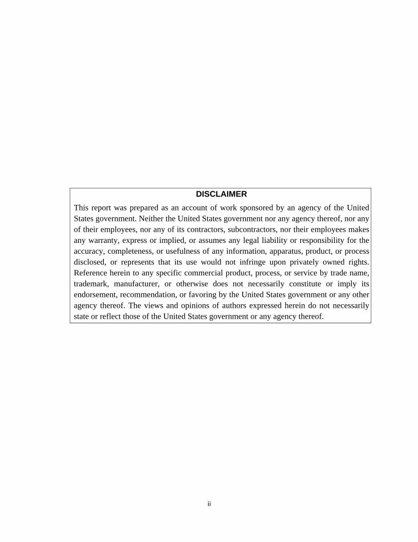
ABSTRACT

Natural gas produced from coal beds (coal-bed methane or CBM) accounts for about 7.5 percent of the total natural gas production in the United States. Along with this gas, water is also brought to the surface. The amount of water produced from most CBM wells is relatively high compared to conventional natural gas wells since coal beds contain many fractures and pores that can contain and transmit large volumes of water. The contribution of CBM to total natural gas production in the United States is expected to increase in the future [1]. As the number of CBM wells increases, the amount of water produced will also increase. Produced water must be treated before reuse and/or disposal. This work aims to improve treatment of produced water by maximizing oxidation of organic compounds present in produced water via ozonation. It is part of a larger project focused on coal-bed methane produced water treatment by means of ozonation, magnetic seeded filtration, and electrosorption. Ozone is a very powerful oxidizing agent used in modern water treatment operations. A treatment process based upon ozonation during a single-pass operation through a gas-liquid reactor was studied. An experimental apparatus consisting of an ozone generator, a counter-flow gas-liquid reactor, and a spectrophotometer was used to monitor the concentration of ozone. Produced water was obtained from coal-bed methane wells in Idaho. The samples were collected after a two-hour interval of treatment. The treated sample showed a significant change in clarity. Then, the treated sample and untreated samples were analyzed for organics content, chloride ion content, and carbonate/bicarbonate content, using a gas chromatograph, an ion selective electrode and a Metrohm Titrino respectively. The results revealed a reduction of one third of the organics, a reduction from 14% to 5% of the chloride ions, and complete elimination of the carbonate/bicarbonate ions.

ARC-2008-D2540-015-04  

iv  

TABLE OF CONTENTS

ABSTRACT ................................................................................................................................... iii

TABLE OF CONTENTS ............................................................................................................... iv

LIST OF FIGURES ........................................................................................................................ v

LIST OF TABLES ......................................................................................................................... vi

1. INTRODUCTION ...................................................................................................................... 1

2. EXECUTIVE SUMMARY ........................................................................................................ 2

3. PROJECT OBJECTIVE ............................................................................................................. 3

4. WATER OZONATION .............................................................................................................. 4

5. POST-TREATMENT ANALYSIS ............................................................................................ 7

5.1 Chloride (Cl-) Ion Analysis ................................................................................................... 7

5.2 Carbonate/Bicarbonate Ion Analysis ................................................................................... 12

5.3 Organic Content Measurement ............................................................................................ 14

6. DISCUSSION OF RESULTS .................................................................................................. 16

7. CONCLUSION AND FUTURE WORK ................................................................................. 17

8. CONTRIBUTION TO OTHER PROJECTS ............................................................................ 18

9. REFERENCES ......................................................................................................................... 19

APPENDIX ................................................................................................................................... 20

 

.

ARC-2008-D2540-015-04  

v  

LIST OF FIGURES

Figure 1. Schematic of the experimental set up for the ozonation experiment in the laboratory. .. 4

Figure 2. Calibration curve for ozonation. ...................................................................................... 5

Figure 3. Laboratory set-up of the ozonation experiment. .............................................................. 6

Figure 4. Samples before and after ozonation. ............................................................................... 6

Figure 5. Ion selective electrode. .................................................................................................... 7

Figure 6. Calibration curve for ISE results. .................................................................................... 8

Figure 7. Results of salinity from previous samples. ...................................................................... 9

Figure 9. Salinity results for produced water samples, trial 1. ..................................................... 11

Figure 10. Salinity results for produced water samples, trial 2. ................................................... 11

Figure 11. Salinity results for produced water samples, average of trials 1 and 2. ...................... 12

Figure 12. Metrohm Titrino. ......................................................................................................... 13

Figure 13. HP 5890 II series gas chromatograph. ......................................................................... 14

Figure 14. GC results for produced water samples. ...................................................................... 15

ARC-2008-D2540-015-04  

vi  

LIST OF TABLES

Table 1. Flow and Absorbance for Calibration Curve .................................................................... 4

Table 2: Flow, Concentration and Absorbance for the Calibration Curve ..................................... 5

Table 3. Cl- Concentration and ISE Results ................................................................................... 7

Table 4. Results of Salinity from Previous Samples ....................................................................... 8

Table 5: Results of Salinity from Previous Samples, Four Trials ................................................... 9

Table 6. Results for Salinity, Trial 1 ............................................................................................. 10

Table 7. Results for Salinity, Trial 2 ............................................................................................. 11

Table 8. Titration Results for HCl , 3 Trials ................................................................................. 12

Table 9. Titration Results for ProducedWater .............................................................................. 13

Table 10. Calculations Results for both treated and untreated produced water samples ............. 13

Table 11. Sample pHs Before and After Acidification ................................................................. 14

ARC-2008-D2540-015-04 

1  

1. INTRODUCTION

Water contained in coal seams must be removed in order to release the methane that is trapped by the groundwater pressure. A series of 1 to 9 production wells are drilled into the coal so that the groundwater can be pumped to the surface to reduce the hydrostatic pressure in the coal seam. The water production from coal-bed methane (CBM) wells typically starts at a high volume but generally falls dramatically over time as the coal seam becomes depressurized in the producing area. Once the fluid pressure is lowered in the coal seam, the methane is released and available for production through the wells. The water produced from CBM wells can vary in quality from very high quality (meeting state and federal drinking water standards) to having very high total dissolved solids (TDS) concentrations (up to180,000 parts per million TDS) which is not suitable for reuse. As a matter of fact, CBM produced water can contain high levels of TDS including bicarbonate/carbonate ions, sodium ions, chloride ions, and organics. Currently, the management of CBM produced water is conducted using various water management practices depending on the quality of the produced water. In areas where the produced water is relatively fresh, the produced water is handled by a wide range of activities including direct discharge, storage in impoundments, livestock watering, irrigation, and dust control. In areas where the water quality is not suitable for direct use, some operators are using treatment prior to discharge. At ORNL, ozonation is being tested as one of those treatments prior to discharge. Ozone is an extremely powerful oxidant that can attack organic materials and convert them to nonhazardous products. It is sparingly soluble in water. The main limitation comes from the low mass transfer rate of ozone from the gas phase to the liquid phase. By use of a glass frit, the effectiveness of ozone as an oxidant can be increased by creating a higher surface area to volume ratio for the contact of ozone with the solution through the generation of smaller bubbles. Smaller bubbles have higher residence times in contactors leading to higher gas volume fractions. This experiment will determine the effectiveness of ozone treatment of CBM produced water.

ARC-2008-D2540-015-04  

2  

2. EXECUTIVE SUMMARY

This research work has been supported by the DOE/FIU Science & Technology Workforce Initiative, an innovative program developed by the US Department of Energy’s Environmental Management (DOE-EM) and Florida International University’s Applied Research Center (FIU-ARC). During the fall semester of 2008, a FIU intern spent 14 weeks doing a fall internship at ORNL’s Nuclear Science and Technology Division under the supervision and guidance of Dr. Costas Tsouris and Dr. Joanna McFarlane. This internship was organized and directed by the Higher Education Research Experience (HERE) and the Oak Ridge Institute for Science and Education (ORISE). The intern’s project was initiated on September 15, 2008, and continued through December 20, 2008, with the objective of treating coal-bed methane produced water using an Ozonation system. The process of Ozonation is the first step of a three step process including magnetic seeded filtration and electrosorption, designed to treat produced water to meet Idaho’s water discharge criteria. The treatment of this water could alleviate the issue of wastewater storage and perhaps the treated water could be reused in very dry areas of the country where it is desperately needed.

ARC-2008-D2540-015-04  

3  

3. PROJECT OBJECTIVE

The objective of this project is to demonstrate that treatment of coal-bed methane (CBM) produced water to discharge criteria via ozonation, magnetic seeded filtration, and electrosorption is possible. The reuse of produced water could alleviate issues of storing the waste water as well as providing clean water in dry areas of the country where it is desperately needed.

ARC-2008-D2540-015-04  

4  

4. WATER OZONATION

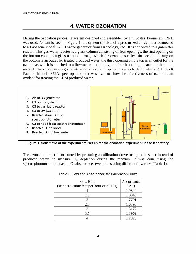
During the ozonation process, a system designed and assembled by Dr. Costas Tsouris at ORNL was used. As can be seen in Figure 1, the system consists of a pressurized air cylinder connected to a Labazone model L-110 ozone generator from Ozonology, Inc. It is connected to a gas-water reactor. This gas-water reactor is a glass column consisting of four openings, the first opening on the bottom contains a glass frit tube through which the ozone gas is fed; the second opening on the bottom is an outlet for treated produced water; the third opening on the top is an outlet for the ozone gas which is attached to a flowmeter, and finally, the fourth opening located on the top is an outlet for ozone gas to go the atmosphere or to the spectrophotometer for analysis. A Hewlett Packard Model 4852A spectrophotometer was used to show the effectiveness of ozone as an oxidant for treating the CBM produced water.

Figure 1. Schematic of the experimental set up for the ozonation experiment in the laboratory.

The ozonation experiment started by preparing a calibration curve, using pure water instead of produced water, to measure O3 depletion during the reaction. It was done using the spectrophotometer to measure O3 absorbance seven times using different flow rates (Table 1).

Table 1. Flow and Absorbance for Calibration Curve 

Flow Rate (standard cubic feet per hour or SCFH)

Absorbance (Au)

1 1.9844 1.5 1.8845 2 1.7701

2.5 1.6395 3 1.5177

3.5 1.3969 4 1.2926

 

1. Air to O3 generator  2. O3 out to system  3. O3 to gas liquid reactor 4. O3 to UV (O3 Trap) 5. Reacted stream O3 to 

spectrophotometer  6. O3 to hood from spectrophotometer 7. Reacted O3 to hood  8. Reacted O3 to flow meter  

ARC-2008-D2540-015-04  

5  

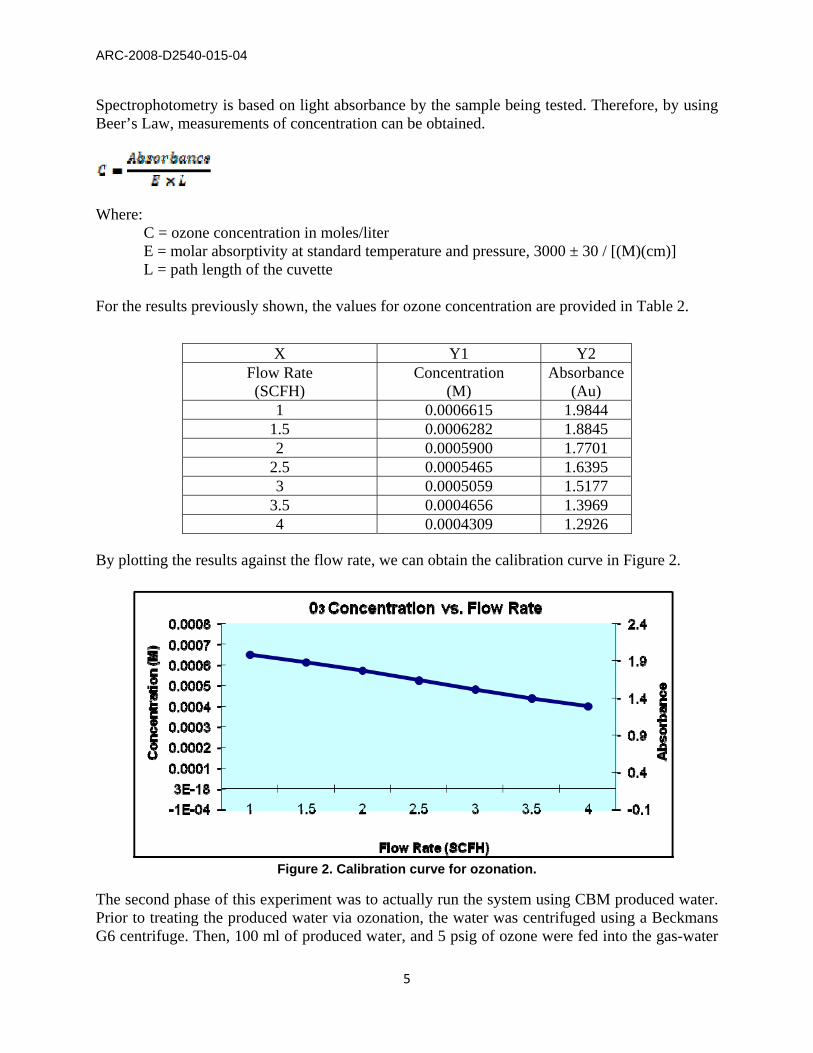
Spectrophotometry is based on light absorbance by the sample being tested. Therefore, by using Beer’s Law, measurements of concentration can be obtained.

Where:

C = ozone concentration in moles/liter E = molar absorptivity at standard temperature and pressure, 3000 ± 30 / [(M)(cm)] L = path length of the cuvette

For the results previously shown, the values for ozone concentration are provided in Table 2.

X Y1 Y2 Flow Rate (SCFH)

Concentration (M)

Absorbance (Au)

1 0.0006615 1.9844 1.5 0.0006282 1.8845 2 0.0005900 1.7701

2.5 0.0005465 1.6395 3 0.0005059 1.5177

3.5 0.0004656 1.3969 4 0.0004309 1.2926

By plotting the results against the flow rate, we can obtain the calibration curve in Figure 2.

Figure 2. Calibration curve for ozonation.

The second phase of this experiment was to actually run the system using CBM produced water. Prior to treating the produced water via ozonation, the water was centrifuged using a Beckmans G6 centrifuge. Then, 100 ml of produced water, and 5 psig of ozone were fed into the gas-water

ARC-2008-D2540-015-04  

6  

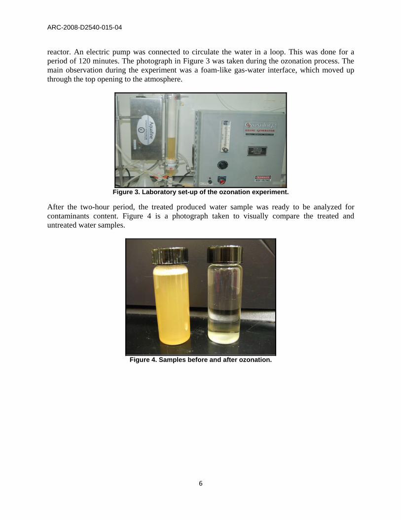
reactor. An electric pump was connected to circulate the water in a loop. This was done for a period of 120 minutes. The photograph in Figure 3 was taken during the ozonation process. The main observation during the experiment was a foam-like gas-water interface, which moved up through the top opening to the atmosphere.

Figure 3. Laboratory set-up of the ozonation experiment.

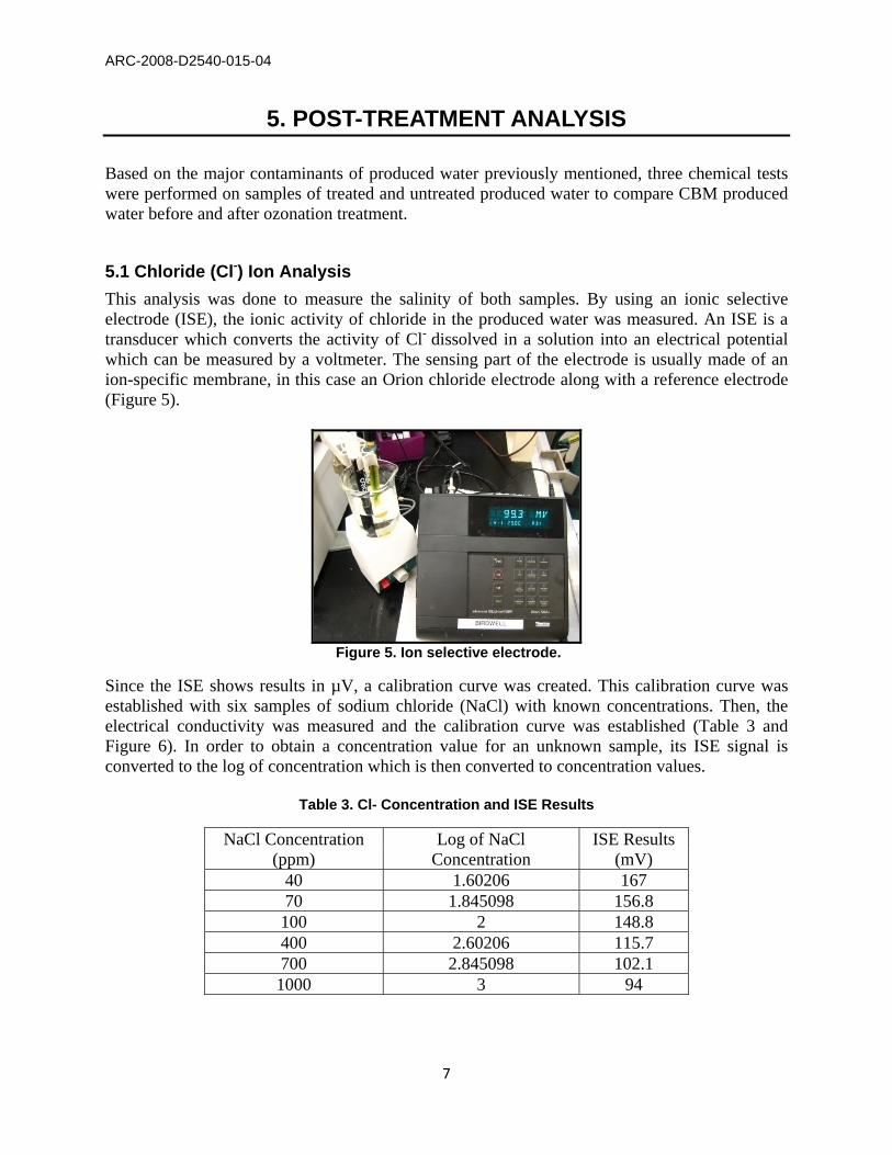
After the two-hour period, the treated produced water sample was ready to be analyzed for contaminants content. Figure 4 is a photograph taken to visually compare the treated and untreated water samples.

Figure 4. Samples before and after ozonation.

ARC-2008-D2540-015-04  

7  

5. POST-TREATMENT ANALYSIS

Based on the major contaminants of produced water previously mentioned, three chemical tests were performed on samples of treated and untreated produced water to compare CBM produced water before and after ozonation treatment.

5.1 Chloride (Cl-) Ion Analysis

This analysis was done to measure the salinity of both samples. By using an ionic selective electrode (ISE), the ionic activity of chloride in the produced water was measured. An ISE is a transducer which converts the activity of Cl- dissolved in a solution into an electrical potential which can be measured by a voltmeter. The sensing part of the electrode is usually made of an ion-specific membrane, in this case an Orion chloride electrode along with a reference electrode (Figure 5).

Figure 5. Ion selective electrode.

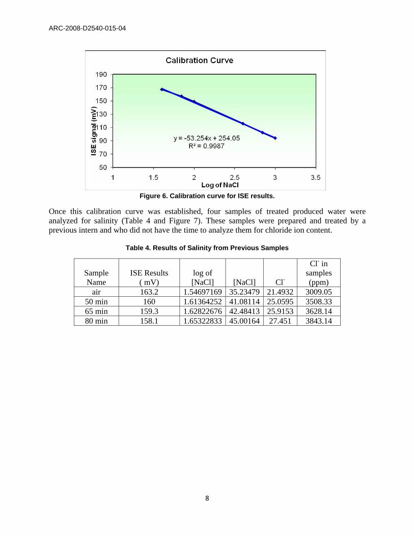
Since the ISE shows results in µV, a calibration curve was created. This calibration curve was established with six samples of sodium chloride (NaCl) with known concentrations. Then, the electrical conductivity was measured and the calibration curve was established (Table 3 and Figure 6). In order to obtain a concentration value for an unknown sample, its ISE signal is converted to the log of concentration which is then converted to concentration values.

Table 3. Cl- Concentration and ISE Results

NaCl Concentration (ppm)

Log of NaCl Concentration

ISE Results (mV)

40 1.60206 167 70 1.845098 156.8 100 2 148.8 400 2.60206 115.7 700 2.845098 102.1 1000 3 94

ARC-2008-D2540-015-04  

8  

Figure 6. Calibration curve for ISE results.

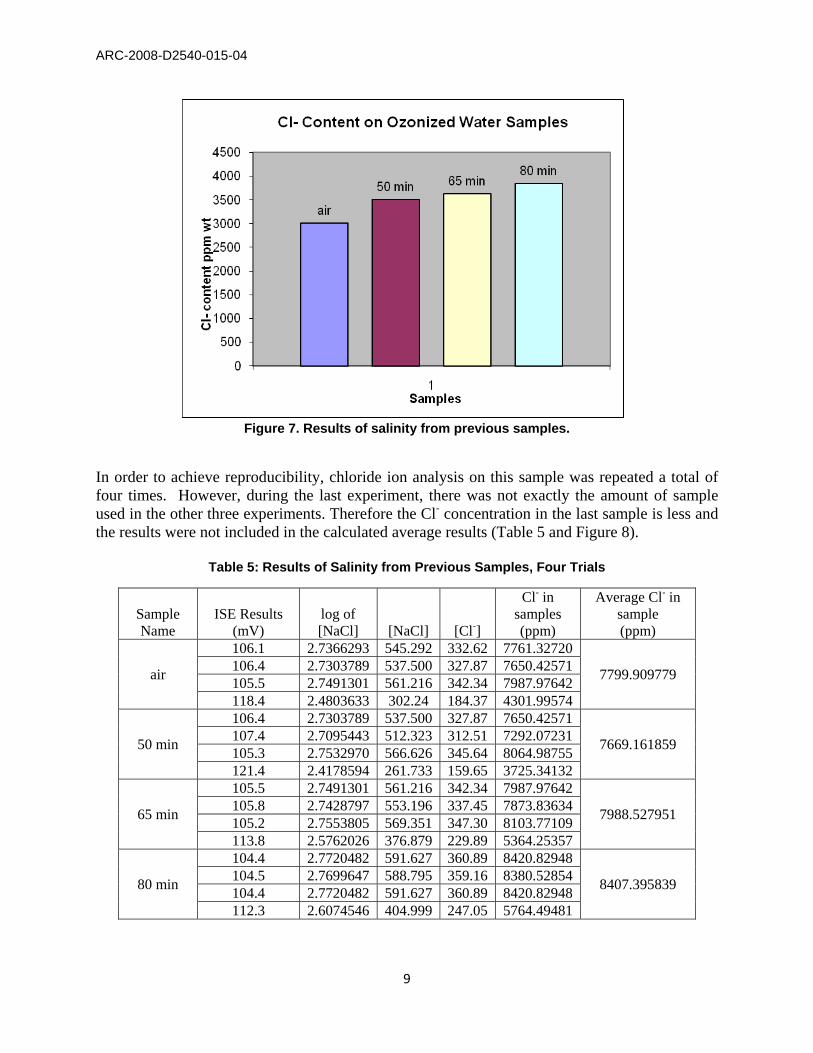
Once this calibration curve was established, four samples of treated produced water were analyzed for salinity (Table 4 and Figure 7). These samples were prepared and treated by a previous intern and who did not have the time to analyze them for chloride ion content.

Table 4. Results of Salinity from Previous Samples

Sample Name

ISE Results ( mV)

log of [NaCl] [NaCl] Cl-

Cl- in samples (ppm)

air 163.2 1.54697169 35.23479 21.4932 3009.05 50 min 160 1.61364252 41.08114 25.0595 3508.33 65 min 159.3 1.62822676 42.48413 25.9153 3628.14 80 min 158.1 1.65322833 45.00164 27.451 3843.14

ARC-2008-D2540-015-04  

9  

Figure 7. Results of salinity from previous samples.

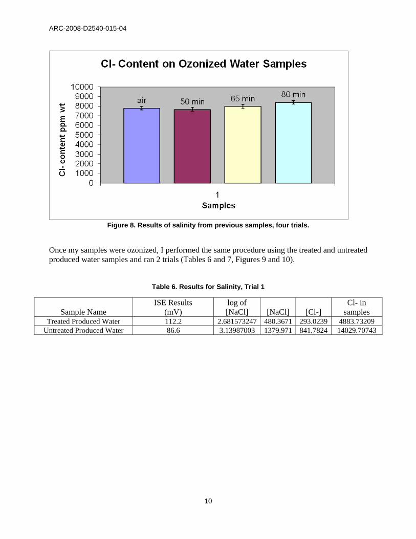
In order to achieve reproducibility, chloride ion analysis on this sample was repeated a total of four times. However, during the last experiment, there was not exactly the amount of sample used in the other three experiments. Therefore the Cl- concentration in the last sample is less and the results were not included in the calculated average results (Table 5 and Figure 8).

Table 5: Results of Salinity from Previous Samples, Four Trials

Sample Name

ISE Results (mV)

log of [NaCl] [NaCl] [Cl-]

Cl- in samples (ppm)

Average Cl- in sample (ppm)

air

106.1 2.7366293 545.292 332.62 7761.32720

7799.909779 106.4 2.7303789 537.500 327.87 7650.42571 105.5 2.7491301 561.216 342.34 7987.97642 118.4 2.4803633 302.24 184.37 4301.99574

50 min

106.4 2.7303789 537.500 327.87 7650.42571

7669.161859 107.4 2.7095443 512.323 312.51 7292.07231 105.3 2.7532970 566.626 345.64 8064.98755 121.4 2.4178594 261.733 159.65 3725.34132

65 min

105.5 2.7491301 561.216 342.34 7987.97642

7988.527951 105.8 2.7428797 553.196 337.45 7873.83634 105.2 2.7553805 569.351 347.30 8103.77109 113.8 2.5762026 376.879 229.89 5364.25357

80 min

104.4 2.7720482 591.627 360.89 8420.82948

8407.395839 104.5 2.7699647 588.795 359.16 8380.52854 104.4 2.7720482 591.627 360.89 8420.82948 112.3 2.6074546 404.999 247.05 5764.49481

ARC-2008-D2540-015-04  

10  

Figure 8. Results of salinity from previous samples, four trials.

Once my samples were ozonized, I performed the same procedure using the treated and untreated produced water samples and ran 2 trials (Tables 6 and 7, Figures 9 and 10).

Table 6. Results for Salinity, Trial 1

Sample Name ISE Results

(mV) log of [NaCl] [NaCl] [Cl-]

Cl- in samples

Treated Produced Water 112.2 2.681573247 480.3671 293.0239 4883.73209 Untreated Produced Water 86.6 3.13987003 1379.971 841.7824 14029.70743

ARC-2008-D2540-015-04  

11  

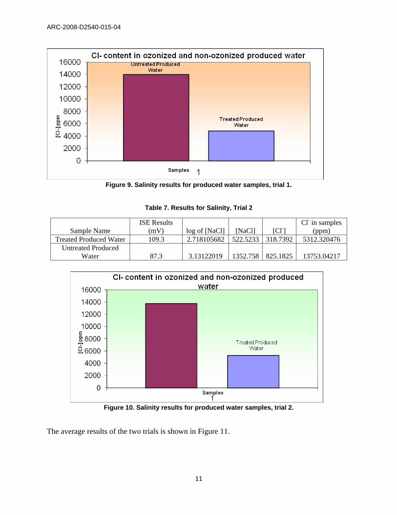
Figure 9. Salinity results for produced water samples, trial 1.

Table 7. Results for Salinity, Trial 2

Sample Name ISE Results

(mV) log of [NaCl] [NaCl] [Cl-] Cl- in samples

(ppm) Treated Produced Water 109.3 2.718105682 522.5233 318.7392 5312.320476

Untreated Produced Water 87.3 3.13122019 1352.758 825.1825 13753.04217

Figure 10. Salinity results for produced water samples, trial 2.

The average results of the two trials is shown in Figure 11.

ARC-2008-D2540-015-04  

12  

Figure 11. Salinity results for produced water samples, average of trials 1 and 2.

5.2 Carbonate/Bicarbonate Ion Analysis

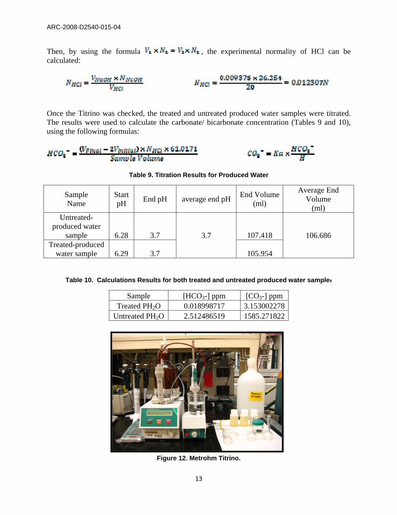
Carbonate/bicarbonate ion analysis was performed by titration. Titration is a common laboratory method of quantitative chemical analysis that is used to determine the unknown concentration of a known reactant. A reagent, called the titrant, of known concentration (a standard solution) and volume is used to react with a solution of the analyte or titrand, whose concentration is not known. In this case, I used a Metrohm Titrino, which is an electronic titrator (Figure 12). The procedure “Measurements for Carbonate and Bicarbonate in Produced Water” (Appendix) was followed during this experiment. Basically, two solutions were prepared: 0.01N NaoH and 0.01N HCl. The HCl solution was then used as the titrand and the NaOH as the titrant, for 3 trials, to check the Titrino. Table 8 summarizes the end pHs and volumes of these three runs.

Table 8. Titration Results for HCl , 3 Trials

Trial Start pH End pH Average End

pH End Volume

(ml) Average End Volume

(ml) 1 2.02 7.27

7.233333333 26.729

26.254 2 2.08 7.21 27.342 3 2.03 7.22 24.691

ARC-2008-D2540-015-04  

13  

Then, by using the formula , the experimental normality of HCl can be calculated:

Once the Titrino was checked, the treated and untreated produced water samples were titrated. The results were used to calculate the carbonate/ bicarbonate concentration (Tables 9 and 10), using the following formulas:

Table 9. Titration Results for Produced Water

Sample Name

Start pH

End pH average end pH End Volume

(ml)

Average End Volume

(ml) Untreated-

produced water sample 6.28 3.7 3.7 107.418 106.686

Treated-produced water sample 6.29 3.7 105.954

Table 10. Calculations Results for both treated and untreated produced water samples

Sample [HCO3-] ppm [CO3-] ppm Treated PH2O 0.018998717 3.153002278

Untreated PH2O 2.512486519 1585.271822

Figure 12. Metrohm Titrino.

ARC-2008-D2540-015-04  

14  

5.3 Organic Content Measurement

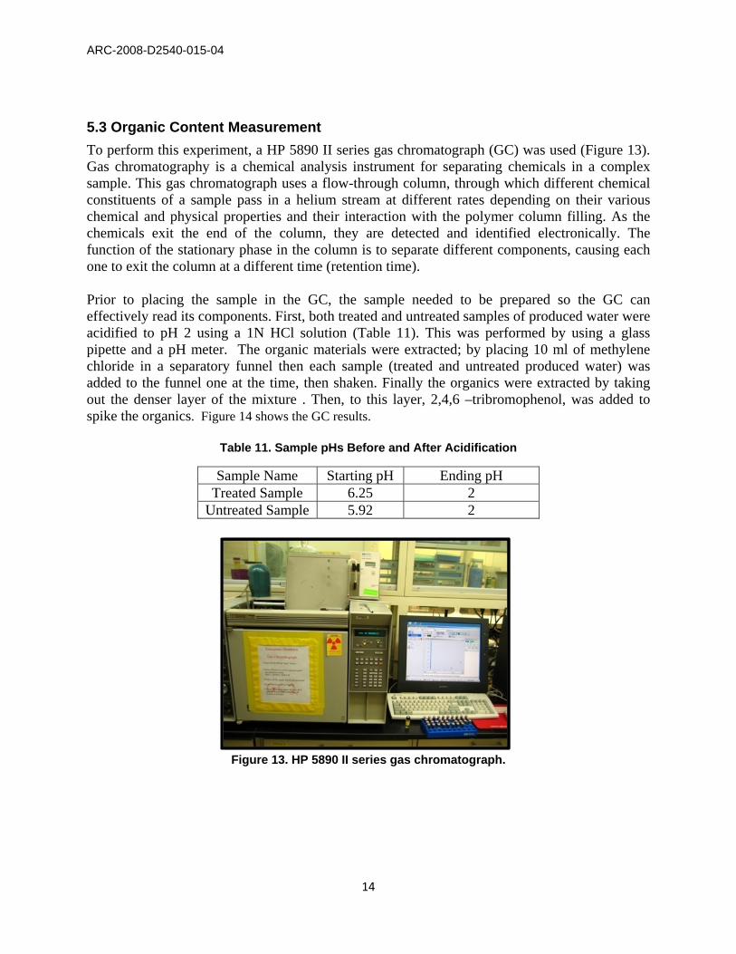
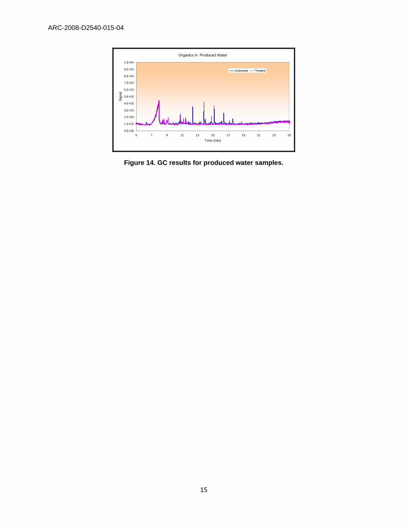
To perform this experiment, a HP 5890 II series gas chromatograph (GC) was used (Figure 13). Gas chromatography is a chemical analysis instrument for separating chemicals in a complex sample. This gas chromatograph uses a flow-through column, through which different chemical constituents of a sample pass in a helium stream at different rates depending on their various chemical and physical properties and their interaction with the polymer column filling. As the chemicals exit the end of the column, they are detected and identified electronically. The function of the stationary phase in the column is to separate different components, causing each one to exit the column at a different time (retention time). Prior to placing the sample in the GC, the sample needed to be prepared so the GC can effectively read its components. First, both treated and untreated samples of produced water were acidified to pH 2 using a 1N HCl solution (Table 11). This was performed by using a glass pipette and a pH meter. The organic materials were extracted; by placing 10 ml of methylene chloride in a separatory funnel then each sample (treated and untreated produced water) was added to the funnel one at the time, then shaken. Finally the organics were extracted by taking out the denser layer of the mixture . Then, to this layer, 2,4,6 –tribromophenol, was added to spike the organics. Figure 14 shows the GC results.

Table 11. Sample pHs Before and After Acidification

Sample Name Starting pH Ending pH Treated Sample 6.25 2

Untreated Sample 5.92 2

Figure 13. HP 5890 II series gas chromatograph.

ARC-2008-D2540-015-04  

15  

Organics in Produced Water

0.E+00

1.E+03

2.E+03

3.E+03

4.E+03

5.E+03

6.E+03

7.E+03

8.E+03

9.E+03

1.E+04

5 7 9 11 13 15 17 19 21 23 25

Time (min)

Sig

nal

Untreated Treated

Figure 14. GC results for produced water samples.

ARC-2008-D2540-015-04  

16  

6. DISCUSSION OF RESULTS

The objective of the experiments was to determine the affect of ozonation on decreasing the major contaminants of CBM produced water: chloride ions, carbonate/bicarbonate ions and organics. The first test measured ionic interaction using an ion selective electrode. The results of ISE are shown in Figures 9 and 10. The concentration of chloride ions in the samples was reduced from 14,000 ppm in the untreated produced water sample to 5,000 ppm in the treated produced water sample. This represents a decrease from 14% salinity to 5%. According to the practical salinity scale (PSS) the salinity of the samples went from saline water, which is equivalent to sea water, to brackish water, which has a higher salinity than fresh water but a lower salinity than saline water. The second test, carbonate/bicarbonate ion analysis, reflected a decrease in these ions to about 0%. Ozonation results in the breaking of double bonds in compounds so most likely, the ozonation treatment of the produced water broke the double bonds of the carbonate/bicarbonate ions. Lastly, the organic content results reflected a reduction or elimination of one third of the organic content. This portion encompasses the longer-chain aliphatic hydrocarbons, and the n-alkanes (C12 to C19). The visual results indicated a significant change in color as shown in Figure 5. Prior to ozonation, the CBM produced water looked dark and dense. After ozonation, the treated CBM produced water had a clear appearance.

ARC-2008-D2540-015-04  

17  

7. CONCLUSION AND FUTURE WORK

The results of this experiment were very successful. Contaminants in the CBM produced water were eliminated to a great extent. Ozonation is an excellent approach to the treatment of CBM produced water to eliminate the major contaminants: carbonate/bicarbonate ions, chloride ions, and various organics. Rates of elimination of these contaminants were very satisfactory. The samples need further analyses by inductively coupled plasma mass spectrometry (ICP-MS) to detect the presence of other minerals. In addition, the samples cannot be considered for reuse yet as they still need to undergo additional treatment via electrosorption and magnetic seeded filtration, in addition to post treatment analysis.

ARC-2008-D2540-015-04  

18  

8. CONTRIBUTION TO OTHER PROJECTS

During this internship, I also had the opportunity to collaborate in other two projects. The first project focused in the analysis of biodiesel production kinetics for a biodiesel production company, NuEnergy, located in the tri-cities area of Tennessee. The main objective of this project was to find the residence time for biodiesel production. I had the opportunity to participate in several biodiesel production mimicking runs where twelve samples were obtained. After these samples were obtained, they were prepared for the gas chromatograph. I also had the opportunity to visit NuEnergy, see biodiesel production on a large scale, and witness the functioning of such a plant. The second project was related to the study of surface interactions of radioactive particles and their transport and deposition. In order to perform this study, an atomic force microscope (AFM) was used. The AFM, or scanning force microscope (SFM), is a very high-resolution type of scanning probe microscope, with demonstrated resolution of fractions of a nanometer. The AFM is one of the foremost tools for imaging, measuring and manipulating matter at the nano scale. The information is gathered with a mechanical probe. Piezoelectric elements that facilitate tiny but accurate and precise movements on command enable the very precise scanning.

ARC-2008-D2540-015-04  

19  

9. REFERENCES

 [1] ALL Consulting, Handbook on Coal Bed Methane Produced Water: Management and Beneficial Use Alternatives. Tulsa, Oklahoma. 2003.

[2] American Public Health Association, American Water Works Association, Water Pollution

Control Federation. STANDARD METHODS :For the Examination of Water and Wastewater . Washington ,DC: APHA, AWWA, WPCF, 1985.

ARC-2008-D2540-015-04  

20  

APPENDIX

Measurements for Carbonate and Bicarbonate in Produced Water A Metrohm 717 DMS Titrino automatic titrator is used to determine the pH and the hydroxide/bicarbonate/carbonate content of produced water samples (Franson 1992). Use 60 mL sample (3x20 aliquots) of produced water Standard solutions: Use degassed DI (boil for 15 minutes and then cool, pH>6) standardization of NaOH (0.01 N) dissolve 0.4 g NaOH in 1 L degassed DI Prepare KHC8H4O4 (potassium hydrogen phthalate, CAS 877-24-7) solution by crushing 15-20 g KHC8H4O4 and dry at 120 °C for 2 h. Let cool in a dessicator. Weigh 1g KHC8H4O4 and make up in 1 L volumetric flask to ~0.005N. Titrate 40 mL KHC8H4O4 solution using NaOH. Inflection point should be around pH 8.7 – repeat 3 times for statistics Prepare HCl (0.01 N) by diluting 5 N HCl (2 mL stock in 1 L solution) Titrate 40 mL HCl with standardized 0.01 N NaOH prepared in step 1. Repeat three times for statistics. The instrument is calibrated with two NIST-traceable buffer solutions (pH 7 and pH 10, respectively). The temperature of the solution is entered digitally before the pH of the sample is measured. The OH, CO3

2, and HCO3 concentrations are determined by titrating 20 mL of

produced water with standard 0.01 N HCl. End points are measured at pH 8.3 (i.e., volume end point A) and 3.7 (i.e., volume end point B), which are then entered into the following calculations: Calculations If 2A > B, the solution contains OH and CO3

2,

(2A – B) normality of HCl 17.0073/(sample volume) = ppm OH,

2(B – A) normality of HCl 30.0046 /(sample volume, mL) = ppm CO32.

If B > 2A, the solution contains CO32 and HCO3

,

2A normality of HCl 30.0046 /(sample volume, mL) = ppm CO32,

(B – 2A) normality of HCl 61.0171 /(sample volume, mL) = ppm HCO3.

Total alkalinity is determined from the total volume of acid required to achieve a pH of 3.7. It is calculated as:

(A + B) normality of HCl 1000 = Alkalinity to pH 3.7, mg CaCO3/L sample volume, mL