Embed Size (px)
Citation preview
182
American Economic Journal: Microeconomics 2013, 6(1): 182–204 http://dx.doi.org/10.1257/mic.6.1.182
Coalition Formation in a Legislative Voting Game†
By Nels Christiansen, Sotiris Georganas, and John H. Kagel*
We experimentally investigate the Jackson and Moselle (2002) model where legislators bargain over policy proposals and the allocation of private goods. Key comparative static predictions of the model hold with the introduction of private goods, including “strange bedfel-low” coalitions. Private goods help to secure legislative compromise and increase the likelihood of proposals passing, an outcome not predicted by the theory but a staple of the applied political economy literature. Coalition formation is better characterized by an “efficient equal split” between coalition partners than the subgame perfect equilibrium prediction, which has implications for stable political party formation. (JEL C78, D72, H41)
Legislative bargaining often consists of dealing with public policy issues with strong ideological elements (e.g., bank bailouts or abortion rights) along with
purely distributive (private good) allocations. The present paper experimentally investigates the Jackson and Moselle (2002) model of legislative bargaining over public policy issues including the role private goods play in policymaking, the nature of winning coalitions, and the stability of political parties. The model simplifies the bargaining process to one in which legislators bargain over a single dimensional public policy issue, possibly representing familiar distinctions between liberal and conservative policy positions, and the distribution of private goods across legislative constituencies. Legislators are assumed to have single peaked preferences over the policy issue with differential “costs” deviating from these preferences. In contrast, legislators have uniform preferences over distributive goods, with each legislator preferring larger amounts for his constituency. The introduction of private goods (aka pork) into the legislative bargaining process is predicted to open up the possi-bility of “strange bedfellow” coalitions consisting of legislators to the left and right of center, an outcome reliably observed in the data. Private goods may also increase total welfare net of their cost. Although the latter is not predicted in our experimental
* Christiansen: Department of Economics, Trinity University, One Trinity Place, San Antonio, TX 78212 (e-mail: [email protected]); Georganas: Department of Economics, Royal Holloway, University of London, 206 McRae, Egham, Surrey, TW20 0EX, UK (e-mail: [email protected]); Kagel: Department of Economics, Ohio State University, 10 Arps Hall, 1945 N High Street, Columbus, OH 43210 (e-mail: [email protected]). We thank Guillaume Fréchette, Matthew Jackson, and two anonymous referees for helpful comments on an earlier version of this paper. Matthew Jones and Peter McGee provided valuable research assistance. We alone are responsible for any errors and omissions. Support for this research was provided by National Science Foundation grants SES 0924764 and SES 122646, and the Ohio State University. Any opinions, findings, and conclusions or recommendations in this material are those of the authors and do not necessarily reflect the views of the National Science Foundation.
† Go to http://dx.doi.org/10.1257/mic.6.1.182 to visit the article page for additional materials and author disclo-sure statement(s) or to comment in the online discussion forum.
VoL. 6 No. 1 183christiansen et al.: legislative bargaining
design, we find that net welfare increases as fewer relatively inefficient policies pass. We also find that the introduction of distributive goods into the bargaining pro-cess increases the likelihood of proposals passing. Although this too is not predicted in the theory, it is consistent with field data showing that legislative compromise is easier with distributive goods available to grease the wheels (Evans 2004).
Our experiment employs the simplest possible setting with three legislators. We focus on the comparative static predictions of the model with and without the pres-ence of distributive goods for forging legislative compromise. In the experimental treatment reported on in the body of the paper, the total value of the legislators’ equilibrium payoffs remains constant between bargaining over the public policy issue alone and bargaining over the public policy issue in conjunction with private goods (net of the cost of the private goods). Key aggregate comparative static pre-dictions of the model are satisfied as the introduction of private goods shifts the average location of the public policy issue significantly from near the median legis-lator’s preferred outcome to a location that is closer to the preferred outcome of the extreme legislator who cares the most about the issue (a result of strange bedfellow coalitions). Private goods also increase the variance around the mean public policy outcome, as predicted within the theory.
The total value of players’ payoffs increases modestly, but significantly, with the introduction of distributive goods after accounting for their cost. At a more micro level most, but far from all, players with extreme public policy preferences effec-tively use distributive goods to move the policy outcome closer to their preferred position. However, the more subtle prediction in which the median legislator forms a coalition with the legislator with the more extreme policy preferences fails, as most coalitions proposed by the median legislator are formed with the player with closer policy preferences. This, in turn, has important implications for what constitute via-ble political parties, resulting in only one, not two, viable parties as the Jackson and Moselle (2002)—henceforth, JM—model predicts under the stationary subgame perfect equilibrium outcome.
The outline of the paper is as follows: Section I briefly reviews results from ear-lier extensive form legislative bargaining experiments in the Baron and Ferejohn (1989) tradition which provides the springboard for the present research. Section II outlines the predictions of the JM model for the parameter specification employed in the text. Section III describes the experimental procedures, with Section IV reporting the experimental results, along with the implications of these results for what constitute stable political parties. Section V concludes with a brief summary of the results and their similarities and differences with other legislative bargain-ing experiments. There is a rather long online Appendix to the paper reporting the motivation for, as well as outcomes of, a second set of treatment parameters. These results are relegated to an online Appendix as (i) the main results are quite similar to those reported in the text, but (ii) the predictions of the model along with the data analysis are complicated by the presence of a mixed strategy equilibrium. There will be a brief discussion of these results in Section IV where they help shape our understanding of the main treatment outcomes. Readers with particular interests in legislative bargaining models of the sort studied here are encouraged to read the online Appendix.
184 AMEriCAN ECoNoMiC JourNAL: MiCroECoNoMiCs fEBruAry 2014
I. Previous Research on Multilateral Bargaining in the Shadow of a Voting Rule1
The present paper adds to the growing experimental literature on legislative bargaining in games with a fixed extensive form. The inspiration for most of this research is the Baron and Ferejohn (1989)—henceforth, BF—bargaining model. In the simplest version of the model, a committee of size n (where n is an odd number) must decide over an allocation of money between the committee members with one of the members “recognized” (typically selected at random) to make a proposed allocation that is voted up or down. The game ends when a proposal is accepted by a majority of members with the proposed allocation binding. If the proposal is rejected, there is a new call for proposals, one of which is again randomly selected to be voted on, with this process continuing indefinitely until a proposal is accepted. There are many variations of this basic game generated by changing the recognition rule (unequal recognition probabilities) or the voting rule (super majority or veto players), introducing time preferences (the amount of money available shrinks by a factor δ ∈ [0, 1] if a proposal is rejected), having a terminal period T, allowing amendments to the proposed allocation, specifying a status quo in case no proposal is accepted, etc.
Most past experiments deal with divide the dollar games in which committee members bargain over the allocation of private goods between legislative districts (McKelvey 1991; Diermeier and Morton 2005; Fréchette, Kagel, and Morelli 2005a, b).2 Results from divide the dollar games close in structure to the game reported on below (an infinite horizon game with δ = 1) are generally consistent with the comparative static predictions of the model, but with significant deviations from the model’s point predictions as: (i) the majority of games end without delay, as the theory predicts, with this frequency growing with experience; (ii) the major-ity of games involve minimum winning coalitions (MWCs) as the theory predicts, with their frequency growing with experience; and (iii) there is significant proposer power, but it is typically far from the level predicted under the stationary subgame perfect equilibrium (SSPE) prediction. Closely related to (iii) is that allocations with proposer power at, or near, the level predicted under the SSPE would be voted down with near certainty.3 As predicted, proposer power is diminished by allow-ing amendments to proposals (Frécehtte, Kagel, and Lehrer 2003) and, for nonveto players, when a veto player is present (Kagel, Sung, and Winter 2010). Further, proposer power increases with impatience (δ < 1) (Fréchette, Kagel, and Morelli 2005a) and for veto players compared to games without veto players (Kagel, Sung, and Winter 2010).4
1 This review closely follows the one offered in Palfrey (forthcoming). For details, as well as a review of the earlier legislative bargaining literature, see his survey.
2 To name but a few of the many papers in this area. Also see Diermeir and Gailmard (2006); Fréchette, Kagel, and Lehrer (2003); Fréchette (2009).
3 See Fréchette, Kagel, and Morelli (2005a, b, c). Results from dynamic divide the dollar games with an endog-enous status quo yield comparable results in that MWCs are observed about as much as in the BF game, with more equal player shares than predicted and with proposals usually being accepted (Battaglini and Palfrey 2012).
4 For finite horizon games see Diermeier and Morton (2005) (games with a maximum of five rounds) and Diermeier and Gilmard (2006) (one round games).
VoL. 6 No. 1 185christiansen et al.: legislative bargaining
Extensions of the infinite horizon BF game to include choosing over public and private goods (Volden and Wiseman 2007) predict that when all players have the same value for the public good, and the marginal utility from the private good is not too large, only the proposer obtains private goods in the SSPE, with proposers using public goods to obtain willing coalition partners. Further, in the mixed region where both public and private goods are provided, as the relative value of public good decreases, the model predicts, somewhat counterintuitively, that a larger bud-get share will be allocated to the public good. Fréchette, Kagel, and Morelli (2012) show that the experimental data are largely consistent with this first prediction, as within the mixed region allocations converge toward private goods being provided exclusively to the proposer. However, the public good’s share of the budget decreases as the value of the public good decreases, contrary to the model’s prediction.5
Christiansen (2010) experimentally investigates a version of the Volden-Wiseman model where two different blocks of legislators have different (but constant) mar-ginal rates of substitution between public and private goods. Depending on the pro-poser’s type, either private goods or public goods will be used to secure legislative compromise, and to form a minimum winning coalition, with both of these out-comes observed in the data. Several unpredicted results are reported as well, includ-ing clear breakdowns of the stationarity assumption when private good preferring types propose to take too much for themselves, as they get significantly smaller payoffs following rejection of their proposed allocations.
In the Volden-Wiseman (VM) version of the BF legislative bargaining model pork and public goods are funded from a common budget with the model focusing on the tradeoffs in the budget allocation process between public and private goods. The public component of the JM model consists of either a public policy proposal with an ideological component (e.g., limits on abortion rights or gay marriage), which the VM model is not equipped to deal with, or a proposal to fund the public good as in the VM model. In terms of funding levels for the public good, funds for private goods are exogenous in the JM model, so one can think of the trade-off in the budget process as between funding a given public good and funding other pub-lic goods, or funding a given public good but one that also has local benefits (e.g., the location of a military base has additional economic benefits largely confined to the legislative district in which it is located). The downside to this is that there is no direct mechanism for investigating the budgetary tradeoffs between public and private goods as in the VW model. However, the JM model allows one to ask ques-tions not explored in the previous literature regarding an important class of public policy/public good issues, including how the introduction of private goods moves the policy location chosen away from the median’s ideal point, how private goods impact efficiency, and how private goods can get legislators with opposing ideolo-gies to work together.
5 Battaglini, Nunnari, and Palfrey (2012) investigate a dynamic legislative bargaining model with durable pub-lic goods in which all players have the same utility function which is linear in the private good with an additively separable concave utility function for the public good.
186 AMEriCAN ECoNoMiC JourNAL: MiCroECoNoMiCs fEBruAry 2014
II. The Legislative Bargaining Model
The JM model employs a bargaining structure that is the same as the basic BF structure outlined in the previous section: In our case an infinite horizon game with n = 3, with proposers chosen randomly (with equal probability), proposals voted up or down without the possibility of amendments, and δ = 1.6 A proposal is a vec-tor ( y, x1, x2, x3) consisting of a public policy proposal y and a distributive proposal x1, x2, x3. The set of feasible public policy proposals is [0, y ] where y ∈ [0, 100] and the set of private allocations is such that x i ≥ 0 for each i with ∑ x i ≤ X where X ≥ 0. When y = 0, the model simplifies to the BF divide the dollar game where X is the total amount of pure private goods to be distributed among legislative districts. At the other extreme, when X = 0 the model reduces to a median voter game with y capturing the public policy decision.
Each legislator has preferences over decisions that depend on y and x i , his or her share of the private good. Legislator i’s utility function u i ( y, x i ) is nonnegative, continuous, and strictly increasing in x i for every y ∈ y. Preferences over the public policy are separable from the distributive decision for each i and u i is single peaked in y, with the ideal point noted as y i
∗ .Legislators observe all proposals voted on, and the outcome of those votes, prior
to making any new proposals. As in the standard BF game, the full set of Nash equilibria for this game is large, with some equilibria involving complex, contingent strategies. As is commonly the case we focus on the stationary subgame perfect equilibrium (SSPE) for theoretical predictions.
In games where X = 0 and δ = 1, the preferred point of the median legislator, y med
∗ , is proposed and eventually approved with probability 1 in any SSPE. The intuition here is that a proposal that is not at the median legislator’s ideal point will not win approval since the median legislator, and the legislator to the other side of the proposed y, can wait and do better. In games where X > 0 and y > 0 there is a positive probability that a proposal wins approval with a coalition that excludes the median legislator. That is, there is a positive probability that a proposal wins approval which includes members of a disjoint coalition. The next section charac-terizes the possible SSPE outcomes under our experimental treatment conditions.
III. Experimental Design and Procedures
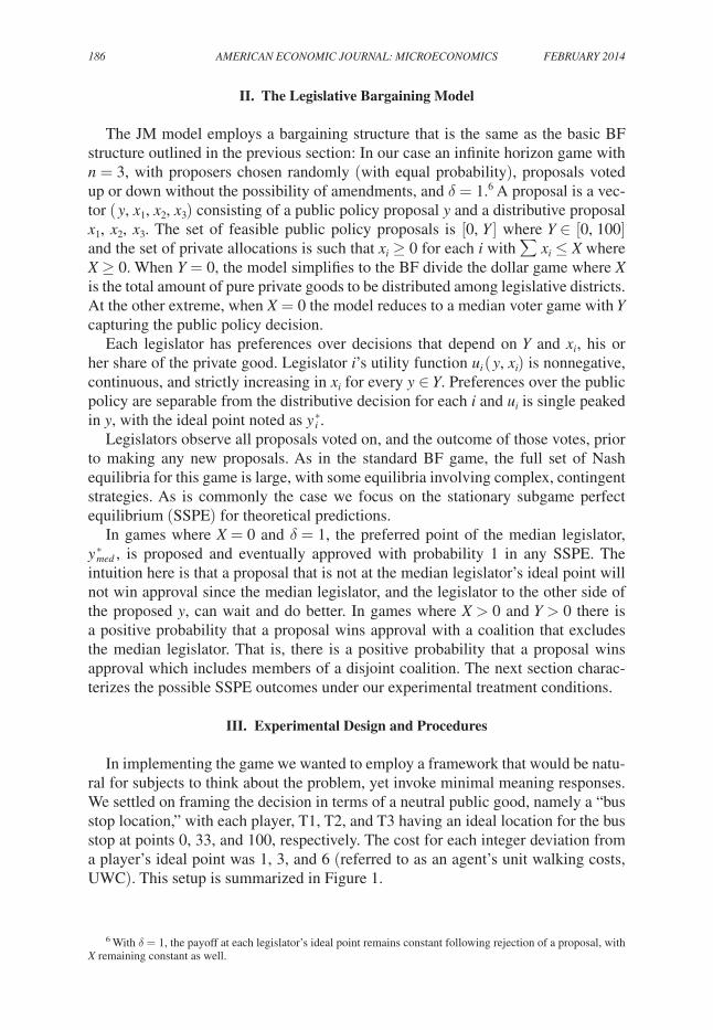
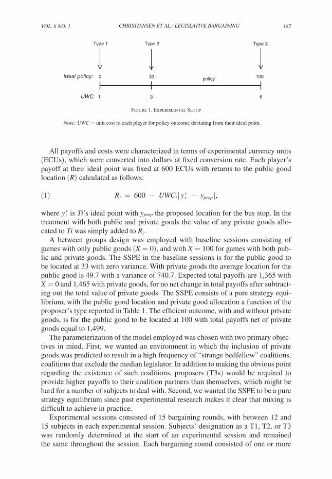
In implementing the game we wanted to employ a framework that would be natu-ral for subjects to think about the problem, yet invoke minimal meaning responses. We settled on framing the decision in terms of a neutral public good, namely a “bus stop location,” with each player, T1, T2, and T3 having an ideal location for the bus stop at points 0, 33, and 100, respectively. The cost for each integer deviation from a player’s ideal point was 1, 3, and 6 (referred to as an agent’s unit walking costs, UWC). This setup is summarized in Figure 1.
6 With δ = 1, the payoff at each legislator’s ideal point remains constant following rejection of a proposal, with X remaining constant as well.
Vol. 6 No. 1 187christiansen et al.: legislative bargaining
All payoffs and costs were characterized in terms of experimental currency units (ECUs), which were converted into dollars at fixed conversion rate. Each player’s payoff at their ideal point was fixed at 600 ECUs with returns to the public good location (R) calculated as follows:
(1) R i = 600 − UW C i | y i ∗ − y prop |,
where y i ∗ is Ti’s ideal point with y prop the proposed location for the bus stop. In the
treatment with both public and private goods the value of any private goods allo-cated to Ti was simply added to R i .
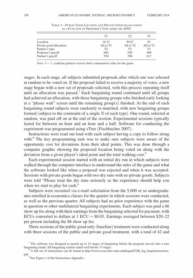
A between groups design was employed with baseline sessions consisting of games with only public goods (X = 0), and with X = 100 for games with both pub-lic and private goods. The SSPE in the baseline sessions is for the public good to be located at 33 with zero variance. With private goods the average location for the public good is 49.7 with a variance of 740.7. Expected total payoffs are 1,365 with X = 0 and 1,465 with private goods, for no net change in total payoffs after subtract-ing out the total value of private goods. The SSPE consists of a pure strategy equi-librium, with the public good location and private good allocation a function of the proposer’s type reported in Table 1. The efficient outcome, with and without private goods, is for the public good to be located at 100 with total payoffs net of private goods equal to 1,499.
The parameterization of the model employed was chosen with two primary objec-tives in mind. First, we wanted an environment in which the inclusion of private goods was predicted to result in a high frequency of “strange bedfellow” coalitions, coalitions that exclude the median legislator. In addition to making the obvious point regarding the existence of such coalitions, proposers (T3s) would be required to provide higher payoffs to their coalition partners than themselves, which might be hard for a number of subjects to deal with. Second, we wanted the SSPE to be a pure strategy equilibrium since past experimental research makes it clear that mixing is difficult to achieve in practice.
Experimental sessions consisted of 15 bargaining rounds, with between 12 and 15 subjects in each experimental session. Subjects’ designation as a T1, T2, or T3 was randomly determined at the start of an experimental session and remained the same throughout the session. Each bargaining round consisted of one or more
Figure 1. Experimental Setup
Note: UWC = unit cost to each player for policy outcome deviating from their ideal point.
100330
Type 1 Type 2 Type 3
policyIdeal policy:
UWC 1 3 6
188 AMEriCAN ECoNoMiC JourNAL: MiCroECoNoMiCs fEBruAry 2014
stages. In each stage, all subjects submitted proposals after which one was selected at random to be voted on. If the proposal failed to receive a majority of votes, a new stage began with a new set of proposals solicited, with this process repeating itself until an allocation was passed.7 Each bargaining round continued until all groups had achieved an allocation, with those bargaining groups who finished early looking at a “please wait” screen until the remaining group(s) finished. At the end of each bargaining round subjects were randomly re-matched, with new bargaining groups formed (subject to the constraint of a single Ti of each type). One round, selected at random, was paid off on at the end of the session. Experimental sessions typically lasted for between an hour and an hour and a half. Software for conducting the experiment was programmed using zTree (Fischbacher 2007).
Instructions were read out loud with each subject having a copy to follow along with.8 The key programming task was to make sure subjects were aware of the opportunity cost for deviations from their ideal points. This was done through a computer graphic showing the proposed location being voted on along with the deviation from a given player’s ideal point and the total walking cost.9
Each experimental session started with an initial dry run in which subjects were walked through the computer interface to understand the rules of the game and what the software looked like when a proposal was rejected and when it was accepted. Sessions with private goods began with two dry runs with no private goods. Subjects were told “Please treat the dry runs seriously as the experience should help you when we start to play for cash.”
Subjects were recruited via e-mail solicitation from the 5,000 or so undergradu-ates enrolled in economics classes for the quarter in which sessions were conducted, as well as the previous quarter. All subjects had no prior experience with the game in question or other multilateral bargaining experiments. Each subject was paid a $6 show up fee along with their earnings from the bargaining selected for payment, with ECUs converted to dollars at 1 ECU = $0.03. Earnings averaged between $20–22 per person including the $6 show up fee.
Three sessions of the public good only (baseline) treatment were conducted along with three sessions of the public and private good treatment, with a total of 42 and
7 The software was designed to permit up to 15 stages of bargaining before the program moved onto a new bargaining round. All bargaining rounds ended well before 15 stages.
8 A full set of instructions can be found at http://www.econ.ohio-state.edu/kagel/CGK_leg_barg/instructions.pdf.
9 See Figure 1 of the Instructions Appendix.
Table 1—Public Good Location and Private Good Allocations as a Function of Proposer’s Type (under the SSPE)
T1 T2 T3
Location 16.33 49.67 83Private good allocation All to T1 All to T2 All to T1Partner’s type T2 T3 T1Proposer’s payoff 684 650 498Partner’s payoff 550 298 617
Note: δ = 1; coalition partners receive their continuation value for the game.
VoL. 6 No. 1 189christiansen et al.: legislative bargaining
39 subjects in the baseline and private goods treatments, respectively. We did not conduct games with only private goods as there have been extensive experimental studies with parameter values very similar to the ones employed here.10 Results will be summarized periodically in the form of a number of conclusions.
IV. Experimental Results
Unless otherwise stated, in what follows outcomes are reported for bargaining rounds 7–15, after subjects had gained some experience with the structure of the game as well as the software. Results are reasonably similar, but with somewhat more noise, if including all periods. The analysis begins with aggregate outcomes.
A. Aggregate outcomes
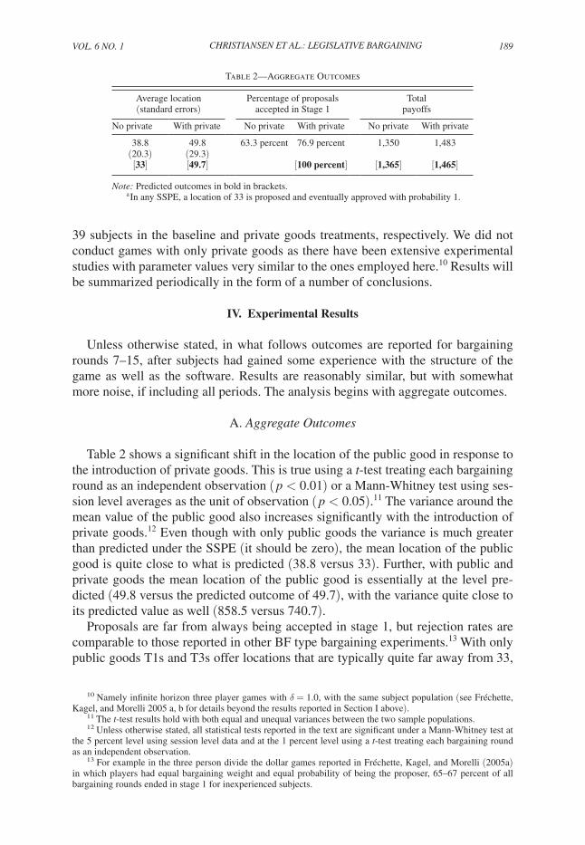
Table 2 shows a significant shift in the location of the public good in response to the introduction of private goods. This is true using a t-test treating each bargaining round as an independent observation ( p < 0.01) or a Mann-Whitney test using ses-sion level averages as the unit of observation ( p < 0.05).11 The variance around the mean value of the public good also increases significantly with the introduction of private goods.12 Even though with only public goods the variance is much greater than predicted under the SSPE (it should be zero), the mean location of the public good is quite close to what is predicted (38.8 versus 33). Further, with public and private goods the mean location of the public good is essentially at the level pre-dicted (49.8 versus the predicted outcome of 49.7), with the variance quite close to its predicted value as well (858.5 versus 740.7).
Proposals are far from always being accepted in stage 1, but rejection rates are comparable to those reported in other BF type bargaining experiments.13 With only public goods T1s and T3s offer locations that are typically quite far away from 33,
10 Namely infinite horizon three player games with δ = 1.0, with the same subject population (see Fréchette, Kagel, and Morelli 2005 a, b for details beyond the results reported in Section I above).
11 The t-test results hold with both equal and unequal variances between the two sample populations.12 Unless otherwise stated, all statistical tests reported in the text are significant under a Mann-Whitney test at
the 5 percent level using session level data and at the 1 percent level using a t-test treating each bargaining round as an independent observation.
13 For example in the three person divide the dollar games reported in Fréchette, Kagel, and Morelli (2005a) in which players had equal bargaining weight and equal probability of being the proposer, 65–67 percent of all bargaining rounds ended in stage 1 for inexperienced subjects.
Table 2—Aggregate Outcomes
Average location(standard errors)
Percentage of proposalsaccepted in Stage 1
Total payoffs
No private With private No private With private No private With private
38.8 49.8 63.3 percent 76.9 percent 1,350 1,483(20.3) (29.3)[33] [49.7] [100 percent] [1,365] [1,465]
Note: Predicted outcomes in bold in brackets.a In any SSPE, a location of 33 is proposed and eventually approved with probability 1.
190 AMEriCAN ECoNoMiC JourNAL: MiCroECoNoMiCs fEBruAry 2014
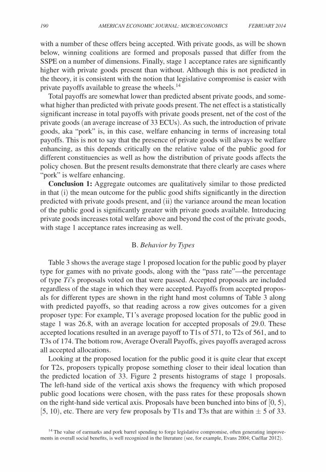
with a number of these offers being accepted. With private goods, as will be shown below, winning coalitions are formed and proposals passed that differ from the SSPE on a number of dimensions. Finally, stage 1 acceptance rates are significantly higher with private goods present than without. Although this is not predicted in the theory, it is consistent with the notion that legislative compromise is easier with private payoffs available to grease the wheels.14
Total payoffs are somewhat lower than predicted absent private goods, and some-what higher than predicted with private goods present. The net effect is a statistically significant increase in total payoffs with private goods present, net of the cost of the private goods (an average increase of 33 ECUs). As such, the introduction of private goods, aka “pork” is, in this case, welfare enhancing in terms of increasing total payoffs. This is not to say that the presence of private goods will always be welfare enhancing, as this depends critically on the relative value of the public good for different constituencies as well as how the distribution of private goods affects the policy chosen. But the present results demonstrate that there clearly are cases where “pork” is welfare enhancing.
Conclusion 1: Aggregate outcomes are qualitatively similar to those predicted in that (i) the mean outcome for the public good shifts significantly in the direction predicted with private goods present, and (ii) the variance around the mean location of the public good is significantly greater with private goods available. Introducing private goods increases total welfare above and beyond the cost of the private goods, with stage 1 acceptance rates increasing as well.
B. Behavior by Types
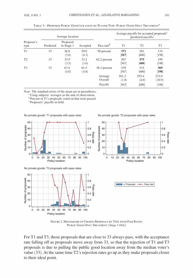
Table 3 shows the average stage 1 proposed location for the public good by player type for games with no private goods, along with the “pass rate”—the percentage of type T i’s proposals voted on that were passed. Accepted proposals are included regardless of the stage in which they were accepted. Payoffs from accepted propos-als for different types are shown in the right hand most columns of Table 3 along with predicted payoffs, so that reading across a row gives outcomes for a given proposer type: For example, T1’s average proposed location for the public good in stage 1 was 26.8, with an average location for accepted proposals of 29.0. These accepted locations resulted in an average payoff to T1s of 571, to T2s of 561, and to T3s of 174. The bottom row, Average Overall Payoffs, gives payoffs averaged across all accepted allocations.
Looking at the proposed location for the public good it is quite clear that except for T2s, proposers typically propose something closer to their ideal location than the predicted location of 33. Figure 2 presents histograms of stage 1 proposals. The left-hand side of the vertical axis shows the frequency with which proposed public good locations were chosen, with the pass rates for these proposals shown on the right-hand side vertical axis. Proposals have been bunched into bins of [0, 5), [5, 10), etc. There are very few proposals by T1s and T3s that are within ± 5 of 33.
14 The value of earmarks and pork barrel spending to forge legislative compromise, often generating improve-ments in overall social benefits, is well recognized in the literature (see, for example, Evans 2004; Cuéllar 2012).
VoL. 6 No. 1 191christiansen et al.: legislative bargaining
For T1 and T3, those proposals that are close to 33 always pass, with the acceptance rate falling off as proposals move away from 33, so that the rejection of T1 and T3 proposals is due to pulling the public good location away from the median voter’s value (33). At the same time T2’s rejection rates go up as they make proposals closer to their ideal point.
Figure 2. Histograms of Chosen Proposals by Type with Pass Rates: Public Good Only Treatment (stage 1 only)
Table 3—Proposed Public Good Location by Player Type: Public Good Only Treatmenta
Average locationAverage payoffs for accepted proposalsc
[predicted payoffs]Proposer’s type Predicted
Proposed in Stage 1 Accepted Pass rateb T1 T2 T3
T1 33 26.8 29.0 50 percent 571 561 174(3.6) (4.3) [567] [600] [198]
T2 33 33.9 33.2 62.2 percent 567 575 199(3.5) (3.6) [567] [600] [198]
T3 33 67.6 61.5 38.3 percent 539 515 369(4.0) (4.8) [567] [600] [198]
Average 561.2 555.4 233.0Overall (1.8) (4.0) (10.9)Payoffs [567] [600] [198]
Note: The standard errors of the mean are in parentheses.a Using subjects’ averages as the unit of observation.b Percent of T i ’s proposals voted on that were passed.c Proposers’ payoffs in bold.
Pass rate
Num
ber
of p
ropo
sals
Policy location
# Proposals Pass rate
No private goods: T1 proposals with pass rates
0
0.2
0.4
0.6
0.8
1
0
0.2
0.4
0.6
0.8
1
Pass rate
0
10
20
30
40
50
0
10
20
30
40
50
Num
ber
of p
ropo
sals
0 10 20 30 40 50 60 70 80 90 1000 10 20 30 40 50 60 70 80 90 100
0
0.2
0.4
0.6
0.8
1
0
10
20
30
40
50
0 10 20 30 40 50 60 70 80 90 100
Policy location
No private goods: T2 proposals with pass rates
Pass rate
Num
ber
of p
ropo
sals
Policy location
No private goods: T3 proposals with pass rates
192 AMEriCAN ECoNoMiC JourNAL: MiCroECoNoMiCs fEBruAry 2014
Contrary to the SSPE, there is at least modest proposer power present for all three types, in that each of them obtains their highest average payoff when propos-ing. In this respect T3s have the strongest proposer power, which is only partially offset by their much lower acceptance rates compared to T1s and T2s.15 To rank relative proposer power we calculate expected payoffs to the different types in their role as proposers and compare it to what is predicted under the SSPE.16 T3s aver-aged 144 percent of what is predicted under the SSPE compared to 100 percent and 95 percent for T1s and T2s, respectively.17 T1s wind up with essentially the same average overall payoffs as T2s as they get a little more than predicted on average as proposers, and T2s have a higher unit cost to the deviations from their ideal point.
Proposals typically passed with what essentially amounted to minimum winning coalitions (MWCs) as winning proposals averaged 1.2 votes (in addition to the pro-poser’s vote), with minimal variation across proposer types. Winning coalitions are what one would expect based on players’ self-interest with T2s most often voting in favor of T1’s proposals (87 percent), T1s typically siding with T2s (74 percent), and T2s typically siding with T3s (65 percent).
The failure of all proposals passed to be within a couple of ECUs from the median voter’s value (33) can potentially be attributed to impatience on the part of subjects. Even though δ = 1, it is possible that T2s are willing to accept something short of their ideal point simply to get the bargaining round over with. However, it is clear that impatience cannot provide a full explanation for the failure to achieve T2’s ideal point. Although an impatient T2 would allow T1 and T3 proposers to pull the policy location closer to their respective ideal points, if T2 voters are impatient we would expect the same to be true of T1s and T3s. As such T2s should be able to consistently propose and pass a policy location of 33. But Figure 2 shows that T2s proposing policies between 30 and 35 get their proposals passed less than 40 percent of the time. Further evidence that impatience cannot provide a full explanation for the failure to achieve T2’s ideal point comes from ultimatum game experiments, where impatience plays no role, yet there are consistent failures to achieve anything approaching the subgame perfect equilibrium outcome. Finally, to the extent that impatience plays a role here, we would expect it to play a comparable role when private goods are available. As such, the comparative static predictions of the model, which is what we are primarily interested in, should be preserved going between games with and without private goods.
Conclusion 2: The relatively large variance around the predicted location of 33 with public goods results from T1s and T3s proposing locations closer to their ideal points with many of these proposals accepted. MWCs tend to form based on voters’ self-interest, with the vast majority of proposals passing with one other vote in addi-tion to the proposer.
15 Fréchette, Kagel, and Morelli (2005c) also identify proposer power where it is not predicted under the SSPE in legislative bargaining games.
16 The expected payoff is a proposer’s average payoff in accepted allocations multiplied by the average accep-tance rate plus their empirically determined continuation value of the game multiplied by the average rejection rate.
17 Note that T2’s predicted payoff (600) is the maximum payoff possible in the game, while T3’s predicted payoff is substantially below this. As a result, T3s have much more room for improving their predicted payoff.
VoL. 6 No. 1 193christiansen et al.: legislative bargaining
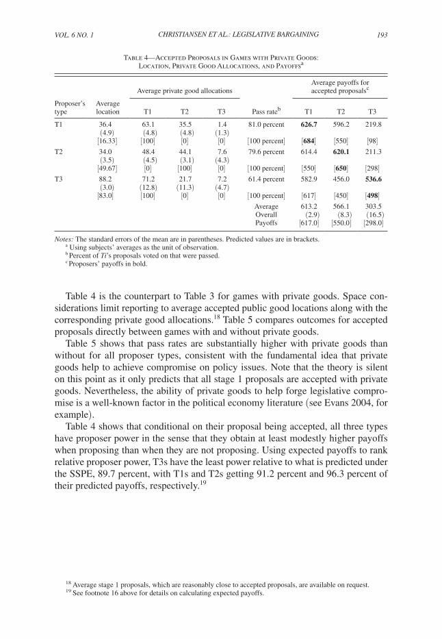
Table 4 is the counterpart to Table 3 for games with private goods. Space con-siderations limit reporting to average accepted public good locations along with the corresponding private good allocations.18 Table 5 compares outcomes for accepted proposals directly between games with and without private goods.
Table 5 shows that pass rates are substantially higher with private goods than without for all proposer types, consistent with the fundamental idea that private goods help to achieve compromise on policy issues. Note that the theory is silent on this point as it only predicts that all stage 1 proposals are accepted with private goods. Nevertheless, the ability of private goods to help forge legislative compro-mise is a well-known factor in the political economy literature (see Evans 2004, for example).
Table 4 shows that conditional on their proposal being accepted, all three types have proposer power in the sense that they obtain at least modestly higher payoffs when proposing than when they are not proposing. Using expected payoffs to rank relative proposer power, T3s have the least power relative to what is predicted under the SSPE, 89.7 percent, with T1s and T2s getting 91.2 percent and 96.3 percent of their predicted payoffs, respectively.19
18 Average stage 1 proposals, which are reasonably close to accepted proposals, are available on request.19 See footnote 16 above for details on calculating expected payoffs.
Table 4—Accepted Proposals in Games with Private Goods: Location, Private Good Allocations, and Payoffsa
Average private good allocationsAverage payoffs for accepted proposalsc
Proposer’s type
Average location T1 T2 T3 Pass rateb T1 T2 T3
T1 36.4 63.1 35.5 1.4 81.0 percent 626.7 596.2 219.8(4.9) (4.8) (4.8) (1.3)
[16.33] [100] [0] [0] [100 percent] [684] [550] [98]T2 34.0 48.4 44.1 7.6 79.6 percent 614.4 620.1 211.3
(3.5) (4.5) (3.1) (4.3)[49.67] [0] [100] [0] [100 percent] [550] [650] [298]
T3 88.2 71.2 21.7 7.2 61.4 percent 582.9 456.0 536.6(3.0) (12.8) (11.3) (4.7)
[83.0] [100] [0] [0] [100 percent] [617] [450] [498]Average 613.2 566.1 303.5Overall (2.9) (8.3) (16.5)Payoffs [617.0] [550.0] [298.0]
Notes: The standard errors of the mean are in parentheses. Predicted values are in brackets.a Using subjects’ averages as the unit of observation.b Percent of Ti’s proposals voted on that were passed.c Proposers’ payoffs in bold.
194 AMEriCAN ECoNoMiC JourNAL: MiCroECoNoMiCs fEBruAry 2014
Table 5—Comparison of Accepted Proposals in Games With and Without Private Goodsa
Proposer’stype
Average location Pass rate
NoPrv Prv NoPrv Prv
Panel AT1 29.0 36.4** 50.0 percent 81.0 percent***T2 33.2 34.0 62.2 percent 79.6 percent**T3 61.5 88.2*** 38.3 percent 61.4 percent**
Average payoffsb
Proposer’stype
T1 T2 T3
NoPrv Prv NoPrv Prv NoPrv Prv
Panel BT1 571 627 561 596 174 220T2 567 614 575 620 199 211T3 539 583 515 456 369 537
a Using subjects’ averages as the unit of observation.b We do not examine the statistical significance of differences in payoffs since the game
with private goods has an additional 100 ECUs available.*** Difference between private and no private outcomes is significantly different from 0 at
better than the 0.01 level using a t-test with unequal variances and treating each accepted pro-posal as a unit of observation.20
** Difference between private and no private outcomes is significantly different from 0 at better than the 0.05 level using a t-test with unequal variances and treating each accepted proposal as a unit of observation.
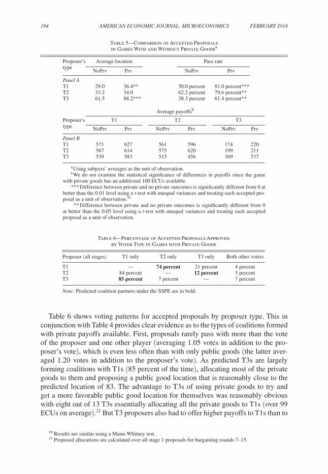
Table 6 shows voting patterns for accepted proposals by proposer type. This in conjunction with Table 4 provides clear evidence as to the types of coalitions formed with private payoffs available. First, proposals rarely pass with more than the vote of the proposer and one other player (averaging 1.05 votes in addition to the pro-poser’s vote), which is even less often than with only public goods (the latter aver-aged 1.20 votes in addition to the proposer’s vote). As predicted T3s are largely forming coalitions with T1s (85 percent of the time), allocating most of the private goods to them and proposing a public good location that is reasonably close to the predicted location of 83. The advantage to T3s of using private goods to try and get a more favorable public good location for themselves was reasonably obvious with eight out of 13 T3s essentially allocating all the private goods to T1s (over 99 ECUs on average).21 But T3 proposers also had to offer higher payoffs to T1s than to
20 Results are similar using a Mann-Whitney test.21 Proposed allocations are calculated over all stage 1 proposals for bargaining rounds 7–15.
Table 6—Percentage of Accepted Proposals Approved by Voter Type in Games with Private Goods
Proposer (all stages) T1 only T2 only T3 only Both other voters
T1 — 74 percent 21 percent 4 percentT2 84 percent — 12 percent 5 percentT3 85 percent 7 percent — 7 percent
Note: Predicted coalition partners under the SSPE are in bold.
VoL. 6 No. 1 195christiansen et al.: legislative bargaining
themselves as predicted by the theory. Of T3 proposals that pass only with the vote of a T1, T3s’ payoffs were 32 ECUs lower on average than T1s’ payoffs. The remainder of the T3s either kept a significant portion of private goods for themselves and/or allocated a significant portion to T2s.22
Contrary to the SSPE prediction, T2s primarily formed coalitions with T1s (84 percent of the time), with only 3 out of 13 proposing an average location greater than 36, compared to 4 proposing average locations less than 30.23 The SSPE predic-tion that T2s will form coalitions with T3s is reasonably subtle as it essentially rests on the fact that T1s can demand relatively large payoffs unless T2s form coalitions with T3s. However, T1s do not demand significantly higher payoffs, with the near equal splits T2s offer T1s being readily accepted. Note that T2s earned very close to what they would have gotten under the SSPE (630 on average for proposals that pass with only T1’s vote versus 650 under the SSPE),24 while also having their proposals accepted with a very high frequency. With so few proposals actually made by T2s to T3s we can only speculate what it would have taken for T2s to form successful coali-tions with T3s. This no doubt would have required a public good location far above 33 to get T3’s vote, which would have reduced T2’s earnings substantially compared to what they got partnering with T1s.25 T1s primarily formed coalitions with T2s (74 percent of the time), with 9 out of 13 T1s’ average stage 1 proposals yielding payoffs that were within plus or minus 20 ECUs of T2s’ payoffs. These proposals involved sharply lower payoffs for T3s (350 ECUs more to T1 than to T3).26
Conclusion 3: All proposers’ acceptance rates are substantially higher with private goods available to “grease the wheels,” consistent with the fundamental notion that private goods help to achieve legislative compromise. Comparing actual to expected payoffs, T2s have the greatest proposer power relative to what the SSPE predicts, followed by T1s and T3s. T3s largely form coalitions with T1s, as predicted. However, T2s form winning coalitions with T1s, contrary to what the SSPE predicts.
C. Behavior by Types
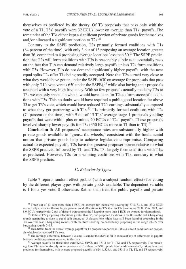
Table 7 reports random effect probits (with a subject random effect) for voting by the different player types with private goods available. The dependent variable is 1 for a yes vote; 0 otherwise. Rather than treat the public payoffs and private
22 Three out of 13 kept more than 1 ECU on average for themselves (averaging 77.8, 33.1, and 23.2 ECUs respectively), with 4 offering larger private good allocations to T2s than to T1s (averaging 77.8, 55.6, 38.3, and 8.9 ECUs respectively; 2 out of these 4 were among the 3 keeping more than 1 ECU on average for themselves).
23 Of those T2s proposing allocations greater than 36, one proposed locations in the 80s in the last 4 bargaining rounds generating a close to equal split among all 3 players, one might have still been learning proposing in the 30s over the last 6 bargaining rounds, with the third showing no consistency proposing in the range 21–85 over bargaining rounds 7–15.
24 This differs from the overall average payoff for T2 proposers reported in Table 4 since it conditions on propos-als which only received T1’s vote.
25 The earnings differential between T2s and T3s under the SSPE is far in excess of any of differences in payoffs between coalition partners reported in the data.
26 Average payoffs for these nine were 626.7, 619.5, and 181.2 for T1, T2, and T3, respectively. The remain-ing four T1s were uniformly more generous to T3s than the SSPE prediction, while consistently taking less than predicted for themselves, with average proposed payoffs of 624.1, 526.4, and 333.8 to T1, T2, and T3 respectively.
196 AMEriCAN ECoNoMiC JourNAL: MiCroECoNoMiCs fEBruAry 2014
payoffs as separate explanatory variables, we adopt a reduced form approach with own payoffs as right-hand side variables distinguishing between who the proposer is (in case there is resentment towards different proposer types on account of unequal payoffs), as well as payoffs of proposers to other players (to account for possible other regarding preferences).27 For example, the first probit reported is for how T1s voted with the following RHS variables: T2’s proposed payoff to T1 when T2’s pro-posal was voted on, T3’s proposed payoff to T1 when T3’s proposal was voted on, T2’s proposed payoff to T3 when T2’s proposal was voted on (T2T3), T3’s proposed payoff to T2 when T3’s proposal was voted on (T3T2), with a dummy variable that takes value 1 when T3 is the proposer, and 0 when T2 is the proposer.28 Preliminary probits with voting stage included as an explanatory variable failed to identify a sig-nificant stage effect ( p > 0.10 in all cases) with little impact on the other coefficient values with stage removed, and are not reported here.
Own payoffs are positive and significantly different from zero at better than the 10 percent level in all cases. The sole exception to this is T3’s voting in response to own payoffs which are not significant at conventional levels. This probably reflects the infrequency with which T1s and T2s offered any sizable share to T3s. T2s are “color” blind when voting with respect to the proposer’s type, as we cannot reject a null hypothesis of equal responsiveness to own share regardless of the proposer’s type, and the DT3 dummy is not significantly different from zero as well. The situation is more complicated for T1 voters who, other things equal are more likely to accept a proposal from a T3 (the DT3 dummy is significant at the 5 percent level), but for whom a two-tailed t-test rejects the null hypothesis that they are equally responsive to changes in own payoffs from T2 and T3 proposers. Instead, they are more responsive to payoffs from T2 proposers. T1 voters also appear to favor
27 We also ran regressions like those reported in Table 7 breaking out payoffs from private and public goods, testing for any differences in coefficient values. In no case could we reject the null hypothesis that the coefficients were equal. While the reduced form is applicable here, the idea that these two are perfect substitutes in field settings may well not be the case. We also ran (subject) fixed effect regressions, and regressions with errors clustered at the subject level, with very similar results.
28 The DT3 dummy is included to account for any potential fixed differential responsiveness T1s might employ in determining whether to vote for or against T1s’ proposals. The DT3 and DT1 dummies in T2 and T3’s voting regressions play the same role there as well.
Table 7—Voting Probits with Private Goods Available (Rounds 7–15)
T1 Vote = −60.3 +0.094 T2 +0.017 T3 +0.020 T2T3 −0.004 T3T2 +52.598 DT3(20.4)*** (0.031)*** (0.010)* (0.009)** (0.006) (21.5)**
T2 Vote = −20.8 +0.036 T1 +0.037 T3 +0.002 T1T3 −0.004 T3T1 +2.999 DT3(8.2)** (0.013)*** (0.023)* (0.004) (0.022) (20.0)
T3 Vote = −0.95 −0.001 T1 +0.012 T2 −0.026 T1T2 −0.006 T2T1 15.102 DT1(16.76) (0.006) (0.010) (0.018) (0.024) (19.3)
Note: Dependent variable is 1 if vote in favor of proposal; 0 otherwise.
Explanatory variables: T i = payoff proposed by player T i to responder in question; T i Tj = payoff proposed by Ti to other player, Tj, as part of the proposal to responder in question; D T i = dummy variable equal to 1 for proposer of type T i, 0 otherwise.*** Significant at the 1 percent level. ** Significant at the 5 percent level. * Significant at the 10 percent level.
VoL. 6 No. 1 197christiansen et al.: legislative bargaining
T2 proposals that target higher payoffs to T3s (the significant positive coefficient value for T2T3). None of the remaining variables in the probits achieve statistical significance at anything approaching conventional levels.
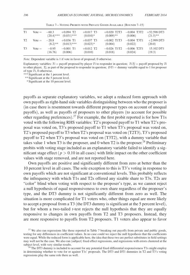
The probits can be used to calculate the expected payoff maximizing proposal for each type, as well as the expected payoff from the SSPE proposal, and the “effi-cient equal split” (the payoff maximizing proposal that equalizes payoffs to within one ECU between the proposer and one other coalition partner). These are reported in Table 8 along with the average expected return by types when proposing.29, 30 Several things stand out in the data. First, the payoff maximizing proposal is greater than the SSPE proposal in all cases. This results from the relatively high rejection rates that the very unequal splits under the SSPE generate. Second, the efficient equal split also yields a higher expected payoff than the SSPE for all types, but a lower expected return than the payoff maximizing proposal (although not so much lower that proposers’ are giving up large sums of money). Third, for T2s both the payoff maximizing proposal and the efficient equal split involve partnering with T1s, not T3s as the SSPE requires, yielding substantially higher payoffs than the SSPE in both cases. Finally, in terms of looking for an efficient equal split it is a relative no-brainer for T3s to partner with T1s rather than T2s as T3s would earn 534
29 The expected payoff of an offer depends on the probability one or both of the other players accept the pro-posal, the proposer’s type, and the experimental continuation value for the game should the proposal be defeated. The latter is a type’s average payoff in the game weighted by the frequency of acceptance for each type of proposer. The experimental continuation values are 613, 566, and 304 for T1, T2, and T3, respectively.
30 In calculating the payoff maximizing proposal for T1s, along with the expected returns from the SSPE pro-posal and the efficient equal split, we restricted the T1T2 coefficient value to zero in the T3 voter regression since (i) the coefficient value is not significantly different from zero and (ii) without this restriction the payoff maximiz-ing proposal has T1s propose y = 0 and PT1 = 100. This occurs because the probability T3 accepts increases as T2’s payoff declines if T1T2 is included, but the proposal yields a payoff to T3s of 0, with 700 for T1s. It is totally implausible that T3s would vote for such proposals, so that extrapolation of the probits in this case is unreasonable. This is empirically supported by the fact that in only 2 out of 41 cases T3s voted in favor of a T1 proposal which gave them a payoff of 200 or less.
Table 8—Comparison of Expected Return to Proposer’s Payoff Maximizing Proposal with Other Offers in Games with Private Goods (standard error of the mean in parentheses)a
Expected return to proposer from
Proposer’s typePayoff maximizing
proposalEfficient
equal splitb SSPEAverage expected
returnc
T1 660.4 633.8 627.3 625.5(2.97)
T2 645.8 633.9 587.4 615.9(6.36)
T3 543.8 543.8 465.4 473.1(16.37)
a Using subjects’ averages as the unit of observation.b The payoff maximizing proposal that equalizes payoffs (within one ECU) between the proposer and one other
coalition partner. The efficient splits are:T1 Proposer: y = 33, PT1 = 67, PT2 = 33, PT3 = 0T2 Proposer: y = 33, PT1 = 66, PT2 = 34, PT3 = 0T3 Proposer: y = 100, PT1 = 100, PT2 = 0, PT3 = 0, where PT i = private goods to T i.c Using subject averages as the unit of observation. Considers all proposals voted on.
198 AMEriCAN ECoNoMiC JourNAL: MiCroECoNoMiCs fEBruAry 2014
under an efficient equal split with T2s versus 600 with T1s, while also providing T1s with a higher payoff thereby promoting greater acceptance rates.31
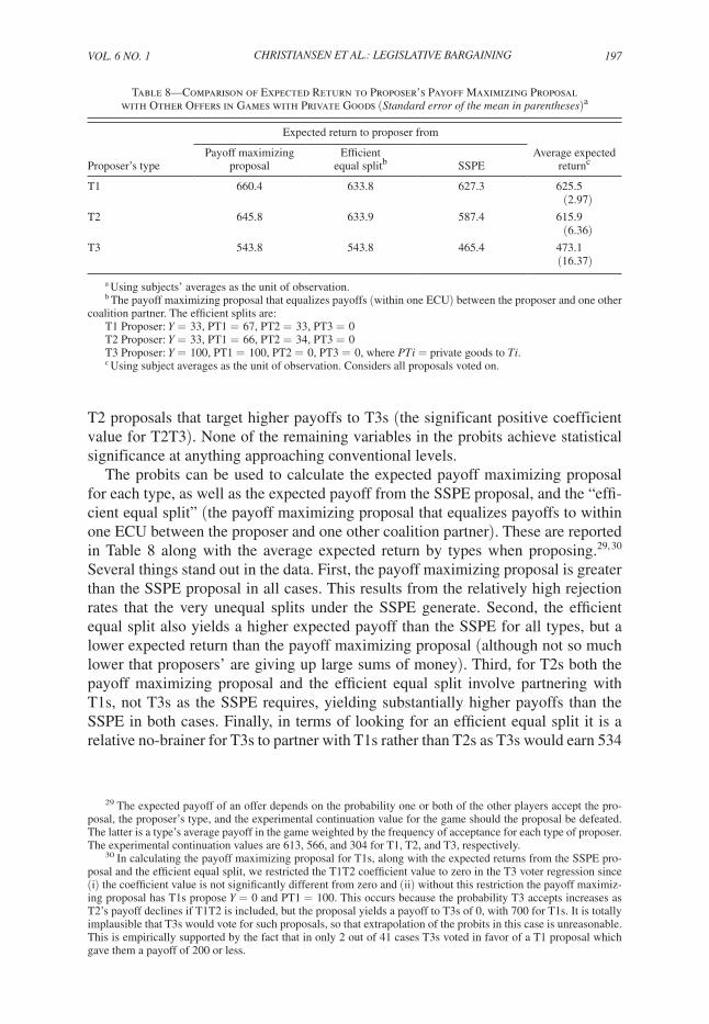
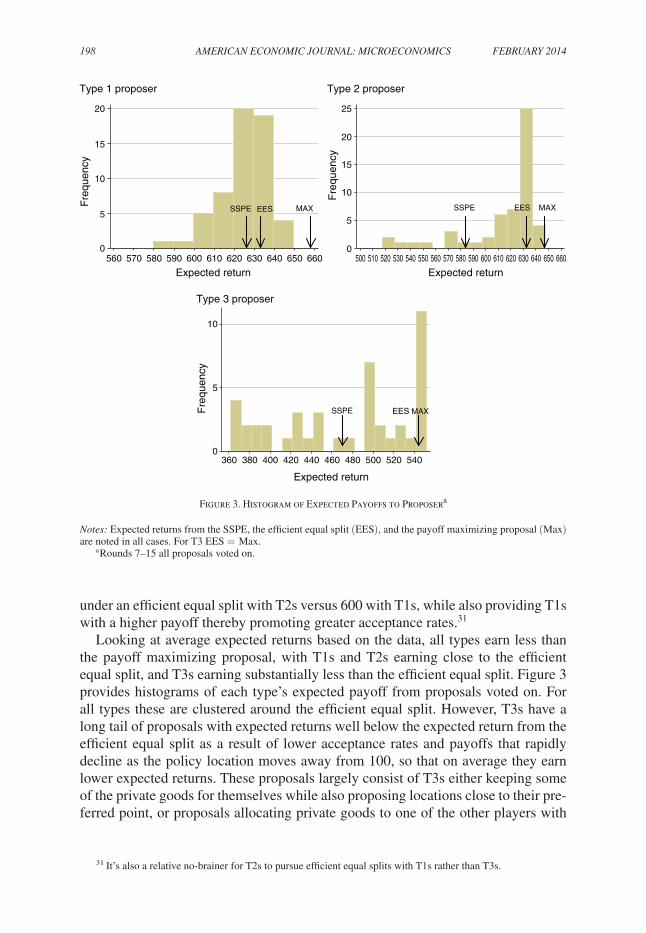
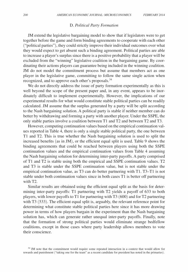
Looking at average expected returns based on the data, all types earn less than the payoff maximizing proposal, with T1s and T2s earning close to the efficient equal split, and T3s earning substantially less than the efficient equal split. Figure 3 provides histograms of each type’s expected payoff from proposals voted on. For all types these are clustered around the efficient equal split. However, T3s have a long tail of proposals with expected returns well below the expected return from the efficient equal split as a result of lower acceptance rates and payoffs that rapidly decline as the policy location moves away from 100, so that on average they earn lower expected returns. These proposals largely consist of T3s either keeping some of the private goods for themselves while also proposing locations close to their pre-ferred point, or proposals allocating private goods to one of the other players with
31 It’s also a relative no-brainer for T2s to pursue efficient equal splits with T1s rather than T3s.
Type 1 proposer Type 2 proposer
Type 3 proposer
0
5
10
15
20
Fre
quen
cy
560 570 580 590 600 610 620 630 640 650 660
Expected return
0
5
10
15
20
25
Fre
quen
cy
500 510 520 530 540 550 560 570 580 590 600 610 620 630 640 650 660
Expected return
0
5
10
Fre
quen
cy
360 380 400 420 440 460 480 500 520 540
Expected return
MAXEES SSPE MAXEES SSPE
SSPE EES MAX
Figure 3. Histogram of Expected Payoffs to Proposera
Notes: Expected returns from the SSPE, the efficient equal split (EES), and the payoff maximizing proposal (Max) are noted in all cases. For T3 EES = Max.
a Rounds 7–15 all proposals voted on.
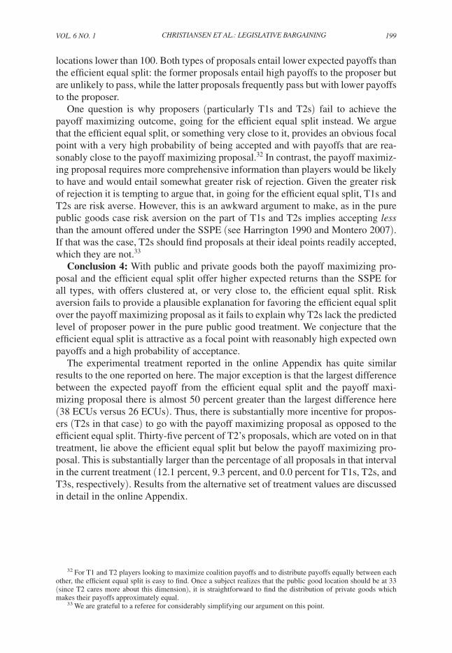
VoL. 6 No. 1 199christiansen et al.: legislative bargaining
locations lower than 100. Both types of proposals entail lower expected payoffs than the efficient equal split: the former proposals entail high payoffs to the proposer but are unlikely to pass, while the latter proposals frequently pass but with lower payoffs to the proposer.
One question is why proposers (particularly T1s and T2s) fail to achieve the payoff maximizing outcome, going for the efficient equal split instead. We argue that the efficient equal split, or something very close to it, provides an obvious focal point with a very high probability of being accepted and with payoffs that are rea-sonably close to the payoff maximizing proposal.32 In contrast, the payoff maximiz-ing proposal requires more comprehensive information than players would be likely to have and would entail somewhat greater risk of rejection. Given the greater risk of rejection it is tempting to argue that, in going for the efficient equal split, T1s and T2s are risk averse. However, this is an awkward argument to make, as in the pure public goods case risk aversion on the part of T1s and T2s implies accepting less than the amount offered under the SSPE (see Harrington 1990 and Montero 2007). If that was the case, T2s should find proposals at their ideal points readily accepted, which they are not.33
Conclusion 4: With public and private goods both the payoff maximizing pro-posal and the efficient equal split offer higher expected returns than the SSPE for all types, with offers clustered at, or very close to, the efficient equal split. Risk aversion fails to provide a plausible explanation for favoring the efficient equal split over the payoff maximizing proposal as it fails to explain why T2s lack the predicted level of proposer power in the pure public good treatment. We conjecture that the efficient equal split is attractive as a focal point with reasonably high expected own payoffs and a high probability of acceptance.
The experimental treatment reported in the online Appendix has quite similar results to the one reported on here. The major exception is that the largest difference between the expected payoff from the efficient equal split and the payoff maxi-mizing proposal there is almost 50 percent greater than the largest difference here (38 ECUs versus 26 ECUs). Thus, there is substantially more incentive for propos-ers (T2s in that case) to go with the payoff maximizing proposal as opposed to the efficient equal split. Thirty-five percent of T2’s proposals, which are voted on in that treatment, lie above the efficient equal split but below the payoff maximizing pro-posal. This is substantially larger than the percentage of all proposals in that interval in the current treatment (12.1 percent, 9.3 percent, and 0.0 percent for T1s, T2s, and T3s, respectively). Results from the alternative set of treatment values are discussed in detail in the online Appendix.
32 For T1 and T2 players looking to maximize coalition payoffs and to distribute payoffs equally between each other, the efficient equal split is easy to find. Once a subject realizes that the public good location should be at 33 (since T2 cares more about this dimension), it is straightforward to find the distribution of private goods which makes their payoffs approximately equal.
33 We are grateful to a referee for considerably simplifying our argument on this point.
200 AMEriCAN ECoNoMiC JourNAL: MiCroECoNoMiCs fEBruAry 2014
D. Political Party formation
JM extend the legislative bargaining model to show that if legislators were to get together before the game and form binding agreements to cooperate with each other (“political parties”), they could strictly improve their individual outcomes over what they would expect to get absent such a binding agreement. Political parties are able to increase a player’s surplus since there is a positive probability that a player will be excluded from the “winning” legislative coalition in the bargaining game. By coor-dinating their actions players can guarantee being included in the winning coalition. JM do not model the commitment process but assume that members act as one player in the legislative game, committing to follow the same single action when recognized, and to approve each other’s proposals.34
We do not directly address the issue of party formation experimentally as this is well beyond the scope of the present paper and, in any event, appears to be inor-dinately difficult to implement experimentally. However, the implications of our experimental results for what would constitute stable political parties can be readily calculated. JM assume that the surplus generated by a party will be split according to the Nash bargaining solution. A political party is stable if neither member can do better by withdrawing and forming a party with another player. Under the SSPE, the only stable parties involve a coalition between T1 and T2 and between T2 and T3.
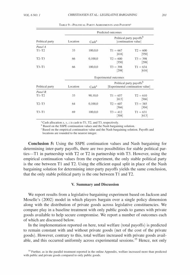
However, computing continuation values based on the empirical continuation val-ues reported in Table 4, there is only a single stable political party, the one between T1 and T2. This is true whether the Nash bargaining solution is used to split the increased benefits (as in JM), or the efficient equal split is used. Table 9 shows the binding agreements that could be reached between players using both the SSPE continuation values and the empirical continuation values from Table 4 assuming the Nash bargaining solution for determining inter-party payoffs. A party comprised of T1 and T2 is stable using both the empirical and SSPE continuation values. T2 and T3 is stable under the SSPE continuation value, but is not stable under the empirical continuation value, as T3 can do better partnering with T1. T3–T1 is not stable under both continuation values since in both cases T1 is better off partnering with T2.
Similar results are obtained using the efficient equal split as the basis for deter-mining inter-party payoffs: T1 partnering with T2 yields a payoff of 633 to both players, with lower payoffs to T1 for partnering with T3 (600) and for T2 partnering with T3 (533). The efficient equal split is, arguably, the relevant reference point for determining what constitute stable political parties here since it has more drawing power in terms of how players bargain in the experiment than the Nash bargaining solution has, which can generate rather unequal inter-party payoffs. Finally, note that the formation of strong political parties would eliminate strange bedfellow coalitions, except in those cases where party leadership allows members to vote their conscience.
34 JM note that the commitment would require some repeated interaction in a context that would allow for rewards and punishment (“taking one for the team” as a recent candidate for president has noted in the primaries).
VoL. 6 No. 1 201christiansen et al.: legislative bargaining
Conclusion 5: Using the SSPE continuation values and Nash bargaining for determining inter-party payoffs, there are two possibilities for stable political par-ties—T1 in partnership with T2 or T2 in partnership with T3. However, using the empirical continuation values from the experiment, the only stable political party is the one between T1 and T2. Using the efficient equal split in place of the Nash bargaining solution for determining inter-party payoffs yields the same conclusion, that the only stable political party is the one between T1 and T2.
V. Summary and Discussion
We report results from a legislative bargaining experiment based on Jackson and Moselle’s (2002) model in which players bargain over a single policy dimension along with the distribution of private goods across legislative constituencies. We compare play in a baseline treatment with only public goods to games with private goods available to help secure compromise. We report a number of outcomes each of which are discussed below.
In the implementation reported on here, total welfare (total payoffs) is predicted to remain constant with and without private goods (net of the cost of the private goods). However, contrary to this, total welfare increased with private goods avail-able, and this occurred uniformly across experimental sessions.35 Hence, not only
35 Further, as in the parallel treatment reported in the online Appendix, welfare increased more than predicted with public and private goods compared to only public goods.
Table 9—Political Party Agreements and Payoffsa
Predicted outcomes
Political party payoffsb
Political party Location Casha [continuation value]
Panel AT1–T2 33 100,0,0 T1 = 667 T2 = 600
[616] [550]T2–T3 66 0,100,0 T2 = 600 T3 = 398
[550] [298]T3–T1 66 100,0,0 T3 = 398 T1 = 634
[298] [616]
Experimental outcomes
Political party payoffsb
Political party Location Casha [Experimental continuation value]
Panel BT1–T2 33 90,10,0 T1 = 657 T2 = 610
[613] [566]T2–T3 64 0,100,0 T2 = 607 T3 = 385
[566] [304]T3–T1 69 100,0,0 T3 = 412 T1 = 631
[304] [613]
a Cash allocation x, y, z is cash to T1, T2, and T3, respectively.b Based on the SSPE continuation values and the Nash bargaining solution.c Based on the empirical continuation value and the Nash bargaining solution. Payoffs and locations are rounded to the nearest integer.
202 AMEriCAN ECoNoMiC JourNAL: MiCroECoNoMiCs fEBruAry 2014
did private goods grease the wheels in terms of securing more timely passage of proposed allocations, they also improved total welfare. This is not to say this will always happen, but that private goods need not always be bad. Additional reser-vations need to be added to this result in efforts to extend it beyond the lab. In the experiment private goods are delivered directly to agents, whereas in field set-tings private goods allocated to legislative districts can take the form of inefficient local public goods; e.g., the “bridge to nowhere” in Alaska. This tends to dilute the benefits obtained from the private good, thereby offsetting, to some extent at least, whatever welfare gains that might result from private goods.36
Regarding total welfare levels reported versus those predicted, total payoffs were less than predicted in the public good only treatment and greater than predicted with private goods. The reason for these deviations can be found in the asymmetric payoffs for deviations from the average public good location in conjunction with the variability in outcomes across different bargaining rounds. The welfare maxi-mizing outcome for the location of the public good is 100, so it always increases total welfare to move policy to the right of the predicted outcome. However, given the costs to deviating, all rightward movements of policy are not equal. The mar-ginal benefit of a rightward shift when the public good location is less than 33 is 4 times the marginal benefit than when its greater than 33 (8 versus 2) as the shift helps both the T2 and T3 players in the first case and helps only the T3 play in the second case. This explains why welfare falls in the public good only treatment even though the average public good location is to the right of 33 (38.8): 53 percent of accepted proposals lie below 33 with an average location of 23.8, while 40 percent of proposals lie above 33 with an average of location of 60.5. That is, given these asymmetric welfare effects around 33, policies passed to the right of 33 do not occur often enough and/or are not sufficiently to the right of 33 for welfare to reach the predicted level.
This asymmetry in welfare effects for deviations from the predicted public good location also explains why welfare is greater than predicted in the private good treat-ment, even though the average accepted policy outcome is almost identical to the average predicted policy. With private goods the average location for the public good with T1s as proposers is 36.4 (with minimal variance around this outcome) versus the predicted location of 16.33, with this difference generating a strong posi-tive welfare effect. So while T2’s average policy location is 34 versus the predicted location of 49.67, it does not usually go below 33 (and when it does, it does not drop below 33 by very much), so that given the asymmetry in payoffs this has a smaller negative impact on total payoffs than the positive effect of the rightward shift in location generated by T1s. Finally, T3 proposers’ average accepted policy location is a bit above the predicted level (88.2 versus 83), which also provides a modest bump to overall welfare.
The public good only treatment achieved, on average, close to the predicted pub-lic good location but with a relatively large variance around that location as opposed to the zero variance predicted. This large variance was generated by T1s and T3s
36 We are grateful to Guillaume Fréchette for pointing this out.
VoL. 6 No. 1 203christiansen et al.: legislative bargaining
consistently proposing a public good location more favorable to their own payoffs than to the median voter (T2), with substantial numbers of these proposals being accepted. Further, as already noted, acceptances were not due to odd coalitions in which T3s voted in favor of T1s’ proposals that favor T1s, and vice versa. Two points are worth discussing with respect to this result. First, there is a series of earlier experiments dealing with public good/locational issues similar to the present study but done in a very different context and with quite different outcomes. These earlier studies typically involved unstructured, face-to-face bargaining using Robert’s rules of order, designed to investigate the drawing power of the core (see Palfrey forth-coming for a survey of the relevant research). A fair summary of these results is that the core represents a fairly good predictor under a number of conditions, but when the core is present and differs from the “fair” outcome where all players receive decent positive payoffs, the fair outcome attracts more attention than the core (Eavey and Miller 1984). Although we find “fair” outcomes within what are effectively MWCs (e.g., much more equal splits between T1s and T2s than predicted) there is typically little concern for the third player, with T3s achieving distinctly lower average payoffs than T1s and T2s in the public good treatment. The factors most likely responsible for this difference from the earlier research are (i) the much more structured nature of the bargaining process under the Baron and Ferejohn (1989) rules employed here which tends to promote MWCs and (ii) the fact that bargain-ing is done anonymously here which tends to promote more unequal splits (see, for example, Roth 1995).37
Predictions of the model regarding potential political party formations are explored as well. Under the SSPE there is the possibility for two stable political parties, one with T1 and T2 as coalition partners and one with T2 and T3 forming a political party. However, based on the experimental outcomes there is only scope for a single stable political party, the one between T1 and T2.
One can always question the relevance of laboratory experiments for behavior outside the lab, particularly in those cases in which payoffs are substantially more equal than the theoretical predictions. However, it can be argued that roughly equal splits will often have considerable drawing power outside the lab where bargain-ers must answer to their constituencies. Equal, or roughly equal splits, are easy to explain to constituents and have considerable saliency of their own. Further, in democratic governments they may have particular power as a challenger in the next election campaign can use substantial differences in outcomes between presumably like type constituencies against the incumbent.
REFERENCES
Baron, David P., and John A. Ferejohn. 1989. “Bargaining in Legislatures.” American Political science review 83 (4): 1181–1206.
Battaglini, Marco, Salvatore Nunnari, and Thomas R. Palfrey. 2012. “Legislative Bargaining and the Dynamics of Public Investment.” American Political science review 106 (4): 407–29.
37 MWCs emerge immediately and grow rapidly in divide the dollar versions of the legislative bargaining game under Baron and Ferejohn (1989) rules, which completely shut out one or more players from positive payoffs (see, for example, Fréchette, Kagel, and Morelli 2005a, b).
204 AMEriCAN ECoNoMiC JourNAL: MiCroECoNoMiCs fEBruAry 2014
Battaglini, Marco, and Thomas R. Palfrey. 2012. “The dynamics of redistributive politics.” Economic Theory 49 (3): 739–77.
Christiansen, Nels. 2010. “Greasing the Wheels: Pork and Public Good Contributions in a Legislative Bargaining Experiment.” http://www.trinity.edu/nchristi/doc/greasing_the_wheels.pdf.
Christiansen, Nels, Sotiris Georganas, and John H. Kagel. 2014. “Coalition Formation in a Legislative Voting Game: Dataset.” American Economic Journal: Microeconomics. http://dx.doi.org/10.1257/mic.6.1.182.
Cuéllar, Mariano-Florentino. 2012. “Earmarking Earmarking.” Stanford Public Law Working Paper 1981836.
Diermeier, Daniel, and Sean Gailmard. 2006. “Self-Interest, Inequality, and Entitlement in Majoritar-ian Decision-Making.” Quarterly Journal of Political science 1 (4): 327–50.
Diermeier, Daniel, and Rebecca Morton. 2005. “Experiments in Majoritarian Bargaining.” In social Choice and strategic Behavior: Essays in the Honor of Jeffrey s. Banks, edited by David Austen-Smith and John Duggan, 201–26. Berlin: Springer-Verlag.
Eavey, Cheryl L., and Gary J. Miller. 1984. “Fairness in Majority Rule Games with a Core.” American Journal of Political science 28 (3): 570–86.
Evans, Diana. 2004. Greasing the Wheels: using Pork Barrel Projects to Build Majority Coalitions in Congress. Cambridge, UK: Cambridge University Press.
Fischbacher, Urs. 2007. “z-Tree: Zurich toolbox for ready-made economic experiments.” Experimen-tal Economics 10 (2): 171–78.
Fréchette, Guillaume R. 2009. “Learning in a multilateral bargaining experiment.” Journal of Econo-metrics 153 (2): 183–95.
Fréchette, Guillaume, John H. Kagel, and Steven F. Lehrer. 2003. “Bargaining in Legislatures: An Experimental Investigation of Open versus Closed Amendment Rules.” American Political science review 97 (2): 221–32.
Fréchette, Guillaume, John H. Kagel, and Massimo Morelli. 2005a. “Nominal bargaining power, selection protocol, and discounting in legislative bargaining.” Journal of Public Economics 89 (8): 1497–1517.
Fréchette, Guillaume, John H. Kagel, and Massimo Morelli. 2005b. “Gamson’s Law versus non-coop-erative bargaining theory.” Games and Economic Behavior 51 (2): 365–90.
Fréchette, Guillaume, John H. Kagel, and Massimo Morelli. 2005c. “Behavioral Identification in Coalitional Bargaining: An Experimental Analysis of Demand Bargaining and Alternating Offers.” Econometrica 73 (6): 1893–1938.
Fréchette, Guillaume, John H. Kagel, and Massimo Morelli. 2012. “Pork versus public goods: an experimental study of public good provision within a legislative bargaining framework.” Economic Theory 49 (3): 779–800.
Harrington, Joseph E., Jr. 1990. “The role of risk preferences in bargaining when acceptance of a pro-posal requires less than unanimous approval.” Journal of risk and uncertainty 3 (2): 135–54.
Jackson, Matthew O., and Boaz Moselle. 2002. “Coalition and Party Formation in a Legislative Voting Game.” Journal of Economic Theory 103 (1): 49–87.
Kagel, John H., Hankyoung Sung, and Eyal Winter. 2010. “Veto power in committees: an experimental study.” Experimental Economics 13 (2): 167–88.
McKelvey, Richard D. 1991. “An Experimental Test of a Stochastic Game Model of Committee Bar-gaining.” In Contemporary Laboratory research in Political Economy, edited by Thomas R. Pal-frey, 139–68. Ann Arbor: University of Michigan Press.
Montero, Maria. 2007. “Inequity Aversion May Increase Inequity.” Economic Journal 117 (519): C192–204.
Palfrey, Thomas R. Forthcoming. “Experiments in Political Economy. ” In The Handbook of Experi-mental Economics, Vol. 2, edited by John H. Kagel and Alvin E Roth. Princeton: Princeton Uni-versity Press.
Roth, Alvin E. 1995. “Bargaining Experiments.” In Handbook of Experimental Economics, Vol. 1, edited by John H. Kagel and Alvin E. Roth, 253–348. Princeton: Princeton University Press.
Volden, Craig, and Alan E. Wiseman. 2007. “Bargaining in Legislatures over Particularistic and Col-lective Goods.” American Political science review 101 (1): 79–92.