Embed Size (px)
Citation preview

1
Coarse Matching
By R. Preston McAfee1
Keywords: Priority pricing, matching, hazard rate, blackout, rolling blackout.

2
California recently used “rolling blackouts” as a means of rationing electricity. In this
arrangement, a few high priority customers such as hospitals are excluded from rationing, but
otherwise customers experience short-lived blackouts without regard to the social or private
importance of their electricity use. Are rolling blackouts that affect virtually every user a good
strategy? Is there a simple way to improve on the random blackout?
Oren, Smith and Wilson (1985) and Wilson (1989) consider means of mitigating the
social consequences of rationing by matching the high value users to the power provision.
Essentially, the goal is to use ex ante pricing, or priority pricing, to insure that high value users
have a higher probability of receiving the good. In these papers, which differ by whether the
pricing is monopolistic or competitive, demand is characterized by a distribution F of values, and
a distribution H of total units available. If a customer with value x obtains a probability of
service y, the total surplus generated is xy.
The first best solution to the allocation problem involves spot markets, which permit the
rationing of the available supply to the highest value customers. Spot markets, however, are not
always feasible – it may be difficult or impossible to contact customers after the realization of
supply, especially when supply disruptions are abrupt. It is possible to implement the spot
market solution using priority pricing. Priority pricing orders customers from highest to lowest
based on customer payments for service reliability, and provides the good in that order – e.g. if
five units are available, the top five in the priority queue obtain the good. With a continuous
distribution of availability, full priority pricing requires a continuum of positions in the queue
and associated priority prices.
The use of a continuum of priorities is not feasible in many circumstances – using many
priorities makes the scheme unwieldy to administer and opaque to consumers. Moreover, if the

3
priority prices are determined by bidding, as is natural, the auction process will be complex and
expensive to operate when there are many service classes. Instead, it is desirable to use a limited
number of priority classes, perhaps just two. The two-class scheme involves two priorities, high
and low. When capacity is insufficient to supply all the high priority customers, capacity is
randomly allocated among high priority customers. When capacity is insufficient to serve all
customers, but more than sufficient to serve the high priority customers, all high priority
customers are served, with the balance randomly allocated among low priority customers. High
priority customers pay a common priority price for their privileged position. How well does
such a scheme perform? The mathematical fact proved in this paper is that if the distributions
satisfy standard hazard rate hypotheses, the social value of using two priorities is at least half of
the gains of using infinitely many priority classes. Thus, the social cost of using simplified
priority pricing schemes may be modest, and outweighed by the benefits of simplicity and
transparency.
Smith’s 1995 marriage model2 provides a convenient illustration of the theory. In this
model, the value of a match is the product of the types of the agents, who can be taken to be men
and women. Suppose that the types are random variables X and Y, and that these are uniformly
distributed on [0,1]. Consider various methods for matching men and women. Using a purely
random assignment of men to women, the average match has a value of ¼½½0 =×=u : the
average value of X is matched to the average value of Y. Perfect matching maximizes the
average value of a match by associating identical values of X and Y, for an average value of
.311
0
2 == ∫∞ dxxu
4
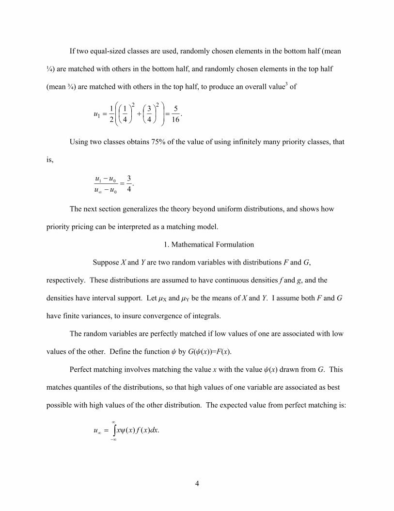
If two equal-sized classes are used, randomly chosen elements in the bottom half (mean
¼) are matched with others in the bottom half, and randomly chosen elements in the top half
(mean ¾) are matched with others in the top half, to produce an overall value3 of
.165
43
41
21 22
1 =
+
=u
Using two classes obtains 75% of the value of using infinitely many priority classes, that
is,
.43
0
01 =−−
∞ uuuu
The next section generalizes the theory beyond uniform distributions, and shows how
priority pricing can be interpreted as a matching model.
1. Mathematical Formulation
Suppose X and Y are two random variables with distributions F and G,
respectively. These distributions are assumed to have continuous densities f and g, and the
densities have interval support. Let mX and mY be the means of X and Y. I assume both F and G
have finite variances, to insure convergence of integrals.
The random variables are perfectly matched if low values of one are associated with low
values of the other. Define the function y by G(y(x))=F(x).
Perfect matching involves matching the value x with the value y(x) drawn from G. This
matches quantiles of the distributions, so that high values of one variable are associated as best
possible with high values of the other distribution. The expected value from perfect matching is:
∫∞
∞−∞ ψ= .)()( dxxfxxu

5
Random matching associates each draw from one distribution with a random draw from
the other, and thus has the overall value u0=mXmY.
Matching with two priority classes and a cutoff point of x* means associating X values
below x* with Y values below y(x*). The function y was chosen so that these have the same
frequency, that is, F(x*)=G(y(x*)) In this case, the social value of matching is:
dyxG
ygydxxF
xfxxFdyxGygydx
xFxfxxFu
xx
xx
∫∫∫∫∞
ψ
∞ψ
∞−∞−ψ−−
−+ψ
=*)(*
*)(*
1 *))((1)(
*)(1)(*))(1(
*))(()(
*)()(*)(
The value u1 arises because low X values, below x*, are associated with low Y values. Thus, the
average match value is the probability of low values F(x*) times the expected value of the low
value match, which is the product of the expected values conditional on being low, plus the
similar term conditional on both being high. This association is perfect in the sense that no low
X values are ever associated with high Y values, but imperfect in the sense of using only two
priority classes.
Priority Pricing: Consider the electricity example of Wilson (1989). Some work is
required to map this example into the framework. There is a distribution of values for the good
or service denoted F, so that 1-F(v) of the population have value for the good exceeding v. 4
There is a distribution of available power H. The natural distributions are in conflicting units –
one in values, one in power – and to streamline the analysis, it is helpful to convert the quantity
units of electricity supply into population service quantiles, that is, into a distribution of service
probabilities. 5 Under priority pricing, a customer with value v is served if there is enough power
to serve all the customers with value at least v, which requires a quantity q ≥ N(1-F(v)), where N
is the total number of customers. The probability the customer of value v is served is the

6
probability that q ≥ N(1-F(v)), which is 1-H(N(1-F(v))).6 In the electricity example, this is the
function y, that is, y(v)= 1-H(N(1-F(v))).
The distribution of service probabilities under priority pricing, then, is the function G
solving G(y(v))=F(v), or G(1-H(N(1-y)))=y. Note that G does not depend on F: G is the feasible
distribution of service priorities and its units are quantiles, not values. If each customer is served
with a probability independent of the customer’s value, the probability that a customer is served
is q/N when there is a supply of q, so that the overall probability of being served is:
dyyNHdyyNHNdyyNhydqqhNqN
∫∫∫∫ −−=−−=−−=1
0
1
0
1
00
))1((1))1((1))1(()1()(
.)()()()()))(1((1000
dyygydvvfvdvvfvFNH ∫∫∫∞∞∞
=ψ=−−=
That is, when the priority assignments are not used, the probability of service is just the
average of the probabilities of service, weighted by the frequency of types. Such a proposition is
true with priority classes as well. For example, suppose that customers with values exceeding v*
are given priority over those with values below v*. Priority means no customer with value below
v* is served when a customer with value above is unserved. In this case, the probability of being
served for a customer with value exceeding v* is
∫∫−
−
×+−
N
vFN
vFN
dqqhdqqhvFN
q
*))(1(
*))(1(
0
)(1)(*))(1(
*)))(1((1*))(1(
)(*)))(1((*))(1(
0
vFNHdqvFN
qHvFNHvFN
−−+−
−−= ∫−
dvvFN
vNfvFNHdqvFNqH
v
vFN
*))(1()()))(1((1
*))(1()(1
*
*))(1(
0 −−−=
−−
= ∫∫∞−

7
dyvG
ygydvvF
vfvvv *))((1
)(*)(1
)()(*)(* ψ−
=−
ψ= ∫∫∞
ψ
∞
Thus, the average probability of service in the high group is just the average of the
probabilities of service of the high group under priority pricing.
The above analysis demonstrates a connection between the priority pricing problem and
the matching problem. From the primitive H, the distribution of power supply, there is a
distribution of service probabilities G, which can be matched to customers in exactly the same
way that the marriage model matches the types of men and women. The distribution G of
service probabilities satisfies G(1-H(N(1-y)))=y.
2. Theorem and Proof
The theorem will require that two commonly used hazard rate conditions apply to
both distributions. These are:
(1) )()(
xfxF and
)()(
ygyG are both increasing, and
(2) )(
)(1xf
xF− and )(
)(1yg
yG− are decreasing.
These conditions are frequently encountered in adverse selection problems, and
they insure that the density does not locally vary too much. When F corresponds to the
distribution of failure times, (2) is equivalent to the requirement that the likelihood of failure
conditioned on no failure having arisen is an increasing function. For example, the probability of
a light bulb failing in the next minute, given that it hasn’t yet failed, grows as the light bulb
ages.7
Theorem: If (1) and (2) hold, and x*=mX, or y(x*)=mY, then .21
0
01 ≥−−
∞ uuuu

8
Proof: The structure of the proof is simple, although the proof is quite long. The
basic structure is to rewrite u•, apply the Cauchy-Schwarz inequality, then recombine so that the
theorem is obvious. The proof starts with a change of variables that dramatically simplifies the
analysis, utilizing the inverses of the distribution functions. Note that )(1 zzF′− is increasing for
z in [0,1] if and only if )()())(()( 1
xfxFxFFxF =
′− is increasing for x in the support of f, and
similarly )()1( 1 zFz′
− − is decreasing if and only if )(
)(1))(())(1( 1
xfxFxFFxF −
=′
− − is
decreasing. Thus, (1) and (2) become:
(3) )(1 zzF′− and )(1 zzG
′− are increasing for z in [0,1], and
(4) )()1( 1 zFz′
− − and )()1( 1 zGz′
− − are decreasing for z in [0,1].
Using the change of variables z=F(x) or z=G(y), note that:
∫∫∫ −−∞
∞−
−∞
∞−∞ ==ψ=
1
0
111 .)()()())(()()( dzzGzFdxxfxFxGdxxfxxu
YXdzzGdzzFdyyygdxxxfu µµ=== ∫∫∫∫ −−∞
∞−
∞
∞−
1
0
11
0
10 )()()()(
and
dyxG
ygydxxF
xfxxFdyxGygydx
xFxfxxFu
xx
xx
∫∫∫∫∞
ψ
∞ψ
∞−∞− ψ−−−+
ψ=
*)(*
*)(*
1 *))((1)(
*)(1)(*))(1(
*))(()(
*)()(*)(
∫∫∫∫ −−−+= −−−−
11
11
0
1
0
11
)(1
)()1()()(cc
cc
cdzzG
cdzzFc
cdzzG
cdzzFc

9
,)()(1
1)()(1 11
11
0
1
0
1 ∫∫∫∫ −−−−
−+=
cc
ccdzzGdzzF
cdzzGdzzF
c
where c=F(x*)=G(y(x*)).
Moreover, it is immediate that
.))(())((1
1))(())((1 1
c
11
c
1c
0
1c
0
101 ∫∫∫∫ µ−µ−
−+µ−µ−=− −−−− dzzGdzzF
cdzzGdzzF
cuu YXYX
The key step in the analysis below involves the inequality
(5) ∫∫∫ µ−×′
≥µ−′ −−−−
c
0
1c
0
1c
0
11 ))(()())()((cdzzF
cdzzzG
cdzzFzzG XX ,
which follows from the fact that )(1 zzG′− and XzF µ−− )(1 are both increasing functions
of z, and hence positively correlated, and thus the expected value of the product exceeds the
product of the expected values.8 This inequality is used in three other guises below, but the logic
is the same. A second fact, used repeatedly, is
∫ −=µ1
0
1 )( dzzFX and .)(1
0
1∫ −=µ dzzGY
Rewrite u• to obtain:
∫∫∫∫ µ−µ−=−=− −−−−−−∞
1
0
111
0
11
0
11
0
110 ))()()(()()()()( dzzGzFdzzGdzzFdzzGzFuu YX
∫∫ µ−µ−+µ−µ−= −−−−1
11c
0
11 ))()()(())()()((c
YXYX dzzGzFdzzGzF
(Integrate by parts to obtain:)

10
∫∫ µ−′
−µ−′
−µ−µ−= −−−−−−c
0
11c
0
1111 ))()(())()(())()()(( dzzFzzGdzzGzzFcGcFc XYYX
∫ µ−′
−+µ−µ−−+ −−−−1
1111 ))()(()1())()()()(1(c
YYX dzzGzFzcGcFc
∫ µ−′
−+ −−1
11 ))()(()1(c
X dzzFzGz
(Collect terms and multiply and divide by c or 1-c)
∫∫ µ−′
−µ−′
−µ−µ−= −−−−−−c
0
11c
0
1111 ))()(())()(())()()((cdzzFzzGc
cdzzGzzFccGcF XYYX
∫∫ −µ−
′−−+
−µ−
′−−+ −−−−
111
111
1))()(()1()1(
1))()(()1()1(
cX
cY c
dzzFzGzcc
dzzGzFzc
(Employ four versions of (5))
∫∫ µ−×′
−µ−µ−≤ −−−−c
0
1c
0
111 ))(()())()()((cdzzG
cdzzzFccGcF YYX
∫∫ µ−×′
− −−c
0
1c
0
1 ))(()(cdzzF
cdzzzGc X
∫∫ −µ−×
−′
−−+ −−1
11
1
1))((
1)()1()1(
cY
c cdzzG
cdzzFzc
∫∫ −µ−×
−′
−−+ −−1
11
1
1))((
1)()1()1(
cX
c cdzzF
cdzzGzc
(Integrate by parts and collect terms)

11
∫ µ−µ−−µ−µ−= −−−−c
0
1111 ))(())(())()()(( dzzGcFcGcF YXYX
∫∫ µ−×µ−+ −−c
0
1c
0
1 ))(())((1 dzzGdzzFc YX
∫∫∫ µ−×µ−+µ−µ−− −−−−c
0
1c
0
1c
0
11 ))(())((1))(())(( dzzFdzzGc
dzzFcG XYXY
∫∫∫ µ−×µ−−
+µ−µ−+ −−−−1
11
11
11 ))(())((1
1))(())((c
Yc
Xc
YX dzzGdzzFc
dzzGcF
∫∫∫ µ−µ−−
+µ−µ−+ −−−−1
11
11
11 ))(())((1
1))(())((c
Xc
Yc
XY dzzFdzzGc
dzzFcG
(Collect terms)
∫∫ µ−×µ−+µ−µ−= −−−−c
0
1c
0
111 ))(())((2))()()(( dzzFdzzGc
cGcF XYYX
∫∫ µ−×µ−−
+ −−1
11
1 ))(())((1
2
cY
cX dzzGdzzF
c
)(2))()()(( 0111 uucGcF YX −+µ−µ−= −−
Thus if c=F(mX), or if c=G(mY), u•-u0£2(u1-u0). Q.E.D.
Remark 1: A corollary of the proof is that the worst distribution for two classes is two-
tailed exponential. This is a direct consequence of the hazard rate requirement that binds
everywhere, yielding equality in the theorem.
Remark 2: When F and G are both uniform, the use of two classes yields 75% of the
potential from matching. When both are one-tailed exponential, the use of two classes produces

12
74.62%. When both are normally distributed, two classes result in a payoff of 2/π or about 63%
of the possible gains.
Remark 3: When F=G and f is symmetric around zero, u0=0 and F(-x)=1-F(x). Moreover,
.)()(*
*
∫∫∞
∞−
−=x
xdxxxfdxxxf When the critical value x* ≥0 is used, and c=F(x*):
(6) .)1(
)(
*))(1*)((
)(
*)(1
)(
*)(
)(21
12
*
2
*
2*
1 cc
dyyF
xFxF
dxxxf
xF
dxxxf
xF
dxxxf
u cxx
x
−
=−
=−
+
=∫∫∫∫ −
∞∞
∞−
Moreover, ( )∫ −∞ =
1
½
21 .)(2 dyyFu
The formula (6) is valuable because it permits us to handle an asymmetric critical point.
Note that u1 is symmetric around 0, so we can concentrate on x*≥0, or c ≥ ½ . Even though the
mean type has been set to zero, the formula (6) incorporates a classification with groups (-•,x*)
and [x*,•), where x* may not be 0. In fact, it is often the case that the value of x* maximizing
u1 is not the mean, as the next remark illustrates.
Remark 4: The hazard rate hypotheses are critical to the theorem. Consider the family of
distribution functions F given by ,2)1()(1 bbyyF −−= −− for 0<b< ½, and y> ½. This
corresponds to ,)2(1)(1
bb xxF−
+−= for x≥0. Values of F for x<0 are obtained by symmetry,
positing F(-x)=1-F(x), and let G=F, so that Remark 3 can be used. This family of distributions
strongly violates the hazard rate condition, as can be seen by inspection of (4). It is a routine
computation to show that
( ) ,)1)(21(
2)(22121
½
21bb
bdyyFub
−−==
+−
∞ ∫ and,

13
.211
)1(12)1(1
)1()1(
1)1(
)( 2½21
211
1
−−
−−
=
−−
−−
−=
−
=−−
−∫b
bb
bc c
bc
cc
bc
cccc
dyyF
u
As b Æ ½, u• diverges, recalling c ≥ ½,
( ) .41222
1 ≤−−
→c
cu
Thus, as b gets close to ½, the best critical value converges to infinity (F(x*)=cÆ1) and
u1/u•Æ0. Intuitively, the value of separating the very highest types from the middle types has
increasing value with this distribution as b grows toward ½, and a two-class matching scheme
can only separate the highest from the middle, but then lumps the lowest types (which are
symmetric) with the middle.
Remark 5: If F(mX)<G(mY), then any critical point x*Œ[mX, F-1(G(mY))] will satisfy the
theorem.
3. Conclusion
There are two types of people: those that divide people into two types, and those that don’t.
– Source unknown
This paper examined the value of using two priority classes in matching and rationing
problems, and found that a majority of the gains created by complex schemes are available using
very coarse schemes. The result is applicable in a variety of contexts, including the Laffont &
Tirole’s 1986 principal agent model.9
The proof does not generalize naturally to more than two classes, although this may be
due to an absence of obvious candidates for hazard rate assumptions. Wilson (1989) shows that
the losses are of order 1/n2 for n priority classes.

14
The mean of either distribution can usefully serve as a cutoff point. This is an advantage
of the theory, because in some circumstances estimates of the mean will be available. In
particular, offering the two classes “above average” and “below average” does at least half as
well as a continuum of service classes.
It is rare to see more than a small number of classes of service, product types or
levels of quantity discounts. This could be a consequence of the costs of offering multiple
classes. However, the present analysis suggests that the losses associated with a small number of
priority classes are modest at best.
Department of Economics, University of Texas, Austin, TX 78712;
[email protected]; http://www.eco.utexas.edu/~mcafee/index.html

15
References
Laffont, J.-J. and J. Tirole (1986): “Using Cost Information to Regulate Firms,”
Journal of Political Economy, 94, 614-41.
Lu, X., and R. P. McAfee (1996): “Matching and Expectations in a Market with
Heterogeneous Agents,” Advances in Applied Micro-Economics, Volume 6, ed:
Michael Baye, Greenwich, CT: JAI Press.
Milgrom, P. and R. Weber (1982): “A Theory of Auctions and Competitive
Bidding,” Econometrica, 50, 1089-1122.
Oren, S., S. Smith and R. Wilson (1985): “Capacity Pricing,” Econometrica, 53,
May 1985, 545-566.
Rogerson, W. (2001), “Simple Menus of Contracts in Cost-Based Procurement and
Regulation,” Unpublished Manuscript, Northwestern University.
Smith, L. (1995): “Cross-Sectional Dynamics in a Two-Sided Matching Model,”
Unpublished Manuscript, University of Michigan.
Wilson, R. (1989): “Efficient and Competitive Rationing,” Econometrica, 57, 1-40.

16
Appendix A: Covariance of Non-decreasing Functions Non-
negative
Let Y, Z be random variables formed by nondecreasing functions y, z of a real-valued
random variable X. Let F be the distribution of X. Suppose that the variances of Y and Z are
finite. Then COV(Y, Z)≥0.
Proof: Let mY, mZ be the means of the two random variables. Define u by
∫µ
µ−=x
ZZ
xdFxzxu ).()()(
Note that u is nonincreasing for x<mZ, and nondecreasing otherwise. Thus, u is
minimized at x=mZ. Moreover,
).()()()()()()()(0 ∞+−∞−=µ−+µ−=µ−= ∫∫∫∞
µ
µ
∞−
∞
∞−
uuxdFxzxdFxzxdFxzZ
Z
ZZZ
(The hypothesis that the variance of Z is finite insures that the terms u(•) and u(-•) are
finite.)
For the moment, suppose y is continuously differentiable.

17
∫∫∞
∞−
∞
∞−
=µ−= )()()())()((),( xduxyxdFxzxyZYCOV Z
∫ ∫∞
∞−
∞
∞−
∞∞−
′−−∞−∞−∞∞=′−= dxxyxuyuyudxxyxuxyxu )()()()()()()()()()(
.0)())()(()()())()()(( ≥′−∞=′−−∞−∞∞= ∫∫∞
∞−
∞
∞−
dxxyxuudxxyxuyyu
When y is not differentiable, y can be approximated by a differentiable function to obtain
the same result.

18
Appendix B: Laffont-Tirole Application
Let the output share to an agent be a(x), where x is the agent’s type, output is the product of type
x and effort e, and the cost of effort is ½ e2. The agent with type x and share a maximizes utility
v = axe + b - ½ e2 by choosing e=ax, which gives a utility v = ½ (ax)2 + b, where b is a lump-
sum payment. Generally b will depend on a, and the agent will choose a to maximize v. If the
principal cannot observe x, the envelope theorem applied to the choice of a yields xdxdv 2α= .
The principal obtains
dxxfuxxdxxfuexedxxfxe )())(½()()½()())1(( 222 ∫∫∫ −α−α=−−=β−α−=π
= dxxfxf
xFxxx )()(
)(1)(½ 222∫
−α−α−α
= dxxfxxxfxF )()()(1½ 222∫
−α−α−α
= ( ) dxdyyfy
xfxxxfxFdyyfy∫
∫∫
−α−α−α
)()(
)()(1½)( 2
2222
= ( )
−−α−α∫ )(
)(1½][)( 22
xxfxFEEdyyfy .
The expectation E is defined with respect to the density .)()()( 2
2
∫=
dyyfyxfxxg The theorem can,
in principle, be used to establish a bound on the loss from using two levels of a, provided the
distribution of a2(x) and )()(1½
xxfxF−
− with respect to the density g satisfy the hazard rate
conditions. Here, ,)()(1)(
1−
−=α
xxfxFx which maximizes the principal’s payoff, is the

19
appropriate a, provided it is increasing, which is guaranteed by a conventional hazard rate
assumption. Note that a can be taken as an exogenous function for the purposes of establishing a
bound, although of course it is endogenous to the problem as a whole.

20
List of Symbols
a alpha
b beta
p or π pi
≥ greater than or equal to
• infinity
Æ converges to
Πis a member of
ε epsilon
≤ less than or equal to
u1 u sub one
1 one
l el
y or ψ psi
m mu
¥ times
x ex
Phi, null, sigma not used.
∑ sum

21
1 I thank Glenn Ellison and three anonymous referees for valuable comments that improved the
paper.
2 Lu and McAfee (1996) analyze the same model.
3 The subscript refers to the number of cutoff points in the prioritization.
4 Each consumer consumes one unit, although this turns out to be without loss of generality.
5 Service probabilities are in the same units because the expected value to the consumer is the
product of the probability and the value.
6 It is a convenience to force H(N)=1, but larger quantities can be accommodated by permitting a
mass point at N.
7 The conditions have a special formulation in the case of service probabilities. It can readily be
shown that the conditions on G reduce to qh(q) increasing and (N-q)h(q) decreasing in q, where h
is the density of total supply.
8 This inequality is a direct consequence of Milgrom and Weber’s 1982 analysis of affiliation,
because increasing functions of affiliated random variables are affiliated. A direct proof is
provided in the Appendix A.
9 This application has been explored by Rogerson (2001) for the case of uniform distributions. It
is not an immediate application of the theorem because one of the variables is optimized to
match the other. An example is sketched in Appendix B.