Embed Size (px)
Citation preview

Cochlear Mechanics:
Analysis and Analog VLSI
Thesis by
Lloyd Watts
In Partial Ful�llment of the Requirements
for the Degree of
Doctor of Philosophy
California Institute of Technology
Pasadena, California
1993
(Defended 7 October 1992)

ii
c 1993
Lloyd Watts
All rights reserved

iii
Acknowledgments
I am indebted to Carver Mead for welcoming me as his student, for sharing his knowledge
and wisdom, and for giving me the opportunity to study in an intellectually rich envi-
ronment. Richard Lyon shared his deep and broad knowledge of hearing, and provided
insightful suggestions throughout my studies at Caltech. Allan Crawford has provided �-
nancial support for my graduate studies, and guidance and encouragement for my career
development since 1984.
I would like to thank the members of my examining committee, Alan Barr, Gerald
Whitham, and Masakazu Konishi, for their comments, for their encouragement, and for
their interest in my studies.
I have been very fortunate to have the opportunity to work with, and to learn from,
Xavier Arreguit (and his family), Ron Benson, Kwabena \Buster" Boahen, Tobi Delbr�uck,
Steve DeWeerth, Kurt Fleischer, Bhusan Gupta, John Harris, David Kewley, John Lazzaro,
John LeMoncheck, Brad Minch, Marcus Mitchell, Andy Moore, Mark O'Dell, Sylvie Rycke-
busch, Fathi Salam, Rahul Sarpeshkar, Massimo Sivilotti, John Tanner, and Grace Tsang.
I am especially grateful to Doug Kerns (and his family), to Misha Mahowald, and to Dave
Kirk. Gerald Whitham, Ellen Randall, and John Cortese made valuable suggestions on
the work in Chapter 3. I thank Jim Campbell, Calvin Jackson, Donna Fox, and especially
Helen Derevan, for their support throughout my studies at Caltech. I am grateful to Lyn
Dupr�e for acting as editor of my dissertation.
I would like to thank my parents, Donald and Valery Watts, and my parents-in-law,
Robert and Isabel Bailly, for their continuing support and encouragement. Finally, I am
grateful to my lovely wife Ann, for her unwavering love and support throughout our years
at Caltech.

iv

v
For Ann, Stephanie, and Michelle

vi
vii
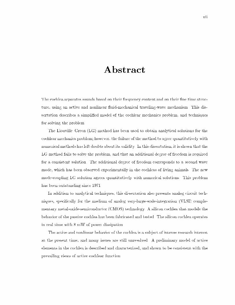
Abstract
The cochlea separates sounds based on their frequency content and on their �ne time struc-
ture, using an active and nonlinear uid-mechanical traveling-wave mechanism. This dis-
sertation describes a simpli�ed model of the cochlear mechanics problem, and techniques
for solving the problem.
The Liouville{Green (LG) method has been used to obtain analytical solutions for the
cochlear mechanics problem; however, the failure of the method to agree quantitatively with
numerical methods has left doubts about its validity. In this dissertation, it is shown that the
LG method fails to solve the problem, and that an additional degree of freedom is required
for a consistent solution. The additional degree of freedom corresponds to a second wave
mode, which has been observed experimentally in the cochleas of living animals. The new
mode-coupling LG solution agrees quantitatively with numerical solutions. This problem
has been outstanding since 1971.
In addition to analytical techniques, this dissertation also presents analog circuit tech-
niques, speci�cally for the medium of analog very-large-scale-integration (VLSI) comple-
mentary metal-oxide-semiconductor (CMOS) technology. A silicon cochlea that models the
behavior of the passive cochlea has been fabricated and tested. The silicon cochlea operates
in real time with 8 mW of power dissipation.
The active and nonlinear behavior of the cochlea is a subject of intense research interest
at the present time, and many issues are still unresolved. A preliminary model of active
elements in the cochlea is described and characterized, and shown to be consistent with the
prevailing views of active cochlear function.

viii

ix
Contents
1 Introduction 1
1.1 Review of Previous Work : : : : : : : : : : : : : : : : : : : : : : : : : : : : 2
1.2 Overview : : : : : : : : : : : : : : : : : : : : : : : : : : : : : : : : : : : : : 7
1.3 Original Contributions of the Present Work : : : : : : : : : : : : : : : : : : 8
2 The Biological Cochlea 10
2.1 Anatomy : : : : : : : : : : : : : : : : : : : : : : : : : : : : : : : : : : : : : 10
2.2 Function : : : : : : : : : : : : : : : : : : : : : : : : : : : : : : : : : : : : : : 18
2.3 Measurements : : : : : : : : : : : : : : : : : : : : : : : : : : : : : : : : : : : 23
2.4 Abstraction : : : : : : : : : : : : : : : : : : : : : : : : : : : : : : : : : : : : 27
3 Mathematical Models of Passive Cochlear Mechanics 31
3.1 Formulation of the Passive Two-Dimensional Problem : : : : : : : : : : : : 32
3.1.1 Hydrodynamics : : : : : : : : : : : : : : : : : : : : : : : : : : : : : : 33
3.1.2 Basilar-Membrane Boundary Condition : : : : : : : : : : : : : : : : 34
3.2 Review of Established Solution Techniques : : : : : : : : : : : : : : : : : : : 36
3.2.1 Numerical Solutions : : : : : : : : : : : : : : : : : : : : : : : : : : : 36
3.2.2 Exact Solution for a Uniform Cochlea : : : : : : : : : : : : : : : : : 37
3.2.3 Approximate LG Solution for a Nonuniform Cochlea : : : : : : : : : 46
3.3 New Solution Techniques : : : : : : : : : : : : : : : : : : : : : : : : : : : : 52
3.3.1 Higher-Order Calculation of Stapes Displacement : : : : : : : : : : : 52
3.3.2 The Mode-Coupling LG Solution : : : : : : : : : : : : : : : : : : : : 55
3.4 Discussion : : : : : : : : : : : : : : : : : : : : : : : : : : : : : : : : : : : : : 73

x
4 An Analog VLSI Model of Passive Cochlear Mechanics 80
4.1 Development of the Circuit Elements : : : : : : : : : : : : : : : : : : : : : : 80
4.1.1 The Fluid Subcircuit : : : : : : : : : : : : : : : : : : : : : : : : : : : 80
4.1.2 The Membrane Subcircuit : : : : : : : : : : : : : : : : : : : : : : : : 83
4.1.3 Variation of Parameters : : : : : : : : : : : : : : : : : : : : : : : : : 87
4.2 Characterization of the Cochlear Model : : : : : : : : : : : : : : : : : : : : 89
4.2.1 A Single Stage : : : : : : : : : : : : : : : : : : : : : : : : : : : : : : 91
4.2.2 The One-Dimensional Cochlear Model : : : : : : : : : : : : : : : : : 99
4.2.3 The Two-Dimensional Cochlear Model : : : : : : : : : : : : : : : : : 102
4.2.4 Comparison to Other Circuit Models : : : : : : : : : : : : : : : : : : 107
4.3 Analog VLSI Implementation : : : : : : : : : : : : : : : : : : : : : : : : : : 113
4.3.1 Resistor Circuit : : : : : : : : : : : : : : : : : : : : : : : : : : : : : : 113
4.3.2 Basilar-Membrane Circuit : : : : : : : : : : : : : : : : : : : : : : : : 114
4.3.3 Reduction of Parasitic Capacitance : : : : : : : : : : : : : : : : : : : 116
4.3.4 DC Operating Point : : : : : : : : : : : : : : : : : : : : : : : : : : : 118
4.3.5 Instrumentation, Fabrication, and Testing : : : : : : : : : : : : : : : 119
4.4 Summary : : : : : : : : : : : : : : : : : : : : : : : : : : : : : : : : : : : : : 119
5 Toward an Analog VLSI Model of Active Cochlear Mechanics 120
5.1 Review of Previous Active Models : : : : : : : : : : : : : : : : : : : : : : : 120
5.2 The Outer Hair Cell Model : : : : : : : : : : : : : : : : : : : : : : : : : : : 123
5.2.1 Mathematical Description : : : : : : : : : : : : : : : : : : : : : : : : 124
5.2.2 Analysis and Simulation : : : : : : : : : : : : : : : : : : : : : : : : : 125
5.2.3 The Circuit Model : : : : : : : : : : : : : : : : : : : : : : : : : : : : 127
5.3 Characterization of the Outer Hair Cell Circuit : : : : : : : : : : : : : : : : 129
5.4 Analog VLSI Implementation : : : : : : : : : : : : : : : : : : : : : : : : : : 131
5.5 Summary : : : : : : : : : : : : : : : : : : : : : : : : : : : : : : : : : : : : : 131
6 Summary and Conclusions 133
A Mathematica Code 135
A.1 Finite-Di�erence Method : : : : : : : : : : : : : : : : : : : : : : : : : : : : 135

xi
A.2 LG Method : : : : : : : : : : : : : : : : : : : : : : : : : : : : : : : : : : : : 139
A.3 Mode-Coupling LG Method : : : : : : : : : : : : : : : : : : : : : : : : : : : 141
A.4 Other Programs : : : : : : : : : : : : : : : : : : : : : : : : : : : : : : : : : : 143

xii

xiii
List of Figures
2.1 Anatomy of auditory periphery : : : : : : : : : : : : : : : : : : : : : : : : : 11
2.2 The unrolled cochlea : : : : : : : : : : : : : : : : : : : : : : : : : : : : : : : 11
2.3 Cochlea cross-section : : : : : : : : : : : : : : : : : : : : : : : : : : : : : : : 12
2.4 The organ of Corti : : : : : : : : : : : : : : : : : : : : : : : : : : : : : : : : 13
2.5 Hair cell detail. : : : : : : : : : : : : : : : : : : : : : : : : : : : : : : : : : : 15
2.6 Innervation of the hair cells. : : : : : : : : : : : : : : : : : : : : : : : : : : : 16
2.7 The auditory pathway. : : : : : : : : : : : : : : : : : : : : : : : : : : : : : : 17
2.8 Propagation of a wave : : : : : : : : : : : : : : : : : : : : : : : : : : : : : : 19
2.9 Detail of wave propagation. : : : : : : : : : : : : : : : : : : : : : : : : : : : 19
2.10 Frequency map on basilar membrane. : : : : : : : : : : : : : : : : : : : : : 21
2.11 Shearing movement of the basilar and tectorial membranes. : : : : : : : : : 22
2.12 Rhode place data. : : : : : : : : : : : : : : : : : : : : : : : : : : : : : : : : 24
2.13 Rhode nonlinear data. : : : : : : : : : : : : : : : : : : : : : : : : : : : : : : 25
2.14 Ruggero and Rich furosemide data. : : : : : : : : : : : : : : : : : : : : : : : 26
2.15 Sellick, Patuzzi, and Johnstone iso-response data. : : : : : : : : : : : : : : : 27
2.16 Summary of cochlear mechanics. : : : : : : : : : : : : : : : : : : : : : : : : 29
3.1 The physical model. : : : : : : : : : : : : : : : : : : : : : : : : : : : : : : : 32
3.2 The mathematical model. : : : : : : : : : : : : : : : : : : : : : : : : : : : : 35
3.3 The complex function tanh(kh). : : : : : : : : : : : : : : : : : : : : : : : : : 41
3.4 The tanh function and the three wave regions. : : : : : : : : : : : : : : : : 42
3.5 Comparison of LG and �nite-di�erence solutions. : : : : : : : : : : : : : : : 53
3.6 LG solution with improved calculation of stapes displacement. : : : : : : : 56

xiv
3.7 Validity of LG solution. : : : : : : : : : : : : : : : : : : : : : : : : : : : : : 58
3.8 Phase of uid pressure in numerical and LG solutions. : : : : : : : : : : : : 59
3.9 Example wavenumber trajectories. : : : : : : : : : : : : : : : : : : : : : : : 61
3.10 Behavior of P (x), Q(x) and R(x). : : : : : : : : : : : : : : : : : : : : : : : 64
3.11 Comparison of mode-coupling LG and Finite-Di�erence solutions. : : : : : : 66
3.12 Coupling coe�cients. : : : : : : : : : : : : : : : : : : : : : : : : : : : : : : : 67
3.13 Contribution of wave modes. : : : : : : : : : : : : : : : : : : : : : : : : : : 68
3.14 The infamous notch. : : : : : : : : : : : : : : : : : : : : : : : : : : : : : : : 69
3.15 The notch in the pressure pro�le. : : : : : : : : : : : : : : : : : : : : : : : : 70
3.16 Validity of mode-coupling LG solution : : : : : : : : : : : : : : : : : : : : : 72
3.17 Simpli�ed three-dimensional models : : : : : : : : : : : : : : : : : : : : : : 77
4.1 Resistive network. : : : : : : : : : : : : : : : : : : : : : : : : : : : : : : : : 82
4.2 Cochlea circuit with uid subcircuit shown explicitly. : : : : : : : : : : : : : 83
4.3 Analog VLSI circuit elements. : : : : : : : : : : : : : : : : : : : : : : : : : : 85
4.4 Variations of the basilar-membrane circuit. : : : : : : : : : : : : : : : : : : 86
4.5 Tilted bias lines. : : : : : : : : : : : : : : : : : : : : : : : : : : : : : : : : : 88
4.6 A single cochlea stage. : : : : : : : : : : : : : : : : : : : : : : : : : : : : : : 90
4.7 Poles and zeros of an isolated cochlea stage. : : : : : : : : : : : : : : : : : : 93
4.8 Reduction of stray capacitances with a driven shield. : : : : : : : : : : : : : 94
4.9 Voltage response of an isolated cochlea stage. : : : : : : : : : : : : : : : : : 95
4.10 Current response of an isolated cochlea stage. : : : : : : : : : : : : : : : : : 97
4.11 Saturating nonlinearity in a single stage. : : : : : : : : : : : : : : : : : : : : 98
4.12 One-dimensional cochlea circuit. : : : : : : : : : : : : : : : : : : : : : : : : 99
4.13 Amplitude responses of voltage taps. : : : : : : : : : : : : : : : : : : : : : : 100
4.14 Phase responses of voltage taps. : : : : : : : : : : : : : : : : : : : : : : : : : 101
4.15 Frequency responses of current taps. : : : : : : : : : : : : : : : : : : : : : : 103
4.16 Best frequency versus tap number : : : : : : : : : : : : : : : : : : : : : : : 104
4.17 Frequency response at di�erent amplitudes. : : : : : : : : : : : : : : : : : : 105
4.18 E�ect of driven shield on one-dimensional cochlea : : : : : : : : : : : : : : : 105
4.19 Fluid response at a �xed frequency. : : : : : : : : : : : : : : : : : : : : : : : 106
4.20 Real part of uid pressure at a �xed frequency. : : : : : : : : : : : : : : : : 108

xv
4.21 Magnitude of uid pressure at a �xed frequency. : : : : : : : : : : : : : : : 109
4.22 Comparison with the unidirectional-�lter-cascade model : : : : : : : : : : : 109
4.23 Comparison with the transmission-line model : : : : : : : : : : : : : : : : : 112
4.24 Mead's resistor circuit. : : : : : : : : : : : : : : : : : : : : : : : : : : : : : : 113
4.25 Detail of basilar-membrane circuit. : : : : : : : : : : : : : : : : : : : : : : : 115
4.26 The driven shield. : : : : : : : : : : : : : : : : : : : : : : : : : : : : : : : : 117
5.1 Yates' nonlinear feedback system. : : : : : : : : : : : : : : : : : : : : : : : : 126
5.2 Outer hair cell circuit : : : : : : : : : : : : : : : : : : : : : : : : : : : : : : 128
5.3 Response from a single outer-hair-cell circuit : : : : : : : : : : : : : : : : : 130
5.4 Detail of outer-hair-cell circuit. : : : : : : : : : : : : : : : : : : : : : : : : : 132

xvi

1
Chapter 1
Introduction
How do we hear? Can we build a machine that hears as well as we do? Our e�ortless
perception of sound belies the complex computations that are performed by the ear and
auditory pathway of the brain. Nature has evolved a highly e�cient system for processing
sound under constraints that were important for survival of the species|namely, that the
system must provide accurate and useful information about the environment, in real time,
with a minimum consumption of power, with small size, and with subcomponents that may
be imperfect or even nonoperational. In addition, the system must be capable of operating
on signals that are noisy and ambiguous with a large dynamic range. This set of constraints
imposes severe limitations on the form of the system.
The task of building arti�cial systems that perform as well as biological systems has
proven to be extremely di�cult. For many years, engineers have attempted to build ma-
chines to understand speech, to interpret visual scenes, or to manipulate objects, with
limited success, despite huge advances in arti�cial information-processing technology. We
are not limited by our technological substrate; rather, we are limited by our lack of under-
standing of the organizational principles at the heart of the robust and e�cient biological
sensory systems.
In the present work, the biological system under study is the cochlea, the sense organ
of hearing. The cochlea is a spiral tube �lled with uid; a exible membrane runs down its
length. The cochlea uses an active and nonlinear traveling-wave mechanism and motion-
2
sensitive hair cells on the exible membrane to transform sound into a time-varying pattern
of excitation on the �bers of the eighth cranial nerve.
If we truly understand the organizing principles of the biological cochlea, we should be
able to build an arti�cial cochlea based on those principles. But in what medium should
the arti�cial cochlea be implemented? For highly constrained systems such as this one, the
choice of implementation technology is critical; the primary requirements of low-power and
real-time operation eliminate many candidate technologies, such as software implementation
on a conventional digital computer or digital-signal-processing chip.
Complementarymetal-oxide-semiconductor (CMOS) very-large-scale-integration (VLSI)
technology has emerged as the most dense, power-e�cient, and inexpensive information-
processing technology currently available. Mead has pioneered the application of analog
VLSI CMOS technology to the construction of special-purpose chips that model the sensory
and neural processing of biological systems. By exploiting the physics of the transistor|
particularly the subthreshold characteristics|Mead and his collaborators have built sophis-
ticated neuromorphic systems that operate in real time with power consumption orders of
magnitude lower than that of conventional digital implementations [71, 69, 66, 29].
This dissertation is an investigation of the biology, physics, and mathematics of cochlear
mechanics, with the goal of understanding the physical processes that underly the observed
cochlear behavior. A working silicon cochlea has been built in analog VLSI CMOS technol-
ogy.
1.1 Review of Previous Work
The cochlea is a complex three-dimensional uid-mechanical structure that separates sounds
on the basis of their frequency content and �ne time structure, and that encodes the infor-
mation as impulses on the 25,000 �bers of the eighth cranial nerve.
A readable account of the history of auditory anatomy and function is given by Carterette
[10], covering the period from the ancient Greeks to modern day. Prior to the mid-1800s,
the studies were primarily anatomical, and identi�ed the major features of the peripheral
auditory system, such as the eardrum, bones of the middle ear, and the cochlea. The
coiled basilar membrane was �rst described by Du Verney in 1683 [119]. By the mid-1800s,

3
improved microscopes and chemical tissue �xatives had enabled a description of the �ner
structures of the cochlea. Reissner (1851) [88], Corti (1851) [12], and Deiters (1860) [23]
applied the new technologies and discovered the cochlear structures now named after them.
Nuel (1872) [82], Retzius (1884) [89], and Held (1897) [42] mapped out the paths of the
auditory-nerve �bers and identi�ed the terminations of those �bers on the hair cells. At
this point, the hair cells were identi�ed as the true sensory elements.
An early theory of hearing by Helmholtz in 1863 [123] suggested a parallel bank of
resonators as the mechanism for frequency selectivity; the transverse �bers of the basilar
membrane were supposed to act as the resonant elements. Other theories abounded, in-
cluding the so-called telephone and standing-wave theories; the great hearing researcher von
B�ek�esy wrote [122, p. 471], \Because for more than a century no numerical values con-
cerning the mechanical properties of the cochlear partition were available, there were no
restrictions on the imagination, and probably every possible solution of the problem was
proposed." The pioneering work by von B�ek�esy from 1924 to 1960 [122], for which he re-
ceived a Nobel Prize in 1961, used new microdissection techniques, a light microscope, and
stroboscopic illumination to observe the propagation of traveling waves in excised cadaver
cochleas in response to a pure tone. Passive one-dimensional models [137, 87] were capable
of qualitative agreement with von B�ek�esy's data, and established a theoretical basis for
the traveling-wave mechanism, although there was considerable debate over whether waves
should be considered long or short with respect to the diameter of the cochlear duct.
von B�ek�esy's studies indicated that the vibrations were linear and were not sharply
tuned; that is, a wide range of frequencies could elicit a signi�cant response from a given
place on the basilar membrane. However, in 1965, Kiang and colleagues measured sharply
tuned responses of single auditory-nerve �bers [51]. In 1973, Evans and Wilson observed
that the sharpness of the neural responses depended on the physical condition of the animal
subject [28]. These observations led to the proposal of a physiologically vulnerable \second
�lter" [28], located conceptually between the basilar-membrane motion and the responses
of the a�erent neurons, that would somehow provide the missing frequency selectivity.
Until 1967, von B�ek�esy was the only person to have made direct measurements of
basilar-membrane motion. The sensitive M�ossbauer technique was used to measure basilar-
membrane motion in living animals by Johnstone and Boyle in 1967 [45], and by Rhode

4
in 1970 [90, 91]. In the M�ossbauer technique, a small radioactive source is placed on the
basilar membrane, and its velocity is inferred by measurement of the Doppler shift of the
emitted gamma radiation. Rhode's data were more sharply tuned than the cadaver data
of von B�ek�esy, and also showed a compressive amplitude nonlinearity. Rhode showed that
the sharp tuning was dependent on the health and experimental condition of the animal
subject. Finally, Rhode observed the presence of an unexpected vibration mode, which
caused a plateau in the amplitude and phase measurements at high frequencies.
The improved data prompted tremendous activity in theoretical models. In the 1970s,
the cochlea was recognized as a wave-propagation medium in which the physical parameters
varied slowly; thus, the mathematical analysis techniques developed by Liouville [61] and
Green [40] in the mid-1800s could be applied to the problem. The Liouville{Green (LG)
method was �rst applied to cochlear mechanics problems by Steele in 1974 [109]. Closed-
form LG solutions were found for the one-dimensional short-wave model by Siebert in 1974
[103], and for the one-dimensional long-wave model by Zweig, Lipes, and Pierce in 1976 [134].
The LG method was extended to two- and three-dimensional models by Steele in 1974 [109],
by Steele and Taber in 1979 [112, 111], and by Taber and Steele in 1981 [118], and was further
developed by de Boer and Viergever in 1982 and 1984 [21, 22]. Several numerical solutions
for the two-dimensional model were proposed|notably, the �nite-di�erencemethod of Neely
[79], and the integral-equation method of Allen [3]. The LG method for the two-dimensional
model was shown by Steele and Taber to agree qualitatively with the numerical solutions,
except for the high-frequency plateau [112]. de Boer and Viergever observed that the
high-frequency plateau was related to the multiple roots of the dispersion relation in the
LG formulation [21], but did not give a physically sound procedure for correcting the LG
method. Three-dimensional �nite-element solutions were computed in 1987 by Kagawa and
colleagues [46]. However, no selection of physical parameters was found for any of the models
that was capable of matching the existing biological data quantitatively, in both amplitude
and phase. de Boer concluded [16, 17] that some active region with negative mechanical
damping would be required to match the sharp tuning of modern measurements.
In 1982, Sellick, Patuzzi, and Johnstone compared basilar-membrane isovelocity data
with auditory-nerve tuning curves from a live guinea pig, and showed that the basilar-
membrane vibration could account almost completely for the sharp tuning of the auditory-

5
nerve response [101]. Their �ndings called o� the long search for the \second �lter" that
would reconcile the sharpness of the basilar-membrane response and the neural tuning
curves. Careful animal preparations and the improved sensitivity of modern measurement
techniques are usually given credit for resolving the issue [14, p. 213], but there is a
much more subtle point here. Rhode's measurements from 11 years earlier were made
with the same sensitive technique and careful animal preparation. What was missing at
that time was an understanding of the e�ect of the compressive nonlinearity on isoresponse
measurements|namely, to render them incomparable with isointensity measurements, as
emphasized by Lyon and colleagues [65, 66, 63], and reiterated by Ruggero [94, p. 450].
Perhaps the greatest contribution of Sellick and colleagues in 1982 was to collect isovelocity
data, which could then be compared legitimately with the neural tuning curves. Another
factor in this story was the fact that the compressive amplitude nonlinearity, observed by
Rhode in 1971, could not be con�rmed in other species for nearly a decade [92].
Throughout the 1970s and 1980s, evidence began to accumulate that the cochlea was
active as well as nonlinear, and that these phenomena were related. The nonlinear e�ects
included distortion products and two-tone suppression [96]. The idea of active processes
in the cochlea was �rst suggested by Gold in 1948 [38]. Compelling evidence for active
processes was given by Kemp in 1978 [48] in the form of objective tinnitus (sustained
ringing in the ears) and oto-acoustic emissions (sounds emanating from the ears). Many re-
searchers have regarded the role of the active processes primarily as a frequency-sharpening
mechanism; Lyon [63] and Lyon and Mead [67] have emphasized that the active processes
function primarily as an automatic gain control, allowing the ampli�cation of sounds that
would otherwise be too weak to hear.
A growing majority of the hearing-research community now accepts the outer hair cells
as the cause of the active nonlinearity. Unlike the inner hair cells, which act as sensory
transducers involved in the transmission of information to the brain, the outer hair cells act
as tiny muscles, adding energy to the traveling wave under the high-level control of signals
from the brain.
In the 1980s and early 1990s, research has shifted toward an understanding of the active
outer hair cells. Brownell [9] and Evans and colleagues [26] have identi�ed force-generating
and force-stimulating mechanisms in the outer hair cells. Ruggero and Rich [95] have shown

6
that mechanically active cells in the organ of Corti|very probably the outer hair cells|are
responsible for the responsiveness of the basilar-membrane vibration. Santos-Sacchi [97] has
given evidence that outer hair cells are capable of electrically induced vibrations at rates
up to 1 kHz, and possibly higher. Other researchers [77, 16, 80, 75, 34, 35, 55, 130, 133]
are trying to understand the functional role of active processes in the wave-propagation
mechanism. Currently, there is no consensus on the detailed mechanism by which the outer
hair cells amplify the traveling wave. However, most models assume that the outer hair cells
respond to stimulation by pushing on the basilar membrane with a frequency- and position-
dependent delay. Under the right conditions, the forces generated by the outer hair cells
act in phase with the velocity of the basilar membrane, resulting in an ampli�cation of the
vibration.
To simplify analysis or to reduce simulation times, many researchers are investigating
active processes in one-dimensional models. However, it appears that the two-dimensional
active model is the simplest model capable, in principle, of capturing the essence of cochlear
uid mechanics; the choice of this level of abstraction will be justi�ed in Chapter 2.
The �rst electrical analog of the cochlea was the transmission-line model, proposed by
Peterson and Bogert as a conceptual aid in 1950 [85]. Analog simulation techniques reached
a pinnacle in the 1950s [47], however, as the computing power of digital computers exploded
in the 1950s and 1960s, analog simulation fell out of favor. A few workers, particularly
Stewart [114, 115] and Zwicker [135, 136] have built analog electrical cochlear models out of
discrete components. Lechner has built a sophisticated hydromechanical model with active
elements [58].
There is now a quiet revival of the �elds of analog simulation and analog computation, led
by Mead, fueled by the need for real-time performance on demanding sensory perception
tasks, and by the high densities, low cost, and low power consumption of analog VLSI
technology. Lyon and Mead [66] have argued that the wave-propagation mechanism of
the cochlea can be modeled by a cascade of second-order low-pass �lter sections. Like
the biological cochlea, their cascade propagates a forward-going wave that slows down,
decreases in wavelength, and suddenly dies out. No re ections are possible in the cascade;
the enforced unidirectionality models only the forward-going waves normally observed in
the real cochlea. By tuning each section to have a small resonant frequency band, in which

7
the gain from input to output is slightly larger than unity, Lyon and Mead found that
active processes in the cochlea could be modeled. Their model is not sharply tuned; no
single �lter stage has a highly resonant response. Instead, a high-gain e�ect is achieved
by the cumulative e�ect of many low-gain stages, similar to the real cochlea. Their model
was implemented in micropower analog subthreshold VLSI [71], and has many important
similarities to the present work.
1.2 Overview
This dissertation describes the implementation of a realistic model of cochlear wave propa-
gation in analog VLSI CMOS technology, based on a detailed understanding of the operation
of the biological cochlea. At the philosophical core of the work is the conviction that engi-
neering insights can come frommany diverse disciplines: anatomy, physiology, mathematical
analysis, computer simulation, and the construction of models in a physical medium. Each
of these disciplines has played an indispensable role in the present work.
In Chapter 2, the anatomy and function of the biological cochlea are reviewed. The
landmark measurements that have shaped the modern understanding of the mechanisms
of hearing are quoted. Finally, a simpli�ed two-dimensional active model is justi�ed as a
suitable abstraction for further study.
In Chapter 3, the two-dimensional passive model is described. The established solution
methods are described, with emphasis on the numerical �nite-di�erence method [78], and
the analytical LG method [109, 112, 21, 22]. The two solutions are compared for the same
physical parameters; the LG solution is found to break down near the resonance point. A
detailed study of this phenomenon indicates that a second wave mode is required to solve
the problem. A new solution, called the mode-coupling LG solution, is introduced, and
is found to agree quantitatively with the �nite-di�erence solution. A new formula for the
stapes displacement improves the accuracy of the LG solutions when the wavelength at
the stapes is very long. Mathematica code for implementing the �nite-di�erence, LG, and
mode-coupling LG solutions is provided in Appendix A. Finally, the implications of the
model parameters for a physical implementation are discussed.
In Chapter 4, a new analog VLSI model of the passive cochlea is introduced. The

8
model uses a resistive network to model the cochlear uid, and a bank of special-purpose
circuits to model the basilar membrane. The circuits are characterized in a single stage,
in a one-dimensional model, and in the full two-dimensional model. Nonlinearities and
parasitic capacitances are found to play an important role in the silicon implementation.
The circuit is capable of replicating features of the two-dimensional conceptual model,
including the transition from long-wave to short-wave propagation, and the emergence of
the second wave mode predicted by the mode-coupling LG solution of Chapter 3. The
model is compared to the �lter cascade analog VLSI model of Lyon and Mead [66], and
to the classical transmission-line model [85]. A detailed transistor-level description of the
circuit concludes Chapter 4.
In Chapter 5, an outer-hair-cell circuit model is introduced, based on the conceptual
active-sti�ness model of Mountain, Hubbard, and McMullen [77]. The circuit is shown to
generate the appropriate delayed signal as required by the conceptual model; however, the
method for feeding the signal back to the basilar membrane is still under development.
A summary and conclusions are given in Chapter 6.
1.3 Original Contributions of the Present Work
The original contributions of the present work include the mode-coupling LG solution,
introduced in Section 3.3.2, which predicts the cochlear vibration mode �rst observed by
Rhode in 1971 [91]. This problem has been outstanding for over 20 years.
An improved calculation for the stapes displacement is proposed in Section 3.3.1, based
on including higher-order terms that are commonly neglected. This simple improvement
corrects a large discrepancy between the simple LG solution and the numerical solutions.
This problem has been outstanding for over 10 years.
An improved validity condition for the LG solution is introduced in Section 3.3.2; it
identi�es where the simple LG method fails.
The combination of these three theoretical contributions leads, for the �rst time, to
an analytical formulation that is capable of qualitative and quantitative agreement with
numerical solutions.
The entire analog VLSI cochlear model is an original contribution. In particular, the

9
use of a resistive network to model the incompressible inviscid uid, with active circuitry
to model the basilar membrane, is novel.
The outer-hair-cell model is based on the conceptual active-sti�ness model of Mountain,
Hubbard and McMullen [77]. However, its implementation in analog VLSI is novel.

10
Chapter 2
The Biological Cochlea
The cochlea is a highly developed and complex mechanical sensory system. Its function is
to convert a single time-varying pressure signal into a time-varying pattern of excitation on
the approximately 25,000 �bers of the eighth cranial nerve. In this chapter, the anatomy
and basic function of the cochlea are described, and the landmark measurements that
have shaped the modern understanding of cochlear operation are quoted. Finally, a simple
abstract model that captures the essential features of cochlear operation is described.
2.1 Anatomy
The general description of the anatomy is based on the treatments of Dallos [13], Evans [27],
Kessel and Kardon [50], M�ller [74], and Shepherd [102]. Figure 2.1 shows the anatomy
of the human auditory periphery. Sound waves travel down the canal or external auditory
meatus, and vibrate the eardrum or tympanic membrane. On the other side of the eardrum
is the internal auditory meatus, an air-�lled cavity that leads to the nasopharynx via the
Eustachian tube, which opens during swallowing to equalize pressure across the eardrum.
Vibrations of the eardrum couple into the small bones or ossicles of the middle ear, called
the hammer or malleus, anvil or incus, and stirrup or stapes. The footplate of the stapes
presses on the oval window, an opening in the vestibule of the inner ear. Vibration of the
stapes causes waves to travel in the uid inside the vestibule and the cochlea. The round

11
TympanicMembrane
MalleusIncus
Stapes
Oval Window
Round Window
Cochlea
Cochlear Nerve
Eustachian Tube
External Auditory Meatus
Temporal Bone
Vestibule
SemicircularCanals
Parotid Gland
Pinna
Internal Auditory Meatus
Figure 2.1 Anatomy of the human auditory periphery. Adapted from
Kessel and Kardon [50].
Stapes
Oval Window
Round Window
Basilar Membrane
Helicotrema
Bony Shelf
Scala Tympani
Scala Vestibuli
Reissner's Membrane
Scala Media
Base
Apex
Figure 2.2 The unrolled cochlea, simpli�ed to emphasize the bony shelf
and widening of the basilar membrane. Adapted from Cole and Chadwick
[11].

12
Scala Vestibuli
Scala Tympani
TectorialMembrane
Basilar Membrane
Spiral Ganglion
Reissner's Membrane
Organ of Corti
Bony Shelf
Bony Wall
Stria Vascularis
Spiral Ligament
ScalaMedia
Spiral Limbus
Figure 2.3 Cross-section through the cochlea. Adapted from Kessel and
Kardon [50].
window allows pressure relief for the incompressible cochlear uid.
The middle ear provides a mechanical advantage to allow the pressure uctuations of
the air to couple energy e�ciently into movement of the uid-and-membrane structure of
the cochlea. However, the middle ear is not a simple air-to-water impedance matcher,
as is commonly believed; to characterize it as such is to assume incorrectly that acoustic
(compressional) waves are propagated in the cochlear uid. Rather, waves are propagated
by the combined movement of the incompressible cochlear uid and the membranes inside
the cochlea, so the middle ear is matching the impedances of the air and the sti�est part
of the membrane. A discussion of the historical confusion surrounding this subtle point is
given by Schubert [99].
The cochlea and vestibular apparatus are commonly believed to have evolved from the

13
TectorialMembrane
Basilar Membrane
Pillar Cells
InternalSpiral Tunnel
Dieter's Cells
Hensen's Cells
Cells of Claudius
Inner Hair Cell
Outer Hair Cell
Nerve Fibers
Reticular Lamina
HabenulaPerforata
Spiral Vessel
Figure 2.4 The organ of Corti, with the tectorial membrane partially cut
away. Adapted from Kessel and Kardon [50].
lateral line organ of �shes [102, pp. 309-310]. In humans, the cochlea is about 35 mm long
and about 2 mm in diameter. If the spiral cochlea structure could be unrolled, it would
appear as a long uid-�lled tube, with the basilar membrane and Reissner's membrane
running down its length, as shown schematically in Figure 2.2. The membranes and the
bony shelf or spiral osseus lamina subdivide the cochlea into three major compartments or
scalae|namely, the scala vestibuli, scala media, and scala tympani|running from the base
of the cochlea to the apex.
The basilar membrane and Reissner's membrane run nearly the length of the cochlea.
The scala media terminates near the apex of the cochlea. At the apex of the cochlea, the
basilar membrane terminates, and a small hole in the bony shelf, called the helicotrema,
allows the scalae vestibuli and tympani to join. The helicotrema allows for equalization of

14
pressure and ionic concentration of the uid in the scalae vestibuli and tympani.
The basilar membrane is not an isotropic stretched membrane; it consists of long, thin,
beamlike �bers running across its width [44]. There is virtually no direct mechanical cou-
pling from one �ber to the next. The basilar membrane is sti� and narrow (about 100 �m)
near the base, and exible and wide (about 500 �m) near the apex, with a smooth transi-
tion along its length. The sti�ness of the basilar membrane decreases by at least a factor
of 100 from base to apex, in an approximately exponential fashion [13, p. 136]. Reissner's
membrane is light, thin, and very exible. It serves no mechanical purpose; its function is
to provide ionic isolation between the scalae media and vestibuli.
The uid contained in the scalae vestibuli and tympani is called perilymph; it is high
in sodium content and low in potassium content, similar to interstitial uid. The scala
media is �lled with endolymph, a uid that has a low sodium concentration but is rich in
potassium. The di�erence in ionic concentration between the endolymph and perilymph is
maintained by the dense capillary network called the stria vascularis, shown in Figure 2.3.
The stria vascularis is the site of intense metabolic activity, which necessarily requires ac-
cess to the bloodstream for nutrients and waste disposal. The purpose of this sophisticated
arrangement is to maintain the electrical potential di�erence, called the endocochlear po-
tential, between the perilymph and endolymph. The endocochlear potential acts as a quiet
power supply for the hair cells in the organ of Corti [15, 131]; these hair cells are sensitive
to tiny movements, and must be isolated from the noise of the circulatory system. A small
blood vessel, called the spiral vessel, also runs beneath the basilar membrane, as shown in
Figure 2.4, but no capillaries are extended into the organ of Corti.
When the hair cells of the organ of Corti draw power from the stria vascularis in response
to an input sound, small uctuations in the endocochlear potential can be measured. These
uctuations are called the cochlear microphonic, since the measured voltage waveform is an
approximate replica of the sound itself.
The tectorial membrane is a transparent, noncellular, exible, gelatinous mass that is
situated between the organ of Corti and Reissner's membrane. It is suspended above the
organ of Corti from the spiral limbus, which is an enlargement of the cell lining of the
cochlear interior. The uid-�lled space beneath the tectorial membrane and enclosed by
the spiral limbus and organ of Corti is called the internal spiral tunnel or spiral sulcus. The

15
Tectorial Membrane
Stereocilia
Tectorial Gap
Inner Hair Cell
E�erent
A�erent
Synapse
Nucleus
Outer Hair Cell
SynapticVesicles
Fiber
Fiber
Axo-DendriticSynapse
Figure 2.5 Detail of the inner and outer hair cells, showing their relation-
ship to the tectorial membrane and to the nerve �bers. The stereocilia tips
of the outer hair cells are embedded in the tectorial membrane, whereas the
stereocilia of the inner hair cells are free to move in the tectorial gap. The
hair cells and nerve �bers communicate via chemical synapses. Although most
nerve �bers make synaptic connections directly with the hair cell bodies, the
e�erent �bers that innervate the inner hair cells virtually always form axo-
dendritic synapses on the a�erent �bers, as shown. Adapted from Bodian [7].
slim region between the tectorial membrane and the organ of Corti is called the tectorial
gap or subtectorial space.
The organ of Corti is shown in Figure 2.4. It resides on top of the basilar membrane,
and contains one row of inner hair cells, and three to �ve rows of outer hair cells, so named
for their position with respect to center of the spiral. There are about 3000 inner hair
cells and about 9000 outer hair cells, spaced about 10 �m apart. The hair cells are rigidly
attached to the basilar membrane by the supporting Dieter's cells and the pillar cells. The
Dieter's cells have processes that extend upward to hold the tops of the outer hair cells; the

16
Base Apex
Inner Hair Cell
Outer Hair Cell
Spiral Ganglion
5%85% 8%
2%
� 0.6 mm
Contra
Ipsi
Cell
Figure 2.6 Innervation of the hair cells. The e�erent �bers from the
contralateral and ipsilateral olivocochlear bundles are labeled \Contra" and
\Ipsi," respectively. The percentages indicate the representation of �bers of
the given type in the cochlear nerve. The majority of �bers are a�erent �bers
from inner hair cells. Adapted from Spoendlin [107].
resulting rigid upper surface of the organ of Corti is called the reticular lamina.
All the hair cells have stereocilia, or �ne �laments, that extend upward into the tectorial
gap from the reticular lamina. There are many important di�erences between the inner hair
cells and the outer hair cells, as shown in Figure 2.5. The outer hair cells vary in length
between about 30 �m at the base to about 70 �m at the apex. The length of the stereocilia
of the outer hair cells is also graded, increasing from about 4 �m at the base to about 8
�m at the apex. The ends of the tallest stereocilia of the outer hair cells are embedded
�rmly in the tectorial membrane, whereas the stereocilia of the inner hair cells are free to
move in the uid in the tectorial gap. The stereocilia are arranged in a V or W formation
for the outer hair cells, and in a shallow curve for the inner hair cells. The outer hair cells
are tall, slim, and sti�, with �ne tensile �laments that wrap around the cell body, to form
a kind of skeleton structure [9]. In addition, the outer hair cell walls are known to contain
actin, which is the contractile protein of muscle. The outer hair cells make contact with the

17
Cochlea
CochlearNucleus
Brainstem
Midbrain
Thalamus
Cortex Cortex
Thalamus
Midbrain
Brainstem
NucleusCochlear
Cochlea
Figure 2.7 The auditory pathway of the brain, highly simpli�ed. Ascending
connections are shown as thick lines, descending connections are shown as
thin lines. The majority of e�erent connections to the cochlea are from the
olivocochlear bundle on the contralateral side of the brainstem.
supporting cells only at their tops and bottoms; most of the length of the outer hair cell is
free to move. By contrast, the inner hair cells are short, round, and exible, with no tensile
skeleton structure. They have an approximately uniform size, regardless of their position
along the length of the cochlea, and they are bound tightly by the supporting cells.
The relationship between the hair cells and the nerve �bers is shown in Figure 2.5. Nerve
�bers that carry signals to the brain are a�erent �bers, whereas those carrying signals from
the brain are e�erent �bers. The majority of nerve �bers that make connections to the outer
hair cells are e�erent, whereas the majority of nerve �bers that make connections to the
inner hair cells are a�erent. Connections from the hair cells to the a�erent �bers are made
by excitatory chemical synapses; connections from the e�erent �bers to the hair cells are
made by inhibitory synapses [74, p. 70]. Synaptic vesicles in the transmitting cell release
neurotransmitter into the synaptic cleft between the two cells, causing an in ux of current
into the receiving cell.
The most common patterns of innervation of the hair cells are shown schematically in

18
Figure 2.6. The a�erent connections from the hair cells to the brain are made via the spiral
ganglion cells. A single inner hair cell may make a�erent connections to as many as 10 or
20 spiral ganglion cells; each of those spiral ganglion cells communicates only to that one
inner hair cell. However, many outer hair cells make a�erent connections to a single spiral
ganglion cell. As shown in Figure 2.6 [107], a�erent connections to inner hair cells at one
location are associated with a�erent connections to outer hair cells in a region that extends
a short distance toward the basal end of the cochlea.
The e�erent connections to the outer hair cells are made by nerve �bers from the olivo-
cochlear bundle in the superior-olive region of the brainstem. The majority of the e�erent
connections come from the crossed, or contralateral, bundle, with the remainder coming
from the uncrossed, or ipsilateral, bundle. A few e�erent �bers innervate the inner hair
cells, virtually always forming axo-dendritic synapses on the a�erent �bers [14], as shown in
Figure 2.5. A highly simpli�ed diagram of the neural connections in the auditory pathway
is shown in Figure 2.7. A summary of the auditory pathway is given by Shepherd [102].
2.2 Function
The functional input to the cochlea is the stapes movement, which is a high-�delity replica
of the sound pressure in the air outside the ear. We are now concerned with how the cochlea
performs its encoding of the input signal into nerve impulses on the cochlear nerve.
Sinusoidal movement of the stapes causes waves to propagate down the uid and mem-
brane structure of the cochlea, as shown in Figure 2.8. The wave is not carried solely by
compression of the uid, since the cochlear uid is essentially incompressible at audio fre-
quencies; rather, the wave is propagated by the combined movement of the uid and the
membrane. Since the uid cannot be compressed, conservation of uid mass dictates that
the round window must move in opposition to the stapes, as measured experimentally by
von B�ek�esy [122].
At the basal end of the cochlea, the basilar membrane is narrow and sti�, so the
membrane-displacement waves propagate quickly with long wavelength. As the wave travels
down the cochlea, the sti�ness of the membrane decreases, so the waves slow down, become
shorter, and increase in amplitude. At some point, called the best place for the given input

19
Figure 2.8 Propagation of a wave down the cochlea, for a �xed input fre-
quency, viewed at one moment. Since Reissner's membrane has no mechanical
e�ect, it is not shown, and cochlea is treated as though there were only the
scalae vestibuli and tympani.
Membrane Displacement
Fluid Pressure
Long-Wave Short-Wave Cut-Off
Figure 2.9 Detail of wave propagation, showing the membrane displace-
ment and uid pressure along a vertical slice through the lower chamber, for
a sinusoidal stapes vibration. The amplitude of the membrane displacement
wave is small near the base, reaches a peak at the best place, and dies out
quickly in the cut-o� region. Deviations in uid pressure from the resting
pressure are shown as dark or light deviations from gray. The amplitude of
the uid pressure wave is large near the base, and gradually decays through
the long-wave and short-wave regions, and dies out quickly in the cut-o� re-
gion. In the short-wave region, the amplitude of the pressure wave decreases
approximately exponentially away from the partition.

20
frequency, the membrane will vibrate with maximum amplitude. Beyond the best place,
the basilar membrane becomes too exible and highly damped to support wave propagation
at the given frequency, and the wave energy dissipates rapidly.
The membrane displacement and uid pressure in the lower chamber are shown schemat-
ically in Figure 2.9. The wave is said to be in the long-wave region when its wavelength
is long with respect to the height of the duct. In this region, the uid particle motion is
constrained to be essentially horizontal, like a wall of uid moving back and forth in a pipe.
When the wavelength becomes short with respect to the height of the duct, the wave is said
to have entered the short-wave region. At this point, the wave propagates more like ripples
on the surface of a deep pond, where the uid particles trace out elliptical trajectories, with
greater amplitude near the surface. Finally, the wave dies out in the highly damped cut-o�
region.
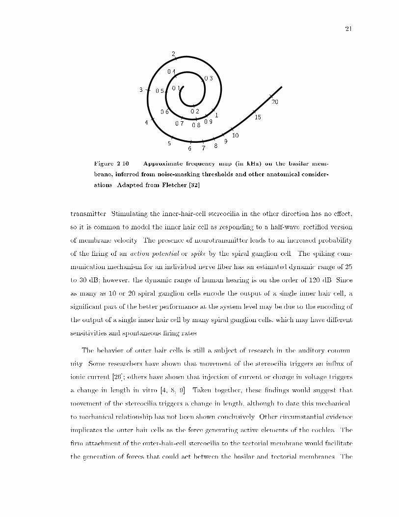
The position of maximum displacement of the basilar membrane varies approximately
logarithmically with the frequency of the input, for frequencies above about 1 kHz [67].
Frequencies lower than 1 kHz are more compressed along the length of the cochlea, as
shown in Figure 2.10.
The coiling of the biological cochlea has no signi�cant e�ect on the traveling wave
[62, 113]. The primary purpose of the coiling appears to be to save space.
The e�ect of basilar-membrane displacement on the stereocilia of the hair cells is shown
in Figure 2.11. In this commonly accepted view, attributed to Ter Kuile [13, p. 144],
movement of the basilar membrane results in a shearing movement of the reticular lamina
against the gelatinous tectorial membrane. For small displacements, the degree of shear|
and hence the bending of the outer-hair-cell stereocilia, which are attached to the tectorial
membrane|is proportional to the displacement of the membrane. Since the inner-hair-cell
stereocilia are not attached to the tectorial membrane, they are bent by a force due to viscous
drag as they move with respect to the uid in the tectorial gap; this force is proportional
to the velocity of basilar membrane. So, to a �rst order, outer-hair-cell stereocilia are
stimulated in proportion to membrane displacement, whereas inner-hair-cell stereocilia are
stimulated in proportion to membrane velocity.
Stimulation of the inner-hair-cell stereocilia in one direction triggers the in ux of ionic
currents into the hair cell, which depolarizes the membrane and leads to a release of neuro-
21
0.1
0.2
0.30.4
0.5
0.6
0.7 0.80.9
1
2
3
4
56 7 8
910
15
20
Figure 2.10 Approximate frequency map (in kHz) on the basilar mem-
brane, inferred from noise-masking thresholds and other anatomical consider-
ations. Adapted from Fletcher [32].
transmitter. Stimulating the inner-hair-cell stereocilia in the other direction has no e�ect,
so it is common to model the inner hair cell as responding to a half-wave{recti�ed version
of membrane velocity. The presence of neurotransmitter leads to an increased probability
of the �ring of an action potential or spike by the spiral ganglion cell. The spiking com-
munication mechanism for an individual nerve �ber has an estimated dynamic range of 25
to 30 dB; however, the dynamic range of human hearing is on the order of 120 dB. Since
as many as 10 or 20 spiral ganglion cells encode the output of a single inner hair cell, a
signi�cant part of the better performance at the system level may be due to the encoding of
the output of a single inner hair cell by many spiral ganglion cells, which may have di�erent
sensitivities and spontaneous �ring rates.
The behavior of outer hair cells is still a subject of research in the auditory commu-
nity. Some researchers have shown that movement of the stereocilia triggers an in ux of
ionic current [26]; others have shown that injection of current or change in voltage triggers
a change in length in vitro [4, 8, 9]. Taken together, these �ndings would suggest that
movement of the stereocilia triggers a change in length, although to date this mechanical-
to-mechanical relationship has not been shown conclusively. Other circumstantial evidence
implicates the outer hair cells as the force-generating active elements of the cochlea. The
�rm attachment of the outer-hair-cell stereocilia to the tectorial membrane would facilitate
the generation of forces that could act between the basilar and tectorial membranes. The

22
De ection
RelativeMotion
(a) (b)
Figure 2.11 Shearing movement of the basilar and tectorial membranes,
when the basilar membrane is displaced. The outer-hair-cell stereocilia are
bent in proportion to membrane displacement. Adapted from Miller and Towe
[73].
outer hair cells are located centrally in the organ of Corti, where the basilar membrane
undergoes its largest excursion, and hence are favorably positioned to exert forces on the
basilar membrane. Under the right conditions, it is likely that the outer cells act so as to
add energy to the traveling wave, to amplify sounds that would otherwise be too weak to
be encoded e�ectively by the inner hair cells and spiral ganglion cells.
Under some conditions, the active outer hair cells can become unstable, leading to
oscillations. The resulting ringing in the ears is known as tinnitus. The oscillations can
cause waves to travel both forward and backward along the cochlea. The backward-going
waves can couple energy out through the bones of the middle ear to the eardrum, which then
broadcasts sound out of the ear [132]. Other spectacular artifacts of the active processes
include the Kemp echo, a re ected sound that follows stimulation by a click or tone burst
[48].
Most active cochlear models assume that outer hair cells are capable of applying forces
to the basilar membrane at frequencies that span essentially the entire range of hearing. The
assumption of fast motility is being checked experimentally, and evidence is accumulating
that the outer hair cells are capable of changing length at frequencies at least up to 1 kHz
[97], and possibly higher [43].
Note that the detailed mechanisms by which the inner hair cells are stimulated, and by
which the outer hair cells may in uence the wave propagation in vivo, are still unknown.

23
This fascinating subject is known as cochlear micromechanics. Ter Kuile's shearing mecha-
nism is one example of a micromechanical model; other interesting micromechanical models
include models of viscous ow through the subtectorial gap from the spiral sulcus [108], and
preferential bending of the basilar membrane in di�erent regions [118, 56].
2.3 Measurements
In 1971, Rhode reported the �rst in vivo measurements of the amplitude and phase of
basilar-membrane motion using the M�ossbauer technique [91]. Rhode also measured the
motion of the malleus, and hence was able to present a malleus-to-basilar-membrane transfer
function.
Rhode measured frequency responses at two di�erent positions on the basilar membrane,
x1 and x2, as shown in Figure 2.12. Each curve shows a characteristic peak at its best
frequency. The position x1 is 1.5 mm closer to the base than x2, and has a higher best
frequency. The two responses are qualitatively similar, with a shift on the log-frequency
scale. The slope below the best frequency is typically 6 dB/octave; at these low frequencies,
the wave is traveling past the measurement site and stimulating a site farther along toward
the apex. The slope often increases to about 24 dB/octave in the region just prior to
the best frequency. Beyond the best frequency, the cut-o� slope is very steep|typically
about �100 dB/octave. Often the slope attens at about 30 to 40 dB below the peak
amplitude; sometimes the attening is preceded by a small \notch," as seen in both curves
of Figure 2.12. At very high frequencies, the wave is cutting o� before it reaches the
measurement site.
The phase response shows a gradually increasing slope, with a notch and attening
of the phase at or near the notch frequency in the amplitude response. Usually, there
are between three and �ve cycles of total phase accumulation; the data of Figure 2.12
indicates about three and one-half cycles. Rhode comments that the two-point experiments
provide considerable evidence that the wave is in the short-wave region as the best place is
approached [90, p. 67].
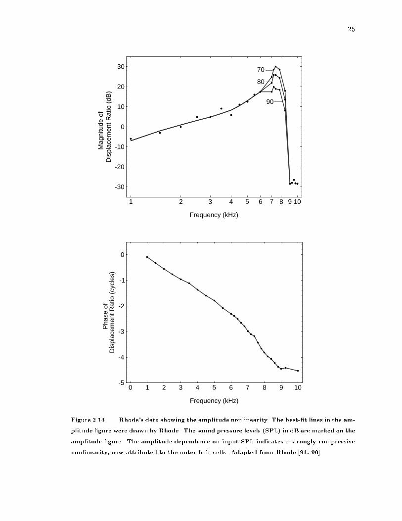
Rhode also measured frequency responses at di�erent input amplitudes, as shown in
Figure 2.13. These famous measurements illustrated the basilar membrane nonlinearity for

24
1
10
Frequency (kHz)
-30
-20
-10
0
10
20
30
Mag
nitu
de o
fD
ispl
acem
ent R
atio
(dB
)
x2 x1
0 1 2 3 4 5 6 7 8 9 10 11 12
Frequency (kHz)
-4
-3
-2
-1
0
Pha
se o
fD
ispl
acem
ent R
atio
(cy
cles
)
x2 x1
Figure 2.12 Rhode's data, taken from a live squirrel monkey using the M�ossbauer tech-
nique. The two curves indicate responses of the basilar membrane at two di�erent positions,
x1 and x2, on the basilar membrane, where x1 is 1.5 mm closer to the apex than x2. The best
�t lines in the amplitude �gure were drawn by Rhode. Adapted from Rhode [91].
25
1 2 3 4 5 6 7 8 9 10
Frequency (kHz)
-30
-20
-10
0
10
20
30
Mag
nitu
de o
fD
ispl
acem
ent R
atio
(dB
)
70
80
90
0 1 2 3 4 5 6 7 8 9 10
Frequency (kHz)
-5
-4
-3
-2
-1
0
Pha
se o
fD
ispl
acem
ent R
atio
(cy
cles
)
Figure 2.13 Rhode's data showing the amplitude nonlinearity. The best-�t lines in the am-
plitude �gure were drawn by Rhode. The sound pressure levels (SPL) in dB are marked on the
amplitude �gure. The amplitude dependence on input SPL indicates a strongly compressive
nonlinearity, now attributed to the outer hair cells. Adapted from Rhode [91, 90].

26
3 4 5 6 7 8 9 10
Frequency (kHz)
-10
0
10
20
30
Mag
nitu
de o
f Vel
ocity
(dB
) Minutes re Furosemide:-21+27+50
Figure 2.14 Ruggero and Rich's data, showing the e�ect of furosemide
on basilar-membrane response in the chinchilla. The three curves show the
normal membrane response (21 minutes before injection of furosemide), the
anesthetized response (27 minutes after injection), and the partially recovered
membrane response (50 minutes after injection). The frequency responses
were obtained by Fourier transformation of click responses at a 65 dB sound-
pressure-level. The experimental technique was laser Doppler velocimetry.
Phase measurements were not published. Adapted from Ruggero and Rich
[95].
the �rst time. If the basilar membrane vibrated linearly, all three curves would overlay one
another, since the transfer function is normalized for input level. The response of the system
is more peaked at lower input levels (70 dB) than at higher input levels (90 dB), illustrating
the compressive nonlinearity now ascribed to the outer hair cells. Rhode indicated a small
nonlinearity in the phase characteristic [90, p. 59].
Ruggero and Rich [95] have given compelling evidence that the amplitude nonlinearity
is due to mechanically active cells in the organ of Corti|very probably the outer hair cells.
By using the anesthetic furosemide to reduce the endocochlear potential, they e�ectively

27
2 4 6 8 10 20
Frequency (kHz)
10
20
30
40
50
60
70
80
Sou
nd P
ress
ure
Leve
l (dB
)
IsovelocityNeural Tuning Curve
Figure 2.15 A comparison of isovelocity response from a guinea-pig basilar
membrane and neural isoresponse from a guinea pig spiral ganglion cell. Both
curves show the level of input stimulation required to maintain a constant
output response. Adapted from Sellick, Patuzzi, and Johnstone [101].
robbed the organ of Corti of its supply of energy; they observed the dramatic change in the
basilar-membrane mechanical response shown in Figure 2.14.
In Figure 2.15, the isovelocity curve from a point on the guinea-pig cochlea is compared
to neural isoresponse curve from a spiral ganglion cell in the guinea pig. This famous
measurement, by Sellick, Patuzzi, and Johnstone [101], shows that the sharp tuning of an
auditory nerve �ber is determined at the mechanical level of the basilar-membrane vibration.
Since the system is nonlinear, these isoresponse tuning curves are not directly comparable
to transfer-function data, as pointed out by Lyon [63].
2.4 Abstraction
It is apparent that the cochlea is an extremely complex organ that exploits the physics
of wave propagation through a nonuniform medium, and exploits sophisticated neural ma-
chinery, to achieve its robust and sensitive encoding of auditory signals. We now turn to
the question of abstraction: which details are fundamentally required to capture essential
28
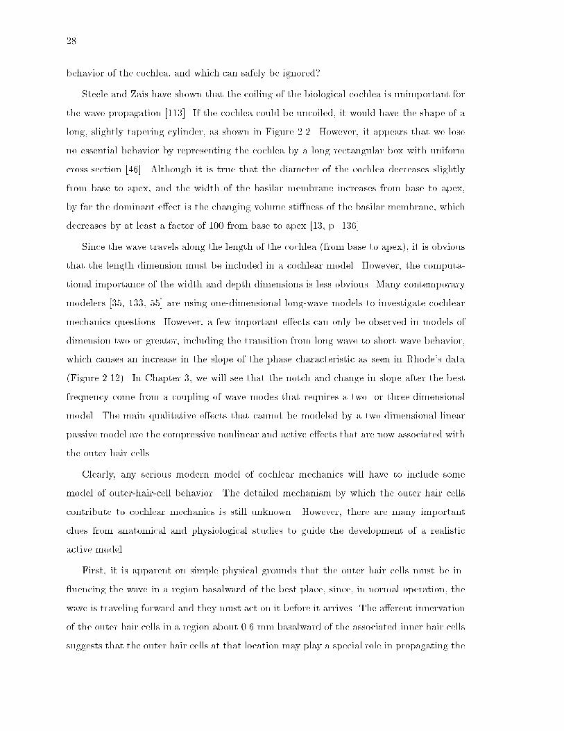
behavior of the cochlea, and which can safely be ignored?
Steele and Zais have shown that the coiling of the biological cochlea is unimportant for
the wave propagation [113]. If the cochlea could be uncoiled, it would have the shape of a
long, slightly tapering cylinder, as shown in Figure 2.2. However, it appears that we lose
no essential behavior by representing the cochlea by a long rectangular box with uniform
cross-section [46]. Although it is true that the diameter of the cochlea decreases slightly
from base to apex, and the width of the basilar membrane increases from base to apex,
by far the dominant e�ect is the changing volume sti�ness of the basilar membrane, which
decreases by at least a factor of 100 from base to apex [13, p. 136].
Since the wave travels along the length of the cochlea (from base to apex), it is obvious
that the length dimension must be included in a cochlear model. However, the computa-
tional importance of the width and depth dimensions is less obvious. Many contemporary
modelers [35, 133, 55] are using one-dimensional long-wave models to investigate cochlear
mechanics questions. However, a few important e�ects can only be observed in models of
dimension two or greater, including the transition from long-wave to short-wave behavior,
which causes an increase in the slope of the phase characteristic as seen in Rhode's data
(Figure 2.12). In Chapter 3, we will see that the notch and change in slope after the best
frequency come from a coupling of wave modes that requires a two- or three-dimensional
model. The main qualitative e�ects that cannot be modeled by a two-dimensional linear
passive model are the compressive nonlinear and active e�ects that are now associated with
the outer hair cells.
Clearly, any serious modern model of cochlear mechanics will have to include some
model of outer-hair-cell behavior. The detailed mechanism by which the outer hair cells
contribute to cochlear mechanics is still unknown. However, there are many important
clues from anatomical and physiological studies to guide the development of a realistic
active model.
First, it is apparent on simple physical grounds that the outer hair cells must be in-
uencing the wave in a region basalward of the best place, since, in normal operation, the
wave is traveling forward and they must act on it before it arrives. The a�erent innervation
of the outer hair cells in a region about 0.6 mm basalward of the associated inner hair cells
suggests that the outer hair cells at that location may play a special role in propagating the

29
Membrane Displacement
Fluid Pressure
Long-Wave Short-Wave Cut-Off
Outer Hair CellsDetection by
Inner Hair CellsConditioning by
Figure 2.16 Summary of the basic ideas in cochlear wave propagation. At
the basal end of the cochlea, waves travel with long wavelength and high speed.
As they travel, they slow down, and their wavelength decreases. In the short-
wave region, just before the amplitude of the membrane displacement peaks,
the outer hair cells in uence the signal, preferentially amplifying soft sounds
that would otherwise be too weak to hear. The membrane velocity is sensed
by the inner hair cells, is encoded as nerve impulses by the spiral ganglion
cells, and is transmitted to the brain via the cochlear nerve. Finally, the wave
dies out in the cut-o� region.
wave, and that there may be a functional advantage to monitoring their activity.
Rhode's evidence that the wave is in the short-wave region as it approaches the best
place [90] suggests that the outer hair cells only slightly basalward of the best place are
also in the short-wave region, or are in the transition between the long-wave and short-wave
regions. Recall that, in the long-wave region, the entire uid depth moves essentially as a
wall of uid, whereas in the short-wave region, only a small part of the total uid mass near
the membrane moves. So, we may speculate that it is more e�ective for the outer hair cells
to act on the wave in or near the short-wave region, since their forces will be acting on a
smaller e�ective uid mass.
All these considerations suggest the need for an active model, of at least dimension
two. Occam's razor suggests that we should favor a two-dimensional model over a three-
dimensional model, if there are no qualitative e�ects in the data or other evidence that
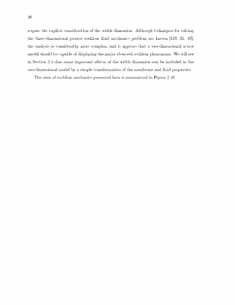
30
require the explicit consideration of the width dimension. Although techniques for solving
the three-dimensional passive cochlear uid mechanics problem are known [118, 21, 46],
the analysis is considerably more complex, and it appears that a two-dimensional active
model should be capable of displaying the major observed cochlear phenomena. We will see
in Section 3.4 that some important e�ects of the width dimension can be included in the
two-dimensional model by a simple transformation of the membrane and uid properties.
The view of cochlear mechanics presented here is summarized in Figure 2.16.

31
Chapter 3
Mathematical Models of Passive
Cochlear Mechanics
In Chapter 2, the anatomy and function of the cochlea were described in detail, and the
two-dimensional active model was justi�ed as the simplest model capable of exhibiting the
observed behavior of real cochleas. The passive two-dimensional model is the foundation
for the active two-dimensional model, so this chapter is devoted to describing the passive
two-dimensional model and relevant solution techniques. The Liouville{Green (LG) method
is emphasized, because it provides valuable insights into the problem.
Although the application of the LG method to cochlear mechanics problems has been
discussed in a great many papers, no analytical theory has been capable of explaining the
complete behavior of the traveling wave, including the plateau in the cut-o� region [112, 21].
Two innovations are described in this chapter. The �rst is a higher-order computation of
stapes displacement; this computation corrects a defect in the commonly accepted LG for-
mulation of the displacement ratio. The second is a new solution technique, called the
mode-coupling LG solution, in which energy is coupled into a second wave mode. The com-
bination of these two formulations leads to an analytical solution that agrees qualitatively
and quantitatively with numerical solutions, and, for the �rst time, o�ers an explanation
for the second vibration mode that was observed experimentally by Rhode in 1971 [91].
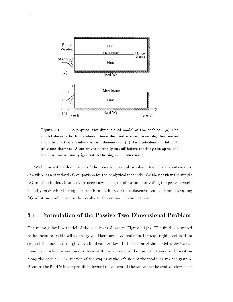
32
Membrane
Fluid
Fluid
Hard Wall
Helico-trema
(a)
(b) Hard Wall
Fluid
Membrane
x = 0 x = L
y = 0
y = h
y
x
Stapes
RoundWindow
Figure 3.1 The physical two-dimensional model of the cochlea. (a) The
model showing both chambers. Since the uid is incompressible, uid move-
ment in the two chambers is complementary. (b) An equivalent model with
only one chamber. Since waves normally cut o� before reaching the apex, the
helicotrema is usually ignored in the single-chamber model.
We begin with a description of the two-dimensional problem. Numerical solutions are
described as a standard of comparison for the analytical methods. We then review the simple
LG solution in detail, to provide necessary background for understanding the present work.
Finally, we develop the higher-order formula for stapes displacement and the mode-coupling
LG solution, and compare the results to the numerical simulations.
3.1 Formulation of the Passive Two-Dimensional Problem
The rectangular-box model of the cochlea is shown in Figure 3.1(a). The uid is assumed
to be incompressible with density �. There are hard walls on the top, right, and bottom
sides of the model, through which uid cannot ow. In the center of the model is the basilar
membrane, which is assumed to have sti�ness, mass, and damping that vary with position
along the cochlea. The motion of the stapes at the left side of the model drives the system.
Because the uid is incompressible, inward movement of the stapes at the oval window must

33
result in equal outward movement at the round window, so that movement of the uid in
the upper and lower chambers is in opposite directions, and pressure uctuations about the
resting pressure have opposite signs for corresponding points in the two chambers. Because
the solution is symmetrical in the two chambers, we may consider only one chamber, as
shown in Figure 3.1(b); however, we must account for the missing uid mass. Since waves
normally cut o� before reaching the apex, the helicotrema is usually ignored in the single-
chamber model. The length dimension of the model runs from x = 0 to x = L, and the
height dimension runs from y = 0 to y = h, as shown.
3.1.1 Hydrodynamics
The development of the hydrodynamics given in this section follows Lyon and Mead [67].
In general, the uid velocity vector v at any point (x; y) will have x and y components vx
and vy, respectively. It is convenient to de�ne a velocity potential �, such that
vx = �@�
@xand vy = �
@�
@y; (3:1)
or,
v = �r�:
For an incompressible uid, there is no net ow into or out of any small region, so
r � v =@vx
@x+@vy
@y= 0 or r2
� =@2�
@x2+@2�
@y2= 0: (3:2)
Thus, the velocity potential � obeys Laplace's equation.
The hard-wall boundary conditions at the right and bottom sides of the model imply
that there is no uid ow in a direction normal to the boundary. The boundary conditions
are thus
@�
@x= 0 at x = L;
and
@�
@y= 0 at y = 0: (3:3)
At x = 0, the motion of the uid is determined by the motion of the stapes, so the
34
boundary condition is
@�
@x= f(t) at x = 0: (3:4)
By considering a small element of uid and the forces acting on it, we can show that the
pressure p in the incompressible uid is related to the velocity of the uid v by the relations
�@p
@x= �
@vx
@tand �
@p
@y= �
@vy
@t; (3:5)
where � is the density of the uid. Substituting Equation 3.1 into Equation 3.5, we get the
relationship between the pressure and the velocity potential at any point in the uid:
p = �@�
@t; (3:6)
where p now represents the deviation from the pressure at rest.
3.1.2 Basilar-Membrane Boundary Condition
To complete the description of the problem, we must specify the boundary condition corre-
sponding to the basilar membrane. The displacement � of the membrane in the positive y
direction is related to the vertical uid velocity at y = h:
@�
@t= vy = �
@�
@y: (3:7)
Application of Newton's second law to an element of the membrane leads to the basilar-
membrane boundary condition [67]:
2�@�
@t= S(x)� + �(x)
@�
@t+M(x)
@2�
@t2at y = h; (3:8)
where S(x), �(x), and M(x) are the sti�ness, damping, and mass of the membrane, respec-
tively, all of which may vary as a function of position along the membrane. The sti�ness term
S(x)� has its form because the membrane acts like sti� uncoupled beams running across the
width of the membrane, as described in Chapter 2; hence, in the two-dimensional model,
the beams exert a restoring force that is only proportional to their displacement [120]. The
factor of 2 on the left side of the equation accounts for the complementary motion of the

35
r2� = 0
@�@y
= 0
@�@x
= 0@�@x
= f(t)
�2�@2�@t2
= S(x)@�@y
+ �(x) @2�
@y@t+M(x) @3�
@y@t2
y
xL00
h
Figure 3.2 The mathematical two-dimensional model of passive cochlear
mechanics. The contribution of the active outer hair cells is not included.
uid mass on the other side of the partition.
Some authors include a \tension" term, corresponding to longitudinal coupling between
the beamlike �laments of the basilar membrane. However, any signi�cant tension term
destroys the high-frequency cut-o� observed in real cochleas [67, 3, 60], and therefore most
authors neglect it.
Nearly all authors include membrane mass [137, 2, 78, 120, 112, 59, 22]; Lighthill
argues that membrane mass is necessary to account for the existence of a critical-layer-
absorption phenomenon, which is suggested by the sharp high-frequency cut-o� observed
in real cochleas. However, Lyon and Mead argue that the membrane mass can be neglected
if the wave energy is dissipated before the point of resonance [67]. In the present work, we
shall include the membrane mass as a free parameter.
Finally, there is the question of the active behavior of the outer hair cells, which a�ects
the partition boundary condition. A treatment of the active case is deferred until Chapter 5.
Di�erentiating both sides of Equation 3.8 with respect to t, and eliminating � via Equa-
tion 3.7, yields the basilar-membrane boundary condition:
� 2�@2�
@t2= S(x)
@�
@y+ �(x)
@2�
@y@t+M(x)
@3�
@y@t2at y = h: (3:9)
Figure 3.2 summarizes the two-dimensional boundary-value problem, corresponding to
the passive cochlear mechanics. It may be surprising that wave behavior is expected in
this problem, since the uid is incompressible; the wave behavior is made possible by the
coupled movement of the uid and membrane, rather than by compression of the uid itself.
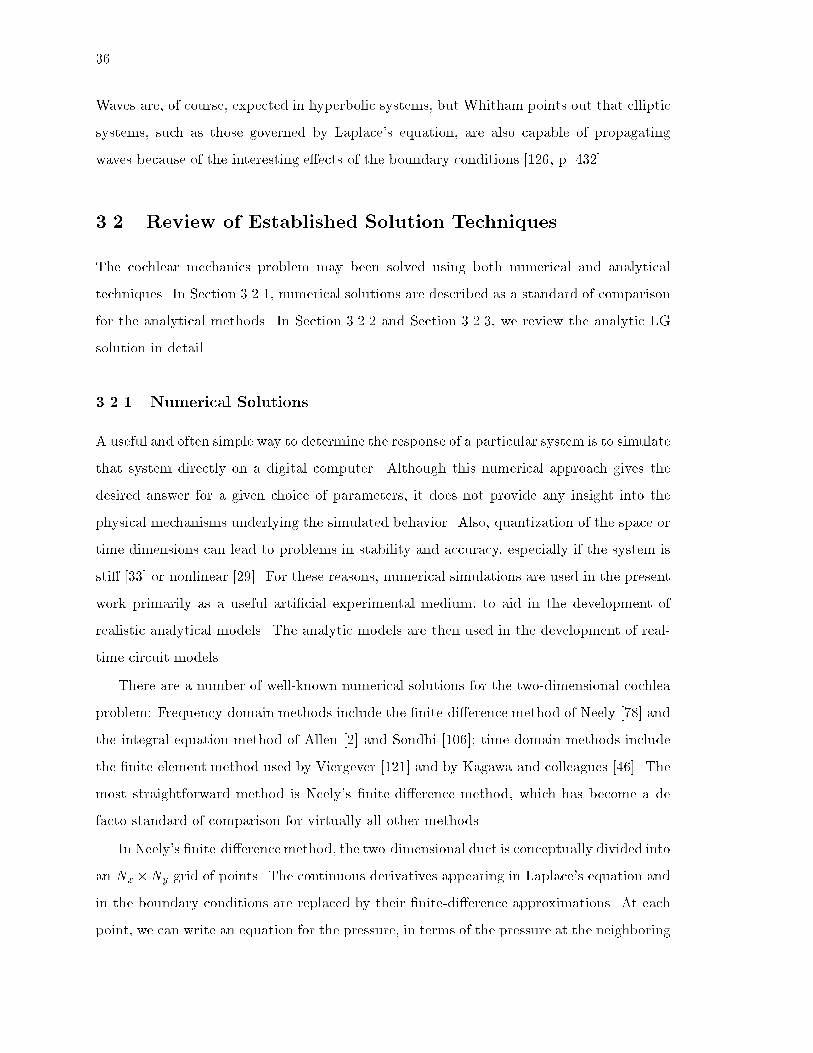
36
Waves are, of course, expected in hyperbolic systems, but Whitham points out that elliptic
systems, such as those governed by Laplace's equation, are also capable of propagating
waves because of the interesting e�ects of the boundary conditions [126, p. 432].
3.2 Review of Established Solution Techniques
The cochlear mechanics problem may been solved using both numerical and analytical
techniques. In Section 3.2.1, numerical solutions are described as a standard of comparison
for the analytical methods. In Section 3.2.2 and Section 3.2.3, we review the analytic LG
solution in detail.
3.2.1 Numerical Solutions
A useful and often simple way to determine the response of a particular system is to simulate
that system directly on a digital computer. Although this numerical approach gives the
desired answer for a given choice of parameters, it does not provide any insight into the
physical mechanisms underlying the simulated behavior. Also, quantization of the space or
time dimensions can lead to problems in stability and accuracy, especially if the system is
sti� [33] or nonlinear [29]. For these reasons, numerical simulations are used in the present
work primarily as a useful arti�cial experimental medium, to aid in the development of
realistic analytical models. The analytic models are then used in the development of real-
time circuit models.
There are a number of well-known numerical solutions for the two-dimensional cochlea
problem: Frequency-domain methods include the �nite-di�erence method of Neely [78] and
the integral-equation method of Allen [2] and Sondhi [106]; time-domain methods include
the �nite-element method used by Viergever [121] and by Kagawa and colleagues [46]. The
most straightforward method is Neely's �nite-di�erence method, which has become a de
facto standard of comparison for virtually all other methods.
In Neely's �nite-di�erence method, the two-dimensional duct is conceptually divided into
an Nx�Ny grid of points. The continuous derivatives appearing in Laplace's equation and
in the boundary conditions are replaced by their �nite-di�erence approximations. At each
point, we can write an equation for the pressure, in terms of the pressure at the neighboring

37
points. Additional terms appear in the equations for points located on the membrane
boundary or on the stapes wall. The problem reduces to the inversion of a sparse block-
tri-diagonal NxNy � NxNy matrix; this computation can be done very e�ciently [78, 86].
Equations and Mathematica code are given in Appendix A.
3.2.2 Exact Solution for a Uniform Cochlea
It is possible to determine an exact analytical solution for the passive two-dimensional
cochlea problem in which the properties of the membrane are constant. The solution of this
simple special case is a prerequisite for understanding the approximate LG solution for the
problem in which the membrane properties are allowed to change gradually.
It is convenient, but not necessary, to work with complex variables. We shall determine
a complex solution �(x; y; t) that satis�es the boundary-value problem, and then we shall
verify that the real part Re[�(x; y; t)] is also a solution.
We assume a solution of the form that we expect|that is, a wave traveling in the +x
direction with some (as yet unknown) y dependence:
�(x; y; t) = Y (y) exp i(!t� kx);
where k is the complex wavenumber and ! is the real frequency of the wave. Substituting
into Equation 3.2 yields
Y00(y) = k
2Y (y):
The solution of this equation that also satis�es the bottom boundary condition (Equation
3.3) is
Y (y) = B cosh(ky);
where B is a constant. Thus, the general solution that satis�es both Laplace's equation and
the bottom boundary condition is
�(x; y; t) = B cosh(ky) exp i(!t� kx): (3:10)
The membrane boundary condition provides the remaining constraint on the wave so-

38
lutions. To satisfy this boundary condition, we need the following derivatives:
@2�
@t2= �w2
�; (3.11)
@�
@y= kB sinh(ky) exp i(!t� kx) = k tanh(ky)�; (3.12)
@2�
@y@t= i!k tanh(ky)�; (3.13)
@3�
@y@t2= �!2k tanh(ky)�: (3.14)
Substituting these derivatives into the membrane boundary condition of Equation 3.9
yields the complex dispersion relation:
k tanh(kh) =2�!2
S + i�! �M!2: (3:15)
This important equation allows the wavenumber k to be determined when the physical
parameters (�, S, �, and M) and the input frequency ! are known. In general, the number
of solutions to the complex dispersion is in�nite. The solutions, or roots, must be found
numerically, since the equation is transcendental. It is also possible to make approximations
for the complex tanh function in certain regions, and to obtain closed-form approximate
solutions; these approximations are the mathematical basis for the long-wave, short-wave,
and cut-o� regions, and will be described shortly.
Interpreting the Solution
Complex variables were used in the derivation of the complex dispersion relation, the solu-
tion of which is a complex wavenumber k. However, we are interested only in the real part
of the velocity-potential solution.
Since the wavenumber k itself is complex, it will, in general, consist of a real part and
an imaginary part:
k = kr + iki;
where kr and ki are both real. The real part kr corresponds to an oscillatory waveform,
and the imaginary part ki corresponds to a wave that decays or grows as it travels.
We shall now check that the real part of the complex solution is also a solution. The

39
real part of the solution is
Re[�(x; y; t)] = Re[2A cosh(ky) exp i(!t� kx)]
= Re[2A cosh(fkr + ikigy) exp i(!t� fkr + ikigx)]
= Re[A exp(kry + ikiy + i!t� ikrx+ kix) +
exp(�kry � ikiy + i!t� ikrx+ kix)]
= A[exp(kry + kix) cos(!t� krx+ kiy) +
exp(�kry + kix) cos(!t� krx� kiy)]: (3.16)
We can substitute Equation 3.16 into Equations 3.2 and 3.3, to con�rm that the real solution
does indeed satisfy Laplace's equation and the bottom boundary condition. When we
substitute Equation 3.16 into the membrane boundary condition of Equation 3.9, we get
the following two real equations:
(S �M!2)(kr tanhkrh� ki tankih)� �!(ki tanhkrh+ kr tankih)� 2�!2 = 0;
and
(S�M!2)(ki tanh krh�kr tankih)��!(kr tanhkrh+ki tankih)�2�!
2 tanhkrh tan kih = 0;
which are simply the real and imaginary parts of the complex dispersion relation. So any
k that satis�es the dispersion relation can be substituted into Equation 3.10 to yield a
solution to the problem. Lyon and Mead emphasized the importance of working with the
real expression of Equation 3.16, but they were not able to verify that it was a solution in
the general case [67].
Following Lyon and Mead, the real solution of Equation 3.16 can be interpreted as a pair
of waves: One wave travels upward, with large amplitude near the partition, and deposits
energy into the partition (for ki < 0); the other wave travels away from the partition with
smaller amplitude. When k is purely real, the solution has the form of a simple traveling
wave in the +x direction, with a cosh(ky) y dependence. When k is purely imaginary,
the solution has the form of a decaying exponential in the +x direction, and looks like a

40
standing wave in the y direction.
In Chapter 2, the traveling wave was described as having three characteristic regions:
namely the long-wave, short-wave, and cut-o� regions. These important characterizations
are a direct result of the properties of the complex hyperbolic tangent function, which is
at the heart of the dispersion relation. As an aid to understanding and visualization, the
complex tanh function is plotted in Figure 3.3. The relationship between this important
function and the three traveling-wave regions is shown in Figure 3.4. We now describe the
long-wave, short-wave, and cut-o� approximations in detail.
Long-Wave Approximation
If the wavelength is long with respect to the height of the duct (jkhj � 1), the wave is
in the long-wave or shallow-water region. For jkhj � 1, we have tanh(kh) � kh, and the
complex dispersion relation reduces to
k �
s2�!2
h(S + i�! �M!2)for jkhj � 1: (3:17)
The condition jkhj � 1 is not very useful, since it does not indicate how small jkhj must
be to achieve a desired accuracy. If we are willing to accept a reasonable approximation
error|say 10 percent|we can use a more speci�c and less restrictive region of validity;
namely, we can use jkhj < :553.
Consider now the corresponding long-wave solution for the velocity potential. In the
long-wave region, we have
cosh(ky) � 1 for jkhj � 1 and 0 � y � h:
In this case, the amplitude of the velocity potential does not depend signi�cantly on the
vertical position, and the dominant uid motion is horizontal.
The long-wave condition generally arises at the beginning of the wave's journey along
the cochlea, where the sti�ness is very large and the damping and mass terms are relatively
small. In this case, the dispersion relation can be approximated as
k � !
r2�
hSfor jkhj � 1:

41
0
12
3
Re[kh]-6
-4
-2
0
Im[kh]
0
1
2
3
Re[Tanh[kh]]
0
12
3
Re[kh]-6
-4
-2
0
Im[kh]
0
1
2
3
0
12
3
Re[kh]-6
-4
-2
0
Im[kh]
-2
0
2
Im[Tanh[kh]]
0
12
3
Re[kh]-6
-4
-2
0
Im[kh]
-2
0
2
(a)
(b)
Figure 3.3 The complex function tanh(kh), as a function of its complex
argument kh. (a) The real part. (b) The imaginary part. Along the positive
real axis, the function behaves like the real tanh function. For jkhj � 1, the
function is essentially linear (i.e., tanh(kh) � kh). For Re[kh] � 1, the function
is essentially constant at tanh(kh) � 1. Along the negative imaginary axis, the
function appears like the tangent function, is periodic, and has singularities
near odd integer multiples of �i�=2.

42
Re[kh]
Im[kh]
1 2
�1
�2
00
��2
tanhkh � kh
Long-Wave
Re[kh] � 1
tanhkh � 1
Short-Wave
jkhj � 1
jkh + i�2j � 1
Cut-O�
tanhkh � 1
kh+i�=2
Figure 3.4 The relationship between the complex tanh function and the
three traveling-wave regions. A typical wavenumber trajectory is superim-
posed, for a �xed frequency and varying position x. For small x, waves begin
in the long-wave region. With increasing x, waves progress to the short-wave
region, and end in the cut-o� region. The transition from short-wave to cut-o�
is not straightforward; it is indicated by a broken line.

43
In this case, k and ! are linearly related, so the phase velocity c = !=k and the group
velocity U = @!=@k are equal:
c = U =
shS
2�;
and therefore the medium is not dispersive.
Short-Wave Approximation
If the wavelength is short with respect to the height of the duct (Re[kh] � 1), then the
wave is in the short-wave or deep-water region. For Re[kh] � 1, tanh(kh) � 1, and the
complex dispersion relation degenerates to the following simple form:
k �2�!2
S + i�! �M!2for Re[kh]� 1: (3:18)
Note that the wavenumber is independent of the duct height h in the short-wave case.
A more speci�c and less restrictive region of validity for the short-wave case, accurate to
within 10 percent, is Re[kh] > 1:522.
In the short-wave region, we have
cosh(ky) � exp(ky) for Re[kh]� 1 and 0 � y � h:
In this case, the uid motion decays exponentially with distance from the partition. In the
short-wave region, the wavenumber and frequency are not related linearly, and therefore
the wave is dispersive; that is, di�erent frequencies travel with di�erent velocities.
The conditions for the long-wave and short-wave cases are usually given as kh� 1 and
kh � 1, respectively [67]; however, these conditions are ambiguous when k is complex.
The unambiguous conditions given here|namely jkhj � 1 and Re[kh]� 1|are shown in
Figure 3.4 for the 10 percent accuracy conditions.
Cut-O� Approximation
Most of the wave energy is dissipated in the short-wave region. However, a small but
measurable amount of energy survives to the cut-o� region. Waves in the cut-o� region
are neither long nor short by the previous de�nitions; roughly speaking, they are vertical

44
standing waves, and are heavily damped in the +x direction. In this section, a novel
approximation for the cut-o� region is developed.
The condition for the wave to enter the cut-o� region is that the sti�ness and damping
terms in the complex dispersion relation (S and i�! respectively) have become small com-
pared to the mass term M!2. In this case, the dispersion relation can be approximated
as
k tanh(kh) � �2�
M:
For small values of the mass M , the right-hand side of the equation will take on a large
negative value. Familiarity with the complex tanh function indicates that the solutions will
appear near the values kh � �i�(n�1=2), where n is an integer|that is, the solutions will
appear near the singularities along the negative imaginary axis.
Since we are interested in the behavior near the singularities of the complex tanh func-
tion, a sensible approach is to take a Taylor expansion of the reciprocal of the complex tanh
function at the points of interest. Speci�cally, let
knh = �i�(n� 1=2) +� for n = 1; 2; 3; ::::
For �� 1, we have1
tanh knh� �;
and so the dispersion relation of Equation 3.15 reduces to
kn
�=
2�!2
S + i�! �M!2:
Solving for kn yields
kn =2i��!2(n� 1=2)
S + i�! � (M + 2�h)!2for n = 1; 2; 3; ::::
Modes with higher spatial frequency in the y dimension will die out exponentially faster
in the x dimension; therefore, it is reasonable, after some very small distance in x, to neglect

45
the higher modes, and to keep only the solution corresponding to n = 1:
k1 =i��!
2
S + i�! � (M + 2�h)!2:
In the far cut-o� region, where the sti�ness and damping terms have become negligible, the
expression reduces to
k1 = �i��
M + 2�h;
which, for small mass M , is a small perturbation around the point kh = �i�=2. If the
duct height h and uid density � are known, we can use this expression to estimate the
membrane mass M directly from biological data.
The region of validity of the cut-o� approximation for the �rst mode k1 is shown in
Figure 3.4. Note that there are in�nitely many singularities of the complex tanh function;
the �rst two are shown in Figure 3.3. Each singularity has a corresponding cut-o� mode,
but the �rst one is the most important, since it is the least heavily damped.
The question of multiple roots of the dispersion relation was raised by de Boer and
Viergever [21], in relation to the cut-o� behavior of the LG approximation. This point is
at the heart of the mode-coupling LG solution of Section 3.3.2.
No consideration has been given to the left and right boundary conditions at x = 0 and
x = L. Steele and Taber [112] point out that, at x = 0, one of the wavenumber solutions
corresponds to the traveling wave, whereas the others appear along the imaginary axis near
integer multiples of i�; these other solutions permit the stapes boundary condition to be
satis�ed exactly. These modes are clearly related to the cut-o� modes, in that they are
vertical standing waves that are attenuated heavily in the +x direction. Since these modes
have only a local e�ect near the stapes, they are usually ignored.
If we permit waves to reach the boundary at x = L, we should observe re ections.
However, in normal operation, membrane losses result in a sharp dissipation of the wave
energy at some position x < L, and therefore, the right-hand boundary condition is usually
ignored. The question of distributed re ections due to the changing medium was addressed
extensively by de Boer and colleagues, who concluded that forward-going waves are not
re ected to any signi�cant degree [19, 20], whereas backward-going waves are re ected
signi�cantly [18].

46
3.2.3 Approximate LG Solution for a Nonuniform Cochlea
We now turn to the case where the physical parameters of the cochlea are permitted to
change gradually. The general method of solution described here was �rst developed by
Liouville [61] and Green [40] in the mid-1800s to describe waves on shallow canals. The
Liouville{Green (LG) method is sometimes called the WKB or WKBJ method [112], after
Wentzel, Kramers, Brillouin, and Je�reys, who applied the technique in quantum mechanics
[70, 6] to determine connection formulae for linking oscillatory and exponential LG solutions
across a turning point on the real axis [121, p. 83]. The cochlear-mechanics problem is more
closely related to the original problem solved by Liouville and Green.
The following description of the LG method, as applied to cochlear mechanics, is based
on the work of Steele and Taber [112] and of de Boer and Viergever [21]. Their developments
are repeated here as background for the mode-coupling LG solution.
By combining Equations 3.10 and 3.7, we obtain the exact equation for basilar-membrane
displacement in the uniform medium:
�(x; t) =ik
!tanh(kh)�jy=h
=ikB
!sinh(kh) exp i(!t� kx)
= A exp i(!t� kx); (3.19)
where the amplitude factor A and wavenumber k do not depend on position x.
Any small section of the medium of length dx, over which the properties of the medium
change only slightly, behaves just as would a small section in a uniform medium|namely,
it contributes a phase shift krdx and a log gain kidx. The amplitude A must be adjusted to
conserve the ow of energy. The LG approximation amounts to writing Equation 3.19 as
�(x; t) = A(x) exp i(!t�
Z x
0
k(u)du); (3:20)
this equation clearly degenerates to Equation 3.19 when k is independent of x. Of course,
k will be determined by the dispersion relation of Equation 3.15, which, in the context of
the LG approximation, is often called the eikonal equation (from the Greek "��~!� [eikon]
meaning image).

47
To determine A(x), we shall exploit the fact that energy ows at the group velocity.
This point is discussed by Whitham [126] in a more general context, and is also valid for
dissipative systems [112]. Our approach will be (1) to �nd an expression for the energy ow
as a function of amplitude A, (2) to �nd an expression for the group velocity as a function of
k, and (3) to combine these expressions to determine A as a function of k. We shall develop
the condition for the undamped case, which is quite simple; the validity of the result in the
damped case has been shown by de Boer and Viergever [22]. An alternate approach, which
appeals to Hamilton's principle and Lagrangian mechanics, was used by Steele and Taber
[112], based on the general treatment by Whitham [126]. We now proceed with the simpler
�rst-principles energy approach.
The energy of the wave consists of three components: the kinetic energy of the membrane
mass Km, the potential energy of the membrane sti�ness Vm, and the kinetic energy of the
uid Kf . The time-averaged kinetic energy of the membrane mass per unit area is
Km =1
2�
Z 2�
0
1
2Mv
2yd� =
1
4M!
2A2: (3:21)
The time-averaged potential energy of the membrane sti�ness per unit area is
Vm =1
2�
Z2�
0
1
2S�
2d� =
1
4SA
2: (3:22)
To compute Kf , we need the velocity potential in terms of the amplitude factor A. Com-
bining Equations 3.7 and 3.19 yields
� = �i!A
k sinh(kh)cosh(ky) exp i(!t� kx):
The time-averaged kinetic energy of the uid per unit area is
Kf =
Z h
0
1
2�
Z2�
0
1
2(2�)(v2x + v
2y)d�dy (3.23)
=�!
2A2
2k tanh(kh)(3.24)
=1
2�!
2A2Q(k); (3.25)
where the 2� term accounts for the uid in both chambers, and the important function

48
Q(k) is de�ned as
Q(k) =1
k tanh(kh):
The energy balance then assumes the form
Vm = Kf +Km;
which is identical to the dispersion relation when Equations 3.21, 3.22, and 3.25 are substi-
tuted [22]. Finally, the total energy density E is given by
E = Vm +Kf +Km (3.26)
= 2Vm (3.27)
=1
2SA
2: (3.28)
We now have an expression for the energy density E as a function of membrane dis-
placement amplitude A. The second step in the derivation is to �nd an expression for the
group velocity U as a function of k. The lossless dispersion relation can be written in terms
of the function Q(k):
Q(k) =1
k tanh(kh)=S �M!
2
2�!2:
Di�erentiating with respect to k yields
@Q
@k=
@Q
@!
@!
@k(3.29)
= U@Q
@!; (3.30)
which leads to
U = �@Q
@k
�!
3
S
!: (3:31)
Energy ows at the group velocity [126]. For a constant rate of energy ow, we must
have
EU = const: (3:32)

49
Substituting Equations 3.28 and 3.31 into Equation 3.32 yields the simple result
A(k) = C
�@Q
@k
��1=2
=iCk tanhkhp
tanhkh+ khsech2kh;
where C is a constant of dimension (length)2. This important equation is called the transport
equation, since it relates to the transport of energy.
Substituting this result into Equation 3.20 yields the full equation for the membrane
displacement:
�(x; t) =iCk tanhkhp
tanhkh+ khsech2khexp i(!t�
Z x
0
k(u)du); (3:33)
where k is the local root of the dispersion relation. Combining this result with Equation
3.7 yields the expression for the velocity potential:
�(x; y; t) =C! cosh(ky)
cosh(kh)ptanhkh+ khsech2kh
exp i(!t�Z x
0
k(u)du); (3:34)
We can derive similar expressions for the membrane velocity vy(x; t), and uid pressure
p(x; y; t), using the de�ning relations 3.1 and 3.6.
Rhode's data are expressed in the form of a ratio of basilar-membrane displacement to
malleus displacement, which we assume is proportional to stapes displacement [91]. We
must now compute the stapes displacement.
Recall that the horizontal uid velocity vx(x; y) at any point (x; y) in the uid is
vx(x; y) = �@�
@x:
The horizontal uid displacement dx(x; y) is the time integral of the horizontal uid velocity.
For a sinusoidal disturbance with angular frequency !, we have
dx(x; y) =i
!
@�
@x: (3:35)

50
Di�erentiating Equation 3.34 with respect to x yields
@�
@x= (�ik+ O[k0(x)])�(x; y): (3:36)
As a �rst approximation, we shall ignore the terms involving k0(x). Combining Equations
3.36 and 3.35 yields
dx(x; y) =k
!�(x; y): (3:37)
Following Steele and Taber [112], the stapes displacement dst is the value of the hori-
zontal uid displacement at x = 0, averaged over the height of the duct h:
dst =1
h
Z h
0
dx(0; y)dy (3.38)
=k0
!h
Z h
0
�(0; y)dy;
where k0 is the value of the wavenumber k evaluated at x = 0. Substituting Equation 3.34
and performing the integration yields
dst =C tanh(k0h) exp(i!t)
h
qtanh(k0h) + k0hsech
2(k0h): (3:39)
Combining Equations 3.33 and 3.39 yields the ratio D of membrane to stapes displace-
ment:
D(x; !) =�
dst= ikh
tanh(kh)
tanh(k0h)
stanh(k0h) + k0hsech
2(k0h)
tanh(kh) + khsech2(kh)exp�i
Z x
0
k(u)du: (3:40)
Note that the above expression is only a �rst approximation, since the terms involving k0(x)
in dst have been neglected.
The general LG solution for the velocity potential given in Equation 3.34 degenerates
to the following simple form at y = h under the long-wave approximation:
�(x; t) = const k�1=2 exp i(!t�
Z x
0
k(u)du); (3:41)
where k is given by the simple long-wave expression of Equation 3.17. This form was �rst
applied to cochlear mechanics problems by Zweig, Lipes, and Pierce [134]. The validity

51
criterion for the one-dimensional long-wave LG approximation is [70, 121]
���� 1k2
dk
dx
����� 1:
Zweig and colleages also showed that it is possible to evaluate the integral in closed form,
under the scaling assumption:
S(x) = S0 exp(�2x=d);
�(x) = �0 exp(�x=d);
M(x) = const:
Alternate derivations of the long-wave LG result are given by Lighthill [60, p. 189{90] and
by Viergever [121, p. 103{106].
In the short-wave region, the general LG solution for the velocity potential given in
Equation 3.34 degenerates to the following simple form at y = h:
�(x; t) = const exp i(!t�
Z x
0
k(u)du);
where k is given by the simple short-wave expression of Equation 3.18. This form was
�rst applied to cochlear mechanics problems by Siebert [103]. Under the same scaling
assumptions used by Zweig, Lipes and Pierce, for the long-wave case, we can evaluate the
short-wave integral in closed form.
A Mathematica implementation of the two-dimensional LG algorithm is given in Ap-
pendix A.
Comparison of LG and Finite-Di�erence Results
Steele and Taber compared their LG results to the �nite-di�erence results of Neely for
a number of di�erent frequencies, using identical parameters for the two models [112].
Their results have been recomputed, and are presented here for comparison with the mode-
coupling LG solution presented in section 3.2. The physical parameters used for their
comparison were

52
S(x) = 1:0� 107 e�x=d g s�2 mm�2;
�(x) = 2 g s�1 mm�2;
M = 1:5� 10�3 g mm�2;
d = 5 mm;
h = 1 mm;
L = 35 mm;
� = 1:0� 10�3 g mm�3:
Note that neither Neely nor Steele and Taber regarded these parameters as physically
realistic. In particular, the membrane mass M is unrealistically large.
The amplitude and phase of the basilar-membrane displacement ratios are shown in
Figure 3.5 for the two methods. Clearly, the LG solution captures the general behavior of
a gentle increase in amplitude toward a peak, followed by a sharp cut-o�. However, the
quantitative agreement is poor for the lowest frequencies, and in the cut-o� region, the
amplitude of the LG solution decreases much too fast, and the phase behavior is incorrect.
Both of these problems are addressed in Section 3.3.
3.3 New Solution Techniques
The LG solution is based on sound physical reasoning about the cochlear-mechanics prob-
lem. For that reason, the failure of the LG solution to agree with numerical solutions in the
cut-o� region is mysterious [112, 121, 21]. The poor agreement between the LG solution
and numerical solutions at low frequencies has generally been attributed to an inherent
limitation of the LG method. Both of these discrepancies are remedied in this section.
3.3.1 Higher-Order Calculation of Stapes Displacement
To reconcile the numerical and LG solutions, we �rst consider the problem of poor match at
low frequencies, as shown in Figure 3.5. Recall that, in the derivation of stapes displacement
(Equation 3.39), terms involving k0(x) were dropped as a �rst approximation. However,
these terms are dominant when the wavelength near the stapes is very long, and they
should not be neglected.

53
0 5 10 15 20 25 30 35
Distance from stapes (mm)
-80
-60
-40
-20
0
20
Mag
nitu
de o
fD
ispl
acem
ent R
atio
(dB
)
0.40.81.63.26.4 kHz
0 5 10 15 20 25 30 35
Distance from stapes (mm)
-3
-2
-1
0
Pha
se o
fD
ispl
acem
ent R
atio
(cy
cles
)
0.4
0.81.63.26.4kHz
(a)
(b)
Figure 3.5 Comparison of LG and �nite-di�erence solutions for the basilar-
membrane displacement ratio, for various frequencies. (a) Magnitude. (b)
Phase. The �nite-di�erence solutions are shown as solid lines; the LG solutions
are shown as dashed lines. The solutions were recomputed from Steele and
Taber [112] and Neely [78]. Small errors by Steele and Taber were corrected in
a subsequent paper by Steele and Miller [110]. Input frequencies are marked
in kHz. The agreement is progressively worse for low frequencies, and there is
sharp divergence between the numerical solutions and the LG solutions after
the peak.

54
The complete expression for @�=@x is
@�
@x=
��ik �
2k0h(1� kh tanhkh)
2kh+ sinh2kh+ k
0(y tanhky � h tanhkh)
��(x; y): (3:42)
Note that this expression is consistent with Equation 3.36.
Combining Equations 3.42, 3.35, 3.38, and 3.34, and performing the integration, yields
the complete expression for the stapes displacement:
dst =CT (k0; k
00) exp(i!t)
h
qtanh(k0h) + k0hsech
2(k0h); (3:43)
where
T (k0; k0
0) = tanh(k0h)
�1�
ik00
k20
�2ik00h(1� k0h tanh(k0h))
k0[2k0h+ sinh(2k0h)]�
ik00h tanh(k0h)
k0
�+ik00h
k0;
and k00 is the value of k0(x) evaluated at x = 0. Equation 3.43 degenerates to Equation 3.39
if terms involving k00 are neglected.
Combining Equations 3.33 and 3.43 yields the complete expression for D, the ratio of
membrane to stapes displacement:
D(x; !) =�
dst= ikh
tanh(kh)
T (k0; k00)
stanh(k0h) + k0hsech
2(k0h)
tanh(kh) + khsech2(kh)exp�i
Z x
0
k(u)du: (3:44)
Equation 3.44 degenerates to Equation 3.40 when the terms involving k00 are neglected.
Since k(x) must be determined numerically, we might be tempted to use a �nite-
di�erence approximation to determine k0(x). However, a more elegant and accurate method
is available. Recall that k is the solution of the dispersion relation
k tanh(kh) = S(x);
where
S(x) =2�!2
S + i�! �M!2: (3:45)

55
Di�erentiating with respect to x yields
k0 tanh(kh) + k[k0hf1� tanh2(kh)g] = S 0:
Rearranging leads to a convenient expression for k0(x):
k0 =
S 0
kh+ tanh(kh)� kh tanh2(kh):
S 0(x) is easy to �nd, since the physical parameters on which S(x) depends are usually
assumed to have exponential dependence on x.
The improved calculation of stapes displacement has been included in the LG calcula-
tion, and the results are plotted in Figure 3.6. The agreement with the numerical solution
is improved over the �rst-order approximation in Figure 3.5.
3.3.2 The Mode-Coupling LG Solution
We now consider the remaining disagreement between the LG and numerical solutions in
the cut-o� region, after the best place. The reason for the disagreement is that the LG
solution fails to satisfy Laplace's equation in the uid just prior to the cut-o� region.
Background: Limited Validity of the LG Solution
In this section, we shall see that the LG solution associated with the primary root k(x) fails
to satisfy Laplace's equation in the uid just basalward of the cut-o� region.
Recall that the LG solution for the velocity potential (Equation 3.34) is
�(x; y; t) = C!a(x)cosh(ky)
cosh(kh)exp i(!t�
Z x
0
k(u)du);
where
a(x) =1p
tanh kh+ khsech2kh;
and, of course, k = k(x). This approximate solution for � was designed to satisfy Laplace's
equation|that is, to ensure that the ow into any region of space in the x direction @2�=@x2
is exactly canceled by the ow out of that region in the y direction @2�=@y2. Since the LG
solution is only approximate, we do not expect that r2� is exactly zero; we expect only

56
0 5 10 15 20 25 30 35
Distance from stapes (mm)
-80
-60
-40
-20
0
20
M
agni
tude
of
Dis
plac
emen
t Rat
io (
dB)
0.40.81.63.26.4 kHz
0 5 10 15 20 25 30 35
Distance from stapes (mm)
-3
-2
-1
0
Pha
se o
fD
ispl
acem
ent R
atio
(cy
cles
)
0.4
0.81.63.26.4kHz
(a)
(b)
Figure 3.6 LG solution with improved calculation of stapes displacement
(dashed lines) compared with �nite-di�erence solution (solid lines), using
Neely's parameters. (a) Magnitude. (b) Phase. Input frequencies are marked
in kHz.

57
that the net accumulation or loss in the region is small compared to the amount owing
through it, for a small relative error. Since @2�=@y2 = k2�, a reasonable criterion for the
solution to be valid is
jr2�j � jk2�j or
�����r2�
k2�
������ 1: (3:46)
We shall refer to the term jr2�
k2�j as the Relative Laplace Error, or RLE. A nonzero value
of RLE implies that the assumption of uid incompressibility is being violated.
The Laplacian of the velocity potential is
r2�(x; y; t) � �i
�k0 +
2a0k
a+ 2kk0(h tanhkh� y tanhky)
��(x; y; t);
where the terms involving higher-order derivatives a00(x), k00(x), and a0(x)k0(x) have been
dropped. Evaluating a0(x) in terms of k(x) and k
0(x), the validity condition of Equation
3.46 becomes
���� k0k2
�1�
4kh(1� kh tanhkh)
2kh+ sinh2kh+ 2k(y tanhky � h tanhkh)
������ 1: (3:47)
de Boer and Viergever [21] give the validity condition of the two-dimensional model as
���� k0k2
����� 1
which is equivalent to Equation 3.47 at y = h when the term corresponding to 2a0k=a is
neglected.
It is instructive to consider a particular example. Let us arbitrarily use Neely's param-
eters with an input frequency of f = 2:26 kHz. In Figure 3.7(a), jr2�=k
2�j is plotted at
the membrane (y = h) and at the bottom of the duct (y = 0). The LG solution at the
membrane suddenly fails to satisfy Laplace's equation at about x = 17:4 mm, at approxi-
mately the place where the LG solution and the numerical solution diverge (see Figure 3.5).
Interestingly, the solution begins to fail at the bottom of the duct at about x = 15 mm, over
2 mm before the failure is observed at the membrane. In Figure 3.7(b), the RLE is shown
as a density plot as a function of position in the duct. Clearly, the sudden divergence at the
membrane is actually the culmination of a gradual process that grows over a considerable

58
0 5 10 15 20 25
Distance from Stapes (mm)
0
1
2
3
4
RLE
at y
=0
0 5 10 15 20 25
Distance from Stapes (mm)
0
0.2
0.4
0.6
0.8
1
RLE
at y
=h
0 1 2 3 4 5 6 7 8 9 10 11 12 13 14 15 16 17 18 19 20 21 22 23 24 25
Distance from stapes (mm)
00.20.40.60.8
1.
Hei
ght (
mm
)
(a) (b)
(c)
Figure 3.7 Validity of LG solution, for Neely's parameters with f = 2.26
kHz. (a) Relative Laplace Error (RLE) at y=h. (b) RLE at y=0. Note the
di�erent scales between (a) and (b); the error begins at smaller x values and
becomes larger at y=0 than at y=h. (c) RLE plotted as density plot. White
corresponds to RLE=0; black corresponds to RLE � 1.

59
0 1 2 3 4 5 6 7 8 9 10 1112 13 14 15 16 17 18 19 20 2122 23 24 25
Distance from stapes (mm)
00.20.40.60.8
1.
Hei
ght (
mm
)
0 1 2 3 4 5 6 7 8 9 10 1112 13 14 15 16 17 18 19 20 2122 23 24 25
Distance from stapes (mm)
00.20.40.60.8
1.
Hei
ght (
mm
)
(a)
(b)
Figure 3.8 Phase of uid pressure in (a) the �nite-di�erence solution, and
(b) the LG solution, using Neely's parameters with f=2.26 kHz. The numerical
solution shows a forward-going traveling wave, and a standing wave after the
best place. The LG solution also shows a forward-going traveling wave; in
addition, the LG solution has a multinodal standing-wave pattern after the
best place, and has a small region at the bottom of the duct at about x=17
mm, where there is a backward-going wave.
distance in the uid, and that begins at the bottom of the duct.
Further evidence for the failure of the classic LG solution lies in the phase characteristic.
In Figure 3.8, the phase of the uid pressure throughout the duct is compared for the
numerical solution and for the LG solution. The numerical solution shows a traveling wave
that \lifts o�" the bottom of the duct, leaving a standing-wave pattern after the best place.
The LG solution also shows the traveling wave, but ends in a di�erent multinodal standing-
wave pattern. On closer inspection, we see a small triangular region near the bottom of
the duct, near x = 17 mm, where the wave is traveling backward, as though from a small
source on the bottom wall. This nonphysical behavior is occurring in the region of high
RLE shown in Figure 3.7. The high RLE and the backward-going wave are the result of
the breakdown of the assumption that the wavenumber varies slowly|an assumption that
lies at the heart of the LG approximation.

60
Recall that the wavenumber is the solution of the dispersion relation, and, in fact, there
are in�nitely many solutions. So far, we have been concerned only with the wavenumber that
corresponds to the traveling-wave solution, and we have ignored the more heavily damped
modes. However, to understand how to repair the LG solution, we must now consider the
other wavenumber solutions. The �rst few wavenumber solutions are shown in Figure 3.9,
for Neely's parameters at 400 Hz, 800 Hz, and 1131 Hz.
The simplest case is shown in Figure 3.9(a) at 400 Hz, where the wavenumber trajectories
for the various modes are completely independent. This �gure is directly comparable to
Figure 3.4. The primary traveling-wave mode begins near the origin in the long-wave region,
arcs around toward the short-wave region, and ends in the cut-o� region near �i�=2. The
other modes begin near integer multiples of �i�, and follow similar clockwise paths.
In Figure 3.9(b), at 800 Hz, the traveling-wave solution interacts with the solution that
originates at �i�. This nontraveling-wave solution plays a special role in the cut-o� region,
as we shall see shortly. In recognition of its special signi�cance, we shall call it the cut-o�
mode; it is shown as a dashed line in Figure 3.9. Initially, the traveling-wave solution and
the cut-o� solution follow paths like the ones shown in part (a), but then the traveling
wavenumber solution arcs around the cut-o� solution, ending near �i�; the cut-o� solution
follows an upward path and ends near �i�=2. The other modes are not a�ected.
In Figure 3.9(c), at 1131 Hz, the traveling-wave solution interacts with the wavenumber
solutions beginning at �i� and �2i�, enclosing them and forcing them to follow upward
paths. This pattern continues at higher frequencies for Neely's choice of parameters; the
traveling-wave solution can encircle many of the other solutions. For Neely's parameters,
with an an input frequency of 9051 Hz, the traveling-wave solution ends near �i18�, en-
circling 18 other solutions. In all cases, the mode that ends near �i�=2 is either the
traveling-wave mode, as in part (a), or the cut-o� mode, as in parts (b) and (c), which
begins near �i�.
Recall that the imaginary part of a wavenumber ki determines the degree of damping
of the corresponding wave. In part (a), the cut-o� mode is always damped more heavily
than is the traveling-wave mode, so any energy in the cut-o� mode will always die out in
a short distance. In part (b), the cut-o� mode begins with heavier damping than does
the traveling-wave mode, but ends with lighter damping. The cause of the disagreement

61
1 2 3 40
−π
−2π
−3π
1 2 3 40
−π
−2π
−3π
1 2 3 40
−π
−2π
−3π
Re[kh]
Im[kh]
(a) f=400 Hz (c) f=1131 Hz(b) f=800 Hz
Figure 3.9 Example wavenumber trajectories at three di�erent frequencies,
using Neely's parameters. The traveling wavenumber trajectory is shown as
a solid line; the cut-o� wavenumber trajectory is shown as a dashed line; the
other wavenumber trajectories are shown as gray lines. These trajectories may
be compared to the typical wavenumber trajectory in Figure 3.4. In all cases,
the traveling-wave trajectory begins near the origin for small position x, and
follows a clockwise path with increasing x.

62
between the numerical solution and the LG solution in Figure 3.5 is now evident. By some
mechanism, energy is being transferred into the cut-o� mode. After the best place, the
cut-o� mode is less heavily damped than the traveling-wave mode, and so its more gentle
decay dominates in the cut-o� region.
Viergever [121] observed that the moderate slope in the cut-o� region was consistent with
the lightly damped cut-o� mode. He also observed that the bend in the amplitude curve
appeared near the resonance point, so he proposed splicing together the traveling-wave and
cut-o� solutions at the resonance point, prescribing continuity of basilar membrane velocity
at the splice. Viergever's result showed a qualitatively correct behavior, but the amplitude
response was incorrect by a constant factor and the phase showed a constant di�erence with
the correct one. When the locus of the discontinuity was shifted appropriately, both defects
were reduced. de Boer and Viergever observed that [21, p. 146] \the assumptions invoked
in this procedure seem not well justi�ed but the gain is considerable: in the cut-o� region
the LG [WKB] response behaves in the correct way. Up to now the optimum criterion for
this procedure has not been found so we must leave the situation as it is."
It is clear that some deeper physical justi�cation is needed to explain the appearance of
energy in the cut-o� mode. The key to solving the problem is the failure of the traveling-
wave mode to satisfy Laplace's equation in the region just prior to the best place. In that
region, the wavenumber is changing so fast that the simple LG solution breaks down, and
additional degrees of freedom are required to allow Laplace's equation and all the boundary
conditions to be satis�ed.
Development of the Mode-Coupling LG Solution
We now propose the following form of the velocity-potential solution:
�(x; y; t) = �1(x; y; t) + c(x)�2(x; y; t); (3:48)
where �1 is the traveling-wave solution with wavenumber k1, which originates near k1 � 0
for x = 0; �2 is the cut-o� solution with wavenumber k2, which originates near k2 � �i�
for x = 0; and c(x) is the coupling coe�cient. �1 and �2 have been determined already
from Equation 3.34 and from the dispersion relation of Equation 3.15; we must �nd c(x)

63
such that the composite solution � satis�es Laplace's equation.
For Laplace's equation to hold, we must have
r2� = r2
�1 + cr2�2 + 2
@c
@x
@�2
@x+
@2c
@x2�2 = 0:
This equation implies that c = c(x; y) to make r2�(x; y) vanish at every point. However,
a good approximate solution is possible with c = c(x) alone, so let us specify that the total
error must vanish in a vertical slice:
Z h
0
r2� dy =
Z h
0
r2�1 dy + c(x)
Z h
0
r2�2 dy + 2c0(x)
Z h
0
@�2
@xdy + c
00(x)
Z h
0
�2 dy = 0:
This equation has the form
c00(x) + P (x)c0(x) +Q(x)c(x) = R(x); (3:49)
that is, it is a second-order ordinary di�erential equation in c(x), with nonconstant coe�-
cients given by
P (x) =2R h0
@�2@x
dyR h0�2 dy
; (3.50)
Q(x) =
R h0r2
�2 dyR h0�2 dy
; (3.51)
R(x) = �
R h0r2
�1 dyR h0�2 dy
: (3.52)
It is possible to obtain approximate closed-form expressions for the preceding integrals;
the lengthy formulae are given in Appendix A. Typical behavior of the functions P (x), Q(x)
and R(x) is shown in Figure 3.10.
Solving for the Coupling Coe�cient c(x)
There are in�nitely many solutions to the general second-order di�erential equation [104].
We must specify two additional boundary conditions to obtain a particular solution. At the
left-hand boundary (x = 0), we expect that � = �1 should be a good solution, as con�rmed
in Figure 3.5, and as evidenced by the small RLE in Figure 3.7. Thus, at the left-hand

64
0 5 10 15 20 25
Distance from stapes (mm)
-100
0
100
200
300
400
Mag
nitu
de (
dB)
R(x)
P(x)
Q(x)
Figure 3.10 Magnitude of P(x), Q(x) and R(x) in dB, for Neely's param-
eters at f=2.26 kHz. Note that 20 dB corresponds to a factor of 10, so R(x)
increases by a factor of 1023 between x=0 and x=16.5 mm.

65
boundary, there is no need for �2, so the boundary condition is
c(x) = 0 at x = 0: (3:53)
At x = L, R(x) and Q(x) are small compared to P (x), which is near unity, as shown in
Figure 3.10. So Equation 3.49 has the form
c00(x) + c
0(x) � 0; (3:54)
that is, all derivatives of c(x) are nearly 0. Thus, the required right-hand boundary condition
is
c0(x) = 0 at x = L: (3:55)
The di�erential Equation 3.49, and the two boundary conditions of Equations 3.53 and
3.55, constitute a one-dimensional boundary-value problem with nonconstant coe�cients,
for which there is no general closed-form solution [104]. We can solve the problem numeri-
cally by dividing the space dimension into small increments, by writing the �nite-di�erence
approximations to the spatial derivatives, and by solving the resulting tridiagonal matrix.
The procedure is given in detail in Appendix A.
Performance of the Mode-Coupling LG Solution
Examples of the amplitude and phase of the membrane displacement ratios are shown in
Figure 3.11 for the mode-coupling LG and �nite-di�erence methods. Clearly, the mode-
coupling LG method has predicted the correct amount of energy to couple into the k2
solution, to give good agreement with the numerical solution. The corresponding coupling
coe�cients c(x) are shown in Figure 3.12. Although the coupling coe�cients are increasing
at a great rate, they are primarily balancing the natural decay of the cut-o� mode, resulting
in a gradual increase of the contribution of the cut-o� mode up to the best place, as shown
in Figure 3.13. Note that the cut-o� mode has its maximum amplitude in the vicinity of
the best place. Beyond the best place, the traveling-wave mode decays quickly, whereas the
cut-o� mode decays less quickly. Let us call the location at which the amplitudes of the
two modes are equal the crossover point.

66
0 5 10 15 20 25 30 35
Distance from stapes (mm)
-80
-60
-40
-20
0
20
M
agni
tude
of
Dis
plac
emen
t Rat
io (
dB)
0.40.81.63.26.4 kHz
0 5 10 15 20 25 30 35
Distance from stapes (mm)
-3
-2
-1
0
Pha
se o
fD
ispl
acem
ent R
atio
(cy
cles
)
0.4
0.81.63.26.4kHz
(b)
(a)
Figure 3.11 Comparison of mode-coupling LG and �nite-di�erence solu-
tions for the basilar-membrane displacement ratio, for various frequencies. (a)
Magnitude. (b) Phase. The �nite-di�erence solutions are shown as solid lines;
the mode-coupling LG solutions are shown as dashed lines. Input frequencies
are marked in kHz.

67
0 5 10 15 20 25 30 35
Distance from stapes (mm)
0
200
400
600
800
Mag
nitu
de o
f c(x
) (d
B)
0.4
0.8
1.6
3.2
6.4 kHz
Figure 3.12 Magnitude of coupling coe�cients c(x) in dB for Neely's pa-
rameters. Input frequencies are shown in kHz.

68
0 5 10 15 20 25 30
Distance from stapes (mm)
-80
-60
-40
-20
0
20
Mag
nitu
de o
fD
ispl
acem
ent R
atio
(dB
)
composite
traveling wave
cut-off
Figure 3.13 Contribution of traveling-wave and cut-o� modes to the com-
posite displacement ratio, for Neely's parameters at f=2.26 kHz. From x=0
to x=17.4 mm, the traveling-wave mode dominates. Beyond x=17.4 mm, the
cut-o� mode dominates. The location at which the amplitudes of the two
modes are equal is called the crossover point.

69
0 2 4 6 8 10 12 14
Distance from stapes (mm)
-80
-60
-40
-20
0
20
Mag
nitu
de o
fD
ispl
acem
ent R
atio
(dB
)
0 2 4 6 8 10 12 14
Distance from stapes (mm)
-3
-2
-1
0
Pha
se o
fD
ispl
acem
ent R
atio
(cy
cles
)
Composite
Traveling-Wave
Cut-Off
(a)
(b)
Figure 3.14 Explanation of the notch. (a) The notch in the amplitude
response at the crossover point is caused by destructive interference of the
traveling-wave and cut-o� modes. (b) At the crossover point (x � 10.4 mm),
the two wave modes have a relative phase di�erence of about 3.5 cycles. Neely's
parameters were used, at f=4.53 kHz.

70
15
16
17
18
19
x (mm)
00.2
0.40.60.81.
y (mm)
4060
80
100
|P| (dB)
15
16
17
18
19
x (mm)
00.2
0.40.60.81.
y
4060
80
10
Figure 3.15 The notch in the pressure pro�le, for Neely's parameters, with
f=2.26 kHz. Although destructive interference of the traveling-wave and cut-
o� modes is not evident in the displacement-ratio solution of Figure 3.11, it is
clearly evident in the uid-pressure solution. Destructive interference in the
uid depth causes the \hole" in the uid-pressure pro�le near x=17 mm and
y=0.6 mm.

71
The \notch" often observed in the amplitude of the displacement ratio at the crossover
point (see Figure 2.12) has never been explained satisfactorily. de Boer and Viergever
postulated that it may be the result of a \re ection on a micro-scale" due to the extremely
rapid change of wavenumber near the resonance region [21, p. 146]. However, the mode-
coupling LG solution o�ers a simple and physically sound explanation, based on destructive
interference of the traveling-wave and cut-o� modes. In the vicinity of the crossover point,
the two wave modes have comparable amplitude. Their relative phases determine whether
the two modes interfere constructively, as in Figure 3.13, or destructively, as in Figure 3.14.
The phases of the traveling-wave and cut-o� modes are shown in Figure 3.14(b) for the
destructive interference case. At the crossover point (x � 10:4 mm), there is a phase
di�erence of about 3.5 cycles between the two displacement-ratio solutions, so the sum of
the two solutions shows a substantial cancellation, causing the notch in the magnitude curve.
The appearance of the notch requires a nearly exact antiphase relationship between the two
displacement-ratio solutions at the crossover point, so the notch is not always observed.
However, destructive interference usually occurs at some depth in the uid pressure, as
shown in Figure 3.15. Note that this strangely localized cancellation is not an \eddy,"
which could arise only in a nonlinear three-dimensional model [41, p. 5].
A legitimate concern is whether the coupling of energy into the cut-o� mode is an artifact
of the simpli�ed two-dimensional model, or whether it corresponds to a real behavior in the
biological cochlea. Rhode was the �rst to observe the notch and change in slope beyond
the best place. He concluded [91, p. 1227]: \It is possible that there is another mode of
vibration present in the cochlea. A control experiment was performed to insure that the
observed behavior was not the result of coupling of acoustic energy directly to the absorber,"
that is, through vibrations of the entire head or cochlea. His controls indicated that the
cut-o� behavior was a genuine basilar membrane e�ect. Many other researchers also have
observed the cut-o� behavior [128, 127, 93].
The RLE of the mode-coupling LG solution is compared to the RLE of the simple LG
solution in Figure 3.16. Both solutions have a region near x = 17 mm in which the RLE
is large, corresponding to a breakdown of the incompressible- uid assumption. The mode-
coupling LG solution was designed to eliminate the total Laplace error in a vertical slice; it
does not ensure that the Laplace error will vanish at every point.

72
0 1 2 3 4 5 6 7 8 9 10 1112 13 14 15 16 17 18 19 20 2122 23 24 25
Distance from stapes (mm)
00.20.40.60.8
1.
Hei
ght (
mm
)
0 1 2 3 4 5 6 7 8 9 10 1112 13 14 15 16 17 18 19 20 2122 23 24 25
Distance from stapes (mm)
00.20.40.60.8
1.
Hei
ght (
mm
)
(a)
(b)
Figure 3.16 Relative Laplace Error of (a) simple LG solution, and (b)
mode-coupling LG solution, for Neely's parameters with f = 2.26 kHz. White
corresponds to RLE=0; black corresponds to RLE � 1.
To force the Laplace error to vanish at every point, we require additional degrees of
freedom. In one approach, we could allow c = c(x; y). In another approach, we could
extend Equation 3.48 by introducing additional wave modes, corresponding to the additional
wavenumber solutions:
� = �1 + c2(x)�2 + c3(x)�3 + ::: (3:56)
The latter approach should lead to a highly localized correction in the near-resonance region.
A method for �nding the coe�cients of the higher modes has not yet been found.
A �nal note on this subject concerns the conservation of energy in the mode-coupling LG
solution. The general form of the composite solution, in Equation 3.48, tacitly assumes that
energy is being coupled into the second mode �2, as required to satisfy Laplace's equation,
and ignores the fact that the �rst mode �1 must be losing that energy. An improved solution
that would account for the energy loss would take the form
�(x; y; t) = (1� f [c(x)])�1(x; y; t) + c(x)�2(x; y; t);
where f [c(x)] would be constrained to ensure equal rate of energy ow between the two

73
modes. It is apparent from Figure 3.13 that this correction would be small|on the order of
about 1 percent|since, at the peak of the second mode, the contribution to the membrane
displacement of the second mode is about 20 dB smaller than the contribution of the �rst
mode. The good degree of �t between the numerical results and the simpler formulation
suggests that this higher-order re�nement is not necessary.
3.4 Discussion
The mode-coupling LG solution, when combined with the higher-order calculation of stapes
displacement, is capable of quantitative agreement with numerical solutions of the two-
dimensional, passive, linear, cochlear-mechanics problem. However, the real cochlea is
three-dimensional, active, and nonlinear. The subject of active and nonlinear processes
is deferred until Chapter 5; however, with new con�dence in the LG solution, we can reason
about the question of higher spatial dimension.
The primary feature of the width dimension, which we have ignored so far, is the limited
extent of the basilar membrane. The basilar membrane is supported between two bony
shelves; the shelves separate along the length of the cochlea to allow the basilar membrane
to widen from base to apex. What functional purpose could this widening serve?
We shall see that the widening of the basilar membrane is fundamentally related to the
physical mechanism by which the membrane sti�ness, damping, and mass are varied. So
far, we have been concerned only with the general form of the variation; that is, we assume
that some parameters are constant while others decrease exponentially. But somehow the
physical structure of the cochlea has to be built in the biological medium. Could we actually
build a cochlea with our modeling parameters?
To answer these questions, we need to consider the implications of our abstract param-
eters on a physical implementation of the model.
Scaling
In the real cochlea, the best place for a pure-tone input depends approximately logarithmi-
cally on the input frequency [32], as shown in Figure 2.10. With Neely's choice of model
parameters, this relationship between place and log-frequency is evident, as shown in Fig-

74
ure 3.11; doubling the input frequency results in a basalward shift of the best place by
about 6 mm. However, the responses at di�erent frequencies are di�erent in character; the
low-frequency responses are considerably broader than are the high-frequency responses. In
some applications, it may be important for the sharpness of the responses to be approx-
imately equal at all frequencies. Such a cochlea is said to scale, or to be scale-invariant,
meaning that the responses at any point have the same appearance as those at any other
point, with a change in time (or log-frequency) scale [67].
The preceding qualitative de�nition of scaling does not imply that the responses at any
point are identical with those at any other point, with a change in scale. Sondhi [106] and
Viergever [121] discuss this point in detail, and conclude, on the basis of their models, that
there is a slowly varying normalizing factor that prevents cochlear responses from scaling
exactly. In the mid-1970s, there was considerable confusion about this subtle point, and
several authors actually published Rhode's data [91] transformed from log-frequency to
place [2, 106, 138]. In general, of course, drawing conclusions on the basis of transformed
or extrapolated data is exceedingly dangerous.
With the proper variation of the membrane parameters, it is possible to achieve exact
scale-invariance for the wavenumber response, although the corresponding membrane veloc-
ity and displacement responses are not scale-invariant. The wavenumber k is the solution
to the dispersion relation, repeated here for convenience:
k tanh(kh) =2�!2
S(x) + i�(x)!�M(x)!2:
Let us de�ne a function S(x; !) such that
S(x; !) =2�!2
S(x) + i�(x)! �M(x)!2:
The traveling-wave root of the dispersion relation is determined uniquely by the value of
S(x; !). In a cochlea in which the wavenumber of the traveling-wave solution is scale-
invariant, increasing the frequency ! by a factor of e leads to a basalward shift of the
corresponding S value by some characteristic distance d!:
S(x� d!; !) = S(x; e!); (3:57)

75
A solution of Equation 3.57, which leads to the desired correspondence between place and
log-frequency, is
S(x) = S0 exp(�2x=d!);
�(x) = �0 exp(�x=d!);
M(x) = M0;
�(x) = �0: (3.58)
Thus, for the variation of parameters in Equation 3.58, the wavenumber k is scale-invariant.
We shall call this variation of parameters the constant-mass scaling con�guration.
Note, however, that the displacement-ratio solution in Equation 3.44 depends on k and
onRkdx. So scale-invariance of the wavenumber k does not imply scale-invariance of the
displacement-ratio solution.
For Neely's choice of parameters, the wavenumber solutions were not scale-invariant;
di�erent frequencies lead to dramatically di�erent wavenumber trajectories, as shown in
Figure 3.9. Therefore, his choice of parameters is particularly good for testing new solution
methods, since the solution method under test is exercised over a wide variety of wave
behaviors. It is largely for this reason that Neely's parameters have been used so heavily in
the present work.
We now turn to the physical implications of the model parameters.
Implications of the Parameters for a Physical Implementation
The human auditory range is approximately 20 Hz to 20 kHz|it spans a factor of 1000 in
frequency. To allow the cochlea to span that range with a constant-mass scaling con�gu-
ration, the sti�ness would have to decrease by a factor of about 1 million. Other modelers
[78, 2, 103] have used parameter variations that would require comparable decreases in
sti�ness from base to apex to cover the entire human auditory range. However, von B�ek�esy
measured only a sti�ness decrease of about a factor of 200 in excised cadaver cochleas [13,
p. 136]. Olson and Mountain reported no change in pre- and postmortem measurements of
basilar-membrane sti�ness in guinea pig [83], suggesting that von B�ek�esy's measurements
are probably representative of the basilar-membrane sti�ness in living animals. Thus, the

76
constant-mass scaling con�guration leads to an unreasonable variation in membrane sti�-
ness.
In the constant-mass scaling-con�guration, the membrane mass M(x) is assumed to be
constant; however, a much more reasonable assumption is that M(x) increases from base
to apex, due to the widening of the basilar membrane and the increased size of the outer
hair cells and of the supporting structures in the organ of Corti.
It is extremely di�cult to measure the e�ective membrane damping �(x) in real cochleas.
However, it is unlikely that the damping decreases exponentially, as required in the constant-
mass con�guration. A much more reasonable assumption is that the damping is approxi-
mately constant.
The density � of the perilymph is certainly constant. But the widening of the basilar
membrane from base to apex may have an important e�ect on the e�ective mass of the
uid. A common three-dimensional rectangular-box model is shown in Figure 3.17(a). In
the short-wave region, the amplitude of the uid velocity is largest at the membrane, and
decreases exponentially with distance from the membrane. The uid immediately above
and below the bony shelf has no vertical velocity. Thus, uid movement is approximately
con�ned within a vertical column directly above and below the membrane. We may formu-
late a simpler three-dimensional model by including only the uid directly above and below
the basilar membrane, as shown in Figure 3.17(b).
In the simpli�ed three-dimensional model of Figure 3.17(b), the primary e�ect of the
widening of the uid ducts is to increase the amount of uid that is moving. We can achieve
a similar e�ect in the standard two-dimensional model if we allow the uid density � to
increase with position. de Boer's modi�ed two-dimensional model [21] is based on the same
type of reasoning. Allowing the uid density � to increase in the two-dimensional model is
equivalent to a rescaling of the membrane impedance [21], so the modi�ed two-dimensional
model is not exciting, mathematically. But this simple modi�cation has great engineering
importance, as described below.

77
Base
ApexBony Shelf
Basilar Membrane
(a) (b)
Basilar Membrane
Apex
Base
Figure 3.17 Three-dimensional models. (a) A common three-dimensional
rectangular-box model, showing the widening of the basilar membrane within
the supporting bony shelf. In the short-wave region, the uid movement is
approximately con�ned to a column of uid above and below the basilar mem-
brane. (b) A simpli�ed three-dimensional model that includes only the uid
directly above and below the basilar membrane.
The Increasing-Mass Scaling Con�guration
As a speci�c example, consider the following increasing-mass scaling con�guration:
S(x) = S0 exp(�x=d!);
�(x) = �0;
M(x) = M0 exp(+x=d!);
�(x) = �0 exp(+x=d!): (3.59)
The increasing-mass scaling con�guration is equivalent to the constant-mass scaling con�g-
uration, in the sense that both con�gurations lead to the same wavenumber solutions, and
to the same uid-pressure and velocity-potential solutions. The energy conservation equa-
tions of Section 3.2.3 must be modi�ed to account for the increasing uid mass; the result
is that the displacement of the basilar membrane with increasing-mass con�guration is the
same as the displacement with the constant-mass con�guration, but is gently attenuated
by a factor of exp(�x=(2d!)); so the two scaling con�gurations lead to the same membrane
displacement solutions, with a slightly di�erent scaling factor. This relationship between

78
the two con�gurations is valid provided that jkd!j � 1|that is, provided that the uid
density does not change much within a wavelength. An informal rule of thumb is that the
two con�gurations will be approximately equivalent if the LG solution is valid.
Both scaling con�gurations are idealizations, and can be compared only informally with
the real cochlea. However, of the two idealizations, the increasing-mass con�guration is
vastly superior for a physical implementation.
For example, one of the advantages of the increasing-mass con�guration is that not one
of the parameters varies by more than a factor of 1000. In the constant-mass con�guration,
the sti�ness decreases by a factor of about 1 million. It is easy to decrease a parameter by
a factor of 1 million in a computer program or in a mathematical analysis. In the physical
world, however, it is di�cult to build structures with such widely varying parameter values.
Nature found a way to build the cochlea with much more modest changes in parameter
values.
We have seen that the increasing membrane mass and participatory uid mass can be
attributed to the widening of the basilar membrane. It is likely that the decreasing sti�ness
of the basilar membrane also is primarily controlled by the widening of the membrane,
since the membrane width corresponds to the length of the beamlike �laments that are
responsible for the sti�ness. For a given material and cross-section, long beams are bent
more easily than are short ones. We can verify this statement easily by trying to bend a
yardstick that is clamped in two places; the force required to bend the yardstick by a given
amount decreases when the clamps are farther apart.
So it is plausible that the widening of the basilar membrane may be a dominant factor in
the variation of all the physical parameters. There is a statistical reason for all the varying
physical parameters to depend on a single independently varying parameter: errors in the
independent variable lead to correlated errors in the dependent variables, which can often
be arranged to cancel each other, at least partially. The result is that the matching of
components and the monotonicity of the resulting structure is improved.
The Value of Physical Implementations
Mead has advised generations of students to \listen to the silicon" [36, p. 203]. We shall
see in Chapter 4 that the limitations of the silicon implementation medium dictate a strong

79
preference for the increasing-mass scaling con�guration. By imposing the constraint that
our model must be implementable in a physical medium, we force ourselves to face the
same problems that Nature faced when evolving the biological solution; thus, we have an
opportunity to gain insights into the engineering principles that underly Nature's designs.

80
Chapter 4
An Analog VLSI Model of
Passive Cochlear Mechanics
In this chapter, we develop an electrical circuit that is an exact analog of the passive
two-dimensional cochlear model described in Chapter 3. The circuit is designed for imple-
mentation in analog VLSI technology; results are presented from working chips.
4.1 Development of the Circuit Elements
The circuit contains subcircuits analogous to the cochlear uid and the basilar membrane,
and provides an output analogous to basilar-membrane velocity. We begin by developing
the subcircuit analogous to the uid.
4.1.1 The Fluid Subcircuit
In Chapter 3, it was shown that the velocity potential in an incompressible inviscid uid
is governed by Laplace's equation|that is, there is no net uid ow into or out of any
small region of space. In this section, we shall see that the voltage in a resistive sheet also
is governed by Laplace's equation, and therefore that a resistive sheet can be used as an
electrical analog of the incompressible cochlear uid.

81
Consider a sheet of resistive material with sheet resistivity R /square. The current
density vector j at any point (x; y) will have x and y components jx and jy. In a two-
dimensional resistive material, the current density j is related to the electrostatic potential
or voltage V by the following relations:
jx = �1
R
@V
@xand jy = �
1
R
@V
@y; (4:1)
or,
j = �rV
R:
Since charge is neither created nor destroyed, there is no net ow into or out of any small
region, so
r � j =@jx
@x+@jy
@y= 0 or r2
V =@2V
@2x+@2V
@2y= 0:
Thus, the electrostatic potential V in a resistive sheet obeys Laplace's equation, and is
analogous to the velocity potential � in an incompressible uid. The quantity (R j) is
analogous to the uid velocity v, so the current owing in the resistive sheet is proportional
to the uid velocity.
On the standard low-cost MOSIS fabrication process, the layer with the highest sheet
resistivity is p-type di�usion, at about 75 /square. This value is far too low to be useful in
micropower circuits, and the value cannot be controlled after the circuit has been fabricated.
Fortunately, it is possible to build electronically controlled resistors in analog VLSI [71];
these resistors can then be connected in a network to make a �nite-di�erence approximation
to a resistive sheet. The detailed transistor-level implementation of the resistor is described
in Section 4.3.
The following description of resistive networks follows Karplus [47]. Consider the re-
sistive sheet shown in Figure 4.1(a). We would like to compute the voltage at a number
of discrete points as shown in Figure 4.1(b), arranged on a square grid. Each point is
associated with a rectangular piece of resistive material. We approximate the resistance
between two points as r = Rl=w, where R is the sheet resistivity, l is the distance between
the points, and w is the width of the line of contact between the associated rectangles. The
resistance between points in the interior of the sheet is thus r = R, since l = w = h. On a

82
R
2R
R
2R 2R
2R
2R
2R
2R 2R 2R
2R
2R
2RR
RR
R R
R
RRR
R Rh
h/2
(a) (b) (c)
Figure 4.1 Finite-di�erence approximation of a resistive sheet by a resistive
network. (a) Resistive sheet. (b) Resistive sheet with discrete points and
associated rectangular regions superimposed. (c) Resistive network.
oating edge, however, w = h=2, and therefore the resistance value between edge points is
r = 2R, as shown in Figure 4.1(c). This doubling of the impedance value on the edges also
appears in Neely's �nite-di�erence formulation [78], detailed brie y in Appendix A.
The error inherent in this rectangular discretization is proportional to @4V=@x
4 and
@4V=@y
4 [47, p. 180]. Other discrete geometries are also possible. Hexagonal resistive net-
works are used extensively in silicon retinae [69], and have been analyzed by Feinstein [31].
We can improve accuracy while still maintaining rectangular geometry by using resistors of
value 4R connected between diagonally neighboring points [84, 57]. With diagonal connec-
tions, the lowest-order derivatives that contribute to an error in the solution are @8V=@x8
and @8V=@y
8.
Kircho�'s current law states that there must be no net current into or out of any node
in the network; Kircho�'s current law is the discrete electrical analog of Laplace's equation
for the continuous incompressible uid.
Figure 4.2 shows the resistive network in the context of the new cochlear model. The
interior of the network models the incompressible uid; R is analogous to the uid mass 2�
in the upper and lower chambers of the original model. The oating edges with double-size
resistors are analogous to the hard-wall boundary conditions on the right and bottom sides
of the physical model. At the left side of the model, where the stapes drives the system,
the boundary condition was given by Equation 3.4, implying current injection from an

83
2R
R
2R 2R
2R 2R 2R
2R
2R
2RR
RR
R R
R
RRR
R RRR
R R R
R
RR
R R
R
2R2R2R
2R2R
R
2R
R
R
R
B B B B B B
V(t)
Figure 4.2 Conceptual diagram of the resistive-network cochlear model,
with uid subcircuit shown explicitly. The resistive network models the
cochlear uid. The hard-wall boundary conditions are represented by the
oating edges on the right and bottom sides of the network. The stapes input
is modeled as a time-varying voltage applied to the left edge. The basilar
membrane is represented by the group of boxes marked \B" along the top
edge of the network.
input wire to all rows of the network. In practice, the input to the circuit will be supplied
by a low-output-impedance voltage signal generator; this con�guration will also allow the
resting value of the network to be speci�ed. The input to the system will be the velocity
potential at the stapes, and all measurements will have to be properly normalized. The
basilar-membrane boundary is represented by a bank of circuits along the top edge of the
network, to be described in Section 4.1.2. Let us call the new model of Figure 4.2 the
resistive-network cochlear model.
4.1.2 The Membrane Subcircuit
We now show how the required form of the membrane circuit can be derived from the
physical model. The membrane boundary condition for the physical model is
�2�@2�
@t2= S(x)
@�
@y+ �(x)
@2�
@y@t+M(x)
@3�
@y@t2at y = h:

84
Since the voltage V is analogous to the velocity potential �, and R is analogous to the
e�ective uid density of the two chambers 2�, the boundary condition for the continuous
resistive sheet has the form
� R@2V
@t2= S(x)
@V
@y+ �(x)
@2V
@y@t+M(x)
@3V
@y@t2at y = h: (4:2)
From Equation 4.1, we have
@V
@y= �jyR:
Substituting into Equation 4.2, we have
@2V
@t2= S(x)jy + �(x)
@jy
@t+M(x)
@2jy
@t2at y = h: (4:3)
Equation 4.3 relates the voltage at a point on the edge of the resistive sheet to the current
density owing out of the edge at that point.
In practice, the membrane condition will be imposed by a set of circuits attached to
the discrete resistive network, as shown in Figure 4.2. Each circuit will represent a small
piece of membrane of length dx. The current owing into the circuit will be related to the
current density owing out of the edge at that point:
I = jydx:
Substituting into Equation 4.3,
@2V
@t2dx = S(x)I + �(x)
@I
@t+M(x)
@2I
@t2at y = h:
Assuming a harmonic time dependence est, we can write
s =@
@t;
and the membrane impedance Zm(x) may be de�ned as
Zm(x)dx=V (x)dx
I(x)=S(x)
s2+�(x)
s+M(x): (4:4)

85
I = g(V1 � V2)
g / exp��VbUT
�V1
V2
(a) (b)
V1
V2
I = C ddt(V1 � V2)
C
Figure 4.3 Idealized analog VLSI circuit elements for implementing linear
systems. (a) Transconductance ampli�er. The output of the ampli�er is a
current I proportional to the di�erential input voltage V1�V2. The constant of
proportionality is the transconductance g. This linear idealization is valid for
jV1 � V2j � 60 mV. In subthreshold operation, g depends exponentially on the
bias voltage Vb; � and UT can be taken as constants for our present purposes.
(b) Capacitor. The current I owing between the terminals is proportional
to the rate of change of the voltage across the two plates. The constant of
proportionality is the capacitance C.
Any circuit that has this form of impedance, and that can be implemented in analog VLSI,
will be a candidate membrane subcircuit.
The basic circuit elements for implementing linear systems in analog VLSI are transcon-
ductance ampli�ers and capacitors [71], as shown in Figure 4.3. The problem, then, is to �nd
a circuit composed of these elements that will have the form of the impedance in Equation
4.4. A short Mathematica program was written to allow arbitrary circuits to be speci�ed
and quickly analyzed. About 25 candidate circuits were investigated before the family of
basilar-membrane circuits in Figure 4.4 was discovered.
The circuit in Figure 4.4(a) implements the desired impedance of Equation 4.4 with the
minimum number of components. However, its damping parameter � depends only on a
capacitance, and hence � cannot be modi�ed easily after fabrication. The circuit variations
in Figure 4.4(b through d) were designed to allow postfabrication control of the damping,
through adjustment of a transconductance g3.
All the basilar-membrane circuits have important similarities to the second-order section
used by Lyon and Mead in their original �lter-cascade cochlear model [66, 125]. Kerns has
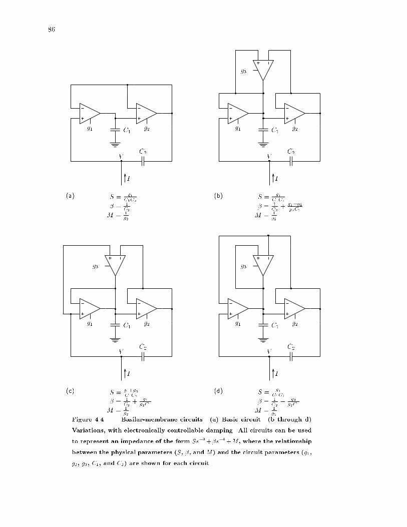
86
� = 1
C2
M = 1
g2
S = g1C1C2
S = g1C1C2
M = 1
g2
� = 1
C2+ g1�g3
g2C1
� = 1
C2+ g1
g2C1
M = 1
g2
S = g1+g3C1C2
� = 1
C2�
g3g2C1
M = 1
g2
S = g1C1C2
g1 g2C1
C2V
I
(a) (b)
I
VC2
C1g2g1
g3
g3
g1 g2C1
C2V
I
(c)
g3
g1 g2C1
C2V
I
(d)
Figure 4.4 Basilar-membrane circuits. (a) Basic circuit. (b through d)
Variations, with electronically controllable damping. All circuits can be used
to represent an impedance of the form Ss�2+�s�1+M , where the relationship
between the physical parameters (S, �, and M) and the circuit parameters (g1,
g2, g3, C1, and C2) are shown for each circuit.

87
analyzed many variations of this family of circuits [49], including nonlinear e�ects. Lyon
has found that certain undesirable nonlinear e�ects can be mitigated through the use of
third-order �lter stages [64].
The detailed transistor-level implementation of the basilar-membrane circuit is described
in Section 4.3.
4.1.3 Variation of Parameters
A resistive network and the bank of basilar-membrane circuits constitute the resistive-
network cochlear model, as shown in Figure 4.2. The membrane circuits must be tuned
in some way to simulate the decreasing sti�ness and other parameter variations of the real
basilar membrane. A simple and useful set of parameter variations, called the constant-mass
scaling con�guration, was introduced in Chapter 3, and is repeated here for convenience:
S(x) = S0 exp(�2x=d!);
�(x) = �0 exp(�x=d!);
M(x) = M0;
�(x) = �0:
An exponentially decreasing membrane parameter, such as the sti�ness, is simulated in
the electronic cochlea through the use of a tilted bias line, as shown in Figure 4.5. A long
resistive polysilicon wire runs from one end of the cochlea to the other, and the ampli�er
bias inputs are connected to it at regularly spaced intervals. When a di�erential voltage
is applied to the two ends of the wire, a linear voltage gradient appears along the wire's
length. Because of the exponential relationship between bias voltage and transconductance,
a linearly decreasing bias voltage results in an exponentially decreasing transconductance.
Finally, since the sti�ness depends linearly on the transconductance, the desired exponen-
tially decreasing sti�ness has been achieved. Constant parameters, such as the mass M in
the constant-mass scaling con�guration, are achieved easily; we simply tie both ends of the
resistive bias wire to the same voltage, or, alternatively, we bias one end and let the other
end oat. This elegant and simple method for varying circuit parameters was originally
conceived by Lyon and Mead for their unidirectional-�lter-cascade cochlear model [66]; it

88
B B B B B B
V(t)Resistive Network
V1LV2L
V1RV2R
Resistive bias wires
Figure 4.5 Tilted bias lines. An exponentially varying membrane pa-
rameter is achieved through the use of a di�erential voltage applied across a
resistive bias wire. The bias inputs to the membrane circuits are connected to
the resistive wire at regularly spaced intervals. The linear voltage drop across
the resistive wire results in an exponentially varying transconductance at each
position. We achieve constant membrane parameters by applying the same
voltage at the two ends of the bias wire.
is a prime example of how the physics of the implementation medium can be employed to
perform a useful computation.
The resistive-network cochlear model would not propagate waves using the constant-
mass scaling con�guration. The failure was due to the limited linear range of the transcon-
ductance ampli�ers in the membrane circuits. In practice, the transconductances g1 and
g2 must be approximately equal, so that the di�erential inputs to each ampli�er will be
comparable and within about a �60 mV range. This condition is in direct con ict with the
constant-mass scaling con�guration, in which g1(x) decreases exponentially with position,
and g2(x) remains constant.
As described in the Chapter 3, we may also use the increasing-mass scaling con�guration,
repeated below for convenience:
S(x) = S0 exp(�x=d!);
�(x) = �0;
M(x) = M0 exp(+x=d!);

89
�(x) = �0 exp(+x=d!): (4.5)
Although this scaling con�guration is equivalent to the constant-mass scaling con�guration
(in the sense that the corresponding solutions are identical modulo a scaling factor), it
is vastly superior for implementing the cochlear model in analog VLSI. The increasing-
mass scaling con�guration calls for both transconductances g1(x) and g2(x) to decrease
exponentially, so both ampli�ers in a given stage can be kept in their linear ranges for
small signals. Since both transconductances decrease with the same space constant d!, a
single tilted bias wire can be shared. Sharing a single bias wire between the two parameters
economizes on physical resources, improves matching of the devices, and simpli�es testing
through the elimination of redundant degrees of freedom.
In the basic membrane circuit of Figure 4.4(a), the damping term � is the one parameter
that cannot be adjusted by a transconductance. Fortunately, the increasing-mass scaling
con�guration calls for the damping to be constant. The uid mass �(x) corresponds to the
resistance of the resistive network, which can be controlled, in principle, by the same tilted
bias line that was used to control the sti�ness and mass. (For practical reasons outlined in
Section 4.3, a separate tilted bias line is used to control the resistive network.)
An important analogy between the three-dimensional biological cochlea and the resistive-
network cochlear model can now be appreciated. The decreasing membrane sti�ness, in-
creasing membrane mass, and increasing participatory uid mass of the real cochlea all
are essentially controlled by a single physical parameter: the widening basilar membrane.
Similarly, in the resistive-network model, the exponentially varying membrane sti�ness,
membrane mass, and participatory uid mass all are controlled by a single tilted bias wire.
By attempting to build a working physical model, we have discovered an important de-
sign principle: For economy, for improved matching, and for simpler testing, use a single
independently varying parameter to control all other dependently varying parameters.
4.2 Characterization of the Cochlear Model
In Section 4.1, the uid and membrane subcircuits were developed. In this section, those
subcircuits are combined, ultimately to create a full two-dimensional silicon cochlea. Since
there are nonidealities in the silicon implementation, it is important to build gradually

90
g1 g2C1
C2
I
RVin Vout
(a) (b)
R
I Zm
Vin Vout
Figure 4.6 A single cochlea stage, showing the basilar-membrane circuit
and a single resistor R from the resistive network. (a) The details of the
basilar-membrane circuit are shown fully. (b) The basilar-membrane circuit is
represented by an equivalent impedance Zm to ground.
toward the full two-dimensional model. We begin by characterizing a single stage of the
resistive-network cochlear model, containing a single basilar-membrane circuit and a single
resistor. The single stage is the smallest circuit that allows us to characterize the inter-
action between the uid and membrane circuits. Important nonideal e�ects, such as stray
capacitances and nonlinearities, appear at this level of integration.
At the next level of integration, many single stages are connected in a chain to form the
one-dimensional resistive-network cochlea. Test results from working chips are compared to
simulations to con�rm their correct operation. At the highest level of integration, the full
two-dimensional resistive-network is used to represent the cochlear uid. At this level, the
chips exhibit the short-wave and cut-o� wave propagation e�ects characteristic of cochlear
models that include the depth dimension.
Finally, the resistive-network cochlear model is compared brie y to the unidirectional-
�lter-cascade model of Lyon and Mead [66], and to the classic transmission-line circuit
model.

91
4.2.1 A Single Stage
A single stage of the one-dimensional resistive-network cochlear model is shown in Fig-
ure 4.6. The single stage contains a basilar-membrane circuit and a resistor, corresponding
to a small piece of basilar membrane and a small amount of uid. The minimal basilar-
membrane circuit of Figure 4.4(a) is emphasized from here on, but other variations also
may be used.
Note that the response of an isolated stage is di�erent from the response of a single
stage in a cascade, because of the loading of the other stages. In this section, we shall
be measuring the response of a single stage in isolation. The results will help us to build
intuition about how the uid and membrane circuits interact, and to determine the e�ects
of nonidealities within a stage; no conclusions can be drawn from the isolated single-stage
measurements about the behavior of a cascade of stages. In particular, transfer functions
cannot be multiplied to obtain the response of a one-dimensional cascade. Slaney discusses
the e�ects of multiplying transfer functions in a cascade [105].
For the isolated stage of Figure 4.6, the input is the voltage Vin applied to the left end
of the resistor, and the output is the voltage Vout measured at the right end of the resistor,
as shown in Figure 4.6. The basilar-membrane circuit was designed to simulate a particular
form of impedance to ground, as shown in Figure 4.6(b), where that impedance is
Zm =V
I=
g1
C1C2s2+
1
C2s+
1
g2:
The isolated stage is a simple voltage divider, so its transfer function can be computed
easily:
H(s) =Vout
Vin
=Zm
R+ Zm
=1 + �s=Q+ �
2s2
1 + �s=Q+ �2s2(1 + �); (4.6)
where � =p�1�2, Q =
p�2=�1, �1 = C1=g1, �2 = C2=g2, and � = Rg2. We are now empha-
sizing the functional parameters � , Q, and �, over the physical parameters C1, C2, g1, g2,
and R, since the functional parameters can be inferred more easily from chip measurements.

92
H(s) has a complex-pole pair, sp+ and sp�, located at the roots of the denominator:
sp� =1
2�Q(1 + �)
��1�
q1� 4Q2(1 + �)
�:
H(s) has a complex-zero pair, sz+ and sz�, located at the roots of the numerator:
sz� =1
2�Q
��1�
q1� 4Q2
�:
Equally important is the transfer function G(s) between the current signal I and the
input voltage Vin:
G(s) =I
Vin=
H(s)
Zm(4.7)
=1
R+ Zm(4.8)
=��
2s2
R[1 + �s=Q+ �2s2(1 + �)](4.9)
G(s) has the same complex-pole-pair as H(s), and a complex-zero-pair at the origin, as
expected, since I is the current through a capacitor.
The poles and zeros for the voltage response H(s) in the complex s-plane are shown
in Figure 4.7. The poles and zeros are close to the imaginary axis, so we should expect a
pronounced peak and a pronounced valley in the magnitude of the ideal transfer function
H.
Stray capacitances on either terminal of C2, as shown in Figure 4.8, can impair the
operation of the single stage to the point of dysfunction. For correct operation, we require
that the stray capacitances on either terminal of C2 are small compared to C2. The main
weapon in the battle against stray capacitances is the driven shield, as shown in Figure 4.8,
and described in detail in Section 4.3.
The measured voltage response H(f) is compared to the ideal response in Figure 4.9,
with and without the driven shield. The driven shield is necessary to achieve nearly ideal
responses from a single stage. We shall see in the next section that the driven shield is
indispensible in a long cascade of stages.
Features of the data correspond directly to the functional parameters � , Q, and �.
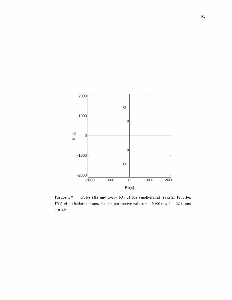
93
-2000 -1000 0 1000 2000
Re[s]
-2000
-1000
0
1000
2000
Im[s
]
X
X
O
O
Figure 4.7 Poles (X) and zeros (O) of the small-signal transfer function
H(s) of an isolated stage, for the parameter values � = 0:106 ms, Q = 3:04, and
� = 2:9.

94
g1 g2C1
C2
R Vout
(a) (b)
Vin Vin VoutR
C2
C1g2g1
Figure 4.8 Reduction of parasitic capacitances with a driven shield.
(a) The terminals of the oating capacitor C2 have parasitic capacitances to
ground, which can prevent the circuit from operating correctly. (b) The para-
sitic capacitances can be reduced signi�cantly through the use of careful layout
and of a shield that is actively driven by a fast follower. Further details are
given in Section 4.3.

95
100
1000
10000
Frequency (Hz)
-20
-10
0
10
Mag
nitu
de o
f H(f
) (d
B)
IdealWith ShieldWithout Shield
100
1000
10000
Frequency (Hz)
-0.4
-0.3
-0.2
-0.1
0
Pha
se o
f H(f
) (c
ycle
s)
Ideal
With Shield
Without Shield
(a)
(b)
Figure 4.9 Theoretical and measured small-signal voltage responses H(f)
of an isolated one-dimensional cochlea stage. (a) Magnitude. (b) Phase. The
ideal theoretical response is shown for the parameter values � = 0:106 ms,
Q = 3:04, and � = 2:9. Without the driven shield, the measured chip response
does not agree well with theory: The peak is strongly attenuated, and there
is a large droop in both the magnitude and phase responses. With the driven
shield, the measured chip response is nearly ideal; small remaining parasitic
capacitances cause the slight discrepancies from the ideal theoretical response.

96
Loosely speaking, � controls the frequency at which the valley in the magnitude response
occurs. Q controls the sharpness of both the peak and the valley. � controls the separation
between the peak and the valley. If � is too small, the peak and the valley are too close
together, and tend to cancel each other. This cancellation is evident from inspection of
Equation 4.6: for � � 1, H(s) � 1. In practice, we require � > 1 to get a reasonable
separation between the peak and valley of the transfer function. In physical terms, the
resistance R must be large, so that the small currents injected by g2 through C2 will cause
a signi�cant voltage drop across R. So we need large resistances in the resistive network
so that the basilar-membrane circuits can be e�ective. This conclusion remains true at the
system level, at which many stages are connected together.
Since � is always positive, the poles are always closer to the real axis than are the zeros,
so the peak in the magnitude of the transfer function always occurs at a lower frequency
than does the valley. For the ideal case, with no parasitic capacitances or nonlinearities,
the poles and zeros always have a negative real part (they appear in the left half-plane in
Figure 4.7), so the circuit is unconditionally stable.
The measured current response G(f) is compared to the ideal response in Figure 4.10,
with and without the driven shield. The driven shield is necessary to achieve nearly ideal
responses from a single stage.
The nonlinear behavior of the transconductance ampli�ers in the basilar-membrane cir-
cuit has an e�ect on the measured chip responses. For large signals, the e�ective transcon-
ductance of an ampli�er decreases with increasing signal amplitude, causing the peak fre-
quency to decrease, as shown in Figure 4.11. At very high amplitudes, the response becomes
multi-valued, so the measured response depends on which direction the frequency is being
swept. This frequency-domain hysteresis was �rst analyzed in the context of nonlinear
driven mechanical systems by Du�ng [25, 116, 1], and has been analyzed in the context of
analog VLSI circuits by Kerns [49].
In the real cochlea also, the peak frequency at a given place decreases with increasing
signal amplitude, but the e�ect is attributed to the nonlinear e�ects of the active outer
hair cells. The nonlinearity in the silicon implementation is more analogous to some kind
of nonlinearity in the passive basilar membrane, which is not biologically realistic. Loosely
speaking, the circuit does the right thing, but for the wrong reason. In keeping with the

97
100
1000
10000
Frequency (Hz)
-30
-20
-10
0
10
Mag
nitu
de o
f G(f
) (d
B)
IdealWith ShieldWithout Shield
100
1000
10000
Frequency (Hz)
-0.2
0
0.2
0.4
Pha
se o
f G(f
) (c
ycle
s)
Ideal
With Shield
Without Shield
(a)
(b)
Figure 4.10 Theoretical and measured small-signal current responses G(f)
of an isolated one-dimensional cochlea stage. (a) Magnitude. (b) Phase. The
ideal theoretical response is shown for the parameter values � = 0:106 ms,
Q = 3:04, and � = 2:9. The attenuation at low frequencies is caused by the zeros
at the origin, and the peak is caused by the poles. With the driven shield, the
measured chip response is nearly ideal.

98
100
1000
10000
Frequency (Hz)
-10
0
10
20
30
40
50
Mag
nitu
de o
f Vou
t (dB
re
2 m
V p
-p)
Increasing Frequency
Decreasing Frequency
5
10
15
20
25
30
35
40
45
50
Figure 4.11 The saturating nonlinearity in a single stage of the one-
dimensional resistive-network cochlear model. The input amplitude in dB
relative to 2 mV p-p is marked on each curve. At each amplitude, the fre-
quency response was measured for an increasing frequency sweep and a de-
creasing frequency sweep. The nonlinearity causes the peak to bend toward
lower frequencies when the output amplitude exceeds about 150 mV p-p. At
very high amplitudes, the frequency response becomes multivalued, resulting
in a frequency-domain{hysteresis e�ect: The response near the peak depends
on the direction of the frequency sweep.

99
R R RRRR
B B B B B B
Vin
V(n)
I(n)
Figure 4.12 One-dimensional cochlear circuit model. The two-dimensional
resistive network of Figure 4.2 has been collapsed into a single chain of resis-
tors. The input signal Vin is applied to the left end of the cochlea. The outputs
are the voltage V (n) and the current I(n) owing into the membrane circuit at
each stage n.
philosophy of modeling the biology faithfully, the cochlea circuit should be operated with
small signals, so that the behavior of the electronic basilar membrane remains linear; the
nonlinearity due to the outer hair cells should be modeled by a separate circuit, as described
in Chapter 5.
4.2.2 The One-Dimensional Cochlear Model
The one-dimensional cochlear model consists of a chain of cochlear stages, as shown in
Figure 4.12. The results presented here are for a cochlea chip with 64 stages. The input
signal Vin is applied to the left end of the cochlea. The outputs of the cochlea are the
voltage at each stage, corresponding to the velocity potential of the uid, and the current
owing into the membrane circuit at each stage, corresponding to the basilar-membrane
velocity. The output voltages and currents were observed via an analog-signal multiplexer,
or scanner [72].
The measured and simulated frequency responses for every �fth voltage tap of a 64-
stage cochlea are shown in Figure 4.13. The voltage responses show a at behavior for
low frequencies, followed by a sharp cut-o� at high frequencies, with slopes up to 400
dB/decade. Both the simulated response and the measured responses show large ripples
at very low frequencies, as a result of re ections from the helicotrema end. The measured
response shows small ripples at all frequencies. Simulations indicated that these ripples
were related to parasitic capacitances in the chip.

100
100
1000
Frequency (Hz)
-50
-40
-30
-20
-10
0
Gai
n (d
B)
100
1000
Frequency (Hz)
-50
-40
-30
-20
-10
0
Gai
n (d
B)
(a)
(b)
Figure 4.13 Magnitude of frequency response of every �fth voltage tap,
from tap 10 to tap 60, in a 64-stage cochlea. Tap 10 occupies the upper-right
part of each graph. (a) Chip response. Parameters: TAUL = 4.25 V, TAUR =
4.42 V, RL = 1.08 V, RR = 0.629 V, IOL = 0.143 V, IOR = 0.268 V, QCONT
= 5.08 V. (b) Simulated response. Parameters: FOL = 4680 Hz, FOR = 162
Hz, Q = 2.54, ETAL = 1.07, ETAR = 0.19 V.

101
100
1000
Frequency (Hz)
0.0
-0.5
-1.0
-1.5
-2.0
-2.5
-3.0
Pha
se (
cycl
es)
100
1000
Frequency (Hz)
0.0
-0.5
-1.0
-1.5
-2.0
-2.5
-3.0
Pha
se (
cycl
es)
(a)
(b)
Figure 4.14 Phase of frequency response of every �fth voltage tap, from
tap 10 to tap 60, in a 64-stage cochlea. Tap 10 occupies the upper-right part
of each graph. (a) Chip response, for the same parameters as in Figure 4.13.
(b) Simulated response, for the same parameters as in Figure 4.13.

102
The phase response for the voltage signals at every �fth tap are shown in Figure 4.14. It
was possible to achieve about 2 or 2.5 cycles of phase accumulation, so a genuine traveling
wave is observed.
The current responses at every �fth tap are shown in Figure 4.15. They show a gentle
rise for low frequencies, with a sharp cut-o� at high frequencies. The uneven appearance
of the peaks in the current response is due to random multiplicative factors in the current
mirrors used to copy out the current.
In Figure 4.16, the current-tap peak frequency is shown as a function of tap number.
There is clearly a downward trend, although the response is not monotonic.
The current response of tap 36 is shown in Figure 4.17. The response is approximately
linear over a large range. Finally, the e�ect of the driven shield is shown in Figure 4.18.
Without the driven shield, the response is strongly attenuated.
The power consumption of the chip is 8 mW with the scanner running at 1 MHz.
These experimental results con�rm the correct operation of the individual subcircuits
and of the system as a whole, in the one-dimensional special case. We now turn to the
two-dimensional case.
4.2.3 The Two-Dimensional Cochlear Model
The two-dimensional cochlea circuit model is shown conceptually in Figure 4.2. The fab-
ricated circuit consists of a 61 � 5 resistor array, with 61 basilar-membrane circuits. The
output signals are the voltages at each node of the resistive network, and the current owing
into each basilar-membrane circuit. The output voltages and currents were observed via an
analog-signal multiplexer, or scanner [72].
Since the correct operation of the membrane and resistor circuits was veri�ed in the
one-dimensional model, the primary purpose of testing the two-dimensional model is to
investigate the wave propagation behavior that is speci�c to the depth dimension|that is,
to con�rm that short-wave and cut-o� behavior can be produced by the analog VLSI model.
Figure 4.19 shows the voltage response in decibels as a function of position in the grid,
for a �xed frequency. The voltage at each point is analogous to the velocity potential, which
is proportional to uid pressure at a given frequency. At the basal end (taps 1 through 30),
the wave is long, and the amplitude of voltage does not depend on the height. On taps 30

103
100
1000
Frequency (Hz)
-40
-30
-20
-10
0
Gai
n (d
B)
100
1000
Frequency (Hz)
-40
-30
-20
-10
0
Gai
n (d
B)
(a)
(b)
Figure 4.15 Magnitude of frequency response of every �fth current tap,
from tap 10 to tap 60, in a 64-stage cochlea. Tap 10 occupies the upper-
right part of each graph. (a) Chip response, for the same parameters as in
Figure 4.13. Each tap is multiplied by a random gain factor, due to mismatch
in the current mirrors used to make the current signal observable. The mirrors
have been tilted; that is, greater gain is applied to the later taps, to keep the
peak response at each tap approximately constant. The current response is
inferred from the voltage across a linear resistor in a current-sense ampli�er,
so all curves are also scaled by a constant factor. (b) Simulated response, for
the same parameters as in Figure 4.13. Low-frequency taps have been scaled
to keep the peak response approximately constant.

104
10 20 30 40 50 60
Tap Number
100
1000
Bes
t Fre
quen
cy (
Hz)
Figure 4.16 The variation of best frequency with tap number, for taps 10
to 60 of a 64-stage cochlea, using the same parameters as in Figure 4.13. The
best frequency decreases approximately exponentially with distance. For refer-
ence, a best-�t straight line is superimposed, corresponding to an exponential
decrease. Note that the decrease is not monotonic.

105
100
1000
Frequency (Hz)
-10
0
10
20
30
40
50
Res
pons
e (d
B)
Figure 4.17 Frequency response of tap 36 at di�erent amplitudes, using the
same parameters as Figure 4.13. The input amplitudes range from 5 dB to 45
dB, with respect to 2 mV p-p. The response shows linear behavior over a wide
range of input amplitudes, and then begins to show a slight downward-shifting
peak frequency for higher amplitudes.
100
1000
Frequency (Hz)
-50
-40
-30
-20
-10
0
Res
pons
e (d
B)
With ShieldWithout Shield
Figure 4.18 The e�ect of the driven shield on tap 36 of the one-dimensional
cochlea. The parameters are the same as in Figure 4.13. Without the driven
shield, the signal is highly attenuated.

106
0 10 20 30 40 50 60
Tap Number
-60
-50
-40
-30
-20
-10
0
Gai
n (d
B)
Row 5 (y=h)Row 4 Row 3 Row 2Row 1 (y=0)
0 10 20 30 40 50 60
Tap Number
-2.5
-2
-1.5
-1
-0.5
0
Pha
se (
cycl
es)
Row 5 (y=h)Row 4 Row 3 Row 2Row 1 (y=0)
(a)
(b)
Figure 4.19 Voltage measurements along the �ve rows of the resistive net-
work, for a 230 Hz input. (a) Gain (dB). (b) Phase (cycles). Long-wave
behavior is evident from taps 1 through 30, where all �ve rows have equal re-
sponses (response does not depend on depth dimension). Short-wave behavior
is evident from taps 30 through 50, where the �ve rows diverge (response does
depend on depth dimension). Chip parameters: TAUL = 4.10 V, TAUR =
4.15 V, RL = 0.911 V, RR = 0.606 V, QCONT = 4.92 V.

107
through 50, the wave begins to become short, so that the wave amplitude does depend on
the height; the amplitude at the bottom of the uid begins to fall o� more rapidly than at
the top. A notch is evident in the response near the bottom of the uid, corresponding to
the cut-o� conditions where the lowest wavenumber mode begins to dominate.
In Figure 4.19(b), the phase curves split into three groups, separated by about one cycle.
This behavior is the result of the gradual dominance of the cut-o� mode and the periodicity
of the phase function. Di�erent rows accumulate more phase in the traveling-wave mode
before the cut-o� mode becomes dominant; at the crossover point, the phase curves are
pulled to the phase of the cut-o� mode, modulo the nearest integer-cycle o�set.
To allow visualization of the complex two-dimensional behavior of the uid pressure, the
data of Figure 4.19 are plotted as an intensity grid in Figure 4.20. Finally, the magnitude
data are shown as a surface plot in Figure 4.21, to illustrate the notch associated with
destructive interference of the traveling-wave and cut-o� modes.
4.2.4 Comparison to Other Circuit Models
The resistive-network cochlear model has many important similarities to the unidirectional-
�lter-cascade model of Lyon and Mead [66, 125], and to the classic transmission-line model
[85]. In this section, the models are compared.
Comparison to the Unidirectional-Filter-Cascade Model
The resistive-network cochlear model and the unidirectional-�lter-cascade model are shown
in Figure 4.22. For brevity, in this section, the names of the two models will be abbreviated
to RNC (resistive-network cochlea) and UFC (unidirectional �lter cascade).1
Like the RNC model, Lyon and Mead's UFC model was designed for implementation in
analog VLSI technology. Tilted bias lines are used to control the speed and wavelength of
propagating waves in the UFC model, as in the RNC model. The high-impedance input of
each UFC stage permits waves to propagate in the forward direction only, whereas waves
can propagate in both directions in the RNC model. In a cascade of UFC sections, later
stages do not load earlier stages; hence, the transfer function of a cascade is simply the
1The two cochlear models are sometimes called New Cochlea and Cochlea Classic, respectively. So far,
we have not found a design compact enough to be worthy of the name Diet Cochlea.

108
0
5
0
5
0
5
0
5
0
5
0
5
0
5
0 10 20 30 40 50 600
5
Tap Number
Row Number Phase(cycles)
0
1/8
1/4
3/8
1/2
5/8
3/4
7/8
Figure 4.20 Chip data, showing the real part of uid pressure at a �xed
frequency, at eight phases to allow visualization of the traveling wave. Positive
uid pressure is indicated by light values; negative uid pressure is indicated
by dark values. Resting pressure is indicated by medium gray. Long-wave
behavior is evident for taps 1 through 30. Short-wave behavior is especially
visible around taps 45 through 50. Beyond tap 50, the wave amplitudes are
too small to be seen in this representation. The chip parameters are the same
as in Figure 4.19.

109
20
40
60
Tap
12345
Row
-40-200
|Gain| (dB)
20
40
60
Tap
12345
R
-4-20
Figure 4.21 Magnitude of the voltage signal at all positions in the resistive
network. The data are plotted as a surface to illustrate the notch associated
with destructive interference of the traveling-wave and cut-o� modes. This
�gure may be compared to Figure 3.15.
C g�g�
gQg1 g2C1
C2
I
RVin Vout
(a) (b)
C
Vin Vout
Figure 4.22 Comparison of the resistive-network cochlear model and Lyon
and Mead's unidirectional-�lter-cascade model. (a) A single stage of the one-
dimensional resistive-network model. (b) A single stage of the unidirectional-
�lter-cascade model.

110
product of the transfer functions of the constituent stages. This simple analysis technique
does not apply to the RNC model, which requires the LG technique or numerical solutions
to account for the interactions between stages. The transfer function of an individual UFC
stage contains a conjugate-pole pair only, whereas an isolated RNC stage contains both
poles and zeros. Since there are no oating capacitors in the UFC model, there are no
signi�cant problems with parasitic capacitances, as there are in the RNC model. Nonlinear
e�ects in the UFC model have been analyzed extensively [71, 125, 64, 49].
A typical UFC stage occupies an area of 100�m � 100�m, whereas a typical RNC
membrane circuit occupies about 10 times as much area. The greater area is primarily due
to the stray-capacitance-reduction techniques outlined in Section 4.3. In a two-dimensional
RNC model, the resistive network increases the total chip area further still.
Since the UFC stages can be tuned to achieve greater-than-unity gain over some fre-
quency range, the UFC model can be used to model ampli�cation of waves in the cochlea,
corresponding roughly to the ampli�cation due to the outer hair cells. The Q, or degree
of resonance, of each UFC stage is a very sensitive function of the transconductance gQ.
Mismatch between ampli�ers causes some stages to be inherently more lightly damped than
others; to keep these worst-case sections stable, we must damp the entire line heavily. Pro-
posed solutions to this problem include alternate feedback con�gurations that are more
robust in the presence of device mismatch, and adaptive control of the existing feedback, to
allow lightly damped stages to increase their own damping. The RNC model, as described
so far, does not contain any elements to model active e�ects.
Device mismatch can cause a random constant voltage o�set to appear at the output
of each UFC stage. Systematic o�sets due to nonideal current mirrors can cause the DC
operating point of the cascade to drift toward one of the power supply rails. The systematic
o�sets in the UFC model can be reduced by careful design, but they cannot be eliminated
entirely. By comparison, the RNC model performs an o�set-free computation; the resistor
elements have no DC o�sets, and the DC o�sets in the membrane-circuit ampli�ers are
isolated from the resistive network by the capacitor C2.
The serial UFC cascade has a very low tolerance for component failure, since one dead
section will block signal transmission to the following stages. The two-dimensional RNC
model presented in this dissertation degrades more gracefully with component failure, at

111
the expense of considerably greater layout area.
A �nal interesting comment on the UFC model relates to spatial resolution: how many
stages should be used to build a cochlea? It is tempting to guess that \more is better," but
Feinstein has pointed out that there is no continuum limit for the UFC model [30]; in the
limit of an in�nite number of stages, there will be an in�nite delay from the input to any
particular place in the UFC cascade. Since the RNC model is a discrete approximation of
a continuous physical model, adding stages to it simply improves the approximation, so a
continuum limit does exist for the RNC model.
In the present VLSI fabrication environment, in which chips are limited to a size of
about 1 cm � 1 cm, the compactness issue is a strong feature in favor of the UFC model. If
we want to have any room to build any higher-level neural processing circuitry on the chip,
we had better make the cochlea itself as small as possible. However, with the development
of improved chip-to-chip communication protocols, pioneered by Mahowald [68], it is likely
that, in the next few years, cochlea chips will be designed with a standard interface, and
neural processing will be implemented on some other chip. When an entire chip can be
devoted to the cochlea, the compactness issue will become less important, and the continuum
limit issue will become more important, so the balance will swing more evenly to the RNC
model. As wafer-scale integration becomes a possibility in the next 5 to 10 years [29], the
compactness issue will recede and the fault-tolerance and continuum-limit issues will become
paramount, so the RNC model may be preferable to the UFC model for some applications.
Comparison to the Transmission-Line Model
The one-dimensional resistive-network cochlear model is related in an interesting way to
the transmission-line model [85]. For ease of comparison, the two models are shown in
Figure 4.23, where the resistive-network model has been drawn to emphasize the series
resistance R and the equivalent impedance Zm of the basilar membrane circuit.
The transfer function of an isolated stage of the transmission-line model is
H(s) =Vout
Vin=
1 + �s=Q+ �2s2
1 + �s=Q+ �2s2(1 + �); (4.10)
where � =pL=C, Q =
qRLC
, and � = L1=L. This transfer function has the same form

112
(a) (b)
L1Vin VoutVoutVin
Zm
R
L
R
C
Figure 4.23 Comparison of the resistive-network cochlear model and the
classic transmission-line model. (a) A single stage of the one-dimensional
resistive-network model. The membrane circuit is represented by its equiva-
lent impedance Zm, as in Figure 4.6. (b) A single stage of the transmission-line
model.
as Equation 4.6, and hence, the transmission-line and resistive-network models propagate
waves of the same form. However, the signal representations in the two circuits are di�erent.
In the transmission-line model, the voltage signal is analogous to uid pressure, and the
current signal owing through the series impedance to ground is analogous to membrane
velocity. In the resistive-network model, the voltage signal is analogous to velocity potential,
and the current signal is proportional to membrane velocity.
There is a deeper principle here that will allow us to build at least two other equiva-
lent circuits. Recall that the resistive network solves Laplace's equation, and thus can be
used to represent the incompressible cochlear uid. But we can show easily that an induc-
tive network also solves Laplace's equation. In fact, we can build the network out of any
impedance elements we like, and it will still solve Laplace's equation. It does not matter
what the elements are, as long as they are all the same. So we could, in principle, build a
cochlear model in which the uid was represented by a capacitive network, or by a negative-
resistance network. Although negative-resistance networks seem doomed to have stability
problems, two-dimensional capacitive networks seem to present a practical possibility. The
two immediately obvious problems with a capacitive network are the parasitic capacitances
and the di�culty in controlling the DC operating point of the membrane circuit.
Although the transmission-line model is based on the idea of representing the cochlear
uid mass by inductances, it is usually discussed in the one-dimensional case [137, 98, 134,

113
Series Transistors
Bias Circuit Bias Circuit
V2
Vb Vb
V1
Figure 4.24 Mead's resistor circuit. This circuit provides a linear resistance
between the nodes marked V1 and V2, for voltage di�erences less than about 60
mV. The resistive path is created by the pair of transistors in series. The bias
circuits allow the resistance to be relatively independent of the DC operating
point.
59]. The extension to a two- or three-dimensional inductive network is obvious, but Kolston
was the �rst worker to mention it explicitly [54, p. 72]. In analog VLSI technology, inductors
cannot be be built directly, although they can be simulated with gyrator circuits or current
conveyors [100, p. 113].
4.3 Analog VLSI Implementation
In this section, we consider the transistor-level circuits used to implement the cochlear
model in analog VLSI.
4.3.1 Resistor Circuit
Many designs were investigated for the resistors in the resistive network [124, 5]. The best
performance was found with the resistor circuit designed by Mead [71] for use in the silicon
retina of Mahowald and Mead [69]. The circuit is shown in Figure 4.24. A resistance

114
between two points is implemented by a pair of transistors in series. The innovation of
the circuit is the use of a bias circuit to keep the conductance of the series-transistor pair
approximately constant over a wide DC operating range. The circuit has been analyzed
extensively by Mead [71, pp. 116-119]. The e�ective resistance of the circuit is proportional
to exp(��Vb=UT), where Vb is the externally applied bias voltage, and the thermal voltage
UT is about 25 mV at room temperature. The parameter � relates to the e�ectiveness of
the bias voltage in controlling the current owing in the bias circuit. A typical value of �
is 0.7.
The function of the bias circuits is to compute a voltage for the gate of the series
transistors such that the conductance of the series transistor in approximately constant over
a wide range of input voltages. This remarkable invariance must be achieved in the presence
of the back-gate e�ect [71]; the net result is that the voltage computed by the bias circuit
may be considerably larger than the input voltage. In practice, for the computed voltage
to lie below the 5V power supply, we must restrict the DC operating level of the resistive
network to below about 3 V. We shall see shortly that this requirement is incompatible
with the required operating range of the membrane circuit. We can remedy this problem
by reversing the polarity of the entire resistor circuit|that is, by replacing all native-type
devices with well-type devices, and reversing power and ground. Such a well-type resistor
circuit will operate correctly as long as the input voltage is above about 2 V.
In the rectangular resistive network, there are four resistors connected to each node.
However, there is no need to build four bias circuits at each node. For e�ciency and im-
proved matching, it is preferable to share one bias circuit between the four series transistors
associated with each node. Since the resistance of the circuit varies exponentially with the
bias voltage Vb, we can use a linearly tilted bias line to achieve an exponentially increasing
resistance, to correspond roughly with increasing participatory uid mass in the modi�ed
two-dimensional cochlear model.
4.3.2 Basilar-Membrane Circuit
A detailed transistor-level schematic diagram of the basilar-membrane circuit is shown in
Figure 4.25. The basic element of the circuit is the transconductance ampli�er, described
in detail by Mead [71]. Diode-connected transistors have been included beneath the input

115
Ampli�er 1 Ampli�er 2 Copy
Fast Follower Driven Shield
TAU
QCONT
IOCONT
IOUT
FAST
VOUT
VIN
Figure 4.25 Detailed transistor-level schematic diagram of the basilar-
membrane circuit of Figure 4.4(a). The VIN node connects to the resistive
network. A common bias line TAU is used for Ampli�ers 1 and 2, so that there
will be a �xed ratio between the transconductances of the two ampli�ers, re-
gardless of the tilt on the TAU line. The QCONT input allows the ratio of the
two transconductances to be controlled globally. Both ampli�ers have source-
degeneration diodes to widen their linear range. The current owing out of
Ampli�er 2 is duplicated using the \copy" transistor. IOUT is proportional
to the bidirectional current I plus a constant current. The IOCONT input
to Ampli�er 2 allows IOUT to be scaled by a large factor, for easier o�-chip
sensing. The fast follower serves two purposes. It provides a bu�ered replica
of the VIN signal for o�-chip measurements, and drives the shield used to
reduce strays on the oating capacitor.

116
transistors of ampli�ers 1 and 2 to increase the linear operating range from about 50 mV
p-p to about 200 mV p-p [125]. This technique is called source degeneration because the
ability to control the current in an input transistor is degenerated by the placement of an
impedance in the source of that transistor.
The bias control TAU is shared between ampli�ers 1 and 2, to enforce a �xed ratio be-
tween the transconductances of the ampli�ers, regardless of the tilt on the TAU line. The
source-control knob QCONT on the �rst ampli�er allows the ratio of the two transconduc-
tances to be controlled globally.
A single transistor makes a copy IOUT of the current I owing into the circuit from
the resistive network. IOUT is equal to a scaled version of I plus a constant current. The
amount of scaling is controlled by the IOCONT input to ampli�er 2 [125].
The fast follower serves two purposes. It provides a bu�ered replica of the VIN signal
for o�-chip measurements, so that VIN can be measured without capacitively loading the
circuit. The fast follower also drives the shield used to reduce parasitic capacitances to
ground on the two terminals of the oating capacitor.
4.3.3 Reduction of Parasitic Capacitance
The highest interlayer capacitance available on the standard double-metal double-poly pro-
cesses o�ered by MOSIS is between the layers poly1 and poly2, with a value of about 0.58
fF/�m2. So the natural way to build the oating capacitor is to design two large overlapping
plates of poly1 and poly2, as shown in Figure 4.26(a). However, the parasitic capacitance
between poly1 and substrate is about 0.067 fF/�m2, about 12 percent of the desired value.
We shall call this capacitance the relative parasitic capacitance, since it increases in relation
to the size of the intended capacitance. In addition, there are �xed parasitic capacitances
associated with the gates of transistors, and with di�usion regions in the resistor circuits,
that can total as much as 0.5 pF on either terminal of the oating capacitor.
System-level simulations of the one-dimensional cochlea model indicate that, for correct
operation, the total parasitic capacitances must be less than 2 percent of the intended
oating capacitance. We can reduce the parasitic/intended capacitance ratio to this low
level by decreasing the relative parasitic capacitances were decreased through the use of
a driven shield, by minimizing the �xed parasitic capacitances by careful layout, and by

117
(a)
(b)
Substrate
Substrate
Silicon Dioxide
Silicon Dioxide
Poly1Poly2
Poly1Poly2
Metal1
Metal2
Well
Figure 4.26 Reduction of parasitic capacitances with a driven shield. (a) A
simple poly1-poly2 capacitor. There is a parasitic capacitance between poly1
and the substrate, about 12% of the value of the intended poly1-poly2 ca-
pacitance. (b) The driven shield. The poly2 plate of the capacitor is sand-
wiched between poly1 and metal1, which are tied together; thus, the intended
capacitance is increased slightly due to the poly2-metal1 interlayer capaci-
tance (about 7% of the poly1-poly2 interlayer capacitance). The poly1 plate
is bu�ered by a fast follower, which drives the metal2 and well layers com-
pletely enclosing the entire structure. The voltage on the poly1-metal1 plate
is surrounded by a copy of itself, so the e�ective parasitic capacitances are
neutralized.
118
increasing the intended capacitance. The implementation of the driven shield is shown in
Figure 4.26.
Assuming that the relative parasitic capacitances have been neutralized, the remaining
capacitances now dominate. Their value is the order of 0.5 pF; if we are to to ensure that the
intended oating capacitance exceeds that amount by a factor of 50, the oating capacitance
must be about 25 pF, corresponding to a huge layout area of 220�220�m. A typical cochlea
stage has layout dimensions 180�780�m, about 80 percent of which is devoted to the large
capacitors and driven shields. Even with such large capacitors, it is possible to obtain over
300 stages of a cochlea on a single MOSIS chip, including scanner. This approach has been
used to prove the feasibility of the concept. However, such a large area is not practical for
a commercial design. Another approach, presently under development, is to implement an
active stray-reduction circuit to cancel the stray capacitance.
4.3.4 DC Operating Point
Conventional transconductance ampli�ers have a common-mode operating range of about
1 to 4.5 V when biased below threshold with a 5 V power supply. Source degeneration, as
used in ampli�ers 1 and 2 of the basilar-membrane circuit, restricts the typical common-
mode operating range to 2.5 to 4.5 V [125]. The circuit is normally operated with an input
DC level of 3.5V.
We saw earlier that conventional native-type resistor circuits could operate only between
about 1 and 3 V. There is only a small voltage range in which the native-type resistors and
the basilar-membrane circuits will both function correctly. We can make the two circuits
compatible by using well-type resistor circuits, which are restricted to operation between
about 2 to 4 V.
The question of DC operating point relates to the helicotrema boundary condition.
Strictly speaking, the x derivative of voltage should vanish at the right end of the resistive
network, and thus the end should be left oating. However, at the very low current levels
required to model the lowest frequencies of hearing, leakage currents can lead to a slight
drift in the DC operating point of the neighborhood of the oating end. It is useful, in
practice, to apply a DC voltage to the right end. Of course, there is no e�ect for waves
that cut o� before they reach the end, but strictly speaking, the boundary condition is not
119
correct, and there are re ection e�ects for very low frequency waves, as seen in Figure 4.13.
4.3.5 Instrumentation, Fabrication, and Testing
In the two-dimensional cochlea chips, there are 305 voltage signals and 61 current signals
to observe externally, but there are only 28, 40, 65, or 84 pins on the standard packages.
In practice, the signals are observed through the use of an on-chip analog multiplexer, or
scanner [72]. Developed originally to allow generation of video signals from the silicon
retina, a scanner can be used also to create one-dimensional traveling-wave animations for
viewing on an oscilloscope. Combined with externally generated clock signals, the scanner
can be used as an automatic data-acquisition tool, to allow frequency responses at every
tap to be measured under computer control. All the data presented in Section 4.2 were
acquired automatically.
At the present time, the setting of chip parameters is done by hand. Kirk, Fleischer,
Watts and Barr have described a preliminary system for automated parameter setting [53].
In their system, the desired performance and error metric are speci�ed, along with an initial
parameter setting. Improved parameters are determined iteratively by gradient descent, or
through the use of special knowledge of the problem.
All data in this dissertation were taken from chips fabricated on the Orbit 2-�m double-
poly double-metal p-well process, via the MOSIS service. Single-section data are from
circuits laid out on the TinyChip frame (2.22 mm � 2.25 mm die). Multisection data are
from circuits laid out on the 4.6 mm � 6.8 mm die.
4.4 Summary
In this chapter, an electrical circuit has been presented that is an exact analog of the of the
passive two-dimensional cochlear model described in Chapter 3. The circuit uses a resistive
network to model the incompressible cochlear uid, and uses a special-purpose circuit to
model the basilar membrane. The circuit exhibits the wave propagation characteristics
predicted by numerical and analytical methods. The silicon cochlea has been fabricated in
analog VLSI CMOS technology and has been tested successfully.

120
Chapter 5
Toward an Analog VLSI Model
of Active Cochlear Mechanics
Although the majority of hearing researchers believe that the outer hair cells are responsible
for the active and nonlinear behavior of the cochlea, there is no consensus on the detailed
mechanism by which the outer hair cells in uence the propagation of cochlear waves. How-
ever, a number of plausible proposals have been made in the literature. The key ideas in
the development of modern understanding of the active processes in cochlear mechanics are
summarized below.
5.1 Review of Previous Active Models
The �rst suggestion of active processes in the cochlea was made in a visionary paper by
Gold in 1948 [38, 39]. Although Gold relied heavily on the (incorrect) \resonance" model
[37], he reasoned (correctly) that the frequency selectivity of the cochlea could not be
achieved by a purely passive system, and thus, some positive mechanical feedback must
be present to counteract the inherently high damping of the passive system. He predicted
that the cochlear microphonic was the result of a uctuating load on an electrochemical
power source [38, p. 495]. He predicted that oscillations could occur in the active mechanical
system, but was unable to measure those oscillations (Kemp was the �rst worker to measure

121
otoacoustic emissions in 1978 [48]). Gold predicted an amplitude-dependent shift in best
frequency at a given place [38, p. 497]. Finally, he observed cautiously that the hair cells
were suitably positioned to act as mechanical e�ectors [38, p. 496]. This truly visionary
work went unrecognized for three decades!
Many models have contributed to the modern understanding of nonlinear and active
cochlear mechanics [52, 80, 77, 16, 81, 75, 34, 76, 35, 55, 130, 133]. The essential ideas in
most modern models are listed below.
1. The outer hair cells are responsible for the observed nonlinearity. The basilar mem-
brane and remaining cells in the organ of Corti are linear.
2. The outer hair cells are the active (energy-producing) elements in the organ of Corti.
The basilar membrane and remaining cells in the organ of Corti are mechanically
passive.
3. Because the tips of the tallest stereocilia of the outer hair cells are attached to the
tectorial membrane, the outer hair cells are stimulated in proportion to their stereocilia
displacement, which is proportional to the displacement of the basilar membrane.
4. The outer hair cells respond to displacement of their stereocilia by exerting a force on
the basilar membrane.
5. The outer hair cells are limited in how much force they can exert on the basilar
membrane. For quiet sounds, the outer hair cells can amplify the wave signi�cantly,
whereas for louder sounds, the outer hair cells are too weak to have much e�ect. The
net result is that the forces exerted by the outer hair cells saturate at high ampli-
tudes; this component-level saturation leads to the system-level saturation observed
by Rhode [91].
6. The outer hair cells are assumed to be capable of providing forces on a cycle-by-cycle
basis at audio frequencies. Evidence for this assumption is accumulating [97]. If this
statement is true, the outer hair cells would be among the fastest-moving biological
mechanical e�ectors in existence.
The above general ideas are very plausible and are not controversial. However, it is not
clear exactly what type of force the outer hair cells are exerting on the basilar membrane.

122
Most modelers assume that the outer hair cells exert a force in phase with the velocity of
the basilar membrane in a critical region just before the best place|that is, they act like a
negative damping [16, 81, 77].
How might this negative damping be achieved? The most commonly held view is that
upward de ection of the basilar membrane causes a shearing motion of the reticular lamina
and the tectorial membrane, causing the stereocilia of the outer hair cells to be bent away
from the spiral sulcus, as shown in Figure 2.11. Ashmore has shown, in vitro, that bending
the outer-hair-cell stereocilia in that direction leads to depolarization of the cell membrane,
and that depolarization of the cell leads to a decrease in the length of the cell, which
would presumably lead to an upward force on the basilar membrane relative to the tectorial
membrane [4].
This complicated chain of events results in an upward force in response to an upward
displacement of the basilar membrane, which acts to reduce the inherent restoring force of
the basilar-membrane sti�ness. Since the force and the stimulus have the same direction,
this model is called a positive-feedback model [76]. However, Ashmore has also shown that
there is a time delay frommembrane de ection to applied force. For very low frequencies, the
time delay is negligible, and the exerted force looks like a negative sti�ness. At a particular
higher frequency, however, the time delay will correspond to a quarter-cycle phase shift,
and the force will be acting in anti-phase with the membrane velocity|the force acts like a
positive damping. At a higher frequency still, the phase shift will increase to a half-cycle,
and the force will appear as a positive sti�ness. At a three-quarter cycle phase shift, the
applied force will be in phase with the membrane velocity, and the negative damping is
achieved.
The requirement of a three-quarter cycle phase shift is quite severe; it would be simpler
if only a one-quarter cycle were required to achieve negative damping. The active-sti�ness
model of Mountain, Hubbard, and McMullen [77] assumes a negative feedback of forces to
the basilar membrane|that is, at very low frequencies, upward displacement of the basilar
membrane leads to a downward force on the basilar membrane by the outer hair cells, thus
increasing the e�ective sti�ness. At higher frequencies, a phase shift of a quarter-cycle
leads to a force that is in phase with the membrane velocity, thus decreasing the e�ective
damping.

123
At this time, it is not clear exactly how the issue will be resolved. There are several
possibilities.
1. If the upward de ection of the basilar membrane does lead, in fact, to a downward
force, the negative-feedback model of Mountain, Hubbard, and McMullen would be
vindicated, and Ashmore's micromechanical argument would have to be revised.
2. If Ashmore's positive-feedback description is correct, the negative damping still may
be achieved through the application of a three-quarter-cycle phase shift. In this case,
the negative-feedback model would have to be rejected.
3. It is possible that a completely di�erent mechanism is dominant. Kolston, for example,
has argued on the basis of energy e�ciency that the outer hair cells should act so as
to a�ect only the sti�ness or mass components of the basilar-membrane impedance
[55]. Zweig has suggested that an outer-hair-cell force with a slow-acting and a fast-
acting component may be more appropriate [133]; this suggestion �nds support in the
measurements of Ashmore [4].
Still other ingenious arguments may surface before the issue is resolved.
Nearly all of the models use pure delays in the implementation of the outer-hair-cell
mechanical input-output relationships. While pure delays are very easy to implement in
a computer simulation, they are very di�cult to implement in a physical medium, and
it is most unlikely that the outer hair cells can be modeled accurately in such a way. A
more reasonable assumption would be that the outer hair cells respond with a �rst- or
second-order �ltered version of their input stimulus.
5.2 The Outer Hair Cell Model
At this point, the most reasonable course of action is to build a exible model that will
allow investigation of all the proposed ideas. The outer hair cell model should take as its
input a signal proportional to membrane displacement. It should provide a �ltered version
of that signal, thus introducing a frequency- and place-speci�c delay. The �ltered version
should saturate at high displacement levels. Ultimately, there should be a mechanism for

124
feeding back the �ltered and saturated signal as a force acting on the basilar membrane. A
exible model would allow for both positive and negative feedback.
5.2.1 Mathematical Description
Recall that the basilar membrane boundary condition for the passive cochlear model was
given in Equation 3.8:
M(x)@2�
@t2= 2�
@�
@t� S(x)� � �(x)
@�
@tat y = h: (5:1)
In the active case, we require an additional term FH to represent the force generated by
the outer hair cells:
M(x)@2�
@t2= 2�
@�
@t� S(x)� � �(x)
@�
@t+ FH(�; !; �H(x); QH; �s; G(x)) at y = h: (5:2)
The force FH should be proportional to a delayed and saturated version of the displacement
signal �. We now consider each of these features in turn.
The conceptual model calls for a frequency- and place-speci�c delay, which can be mod-
eled most reasonably by a low-pass or band-pass �lter. The parameters of the low-pass or
band-pass �lter are �H(x) and QH , where we have implicitly assumed a second-order �lter.
Since the outer hair cells and their stereocilia increase in length from base to apex, it is
reasonable to assume that the time-constant �H increases with position x. For simplicity,
we will assume that QH is constant everywhere.
The conceptual model calls for a saturating nonlinearity, since there must be an upper
limit on the magnitude of the force that can be produced by an outer hair cell. A simple
saturating nonlinearity is the hyperbolic tangent function (also called a Boltzmann function
[130], and closely related to the Fermi-Dirac distribution function [117, p. 71]), which will
require a parameter �s to control the magnitude of displacements at which the saturating
e�ect becomes noticeable|that is, the \width of the tanh." Finally, the scaling factor G(x)
controls the magnitude of the delayed and saturated force.
Combining these terms leads to the following form of the outer hair cell force:
FH = �G tanh
�F (�; !; �H; QH)
�s
�; (5:3)

125
where the � sign allows the exibility for either positive or negative feedback, and the
function F represents the �ltering operation.
It is tempting to assume a harmonic time dependence with frequency !, and to write
the �lter operator explicitly:
FH = �G tanh
"�
�s
1
1 + i!�H=QH � !2�2H
!#: (5:4)
However, this step is not justi�ed because of the nonlinearity. For this reason, we cannot
speak of the \impedance of the organ of Corti," since the notion of an impedance is a
linear-systems concept.
Diependaal and Viergever point out that the driving function at the stapes must be
handled with considerably more care in the nonlinear model, since the harmonics generated
within the cochlea may have an e�ect on the stapes motion [24]. A truly realistic model
must include a model of the middle ear.
5.2.2 Analysis and Simulation
The new boundary-value problem contains a nonlinear boundary condition. Whitham [126]
describes solution methods for other nonlinear wave problems; however, many of the meth-
ods, such as the method for �nding soliton solutions of the Korteweg{de Vries equation,
capitalize on the special form of the nonlinearities. The application of analytical techniques
to the nonlinear propagation of waves in cochlear mechanics has hardly been touched, and
represents a challenging and potentially rewarding research opportunity.
Yates has drawn an illuminating analogy between the behavior of the cochlea and the
behavior of a simple feedback system containing a saturating nonlinear element (tanh func-
tion) in the feedback loop [130], as shown in Figure 5.1. We may use the behavior of the
simple feedback system to reason about the real cochlea, which is a distributed system with
many nonlinear elements that contribute to the traveling wave. For very soft sounds, many
elements will be able to contribute their high gain to amplify the wave considerably as it
travels. For moderate sounds, early elements will contribute high gain, until the sound is
ampli�ed so much that later elements can have little further e�ect. The overall e�ect is to
broaden the compressively nonlinear range, so that virtually all of the large input dynamic

126
Vin Vout
jVoutj (dB)
jVinj (dB)(a) (b)
Figure 5.1 Yates' nonlinear feedback system. (a) A simple feedback system
with a saturating nonlinear element in the feedback loop has many important
analogies with cochlear behavior. (b) At low input signal levels, the feedback
element is nearly linear, so the large closed-loop gain is applied to the signal,
and the input-output relation is nearly linear. At high input signal levels,
the feedback element is saturated at a relatively small value, so the feedback
path is ine�ective, resulting in a low open-loop gain, and a nearly linear input-
output relation. At moderate input signal levels, the input-output relation is
compressive. The dashed lines indicate linear behavior. Adapted from Yates
[130].

127
range of hearing is compressed uniformly into a smaller range for encoding by the inner
hair cells. Thus, attempts to analyze the active system in a small-signal linear range or in
a large-signal linear range will not be of much value|nonlinearities are signi�cant over the
entire range of interest.
In the meantime, we need an experimental medium in which to investigate the be-
havior of the model. Virtually all researchers are using numerical simulation on a digital
computer for this task, with the notable exception of Zwicker and colleagues, who use an
analog electrical circuit [136]. However, numerical solution of the problem is computation-
ally demanding. Diependaal and Viergever reported in 1989 that time-domain solution
of the two-dimensional problem with 256 points on the basilar membrane and 2560 time
steps (corresponding to 40 ms of real time) requires 8.5 hours of CPU time on an HP9050
computer, using a very e�cient integral-equation method [24].
The use of an analog circuit to model the nonlinear and active cochlea has important
advantages over digital simulations. The analog circuit can be made to operate in real time,
and since the circuit operates in continuous time, there are no stability problems associated
with discrete time steps. In the hopes of exploiting these advantages, we proceed with the
development of the circuit model of the outer hair cell.
5.2.3 The Circuit Model
The circuit model of the outer hair cell is shown in Figure 5.2; for context, the original
basilar-membrane circuit is also shown with a single resistor from the resistive network.
The outer-hair-cell circuit breaks down into three functional blocks.
The �rst block converts the current Ivel, which is analogous to membrane velocity, into
a voltage Vd, which is analogous to membrane displacement. The relationship between the
circuit variables is
CdVd
dt+ g1(Vd � Vref ) = �Ivel: (5:5)
For a steady-state input Ivel, we may neglect the CdVd=dt term, and thus the resting value
of Vd is Vref � g1Ivel. For a quickly varying input Ivel, we may neglect the g1(Vd � Vref )
term, and thus
CdVd
dt= �Ivel; (5:6)

128
OriginalMembraneCircuit
toDisplacement
ConversionfromVelocity
Second-OrderFilter
SaturatingNonlinearity
ConversiontoCurrent
Feedback
Vref
Vref
I vel
Vd
Vd2
g1
g2
g3
g4
C
C
C
I vel
Vin
Vout
Outer-Hair-CellCircuit
I fb
Figure5.2
Outerhaircellcircuit,shownwiththeoriginalbasilar-membranecircuit.The
currentI velfrom
themembranecircuitisconvertedtoavoltageVd
whichisanalogousto
membranedisplacement.Thesecond-orderlow-pass�ltercircuitcomputesVd2
,adelayed
versionofVd.Finally,thenarrow-input-rangeampli�erconvertsVd2
backtoacurrent,I fb;
whichisfedbackintotheoriginalcurrentI vel.Toallow
investigationofbothpositive-and
negative-feedbackmodels,thepolarityofthe�nalampli�ermaybereversed.

129
that is, Ivel is proportional to the negative time-derivative of Vd. Since Ivel is analogous to
membrane velocity, Vd is analogous to negative membrane displacement.
The second block computes Vd2, a �ltered and delayed version of Vd, corresponding to
the delayed outer-hair-cell motile response to bending of the stereocilia. The second-order
�lter stage is a variation of the Lyon and Mead cochlea section [66, 71], and has been
analyzed extensively by Kerns [49]. The transfer function is given by
H(s) =Vd2
Vd
=1
1 + �s=Q+ �2s2;
where � =p�2�3, Q =
p�2=�3, �2 = C=g2, and �3 = C=g3.
The third block uses a transconductance ampli�er to feed back a current Ifb that satu-
rates at large values of Vd, corresponding to a saturating nonlinear force by the outer hair
cells. The transconductance g4 controls the amount of current that is injected|that is, the
strength of the feedback. We use a narrow-input-range ampli�er for g4, to force saturation
at low signal amplitudes, at which all the other ampli�ers (wide-range-input) in the circuit
are still linear. The detailed transistor-level implementation is given later, in Section 5.4.
By designing the chip with the terminals of the g4 ampli�er reversed, we may choose the
opposite sign of the feedback.
The reference level Vref is used in the conversions between current and voltage. Of
course, o�sets within any given stage may cause inaccuracies in the computation, but since
the DC level of the resistive network as a whole is determined by the voltages applied at the
two ends of the resistive network, and is absolutely constant everywhere, any small error
e�ects will be local|Vref does not have to be adjusted to track a globally drifting DC level.
5.3 Characterization of the Outer Hair Cell Circuit
We begin by characterizing a single cochlea stage, including the outer-hair-cell circuit, with
the feedback corresponding to outer-hair-cell motility disabled. In this open-loop case, we
are concerned only with the ability of the circuit to compute a delayed version of membrane
displacement, as a suitable driving input for the feedback signal.

130
100
1000
10000
-20
-10
0
10
|Vou
t/Vin
| (dB
)
100
1000
10000
-0.4
-0.3
-0.2
-0.1
0
Arg
[Vou
t/Vin
] (cy
cles
)
100
1000
10000
-30
-20
-10
0
|Ivel
/Vin
| (dB
)
100
1000
10000
0
0.2
0.4
0.6A
rg[Iv
el/V
in] (
cycl
es)
Magnitude (dB) Phase (cycles)
(a) (b)
(c) (d)
100
1000
10000
-30
-20
-10
0
|Vd2
/Vin
| (dB
)
100
1000
10000
-1.2
-1
-0.8
-0.6
-0.4
-0.2
0
Arg
[Vd2
/Vin
] (cy
cles
)
(e) (f)
Frequency (Hz) Frequency (Hz)
peakdelay
Figure 5.3 Response from a single basilar-membrane and outer-hair-cell
circuit. (a) Magnitude and (b) phase of Vout, normalized to Vin. (c) Magnitude
and (d) phase of Ivel, as measured by a current sense ampli�er through an
arbitrary resistance. (e) Magnitude and (f) phase of the delayed membrane
displacement signal Vd2, showing a resonant peak and a quarter-cycle delay at
about 400 Hz.

131
The chip results are shown in Figure 5.3. The voltage and current signals from the
basilar-membrane circuit, corresponding to the uid velocity potential and membrane ve-
locity respectively, are very similar to those shown in Figures 4.9 and 4.10. We may verify
the correct operation of the outer-hair-cell circuit by comparing the Ivel and the Vd2 signals.
The Vd2 signal is computed by integrating and delaying (�ltering) the Ivel signal. At high
frequencies, there is a strong roll-o� in the Vd2 signal, as required, since both the integrating
and �ltering operations act as low-pass �lters. The cut-o� frequency of the second-order
�lter has been set at about 400 Hz, slightly lower than the peak frequency of the Ivel signal,
and the second-order �lter has been tuned to be slightly resonant, so that a signi�cant bump
appears at about 400 Hz in the Vd2 signal. There is a large phase lag (about 0.3 cycle) in
the Vd2 signal at 400 Hz, as required in the negative-feedback active-sti�ness model.
At the present time, the correct behavior of the outer-hair-cell circuit has not been
veri�ed at the system level, so we must leave the project as it is. Since there is still confusion
in the auditory community about the form and the sign of the mechanical feedback from the
motile outer hair cells, we must remember that the model is intended to allow investigation
of hypotheses about the biological system, and considerable experimentationwill be required
with this model and with other models before a consensus will be reached on the mechanisms
underlying gain control and frequency sharpening in the real cochlea.
5.4 Analog VLSI Implementation
The analog VLSI implementation of the outer-hair-cell circuit is shown in Figure 5.4. The
wide-range-input ampli�ers have been implemented with source-degenerated input transis-
tors. A common bias voltage (TAU) is used, in anticipation that the time-constants of the
cascade of stages will be tilted, and the transconductances of the ampli�ers are controlled
by adjusting the source of the bias transistors.
5.5 Summary
The active behavior of the cochlea is attributed to the outer hair cells, which provide a fast
mechanical feedback that acts to preferentially amplify low-amplitude traveling waves. A
simple model of sensory transduction and motor feedback has been implemented in VLSI,

132
TAU
G2 G3 G4G1
VREF VREF
IVEL
IFB
VD VD2
Figure 5.4 Transistor-level outer-hair-cell circuit.
and has been veri�ed to operate correctly at the single-circuit level. The detailed feedback
mechanism required to match biological behavior has not been determined by the hearing-
research community, and has not been implemented at this time.

133
Chapter 6
Summary and Conclusions
The cochlea separates sounds based on their frequency content and on their �ne time struc-
ture, using an active and nonlinear uid-mechanical traveling-wave mechanism. This dis-
sertation describes a simpli�ed model of the cochlear mechanics problem, and techniques
for solving the problem.
The Liouville{Green (LG) method can be used to solve the linear cochlear mechanics
problem; however, for many years, the failure of the LG method to agree quantitatively
with numerical methods has cast a shadow on its validity. In the present work, we have
seen that the traditional LG method fails to satisfy the constraints of the problem, and
that a second wave mode is required for a consistent solution. This theoretical result is in
agreement with many experimental �ndings [91, 128, 127, 93] that suggest that the presence
of a second wave mode is a normal feature of cochlear operation. This problem has been
outstanding for over 20 years.
An analog VLSI model of passive cochlear uid mechanics has been fabricated and
tested; it is capable of modeling the primary three-dimensional e�ects of the cochlea in
considerable detail. In particular, the circuit exhibits long-wave and short-wave behavior,
and shows evidence in its amplitude and phase characteristics of the presence of a second
wave mode. The implementation of the model in a suitable physical medium has led to
several valuable insights about the underlying mechanisms of the biological cochlea. In
particular, the width of the basilar membrane is seen as the independently varying parameter

134
that controls all of the other dependently varying parameters: the sti�ness and mass of the
basilar membrane, and the participatory uid mass. This view allows a relatively simple
two-dimensional electronic model with an extra degree of freedom (the resistivity of the
resistive network) to capture the most important e�ects of a true three-dimensional model,
and o�ers an explanation of how the cochlea can be sensitive over a large frequency range
with a relatively small variation in membrane sti�ness.
The active and nonlinear behavior of the cochlea is a subject of intense research interest
at the present time, and many issues are still unresolved. A preliminary analog VLSI
model of active elements in the cochlea has been described and characterized, and found
to be consistent with the prevailing views of active cochlear function, in the sense that it
successfully computes a delayed basilar-membrane displacement signal for feedback as an
analog of force on the basilar membrane.

135
Appendix A
Mathematica Code
In this appendix, Mathematica code is provided for computing the simulated cochlear model
responses in Chapter 3. The Mathematica language has been described by Wolfram [129].
The physical parameters are de�ned as shown below:
(* PHYSICAL PARAMETERS *)
rho = .001; (* density of water in g/mm3 *)
xmax = 20; (* length of cochlea in mm *)
h = 1; (* height of scalae in mm *)
d = 5; (* characteristic length of cochlea in mm *)
s = 10 10^6 Exp [-x/d]; (* membrane stiffness/area in g/(s2mm2) *)
beta = 2; (* membrane damping/area in g/smm2 *)
m = 1.5 10^(-3); (* membrane mass/area in g/mm2 *)
fo = 1600 Sqrt[2]//N; (* frequency of input in Hz *)
(* COMPUTATIONAL PARAMETERS *)
dx = 1/7; (* point spacing in mm for finite-diff *)
guess1 = .01-.01 I; (* starting point for root near 0 for LG*)
guess2 = .01-(Pi-.1) I//N; (* starting point for root near -I Pi for LG*)
maxdeltak = .2; (* maximum step in k for LG *)
maxdeltax = 1; (* maximum step in x for LG *)
<<Tridiagonal.m (* load standard library *)
A.1 Finite-Di�erence Method
In this section, we brie y describe Neely's �nite-di�erence method for solving for the uid
pressure and membrane displacement for a given input frequency.

136
In the �nite-di�erence method, the two-dimensional duct is conceptually divided into
an Nx � Ny grid of points, where Nx and Ny are the number of points in the x and y
directions, respectively. Nx is typically a few hundred, and Ny is typically between 5 and
20. The continuous derivatives appearing in Laplace's equation and the boundary conditions
are replaced by their �nite-di�erence approximations. At each point, an equation can be
written for the pressure pm;n, in terms of the pressure at the neighboring points. Additional
terms appear in the equations for points located on the membrane boundary or on the stapes
edge.
The equations can be written in the following block form, given here for the example
Nx = 6, Ny = 5:
2666666666666664
A1 �2I 0 0 0 0
�I A2 �I 0 0 0
0 �I A3 �I 0 0
0 0 �I A4 �I 0
0 0 0 �I A5 �I
0 0 0 0 �2I A6
3777777777777775
2666666666666664
P1
P2
P3
P4
P5
P6
3777777777777775
=
2666666666666664
Q
0
0
0
0
0
3777777777777775
;
where
Am =
2666666666664
am �2 0 0 0
1 4 �1 0 0
0 �1 4 �1 0
0 0 �1 4 �1
0 0 0 �2 4
3777777777775; Pm =
2666666666664
pm;1
pm;2
pm;3
pm;4
pm;5
3777777777775; Qi =
2666666666664
�4�!2dx
�4�!2dx
�4�!2dx
�4�!2dx
�4�!2dx
3777777777775;
and I is the Ny �Ny identity matrix, and
am = 4�4�!2dy
(S(mdx) + i�(mdx)!�M(mdx)!2):
The problem can be solved very e�ciently using Gaussian block elimination, in which

137
elementary block operations are used to reduce the system of equations to the form
2666666666666664
I �B1 0 0 0 0
0 I �B2 0 0 0
0 0 I �B3 0 0
0 0 0 I �B4 0
0 0 0 0 I �B5
0 0 0 0 0 I
3777777777777775
2666666666666664
P1
P2
P3
P4
P5
P6
3777777777777775
=
2666666666666664
C1
C2
C3
C4
C5
C6
3777777777777775
;
where
Bn =
8>>>><>>>>:
2A�11 n = 1;
(�Bn�1 +An)�1 1 < n < Nx;
(�2Bn�1 + An)�1
n = Nx;
and
Cn =
8>>>><>>>>:
B1Q=2 n = 1;
BnCn�1 1 < n < Nx;
2BnCn�1 n = Nx:
The �nal step is back-substitution:
Pn =
8><>:
Cn n = Nx;
Cn +BnPn+1 1 � n < Nx:
There is no need to allocate storage for a NxNy � NxNy matrix; all computations are
done on Ny � Ny matrices. The Mathematica code below implements the �nite-di�erence
method. The subroutine fd takes the physical parameters as inputs, and returns a list of
complex values disp, representing the membrane displacement at the x locations, and a
two-dimensional list of complex values press, representing the uid pressure at the x and
y locations.
(* Finite Difference Method *)
fd[rho_, xmax_, h_, d_, s_, (* inputs, named as above *)
beta_, m_, fo_, dx_, (* inputs, named as above *)
disp_, (* membrane displacement (1-D list) *)
press_ (* fluid pressure (2-D list) *)
] :=

138
Module[{ (* LOCAL VARIABLES *)
a, (* A matrices *)
b, (* B matrices *)
c, (* C matrices *)
p, (* P vectors (differential pressure) *)
y, (* Y membrane admittance *)
q, (* Q vector *)
nx, (* number of grid points in X direction *)
ny, (* number of grid points in Y direction *)
wo (* angular frequency in radians/s *)
},
(* compute angular frequency and grid dimensions *)
wo = 2 Pi fo;
nx = Floor[xmax/dx + 1];
ny = Floor[h/dx + 1];
(* compute Q vector and Y admittances *)
q = Table[-4 rho wo^2 dx//N,{ny}];
y = Table[(1/(s/(I wo) + beta + I wo m))//N,{x,0,xmax,dx}];
(* set up A matrices *)
a = Table[Table[Switch[i-j,-1,-1,0,4,1,-1,_,0], {i,ny},{j,ny}], {nx}];
Do[a[[k,1,2]]=-2;
a[[k,ny,ny-1]]=-2;
a[[k,1,1]]= (4 + 4 I wo rho y[[k]] dx)//N;
,{k,nx}];
(* compute B matrices *)
b = Table[0,{nx}];
b[[1]] = 2 Inverse[a[[1]]];
Do[ b[[k]] = Inverse[a[[k]] - b[[k-1]]],{k,2,nx-1}];
b[[nx]] = Inverse[a[[nx]] - 2 b[[nx-1]]];
(* compute C vectors *)
c = Table[0,{nx}];
c[[1]] = 1/2 (b[[1]] . q);
Do[ c[[k]] = b[[k]] . c[[k-1]],{k,2,nx-1}];
c[[nx]] = 2 b[[nx]] . c[[nx-1]];
(* compute P vectors *)
p = Table[0,{nx}];
p[[nx]] = c[[nx]]//N;
Do[ p[[k]] = (c[[k]] + b[[k]] . p[[k+1]])//N,{k,nx-1,1,-1}];
(* compute membrane displacement and non-differential pressure *)
disp = Transpose[p][[1]] y/(I wo)//N;

139
press = Reverse[Transpose[p/2]]; (* p is diff pressure, divide by 2 *)
];
A.2 LG Method
The LG method, �rst described by Steele [112] is described in Chapter 3. Below we present
Mathematica code for implementing the LG method. The procedure lg takes the physical
parameters, an initial guess for the wavenumber firstguess, and an optional list of x-values
as inputs. The x-values specify the positions at which the outputs are to be computed. If no
list of x-values is supplied, the procedure computes them adaptively, so that the computed
points are concentrated in the region where the wavenumber is changing rapidly. The
outputs of the procedure are the wavenumber list k, the x-derivative of the wavenumber
list dkdx, the membrane displacement list disp, the uid pressure array press, and the
Relative Laplacian Error rle.
(* LG method *)
lg[
rho_, xmax_, h_, d_, s_, (* inputs, named as above *)
beta_, m_, fo_, maxdeltak_, (* inputs, named as above *)
maxdeltax_, firstguess_, (* inputs, named as above *)
xlist_, (* x values, may be input or output *)
k_, (* wavenumber k *)
dkdx_, (* x derivative of wavenumber *)
disp_, (* membrane displacement *)
press_, (* fluid pressure (2-D list) *)
rle_ (* relative laplace error *)
] :=
Module[{ (* LOCAL VARIABLES *)
a, (* displacement amplitude factor *)
intkdx, (* integral of k dx *)
rhs, (* RHS of dispersion relation *)
drhsdx, (* x-derivative of RHS of dispersion relation *)
guess, (* current guess for root finding *)
dum, (* dummy variable *)
kval, (* current value for wavenumber k *)
xval, (* current value for position x *)
xstep, (* step size for x *)
pressprecompute, (* precomputed value for pressure *)
tanhkh, (* often-used quantity Tanh[k h] *)
coshkh, (* often-used quantity Cosh[k h] *)
sinhhkh, (* often-used quantity Sinh[k h] *)

140
wo (* angular frequency in radians/s *)
},
(* compute angular frequency *)
wo = 2 Pi fo;
(* solve for wavenumber k *)
rhs = 2 rho wo^2/(s + I beta wo - m wo^2);
drhsdx = D[rhs,x];
guess = firstguess;
If [Length[xlist]==0,
(* no previous x values, must adaptively determine them *)
xval=0;
xstep=0;
kval=0;
While[xval<xmax,
xval += xstep;
If[xval>xmax,xval=xmax];
rhsval = rhs/.x->xval//N;
If [Re[kval]>3.5,
(* use Steele and Miller 1980 short-wave trick *)
kval = rhsval;
dkdxval = drhsdx/.x->xval,
(* else evaluate in full *)
kval = dum/.FindRoot[dum Tanh[dum h]==rhsval,{dum,guess}]//N;
dkdxval = (drhsdx/.x->xval)/
(kval h + Tanh[kval h] - kval h Tanh[kval h]^2)//N
]; (* end if *)
xstep = maxdeltak/Abs[dkdxval]//N;
If[xstep>maxdeltax,xstep=maxdeltax];
guess = kval Exp [dkdxval/kval xstep]//N;
If[xval == 0,
xlist = {0}; k = {kval}; dkdx ={dkdxval},
AppendTo[xlist,xval]; AppendTo[k,kval]; AppendTo[dkdx,dkdxval]];
],
(* use previous x values *)
Do[
xval = xlist[[i]];
rhsval = rhs/.x->xval//N;
kval = dum/.FindRoot[dum Tanh[dum h]==rhsval,{dum,guess}]//N;
dkdxval = (D[rhs,x]/.x->xval)/
(kval h + Tanh[kval h] - kval h Tanh[kval h]^2)//N;
guess = kval;
If[xval == 0,
k = {kval}; dkdx ={dkdxval},

141
AppendTo[k,kval]; AppendTo[dkdx,dkdxval]];
,{i,Length[xlist]}]
]; (* end If *)
(* integrate k dx, and compute some often-used quantities *)
intkdx = expintlist[xlist, k];
kh = k h;
tanhkh = Tanh[kh];
ko = k[[1]];
dkdxo = dkdx[[1]];
(* compute membrane displacement *)
a = continuous[k tanhkh/Sqrt[tanhkh + kh/(Cosh[kh]^2)]];
normalizer = 1/Sqrt[Tanh[ko h] + ko h/(Cosh[ko h]^2)]/(ko^2)*
(dkdxo ko h +
Tanh[ko h]*(-dkdxo - I ko^2 -
2 ko h dkdxo(1 - ko h Tanh[ko h])/(2 ko h + Sinh[2 ko h]) -
ko h dkdxo Tanh[ko h]));
disp = a h /normalizer *Exp[-I intkdx];
(* compute fluid pressure at y=0 and y=h *)
pressprecompute = rho wo^2 disp/(k Sinh[kh])//N;
press = Table[pressprecompute Cosh[k y]//N,{y,0,h,h}];
(* compute relative laplace error at y=0 and y=h *)
rle = Table[-I dkdx/(k^2) (1 -
4 kh (1 - kh tanhkh)/(2 kh + Sinh[2 kh])
+ 2 k (y Tanh[k y]- h tanhkh))//N,
{y,0,h,h}];
]; (* end Module *)
A.3 Mode-Coupling LG Method
The mode-coupling LG method is described in Chapter 3; Mathematica code is presented
below. The procedure mclg takes the physical parameters as inputs. The outputs of the
procedure are the uid pressure array pressure, the membrane displacement list disp, and
the mixing function list c.
(* Mode-Coupling LG Method *)
mclg[ (* INPUTS TO mclg *)
rho_, xmax_, h_, fo_, (* physical parameters *)

142
dxuniform_, (* physical parameters *)
x1_, (* x lists from LG solutions *)
k1_, k2_, (* wavenumbers from LG solutions *)
dk1dx_, dk2dx_, (* x-derivative of wavenumbers *)
press1_, press2_, (* pressure solutions *)
rle1_, rle2_, (* relative laplace errors *)
(* OUTPUTS FROM mclg *)
press_, (* fluid pressure *)
disp_, (* membrane displacement *)
c_ (* mixing function *)
] :=
Module[{ (* LOCAL VARIABLES *)
intlaplace1, (* integral of L(P1) dy *)
intlaplace2, (* integral of L(P2) dy *)
intp2prime, (* integral of (P2)' dy *)
intp2, (* integral of (P2) dy *)
p, q, r, (* generic coeffs of ODE *)
pgrid, qgrid, rgrid,(* generic coeffs of ODE *)
xgrid, (* x values on uniform grid *)
nx, nxg, (* list lengths *)
wo (* angular frequency in radians/s *)
},
wo = 2 Pi fo;
nx = Length[x1];
k1h = k1 h;
k2h = k2 h;
tanhk1h = Tanh[k1 h];
tanhk2h = Tanh[k2 h];
(* find the y-integrals from closed-form approximations *)
intlaplace1 = -I dk1dx/k1 press1[[2]] *
(2 k1h - tanhk1h(2 + k1^2 rle1[[1]]/(I dk1dx)))//N;
intlaplace2 = -I dk2dx/k2 press2[[2]] *
(2 k2h - tanhk2h(2 + k2^2 rle2[[1]]/(I dk2dx)))//N;
intp2prime = press2[[2]]/k2^2*(dk2dx k2h +
tanhk2h*(-dk2dx - I k2^2 -
2 k2h dk2dx(1 - k2h tanhk2h)/(2 k2h + Sinh[2 k2h]) -
k2h dk2dx tanhk2h))//N;
intp2 = tanhk2h/k2 press2[[2]]//N;
p = (2 intp2prime)/intp2//N;
q = intlaplace2/intp2//N;
r = -intlaplace1/intp2//N;
(* interpolate p,q,r onto uniform grid *)
xgrid = Table[x,{x,0,xmax,dx}];

143
nxg = Length[xgrid];
pgrid = Table[expinterpolation[x1,p,xgrid[[n]]],{n,nxg}];
qgrid = Table[expinterpolation[x1,q,xgrid[[n]]],{n,nxg}];
rgrid = Table[expinterpolation[x1,r,xgrid[[n]]],{n,nxg}];
(* build tridiagonal matrix to solve *)
lowerdiagonal= Table[1/(dx^2) - pgrid[[n+1]]/(2 dx),{n,1,nxg-1}]//N;
lowerdiagonal[[nxg-1]] = 2/(dx^2)//N;
upperdiagonal= Table[1/(dx^2) + pgrid[[n]]/(2 dx),{n,1,nxg-1}]//N;
upperdiagonal[[1]] = 0;
maindiagonal= Table[-2/(dx^2) + qgrid[[n]],{n,1,nxg}]//N;
maindiagonal[[1]] = 1;
rgrid[[1]]=0; (* Left-end boundary condition for ODE *)
(* solve it *)
cgrid = TridiagonalSolve[lowerdiagonal,maindiagonal,upperdiagonal,rgrid];
(* interpolate back to non-uniform x1 grid *)
c = Table[expinterpolation[xgrid,cgrid,x1[[n]]],{n,nx}];
(* construct composite solution *)
press = press1 + Transpose[c Transpose[press2]];
disp = press[[2]] k1 tanhk1h/(rho wo^2)//N;
]; (* END of mclg *)
A.4 Other Programs
The above programs call a number of subprograms, as described below. Most of these
programs deal with interpolating or integrating functions that are well approximated by
complex exponentials, or with \unwrapping" complex functions that cross branch cuts.
phase[y_] :=
Module[{sum},
Table[
If[i==1,sum=Arg[y[[1]]],sum+=Arg[y[[i]]/y[[i-1]] ] ],
{i,Length[y]}]
];
continuous[y_] :=
Module[{lasty, i},
Table[
lasty = If[i==1,y[[i]],
If[Abs[y[[i]]-lasty] < Abs[-y[[i]]-lasty],
y[[i]],-y[[i]] ] ],
{i,Length[y]}]

144
];
expintlist[x_, y_] :=
Module[{sum},
Table[
If[i==1,sum=0,
(*else*)sum+=(y[[i]]-y[[i-1]])*(x[[i]]-x[[i-1]])/
Log[E,y[[i]]/y[[i-1]]]//N],
{i,Length[y]}]
];
expinterpolation[x_, y_, newx_] :=
Module[{lown, highn, n, clipx},
clipx = Min[newx,x[[Length[x]]] ]; (* check for out-of-range *)
n = 1;
While[clipx>x[[n]],n++];
lown = Max[n-1,1];
highn = Max[n,2];
If[lown==0 || y[[highn]]==0,0,
Exp[Log[E,y[[lown]]] + (clipx-x[[lown]])/(x[[highn]]-x[[lown]])*
Log[E,y[[highn]]/y[[lown]]] ] //N]
];

145
References
[1] R. H. Abraham and C. D. Shaw. Dynamics: The Geometry of Behavior. Aerial Press,
Santa Cruz, California, 1982.
[2] J. B. Allen. Two-dimensional cochlear uid model: New results. Journal of the
Acoustical Society of America, 61:110{119, 1977.
[3] J. B. Allen and M. M. Sondhi. Cochlear macromechanics: Time domain solutions.
Journal of the Acoustical Society of America, 66:123{132, July 1979.
[4] J. F. Ashmore. A fast motile response in guinea-pig hair cells: The cellular basis of
the cochlear ampli�er. Journal of Physiology, 388:323{347, 1987.
[5] M. Banu and Y. Tsividis. Floating voltage-controlled resistors in CMOS technology.
Electronics Letters, 18:678{679, 1982.
[6] C. M. Bender and S. A. Orszag. Advanced Mathematical Methods for Scientists and
Engineers. McGraw-Hill, New York, 1978.
[7] D. Bodian. Electron microscopic atlas of the simian cochlea. Hearing Research, 9:201{
246, 1983.
[8] W. E. Brownell, C. R. Bader, D. Bertrand, and Y. de Ribaupierre. Evoked mechanical
responses of isolated cochlear hair cells. Science, 277:194{196, 1985.
[9] W. E. Brownell and W. E. Shehata. The e�ect of cytoplasmic turgor pressure on
the static and dynamic mechanical properties of outer hair cells. In P. Dallos, C. D.
Geisler, J. W. Matthews, M. A. Ruggero, and C. R. Steele, editors, The Mechanics
and Biophysics of Hearing. Springer-Verlag, Berlin, 1990.

146
[10] E. C. Carterette. Historical notes on research in hearing. In E. C. Carterette and
M. P. Friedman, editors, Handbook of Perception, volume 4. Academic Press, New
York, 1978.
[11] J. D. Cole and R. S. Chadwick. An approach to mechanics of the cochlea. Journal of
the Applied Mathematics and Physics (ZAMP), 28:785{803, 1977.
[12] A. Corti. Recherches sur l'organe de l'ou��e des mammif�eres. Zeits. f. wiss. Zool.,
3:109{169, 1851.
[13] P. Dallos. Biophysics of the cochlea. In E. C. Carterette and M. P. Friedman, editors,
Handbook of Perception, volume 4. Academic Press, New York, 1978.
[14] P. Dallos. The role of outer hair cells in cochlear function. Contemporary Sensory
Neurobiology, pages 207{230, 1985.
[15] H. Davis. Energy into nerve impulses: the inner ear. Adv. Sci., 9:420{425, 1953.
[16] E. de Boer. No sharpening? A challenge for cochlear mechanics. Journal of the
Acoustical Society of America, 73:567{573, 1983.
[17] E. de Boer. On active and passive cochlear models: Toward a generalized analysis.
Journal of the Acoustical Society of America, 73:574{576, 1983.
[18] E. de Boer. Forward and reverse waves in the one-dimensional model of the cochlea.
Hearing Research, 23:1{7, 1986.
[19] E. de Boer and R. MacKay. Re ections on re ections. Journal of the Acoustical
Society of America, 67:882{890, 1979.
[20] E. de Boer and E. van Bienema. Solving cochlear mechanics problems with higher-
order di�erential equations. Journal of the Acoustical Society of America, 72:1427{
1434, 1982.
[21] E. de Boer and M. A. Viergever. Validity of the Liouville-Green (or WKB) method
for cochlear mechanics. Hearing Research, 8:131{155, 1982.
[22] E. de Boer and M. A. Viergever. Wave propagation and dispersion in the cochlea.
Hearing Research, 13:101{112, 1984.

147
[23] O. Deiters. Untersuchungen �uber die Lamina Spiralis Membranacea. Bonn, 1860.
[24] R. J. Diependaal and M. A. Viergever. Nonlinear and active two-dimensional cochlear
models: Time-domain solution. Journal of the Acoustical Society of America, 85:803{
812, 1989.
[25] G. Du�ng. Erzwungene Schwingungen bei ver�anderlicher Eigenfrequenz. F. Vieweg
u. Sohn, Braunschweig, 1918.
[26] B. N. Evans, R. Hallworth, and P. Dallos. The nonlinearity of outer hair cell motility:
Implications for cochlear physiology and pathology. In P. Dallos, C. D. Geisler, J. W.
Matthews, M. A. Ruggero, and C. R. Steele, editors, The Mechanics and Biophysics
of Hearing. Springer-Verlag, Berlin, 1990.
[27] E. F. Evans. Functional anatomy of the auditory system. In H. B. Barlow and J. D.
Mollon, editors, The Senses. Cambridge University Press, 1982.
[28] E. F. Evans and J. P. Wilson. The frequency selectivity of the cochlea. In A. R.
M�ller, editor, Basic Mechanisms in Hearing. Academic Press, New York, 1973.
[29] F. Faggin and C. A. Mead. VLSI implementation of neural networks. In S. F. Zor-
netzer, J. L. Davis, and C. Lau, editors, An Introduction to Neural and Electronic
Networks. Academic Press, New York, 1990.
[30] D. Feinstein. Discrete Delay Lines and the Cochlea, (in preparation).
[31] D. Feinstein. The hexagonal resistive network and the circular approximation. Cal-
tech Computer Science Technical Report, Caltech-CS-TR-88-7, California Institute of
Technology, Pasadena, California, 1988.
[32] H. Fletcher. The mechanism of hearing as revealed through experiment on the masking
e�ect of thermal noise. Proceedings of the National Academy of Sciences, 24:265{274,
1938.
[33] C. W. Gear. Numerical Initial Value Problems in Ordinary Di�erential Equations.
Prentice-Hall, 1970.

148
[34] C. D. Geisler. A model of the e�ect of outer hair cell motility on cochlear vibrations.
Hearing Research, 24:125{131, 1986.
[35] C. D. Geisler and X. Shan. A model for cochlear vibrations based on feedback from
motile outer hair cells. In P. Dallos, C. D. Geisler, J. W. Matthews, M. A. Ruggero,
and C. R. Steele, editors, The Mechanics and Biophysics of Hearing. Springer-Verlag,
Berlin, 1990.
[36] G. Gilder. Microcosm. Simon and Schuster, New York, 1989.
[37] T. Gold. Hearing I. The cochlea as a frequency analyzer. Proceedings of the Royal
Society B, 135:462{491, 1948.
[38] T. Gold. Hearing II. The physical basis of the action of the cochlea. Proceedings of
the Royal Society B, 135:492{498, 1948.
[39] T. Gold. Historical background to the proposal, 40 years ago, of an active model
for cochlear frequency analysis. In J. P. Wilson and D. T. Kemp, editors, Cochlear
Mechanisms: Structure, Function, and Models, pages 299{305. Plenum, New York,
1990.
[40] G. Green. On the motion of waves in a variable canal of small depth and width.
Transactions of the Cambridge Philosophical Society, 6:457{462, 1837.
[41] W. L. Hallauer. Nonlinear Mechanical Behavior of the Cochlea. Ph.D. thesis, Stanford
University, 1974.
[42] H. Held. Zur kenntniss der peripheren geh�orleitung. Archiv. f. Anat. Physiol., Anat.
Abt., pages 350{360, 1897.
[43] A. E. Hubbard and D. C. Mountain. Haircell forward and reverse transduction:
Di�erential suppression and enhancement. Hearing Research, 43:269{272, 1990.
[44] S. Iurato. Functional implications of the nature and submicroscopic structure of
the tectorial and basilar membrane. Journal of the Acoustical Society of America,
34:1386{1395, 1962.

149
[45] B. M. Johnstone and A. J. T. Boyle. Basilar membrane vibration examined with the
M�ossbauer technique. Science, 158:389{390, 1967.
[46] Y. Kagawa, T. Yamabuchi, N. Watanabe, and T. Mizoguchi. Finite element cochlear
models and their steady state response. Journal of Sound and Vibration, 119:291{315,
1987.
[47] W. J. Karplus. Analog Simulation. McGraw-Hill, New York, 1958.
[48] D. T. Kemp. Stimulated acoustic emissions from within the human auditory system.
Journal of the Acoustical Society of America, 64:1386{1391, 1978.
[49] D. A. Kerns. Experiments in Very Large Scale Analog Computation. Ph.D. thesis,
California Institute of Technology, Pasadena, California, 1993.
[50] R. G. Kessel and R. H. Kardon. Tissues and Organs: A Text-Atlas of Scanning
Electron Microscopy. W. H. Freeman, New York, 1979.
[51] N. Y. S. Kiang, T. Watanabe, E. C. Thomas, and L. F. Clark. Discharge Patterns of
Single Fibers in the Cat's Auditory Nerve. MIT Press, Cambridge, MA, 1965.
[52] D. O. Kim, C. E. Molnar, and R. R. Pfei�er. A system of nonlinear di�erential
equations modeling basilar-membrane motion. Journal of the Acoustical Society of
America, 54:1516{1529, 1973.
[53] D. Kirk, K. Fleischer, L. Watts, and A. Barr. Constrained optimization applied to
the parameter setting problem for analog circuits. In Advances in Neural Information
Processing Systems 4. Morgan Kaufman, San Mateo, California, 1992.
[54] P. J. Kolston. Towards a Better Understanding of Cochlear Mechanics: A New
Cochlear Model. Ph.D. thesis, University of Canterbury, Christchurch, New Zealand,
1989.
[55] P. J. Kolston and G. F. Smoorenburg. Does the cochlear ampli�er produce reactive
or resistive forces? In P. Dallos, C. D. Geisler, J. W. Matthews, M. A. Ruggero,
and C. R. Steele, editors, The Mechanics and Biophysics of Hearing. Springer-Verlag,
Berlin, 1990.

150
[56] P. J. Kolston, M. A. Viergever, E. de Boer, and R. J. Diependaal. Realistic mechanical
tuning in a micromechanical cochlear model. Journal of the Acoustical Society of
America, 86:133{140, 1989.
[57] H. G. Landau. A simple procedure for improved accuracy in the resistor network
solution of Laplace's and Poisson's equations. J. Appl. Mech., 79:93{97, 1957.
[58] T. Lechner. Piezoelektrische PVDF-Biegewandler und ihr Einsatz in Einer Taktilen
H�orprothese, Bei Schnellemikrofonen und in Einem Hydromechanischen Cochleamod-
ell. Ph.D. thesis, Institute of Electroacoustics, Technical University of Munich, 1991.
[59] E. R. Lewis, E. L. Leverenz, and W. S. Bialek. The Vertebrate Inner Ear. CRC Press,
Boca Raton, Florida, 1985.
[60] M. J. Lighthill. Energy ow in the cochlea. Journal of Fluid Mechanics, 106:149{213,
1981.
[61] J. Liouville. Seconde m�emoire sur le d�eveloppement des fonctions en s�eries dont divers
termes sont assujettis �a satisfaire �a une meme �equation di�erentielle du second ordre
contenant un param�etre variable. J. Math. Pure Appl., 2:16{35, 1837.
[62] C. H. Loh. Multiple scale analysis of the spirally coiled cochlea. Journal of the
Acoustical Society of America, 74:95{103, 1983.
[63] R. F. Lyon. Automatic gain control in cochlear mechanics. In P. Dallos, C. D.
Geisler, J. W. Matthews, M. A. Ruggero, and C. R. Steele, editors, The Mechanics
and Biophysics of Hearing. Springer-Verlag, Berlin, 1990.
[64] R. F. Lyon. Analog implementations of auditory models. In Proc. DARPA Workshop
Speech and Natural Language. Morgan Kaufman, San Mateo, California, 1991.
[65] R. F. Lyon and L. Dyer. Experiments with a computational model of the cochlea. In
Proceedings of the IEEE International Conference on Acoustics, Speech, and Signal
Processing, Tokyo, 1986.
[66] R. F. Lyon and C. A. Mead. An analog electronic cochlea. IEEE Transactions on
Acoustics, Speech, and Signal Processing, 36:1119{1134, 1988.

151
[67] R. F. Lyon and C. A. Mead. Cochlear hydrodynamics demysti�ed. Caltech Com-
puter Science Technical Report, Caltech-CS-TR-884, California Institute of Technol-
ogy, Pasadena, California, 1988.
[68] M. A. Mahowald. VLSI Analogs of Neuronal Visual Processing: A Synthesis of Form
and Function. Ph.D. thesis, California Institute of Technology, Pasadena, California,
1992.
[69] M. A. Mahowald and C. A. Mead. A silicon model of early visual processing. Neural
Networks, 1:91{97, 1988.
[70] J. Mathews and R. L. Walker. Mathematical Methods of Physics. W. A. Benjamin,
Inc., New York, 1965.
[71] C. A. Mead. Analog VLSI and Neural Systems. Addison-Wesley, Reading, Mas-
sachusetts, 1988.
[72] C. A. Mead and T. Delbr�uck. Scanners for visualizing activity of analog VLSI circuitry.
Analog Integrated Circuits Signal Processing, 1:93{106, 1991.
[73] J. M. Miller and A. L. Towe. Audition: Structural and acoustical properties. In
T. Ruch and H. D. Patton, editors, Physiology and Biophysics, Vol. 1. The Brain and
Neural Function, volume 1. Saunders, 1979.
[74] A R. M�ller. Auditory Physiology. Academic Press, New York, 1983.
[75] D. C. Mountain. Active �ltering by hair cells. In J. B. Allen, J. L. Hall, A. Hubbard,
S. T. Neely, and A. Tubis, editors, Peripheral Auditory Mechanisms. Springer-Verlag,
Berlin, 1986.
[76] D. C. Mountain and A. E. Hubbard. Rapid force production in the cochlea. Hearing
Research, 42:195{202, 1989.
[77] D. C. Mountain, A. E. Hubbard, and T. A. McMullen. Electro-mechanical processes
in the cochlea. In E. de Boer and M. A. Viergever, editors, Mechanics of Hearing.
Delft University Press, Delft, the Netherlands, 1983.

152
[78] S. T. Neely. Mathematical Models of the Mechanics of the Cochlea. E. D. thesis,
California Institute of Technology, Pasadena, California, 1977.
[79] S. T. Neely. Finite di�erence solution of a two-dimensional mathematical model of
the cochlea. Journal of the Acoustical Society of America, 69:1386{1393, 1981.
[80] S. T. Neely and D. O. Kim. An active cochlear model showing sharp tuning and high
sensitivity. Hearing Research, 9:123{130, 1983.
[81] S. T. Neely and D. O. Kim. A model for active elements in cochlear biomechanics.
Journal of the Acoustical Society of America, 79:1472{1480, 1986.
[82] J. P. Nuel. Beitrag zur Kenntniss de S�augethierschnecke. Archiv. f. mikr. Anat.,
8:200{215, 1872.
[83] E. S. Olson and D. C. Mountain. In vivo measurement of basilar membrane sti�ness.
In P. Dallos, C. D. Geisler, J. W. Matthews, M. A. Ruggero, and C. R. Steele, editors,
The Mechanics and Biophysics of Hearing. Springer-Verlag, Berlin, 1990.
[84] E. Persico. A new resistor network for the integration of Laplace's equation. Nuovo
Cimento, 9:74{89, 1952.
[85] L. C. Peterson and B. P. Bogert. A dynamical theory of the cochlea. Journal of the
Acoustical Society of America, 22:369{381, 1950.
[86] W. H. Press, B. P. Flannery, S. A. Teukolsky, and W. T. Vetterling. Numerical
Recipes. Cambridge University Press, 1986.
[87] O. F. Ranke. Theory of operation of the cochlea: A contribution to the hydrodynamics
of the cochlea. Journal of the Acoustical Society of America, 22:772{777, 1950.
[88] E. Reissner. De Auris Internae Formatione. Dorpat (Livonia), 1851.
[89] G. Retzius. Das Geh�ororgan der Wirbeltiere. Vol II. Das Geh�ororgan der Reptilien,
der V�ogel und der S�augethiere. Samson and Wallin, Stockholm, 1884.
[90] W. S. Rhode. Measurement of the Amplitude and Phase of Vibration of the Basilar
Membrane using the M�ossbauer E�ect. Ph.D. thesis, University of Wisconsin, 1970.

153
[91] W. S. Rhode. Observations of the vibration of the basilar membrane in squirrel
monkeys using the M�ossbauer technique. Journal of the Acoustical Society of America,
49:1218{1231, 1971.
[92] W. S. Rhode. Cochlear partition vibration: Recent views. Journal of the Acoustical
Society of America, 67:1696{1703, 1980.
[93] L. Robles, M. A. Ruggero, and N. C. Rich. M�ossbauer measurements of the mechanical
response to single-tone and two-tone stimuli at the base of the chinchilla cochlea. In
J. B. Allen, J. L. Hall, A. Hubbard, S. T. Neely, and A. Tubis, editors, Peripheral
Auditory Mechanisms. Springer-Verlag, Berlin, 1986.
[94] M. A. Ruggero. Responses to sound of the basilar membrane of the mammalian
cochlea. Current Opinion in Neurobiology, 2:449{456, 1992.
[95] M. A. Ruggero and N. C. Rich. Systemic injection of furosemide alters the mechan-
ical response to sound of the basilar membrane. In P. Dallos, C. D. Geisler, J. W.
Matthews, M. A. Ruggero, and C. R. Steele, editors, The Mechanics and Biophysics
of Hearing. Springer-Verlag, Berlin, 1990.
[96] M. B. Sachs and N. Y. S. Kiang. Two-tone inhibition in auditory nerve �bers. Journal
of the Acoustical Society of America, 43:1120{1128, 1968.
[97] J. Santos-Sacchi. Fast outer hair cell motility: How fast is fast? In P. Dallos, C. D.
Geisler, J. W. Matthews, M. A. Ruggero, and C. R. Steele, editors, The Mechanics
and Biophysics of Hearing. Springer-Verlag, Berlin, 1990.
[98] M. R. Schroeder. An integrable model for the basilar membrane. Journal of the
Acoustical Society of America, 53:429{434, 1973.
[99] E. D. Schubert. History of research on hearing. In E. C. Carterette and M. P.
Friedman, editors, Handbook of Perception, volume 4. Academic Press, New York,
1978.
[100] A. S. Sedra and G. W. Roberts. Current conveyor theory and practice. In C. Toma-
zou, F. J. Lidgey, and D. G. Haigh, editors, Analog IC Design: The Current-Mode
Approach. Peter Perigrinus Ltd., London, 1990.

154
[101] P. M. Sellick, R. Patuzzi, and B. M. Johnstone. Measurement of basilar membrane
motion in the guinea pig using the M�ossbauer technique. Journal of the Acoustical
Society of America, 72:131{141, 1982.
[102] G. M. Shepherd. Neurobiology. Oxford University Press, New York, 1988.
[103] W. A. Siebert. Ranke revisted: A simple short wave cochlear model. Journal of the
Acoustical Society of America, 56:594{600, 1974.
[104] G. F. Simmons. Di�erential Equations with Applications and Historical Notes.
McGraw-Hill, New York, 1972.
[105] M. Slaney. Lyon's cochlear model. Apple Technical Report TR-13, Apple Computer,
Inc., Cupertino, California, 95014, 1988.
[106] M. M. Sondhi. Method for computing motion in a two-dimensional cochlear model.
Journal of the Acoustical Society of America, 63:1468{1477, 1978.
[107] H. Spoendlin. The innervation of the cochlear receptor. In A. R. M�ller, editor, Basic
Mechanisms in Hearing. Academic Press, New York, 1973.
[108] C. R. Steele. A possibility for sub-tectorial membrane uid motion. In A. R. M�ller,
editor, Basic Mechanisms in Hearing. Academic Press, New York, 1973.
[109] C. R. Steele. Behavior of the basilar membrane with pure-tone excitation. Journal of
the Acoustical Society of America, 55:148{162, 1974.
[110] C. R. Steele and C. E. Miller. An improved WKB calculation for a two-dimensional
cochlear model. Journal of the Acoustical Society of America, 68:147{148, 1980.
[111] C. R. Steele and L. A. Taber. Comparison of WKB and experimental results for
three-dimensional cochlear models. Journal of the Acoustical Society of America,
65:1007{1018, 1979.
[112] C. R. Steele and L. A. Taber. Comparison of WKB and �nite di�erence calculations
for a two-dimensional cochlear model. Journal of the Acoustical Society of America,
65:1001{1006, 1979.

155
[113] C. R. Steele and J. G. Zais. E�ect of coiling in a cochlear model. Journal of the
Acoustical Society of America, 77:1849{1852, 1985.
[114] J. L. Stewart. A theory and physical model for cochlear mechanics. Acta Oto-
laryngologica Suppl., 294:1{24, 1972.
[115] J. L. Stewart. The Bionic Ear. COVOX Company, Santa Maria, CA, 1979.
[116] J. J. Stoker. Nonlinear Vibrations. Interscience, New York, 1950.
[117] B. G. Streetman. Solid State Electronic Devices. Prentice-Hall, Inc., Englewood Cli�s,
New Jersey, 1980.
[118] L. A. Taber and C. R. Steele. Cochlear model including three-dimensional uid and
four modes of partition exibility. Journal of the Acoustical Society of America,
70:426{436, 1981.
[119] J. G. Du Verney. Trait�e de l'organe de l'ou��e. Paris: E. Michallet, Paris, 1683 (English
translation of 2nd edition, 1748).
[120] M. A. Viergever. On the physical background of the point-impedance characterization
of the basilar membrane in cochlear mechanics. Acustica, 39:292{297, 1978.
[121] M. A. Viergever. Mechanics of the inner ear: a mathematical approach. Doctoral
dissertation, Delft University Press, Delft, The Netherlands, 1980.
[122] G. von B�ek�esy. Experiments in Hearing. McGraw-Hill, 1960.
[123] H. L. F. von Helmholtz. On the Sensation of Tone. Dover, New York, 1954 (original
German publication 1885).
[124] L. Watts. Resistive networks and scanners. Physics of Computation Laboratory In-
ternal Memorandum, California Institute of Technology, Pasadena, California, 1990.
[125] L. Watts, D. A. Kerns, R. F. Lyon, and C. A. Mead. Improved implementation of the
silicon cochlea. IEEE Journal Solid-State Circuits, 27(5):692{700, May 1992.
[126] G. B. Whitham. Linear and Nonlinear Waves. Wiley, New York, 1974.

156
[127] J. P. Wilson and E. F. Evans. Some observations on the `passive' mechanics of the
cat basilar membrane. In W. R. Webster and L. M. Aitkin, editors, Mechanisms of
Hearing, pages 30{35. Monash University Press, Clayton, Victoria, Australia, 1983.
[128] J. P. Wilson and J. R. Johnstone. Basilar membrane and middle ear vibration in
guinea pig measured by capacitive probe. Journal of the Acoustical Society of America,
57:705{723, 1975.
[129] S. Wolfram. Mathematica: A system for doing mathematics by computer. Addison-
Wesley, Redwood City, California, 1988.
[130] G. K. Yates. The basilar membrane nonlinear input-output function. In P. Dal-
los, C. D. Geisler, J. W. Matthews, M. A. Ruggero, and C. R. Steele, editors, The
Mechanics and Biophysics of Hearing. Springer-Verlag, Berlin, 1990.
[131] M. Zidanic and W. E. Brownell. Fine structure of the intracochlear potential �eld. I.
the silent current. Biophys. J., 57:1253{1268, 1990.
[132] P. M. Zurek and W. W. Clark. Narrow-band acoustic signals emitted by chinchilla
ears after noise exposure. Journal of the Acoustical Society of America, 70:446{450,
1981.
[133] G. Zweig. The impedance of the organ of corti. In P. Dallos, C. D. Geisler, J. W.
Matthews, M. A. Ruggero, and C. R. Steele, editors, The Mechanics and Biophysics
of Hearing. Springer-Verlag, Berlin, 1990.
[134] G. Zweig, R. Lipes, and J. R. Pierce. The cochlear compromise. Journal of the
Acoustical Society of America, 59:975{982, 1976.
[135] E. Zwicker. Suppression and (2f1 � f2)-di�erence tones in a nonlinear cochlear pre-
processing model with active feedback. Journal of the Acoustical Society of America,
80:163{176, 1986.
[136] E. Zwicker and W. Peisl. Cochlear preprocessing in analog models, in digital models
and in human inner ear. Hearing Research, 44:209{216, 1990.

157
[137] J. J. Zwislocki. Theory of the acoustical action of the cochlea. Journal of the Acoustical
Society of America, 22:778{784, 1950.
[138] J. J. Zwislocki. Theory of cochlear mechanics. Hearing Research, 2:171{182, 1980.