Code for the Design and Evaluation of Heat Exchangers for

Complex Fluids

Mechanical Engineering Technical Report 2017/04Ingo H. J. Jahn

School of Mechanical and Mining EngineeringThe University of Queensland.

With Contributions from: Samuel Roubin

March 26, 2017

Abstract

This report describes a quasi 1-D code that can be used for the design and evaluationof heat exchangers operating with ideal fluid, ideal gases and real gases. For a given heatexchanger defined by heat exchanger type, a range of variables defining the geometry of theheat exchangers, selected heat transfer correlations and selected pressure drop correlationthe exchanger performance is evaluated. Employing a fixed heat exchanger geometry allowsthe performance of a given heat exchanger to be evaluated as fluid boundary conditions(massflow, inlet temperature, inlet pressure) change in both heat transfer channels. In thefirst instance this allows change in heat exchanger performance for a given heat exchangerto be evaluated across a range of operating conditions. Furthermore this can be used toappropriately size a heat exchanger that is required to operate at a number of conditions.

1

Contents

1 Introduction 31.1 Prerequisites . . . . . . . . . . . . . . . . . . . . . . . . . . . . . . . . . . . . . . 31.2 Citing this Tool . . . . . . . . . . . . . . . . . . . . . . . . . . . . . . . . . . . . . 3

2 Distribution and Installation 32.1 Installation . . . . . . . . . . . . . . . . . . . . . . . . . . . . . . . . . . . . . . . 42.2 Modifying the Code . . . . . . . . . . . . . . . . . . . . . . . . . . . . . . . . . . 4

3 Simulation of Heat Exchangers 53.1 Running the Tool . . . . . . . . . . . . . . . . . . . . . . . . . . . . . . . . . . . . 53.2 Parameter Settings - Generic . . . . . . . . . . . . . . . . . . . . . . . . . . . . . 53.3 Modelling Approach . . . . . . . . . . . . . . . . . . . . . . . . . . . . . . . . . . 73.4 Options for Non-linear Equation Solver . . . . . . . . . . . . . . . . . . . . . . . 9

4 Implemented Models 104.1 Heat Exchanger Geometry Models . . . . . . . . . . . . . . . . . . . . . . . . . . 10

4.1.1 Micro Channel Heat Exchanger . . . . . . . . . . . . . . . . . . . . . . . . 104.1.2 Shell and Tube Heat Exchanger . . . . . . . . . . . . . . . . . . . . . . . . 124.1.3 New Heat Exchangers . . . . . . . . . . . . . . . . . . . . . . . . . . . . . 13

4.2 Implemented Heat Transfer Correlations . . . . . . . . . . . . . . . . . . . . . . . 134.2.1 New Heat Transfer Correlations . . . . . . . . . . . . . . . . . . . . . . . . 15

4.3 Implemented Heat Exchanger Pressure Drop Options . . . . . . . . . . . . . . . . 154.3.1 New Friction Factor Correlations . . . . . . . . . . . . . . . . . . . . . . . 16

5 Examples and Validation 175.1 Micro Channel Heat Exchanger . . . . . . . . . . . . . . . . . . . . . . . . . . . . 175.2 Shell and Tube Heat Exchanger . . . . . . . . . . . . . . . . . . . . . . . . . . . . 21

6 References 24

7 Appendix 247.1 Example Input file job example.py . . . . . . . . . . . . . . . . . . . . . . . . . . 247.2 Source Code HX solver.py . . . . . . . . . . . . . . . . . . . . . . . . . . . . . . . 25

2

1 Introduction

When working with non ideal fluids and when considering real heat exchanger designs, simplyperforming an energy balance across the heat exchanger or using log mean temperature differenceis no longer valid. Errors are introduced due to a number of reasons, such as non-constant heatcapacities, thermal conduction in the heat exchanger casing, or boiling or condensation of theheat exchanger fluid. These problems can be overcome by splitting the heat exchanger intomultiple axial slices and then performing an energy balance for each slice. The assumptionis that properties (e.g. heat transfer coefficients) are constant across an individual slice. Asthe number of slices increases, this 1-D discretisation can fully capture step changes in fluidproperties (e.g. boiling or condensation) and non linear gas properties as may be experiencedwith refrigerants and supercritical fluids.

HX_solver.py is a stand-alone open-source software that automates the evaluation of heatexchanger performance. So far shell and tube and micro channel heat exchangers have beenimplemented, as well as corresponding heat transfer correlations for water, air, and supercriticalCarbon Dioxide. Using a standardised input format for the core code, this list can easily beexpanded to include other types of heat exchanger designs and working fluids.

1.1 Prerequisites

HX_solver.py is written in python and should run into most typical computational set-ups. Toensure correct operation the following packages and minimum version requirements exist.

• python 2.7 - any standard distribution

• numpy

• scipy version 0.18.0 or above

• CoolProp available from http://www.coolprop.org/

• matplotlib version 2.0.0 or above

1.2 Citing this Tool

When using the tool in simulations that lead to published works, it is requested that the followingworks are cited:

• Jahn, I. H. J. (2017), Code for the Design and Evaluation of Exchangers for ComplexFluids, Mechanical Engineering Technical Report 2017/04, The University of Queensland,Australia

• Jahn, I. H. J. (2017), Code for the Design and Evaluation of Heat Exchangers Operatingwith Complex Fluids, The Journal of Open Source Software, 2017

2 Distribution and Installation

HX_solver.py is distributed as part of the code collection maintained by the Turbomachineryand Power Conversion Group at the University of Queensland. This collection is free software:you can redistribute it and/or modify it under the terms of the GNU General Public Licenseas published by the Free Software Foundation, either version 3 of the License, or any laterversion. This program collection is distributed in the hope that it will be useful, but WITHOUTANY WARRANTY; without even the implied warranty of MERCHANTABILITY or FITNESS

3

FOR A PARTICULAR PURPOSE. See the GNU General Public License for more details http://www.gnu.org/licenses/.Alternatively the code is included in the Appendix.

2.1 Installation

The code is designed to be run from the command line. The job.py file defining the currentsimulation should be stored in a local working directory. The main code file HX_solver.py shouldbe added to a folder included in in both the PYTHONPATH and PATH environmental variables.

If required the installation folder can be added to the environmental variables by adding thefollowing lines to the .bashrc file (or equivalent terminal start-up file).

export HX=${HOME}/path/to/loc/dir

export PYTHONPATH=${PYTHONPATH}:{HX}

export PATH=${PATH}:${HX}

After editing run:$ source ~./bashrc

2.2 Modifying the Code

The working version of HX_solver.py is located in the $geotherm/geobin directory availableas part of the geotherm repository. If you perform modifications or improvements to the codeplease submit an updated version together with a short description of the changes to the authors.Once reviewed the changes will be included in future versions of the code.

4

3 Simulation of Heat Exchangers

3.1 Running the Tool

The code is run by creating a simulation job file (e.g. job.py) which is passed to the mainsolver. The main solver solves the discretised equations to return lists of temperatures, pressuresand heat fluxes defining the operation of the heat exchanger. To run the code follow theseinstructions:

1. Modify an existing job file to set simulation conditions (e.g. HX1_micro-channel.py, seesection 5 for examples). Within this file the following information is specified:

• Fluid conditions at heat exchanger inlets.

• Geometric and physical parameters defining the heat exchanger geometry.

• Select appropriate correlation for evaluation of heat transfer and frictional losses.

• Set modelling parameters

2. Run the code from the command line:$ HX_solver.py --job=job.py

The following options are available --help shows usage instructions; and --noprint – suppressesoutputs in terminal and plotting of results. The resulting plots show the temperature distribu-tions and heat fluxes along the length of the heat exchanger. The on-screen outputs summarisethe performance.

3.2 Parameter Settings - Generic

Inputs to the heat exchanger simulation code are set in a separate job file, which is called by themain routine. The inputs are split into three different classes corresponding to M for the modelparameters, including selection of correlations, G the heat exchanger geometry parameters, andF the fluid specific parameters defining the fluid type and heat exchanger boundary conditions.The input parameters are specified using the syntax A.xx = 123 or A.xx=’string’, where A

identifies the class and xx specifies the specific variable name.

The geometry specific parameters can be set using G.xx = ... and as a minimum the followingare required:

• HXtype: Defines the Heat exchanger type and associated modeling assumptions. See sec-tion 4.1 for type specific inputs. Currently the following heat exchangers are implemented:

– micro-channel - Heat exchanger consisting of individual circular micro channels (seesection 4.1.1).

– shell-tube - Heat exchanger consisting of a shell and internal tubes. The conventionis that the H channel refers to the fluid inside the tubes (see section 4.1.2).

• HX_L (m): Length of the heat exchanger

• k_wall (W m−1 K−1): Thermal conductivity of heat exchanger material

• epsilonH or epsilonC the roughness height for the H and C channel

5

The fluid specific parameters are set using F.xx = .... Here a H and C channel correspondingto the hot and cold fluid path are considered. As a minimum the following parameters arerequired :

• fluidH and fluidC (−): String to specify fluid type. See CoolProp documentation forsupported fluids [1].

• TH_in (K): Inlet temperature for H channel.

• mdotH (kg/s): Mass flow rate for H channel.

• PH_in (Pa): Inlet pressure for H channel.

• PH_out (Pa) (optional): Outlet pressure for H channel. If specified and no friction losscorrelation is specified, a linear pressure drop will be assumed.

• TC_in (K): Inlet temperature for C channel.

• mdotC (kg/s): Mass flow rate for C channel.

• PC_in (Pa): Inlet pressure for C channel.

• PC_out (Pa) (optional): Outlet pressure for C channel. If specified and no friction losscorrelation is specified, a linear pressure drop will be assumed.

• T_ext (K) (optional): Surrounding temperature for calculation of power loss to surround-ing.

• F.T0 = [Temp List ] (K) (optional) This can be a list with length 4×M.N cell to specifya previous solution to accelerate the iterative solver.

The model specific parameters are set using M.xx = .... The following are required:

• N_cell (−): Number of cells used for spatial discretization

• flag_axial ([0/1]): switch to select if thermal conduction in the axial direction is to beincluded

• Nu_CorrelationH ([x]): select heat transfer correlation for H channel. See section 4.2 forimplemented options.

• Nu_CorrelationC ([x]) (optional): select heat transfer correlation for C channel. Seesection 4.2 for implemented options. Will default to CorrelationH if not specified.

• f_CorrelationH ([1/2/3]): select modelling approach for pressure loss due to friction inH channel.

– 1 code automatically switches between a laminar and turbulent friction factor atRe = 2300.

– 2 laminar - friction factor is calculated as f = 64Re .

– 3 turbulent - friction factor is calculated using Haaland’s formula.

See section 4.3 for further details.

• f_CorrelationC ([x]) (optional): select modelling approach for pressure loss due to fric-tion in C channel. Will default to fCorrelationH if not specified.

• H_dP_poly (−): list of coefficients defining pressure drop in H channel. See section 4.3 forfurther details.

• C_dP_poly (−): list of coefficients defining pressure drop in C channel.

• otpim (−) (optional): A string specifying the non-linear equation solver. Default isroot:hybr. See section 3.4 for details.

6

Figure 1: Modeling concept for the one-dimensional heat exchanger simulation code

3.3 Modelling Approach

The heat exchanger is modelled using three parallel one-dimensional channels as shown in Fig. 1.The first and third channel are the fluid channels and the second channel corresponds to thematerial separating the channels. For modelling of axial conduction this may also include casingmaterial. During the solution process the balance of thermal energy balance is solved in theaxial direction and the three channels are coupled by matching heat fluxes and temperaturesat the respective interfaces. Effectively in the axial direction, within each fluid channel, a heatconduction and convection equation is solved and within the metal, a conduction equation issolved. At the same time for each set of axial slices (cell) a set of one-dimensional heat transferequations is solved to find the heat exchanged between the two fluids and the dividing wall basedon the local conditions and assuming constant properties within each cell.

This modelling approach is acceptable, as the heat exchanger performance is dominated bycross channel energy exchange and as properties vary comparatively slowly in the axial direction.Thermodynamic boundary conditions (P in, T in) are set on the faces of the first or last cell ofthe respective channel.

The following modelling assumptions are applied:

• The heat transfer in multi-channel heat exchangers can be modelled by bundling all fluidflow into two channels. The resulting heat transfer is modelled using an effective heattransfer area between the two channels and appropriate Nusselt number correlations foreach fluid-solid interface to capture the effects of actual channel geometry.

• The heat transfer in the axial direction within the wall can be modelled using an effectivewall area and based on local gradient in mean wall temperature Tw. Only considering themean temperature gradient is a plausible approach as the temperature field is a super-position of axial and cross-sectional heat transfer. As temperature gradients in the channelto channel direction are much bigger than axial temperature gradients, the variation incross-sectional heat transfer with axial position is secondary.

• The outside boundary of the heat exchanger can be modelled as adiabatic.

The solver solves for the fluid temperature in the H and C channel (Th, Tc) and the walltemperatures in the H and C channel (Twh, Twc). To solve the energy balance the heat fluxesfrom Fig. 2 are solved as follows:

7

Figure 2: Energy flows considered during simulation

Heat fluxes in the H channel is given by

q1 = q1, cond + q1, conv (3.1)

q1, cond = −k1hAhL

Ncell

(Th, i + Th, i+1

2− Th, i−1 + Th, i

2

)q1, conv = hh1 mh

q2 = q2, cond + q2, conv (3.2)

q2, cond = −kh2AhL

Ncell

(Th, i+1 + Th, i+2

2− Th, i + Th, i+1

2

)q2, conv = hh2 mh

where kh1 and hh1 and kh2 and hh2 are function calls to the CoolProp library to establish fluidthermal conductivity an enthalpy at left and right interfaces respectively.

The heat flux to the dividing wall is calculated as

q3 = hhAh, effNcell

(Th, i + Th, i+1

2− Twh, i

)(3.3)

hh =Nuh kh

Lc

where Aeff is the effective heat transfer area for the heat exchanger, kh is the fluid thermalconductivity based local bulk properties, Lc is the characteristic length and Nuh is a functionto evaluate the local Nusselt number. See sections 4.1 and 4.2 for selecting appropriate valuesLc and an appropriate heat transfer correlation.The heat transfer in the C channel is solved in an analogous way.Heat conduction in the axial direction in the diving wall, which also accounts external material

8

(e.g. heat exchanger casing) is calculated as

q7m = −kwallAwallL

Ncell

(Twh, i + Thc, i

2− Twh, i−1 + Twh, i−1

2

)(3.4)

q7p = −kwallAwallL

Ncell

(Twh, i+1 + Thc, i+1

2− Twh, i + Twh, i

2

)(3.5)

and related to the cross wall heat fluxes as follow

q7h =kwallAh, efftwallNcell

(Twh, i − Twc, i) − 0.5 (−q7p + q7m) (3.6)

q7c =kwallAh, efftwallNcell

(Twh, i − Twc, i) + 0.5 (−q7p + q7m) . (3.7)

Effectively this splits any mismatch in axial heat flux equally between the heat flow from channelH and flow to channel C.

The actual temperatures are solved by using the above relationships to develop 4 ×N non-linear energy balance equations:

0 = q1, i − q2, i − q3, i

0 = q3, i − q7h, i

0 = q4, i − q7c, i

0 = q4, i + q5, i − q6, i

for i = 1, . . . N.

These non-linear simultaneous equations can be solved using a selection of iterative equationsolver from the scipy distribution. The possible solver options are listed in section 3.4 Such asolver will find a set of fluid (Th, Tc) and wall temperatures (Twh, Twc) that fulfil the aboveequality constraints.

3.4 Options for Non-linear Equation Solver

The code uses the non-linear equations solvers available in the scipy.optimize module. Thereader is recommended to check the scipy documentation for further details on the solvers. Thefollowing solvers can be selected by the user.

root:hybr (default): Employs MINPACKs hybrd and hybrj routines (modified Powell method)to find roots;

root:lm: Solves for least squares with Levenberg-Marquardt;

root:Newton-CG: minimises the function using the Newton-CG algorithm;

fsolve: Uses the function fsolve; and

root:df-sane: employs the DF-SANE method.

9

4 Implemented Models

4.1 Heat Exchanger Geometry Models

Modelling of the heat exchangers using the approach outlined previously requires a number ofgeometry specific properties. These are:

• HX_L (m): Length of the heat exchanger

• Area (m2): Effective heat transfer area, Aeff that is used to calculate convective heattransfer between channels.

• AH (m2): Total flow area, Ah in H channel.

• AC (m2: Total flow area, Ac in C channel.

• Lc_H (m): Characteristic length for H channel.

• Lc_C (m): Characteristic length for C channel.

• Dh_H (m): Hydraulic diameter for H channel.

• Dh_C (m): Hydraulic diameter for C channel.

• t_wall (m): Effective thickness of wall separating channels C and H.

• A_wall (m2): Effective thermal conduction area within wall in axial direction.

• L_wall (m): Effective length of wall.

• k_wall (W m−1 K−1): Thermal conductivity of heat exchanger material

The following sections explain how these different parameters are implemented for the heatexchanger types that are currently supported by the code.

4.1.1 Micro Channel Heat Exchanger

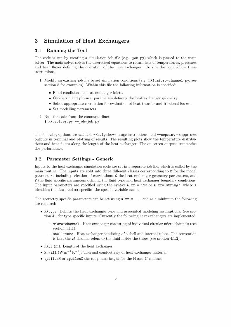
Micro-channel heat exchangers, such as Printed Circuit Heat Exchangers can be modelled byapproximating their geometry to a matrix of parallel tubes as shown in Fig. 3. The microchannels are modelled as circular tubes with separation t1 and t2 respectively. The hot and coldfluid passes through alternating horizontal rows of tubes. To model this type of heat exchangerset G.HXtype = ‘mirco-channel’ and define the following extra variables in the input job file:

• N_T (−): Number of tubes.

• d (m): Internal diameter of tubes

• D (m): External diameter of tubes.

• DD (m): Internal diameter of shell.

• t_casing (m: Thickness of shell.

• d_tube (m: Equivalent diameter of passages.

For the micro channel heat exchanger the derived parameters are calculated as follows:

• Area (m2):

Aeff, 1 = NC (dtube + t2) × (2NR − 1) ×HXL (default) (4.1a)

Aeff, 2 = NC NR dtube πHXL (4.1b)

10

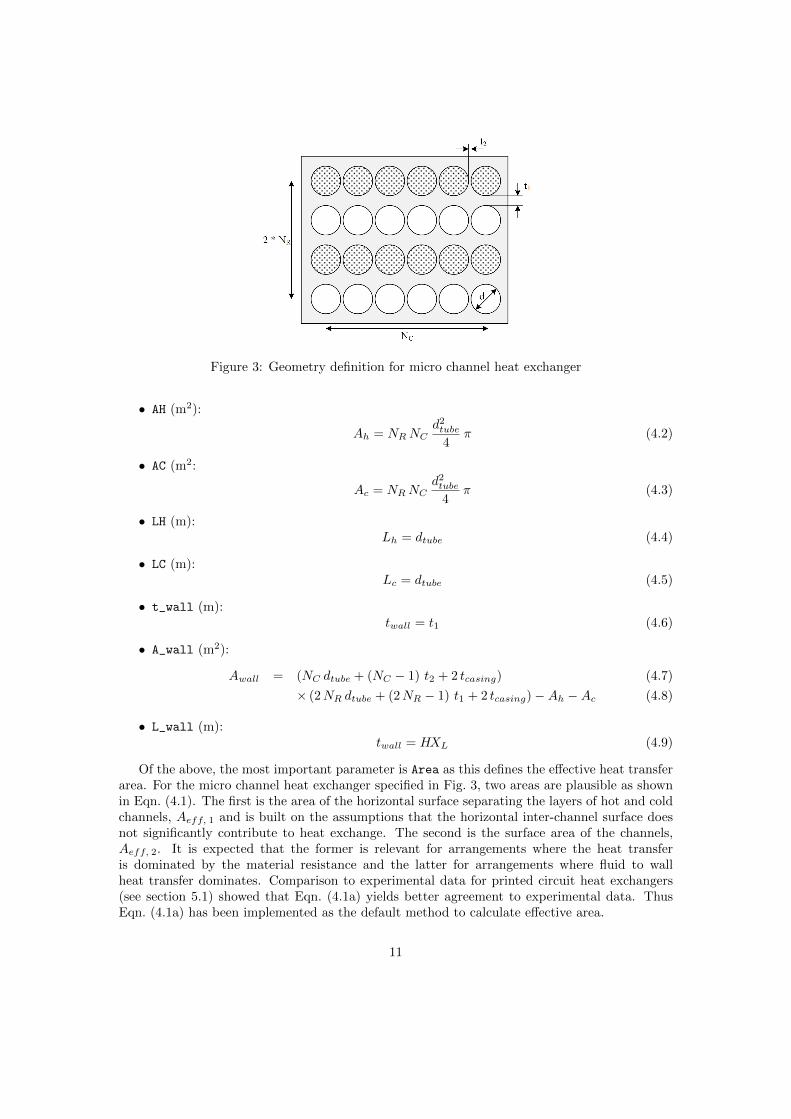
Figure 3: Geometry definition for micro channel heat exchanger

• AH (m2):

Ah = NRNCd2tube

4π (4.2)

• AC (m2:

Ac = NRNCd2tube

4π (4.3)

• LH (m):Lh = dtube (4.4)

• LC (m):Lc = dtube (4.5)

• t_wall (m):twall = t1 (4.6)

• A_wall (m2):

Awall = (NC dtube + (NC − 1) t2 + 2 tcasing) (4.7)

× (2NR dtube + (2NR − 1) t1 + 2 tcasing) −Ah −Ac (4.8)

• L_wall (m):twall = HXL (4.9)

Of the above, the most important parameter is Area as this defines the effective heat transferarea. For the micro channel heat exchanger specified in Fig. 3, two areas are plausible as shownin Eqn. (4.1). The first is the area of the horizontal surface separating the layers of hot and coldchannels, Aeff, 1 and is built on the assumptions that the horizontal inter-channel surface doesnot significantly contribute to heat exchange. The second is the surface area of the channels,Aeff, 2. It is expected that the former is relevant for arrangements where the heat transferis dominated by the material resistance and the latter for arrangements where fluid to wallheat transfer dominates. Comparison to experimental data for printed circuit heat exchangers(see section 5.1) showed that Eqn. (4.1a) yields better agreement to experimental data. ThusEqn. (4.1a) has been implemented as the default method to calculate effective area.

11

Figure 4: Geometry definition for shell and tube heat exchanger

4.1.2 Shell and Tube Heat Exchanger

Shell and tube heat exchangers are a common type of heat exchanger commonly employed. Herea number of small diameter tubes are arranged inside a larger shell as shown in Fig. 4. Withinthis code the convention is that the H channel is inside the tubes and the shell side is the Cchannel. To model this type of heat exchanger set G.HXtype = ‘shell-tube’ and define thefollowing extra variables in the input job file:

• N_T (−): Number of tubes.

• d (m): Internal diameter of tubes

• D (m): External diameter of tubes.

• DD (m): Internal diameter of shell.

• t_casing (m): Thickness of shell.

For the tube and shell heat exchanger the derived parameters are calculated as follows:

• Area (m2):Aeff = d πHXL (4.10)

• AH (m2):

Ah = NTd2tube

4π (4.11)

• AC (m2:

Ac =DD2

4π −NT

d2tube4

π (4.12)

• Lc_H (m):LcH = d (4.13)

• Lc_C (m):LcC = D (4.14)

12

• Dh_H (m):DhH = d (4.15)

• Dh_C (m):

DhC =4Ac

DDπ +NT Dπ(4.16)

• t_wall (m):

twall =D − d

2(4.17)

• A_wall (m2):

Awall = DDπ twall +NTD2 − d2

4π (4.18)

• L_wall (m):Lwall = HXL (4.19)

Of the above the most important parameter is Area as this defines the effective heat transferarea.

4.1.3 New Heat Exchangers

To add new heat exchanger types, the source code and the Geomtry class can be altered. Simplyadd a new class internal function analogous to micro_init. This function must return all thestandard outputs listed at the beginning of this section.

4.2 Implemented Heat Transfer Correlations

Heat transfer is critically determined by empirical heat transfer correlations that take accountof the local flow conditions, thermal properties, buoyancy effects and also geometry. To date thefollowing correlations for Nusselt number, Nu have been implemented. The correlations can beselected by using the corresponding index to set M.Nu_CorrelationH and M.Nu_CorrelationC.The use of different correlations, for example to account for up and downwards flow, is supported.

1. CO2 flow in pipes near the critical point, as developed by Yoon et al. [3]. Correlation hasonly been implemented for Tb > Tpc

Nub = 0.14Re0.69b Pr0.66b (4.20)

b and w refer to bulk and wall properties respectively.

2. CO2 flow in horizontal pipes, as developed by Liao et al. [2].

Nub = 0.124Re0.8b Pr0.4b

(Gr

Re2b

)0.203 (ρwρb

)0.842 (cpcp, b

)0.384

(4.21)

cp =iw − ibTw − Tb

(4.22)

b and w refer to bulk and wall properties respectively.

13

Table 1: Coefficients for air flow across cylinders

Re C n0.0001-0.004 0.437 0.09850.004-0.09 0.565 0.1360.09-1.0 0.800 0.2801-35 0.795 0.38435-5000 0.583 0.4715000-50 000 0.148 0.63350 000 - 200 000 0.0208 0.814

3. CO2 flow in vertical pipes and upwards flow, as developed by Liao et al. [2].

Nub = 0.354Re0.8b Pr0.4b

(GrmRe2.7b

)0.157 (ρwρb

)1.297 (cpcp, b

)0.296

(4.23)

b and w refer to bulk and wall properties respectively.

4. CO2 flow in vertical pipes and downwards flow, as developed by Liao et al. [2].

Nub = 0.643Re0.8b Pr0.4b

(GrmRe2.7b

)0.186 (ρwρb

)2.154 (cpcp, b

)0.751

(4.24)

b and w refer to bulk and wall properties respectively.

5. Fluid flow inside of circular pipes, as developed by Boelter [4].

Nu = 0.23RePrn (4.25)

with

{n = 0.3 for heating of fluidn = 0.4 for cooling of fluid

6. Fluid flow on the shell side of shell and tube heat exchangers, as per the paper by Xie et.al. [7]

Nu = eC+m logRE Pr13 (4.26)

with C = 0.16442; m = 0.65582

7. Tubes in air cross flow with characteristic length equal to tube diameter. For this case twocorrelations are implemented to differentiate between natural and forced convection [5].

Natural Convection: 0 < Re < 0.0001

Nu = C (GrPr)n

(4.27)

with

{for Gr Pr < 1 × 109 C = 0.053; n = 1

4for Gr Pr > 1 × 109 C = 0.126; n = 1

3

Force Convection: Re > 0.0001

Nu = C Re (4.28)

with coefficients listed in Tab. 1.

14

4.2.1 New Heat Transfer Correlations

To add new heat transfer correlations, extend the function calc_Nu and add new Correlationoptions that can be specified. The function must return a local value of Nusselt number.

4.3 Implemented Heat Exchanger Pressure Drop Options

A number of modelling approaches have been implemented to model pressure change along theheat exchanger channels. These can be categorised in two groups. In the first a friction factoris calculated, which allows calculation of the pressure drop based on local condition (changingpressure and temperature) along the respective heat exchanger channel. The friction factor, f isconverted to a pressure drop from one cell to the next using the relationship:

∆P = ρ

(∆L

DHfV 2

2

), (4.29)

where ∆L is the length of a cell, DH is the hydraulic diameter of the channel, and V is thechannel mean velocity.

In the second, pressures are specified at the inlet and outlet of the heat exchanger and alinear pressure drop is assumed within the heat exchanger. The outlet pressure can either bespecified directly by the user, by setting PH_out or PC_out, or alternatively by specifying alist containing coefficients for a pressure drop vs mass flow rate polynomial. When a list ofpolynomial coefficents is defined, the pressure drop and downstream pressure are calculated by:

∆P =

N∑i=1

ai mi, (4.30)

Pout = Pin − ∆P, (4.31)

where ai are the polynomial coefficients defined in the lists H_dP_poly and C_dP_poly for the Hand C channel respectively. When using the polynomial in either channel the friction correlationoption 0 has to be selected and a linear pressure between Pin and Pout is modelled.

The following options have been implemented for the calculation of friction factor f :

1. No friction. The model will either assume a constant pressure if only inlet pressure, Pin issupplied, or apply a linear pressure drop if both inlet and outlet pressure are supplied.

f = 0 (4.32)

2. This option automatically switches between the relationships of correlation 3 and 4 based onchannel Reynolds number. For Re ≤ 2300 correlation 3 is used, for Re > 2300 correlation4 is used.

3. Laminar flow

f =64

Re. (4.33)

4. Turbulent flow using Haaland’s formula

1

f12

= −1.8 log

(( εDH

3.7

)1

.11 +6.9

Re

), (4.34)

where ε is the pipe roughness height.

15

4.3.1 New Friction Factor Correlations

To add new pressure loss correlations the function calc_friction can be extend to include newCorrelation options. The function must return a local value of friction factor, f .

16

Figure 5: Printed Circuit Heat Exchanger (PCHEX) used by VanMeter [6]

Table 2: PCHEX dimensions estimated by Van meter. [6]. ( Items are marked with ∗ the averageof values listed by VanMeter was used)

Parameter Value Parameter ValueNumber of layers - N_CR 21 Number of Columns 53Channel diameter - tube 1.506 mm Average channel length∗ - HX_L 1304 mmPlate thickness - t_1 1.31 mm Thickness between channels - t_2 0.48 mmCasing thickness∗ - t_casing 38.55 mm

5 Examples and Validation

The following examples illustrate the usage of the code and also act to demonstrate the validity

5.1 Micro Channel Heat Exchanger

Printed Circuit Heat Exchangers (PCHEX) are a type of micro-channel heat exchanger. Thechemically bonded plates with engraved channels are an efficient way to create effective andcompact heat exchangers. However, the compactness can also lead to notable losses due to con-duction within the heat exchanger’s metallic structure. Furthermore the high thermal gradientscause high mechanical stresses and increase thermal losses.

For the demonstration of the micro-channel heat exchanger model the experimental workby VanMeter [6] was selected. As a first step his work estimates the internal structure of thePCHEX shown in Fig. 5. The data converted to HX_solver.py input parameters is summarisedin Tab. 2 and the corresponding simulation set-up file is:

1 ”””2 Example case based on the sCO2 heat exchanger s tudy by :3 Josh Van Meter (2006) Experimental I n v e s t i g a t i o n o f a Printed Ci r cu i t Heat4 Exchanger us ing Su p e r c r i t i c a l Carbon Dioxide and Water as Heat Transfer Media ,5MsC Thesis , Kansas S ta te Un ive r i s t y6

7 Used fo r v a l i d a t i o n o f the micro channel heat exchanger model and fo r8 v e r i f i c a t i o n fo r s u p e r c r i t i c a l f l u i d s imua l t i ons .9

10 Author : Ingo Jahn11 Last : Modif ied 23/03/201712 ”””13

14# se t f l u i d cond i t i ons at heat exchanger i n l e t and o u t l e t15 F. f lu idH = ’CO2 ’16 F. TH in = 273.15+88.17 F.mdotH = 100./3600

17

Table 3: Cell number sensitivity study for case with mCO2 = 300 kg/h and CO2 outlet temper-ature at 36 ◦C.

N_cell HTC (W m−1 K−1) % difference N_cell HTC (W m−1 K−1) % difference5 236.30 28.7 10 186.38 1.520 0.31 0 40 183.69 0.07100 183.57 [n/a]

18 F. PH in = 8 . e619 F. f lu idC = ’ water ’20 F. TC in = 273.15+36.021 F.mdotC = 700./360022 F. PC in = 1 . e523 F. T ext = 295 # Externa l Temperature (K) op t i ona l24

25 F.T0 = [ ]26

27# se t geometry f o r heat exhanger − requ i red s e t t i n g s depend on type28G.HXtype = ’micro−channel ’29G.N R = 21 # number o f rows in HX30G.N C = 53 # number o f columns in HX matrix31G. t 1 = 1.31 e−3 #32G. t 2 = 0.48 e−3 #33G. t c a s i n g = 0 . 5∗ ( 4 4 . 6 e−3 + 32 .5 e−3) #34G.HX L = 0.5∗ ( 1 . 230 + 1 .378 ) # leng t h o f HX (m)35G. d tube = 1.506 e−3 # tube diameter36G. k wa l l = 16 # thermal c onduc t i v i t y (W / m /K)37G. eps i lonH = 0 . # roughness h e i g h t f o r H channel38G. eps i lonC = 0 . # roughness h e i g h t f o r C cahannel39

40# Set mode l l ing parameters41M. N ce l l = 40 # number o f c e l l s42M. f l a g a x i a l = 143M. e x t e r n a l l o s s = 044M. Nu CorrelationH = 245M. Nu Correlat ionC = 546M. f Cor r e l a t i onH = 147M. co f l ow = 0

To obtain solution independence a sensitivity study on cell number was performed and theresults are shown in Tab. 3. This shows that 20 or more cells are required in order to obtainaccurate results.

Temperature, pressure and energy flux distributions within the heat exchanger are shown inFig. 6. These show that significant heat transfer takes place close to the hot CO2 inlet side, andthat heat transfer diminishes closer to the CO2 outlet. This effect is driven by the nonlinearproperties of CO2 close to the critical point (304.25 K, 7.39 MPa), which also create a pinchpoint within the heat exchanger. To validate the simulation results the predicted heat transfercoefficient for the current test case: CO2 inlet conditions 88 ◦C, 8 MPa, 300 kg/h and CO2 outlettemperature 36 ◦C are compared to the corresponding experimental data from Van Meter [6] inFig. 6d. Two sets of simulation results are shown corresponding to effective area being calculatedwith Eqns. (4.1a & b). This graphs shows reasonable agreement between the experimental dataand predictions. Using the tube surface area (A1-case) consistently under-predicts the heattransfer coefficient. Using the area of the separating surface (A2-case) shows better agreement,however the gradient is somewhat over-predicted. This suggests that the implemented Nusseltnumber correlations do not fully capture the heat transfer enhancement of the micro channels.

18

(a) Temperature (b) Energy Flow

(c) Pressure Distribution(d) Comparison to heat transfer coefficient datafrom Van Meter

Figure 6: Solutions for heat exchanger preoperties for case with mCO2 = 300 kg/h and CO2

outlet temperature of 36 ◦C .

19

Future work should investigate the use of more accurate heat transfer correlations.

20

5.2 Shell and Tube Heat Exchanger

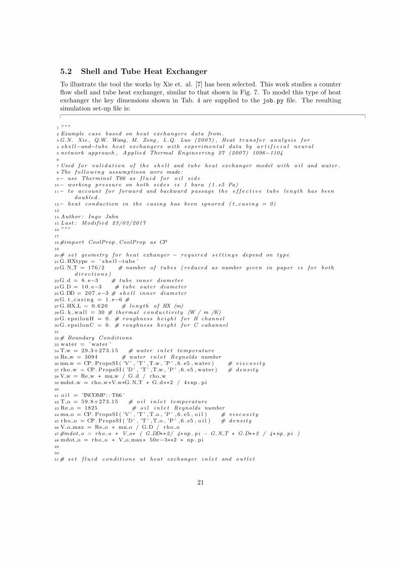
To illustrate the tool the works by Xie et. al. [7] has been selected. This work studies a counterflow shell and tube heat exchanger, similar to that shown in Fig. 7. To model this type of heatexchanger the key dimensions shown in Tab. 4 are supplied to the job.py file. The resultingsimulation set-up file is:

1 ”””2 Example case based on heat exchangers data from .3G.N. Xie , Q.W. Wang, M. Zeng , L .Q. Luo (2007) , Heat t r an s f e r ana l y s i s f o r4 s h e l l−and−tube heat exchangers with exper imenta l data by a r t i f i c i a l neura l5 network approach , Appl ied Thermal Engineering 27 (2007) 1096−11046

7 Used fo r v a l i d a t i o n o f the s h e l l and tube heat exchanger model wi th o i l and water .8 The f o l l ow i n g assumptiosn were made :9− use Therminol T66 as f l u i d f o r o i l s i d e

10− working pressure on both s i d e s i s 1 bara (1 . e5 Pa)11− to account f o r forward and backward passage the e f f e c t i v e tube l eng t h has been

doub led .12− heat conduction in the cas ing has been ignored ( t c a s i n g = 0)13

14 Author : Ingo Jahn15 Last : Modif ied 23/03/201716 ”””17

18#import CoolProp . CoolProp as CP19

20# se t geometry f o r heat exhanger − requ i red s e t t i n g s depend on type21G.HXtype = ’ s h e l l−tube ’22G.N T = 176/2 # number o f tubes ( reduced as number g iven in paper i s f o r both

d i r e c t i o n s )23G. d = 8 . e−3 # tube inner diameter24G.D = 10 . e−3 # tube outer diameter25G.DD = 207 . e−3 # s h e l l inner diameter26G. t c a s i n g = 1 . e−6 #27G.HX L = 0.620 # leng t h o f HX (m)28G. k wa l l = 30 # thermal c onduc t i v i t y (W / m /K)29G. eps i lonH = 0 . # roughness h e i g h t f o r H channel30G. eps i lonC = 0 . # roughness h e i g h t f o r C cahannel31

32# Boundary Condit ions33 water = ’ water ’34 T w = 29.3+273.15 # water i n l e t temperature35 Re w = 3094 # water i n l e t Reynolds number36 mu w = CP. PropsSI ( ’V ’ , ’T ’ ,T w , ’P ’ , 6 . e5 , water ) # v i s c o s i t y37 rho w = CP. PropsSI ( ’D ’ , ’T ’ ,T w , ’P ’ , 6 . e5 , water ) # dens i t y38 V w = Re w ∗ mu w / G. d / rho w39 mdot w = rho w∗V w∗G.N T ∗ G. d∗∗2 / 4∗np . p i40

41 o i l = ’INCOMP: : T66 ’42 T o = 59.8+273.15 # o i l i n l e t temperature43 Re o = 1825 # o i l i n l e t Reynolds number44 mu o = CP. PropsSI ( ’V ’ , ’T ’ ,T o , ’P ’ , 6 . e5 , o i l ) # v i s c o s i t y45 rho o = CP. PropsSI ( ’D ’ , ’T ’ ,T o , ’P ’ , 6 . e5 , o i l ) # dens i t y46 V o max = Re o ∗ mu o / G.D / rho o47#mdot o = rho o ∗ V o∗ ( G.DD∗∗2/ 4∗np . p i − G.N T ∗ G.D∗∗2 / 4∗np . p i )48 mdot o = rho o ∗ V o max∗ 50e−3∗∗2 ∗ np . p i49

50

51# se t f l u i d cond i t i ons at heat exchanger i n l e t and o u t l e t

21

Figure 7: Shell and tube heat exchanger used by Xie et. al. [7]

Table 4: Shell and tube heat exchanger dimensions from Xie et al. [7]. Estimated items aremarked with ∗

Parameter Value Parameter ValueNumber of tubes 176 Effective length of tubes 620 mmTube outer diameter 10 mm Tube inner diameter 8 mmInner diameter of shell 207 mm

52 F. f lu idH = ’ water ’53 F. TH in = T w54 F. PH in = 6 . e555 F. PH out = 6 . e556 F.mdotH = mdot w57 F. f lu idC = o i l58 F. TC in = T o59 F.mdotC = 5 .60 F. PC in = 6 . e561 F. PC out = 6 . e562 F.mdotC = mdot o63 F.T0 = [ ]64

65 print ”Masslfows : mdot o i l=” ,F .mdotC , ’ ; mdot water=’ ,F .mdotH , ’ ( kg/ s ) ’66

67# Set mode l l ing parameters68M. N ce l l = 10# number o f c e l l s69M. f l a g a x i a l = 170M. e x t e r n a l l o s s = 071M. Nu CorrelationH = 572M. Nu Correlat ionC = 673M. f Cor r e l a t i onH = 074M. co f l ow = 0

The boundary conditions and corresponding results for the 10 cases presented by Xie et al.are shown in Tab. 5. Table 6 shows the results from a cell number (N_cell) independencystudy, which shows that results become grid independent once more than 20 cells are used.The corresponding detailed results for test case (1) are shown in Fig. 8. These plots show thetemperature profiles with respect to normalised position along the heat exchanger and also theinternal heat fluxes corresponding to Fig. 8b.

The results are within the range presented by Xie et al. [7], confirming the correct imple-mentation of the model and also it’s suitability to analyse heat exchangers. Discrepancies to theactual results are expected to be caused by the use of an incorrect heat transfer oil, as the actualfluid type was not provided by the authors.

22

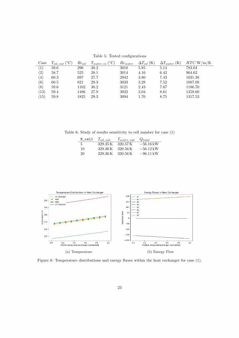
Table 5: Tested configurations

Case Toil, out (◦C) Reoil Twater, in (◦C) Rewater ∆Toil (K) ∆Twater (K) HTC W/m/K(1) 59.6 296 30.2 3010 5.85 5.14 783.04(2) 58.7 525 28.1 3014 4.16 6.42 964.62(4) 60.3 697 27.7 2942 3.80 7.43 1031.38(6) 60.5 821 29.3 3033 3.28 7.52 1087.08(8) 59.6 1102 30.2 3121 2.43 7.67 1186.70(13) 59.4 1486 27.9 3022 2.04 8.61 1258.60(15) 59.8 1825 29.3 3094 1.70 8.75 1317.53

Table 6: Study of results sensitivity to cell number for case (1)

N_cell Toil, out Twater, out Qtotal5 329.35 K 320.57 K −56.16 kW10 329.36 K 320.56 K −56.12 kW20 329.36 K 320.56 K −96.11 kW

(a) Temperature (b) Energy Flow

Figure 8: Temperature distributions and energy fluxes within the heat exchanger for case (1).

23

6 References

References

[1] I. H. Bell, J. Wronski, S. Quoilin, V. Lemort, 2014, Pure and Pseudo-pure Fluid Thermophys-ical Property Evaluation and the Open-Source Thermophysical Property Library CoolProp, In-dustrial & Engineering Chemistry Research, 53(6):2498–2508, 2014. doi:10.1021/ie4033999.

[2] S.M. Liao, T.S. Zhao, 2002, An experimental investigation of convection heat transfer to su-percritical carbon dioxide in miniature tubes, International Journal of Heat and Mass Transfer,45, (2002), 50255034

[3] S. H. Yoon, J. H. Kim, Y. W. Hwang, M. S. Kim, K. Min, Y. Kim, 2003, Heat transferand pressure drop characteristics during the in-tube cooling process of carbon dioxide in thesupercritical region, International Journal of Refrigeration, 26, (2003), 857864

[4] F. O. Incropera, D. P. DeWitt 2007, Fundamentals of Heat and Mass Transfer, New York:Wiley, ISBN 978-0-471-45728-2

[5] A. M. Howatson, P. G. Lund, J. D. Todd 1991, Engineering Tables and data, London: Chap-man & Hall

[6] J. Van Meter, 2006, Experimental Investigation of a Printed Circuit Heat Exchanger usingSupercritical Carbon Dioxide and Water as the Heat Transfer Media, Master of Science Thesis,Kansas State University, USA

[7] G. N. Xie, Q. W. Wang, M. Zeng, L. Q. Luo, 2007, Heat transfer analysis for shell-and-tube heat exchangers with experimental data by artificial neural network approach, AppliedThermal Engineering, 27, (2007), 1096-1104

7 Appendix

7.1 Example Input file job example.py

1 ”””2 Template input f i l e f o r HX solver . py3 ”””4

5# se t f l u i d cond i t i ons at heat exchanger i n l e t and o u t l e t6 F. f lu idH = ’CO2 ’7 F. TH in = 756.1704490658 F.mdotH = 5 .9 F. PH in = 7.68 e6

10 F. PH out = 7.68 e611 F. TC in = 324.9148100212 F.mdotC = 5 .13 F. PC in = 12 . e614 F. PC out = 12 . e615 F. T ext = 295 # Externa l Temperature (K) op t i ona l16

17 F.T0 = [ ]18

24

19# se t geometry f o r heat exhanger − requ i red s e t t i n g s depend on type20G.HXtype = ’micro−channel ’21G.N R = 100 # number o f rows in HX22G.N C = 400 # number o f columns in HX matrix23G. t 1 = 2e−3 #24G. t 2 = 0 .5 e−3 #25G. t c a s i n g = 5e−3 #26G.HX L = 1 . # leng t h o f HX (m)27G. d tube = 1 .5 e−3 # tube diameter28G. k wa l l = 16 # thermal c onduc t i v i t y (W / m /K)29G. eps i lonH = 0 . # roughness h e i g h t f o r H channel30G. eps i lonC = 0 . # roughness h e i g h t f o r C cahannel31

32# Set mode l l ing parameters33M. N ce l l = 10 # number o f c e l l s34M. f l a g a x i a l = 135M. e x t e r n a l l o s s = 036M. Nu CorrelationH = 237M. Nu Correlat ionC = 238M. f Cor r e l a t i onH = 139M. co f l ow = 0

7.2 Source Code HX solver.py

1#! /usr / bin /env python2 ”””3 Python Code to eva lua t e on− and o f f−des ign performance o f heat exchangers .4

5 Function has two oepra t ing modes :6 (1) Stand alone7 This e va l ua t e s the heat exchanger performance and can be used to p l o t8 temperature t r a ce s i n s i d e the heat exchanger .9

10 (2) imported11 The func t ion i s can be c a l l e d by Cycle . py to a l l ow the quasi−s teady eva lua t i on12 o f heat exchanger performance as par t o f Cycle o f f−des ign mode l l ing .13

14 Version : 1.015 Author : Ingo Jahn16 Last Modif ied : 26/03/201717 ”””18

19 import numpy as np20 import CoolProp . CoolProp as CP21 import s c ipy as s c i22 from s c ipy import opt imize23 import matp lo t l i b . pyplot as p l t24 import sys as sys25 import os as os26 from getopt import getopt27

28###29###30 class Fluid :31 def i n i t ( s e l f ) :32 s e l f . f lu idH = [ ]33 s e l f . f l u idC = [ ]34 s e l f . TH in = [ ] # (K)

25

35 s e l f .mdotH = [ ] # ( kg/s )36 s e l f . PH in = [ ] # pressure (Pa)37 s e l f . PH out = [ ] # pressure (Pa)38 s e l f . TC in = [ ] # (K)39 s e l f .mdotC = [ ] # ( kg/s )40 s e l f . PC in = [ ] # pressure (Pa)41 s e l f . PC out = [ ] # pressure (Pa)42 s e l f . T ext = [ ] # ambient surroundign temperature43 s e l f . T0 = [ ]44 ###45 def check ( s e l f ,M) :46 i f not s e l f . f lu idH and not s e l f . f l u idC :47 raise MyError ( ’ Ne i ther F . f lu idH or F . f lu idC s p e c i f i e d ’ )48 i f s e l f . f lu idH and not s e l f . f l u idC :49 s e l f . f l u idC = s e l f . f lu idH50 print ’ f l u idC not s p e c i f i e d and s e t to equal f lu idH ’51 i f s e l f . f l u idC and not s e l f . f lu idH :52 s e l f . f lu idH = s e l f . f l u idC53 print ’ f lu idH not s p e c i f i e d and s e t to equal f lu idC ’54 i f not s e l f . TH in :55 raise MyError ( ’F . TH in not s p e c i f i e d c o r r e c t l y ’ )56 i f not s e l f .mdotH :57 raise MyError ( ’F . mdot H not s p e c i f i e d ’ )58 i f not s e l f . PH in :59 raise MyError ( ’F . PH in not s p e c i f i e d ’ )60 i f not s e l f . PH out :61 s e l f . PH out = s e l f . PH in62 print ’ PH out not s p e c i f i e d and s e t to equal PH in ’63 i f not s e l f . TC in :64 raise MyError ( ’F . TC in not s p e c i f i e d ’ )65 i f not s e l f .mdotC :66 s e l f .mdotC = s e l f .mdotH67 print ’mdotC not s p e c i f i e d and s e t to equal mdotH ’68 i f s e l f .mdotC < 0 . or s e l f .mdotH < 0 . :69 raise MyError ( ’Mass f low r a t e s in both channe l s needs to be > 0 . ’ )70 i f not s e l f . PC in :71 raise MyError ( ’F . PC in not s p e c i f i e d ’ )72 i f not s e l f . PC out :73 s e l f . PC out = s e l f . PC in74 print ’ PC out not s p e c i f i e d and s e t to equal PC in ’75 #i f M. e x t e r n a l l o s s i s 1 :76 # i f not s e l f . T ext :77 # ra i s e MyError ( ’ T ext not s p e c i f i e d ’)78 #79 i f M. p r i n t f l a g :80 print ’ Check o f Fluid input parameters : Passed ’81

82 ###83 def get T0 ( s e l f ,M) :84 ”””85 f unc t i on to s e t i n i t i a l / o ld cond i t i ons86 ”””87 i f len ( s e l f . T0) i s 0 :88 T0 = np . z e r o s ( (4∗M. N ce l l ) )89

90

91 # se t TWH92 T0 [M. N c e l l : 2∗M. N ce l l ] = np . ones (M. N c e l l ) ∗ 0 . 5∗ ( s e l f . TH in+s e l f .

TC in )93 # se t TWC94 T0[2∗M. N ce l l : 3∗M. N ce l l ] = np . ones (M. N c e l l ) ∗ 0 . 5∗ ( s e l f . TH in+s e l f .

TC in )

26

95 i f M. co f l ow :96 # se t TH97 T0 [ 0 :M. N c e l l ] = s e l f . TH in + np . arange (M. N c e l l ) / f loat (M. N c e l l )

∗( s e l f . TC in−s e l f . TH in ) ∗0 .2598 # se t TC99 T0[3∗M. N ce l l : 4∗M. N ce l l ] = s e l f . TC in − np . arange (M. N c e l l ) / f loat

(M. N c e l l ) ∗( s e l f . TC in−s e l f . TH in ) ∗0 .25100 else :101 # se t TH102 T0 [ 0 :M. N c e l l ] = s e l f . TH in + np . arange (M. N c e l l ) / f loat (M. N c e l l )

∗( s e l f . TC in−s e l f . TH in ) ∗0 .5103 # se t TC104 T0[3∗M. N ce l l : 4∗M. N ce l l ] = s e l f . TC in − (1.−np . arange (M. N c e l l ) /

f loat (M. N c e l l ) ) ∗( s e l f . TC in−s e l f . TH in ) ∗0 .5105 #T0[4∗M. N ce l l :5∗M. N ce l l ] = np . ones (M. N ce l l ) ∗ 0.5∗ ( s e l f . PH in

+ s e l f . PH out )106 #T0[5∗M. N ce l l :6∗M. N ce l l ] = np . ones (M. N ce l l ) ∗ 0.5∗ ( s e l f . PC in +

s e l f . PC out )107 return T0108 else :109 return s e l f . T0110###111###112 class Model :113 def i n i t ( s e l f ) :114 s e l f . optim =’ root : hybr ’115 s e l f . N c e l l = [ ] # number o f c e l l s116 s e l f . c o f l ow = 0 # de f a u l t i s to ana lyse counter f l ow heat exchangers . Set

to 1 fo r co f l ow117 s e l f . f l a g a x i a l = [ ] # whether a x i a l heat conduct ion i s cons idered118 s e l f . e x t e r n a l l o s s = [ ] # whether e x t e rna l heat l o s s i s cons idered119 s e l f . Nu CorrelationH = [ ] # se t c o r r e l a t i on fo r heat t r an s f e r in H channel120 s e l f . Nu Correlat ionC = [ ] # se t c o r r e l a t i on fo r heat t r an s f e r in C channel121 s e l f . f Co r r e l a t i onH = [ ] # se t c o r r e l a t i on fo r f r i c t i o n f a c t o r in H

channel122 s e l f . f Co r r e l a t i onC = [ ] # se t c o r r e l a t i on fo r f r i c t i o n f a c t o r in C

channel123 s e l f . H dP poly = [ ] # polynominal c o e f f i c i e n t s f o r pressure drop in H

channel124 s e l f . C dP poly = [ ] # polynominal c o e f f i c i e n t s f o r pressure drop in H

channel125 ###126 def check ( s e l f ) :127 i f not s e l f . N c e l l :128 raise MyError ( ’M. N c e l l not s p e c i f i e d ’ )129 i f not s e l f . f l a g a x i a l :130 s e l f . f l a g a x i a l = 0131 print ’M. f l a g a x i a l no s p e c i f i e d d e f au l t i n g to 0 ’132 i f not s e l f . Nu CorrelationH :133 raise MyError ( ’M. Nu CorrelationH not s p e c i f i e d ’ )134 i f not s e l f . Nu Correlat ionC :135 s e l f . Nu Correlat ionC = s e l f . Nu CorrelationH136 print ’ Nu Correlat ionC not s p e c i f i e d and s e t to equal Nu CorrelationH ’137 i f not isinstance ( s e l f . f Cor re la t i onH , int ) :138 raise MyError ( ’M. f Cor r e l a t i onH not s p e c i f i e d ’ )139 i f not isinstance ( s e l f . f Cor re l a t i onC , int ) :140 s e l f . f Co r r e l a t i onC = s e l f . f Co r r e l a t i onH141 print ’ f Co r r e l a t i onC not s p e c i f i e d and s e t to equal f Co r r e l a t i onH ’142 i f not ( s e l f . c o f l ow == 0 or s e l f . c o f l ow == 1) :143 raise MyError ( ’M. co f l ow not de f ined c o r r e c t l y . Set to 0 or 1 ’ )144 i f len ( s e l f . H dP poly ) > 0 and s e l f . f Co r r e l a t i onH != 0 :

27

145 raise MyError ( ’ Pres sure drop polynominal H dP poly can only be used incon junct ion with f Cor r e l a t i onH = 0 ’ )

146 i f len ( s e l f . C dP poly ) > 0 and s e l f . f Co r r e l a t i onC != 0 :147 raise MyError ( ’ Pres sure drop polynominal C dP poly can only be used in

con junct ion with f Co r r e l a t i onC = 0 ’ )148 #149 i f s e l f . p r i n t f l a g :150 print ’ Check o f Model input parameters : Passed ’151###152###153 def s e t p o l y ( s e l f ,F) :154 # use polynominal to update o u t l e t pressure155 i f len ( s e l f . H dP poly ) > 0 :156 temp = [ ]157 for a in range ( len ( s e l f . H dP poly ) ) :158 temp . append ( s e l f . H dP poly∗F.mdotC∗∗a )159 F. PC out = sum( temp)160

161 i f len ( s e l f . C dP poly ) > 0 : # i f polynominal i s s p e c i f i e d use t h i s to ca l cPH out

162 temp = [ ]163 for a in range ( len ( s e l f . C dP poly ) ) :164 temp . append ( s e l f . C dP poly∗F.mdotC∗∗a )165 F. PC out = sum( temp)166###167###168 class Geometry :169 def i n i t ( s e l f ) :170 s e l f . HXtype = [ ]171 s e l f . k wa l l = [ ] # thermal c onduc t i v i t y (W / mk)172 s e l f . t y p e l i s t = [ ’ micro−channel ’ , ’ s h e l l−tube ’ ]173 ###174 def c h e c k i n i t i a l i s e ( s e l f ,M) :175 i f not s e l f . HXtype :176 raise MyError ( ’G. HXtype not s p e c i f i e d ’ )177 i f not any( s e l f . HXtype in s for s in s e l f . t y p e l i s t ) :178 raise MyError ( ’ S p e c i f i e d type in G. HXtype not supported . Use : ’+s e l f .

t y p e l i s t )179

180 # look at microchannel case181 i f s e l f . HXtype == ’micro−channel ’ :182 s e l f . micro check ( )183 s e l f . m i c r o i n i t ( )184 #185 i f s e l f . HXtype == ’ sh e l l−tube ’ :186 s e l f . s h e l l t ub e ch e c k ( )187 s e l f . s h e l l t u b e i n i t ( )188 #189 i f M. p r i n t f l a g :190 print ’ Check o f Geometry input parameterrs : Passed ’191 ###192 def micro check ( s e l f ) :193 i f not s e l f .N R :194 raise MyError ( ’G.N R not s p e c i f i e d ’ )195 i f not s e l f .N C :196 raise MyError ( ’G.N C not s p e c i f i e d ’ )197 i f not s e l f . t 1 :198 raise MyError ( ’G. t 1 not s p e c i f i e d ’ )199 i f not s e l f . t 2 :200 raise MyError ( ’G. t 2 not s p e c i f i e d ’ )201 i f not s e l f . t c a s i n g :202 raise MyError ( ’G. t c a s i n g not s p e c i f i e d ’ )

28

203 i f not s e l f .HX L :204 raise MyError ( ’G.HX L not s p e c i f i e d ’ )205 i f not s e l f . d tube :206 raise MyError ( ’G. d tube not s p e c i f i e d ’ )207 i f not s e l f . k wa l l :208 raise MyError ( ’G. k wa l l not s p e c i f i e d ’ )209 ###210 def mi c r o i n i t ( s e l f ) :211 s e l f . Area = s e l f .N C ∗ ( s e l f . d tube + s e l f . t 2 ) ∗ (2∗ s e l f .N R−1) ∗ s e l f .

HX L212 #s e l f . Area = s e l f .N C ∗ s e l f .N R ∗ ( s e l f . d tube ∗ np . p i ) ∗ s e l f .HX L213

214 s e l f .AH = s e l f .N R∗ s e l f .N C ∗ s e l f . d tube ∗∗2/4 ∗np . p i # t o t a l f l ow area (m2)

215 s e l f . Lc H = s e l f . d tube # cha r a c t e r i s t i c l en g t h (m)216 s e l f .Dh H = s e l f . d tube217 s e l f .AC = s e l f .N R∗ s e l f .N C ∗ s e l f . d tube ∗∗2/4 ∗np . p i # t o t a l f l ow area (

m2)218 s e l f . Lc C = s e l f . d tube # cha r a c t e r i s t i c l en g t h (m)219 s e l f . Dh C = s e l f . d tube220

221 s e l f . t wa l l = s e l f . t 1 # (m)222

223 L1 = s e l f .N C∗ s e l f . d tube + ( s e l f .N C−1)∗ s e l f . t 2 + 2∗ s e l f . t c a s i n g224 L2 = 2∗ s e l f .N R∗ s e l f . d tube+ (2∗ s e l f .N R−1)∗ s e l f . t 1 + 2∗ s e l f . t c a s i n g225 s e l f . A wall = L1∗L2 − s e l f .AH − s e l f .AC226

227 s e l f . L wal l = s e l f .HX L228 ###229 def s h e l l t ub e ch e c k ( s e l f ) :230 i f not s e l f .N T :231 raise MyError ( ’G.N T not s p e c i f i e d ’ )232 i f not s e l f . d :233 raise MyError ( ’G. d not s p e c i f i e d ’ )234 i f not s e l f .D:235 raise MyError ( ’G.D not s p e c i f i e d ’ )236 i f not s e l f .DD:237 raise MyError ( ’G.DD not s p e c i f i e d ’ )238 i f not s e l f . t c a s i n g :239 raise MyError ( ’G. t c a s i n g not s p e c i f i e d ’ )240 i f not s e l f .HX L :241 raise MyError ( ’G.HX L not s p e c i f i e d ’ )242 i f not s e l f . k wa l l :243 raise MyError ( ’G. k wa l l not s p e c i f i e d ’ )244 ###245 def s h e l l t u b e i n i t ( s e l f ) :246 s e l f . Area = 0 . 5∗ ( s e l f . d +s e l f .D) ∗ np . p i ∗ s e l f .HX L ∗ s e l f .N T247 s e l f .AH = s e l f .N T ∗ s e l f . d∗∗2/4 ∗np . p i # t o t a l f l ow area (m2)248 s e l f . Lc H = s e l f . d # cha r a c t e r i s t i c l en g t h (m)249 s e l f .Dh H = s e l f . d # hydrau l i c diameter250 s e l f .AC = s e l f .DD∗∗2/4∗np . p i − s e l f .N T∗ s e l f .D∗∗2/4.∗np . p i # t o t a l f l ow

area (m2)251 s e l f .AC = s e l f .AC252 s e l f . Lc C = s e l f .D # cha r a c t e r i s t i c l en g t h (m)253 Perimeter = s e l f .DD ∗ np . p i + s e l f .N T ∗ s e l f .D∗np . p i254 s e l f . Dh C = 4.∗ s e l f .AC / Perimeter # hydrau l i c diameter255

256 s e l f . t wa l l = ( s e l f .D−s e l f . d ) /2 . # (m)257

258 s e l f . A wall = s e l f .DD∗np . p i ∗ s e l f . t wa l l + s e l f .N T ∗ ( s e l f .D∗∗2 − s e l f . d∗∗2) / 4 .∗np . p i

259

29

260 s e l f . L wal l = s e l f .HX L261##262##263 def calc Nu (P,Tm,Tp,Tw, mdot , A tota l , L c , f l u i d , Co r r e l a t i on ) :264 ”””265 f unc t i on to c a l c u l a t e l o c a l Nusse l t number based on bu l k f l ow p rop e r t i e s266 Inputs :267 P − bu l k pressure (Pa)268 Tm − bu l k temperature to l e f t (K)269 Tp − bu l k temperature to r i g h t (K)270 Tw − temperature o f wa l l (K)271 mdot − t o t a l mass f l ow ra te ( kg/s )272 A to ta l − t o t a l f l ow area (m∗∗2)273 L c − c h a r a c t e r i s t i c l en g t h (m)274 f l u i d − f l u i d type275 Corre la t ion − s e l e c t c o r r e l a t i o n to be used :276 1 − Yoon co r r e l a t i on fo r sCO2 in p ipes f o r Tb > Tpc277 2 − S .M. Liao and T. S Zhaou co r r e l a t i on fo r micorchannels278 h t t p ://www.me. us t . hk/˜mezhao/ pdf /33.PDF279 − ho r i z on t a l p ipes280 3 − S .M. Liao and T. S Zhaou co r r e l a t i on fo r micorchannels281 h t t p ://www.me. us t . hk/˜mezhao/ pdf /33.PDF282 − v e r t i c a l pipes , upwards f l ow283 4 − − S .M. Liao and T. S Zhaou co r r e l a t i on fo r micorchannels284 h t t p ://www.me. us t . hk/˜mezhao/ pdf /33.PDF285 − v e r t i c a l pipes , downwards f l ow286

287 Outputs :288 Nu − Nussel Number289 ”””290 Tb = 0 .5∗ (Tm+Tp) # bu l k temperature291

292 # ca l c u l a t e Prandl number293 Pr = CP. PropsSI ( ’PRANDTL’ , ’P ’ ,P, ’T ’ , Tb , f l u i d )294

295 # c l a c u l a t e Reynolds number296 rho b = CP. PropsSI ( ’DMASS’ , ’P ’ ,P, ’T ’ , Tb , f l u i d )297 U = abs ( mdot / ( rho b ∗ A tota l ) )298 mu b = CP. PropsSI ( ’VISCOSITY ’ , ’P ’ ,P, ’T ’ , Tb , f l u i d )299 Re = rho b ∗ U ∗ L c / mu b300

301 i f Cor r e l a t i on i s 1 :302 # Yoon co r r e l a t i on fo r ho r i z on t a l p ipes303 Nu = 0.14 ∗ Re∗∗0 .69 ∗ Pr ∗∗0 .66304 e l i f Cor r e l a t i on i s 2 :305 # Liao co r r e l a t i on fo r ho r i z on t a l p ipes306 rho w = CP. PropsSI ( ’DMASS’ , ’P ’ ,P, ’T ’ , Tw , f l u i d )307 Gr = abs ( 9 .80665 ∗ ( rho b−rho w ) ∗ rho b ∗L c ∗∗3 / mu b∗∗2)308 Cp b = CP. PropsSI ( ’CPMASS ’ , ’P ’ ,P, ’T ’ , Tb , f l u i d )309 i b = CP. PropsSI ( ’UMASS’ , ’P ’ ,P, ’T ’ , Tb , f l u i d )310 i w = CP. PropsSI ( ’UMASS’ , ’P ’ ,P, ’T ’ , Tw , f l u i d )311 i f Tw == Tb:312 Nu = 0 .313 else :314 Cp bar = ( i w−i b ) / (Tw−Tb)315 #pr in t ’Gr : ’ , Gr , ’ Cp bar : ’ , Cp bar316 Nu = 0.124 ∗ Re∗∗0 .8 ∗ Pr ∗∗0 .4 ∗ (Gr/Re∗∗2) ∗∗0.203 ∗ ( rho w/ rho b )

∗∗0.842 ∗ ( Cp bar / Cp b ) ∗∗0.384317 e l i f Cor r e l a t i on i s 3 :318 # Liao co r r e l a t i on fo r v e r t i c a l p ipes − upwards f l ow319 rho w = CP. PropsSI ( ’DMASS’ , ’P ’ ,P, ’T ’ , Tw , f l u i d )320 rho mid = CP. PropsSI ( ’DMASS’ , ’P ’ ,P, ’T ’ , 0 . 5∗ (Tw+Tb) , f l u i d )

30

321 rho m = 1/(Tw−Tb) ∗ (Tw−Tb) /6 . ∗ ( rho b + 4∗ rho mid + rho w ) #in t e g r a t i on us ing Simpsons ru l e

322 Gr m = abs ( 9 .80665 ∗ ( rho b−rho m ) ∗ rho b ∗L c ∗∗3 / mu b∗∗2)323 Cp b = CP. PropsSI ( ’CPMASS ’ , ’P ’ ,P, ’T ’ , Tb , f l u i d )324 i b = CP. PropsSI ( ’UMASS’ , ’P ’ ,P, ’T ’ , Tb , f l u i d )325 i w = CP. PropsSI ( ’UMASS’ , ’P ’ ,P, ’T ’ , Tw , f l u i d )326 i f Tw == Tb:327 Nu = 0 .328 else :329 Cp bar = ( i w−i b ) / (Tw−Tb)330 #pr in t ’Gr : ’ , Gr , ’ Cp bar : ’ , Cp bar331 Nu = 0.354 ∗ Re∗∗0 .8 ∗ Pr ∗∗0 .4 ∗ (Gr m/Re∗∗2 .7 ) ∗∗0.157 ∗ ( rho w/ rho b )

∗∗1.297 ∗ ( Cp bar / Cp b ) ∗∗0.296332 e l i f Cor r e l a t i on i s 4 :333 # Liao co r r e l a t i on fo r v e r t i c a l p ipes − downwards f l ow334 rho w = CP. PropsSI ( ’DMASS’ , ’P ’ ,P, ’T ’ , Tw , f l u i d )335 rho mid = CP. PropsSI ( ’DMASS’ , ’P ’ ,P, ’T ’ , 0 . 5∗ (Tw+Tb) , f l u i d )336 rho m = 1/(Tw−Tb) ∗ (Tw−Tb) /6 . ∗ ( rho b + 4∗ rho mid + rho w ) #

in t e g r a t i on us ing Simpsons ru l e337 Gr m = abs ( 9 .80665 ∗ ( rho b−rho m ) ∗ rho b ∗L c ∗∗3 / mu b∗∗2)338 Cp b = CP. PropsSI ( ’CPMASS ’ , ’P ’ ,P, ’T ’ , Tb , f l u i d )339 i b = CP. PropsSI ( ’UMASS’ , ’P ’ ,P, ’T ’ , Tb , f l u i d )340 i w = CP. PropsSI ( ’UMASS’ , ’P ’ ,P, ’T ’ , Tw , f l u i d )341 i f Tw == Tb:342 Nu = 0 .343 else :344 Cp bar = ( i w−i b ) / (Tw−Tb)345 #pr in t ’Gr : ’ , Gr , ’ Cp bar : ’ , Cp bar346 Nu = 0.643 ∗ Re∗∗0 .8 ∗ Pr ∗∗0 .4 ∗ (Gr m/Re∗∗2 .7 ) ∗∗0.186 ∗ ( rho w/ rho b )

∗∗2.154 ∗ ( Cp bar / Cp b ) ∗∗0.751347 e l i f Cor r e l a t i on i s 5 :348 # For f l ow in c i r c u l a r p ipes ( from HLT) use f o r incompres s i b l e f l u i d s (

water/ o i l )349 # Dit tus Boe l t e r Equation350 i f Tw > Tb: # heat ing o f f l u i d351 n = 0 .3352 else : # coo l ing o f f l u i d353 n = 0 .4354 Nu = 0.023 ∗ Re∗∗0 .8 ∗ Pr∗∗n355 e l i f Cor r e l a t i on i s 6 :356 # Corre la t ion fo r s h a e l l s i d e as per paper by Xie e t a l .357 C = 0 .16442 ; m=0.65582358 e = np . exp ( C + m ∗ np . l og (Re) )359 Nu = e ∗ Pr ∗ ∗ ( 1 . / 3 . )360 e l i f Cor r e l a t i on i s 7 :361 i f Re == 0 . or Re < 0 . 0 001 :362 # use Natural Convection r e l a t i o n s h i p363 rho w = CP. PropsSI ( ’DMASS’ , ’P ’ ,P, ’T ’ , Tw , f l u i d )364 beta = 1 ./Tb365 Gr = abs ( 9 .80665 ∗ rho w ∗∗2 ∗ L c ∗∗3 ∗ (Tw − Tb) ∗ beta / mu b∗∗2)366 GrPr = Gr∗Pr367 i f GrPr <= 1e9 :368 C = 0 . 5 3 ; n=1/4369 else :370 C = 0 . 1 2 6 ; n=1/3371 Nu = C ∗ GrPr ∗∗n372 i f Re > 0 .0001 and Re <= 0 . 0 0 4 :373 C = 0 . 4 3 7 ; n = 0.0985374 e l i f Re >0.004 and Re <= 0 . 0 9 :375 C = 0 . 5 6 5 ; n = 0.136376 e l i f Re > 0 .09 and Re <= 1 . :377 C = 0 . 8 ; n = 0.280

31

378 e l i f Re > 1 .0 and Re <= 35 . :379 C = 0 . 7 9 5 ; n= 0.384380 e l i f Re > 35 . and Re <= 5000 . :381 C = 0 . 5 8 3 ; n = 0.471382 e l i f Re > 5000 . and Re <= 50000 . :383 C = 0 . 1 4 8 ; n = 0.633384 e l i f Re > 50000 . and Re <= 200000:385 C = 0 . 0208 ; n = 0.814386 else :387 raise MyError ( ’ Co r r e l a t i on out s id e range o f va l i d Nusse l t numbers . ’ )388

389 else :390 raise MyError ( ’ Co r r e l a t i on opt ion f o r Nusse l t number c a l c u l a t i o n not

implemented . ’ )391

392 return Nu393##394##395 def c a l c f r i c t i o n (P, Tm, Tp, mdot , A tota l , Dh, f l u i d , Cor re la t i on , e p s i l o n = 0 . ) :396 ”””397 f unc t i on to c a l c u l a t e l o c a l f r i c t i o n f a c t o r based on l o c a l geometry and bu l k

f l ow p rop e r t i e s398 Inputs :399 P − bu l k pressure (Pa)400 Tm − bu l k temperature to l e f t (K)401 Tp − bu l k temperature to r i g h t (K)402 mdot − t o t a l mass f l ow ra te ( kg/s )403 A to ta l − t o t a l f l ow area (m∗∗2)404 Dh − Hydraul ic Diameter (m)405 f l u i d − f l u i d type406 Corre la t ion − s e l e c t c o r r e l a t i o n to be used :407 1 − au tma t i c a l l y sw i t che s between laminar and t u r bu l en t f l ow408 2 − laminar f l ow − c i r c u l a r p ipe409 3 − t u r bu l en t f l ow − rough p ipes (Haaland ’ s formula )410 ep s i l on − roughness h e i gh t (m)411

412 Outputs :413 f − f r i c t i o n f a c t o r414 ”””415 Tb = 0 .5∗ (Tm+Tp) # bu l k temperature416

417 # c l a c u l a t e Reynolds number418 rho b = CP. PropsSI ( ’DMASS’ , ’P ’ ,P, ’T ’ , Tb , f l u i d )419 U = abs (mdot / ( rho b ∗ A tota l ) )420 mu b = CP. PropsSI ( ’VISCOSITY ’ , ’P ’ ,P, ’T ’ , Tb , f l u i d )421 Re = rho b ∗ U ∗ Dh / mu b422 i f Cor r e l a t i on i s 1 :423 i f Re < 2300 :424 f = 64 . / Re425 else :426 temp = np . log10 ( ( e p s i l o n /Dh / 3 . 7 ) ∗1 .11 + (6 . 9/Re ) )427 f = (−1.8 ∗ temp ) ∗∗−2.428 e l i f Cor r e l a t i on i s 2 :429 # laminar pipe f l ow430 f = 64 . / Re431 e l i f Cor r e l a t i on i s 3 :432 # tubu l en t rough p ipes433 temp = np . log10 ( ( e p s i l o n /Dh / 3 . 7 ) ∗1 .11 + (6 . 9/Re ) )434 f = (−1.8 ∗ temp ) ∗∗−2.435

436 else :

32

437 raise MyError ( ’ Co r r e l a t i on opt ion f o r f r i c t i o n f a c t o r c a l c u l a t i o n notimplemented . ’ )

438

439 # pr in t Gr / Re∗∗2440

441 return f442###443###444 def equat ions (T, M, G, F , f l a g =0) :445 ”””446 f unc t i on tha t e va l ua t e s the s teady s t a t e energy ba lance f o r each c e l l447 Inputs :448 T − vec to r conta ing temperatures and pres sure s at var ious i n t e r f a c e po in t s449 M − c l a s s conta in ign model parameters450 G − c l a s s conta in ing geometry parameters451 F − c l a s s conta in ing f l u i d boundary cond i t i ons452 f l a g − a l l ows opera t ion fo func t i on to be a l t e r e d453 0 − d e f a u l t f o r opera t ion454 1 − output temperature and heat f l u x e s455 2 − re turns pressure t r ac e s456 Outputs :457 error − vec to r conta in ing miss−ba lance in energy equa t ions f o r d i f f e r e n t

l c o a t i on s458 ”””459 TH, TWH, TWC, TC= open T (T,F . TH in ,F . TC in ,F . PH in ,F . PC in ,M,F)460

461 # pr in t ’ Temperature ’ ,TH,TWH,TC462 i f f l a g i s 1 :463 Q1 = [ ] ; Q2 = [ ] ; Q3 = [ ]464 Q4 = [ ] ; Q5 = [ ] ; Q6 = [ ]465 Q7 = [ ] ; Q8 = [ ]466

467 e r r o r = np . z e r o s (4∗M. N ce l l )468

469 # ca l c u l a t e Pressure d i s t r i b u t i o n in both p ipes based on current temperatures470 # pressure i s c a l c u l a t e d in f l ow d i r e c t i on .471 PH = [F . PH in ] ; PC=[F . PC in ]472 for i in range (M. N c e l l ) :473 i f M. f Cor r e l a t i onH == 0 : # apply l i n e a r pressure drop i f no c o r r e l a t i on

i s s p e c i f i c e d474 PH. append (F . PH in − (F . PH in − F. PH out ) / (M. N ce l l −1.) ∗ ( i +1) )475 e l i f M. f Cor r e l a t i onH == 1 :476 # ca l c u l a t e pressure drop due to f r i c t i o n477 f= c a l c f r i c t i o n (PH[ i −1] ,TH[ i ] ,TH[ i +1] ,F .mdotH ,G.AH,G.Dh H , F . f lu idH ,

M. f Corre la t i onH , G. eps i lonH )478 rhoH = CP. PropsSI ( ’D ’ , ’P ’ , PH[ i −1] , ’T ’ , TH[ i ] ,F . f lu idH )479 V = F.mdotH / rhoH / G.AH # ca l c u l a t e f l ow v e l o c i t y480 h f = f ∗ G.HX L/(M. N c e l l +1.) /G.Dh H ∗ V∗V / ( 2 . ∗ 9 . 8 1 ) # ca l c u l a t e

f r i c t i o n head l o s s481 dP = h f ∗ rhoH ∗ 9 .81482 PH. append (PH[ i ] − dP)483 else :484 raise MyError ( ’ Core l a t i on type not implemented ’ )485

486 i f M. f Cor r e l a t i onC == 0 : # apply l i n e a r pressure drop i f no c o r r e l a t i oni s s p e c i f i c e d

487 PC. append (F . PC in − (F . PC in − F. PC out ) / (M. N ce l l −1.) ∗ ( i +1) )488 e l i f M. f Cor r e l a t i onC == 1 :489 i f M. co f l ow :490 f= c a l c f r i c t i o n (PC[ i −1] ,TC[ i ] ,TC[ i +1] ,F .mdotC ,G.AC,G.Dh C , F .

f lu idC , M. f Cor re l a t i onC , G. eps i lonC )491 rhoC = CP. PropsSI ( ’D ’ , ’P ’ , PC[ i −1] , ’T ’ , TC[ i ] ,F . f lu idC )

33

492 V = F.mdotC / rhoC / G.AC # ca l c u l a t e f l ow v e l o c i t y493 h f = f ∗ G.HX L/(M. N c e l l +1.) /G.Dh C ∗ V∗V / ( 2 . ∗ 9 . 8 1 ) #

ca l c u l a t e f r i c t i o n head l o s s494 dP = h f ∗ rhoC ∗ 9 .81495 PC. append (PC[ i ] − dP)496 else :497 # ca l c u l a t e pressure drop due to f r i c t i o n498 j = M. N c e l l − i − 1 #499 f= c a l c f r i c t i o n (PC[ i −1] ,TC[ j ] ,TC[ j +1] ,F .mdotC ,G.AC,G.Dh C , F .

f lu idC , M. f Cor re l a t i onC , G. eps i lonC )500 rhoC = CP. PropsSI ( ’D ’ , ’P ’ , PC[ i −1] , ’T ’ , TC[ j ] ,F . f l u idC )501 V = F.mdotC / rhoC / G.AC # ca l c u l a t e f l ow v e l o c i t y502 h f = f ∗ G.HX L/(M. N c e l l +1.) /G.Dh C ∗ V∗V / ( 2 . ∗ 9 . 8 1 ) #

ca l c u l a t e f r i c t i o n head l o s s503 dP = h f ∗ rhoC ∗ 9 .81504 PC. append (PC[ i ] − dP)505 else :506 raise MyError ( ’ Core l a t i on type not implemented ’ )507

508

509 i f not M. co f l ow : #510 # rever se d i r e c t i on o f PC as f l ow i s from i = −1 to i = 0511 PC = l i s t ( reversed (PC) )512

513 #pr in t ’PH ’ , PH514 #pr in t ’PC ’ , PC515

516 # ca l c u l a t e energy ba lance f o r h igh pressure stream (H) ; low pressure stream (C) and d i v i d i n g wa l l

517 for i in range (M. N c e l l ) :518

519 #pr in t ’ In HX solver ’520 #pr in t ’TH’ , TH521 #pr in t ’PH ’ , PH522 kH = CP. PropsSI ( ’CONDUCTIVITY’ , ’P ’ , ( 0 . 5∗ (PH[ i ]+PH[ i +1]) ) , ’T ’ , ( 0 . 5∗ (TH[ i

]+TH[ i +1]) ) ,F . f lu idH )523 kHm = CP. PropsSI ( ’CONDUCTIVITY’ , ’P ’ , PH[ i ] , ’T ’ , TH[ i ] ,F .

f lu idH )524 kHp = CP. PropsSI ( ’CONDUCTIVITY’ , ’P ’ , PH[+1 ] , ’T ’ , TH[ i +1] ,F

. f lu idH )525 kC = CP. PropsSI ( ’CONDUCTIVITY’ , ’P ’ , ( 0 . 5∗ (PC[ i ]+PC[ i +1]) ) , ’T ’ , ( 0 . 5∗ (TC[ i

]+TC[ i +1]) ) ,F . f lu idC )526 kCm = CP. PropsSI ( ’CONDUCTIVITY’ , ’P ’ , PC[ i ] , ’T ’ , TC[ i ] ,F .

f l u idC )527 kCp = CP. PropsSI ( ’CONDUCTIVITY’ , ’P ’ , PC[ i +1] , ’T ’ , TC[ i +1] ,F

. f lu idC )528

529 NuH = calc Nu ( ( 0 . 5 ∗ (PH[ i ]+PH[ i +1]) ) ,TH[ i ] ,TH[ i +1] ,TWH[ i ] , F .mdotH , G.AH, G. Lc H , F . f lu idH , M. Nu CorrelationH )

530 NuC = calc Nu ( ( 0 . 5 ∗ (PC[ i ]+PC[ i +1]) ) ,TC[ i ] ,TC[ i +1] ,TWC[ i ] , F .mdotC , G.AC, G. Lc C , F . f lu idC , M. Nu Correlat ionC )

531

532 hH = NuH ∗ kH / G. Lc H533 hC = NuC ∗ kC / G. Lc C534

535 # heat t r a sn f e r in H channel536 q1 conv = CP. PropsSI ( ’HMASS’ , ’P ’ ,PH[ i ] , ’T ’ ,TH[ i ] ,F . f lu idH ) ∗ F.mdotH537 i f i == 0 :538 q1 cond = − kHm ∗ G.AH/ (G. L wal l /M. N c e l l / 2 . ) ∗ ( 0 . 5∗ (TH[ i ] + TH[ i

+1]) − TH[ i ] )539 else :

34

540 q1 cond = − kHm ∗ G.AH/ (G. L wal l /M. N c e l l ) ∗ ( 0 . 5∗ (TH[ i ] + TH[ i+1]) − 0 . 5∗ (TH[ i ] + TH[ i −1]) )

541 q1 = q1 conv + q1 cond542

543 q2 conv = CP. PropsSI ( ’HMASS’ , ’P ’ ,PH[ i +1] , ’T ’ ,TH[ i +1] ,F . f lu idH ) ∗ F.mdotH544 i f i == M. N ce l l −1:545 q2 cond = − kHp ∗ G.AH/ (G. L wal l /M. N c e l l / 2 . ) ∗ ( TH[ i +1]

− 0 . 5∗ (TH[ i ] + TH[ i +1]) )546 else :547 q2 cond = − kHp ∗ G.AH/ (G. L wal l /M. N c e l l ) ∗ ( 0 . 5∗ (TH[ i +1] + TH[ i

+2]) − 0 . 5∗ (TH[ i ] + TH[ i +1]) )548 q2 = q2 conv + q2 cond549 q3 = hH ∗ G. Area/M. N c e l l ∗ ( 0 . 5∗ (TH[ i ]+TH[ i +1]) − TWH[ i ] )550

551 # Heat Transfer in wa l l552 q7 temp = (G. k wa l l ∗ G. Area/M. N c e l l ) /G. t wa l l ∗ (TWH[ i ] − TWC[ i ] )553 i f M. f l a g a x i a l i s 1 :554 i f i == 0 :555 q7 p = − G. k wa l l ∗ G. A wall / (G. L wal l /M. N c e l l ) ∗ ( 0 . 5∗ (TWH[ i

+1]+TWC[ i +1]) − 0 . 5∗ (TWH[ i ] +TWC[ i ] ) )556 q7 m = 0 .557 e l i f i == M. N ce l l −1:558 q7 p = 0 .559 q7 m = − G. k wa l l ∗ G. A wall / (G. L wal l /M. N c e l l ) ∗ ( 0 . 5∗ (TWH[ i ]

+TWC[ i ] ) − 0 . 5∗ (TWH[ i−1]+TWC[ i −1]) )560 else :561 q7 p = − G. k wa l l ∗ G. A wall / (G. L wal l /M. N c e l l ) ∗ ( 0 . 5∗ (TWH[ i

+1]+TWC[ i +1]) − 0 . 5∗ (TWH[ i ] +TWC[ i ] ) )562 q7 m = − G. k wa l l ∗ G. A wall / (G. L wal l /M. N c e l l ) ∗ ( 0 . 5∗ (TWH[ i ]

+TWC[ i ] ) − 0 . 5∗ (TWH[ i−1]+TWC[ i −1]) )563 else :564 q7 p = 0 .565 q7 m = 0 .566 q7h = q7 temp − 0 .5 ∗ (−q7 p +q7 m)567 q7c = q7 temp + 0 .5 ∗ (−q7 p +q7 m)568

569 q4 = hC ∗ G. Area/M. N c e l l ∗ (TWC[ i ] − 0 . 5∗ (TC[ i ]+TC[ i +1]) )570 qC cond = − kC ∗ G.AC/ (G. L wal l /M. N c e l l ) ∗ ( TC[ i +1] − TC[ i ] )571

572 # Heat Transfer in C Channel573 q5 conv = CP. PropsSI ( ’HMASS’ , ’P ’ ,PC[ i ] , ’T ’ ,TC[ i ] ,F . f l u idC ) ∗ −F.mdotC574 i f i == 0 :575 q5 cond = − kCm ∗ G.AC/ (G. L wal l /M. N c e l l / 2 . ) ∗ ( 0 . 5∗ (TC[ i ] + TC[ i

+1]) − TC[ i ] )576 else :577 q5 cond = − kCm ∗ G.AC/ (G. L wal l /M. N c e l l ) ∗ ( 0 . 5∗ (TC[ i ] + TC[ i

+1]) − 0 . 5∗ (TC[ i ] + TC[ i −1]) )578 q5 = q5 conv + q5 cond579 q6 conv = CP. PropsSI ( ’HMASS’ , ’P ’ ,PC[ i +1] , ’T ’ ,TC[ i +1] ,F . f lu idC ) ∗ −F.mdotC580 i f i == M. N ce l l −1:581 q6 cond = − kCp ∗ G.AC/ (G. L wal l /M. N c e l l / 2 . ) ∗ ( TC[ i +1]

− 0 . 5∗ (TC[ i ] + TC[ i +1]) )582 else :583 q6 cond = − kCp ∗ G.AC/ (G. L wal l /M. N c e l l ) ∗ ( 0 . 5∗ (TC[ i +1] + TC[ i

+2]) − 0 . 5∗ (TC[ i ] + TC[ i +1]) )584 q6 = q6 conv + q6 cond585

586 # ca l c u l a t e mis−match in energy f l u x e s587 #pr in t q1 , q2 , q3588 e r r o r [ i ] = q1−q2−q3589 e r r o r [M. N c e l l+i ] = q3−q7h590 e r r o r [ 2∗M. N ce l l+i ] = q4−q7c

35

591 e r r o r [ 3∗M. N ce l l+i ] = q4+q5−q6592

593 i f f l a g i s 1 :594 Q1. append ( q1 ) ; Q2 . append ( q2 ) ; Q3 . append ( q3 )595 Q4. append ( q4 ) ; Q5 . append ( q5 ) ; Q6 . append ( q6 )596 Q7. append ( q7h ) ; Q8 . append ( q7c )597

598 #pr in t q1 , q2 , q3 , q4 , q5 , q6 , q7599 #pr in t ’ Error ’ , error600 #pr in t i601

602 i f f l a g i s 0 :603 return e r r o r604 e l i f f l a g i s 1 :605 return e r ror , T, Q1, Q2, Q3, Q4, Q5, Q6, Q7, Q8606 e l i f f l a g i s 2 :607 return PH, PC608 else :609 raise MyError ( ’ f l a g opt ion not de f ined . ’ )610###611###612 def open T (T, TH in , TC in , PH in , PC in ,M,F) :613 ”””614 f unc t i on to unpack the Temperature vec to r T in to the 6 vec t o r s615 TH, TWH, TWC, TC, PH, PC616 ”””617 N ce l l = M. N c e l l618

619 TH = np . z e r o s ( N c e l l +1)620 TWH = np . z e r o s ( N c e l l )621 TWC = np . z e r o s ( N c e l l )622 TC = np . z e r o s ( N c e l l +1)623 TH[ 0 ] = TH in624 TH[ 1 : N c e l l +2] = T[ 0 : N c e l l ]625 TWH = T[ N c e l l : 2∗ N ce l l ]626 TWC = T[2∗ N ce l l : 3∗ N ce l l ]627 i f M. co f l ow :628 TC[ 0 ] = TC in629 TC[ 1 : N c e l l +2] = T[3∗ N ce l l : 4∗ N ce l l ]630 else :631 TC[ 0 : N c e l l ] = T[3∗ N ce l l : 4∗ N ce l l ]632 TC[ N c e l l ] =TC in633

634

635

636 return TH,TWH,TWC,TC #,PH,PC637###638###639 def main ( uoDict ) :640 ”””641 main func t ion642 ”””643 # crea te s t r i n g to c o l l e c t warning messages644 warn st r = ”\n”645

646 # main f i l e to be executed647 jobFileName = uoDict . get ( ”−−job ” , ” t e s t ” )648

649 # s t r i p . py ex t ens ion form jobName650 jobName = jobFileName . s p l i t ( ’ . ’ )651 jobName = jobName [ 0 ]652

36

653 # crea te c l a s s e s to s t o r e input data654 M = Model ( )655 F = Fluid ( )656 G = Geometry ( )657

658 # se t p r i n t f l a g ( can be overwr i t t en from j o b f i l e )659 M. p r i n t f l a g = 1660 i f uoDict . has key ( ”−−nopr int ” ) :661 M. p r i n t f l a g = 0662

663 # Execute j obF i l e , t h i s c r ea t e s a l l the v a r i a b l e s664 execf i le ( jobFileName , globals ( ) , locals ( ) )665

666 i f M. p r i n t f l a g :667 print ” Input data f i l e read ”668

669 # Check t ha t requ i red input data has been prov ided670 M. check ( )671 F. check (M)672 M. s e t p o l y (F)673 G. c h e c k i n i t i a l i s e (M)674

675 # I n i t i a l i s e temperature vec to r676 T0 = F. get T0 (M)677

678 # change f l ow d i r e c t i on o f co ld channel i f co f l ow679 i f M. co f l ow :680 F.mdotC = −F.mdotC681

682 # pr in t ’T0 ’ , T0683

684 # se t up t up l e o f op t i ona l inpu t s f o r use by f s o l v e685 args = (M, G, F , 0)686

687 i f M. optim == ’ f s o l v e ’ :688 T , i n f od i c t , s tatus , mesg = s c i . opt imize . f s o l v e ( equat ions ,T0 , args=args ,

f u l l o u t pu t =1)689 e l i f M. optim == ’ root : hybr ’ :690 s o l = s c i . opt imize . root ( equat ions ,T0 , args=args , method=’ hybr ’ , opt ions={ ’

x t o l ’ : 1 . e−12})691 s t a tu s = s o l . s t a tu s692 T = so l . x693 mesg = s o l . message694 e l i f gdata . optim == ’ root : lm ’ :695 s o l = s c i . opt imize . root ( equat ions ,A0 , args=args , method=’ lm ’ , opt i ons={ ’ eps ’

: 1 . e−3, ’ x t o l ’ : 1 . e−12, ’ f t o l ’ : 1 e−12})696 s t a tu s = s o l . s t a tu s697 A = so l . x698 mesg = s o l . message699 e l i f gdata . optim == ’ root : Newton−CG’ :700 s o l = s c i . opt imize . root ( equat ions ,A0 , args=args , method=’ lm ’ , opt i ons={ ’ eps ’

: 1 . e−3, ’ x t o l ’ : 1 . e−12})701 s t a tu s = s o l . s t a tu s702 A = so l . x703 mesg = s o l . message704 e l i f gdata . optim == ’ root : df−sane ’ :705 s o l = s c i . opt imize . root ( equat ions ,A0 , args=args , method=’ df−sane ’ , opt ions={ ’

f t o l ’ : 1 . e−12})706 s t a tu s = s o l . s t a tu s707 A = so l . x708 mesg = s o l . message709 else :

37

710 raise MyError ( ”gdata . optim = ’ ’ not s e t p reope r ly . ” )711

712 i f s t a tu s i s not 1 :713 print mesg714 raise MyError ( ’ HX solver . py : f s o l v e unable to converge . ’ )715

716 TH, TWH, TWC, TC = open T (T,F . TH in ,F . TC in ,F . PH in ,F . PC in ,M,F)717 # open T(T,F. TH in ,F. TC in ,M. N ce l l )718

719 # crea te pressure t r a c e s f o r output720 PH, PC= equat ions (T, M, G, F , 2)721

722 i f M. p r i n t f l a g :723 print ” P lo t t i ng r e s u l t s ”724 plot HX (TH,TWH,TWC,TC,M. N c e l l )725 e r ror , T, Q1, Q2, Q3, Q4, Q5, Q6, Q7, Q8= equat ions (T, M, G, F , 1)726 plot HXq (Q1, Q2, Q3, Q4, Q5, Q6, Q7, Q8, M. N ce l l , G.HX L)727 plot Hp (PH,PC,M. N c e l l )728

729 #pr in t Q1, ’\n ’ , Q2, ’\n ’ , Q3, ’\n ’ , Q4, ’\n ’ , Q5, ’\n ’ , Q6, ’\n ’ , Q7 , ’\n ’ , Q8

730

731 print ”\n”732 print ’ Temperatures : ’733 print ’Hot−channel ’ , TH734 print ’Hot−channel wa l l temp ’ , TWH735 print ’ Cold−channel wa l l temp ’ , TWC736 print ’ Cold−channel ’ , TC737 print ’ \n ’738 print ’ P re s su re s : ’739 print ’Hot−channel ’ , PH740 print ’ Cold−channel ’ , PC741

742 print ”\n \n”743 print ”Power Trans f e r red − (H) channel ”744 print ’ T in (K) : %.2 f ’ %(TH[ 0 ] )745 print ’ T out (K) : %.2 f ’ %(TH[−1])746 print ’ Delta T (K) : %.2 f ’ %(abs (TH[0]−TH[−1]) )747 P inH = CP. PropsSI ( ’HMASS’ , ’P ’ ,F . PH in , ’T ’ ,TH[ 0 ] , F . f lu idH ) ∗ F.mdotH748 P outH = CP. PropsSI ( ’HMASS’ , ’P ’ ,F . PH out , ’T ’ ,TH[−1] ,F . f lu idH ) ∗ F.mdotH749 rho in = CP. PropsSI ( ’D ’ , ’P ’ ,F . PH in , ’T ’ ,TH[ 0 ] , F . f lu idH )750 rho out = CP. PropsSI ( ’D ’ , ’P ’ ,F . PH out , ’T ’ ,TH[−1] ,F . f lu idH )751 mu in = CP. PropsSI ( ’V ’ , ’P ’ ,F . PH in , ’T ’ ,TH[ 0 ] , F . f lu idH )752 mu out = CP. PropsSI ( ’V ’ , ’P ’ ,F . PH out , ’T ’ ,TH[−1] ,F . f lu idH )753 print ’ Power (kW) : %.2 f ’ %((P inH − P outH ) /1 e3 )754 print ’ Reynolds number ( in ) : %.2 f ’ %( rho in ∗F.mdotH/G.AH/ rho in ∗ G.

Lc H / mu in )755 print ’ Reynolds number ( out ) : %.2 f ’ %( rho out ∗F.mdotH/G.AH/ rho out ∗ G.

Lc H / mu out )756 print ”\n”757 print ”Power Trans f e r red − (C) channel ”758 print ’ T in (K) : %.2 f ’ %(TC[−1])759 print ’ T out (K) : %.2 f ’ %(TC[ 0 ] )760 print ’ Delta T (K) : %.2 f ’ %(abs (TC[0]−TC[−1]) )761 P inC = CP. PropsSI ( ’HMASS’ , ’P ’ ,F . PC in , ’T ’ ,TC[ 0 ] , F . f lu idC ) ∗ F.mdotC762 P outC = CP. PropsSI ( ’HMASS’ , ’P ’ ,F . PC out , ’T ’ ,TC[−1] ,F . f lu idC ) ∗ F.mdotC763 rho in = CP. PropsSI ( ’D ’ , ’P ’ ,F . PC in , ’T ’ ,TC[ 0 ] , F . f lu idC )764 rho out = CP. PropsSI ( ’D ’ , ’P ’ ,F . PC out , ’T ’ ,TC[−1] ,F . f lu idC )765 mu in = CP. PropsSI ( ’V ’ , ’P ’ ,F . PC in , ’T ’ ,TC[ 0 ] , F . f lu idC )766 mu out = CP. PropsSI ( ’V ’ , ’P ’ ,F . PC out , ’T ’ ,TC[−1] ,F . f lu idC )767 print ’ Power (kW) : %.2 f ’ %((P inC − P outC ) /1 e3 )

38

768 print ’ Reynolds number ( in ) : %.2 f ’ %( rho in ∗F.mdotC/G.AC/ rho in ∗ G.Lc C / mu in )

769 print ’ Reynolds number ( out ) : %.2 f ’ %( rho out ∗F.mdotC/G.AC/ rho out ∗ G.Lc C / mu out )

770 print ”\n \n”771

772 print ’ Heat Trans fe r In f o : ’773 DT A = TH[ 0 ] − TC[ 0 ] ; DT B = TH[−1] − TC[−1]774 T LM = (DT B − DT A) / np . l og (DT B/DT A)775 #T LM = abs ( ( (TH[−1]−TC[ 0 ] ) − (TH[0]−TC[−1]) ) / (np . l o g ( (TH[−1]−TC[ 0 ] ) /(

TH[0]−TC[−1]) ) ) )776 print ’ Delta T Log Mean (K) : %.2 f ’ %( T LM )777 print ’HTC (W /(m K) : %.2 f ’ %( abs ( P inC − P outC ) / G. Area / abs (T LM) )778

779 print ”\n \n”780 p l t . draw ( )781

782

783 p l t . pause (1 ) # <−−−−−−−784 print ’ \n \n ’785 raw input ( ”<Hit Enter To Close Figures>” )786 p l t . c l o s e ( )787

788 PH out = PH[−1]789 PC out = PC[ 0 ]790 TH out = TH[−1]791 TC out = TC[ 0 ]792

793 return PH out , TH out , PC out , TC out , PH, TH, PC, TC, T0794###795###796 def plot HX (TH,TWH,TWC,TC, N c e l l ) :797 f i g = p l t . f i g u r e ( )798 p l t . p l o t (np . l i n s p a c e ( 0 , 1 . ,num=N ce l l +1) ,TH, ’−− ’ , l a b e l=” (H) Channel” )799 p l t . p l o t (np . l i n s p a c e ( 0 . 5/ N ce l l ,1 . −0 .5/ N ce l l ,num=N ce l l ) ,TWH, ’ o−− ’ , l a b e l=”

Wall” )800 p l t . p l o t (np . l i n s p a c e ( 0 . 5/ N ce l l ,1 . −0 .5/ N ce l l ,num=N ce l l ) ,TWC, ’ o− ’ , l a b e l=”Wall

” )801 p l t . p l o t (np . l i n s p a c e ( 0 , 1 . ,num=N ce l l +1) ,TC, l a b e l = ” (C) Channel” )802 p l t . y l ab e l ( ’ Temperature (K) ’ )803 p l t . x l ab e l ( ’ Po s i t i on along Heat Exchanger ( normal i sed ) ’ )804 p l t . t i t l e ( ’ Temperature D i s t r i bu t i on s in Heat Exchanger ’ )805 p l t . l egend ( l o c=2)806###807###808 def plot Hp (PH,PC, N c e l l ) :809 f i g , ax1 = p l t . subp lo t s ( )810 l 1 = ax1 . p l o t (np . l i n s p a c e ( 0 , 1 . ,num=N ce l l +1) ,PH, ’−− ’ , l a b e l=”Pressure (H)

Channel” )811 ax2 = ax1 . twinx ( )812 l 2 = ax2 . p l o t (np . l i n s p a c e ( 0 , 1 . ,num=N ce l l +1) ,PC, l a b e l = ”Pressure (C) Channel

” )813 ax1 . s e t y l a b e l ( ’ Pres sure H channel (Pa) ’ )814 ax2 . s e t y l a b e l ( ’ Pres sure C channel (Pa) ’ )815 p l t . x l ab e l ( ’ Po s i t i on along Heat Exchanger ( normal i sed ) ’ )816 p l t . t i t l e ( ’ Pres sure D i s t r i bu t i o n s in Heat Exchanger ’ )817 l i n e s = l1+l2818 l a b e l s = [ l . g e t l a b e l ( ) for l in l i n e s ]819 p l t . l egend ( l i n e s , l ab e l s , l o c=2)820

821###822###

39

823 def plot HXq (Q1, Q2, Q3, Q4, Q5, Q6, Q7, Q8, N ce l l , Length ) :824 f i g = p l t . f i g u r e ( )825 p l t . p l o t (np . l i n s p a c e ( 0 , 1 . ,num=N ce l l +1) [0 : −1 ] , np . array (Q1) /1 . e3 ,

l a b e l=”q1” )826 p l t . p l o t (np . l i n s p a c e ( 0 , 1 . ,num=N ce l l +1) [ 1 : ] , np . array (Q2) /1 . e3 ,

l a b e l=”q2” )827 p l t . p l o t (np . l i n s p a c e ( 0 . 5/ N ce l l ,1 . −0 .5/ N ce l l ,num=N ce l l ) , np . array (Q3) /1 . e3 ,

l a b e l=”q3” )828 p l t . p l o t (np . l i n s p a c e ( 0 . 5/ N ce l l ,1 . −0 .5/ N ce l l ,num=N ce l l ) , np . array (Q4) /1 . e3 ,

l a b e l=”q4” )829 p l t . p l o t (np . l i n s p a c e ( 0 , 1 . ,num=N ce l l +1) [0 : −1 ] , np . array (Q5) /1 . e3 ,

l a b e l=”q5” )830 p l t . p l o t (np . l i n s p a c e ( 0 , 1 . ,num=N ce l l +1) [ 1 : ] , np . array (Q6) /1 . e3 ,

l a b e l=”q6” )831 p l t . p l o t (np . l i n s p a c e ( 0 . 5/ N ce l l ,1 . −0 .5/ N ce l l ,num=N ce l l ) , np . array (Q7) /1 . e3 ,

l a b e l=”q7” )832 p l t . p l o t (np . l i n s p a c e ( 0 . 5/ N ce l l ,1 . −0 .5/ N ce l l ,num=N ce l l ) , np . array (Q8) /1 . e3 ,

l a b e l=”q8” )833 p l t . y l ab e l ( ’ Heat Flow (kW) ’ )834 p l t . x l ab e l ( ’ Po s i t i on along Heat Exchanger ( normal i sed ) ’ )835 p l t . t i t l e ( ’ Energy Fluxes in Heat Exchanger ’ )836 p l t . l egend ( l o c=2)837 ###838 ###839 f i g = p l t . f i g u r e ( )840 p l t . p l o t (np . l i n s p a c e ( 0 . 5/ N ce l l ,1 . −0 .5/ N ce l l ,num=N ce l l ) , np . array (Q3) /1 . e3 /(

Length/ N c e l l ) , l a b e l=”q3” )841 p l t . p l o t (np . l i n s p a c e ( 0 . 5/ N ce l l ,1 . −0 .5/ N ce l l ,num=N ce l l ) , np . array (Q4) /1 . e3 /(

Length/ N c e l l ) , l a b e l=”q4” )842 p l t . p l o t (np . l i n s p a c e ( 0 . 5/ N ce l l ,1 . −0 .5/ N ce l l ,num=N ce l l ) , np . array (Q7) /1 . e3 /(

Length/ N c e l l ) , l a b e l=”q7” )843 p l t . p l o t (np . l i n s p a c e ( 0 . 5/ N ce l l ,1 . −0 .5/ N ce l l ,num=N ce l l ) , np . array (Q8) /1 . e3 /(

Length/ N c e l l ) , l a b e l=”q8” )844 p l t . y l ab e l ( ’ Flow per un i t l ength (kW/m) ’ )845 p l t . x l ab e l ( ’ Po s i t i on along Heat Exchanger ( normal i sed ) ’ )846 p l t . t i t l e ( ’ Energy Fluxes in Heat Exchanger ’ )847 p l t . l egend ( l o c=4)848###849###850 shortOpt ions = ””851 longOptions = [ ” help ” , ” job=” , ” nopr int ” ]852###853###854 def pr intUsage ( ) :855 print ””856 print ”Usage : HX solver . py [−−help ] [−− job=<jobFileName>] [−−nopr int ] ”857 print ”\n”858 print ” −−help Dispay help ”859 print ”\n”860 print ” −−job= Use t h i s to s p e c i f y the job f i l e . ”861 print ”\n”862 print ” −−nopr int This suppre s s e s on sc r e en outputs . ”863 return864###865###866 class MyError ( Exception ) :867 def i n i t ( s e l f , va lue ) :868 s e l f . va lue = value869 def s t r ( s e l f ) :870 return repr ( s e l f . va lue )871###872###

40

873 i f name == ” main ” :874 userOptions = getopt ( sys . argv [ 1 : ] , shortOptions , longOptions )875 uoDict = dict ( userOptions [ 0 ] )876

877 i f len ( userOptions [ 0 ] ) == 0 or uoDict . has key ( ”−−help ” ) :878 pr intUsage ( )879 sys . e x i t (1 )880

881 # execute the code882 try :883 main ( uoDict )884 print ”\n \n”885 print ”SUCESS . ”886 print ”\n \n”887

888 except MyError as e :889 print ”This run has gone bad . ”890 print e . va lue891 sys . e x i t (1 )

41