Embed Size (px)
Citation preview
CODING THEORYa first course
Henk C.A. van Tilborg
Contents
Contents i
Preface iv
1 A communication system 1
1.1 Introduction 11.2 The channel 11.3 Shannon theory and codes 31.4 Problems 7
2 Linear block codes 9
2.1 Block codes 92.2 Linear codes 122.3 The MacWilliams relations 192.4 Linear unequal error protection codes 222.5 Problems 25
3 Some code constructions 31
3.1 Making codes from other codes 313.2 The Hamming codes 343.3 Reed-Muller codes 363.4 Problems 42
ii
4 Cyclic codes and Goppa codes 45
4.1 Introduction; equivalent descriptions 454.2 BCH codes and Reed-Solomon codes 524.3 The Golay codes 564.4 Goppa codes 574.5 A decoding algorithm 604.6 Geometric Goppa codes 664.7 Problems 78
5 Burst correcting codes 83
5.1 Introduction; two bounds 835.2 Two standard techniques 855.3 Fire codes 875.4 Array code 905.5 Optimum, cyclic, b-burst-correcting codes 945.6 Problems 97
6 Convolutional codes 99
6.1 An example 996.2 (n, k)-convolutional codes 1006.3 The Viterbi decoding algorithm 1056.4 The fundamental path enumerator 1076.5 Combined coding and modulation 1116.6 Problems 114
A Finite fields 117
B Tables of GF (2m), m = 3, 4, 5, 6 143
iii
C Solutions to the problems 147
C.1 Solutions to Chapter 1 147C.2 Solutions to Chapter 2 148C.3 Solutions to Chapter 3 154C.4 Solutions to Chapter 4 161C.5 Solutions to Chapter 5 167C.6 Solutions to Chapter 6 171C.7 Solutions to Appendix A 176
Bibliography 183
Index 186
iv
Preface
As the title of this book already suggests, this manuscript is intended to be a textbooksuitable for a first course in coding theory. It is based on a course that is taught forseveral years at the Eindhoven University of Technology. The students that follow thiscourse are mostly in the third or fourth year of their undergraduate program. Typically,half of them are computer science students, a third of them study mathematics and theremainder are students in electrical engineering or information technology.
All these students are familiar with linear algebra and have at least a rudimentaryknowledge of probability theory. More importantly, it is assumed here that they arefamiliar with the theory of finite fields and with elementary number theory. Clearly thelatter is not the case at many universities. It is for this reason that a large appendixhas been added (Appendix A), containing all the necessary prerequisites with regard tofinite field theory and elementary number theory.
All chapters contain exercises that we urge the students to solve. Working at theseproblems seems to be the only way to master this field. As a service to the student thatis stranded with a problem or to give a student a chance to look at a (possibly different)solution, all problems are completely worked out in Appendix C.
The main part of this manuscript was written at the University of Pretoria in the summerof 1991. I gladly acknowledge the hospitality that Gideon Kuhn and Walter Penzhornextended to me during my stay there.
I would like to express my gratitude to Patrick Bours, Martin van Dijk, Tor Helleseth,Christoph Kirfel, Dirk Kleima, Jack van Lint, Paul van der Moolen, Karel Post, HansSterk, Rene Struik, Hans van Tilburg, Rob Versseput, Evert van de Vrie, Øyvind Ytrehusand many of the students for all the corrections and suggestions that they have givenme.
A special word of thanks I owe to Iwan Duursma who made it possible to include at avery late stage a section on algebraic-geometry codes (he presented me a first draft forSection 4.6). Finally, I am indebted to Anneliese Vermeulen-Adolfs for her instrumentalhelp in making this manuscript publisher-ready.
v

Eindhoven Henk van Tilborgthe NetherlandsApril 3, 1993
vi
Chapter 1
A communication system
1.1 Introduction
Communicating information from one person to another is of course an activity that isas old as mankind. The (mathematical) theory of the underlying principles is not so old.It started in 1948, when C.E. Shannon gave a formal description of a communicationsystem and, at the same time, also introduced a beautiful theory about the concept ofinformation, including a good measure for the amount of information in a message.
In the context of this book, there will always be two parties involved in the transmissionof information. The sender of the message(s) (also called the source) and the receiver(also called the sink). In some applications the sender will write information on a medium(like a floppy disc) and the receiver will read it out later. In other applications, the senderwill actually transmit the information (for instance by satellite or telephone line) to thereceiver. Either way, the receiver will not always receive the same information as wassent originally, simply because the medium is not always perfect. This medium will bediscussed in the next section. In Section 1.3 we will discuss Shannon’s answer to theproblem of transmission errors.
1.2 The channel
The medium over which information is sent, together with its characteristics, is calledthe channel. These characteristics consist of an input alphabet X, an output alphabetY, and a transition probability function P .
Unless explicitly stated otherwise, it will always be assumed that successive transmissionshave the same transition probability function and are independent of each other. Inparticular, the channel is assumed to be memoryless.
1

CHAPTER 1. A COMMUNICATION SYSTEM
������������PPPPPPPPPPPP0
1
0
1
•
•
•
•
1− p
1− p
pp
>
>
Figure 1.1: The binary symmetric channel
Definition 1.2.1 A channel (X, Y ;P ) consists of an alphabet X of input symbols, analphabet Y of output symbols, and for each x in X and y in Y the conditional probabil-ity p(y|x) that symbol y is received, when symbol x was transmitted (this probability isindependent of previous and later transmissions).
Of course∑
y∈Y p(y|x) = 1 for all x in X.
The channel that we shall be studying the most will be the Binary Symmetric Channel,shortened to BSC. It is depicted in Figure 1.1.
Definition 1.2.2 The Binary Symmetric Channel is the channel (X, Y ;P ) with bothX and Y equal to {0, 1} and P given by p(1|0) = p(0|1) = p and p(0|0) = p(1|1) = 1− pfor some 0 ≤ p ≤ 1.
So, with probability 1 − p a transmitted symbol will be received correctly and withprobability p it will be received incorrectly. In the latter case, one says that an error hasoccurred.
Of course, if p > 12
the receiver gets a more reliable channel by inverting the receivedsymbols. For this reason we shall always assume that 0 ≤ p ≤ 1
2.
The BSC gives a fair description of the channel in many applications. A straightforwardgeneralization is the q-ary symmetric channel. It is defined by X = Y, both of cardinalityq, and the transition probabilities p(y|x) = 1 − p, if x = y, and p(y|x) = p/(q − 1), ifx 6= y.
Another type of channel is the Gaussian channel, given by X = {−1, 1}, Y = IR and theprobability density function p(y|x) which is the Gaussian distribution with x as meanand with some given variance, depending on the reliability of the channel, i.e.
p(y|x) =1√2πσ
e−(y−x)2/2σ2
.
If the actual channel is Gaussian, one can reduce it to the BSC, by replacing every y ≥ 0by 1 and every y < 0 by 0, and by writing 0 instead of the the input symbol −1. Bydoing this, one loses information about the reliability of a received symbol. Indeed, thereceived symbol y = 1.2 is much more likely to come from the transmitted symbol 1,than the received symbol y = 0.01. By reducing the Gaussian channel to the BSC, onethrows away information about the transmitted symbol.
2
1.3. SHANNON THEORY AND CODES
In some applications the channel is inherently of the BSC-type and not a reduction ofthe Gaussian channel.
Similarly, by dividing IR into three appropriate regions, (−∞,−a], (−a, a) and[a,∞), a ≥ 0, one obtains the following channel.
Definition 1.2.3 The binary symmetric error and erasure channel is a channel(X, Y ;P ) with X = {0, 1}, Y = {0, ∗, 1}, and P given by p(0|0) = p(1|1) = 1− p′ − p′′,p(1|0) = p(0|1) = p′ and p(∗|0) = p(∗|1) = p′′ for some non-negative p′ and p′′ with0 ≤ p′ + p′′ ≤ 1.
The ∗ symbol means that there is too much ambiguity about the transmitted symbol.One speaks of an erasure.
In the above channels, the errors and erasures in transmitted symbols occur indepen-dently of each other. There are however applications where this is not the case. If theerrors tend to occur in clusters we speak of a burst-channel. Such a cluster of errors iscalled a burst. A more formal definition will be given in Chapter 5. Even a mixture ofthe above error types can occur: random errors and bursts.
Unless explicitly stated otherwise, we will always assume the channel to be the BSC.
1.3 Shannon theory and codes
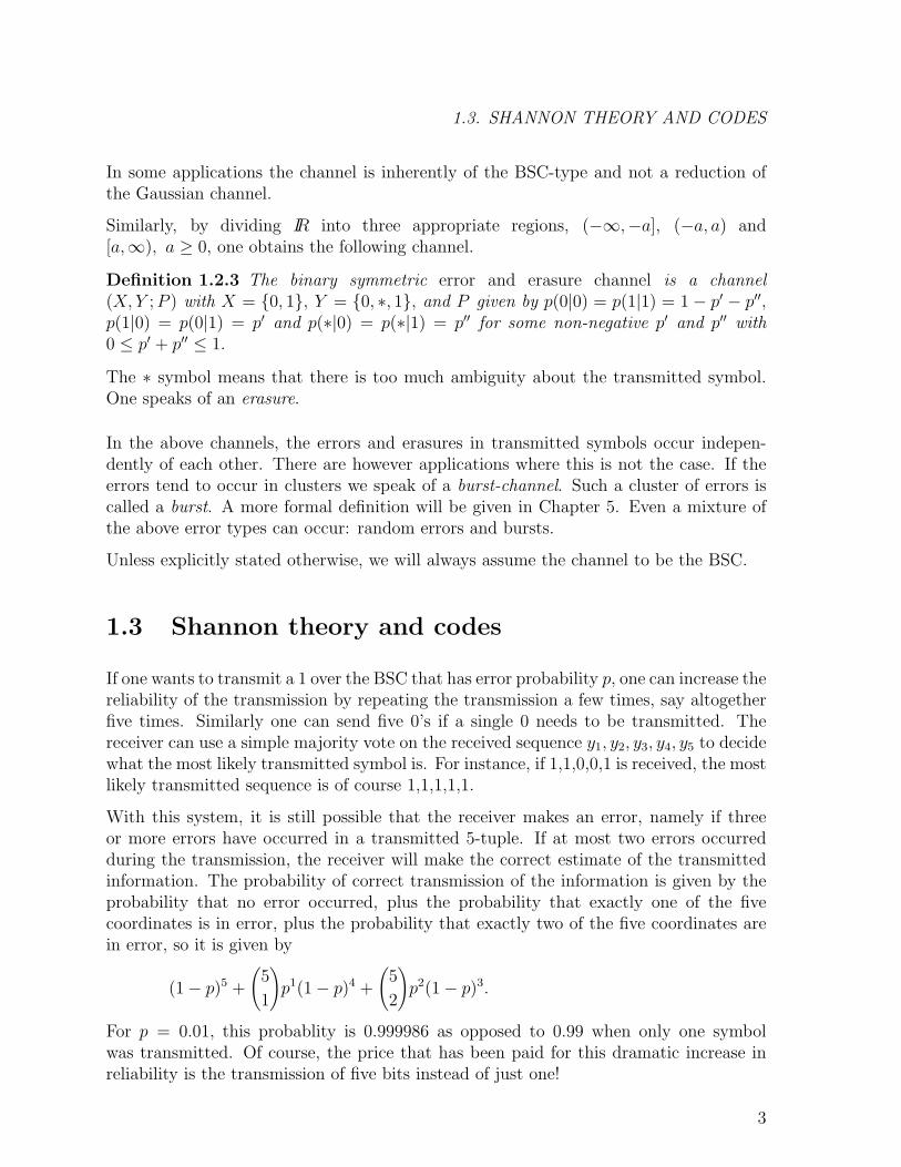
If one wants to transmit a 1 over the BSC that has error probability p, one can increase thereliability of the transmission by repeating the transmission a few times, say altogetherfive times. Similarly one can send five 0’s if a single 0 needs to be transmitted. Thereceiver can use a simple majority vote on the received sequence y1, y2, y3, y4, y5 to decidewhat the most likely transmitted symbol is. For instance, if 1,1,0,0,1 is received, the mostlikely transmitted sequence is of course 1,1,1,1,1.
With this system, it is still possible that the receiver makes an error, namely if threeor more errors have occurred in a transmitted 5-tuple. If at most two errors occurredduring the transmission, the receiver will make the correct estimate of the transmittedinformation. The probability of correct transmission of the information is given by theprobability that no error occurred, plus the probability that exactly one of the fivecoordinates is in error, plus the probability that exactly two of the five coordinates arein error, so it is given by
(1− p)5 +
(5
1
)p1(1− p)4 +
(5
2
)p2(1− p)3.
For p = 0.01, this probablity is 0.999986 as opposed to 0.99 when only one symbolwas transmitted. Of course, the price that has been paid for this dramatic increase inreliability is the transmission of five bits instead of just one!
3

CHAPTER 1. A COMMUNICATION SYSTEM
sender encoder channel decoder receiver> > > >a x y a′
Figure 1.2: A communication system
Transmitting more symbols than is strictly necessary to convey the message is calledadding redundancy to the message. Regular languages know the same phenomenon. Thefact that one immediately sees the obvious misprints in a word, like ‘lacomotivf’, meansthat the word contains more letters than are strictly necessary to convey the message.The redundant letters enable us to correct the misspelling of the received word.
Definition 1.3.1 An encoder is a mapping (or algorithm) that transforms each sequenceof symbols from the message alphabet A to a sequence of symbols from the input alphabetX of the channel, in such a way that redundancy is added (to protect it better againstchannel errors).
A complete decoder is an algorithm that transforms the received sequence of symbolsof the output alphabet Y of the channel into a message stream over A. If a decodersometimes fails to do this (because it is not able to do so or to avoid messages that aretoo unreliable) one speaks of an incomplete decoder.
The channel, encoder, and decoder, together with the sender and receiver, form a so-called communication system. See Figure 1.2, where a denotes the message stream, x asequence of letters in X, y a sequence of letters in Y and a′ a message stream.
A decoder that always finds the most likely (in terms of the channel probabilities) trans-mitted message stream a′, given the received sequence y, is called a maximum likelihooddecoder. The decoder that was described above for the encoder that repeated eachinformation bit five times is an example of a maximum likelihood decoder.
In Section 1.2 we have seen how the reduction of the Gaussian channel to the BSC throwsaway (valuable) information. A decoder that uses the output of this (reduced) BSC asits input is called a hard decision decoding algorithm, while it is called a soft decisiondecoding algorithm otherwise.
A final distinction is the one between encoders (and decoders) with and without memory.
Definition 1.3.2 If the encoder maps k-tuples of symbols from the message alphabet Ain a one-to-one way to n-tuples of symbols from the input alphabet X of the channel(independent of the other input k-tuples), the resulting set of |A|k output n-tuples iscalled a block code. For the elements of a block code one uses the name codeword.
Definition 1.3.3 If the encoder maps k-tuples of symbols from the message alphabetA to n-tuples of symbols from the input alphabet X of the channel in a way that alsodepends on the last m input k-tuples, where m is some fixed parameter, the resulting
4
1.3. SHANNON THEORY AND CODES
sequence of output n-tuples is called a convolutional code. These output sequences arealso named codewords.
For a long stream of message symbols, one of course has to break it up into segments oflength k each before they can be handled by the encoder.
Convolutional codes will be discussed in Chapter 6. Block codes form the main topicof this book. They will be extensively discussed in Chapters 2–5. Note that the codediscussed before, in which each message symbol is repeated four times, is an example ofa block code with k = 1 and n = 5.
Let M denote the size of A and let q denote the size of X. If all k-tuples of M -arysymbols are equally likely, one needs dk log2Me bits to denote one of them. This maynot be so obvious in general, but when M is some power of 2, this is a straightforwardobservation. Similarly for each of qn equally likely n-tuples of q-ary symbols one needsn log2 q bits. Let the information rate R denote the amount of information that an inputsymbol of the channel contains. It follows that
R =k log2M
n log2 q. (1.1)
If q = 2, this reduces to R = k log2 Mn
.
If q = M, equation (1.1) simplifies to R = k/n. The interpretation of the information ratein this case corresponds with the intuitive interpretation: if k information symbols aremapped into n channel input symbols from the same alphabet, the information densityin these channel input symbols is k/n.
By using block and convolutional codes, the sender wants to get information to thereceiver in a more reliable way than without using the codes. By repeating each in-formation symbol sufficiently many times, one can achieve this and obtain a reliabilityarbitrarily close to 1. However, the price that one pays is the inefficient use of thechannel: the rate of this sequence of codes tends to zero!
What Shannon was able to prove in 1948 (see: Shannon, C.E., A mathematical theory ofcommunication, Bell Syst. Tech. J., 27, pp. 379-423, 623-656, 1948) is that, as long asthe rate R is smaller than some quantity C, one can (for sufficiently long block lengthsn) find encodings at rate R, such that the probability of incorrect decoding (when usingmaximum likelihood decoding) can be made arbitrarily small, while this is not possiblefor rates above that quantity! This result forms the foundation of the whole theory oferror-correcting codes.
Definition 1.3.4 The entropy function h(p) is defined for 0 ≤ p ≤ 1 by
h(p) =
{−p log2 p− (1− p) log2(1− p), if 0 < p < 1,0, if p = 0 or 1.
(1.2)
5
CHAPTER 1. A COMMUNICATION SYSTEM
0 .5 10
1
pppppppppppppppppppppppppppppppppppppppppppppppppppppppppppppppppppppppppppppppppppppppppppppppppppppppppppppppppppppppppppppppppppppppppppppppppppppppppppppppppppppp
ppppppppppppppppppppppppppppppppppppppppppppppppppppppppppppppppppppppppppppppppppppppppppppppppppppppppppppppppppppppppppppppppppppppppppppppppppppppppppppppppppppppppppppppppppppppppppppppppppppppppppppppppppppppppppppppppppppppppppppppppppppppppppppppppppppppppppppppppppppppppppppppppppppppppppppppppppppppppppppppppppppppppppppppppppppppppppppppppppppppppppppppppppppppppppppppppppppppppppppppppppppppppppp
0 .5 10
1 pppppppppppppppppppppppppppppppppppppppppppppppppppppppppppppppppppppppppppppppppppppppppppppppppppppppppppppppppppppppppppppppppppppppppppppppppppppppppppppppppppppppppppppppppppppppppppppppppppppppppppppppppppppppppppppppppppppppppppppppppppppppppppppppppppppppppppppppppppppppppppppppppppppppppppppppppppppppppppppppppppppppppppppppppppppppppppppppppppppppppppppppppppppppppppppppppppppppppppppppppppppppppppppppppppp
ppppppppppppppppppppppppppppppppppppppppppppppppppppppppppppppppppppppppppppppppppppppppppppppppppppppppppppppppppppppppppppppppppppppppppppppppppppppppppppp
p
(a): h(p) (b): C = 1− h(p)
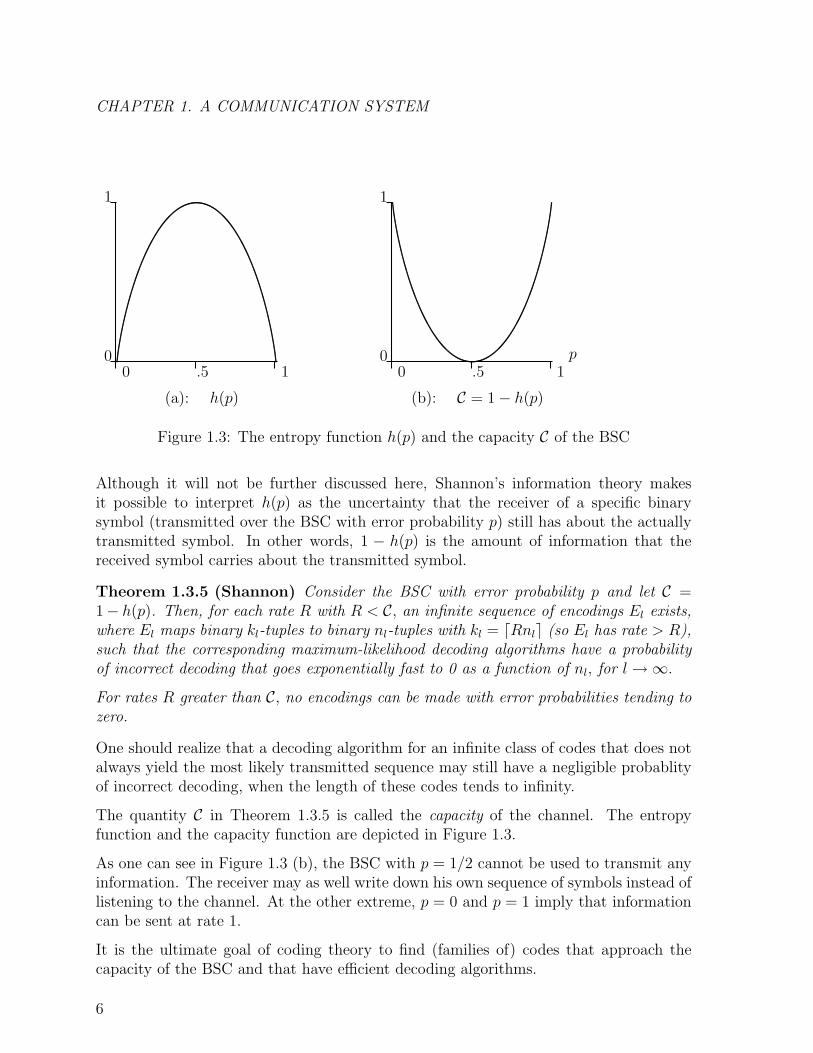
Figure 1.3: The entropy function h(p) and the capacity C of the BSC
Although it will not be further discussed here, Shannon’s information theory makesit possible to interpret h(p) as the uncertainty that the receiver of a specific binarysymbol (transmitted over the BSC with error probability p) still has about the actuallytransmitted symbol. In other words, 1 − h(p) is the amount of information that thereceived symbol carries about the transmitted symbol.
Theorem 1.3.5 (Shannon) Consider the BSC with error probability p and let C =1− h(p). Then, for each rate R with R < C, an infinite sequence of encodings El exists,where El maps binary kl-tuples to binary nl-tuples with kl = dRnle (so El has rate > R),such that the corresponding maximum-likelihood decoding algorithms have a probabilityof incorrect decoding that goes exponentially fast to 0 as a function of nl, for l→∞.
For rates R greater than C, no encodings can be made with error probabilities tending tozero.
One should realize that a decoding algorithm for an infinite class of codes that does notalways yield the most likely transmitted sequence may still have a negligible probablityof incorrect decoding, when the length of these codes tends to infinity.
The quantity C in Theorem 1.3.5 is called the capacity of the channel. The entropyfunction and the capacity function are depicted in Figure 1.3.
As one can see in Figure 1.3 (b), the BSC with p = 1/2 cannot be used to transmit anyinformation. The receiver may as well write down his own sequence of symbols instead oflistening to the channel. At the other extreme, p = 0 and p = 1 imply that informationcan be sent at rate 1.
It is the ultimate goal of coding theory to find (families of) codes that approach thecapacity of the BSC and that have efficient decoding algorithms.
6
1.4. PROBLEMS
1.4 Problems
1.4.1 Suppose that four messages are encoded into 000000, 001111, 110011 and 111100.These four messages are transmitted with equal probablity over a BSC with errorprobability p. If one receives a sequence different from the four sequences above,one knows that errors have been made during the transmission.
What is the probability that errors have been made during the transmission andthat the receiver will not find out?
1.4.2 Suppose that either (−1,−1,−1) or (+1,+1,+1) is transmitted (each with prob-ability 1/2) over the Gaussian channel defined by the density function
p(y|x) =1√2πe−(y−x)2/2.
What is the most likely transmitted sequence when the word (−1,+0.01,+0.01)is received?
What is the answer to this question if a maximum likelihood, hard decision de-coding algorithm has been applied?
7

CHAPTER 1. A COMMUNICATION SYSTEM
8
Chapter 2
Linear block codes
2.1 Block codes
In this chapter, block codes for the q-ary symmetric channel will be introduced. Let nbe fixed and let the input and output symbols of the channel belong to an alphabet Qof cardinality q. The set of Q-ary n-tuples is denoted by Qn.
A distance metric on Qn that reflects the properties of the q-ary symmetric channel verywell, is the following.
Definition 2.1.1 The Hamming distance d(x,y) between x= (x1, x2, . . . , xn) and y=(y1, y2, . . . , yn) in Qn is given by
d(x,y) = |{1 ≤ i ≤ n | xi 6= yi}|. (2.1)
In words: d(x,y) is the number of coordinates, where x and y differ. It follows fromthe properties of the q-ary symmetric channel that the more x and y differ, the moreunlikely one will be received if the other was transmitted.
It is very simple to verify that d(x,x) = 0, d(x,y) = d(y,x) and that the triangleinequality holds: d(x, z) ≤ d(x,y) + d(y, z) for any x,y and z in Qn. So the Hammingdistance is indeed a distance function.
A q-ary block code C of length n is any nonempty subset of Qn. The elements of C arecalled codewords. If |C| = 1, the code is called trivial. Quite often one simply speaks ofa “code” instead of a “block code”.
To maximize the error-protection, one needs codewords to have sufficient mutual dis-tance.
Definition 2.1.2 The minimum distance d of a non-trivial code C is given by
d = min{d(x,y) | x ∈ C,y ∈ C,x 6= y}. (2.2)
9
CHAPTER 2. LINEAR BLOCK CODES
The error-correcting capability e is defined by
e =
⌊d− 1
2
⌋. (2.3)
The reason for the name error-correcting capability is quite obvious. If d is the minimumdistance of a code C and if during the transmission of the codeword c over the channelat most e errors have been made, the received word r will still be closer to c than to anyother codeword. So a maximum likelihood decoding algorithm applied to r will result inc.
However, codes can also be used for error-detection. Let t be some integer, t ≤ e. Thenit follows from the definition of d that no word in Qn can be at distance at most t fromone codeword, while at the same time being at distance up to d− t− 1 from some othercodeword. This means that one can correct up to t errors, but also detect if more thant have occurred, as long as not more than d− t− 1 errors have occurred.
Similarly, a code C with minimum distance d can also be used for the simultaneouscorrection of errors and erasures. Let e and f be fixed such that 2e+ f < d. A receivedword r with at most f erasures cannot have distance ≤ e from two different codewordsc1 and c2 at the other n − f coordinates, because that would imply that d(c1, c2) ≤2e+ f < d. It follows that C is e-error, f -erasure-correcting.
A different interpretation of Definition 2.1.2 is that spheres of radius e around the code-words are disjoint. Let Br(x) denote the sphere of radius r around x, defined by{y ∈ Qn | d(y,x) ≤ r}. To determine the cardinality of Br(x) we first want to findthe number of words at distance i to x. To find these words, one needs to choose exactlyi of the n coordinates of x and replace each by one of the other q− 1 alphabet symbols.So there are
(ni
)(q − 1)i words at distance i from x and thus
|Br(x)| =r∑
i=0
(n
i
)(q − 1)i. (2.4)
Since all spheres with radius e around the |C| codewords are disjoint and there are onlyqn distinct words in Qn, we have proved the following theorem.
Theorem 2.1.3 (Hamming bound) Let C be an e-error-correcting code. Then
|C|e∑
i=0
(n
i
)(q − 1)i ≤ qn. (2.5)
Let d(x, C) denote the distance from x to the code C, so d(x, C) = min{d(x, c) | c ∈ C}.The next notion tells us how far a received word can possibly be removed from a code.
Definition 2.1.4 The covering radius ρ of a code C is given by
ρ = max{d(x, C) | x ∈ Qn}. (2.6)
10
2.1. BLOCK CODES
Since every word x in Qn is at distance at most ρ to some codeword, say c, it is alsoinside at least one of the spheres of radius ρ around the codewords (namely Bρ(c)). Sothese spheres together cover Qn. This proves the following theorem.
Theorem 2.1.5 Let C be a code with covering radius ρ then
|C|ρ∑
i=0
(n
i
)(q − 1)i ≥ qn. (2.7)
It follows from (2.5) and (2.7) that e ≤ ρ for every code. Equality turns out to bepossible!
Definition 2.1.6 An e-error-correcting code C with covering radius ρ is called perfectif
e = ρ.
A different way of saying that an e-error-correcting code C is perfect is “the spheres withradius e around the codewords cover Qn” or “every element in Qn is at distance at moste from a unique codeword”.
Equations (2.5) and (2.7) imply the following theorem.
Theorem 2.1.7 (Sphere packing bound) Let C be an e-error-correcting code. ThenC is perfect if and only if
|C|e∑
i=0
(n
i
)(q − 1)i = qn. (2.8)
We have already seen a code that is perfect: the binary code of length 5 with just thetwo codewords (0, 0, 0, 0, 0) and (1, 1, 1, 1, 1). It is a special example of what is called theq-ary repetition code of length n:
C = {(n︷ ︸︸ ︷
c, c, . . . , c) | c ∈ Q}.
This code has minimum distance d = n. So, for odd n the code has e = (n−1)/2. In thebinary case one can take Q = {0, 1} and gets C = {0,1}, where 0 = (0, 0, . . . , 0) and1 = (1, 1, . . . , 1). It follows that a word with at most (n− 1)/2 coordinates equal to 1, isin B(n−1)/2(0), but not in B(n−1)/2(1), while a word with at least (n + 1)/2 coordinatesequal to 1, is in B(n−1)/2(1), but not in B(n−1)/2(0). This means that ρ = (n− 1)/2 = eand that the binary repetition code of odd length is perfect.
Instead of stating that C is a code of length n, minimum distance d and cardinality M ,we shall just say that C is a (n,M, d) code.
Clearly if one applies the same coordinate permutation to all the codewords of C oneobtains a new code C ′ that has the same parameters as C. The same is true if for eachcoordinate one allows a permutation of the symbols in Q. Codes that can be obtained
11
CHAPTER 2. LINEAR BLOCK CODES
from each other in this way are called equivalent. From a coding theoretic point of viewthey are the same.
The rate of a q-ary code C of length n is defined by
R =logq |C|
n. (2.9)
This definition coincides with (1.1), if one really maps q-ary k-tuples into q-ary n-tuples(then R = k/n), but it also coincides with (1.1) in general. Indeed, if the encoder in(1.3.1) has an input alphabet of size |C| and maps each input symbol onto a uniquecodeword (so k = 1 and M = |C|), equation (1.1) reduces to (2.9).
Before we end this section, two more bounds will be given.
Theorem 2.1.8 (Singleton bound) Let C be a q-ary (n,M, d) code. Then
M ≤ qn−d+1. (2.10)
Proof: Erase in every codeword the last d − 1 coordinates. Because all codewordsoriginally have distance at least d, the new words will still all be distinct. Their lengthis n − d + 1. However, there are only qn−d+1 distinct words of length n − d + 1 over analphabet of size q.
2
Codes with parameters (n, qn−d+1, d) (i.e. for which the Singleton bound holds withequality) are called maximum-distance-separable codes or simply MDS codes.
Now that we have seen several bounds that give an upper bound on the size of a codein terms of n and d, it is good to know that also lower bounds exist.
Theorem 2.1.9 (Gilbert-Varshamov bound) There exist q-ary (n,M, d) codes sat-isfying
M ≥ qn∑d−1i=0
(ni
)(q − 1)i
. (2.11)
Proof: As long as a q-ary (n,M, d) code C satisfies M < qn∑d−1
i=0 (ni)(q−1)i
the spheres with
radius d − 1 around the words in C will not cover the set of all q-ary n-tuples, so onecan add a word to C that has distance at least d to all elements of C.
2
2.2 Linear codes
If one assumes the alphabet Q and the code C to have some internal structure, one canconstruct and analyze codes much more easily than in the absence of such structures.
12
2.2. LINEAR CODES
From now on Q will always have the structure of the Galois field GF (q), the finite fieldwith q elements (for the reader who is not familiar with finite fields Appendix A isincluded). As a consequence q = pm for some prime p. Very often q will simply be 2.
Now that Q = GF (q), we can associate the set of words Qn with an n-dimensional vectorspace over GF (q). It will be denoted by Vn(q). For Vn(2) we shall simply write Vn. Theelements in Vn(q) are of course vectors, but will occasionally still be called words. Thesymbols denoting vectors will be underlined.
If a codeword c has been transmitted but the vector r is received, the error pattern,caused by the channel, is the vector e with
r = c+ e. (2.12)
The addition in (2.12) denotes the vector addition in Vn(q). The number of errors thatoccurred during the transmission is the number of non-zero entries in e.
Definition 2.2.1 The Hamming weight w(x) of a vector x is the number of non-zerocoordinates in x. So
w(x) = d(x, 0).
Now that Qn has the structure of the vector space Vn(q), we can define the most impor-tant general class of codes.
Definition 2.2.2 A linear code C of length n is any linear subspace of Vn(q).
If C has dimension k and minimum distance d, one says that C is an [n, k, d] code.
Note that a q-ary (n,M, d) code C has cardinality M, while a q-ary [n, k, d] code C islinear and has cardinality qk. The parameter d in the notations (n,M, d) and [n, k, d] issometimes omitted.
To determine the minimum distance of an unstructured (n,M, d) code C one has to
compute the distance between all(
M2
)pairs of codewords. For linear codes without
further structure, the next theorem will prove that this complexity is only M − 1. Thisis the first bonus of the special structure of linear codes.
Theorem 2.2.3 The minimum distance of a linear code C is equal to the minimumnon-zero weight in C.
Proof: Since C is linear, with x and y in C also x− y is in C. The theorem now followsfrom the two observations:
d(x, y) = d(x− y, 0) = w(x− y),
w(x) = d(x, 0),
which state that the distance between any two distinct codewords is equal to the weightof some non-zero codeword and vice versa.
13
CHAPTER 2. LINEAR BLOCK CODES
2
So, to determine the minimum distance of a linear code, one never needs to do morethan to find the lowest weight of all M − 1 non-zero codewords.
There are two standard ways of describing a k-dimensional linear subspace: one by meansof k independent basis vectors, the other uses n−k linearly independent equations. Bothtechniques turn out to be quite powerful in this context.
Definition 2.2.4 A generator matrix G of an [n, k, d] code C is a k×n matrix, of whichthe k rows form a basis of C. One says “the rows of G generate C”.
It follows that
C = {aG | a ∈ Vk(q)} (2.13)
The codeword c = aG in (2.13) is the result of the encoding algorithm “multiplicationby G” applied to the so-called information vector or message vector a.
Example 2.2.5 A generator matrix of the q-ary [n, 1, n] repetition code is given by
G = (1 1 · · · · · · 1).
Example 2.2.6 The binary even weight code is defined as the set of all words of evenweight. It is a linear code with parameters [n, n− 1, 2]. A generator matrix of the evenweight code is given by
G =
1 0 0 · · · · · · 0 10 1 0 · · · · · · 0 10 0 1 · · · · · · 0 1...
......
. . ....
......
......
. . ....
...0 0 0 · · · · · · 1 1
.
Examples 2.2.5 and 2.2.6 are also examples of what is called a generator matrix instandard form, i.e. a generator matrix of the form (Ik P ), where Ik is the k× k identitymatrix. If G is in standard form, the first k coordinates of a codeword aG producethe information vector a itself! For this reason these coordinates are called informationsymbols. The last n − k coordinates are added to the k information symbols to makeerror-correction possible.
Since the generator matrix of a linear code has full row rank, it is quite obvious that anylinear code is equivalent to a linear code that does have a generator matrix in standardform. The quantity r = n− k is called the redundancy of the code.
Non-linear codes of cardinality qk sometimes also have the property that on the firstk coordinates all qk possible (information) sequences occur. These codes are calledsystematic on the first k coordinates. It follows from the proof of the Singleton bound
14
2.2. LINEAR CODES
(Theorem 2.1.8) that MDS codes are systematic on every k-tuple of coordinates. Alsothe converse holds (see Problem 2.5.10).
The second way of describing linear codes is as follows.
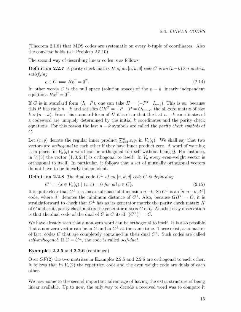
Definition 2.2.7 A parity check matrix H of an [n, k, d] code C is an (n−k)×n matrix,satisfying
c ∈ C ⇐⇒ HcT = 0T . (2.14)
In other words C is the null space (solution space) of the n − k linearly independentequations HxT = 0T .
If G is in standard form (Ik P ), one can take H = (−P T In−k). This is so, becausethis H has rank n− k and satisfies GHT = −P +P = Ok,n−k, the all-zero matrix of sizek × (n− k). From this standard form of H it is clear that the last n− k coordinates ofa codeword are uniquely determined by the initial k coordinates and the parity checkequations. For this reason the last n− k symbols are called the parity check symbols ofC.
Let (x, y) denote the regular inner product∑n
i=1 xiyi in Vn(q). We shall say that twovectors are orthogonal to each other if they have inner product zero. A word of warningis in place: in Vn(q) a word can be orthogonal to itself without being 0. For instance,in V4(3) the vector (1, 0, 2, 1) is orthogonal to itself! In Vn every even-weight vector isorthogonal to itself. In particular, it follows that a set of mutually orthogonal vectorsdo not have to be linearly independent.
Definition 2.2.8 The dual code C⊥ of an [n, k, d] code C is defined by
C⊥ = {x ∈ Vn(q) | (x, c) = 0 for all c ∈ C}. (2.15)
It is quite clear that C⊥ is a linear subspace of dimension n−k. So C⊥ is an [n, n−k, d⊥]code, where d⊥ denotes the minimum distance of C⊥. Also, because GHT = O, it isstraightforward to check that C⊥ has as its generator matrix the parity check matrix Hof C and as its parity check matrix the generator matrixG of C. Another easy observationis that the dual code of the dual of C is C itself: (C⊥)⊥ = C.
We have already seen that a non-zero word can be orthogonal to itself. It is also possiblethat a non-zero vector can be in C and in C⊥ at the same time. There exist, as a matterof fact, codes C that are completely contained in their dual C⊥. Such codes are calledself-orthogonal. If C = C⊥, the code is called self-dual.
Examples 2.2.5 and 2.2.6 (continued)
Over GF (2) the two matrices in Examples 2.2.5 and 2.2.6 are orthogonal to each other.It follows that in Vn(2) the repetition code and the even weight code are duals of eachother.
We now come to the second important advantage of having the extra structure of beinglinear available. Up to now, the only way to decode a received word was to compare it
15
CHAPTER 2. LINEAR BLOCK CODES
with all codewords and find the closest. This technique has complexity |C| and thus forq-ary [n, k, d] codes complexity qk.
Definition 2.2.9 Let C be a q-ary [n, k, d] code with parity check matrix H. The syn-drome s of a vector x in Vn(q) is the vector in Vn−k(q) defined by s = HxT .
Note that a syndrome s is a column vector, while the vectors related to transmitted orreceived words are row vectors.
If the syndrome of a received word r is 0, then r is a codeword and most likely no errorhas occurred during the transmission.
In general, if the codeword c has been transmitted and the word r = c + e has beenreceived, where e is the error pattern, one has
HrT = H(c+ e)T = HcT +HeT = HeT . (2.16)
So, the syndrome of r is completely determined by that of e. The real decoding problemis how to find the codeword c that is closest to the received word r, in other words tofind a vector e of minimal weight, such that r − e is in C.
Now let s in Vn−k(q) be the syndrome of a received word r. Then not just r is a solutionof s = HxT , but all vectors r + c with c in C form the solution space of this system oflinear equations. The set {r+ c | c in C} forms a coset of C in the additive group Vn(q).We need to find a vector e of minimal weight in this coset. This minimum weight wordin the coset is called the coset leader of the coset. As we shall see later, this coset leaderdoes not have to be unique. However, if C is e-error-correcting, each word of weight atmost e will be the unique coset leader of a unique coset. Indeed if two distinct wordsof weight at most e would lie in the same coset, their difference would be a codeword ofweight at most 2e, a contradiction with the minimum distance of C, which is 2e + 1 or2e+ 2.
Once e has been found, the codeword c = r−e is a good maximum-likelihood estimate ofthe transmitted codeword, in the sense that no other codeword has a higher probabilityof being transmitted. That r − e is indeed a codeword, follows from the fact thatboth vectors have the same syndrome, so their difference has syndrome 0, i.e. is in C. Itfollows from the above that the next algorithm is indeed a maximum-likelihood decodingalgorithm for each linear code.
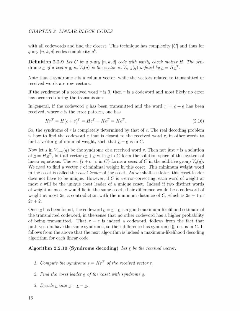
Algorithm 2.2.10 (Syndrome decoding) Let r be the received vector.
1. Compute the syndrome s = HrT of the received vector r.
2. Find the coset leader e of the coset with syndrome s.
3. Decode r into c = r − e.
16
2.2. LINEAR CODES
Once one has made a table of all syndromes with a corresponding coset leader, Algorithm2.2.10 yields a maximum-likelihood decoding algorithm with complexity qn−k. So fork > n/2, this algorithm is faster than the brute-force approach of comparing the receivedword with all qk codewords. In subsequent chapters we shall meet codes with decodingalgorithms that do not have an exponentially-fast growing complexity.
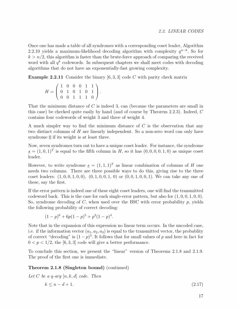
Example 2.2.11 Consider the binary [6, 3, 3] code C with parity check matrix
H =
1 0 0 0 1 10 1 0 1 0 10 0 1 1 1 0
.That the minimum distance of C is indeed 3, can (because the parameters are small inthis case) be checked quite easily by hand (and of course by Theorem 2.2.3). Indeed, Ccontains four codewords of weight 3 and three of weight 4.
A much simpler way to find the minimum distance of C is the observation that anytwo distinct columns of H are linearly independent. So a non-zero word can only havesyndrome 0 if its weight is at least three.
Now, seven syndromes turn out to have a unique coset leader. For instance, the syndromes = (1, 0, 1)T is equal to the fifth column in H, so it has (0, 0, 0, 0, 1, 0) as unique cosetleader.
However, to write syndrome s = (1, 1, 1)T as linear combination of columns of H oneneeds two columns. There are three possible ways to do this, giving rise to the threecoset leaders: (1, 0, 0, 1, 0, 0), (0, 1, 0, 0, 1, 0) or (0, 0, 1, 0, 0, 1). We can take any one ofthese, say the first.
If the error pattern is indeed one of these eight coset leaders, one will find the transmittedcodeword back. This is the case for each single-error pattern, but also for (1, 0, 0, 1, 0, 0).So, syndrome decoding of C, when used over the BSC with error probability p, yieldsthe following probability of correct decoding:
(1− p)6 + 6p(1− p)5 + p2(1− p)4.
Note that in the expansion of this expression no linear term occurs. In the uncoded case,i.e. if the information vector (a1, a2, a3) is equal to the transmitted vector, the probablityof correct “decoding” is (1− p)3. It follows that for small values of p and here in fact for0 < p < 1/2, the [6, 3, 3] code will give a better performance.
To conclude this section, we present the “linear” version of Theorems 2.1.8 and 2.1.9.The proof of the first one is immediate.
Theorem 2.1.8 (Singleton bound) (continued)
Let C be a q-ary [n, k, d] code. Then
k ≤ n− d+ 1. (2.17)
17
CHAPTER 2. LINEAR BLOCK CODES
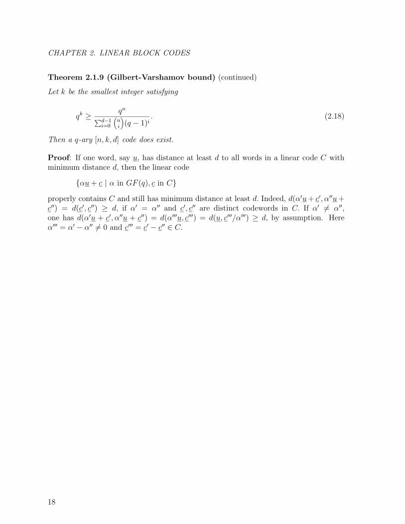
Theorem 2.1.9 (Gilbert-Varshamov bound) (continued)
Let k be the smallest integer satisfying
qk ≥ qn∑d−1i=0
(ni
)(q − 1)i
. (2.18)
Then a q-ary [n, k, d] code does exist.
Proof: If one word, say u, has distance at least d to all words in a linear code C withminimum distance d, then the linear code
{αu+ c | α in GF (q), c in C}
properly contains C and still has minimum distance at least d. Indeed, d(α′u+ c′, α′′u+c′′) = d(c′, c′′) ≥ d, if α′ = α′′ and c′, c′′ are distinct codewords in C. If α′ 6= α′′,one has d(α′u + c′, α′′u + c′′) = d(α′′′u, c′′′) = d(u, c′′′/α′′′) ≥ d, by assumption. Hereα′′′ = α′ − α′′ 6= 0 and c′′′ = c′ − c′′ ∈ C.
18
2.3. THE MACWILLIAMS RELATIONS
Starting with C = {0} apply the above argument repeatedly until (2.18) is met.
2
2.3 The MacWilliams relations
When studying properties of a linear code, it is often important to know how manycodewords have a certain weight (in particular this is true for the weights close to d).
Definition 2.3.1 Let C be a code. Then the weight enumerator A(z) of C is given by
A(z) =n∑
i=0
Aizi =
∑c∈C
zw(c). (2.19)
So, Ai, 0 ≤ i ≤ n, counts the number of code words of weight i in C.
For instance, the q-ary repetition code of length n has weight enumerator 1 + (q− 1)zn.The code in Example 2.2.11 has weight enumerator 1 + 4z3 + 3z4.
In 1963, F.J. MacWilliams showed that the weight enumerators of a linear code C andof its dual code C⊥ are related by a rather simple formula. This relation will turn outto be a very powerful tool.
We need a definition and a lemma first.
Definition 2.3.2 A character χ of GF (q) is a mapping of GF (q) to the set of complexnumbers with absolute value 1, satisfying
χ(α+ β) = χ(α)χ(β) for all α and β in GF (q). (2.20)
The principal character maps every field element to 1.
It follows from χ(0) = χ(0 + 0) = χ2(0) that χ(0) = 1.
An example of a non-principal character χ of GF (p) = {0, 1, . . . , p − 1} is given byχ(a) = expa2πi/p . It is also quite easy to find a non-principal character of GF (q). Forinstance, ifGF (q) has characteristic p and ω is a complex, primitive p-th root of unity, thefunction χ(α) = ωA(α), where A is any non-trivial linear mapping from GF (q) to GF (p),will define a non-principal character of GF (q). When representing GF (q), q = pm, as anm-dimensional vector space over GF (p) the projection on the first coordinate alreadygives such a mapping. Also the trace-function Tr, defined by Tr(x) = x+ xp + . . . xpm−1
is such a mapping (see also Problem A.6.19). The fact however is that below we do needto make an explicit choice for χ.
Lemma 2.3.3 Let χ be a character of GF (q). Then∑α∈GF (q)
χ(α) =
{q, if χ is the principal character,0, otherwise.
(2.21)
19
CHAPTER 2. LINEAR BLOCK CODES
Proof: For the principal character the assertion is trivial. For a non-principal character,take β in GF (q) such that χ(β) 6= 1. Then
χ(β)∑
α∈GF (q)
χ(α) =∑
α∈GF (q)
χ(α+ β) =∑
α∈GF (q)
χ(α).
This equation can be rewritten as (1 − χ(β))∑
α∈GF (q) χ(α) = 0. Since χ(β) 6= 1 theassertion follows.
2
Theorem 2.3.4 (MacWilliams) Let A(z) be the weight enumerator of a q-ary, linearcode C and let B(z) be the weight enumerator of the dual code C⊥. Then
B(z) =1
|C|(1 + (q − 1)z)nA
(1− z
1 + (q − 1)z
)=
=1
|C|
n∑i=0
Ai(1− z)i(1 + (q − 1)z)n−i. (2.22)
Proof: Let χ be a non-principal character of GF (q). We shall evaluate the expression∑c∈C
∑u∈Vn(q)
χ((c, u))zw(u). (2.23)
in two different ways, obtaining in this way the left hand and the right hand sides in(2.22).
Changing the order of summation in (2.23) yields∑u∈Vn(q)
zw(u)∑c∈C
χ((c, u)). (2.24)
The inner sum in (2.24) is equal to |C|, when u is an element in C⊥, because all innerproducts (c, u) are zero in this case. However, if u is not an element in C⊥, the innerproducts (c, u) take on each value in GF (q) equally often (by the linearity of the innerproduct). It follows from Lemma 2.3.3 that the inner sum in (2.24) is now equal to 0.So (2.24), and thus also (2.23), is equal to∑
u∈C⊥
zw(u)|C| = |C|B(z), (2.25)
by Definition 2.3.1 applied to C⊥.
Now we shall evaluate (2.23) in a different way.The inner sum of (2.23)
∑u∈Vn(q) χ((c, u))zw(u) is equal to
∑(u1,u2,...,un)∈Vn(q)
χ(c1u1 + c2u2 + · · ·+ cnun)zw((u1,u2,···,un)) =
∑u1∈V1(q)
· · ·∑
un∈V1(q)
χ(c1u1) · · ·χ(cnun)zw(u1) · · · zw(un) =
20
2.3. THE MACWILLIAMS RELATIONS
n∏i=1
∑ui∈V1(q)
χ(ciui)zw(ui). (2.26)
The inner sum in this last expression is equal to 1 + (q− 1)z if ci = 0. If ci 6= 0 the innersum is equal to
1 + z∑α 6=0
χ(α) = 1− zχ(0) = 1− z,
by Lemma 2.3.3.
So, the inner sum in (2.23) is equal to (1 − z)w(c)(1 + (q − 1)z)n−w(c) and thus (byDefinition 2.3.1) Equation (2.23) can be rewritten as
n∑i=0
Ai(1− z)i(1 + (q − 1)z)n−i.
Setting this equal to (2.25) proves the theorem.
2
Instead of finding the weight enumerator of a [n, k, d] code with k > n/2 directly, it is of-ten easier to find the weight enumerator of its dual code and then apply the MacWilliamsrelation.
Examples 2.2.5 and 2.2.6 (continued)
The weight enumerator of the repetition code is 1 + (q − 1)zn. So its dual has weightenumerator
1
q{(1 + (q − 1)z)n + (q − 1)(1− z)n} .
In particular in the binary case, it follows that the even weight code has weight enumer-ator
1
2{(1 + z)n + (1− z)n} =
∑i even
(n
i
)zi.
Of course, the fact that the even weight code does not contain odd weight words anddoes contain all even weight words just is the definition of this code.
A more interesting example of the MacWilliams relations will be given in the next chap-ter.
The weight enumerator A(z) of a binary linear code C is very helpful when studyingthe probability Pre that a maximum likelihood decoder makes a decoding error, i.e. theprobability that, while one codeword has been transmitted, the received word is in factcloser to another codeword.
21
CHAPTER 2. LINEAR BLOCK CODES
By the linearity of C we may assume that 0 was the transmitted codeword. Let c bea non-zero codeword of weight w. Let Pre(c) denote the probability that the receivedvector is closer to c than to 0, though 0 was transmitted. Then
Pre(c) =∑
i≥dw/2e
(w
i
)pi(1− p)w−i.
Now the probablity Pre of incorrectly decoding can be bounded above as follows
Pre ≤∑
c∈C,c 6=0Pre(c).
It follows from
∑i≥dw/2e
(w
i
)pi(1− p)w−i ≤ pw/2(1− p)w/2
∑i≥dw/2e
(w
i
)≤
≤ pw/2(1− p)w/22w =
= (2√p(1− p))w
that
Pre ≤∑w>0
Aw
(2√p(1− p)
)w
,
where Aw denotes the number of codewords of weight w in C.
This proves the following theorem.
Theorem 2.3.5 The probablity Pre that a maximum likelihood decoding algorithm de-codes a received word incorrectly, when a codeword from a linear code with weight enu-merator A(z) has been transmitted, satisfies
Pre ≤ A(2√p(1− p)
)− 1. (2.27)
2.4 Linear unequal error protection codes
There are applications where one wants to protect some data bits better than others. Forinstance, an error in the sign or in the most significant bit in the binary representationof a number is much more serious than in the least significant bit.
It will turn out that the extra protection that one can give to some of the informationbits, when using a linear code C, depends very much on the particular generator matrixG that has been chosen.
22
2.4. LINEAR UNEQUAL ERROR PROTECTION CODES
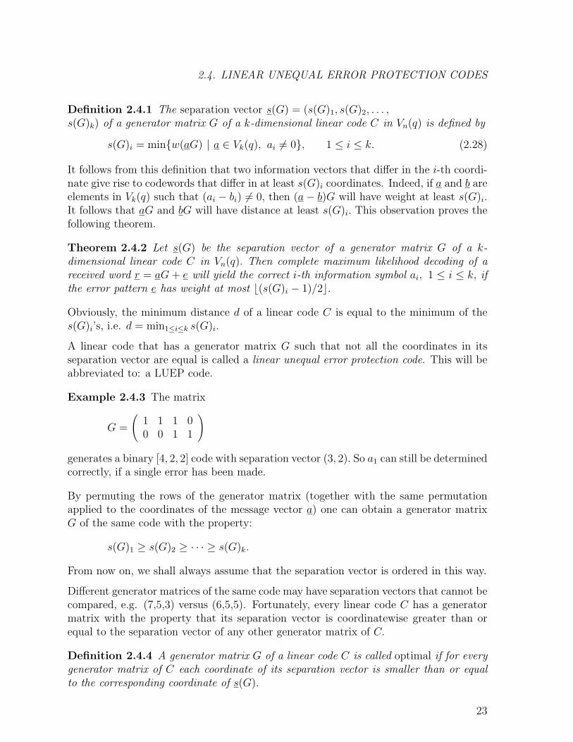
Definition 2.4.1 The separation vector s(G) = (s(G)1, s(G)2, . . . ,s(G)k) of a generator matrix G of a k-dimensional linear code C in Vn(q) is defined by
s(G)i = min{w(aG) | a ∈ Vk(q), ai 6= 0}, 1 ≤ i ≤ k. (2.28)
It follows from this definition that two information vectors that differ in the i-th coordi-nate give rise to codewords that differ in at least s(G)i coordinates. Indeed, if a and b areelements in Vk(q) such that (ai − bi) 6= 0, then (a− b)G will have weight at least s(G)i.It follows that aG and bG will have distance at least s(G)i. This observation proves thefollowing theorem.
Theorem 2.4.2 Let s(G) be the separation vector of a generator matrix G of a k-dimensional linear code C in Vn(q). Then complete maximum likelihood decoding of areceived word r = aG+ e will yield the correct i-th information symbol ai, 1 ≤ i ≤ k, ifthe error pattern e has weight at most b(s(G)i − 1)/2c.
Obviously, the minimum distance d of a linear code C is equal to the minimum of thes(G)i’s, i.e. d = min1≤i≤k s(G)i.
A linear code that has a generator matrix G such that not all the coordinates in itsseparation vector are equal is called a linear unequal error protection code. This will beabbreviated to: a LUEP code.
Example 2.4.3 The matrix
G =
(1 1 1 00 0 1 1
)
generates a binary [4, 2, 2] code with separation vector (3, 2). So a1 can still be determinedcorrectly, if a single error has been made.
By permuting the rows of the generator matrix (together with the same permutationapplied to the coordinates of the message vector a) one can obtain a generator matrixG of the same code with the property:
s(G)1 ≥ s(G)2 ≥ · · · ≥ s(G)k.
From now on, we shall always assume that the separation vector is ordered in this way.
Different generator matrices of the same code may have separation vectors that cannot becompared, e.g. (7,5,3) versus (6,5,5). Fortunately, every linear code C has a generatormatrix with the property that its separation vector is coordinatewise greater than orequal to the separation vector of any other generator matrix of C.
Definition 2.4.4 A generator matrix G of a linear code C is called optimal if for everygenerator matrix of C each coordinate of its separation vector is smaller than or equalto the corresponding coordinate of s(G).
23

CHAPTER 2. LINEAR BLOCK CODES
Clearly, if a code C has several optimal generator matrices, they will all have the sameseparation vector, called the separation vector of the code.
Of course different codes of the same length and dimension can exist that have incom-parable separation vectors. For instance the matrices
G1 =
(1 1 1 1 1 1 00 0 0 0 0 1 1
)and
G2 =
(1 1 1 1 1 0 00 0 0 1 1 1 1
)
generate 2-dimensional codes in V7 with optimal separation vectors (6, 2) resp. (5, 4).
To prove that each linear code has an optimal generator matrix, we need some notation.
Let C be a k-dimensional code in Vn(q) and letG be a generator matrix of C. The i-th rowof G will be denoted by g
i, 1 ≤ i ≤ k, and the set of rows of G by R(G). Further C[w] is
defined as the set of codewords in C of weight at most w, so C[w] = {c ∈ C | w(c) ≤ w}.Let < C[w] > be the linear span of the vectors in C[w]. Clearly,<C[w]> is a linear subcode of C. Let R(G)[w] be the smallest subset of R(G) with alinear span containing <C[w]>, i.e.
R(G)[w] = ∩ {X ⊂ R(G) | < C[w] > ⊂ <X>}.
Lemma 2.4.5 The generator matrix G of a k-dimensional code in Vn(q) satisfies
s(G)i ≤ w ⇔ gi∈ R(G)[w], (2.29)
for all 0 ≤ w ≤ n and 1 ≤ i ≤ k.
Proof:⇒: If g
i6∈ R(G)[w] then C[w] ⊂ <R(G) \ {g
i}> and hence s(G)i > w.
⇐: If gi∈ R(G)[w] then C[w] 6⊂ <R(G) \ {g
i}> . So,
C[w] ∩ (C\ <R(G) \ {gi}>) 6= ∅.
In other words, a codeword c of weight at most w exists such that αi 6= 0 in c =∑k
i=1 αigi.
So s(G)i ≤ w.
2
Lemma 2.4.6 The generator matrix G of a k-dimensional code in Vn(q) is optimal ifand only if <C[w]> = <R(G)[w]> for each 0 ≤ w ≤ n.
Proof:⇒: By the definition of <R(G)[w]> one trivially has <C[w]> ⊂ <R(G)[w]>. Let<C[w]> have rank l and let G′ be any generator matrix of C, whose last l rows generate<C[w]> . It follows that s(G′)i > w, 1 ≤ i ≤ k − l. By the optimality of G we mayconclude that s(G)i > w, 1 ≤ i ≤ k− l, and thus that <C[w]> ⊃ <g
k−l+1, · · · , g
k> .
24
2.5. PROBLEMS
It follows that <C[w]>=<R(G)[w]> .⇐: Consider any other generator matrix G′ of C and let i be minimal such that s(G′)i >s(G)i (if no such i exists, there is nothing to prove). Put w = s(G′)i− 1. From s(G′)1 ≥. . . ≥ s(G′)i > w, it follows that C[w] ⊂ <g′
i+1, . . . , g′
k> and thus that <C[w]> ⊂ <
g′i+1, . . . , g′
k> .
On the other hand, from s(G)k ≤ . . . ≤ s(G)i ≤ s(G′)i−1 = w and Lemma 2.4.5 it followsthat g
i, . . . , g
k∈ R(G)[w]. Combining these results we get the following contradiction:
gi, . . . , g
k⊂ <R(G)[w]> =
<C[w]>⊂<g′i+1, . . . , g′
k> .
2
The proof of Lemma 2.4.6 also tells us how to find an optimal generator matrix of alinear code. Consider with the set of lowest weight codewords. Take any basis of thelinear span of these vectors and fill the bottom part of the generator matrix with thesebasis vectors. Now take the set of lowest weight codewords, that are not in the span ofthe rows of G yet, and look at the linear span of them and the current rows of G. Extendthe previous basis to a basis of this new linear span. And so on.
This algorithm proves the the following theorem.
Theorem 2.4.7 Any linear code has an optimal generator matrix.
If the lowest weight codewords in a linear code generate the whole code, one obviouslydoes not have a LUEP code.
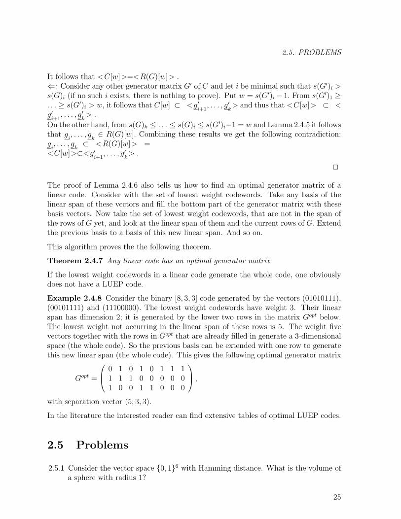
Example 2.4.8 Consider the binary [8, 3, 3] code generated by the vectors (01010111),(00101111) and (11100000). The lowest weight codewords have weight 3. Their linearspan has dimension 2; it is generated by the lower two rows in the matrix Gopt below.The lowest weight not occurring in the linear span of these rows is 5. The weight fivevectors together with the rows in Gopt that are already filled in generate a 3-dimensionalspace (the whole code). So the previous basis can be extended with one row to generatethis new linear span (the whole code). This gives the following optimal generator matrix
Gopt =
0 1 0 1 0 1 1 11 1 1 0 0 0 0 01 0 0 1 1 0 0 0
,with separation vector (5, 3, 3).
In the literature the interested reader can find extensive tables of optimal LUEP codes.
2.5 Problems
2.5.1 Consider the vector space {0, 1}6 with Hamming distance. What is the volume ofa sphere with radius 1?
25
CHAPTER 2. LINEAR BLOCK CODES
Is it possible to find 9 codewords at mutual distance at least 3?
2.5.2 Consider the BSC with error probability p. Four messages are encoded with wordsin {0, 1}6. Maximize the minimum distance of such a code. Show that such a codeis unique and equivalent to a linear code. Give the weights of all the coset leadersof this linear code. What is the probability that a transmitted codeword from thiscode will be correctly decoded by a maximum likelihood decoding algorithm.
2.5.3 Construct a (4, 9, 3) code over the alphabet {0, 1, 2}.
2.5.4 Consider a binary channel, that has a probability of p = 0.9 that a transmittedsymbol is received correctly and a probability of q = 0.1 of producing an erasure (soa ∗ is received). Construct a length-5 code of maximum cardinality that decodesany received codeword with at most one erasure correctly.
What is the probability that a codeword transmitted over this channel is decodedcorrectly?
2.5.5 Suppose that all the rows in the generator matrix G of a binary linear code Chave even weight. Prove that all codewords in C have even weight.
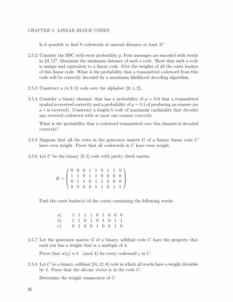
2.5.6 Let C be the binary [9, 5] code with parity check matrix
H =
0 0 0 1 1 0 1 1 01 1 0 1 1 0 0 0 00 1 1 0 1 1 0 0 00 0 0 0 1 1 0 1 1
.
Find the coset leader(s) of the cosets containing the following words:
a) 1 1 1 1 0 1 0 0 0b) 1 1 0 1 0 1 0 1 1c) 0 1 0 0 1 0 0 1 0
2.5.7 Let the generator matrix G of a binary, selfdual code C have the property thateach row has a weight that is a multiple of 4.
Prove that w(c) ≡ 0 (mod 4) for every codeword c in C.
2.5.8 Let C be a binary, selfdual [24, 12, 8] code in which all words have a weight divisibleby 4. Prove that the all-one vector is in the code C.
Determine the weight enumerator of C.
26
2.5. PROBLEMS
2.5.9 Let H be the parity check matrix of a q-ary [n, k, d] code C with covering radiusρ.
Prove that d is determined by the two properties: 1) each (d−1)-tuple of columnsof H is linearly independent and 2) H contains at least one d-tuple of linearlydependent columns.
Prove that ρ is determined by the two properties: 1) each vector in Vn−k(q) canbe written as a linear combination of some ρ-tuple of columns of H and 2) thereexists at least one vector in Vn−k(q) that cannot be written as linear combinationof any ρ− 1 columns of H.
2.5.10 Let C be an (n, qk, d = n− k+ 1) code over GF (q), i.e. C is a MDS code. Provethat C is systematic on every k-tuple of coordinates.
How many codewords of weight d does C have (as a function of n, k and q), if theall-zero word is in C.
2.5.11 Show what kind of results the Gilbert, Singleton, and Hamming Bound give whenapplied to q = 2, n = 16 and d = 3, 5, 7, 9.
Put all the results in the following table to compare them.
n = 16 d = 3 d = 5 d = 7 d = 9GilbertGilbert forlinear codesSingletonHamming
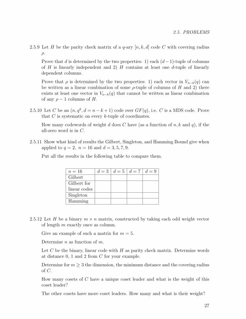
2.5.12 Let H be a binary m× n matrix, constructed by taking each odd weight vectorof length m exactly once as column.
Give an example of such a matrix for m = 5.
Determine n as function of m.
Let C be the binary, linear code with H as parity check matrix. Determine wordsat distance 0, 1 and 2 from C for your example.
Determine form ≥ 3 the dimension, the minimum distance and the covering radiusof C.
How many cosets of C have a unique coset leader and what is the weight of thiscoset leader?
The other cosets have more coset leaders. How many and what is their weight?
27
CHAPTER 2. LINEAR BLOCK CODES
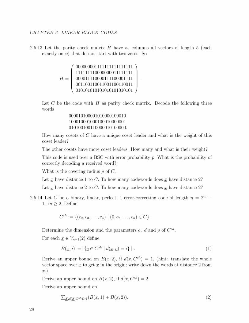
2.5.13 Let the parity check matrix H have as columns all vectors of length 5 (eachexactly once) that do not start with two zeros. So
H =
000000001111111111111111111111110000000011111111000011110000111100001111001100110011001100110011010101010101010101010101
.
Let C be the code with H as parity check matrix. Decode the following threewords
000010100001010000100010100010001000100010000001010100100110000010100000.
How many cosets of C have a unique coset leader and what is the weight of thiscoset leader?
The other cosets have more coset leaders. How many and what is their weight?
This code is used over a BSC with error probability p. What is the probability ofcorrectly decoding a received word?
What is the covering radius ρ of C.
Let x have distance 1 to C. To how many codewords does x have distance 2?
Let x have distance 2 to C. To how many codewords does x have distance 2?
2.5.14 Let C be a binary, linear, perfect, 1 error-correcting code of length n = 2m −1, m ≥ 2. Define
Csh := {(c2, c3, . . . , cn) | (0, c2, . . . , cn) ∈ C}.
Determine the dimension and the parameters e, d and ρ of Csh.
For each x ∈ Vn−1(2) define
B(x, i) :=| {c ∈ Csh | d(x, c) = i} | . (1)
Derive an upper bound on B(x, 2), if d(x,Csh) = 1. (hint: translate the wholevector space over x to get x in the origin; write down the words at distance 2 fromx.)
Derive an upper bound on B(x, 2), if d(x,Csh) = 2.
Derive an upper bound on∑x,d(x,Csh)≥1(B(x, 1) +B(x, 2)). (2)
28
2.5. PROBLEMS
Compute this sum exactly by substituting (1) into (2), followed by changing theorder of summation.
Compare the two answers. What is your conclusion for the upper bounds onB(x, 2)?
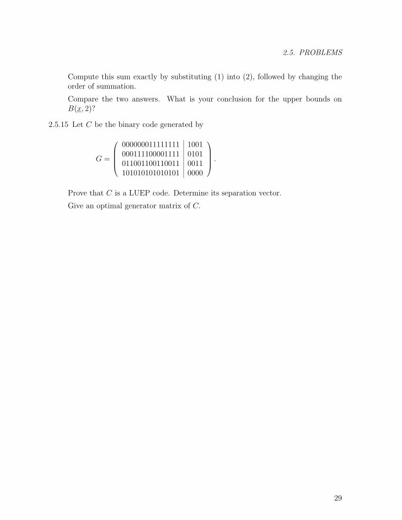
2.5.15 Let C be the binary code generated by
G =
000000011111111 1001000111100001111 0101011001100110011 0011101010101010101 0000
.
Prove that C is a LUEP code. Determine its separation vector.
Give an optimal generator matrix of C.
29

CHAPTER 2. LINEAR BLOCK CODES
30
Chapter 3
Some code constructions
3.1 Making codes from other codes
In this section, a number of techniques to construct other codes from a given code willbe discussed.
Definition 3.1.1 Let C be a q-ary (n,M, d) code. The extended code Cext of C isdefined by
Cext = {(c1, c2, . . . , cn,−n∑
i=1
ci) | c in C} (3.1)
So, the words in Cext are obtained from those of C by adding an overall parity checksymbol.
Clearly, in the binary case, all words in Cext will have an even weight. This shows thatif C is a binary (n,M, 2e+ 1) code, Cext will be a binary (n+ 1,M, 2e+ 2) code.
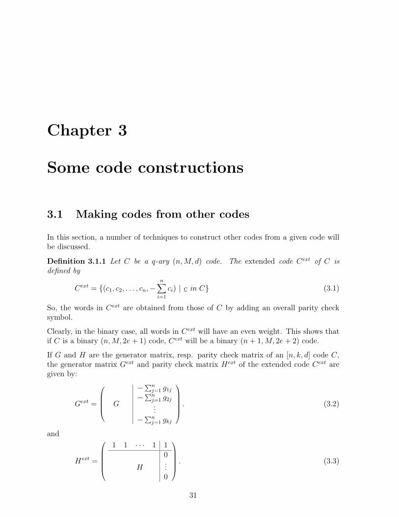
If G and H are the generator matrix, resp. parity check matrix of an [n, k, d] code C,the generator matrix Gext and parity check matrix Hext of the extended code Cext aregiven by:
Gext =
G
∣∣∣∣∣∣∣∣∣∣−∑n
j=1 g1j
−∑nj=1 g2j...
−∑nj=1 gkj
. (3.2)
and
Hext =
1 1 · · · 1 1
0
H...0
. (3.3)
31
CHAPTER 3. SOME CODE CONSTRUCTIONS
Two ways of making a code one symbol shorter are given in the following definition:
Definition 3.1.2 By puncturing a code on a specific coordinate, one simply deletes thatcoordinate in all codewords.
By shortening a code on a specific coordinate, say the j-th, with respect to symbol α,one takes only those codewords that have an α on coordinate j and then deletes that j-thcoordinate.
Let C be a q-ary (n,M, d) code. Then on each coordinate at least one symbol will occurat least dM/qe times. This proves the only non-trivial part in the next theorem.
Theorem 3.1.3 Let C be a q-ary (n,M, d) code with d ≥ 2. Then by puncturing acoordinate one obtains an (n− 1,M,≥ d− 1) code.
If C is a q-ary (n,M, d) code, one can shorten on any coordinate with respect to the mostfrequently occurring symbol on that coordinate to obtain an (n− 1,≥ dM/qe,≥ d) code.
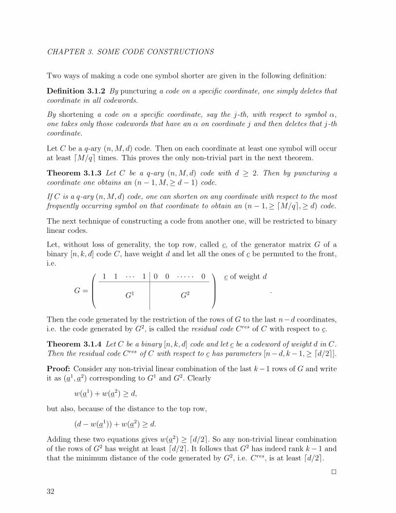
The next technique of constructing a code from another one, will be restricted to binarylinear codes.
Let, without loss of generality, the top row, called c, of the generator matrix G of abinary [n, k, d] code C, have weight d and let all the ones of c be permuted to the front,i.e.
G =
1 1 · · · 1 0 0 · · · · · 0
G1 G2
c of weight d
.
Then the code generated by the restriction of the rows of G to the last n−d coordinates,i.e. the code generated by G2, is called the residual code Cres of C with respect to c.
Theorem 3.1.4 Let C be a binary [n, k, d] code and let c be a codeword of weight d in C.Then the residual code Cres of C with respect to c has parameters [n− d, k− 1,≥ dd/2e].
Proof: Consider any non-trivial linear combination of the last k−1 rows of G and writeit as (a1, a2) corresponding to G1 and G2. Clearly
w(a1) + w(a2) ≥ d,
but also, because of the distance to the top row,
(d− w(a1)) + w(a2) ≥ d.
Adding these two equations gives w(a2) ≥ dd/2e. So any non-trivial linear combinationof the rows of G2 has weight at least dd/2e. It follows that G2 has indeed rank k− 1 andthat the minimum distance of the code generated by G2, i.e. Cres, is at least dd/2e.
2
32
3.1. MAKING CODES FROM OTHER CODES
As an example, consider the question of the existence of a binary [13, 6, 5] code. If itexisted, the residual code with respect to any minimum weight codeword would haveparameters [8, 5,≥ 3]. This however is impossible by the Hamming bound (Theorem2.1.3). So, no binary [13, 6, 5] code exists. It is however possible to construct a non-linear (13, 26, 5) code, but that construction will not be given here.
The above technique can easily be generalized to other fields than GF (2). One can alsodefine the residual code of C with respect to a codeword of weight more than d. Bothgeneralizations are left as an exercise to the reader.
The following corollary is a direct consequence of Theorem 3.1.4 and the fact that n′ ≥ d′
in a [n′, 1, d′] code.
Corollary 3.1.5 (The Griesmer bound) Let C be an [n, k, d] binary linear code.Then
n ≥k−1∑i=0
dd/2ie. (3.4)
The next construction will be needed in Section 3.3.
Theorem 3.1.6 ((u,u+v) construction) Let C1 be a binary (n,M1, d1) code and C2
a binary (n,M2, d2) code. Then the code C defined by
C = {(u, u+ v) | u in C1, v in C2} (3.5)
has parameters (2n,M1M2, d) with d = min{2d1, d2}.
If C1 and C2 are both linear, then so is C.
Proof: The length and cardinality of C are obvious. So the only thing left to check isthe minimum distance of C.
Let (u1, u1 + v1) and (u2, u2 + v2) be two distinct words in C. If v1 = v2, the distancebetween these two codewords is obviously equal to twice the distance between u1 andu2, so the distance is at least 2d1.
If v1 6= v2, then on each of the at least d2 coordinates where v1 and v2 differ, either alsou1 and u2 differ or u1 +v1 and u2 +v2 differ. So in this case (u1, u1 +v1) and (u2, u2 +v2)have distance at least d2.
The proof of the linearity of C in case that both C1 and C2 are linear is straightforward.
2
The next construction also makes use of two codes, but now over different fields.
Let C1 be a q-ary (n1,M1, d1) code and let C2 be a M1-ary (n2,M2, d2) code. Note thatthe alphabet size of code C2 is equal to M1, the cardinality of C1. So, one can replaceeach element in this alphabet of size M1 by a unique codeword in C1. Replacing eachcoordinate in the codewords of C2 by the corresponding vector in C1 results in a q-ary
33
CHAPTER 3. SOME CODE CONSTRUCTIONS
code that is called the concatenated code of the inner code C1 and the outer code C2.The following theorem is now obvious.
Theorem 3.1.7 (Concatenated code) Let C1 be a q-ary (n1,M1, d1) code and C2 bea M1-ary (n2,M2, d2) code. Then the concatenated code of the inner code C1 and outercode C2 is a q-ary code with parameters (n1n2,M2, d1d2).
3.2 The Hamming codes
Equation (2.14) can be interpreted as follows: a word c is a codeword in a linear code Cif and only if (abbreviated in the sequel to “iff”) the coordinates of c give a dependencyrelation between the the columns of the parity check matrix H of C.
In particular the minimum distance d of a linear code will satisfy d ≥ 2 iff H does notcontain the all-zero column. Similarly, d ≥ 3 iff H does not contain two columns thatare linearly dependent (the dual of such a code is sometimes called a projective code).In general, C will have minimum distance ≥ d iff each d − 1-tuple of columns in His linearly independent. If at least one d-tuple of columns is linearly dependent, theminimum distance will be exactly equal to d.
In view of the above, we now know that the length of a q-ary [n, k, 3] code is upperbounded by the maximum number of pairwise linearly independent vectors in Vr(q),where r = n − k is the redundancy of C. Now Vr(q) has qr − 1 non-zero vectors. Theycan be divided into (qr − 1)/(q − 1) groups of size q − 1, each consisting of a non-zerovector in Vr(q) together with all its non-zero scalar multiples. The extreme case thatn = (qr − 1)/(q − 1) leads to the following definition.
Definition 3.2.1 (Hamming code) The q-ary Hamming code oflength n = (qr − 1)/(q − 1) and redundancy r is defined by the parity check matrix thatconsists of (a maximum set of) columns that are all pairwise linearly independent.
It is denoted by Hr(q). The minimum distance of Hr(q) is equal to 3.
The reason for writing “the” Hamming code instead of “a” Hamming code simply is thatall q-ary Hamming codes of the same length are equivalent to each other.
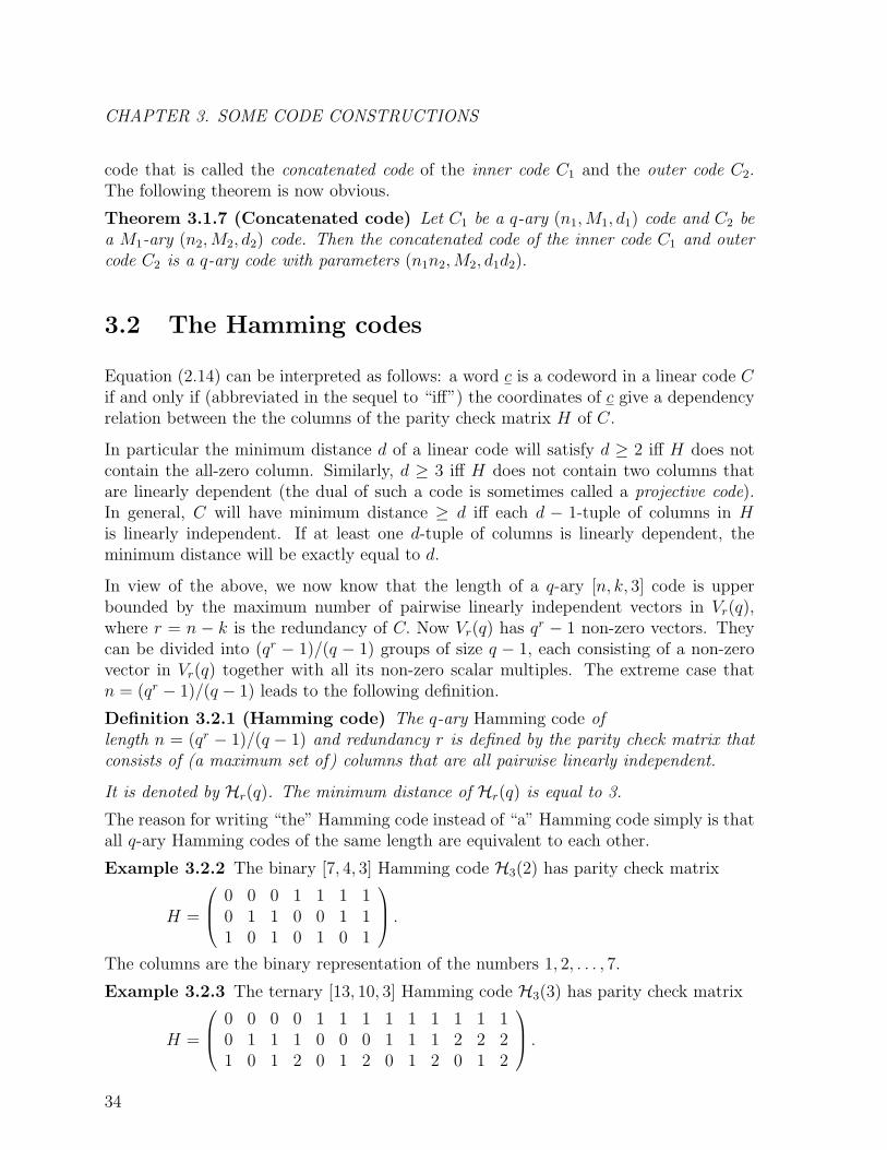
Example 3.2.2 The binary [7, 4, 3] Hamming code H3(2) has parity check matrix
H =
0 0 0 1 1 1 10 1 1 0 0 1 11 0 1 0 1 0 1
.The columns are the binary representation of the numbers 1, 2, . . . , 7.
Example 3.2.3 The ternary [13, 10, 3] Hamming code H3(3) has parity check matrix
H =
0 0 0 0 1 1 1 1 1 1 1 1 10 1 1 1 0 0 0 1 1 1 2 2 21 0 1 2 0 1 2 0 1 2 0 1 2
.34
3.2. THE HAMMING CODES
The examples above give a systematic way of making the parity check matrix of aHamming code: Take only the columns, whose first non-zero entry, when reading fromthe top to the bottom, is a 1.
Theorem 3.2.4 The q-ary [n = (qr − 1)/(q− 1), k = n− r, 3] Hamming code is perfect.
Proof: The volume of a sphere of radius 1 around a codeword is 1+n(q−1) = qr = qn−k.From
|C|qn−k = qkqn−k = qn
we have that equality holds in the Hamming bound (Theorem 2.1.3). So the coveringradius of the Hamming code is also 1. The statement now follows from Definition 2.1.6.
2
Decoding the Hamming code is extremely simple. Let r be a received word. Compute itssyndrome s = HrT . Definition 3.2.1 implies that s is the scalar multiple of some columnof the parity check matrix, say α times the j-th column. Now simply subtract α fromthe j-th coordinate to find the closest codeword. Indeed, the vector (r1, . . . , rj−1, rj −α, rj+1, . . . , rn) has syndrome 0.
The fact that a code is perfect implies that its weight enumerator is uniquely determinedby its parameters. We shall demonstrate this for the binary Hamming code.
Consider one of the(
nw
)words of weight w in Vn, say x. It is either a codeword in the
[n = 2r − 1, n− r, 3] Hamming code, or it lies at distance 1 from a unique codeword, sayfrom c. In the latter case, c has either weight w + 1 and x can be obtained from c byreplacing one of its w + 1 one-coordinates into a 0, or c has weight w − 1 and x can beobtained from c by replacing one of its n− (w− 1) zero-coordinates into a 1. Since eachof these coordinate changes yield different words of weight w (otherwise d = 3 cannothold), we have proved that the weight enumerator A(z) of the binary Hamming code oflength n = 2r − 1 satisfies the recurrence relation(
n
w
)= Aw + (w + 1)Aw+1 + (n− w + 1)Aw−1, 0 ≤ w ≤ n. (3.6)
With A0 = 1 and A1 = A2 = 0, one can now easily determine the whole weight enumer-ator recursively. For instance w = 2 yields
(n2
)= 3A3, i.e. A3 = n(n− 1)/6.
With the standard technique of solving recurrence relations one can find a closed expres-sion for A(z). It is however much easier to derive this with the MacWilliams relations.
The dual code of a Hamming code is called the Simplex code. In Examples 3.2.2 and 3.2.3one can see that all rows of the parity check matrices (thus of the generator matricesof the corresponding Simplex codes) have weight qr−1. This turns out to hold for allnon-zero codewords in the Simplex code.
35
CHAPTER 3. SOME CODE CONSTRUCTIONS
Theorem 3.2.5 All non-zero codewords in the Simplex code of length (qr − 1)/(q − 1)have weight qr−1, so the Simplex code has weight enumerator
A(z) = 1 + (qr − 1)zqr−1
. (3.7)
Proof: Suppose that the Simplex code has a codeword of weight w with w > qr−1, say c.Without loss of generality we may assume that the first w coordinates of c are non-zeroand that they all are equal to 1 (otherwise consider an equivalent Simplex code, whichwill have the same structure).
Use c as top row of a new generator matrix of this code. The first w (> qr−1) columns ofthis generator matrix all start with a 1 and are then followed by r− 1 other coordinates.However there are only qr−1 different q-ary (r − 1)-tuples, so at least two of the firstw > qr−1 columns are identical to each other. Since this generator matrix is also theparity check matrix of the Hamming code, we have a contradiction with Definition 3.2.1.
If the Simplex code of length (qr−1)/(q−1) has a codeword of weight w with w < qr−1,a similar contradiction can be obtained by considering the columns where this codewordhas its zero-coordinates.
2
The next theorem now immediately follows from the MacWilliams relations (Theorem2.3.4).
Theorem 3.2.6 The weight enumerator of the q-ary Hamming code of length n =(qr − 1)/(q − 1) is given by A(z) =
1qr
{(1 + (q − 1)z)n + (qr − 1)(1− z)qr−1
(1 + (q − 1)z)n−qr−1}.
(3.8)
3.3 Reed-Muller codes
The final class of linear codes in this chapter dates back to a paper by D.E. Muller in1954. In the same year I.S. Reed proposed a decoding algorithm for this code. Althoughthis class of codes can be generalized to other fields, we shall only discuss the binarycase.
In this section we consider binary polynomials f = f(x1, x2, . . . , xm) in m variables,where m is some fixed integer. Since only binary values will be substituted in f andx2 = x for x = 0 and 1, each variable will only occur to the power at most 1. Of courseterms like x2x4x5 can occur. If f contains a term which is the product of r variablesbut no term which is a product of ≥ r + 1 variables, f is said to have degree r. Clearly0 ≤ r ≤ m.
36
3.3. REED-MULLER CODES
Any polynomial f of degree ≤ r can be written as follows:
f(x1, x2, . . . , xm) =r∑
l=0
∑1≤i1<i2<···<il≤m
ai1i2···ilxi1xi2 · · ·xil , (3.9)
where a∅ denotes the constant term.
For example, 1 + x1 + x3 + x1x2 + x2x3x4 is a polynomial of degree 3.
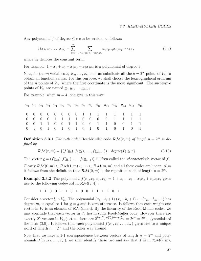
Now, for the m variables x1, x2, . . . , xm one can substitute all the n = 2m points of Vm toobtain all function values. For this purpose, we shall choose the lexicographical orderingof the n points of Vm, where the first coordinate is the most significant. The successivepoints of Vm are named u0, u1, . . . , un−1.
For example, when m = 4, one gets in this way:
u0 u1 u2 u3 u4 u5 u6 u7 u8 u9 u10 u11 u12 u13 u14 u15
0 0 0 0 0 0 0 0 1 1 1 1 1 1 1 10 0 0 0 1 1 1 1 0 0 0 0 1 1 1 10 0 1 1 0 0 1 1 0 0 1 1 0 0 1 10 1 0 1 0 1 0 1 0 1 0 1 0 1 0 1
Definition 3.3.1 The r-th order Reed-Muller code RM(r,m) of length n = 2m is de-fined by
RM(r,m) = {(f(u0), f(u1), . . . , f(un−1)) | degree(f) ≤ r}. (3.10)
The vector c = (f(u0), f(u1), . . . , f(un−1)) is often called the characteristic vector of f.
ClearlyRM(0,m) ⊂ RM(1,m) ⊂ · · · ⊂ RM(m,m) and all these codes are linear. Alsoit follows from the definition that RM(0,m) is the repetition code of length n = 2m.
Example 3.3.2 The polynomial f(x1, x2, x3, x4) = 1 + x1 + x3 + x1x2 + x2x3x4 givesrise to the following codeword in RM(3, 4) :
1 1 0 0 1 1 0 1 0 0 1 1 1 1 0 1
Consider a vector b in Vm. The polynomial (x1−b1 +1) (x2−b2 +1) · · · (xm−bm +1) hasdegree m, is equal to 1 for x = b and is zero otherwise. It follows that each weight-onevector in Vn is an element of RM(m,m). By the linearity of the Reed-Muller codes, wemay conclude that each vector in Vn lies in some Reed-Muller code. However there are
exactly 2n vectors in Vn, just as there are 21+(m1 )+(m
2 )+···+(mm) = 22m
= 2n polynomials ofthe form (3.9). It follows that each polynomial f(x1, x2, . . . , xm) gives rise to a uniqueword of length n = 2m and the other way around.
Now that we have a 1-1 correspondence between vectors of length n = 2m and poly-nomials f(x1, x2, . . . , xm), we shall identify these two and say that f is in RM(r,m),
37
CHAPTER 3. SOME CODE CONSTRUCTIONS
when f has degree less than or equal to r. Similarly we shall say that two polynomialsare orthogonal to each other, when we really mean that their characteristic vectors areorthogonal to each other.
The reasoning above also proves that the dimension of RM(r,m) is equal to the number
of choices of the coefficients in (3.9), i.e. 1 +(
m1
)+ · · ·+
(mr
).
Theorem 3.3.3 The r-th Reed-Muller code RM(r,m) of length n = 2m has parameters
[n,∑r
l=0
(ml
), 2m−r].
Proof: It remains to show that RM(r,m) has minimum distance 2m−r. That it cannotbe more follows from the fact that the polynomial x1x2 · · ·xr is in RM(r,m) and thatits function value is 1 iff x1 = x2 = . . . = xr = 1 (independent of values of xr+1, . . . , xm),so its weight is 2m−r.
That the minimum distance is at least 2m−r will follow with an induction argument fromTheorem 3.1.6. For m = 1, the statement is trivial.
By splitting the terms in a polynomial f(x1, x2, . . . , xm) in RM(r,m) into thosethat do contain x1 and those that do not, one can write f as p(x2, x3, . . . , xm) +x1q(x2, x3, . . . , xm), with p in RM(r,m − 1) and q in RM(r − 1,m − 1). Also eachchoice of p in RM(r,m − 1) and q in RM(r − 1,m − 1) gives rise to a unique f inRM(r,m).
Now p corresponds to a codeword u in RM(r,m−1), which by the induction hypothesishas minimum distance d1 = 2m−r−1. Similarly, q corresponds to a codeword v inRM(r−1,m− 1), with minimum distance d1 = 2m−r. Moreover p+ x1q has characteristic vector(u, u+ v).
It follows from the above that RM(r,m) is the result of the (u, u + v) constructionin Theorem 3.1.6 applied to C1 = RM(r,m − 1) and C2 = RM(r − 1,m − 1). Thesame theorem now says that RM(r,m) has minimum distance greater than or equal tomin{2d1, d2}= min{2 · 2m−r−1, 2m−r} = 2m−r.
2
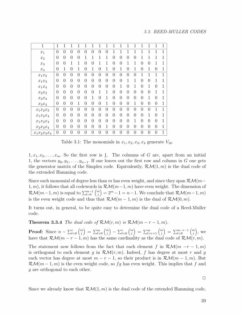
In Table 3.1 one can find the characteristic vectors of all possible terms in a polynomialin x1, x2, x3 and x4. They are listed in order of non-decreasing degree. As a result the toprow generates RM(0, 4), the top 1 +
(41
)rows generate RM(1, 4), etc. Note that row
x1x2 is just the coordinate-wise product of rows x1 and x2. The same holds for the otherhigher degree terms. This implies in particular, that the innerproduct of two monomialsis just the weight of their product. Since f(b) = g(b) = 1 if and only if (fg)(b) = 1, thesame is true for all polynomials: the innerproduct of two polynomials f and g is equalto the weight of their product fg.
The generator matrix G of RM(1,m) has as rows the characteristic vectors of
38
3.3. REED-MULLER CODES
1 1 1 1 1 1 1 1 1 1 1 1 1 1 1 1 1x1 0 0 0 0 0 0 0 0 1 1 1 1 1 1 1 1x2 0 0 0 0 1 1 1 1 0 0 0 0 1 1 1 1x3 0 0 1 1 0 0 1 1 0 0 1 1 0 0 1 1x4 0 1 0 1 0 1 0 1 0 1 0 1 0 1 0 1x1x2 0 0 0 0 0 0 0 0 0 0 0 0 1 1 1 1x1x3 0 0 0 0 0 0 0 0 0 0 1 1 0 0 1 1x1x4 0 0 0 0 0 0 0 0 0 1 0 1 0 1 0 1x2x3 0 0 0 0 0 0 1 1 0 0 0 0 0 0 1 1x2x4 0 0 0 0 0 1 0 1 0 0 0 0 0 1 0 1x3x4 0 0 0 1 0 0 0 1 0 0 0 1 0 0 0 1x1x2x3 0 0 0 0 0 0 0 0 0 0 0 0 0 0 1 1x1x2x4 0 0 0 0 0 0 0 0 0 0 0 0 0 1 0 1x1x3x4 0 0 0 0 0 0 0 0 0 0 0 1 0 0 0 1x2x3x4 0 0 0 0 0 0 0 1 0 0 0 0 0 0 0 1x1x2x3x4 0 0 0 0 0 0 0 0 0 0 0 0 0 0 0 1
Table 3.1: The monomials in x1, x2, x3, x4 generate V16.
1, x1, x2, . . . , xm. So the first row is 1. The columns of G are, apart from an initial1, the vectors u0, u1, . . . , un−1. If one leaves out the first row and column in G one getsthe generator matrix of the Simplex code. Equivalently, RM(1,m) is the dual code ofthe extended Hamming code.
Since each monomial of degree less thanm has even weight, and since they spanRM(m−1,m), it follows that all codewords inRM(m−1,m) have even weight. The dimension of
RM(m−1,m) is equal to∑m−1
l=0
(ml
)= 2m−1 = n−1. We conclude that RM(m−1,m)
is the even weight code and thus that RM(m− 1,m) is the dual of RM(0,m).
It turns out, in general, to be quite easy to determine the dual code of a Reed-Mullercode.
Theorem 3.3.4 The dual code of RM(r,m) is RM(m− r − 1,m).
Proof: Since n − ∑rl=0
(ml
)=∑m
l=0
(ml
)− ∑r
l=0
(ml
)=∑m
l=r+1
(ml
)=∑m−r−1
l=0
(ml
), we
have that RM(m− r − 1,m) has the same cardinality as the dual code of RM(r,m).
The statement now follows from the fact that each element f in RM(m −r − 1,m)is orthogonal to each element g in RM(r,m). Indeed, f has degree at most r and geach vector has degree at most m − r − 1, so their product is in RM(m − 1,m). ButRM(m− 1,m) is the even weight code, so fg has even weight. This implies that f andg are orthogonal to each other.
2
Since we already know that RM(1,m) is the dual code of the extended Hamming code,
39
CHAPTER 3. SOME CODE CONSTRUCTIONS
we now also know that RM(m− 2,m) is equal to the extended Hamming code.
The next property of Reed-Muller codes shows that they have even more internal struc-ture. In Chapter 2, two codes that could be obtained from each other by a coordinatepermutation and by alphabet permutations for each coordinate were called equivalent.To preserve linearity, for linear codes we do not allow all alphabet permutations but justthose that leave the finite field structure intact. For q = 2 this means that we only allowcoordinate permutations.
It turns out that some coordinate permutations combined with alphabet/field permu-tations, when applied to a code, yield the very same code. This means that the set ofcodewords is mapped in a 1-1 way to the set of codewords. Such permutations are calledautomorphisms of a code. The automorphisms of a code C form a group denoted byAut(C).
To describe a class of automorphisms of the Reed-Muller code of length n = 2m itwill prove to be useful to index the coordinates of the codewords c = (c0, c1, . . . , cn−1)with the vectors u0, u1, . . . , un−1 in Vm. An invertible, affine transformation of Vm i.e. amapping of the form x→ xA+b, where A is a non-singular m×m matrix and b is in Vm,obviously is a 1-1 mapping of Vm to Vm. So, an invertible, affine transformation of Vm
applied to the coordinates of the codewords of a Reed-Muller code yields an equivalentcode.
For instance, when m = 4 (n = 24 = 16) the coordinate transformation applied toc = (c0, c1, . . . , c15) given by
x1
x2
x3
x4
→
1 1 1 01 0 0 10 1 1 01 1 0 1
x1
x2
x3
x4
+
1001
maps (0, 0, 0, 0) to (1, 0, 0, 1) so c0 will appear at coordinate 9. Also (1, 0, 0, 0) will bemapped to (0, 1, 0, 0) and thus c8 will appear at coordinate 4. Etc.
The nice thing is that applying these invertible, affine transformations to a Reed-Mullercode will not just result in an equivalent code, but in the original code itself!
Theorem 3.3.5 The automorphism group Aut(RM(r,m)) of RM(r, m) contains thegroup of invertible, affine transformations of Vm.
Proof: Applying an invertible, affine transformations to a codeword f of degree at mostr, amounts to considering the word f(xA + b). Clearly f(xA + b) also has degree atmost r, since each variable xi in f is simply replaced by another linear expression (to beprecise by: ai1x1+ai2x2+ . . .+aimxm+bi). So f(xA+b) is also a codeword in RM(r,m).Since x → xA + b defined a permutation of the coordinates, it follows that it is indeedan automorphism of RM(r,m).
2
40
3.3. REED-MULLER CODES
The above theorem is a very important tool in the study of the weight structure ofReed-Muller codes, especially those of order 2. For instance the codeword
f(x1, x2, x3, x4) = x1x2 + x1x3 + x1x4 + x2x3 + x2 + x3 + 1
in RM(2, 4) can be rewritten as
(x1 + x3 + 1)(x2 + x3 + x4) + x3x4 + x3 + x4 + 1,
so it is equivalent under the invertible, affine transformation
x1 + x3 + 1 → x1
x2 + x3 + x4 → x2
x3 → x3
x4 → x4
to
x1x2 + x3x4 + x3 + x4 + 1.
This polynomial in turn can be rewritten as x1x2 + (x3 + 1)(x4 + 1), so it is equivalentto x1x2 + x3x4. Now, x1x2 + x3x4 is equal to 1 iff one of the terms is 1 and the other 0.It follows that x1x2 + x3x4 and thus f has weight 2 · 1 · 3 = 6.
We end this section by describing a decoding algorithm for the Reed-Muller code. SinceRM(r,m) has minimum distance 2m−r, we want to correct t errors for all t < 2m−r−1.
Consider the term xm−r+1xm−r+2 · · ·xm in a codeword f inRM(r,m) (see (3.9)). Clearlyit has innerproduct 1 with each of the 2m−r words (x1 + u1)(x2 + u2) · · · (xm−r + um−r).Indeed, there is only coordinate where both terms are equal to one, namely (u1 +1, u2 +1, . . . , um−r + 1, 1, 1, . . . , 1). Also, all other terms in f are orthogonal to (x1 + u1)(x2 +u2) · · · (xm−r +um−r), because their product (which will miss at least one of the variablesxi,m− r + 1 ≤ i ≤ m) is in RM(m− 1,m) and thus has even weight.
It follows that the coefficient am−r+1,m−r+2,···,m of xm−r+1xm−r+2 · · ·xm in a codeword fin RM(r,m) is equal to the innerproduct of f with each of the 2m−r words (x1+u1)(x2+u2) · · · (xm−r + um−r).
Let c be the characteristic vector of f . What we have shown above translates into the2m−r equations:
am−r+1,m−r+2,···,m = c0 + c1 + · · · + c2r−1.am−r+1,m−r+2,···,m = c2r + c2r+1 + · · · + c2.2r−1.
......
...am−r+1,m−r+2,···,m = c2m−2r + c2m−2r+1 + · · · + c2m−r.2r−1.
(3.11)
For instance, the choice of u1 = u2 = · · · = um−r = 1 will give the equation thatam−r+1,m−r+2,···,m is equal to the modulo 2 sum of those coordinates of c where x1 = x2 =· · · = xm−r = 0 i.e. coordinates 0, 1, . . . , 2r − 1.
41
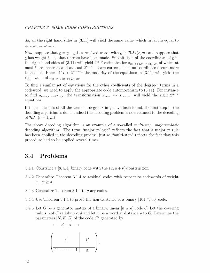
CHAPTER 3. SOME CODE CONSTRUCTIONS
So, all the right hand sides in (3.11) will yield the same value, which in fact is equal toam−r+1,m−r+2,···,m.
Now, suppose that r = c + e is a received word, with c in RM(r,m) and suppose thate has weight t, i.e. that t errors have been made. Substitution of the coordinates of r inthe right hand sides of (3.11) will yield 2m−r estimates for am−r+1,m−r+2,···,m of which atmost t are incorrect and at least 2m−r − t are correct, since no coordinate occurs morethan once. Hence, if t < 2m−r−1 the majority of the equations in (3.11) will yield theright value of am−r+1,m−r+2,···,m.
To find a similar set of equations for the other coefficients of the degree-r terms in acodeword, we need to apply the appropriate code automorphism to (3.11). For instanceto find am−r,m−r+2,···,m the transformation xm−r ↔ xm−r+1 will yield the right 2m−r
equations.
If the coefficients of all the terms of degree r in f have been found, the first step of thedecoding algorithm is done. Indeed the decoding problem is now reduced to the decodingof RM(r − 1,m)
The above decoding algorithm is an example of a so-called multi-step, majority-logicdecoding algorithm. The term “majority-logic” reflects the fact that a majority rulehas been applied in the decoding process, just as “multi-step” reflects the fact that thisprocedure had to be applied several times.
3.4 Problems
3.4.1 Construct a [8, 4, 4] binary code with the (u, u+ v)-construction.
3.4.2 Generalize Theorem 3.1.4 to residual codes with respect to codewords of weightw, w ≥ d.
3.4.3 Generalize Theorem 3.1.4 to q-ary codes.
3.4.4 Use Theorem 3.1.4 to prove the non-existence of a binary [101, 7, 50] code.
3.4.5 Let G be a generator matrix of a binary, linear [n, k, d] code C. Let the coveringradius ρ of C satisfy ρ < d and let x be a word at distance ρ to C. Determine theparameters [N,K,D] of the code C∗ generated by
← d− ρ →
0 G
1 · · · · · · 1 x
.
42
3.4. PROBLEMS
3.4.6 Let C∗ be an [n+ s, k + 1, d] code with generator matrix G∗. Suppose that somenon-zero column s in G∗ occurs s times with s < d.
Construct an [n, k, d] code with covering radius at least d− s.
3.4.7 Let x be a codeword of weight w in the dual code of a binary [n, k, d] code C.Shorten C with respect to the symbol 0 on all the coordinates where x is 1.
Prove that one obtains an [n− w,≥ k − w + 1,≥ d] code.
3.4.8 Give the weight enumerator A(z) of the binary Hamming code of length 31. Com-pute Ai
(31i )/25
for i = 5, 10 and 15.
3.4.9 Derive a recurrence relation for the weight enumerator of a binary (23, 212, 7) codeand a ternary (11, 36, 5) code containing the all-zero vector (hint: first show thatthese codes are perfect).
3.4.10 Use the preceding problem to argue that puncturing a binary evenweight [24, 12, 8]code on each of its coordinates results in [23, 12, 7] codes which all have the sameweight enumerators.
Prove that this property implies that in this punctured code the number of code-words of weight 2i− 1 and that of weight 2i are related, 0 ≤ i ≤ 12. What is thisrelation?
Derive the weight enumerator of the [23, 12, 7] code, obtained by puncturing a[24, 12, 8] code with weight enumerator 1 + 759z8 + 2576z12 + 759z16 + z24.
3.4.11 Suppose that a (90, 278, 5) binary code C exists. Prove that C has to be perfect.
Derive a recurrence relation for the weight enumerator A(z) of C.
Without loss of generality one may assume that C contains 0. Why? DetermineA0, A1, . . . , A7. Why should these numbers be integers and what is your conclusionabout the existence of C?
3.4.12 Prove that the Boolean function
∑1≤i<j≤m
aijxixj +∑
1≤i≤m
bixi + c
can be mapped into the the Boolean function
x1x2 +∑
3≤i<j≤m a′ijxixj +
∑3≤i≤m b
′ixi + c′ (∗)
by an invertible affine transformation x→Ux + u (i.e. U is invertible) as long asat least one of the aij’s is not equal to 0.
Which standard forms can be obtained for the elements ofRM(2, m) if one applies(∗) repeatedly?
43
CHAPTER 3. SOME CODE CONSTRUCTIONS
Which weights do occur in RM(2, 5)?
Show that RM(2, 5) is a selfdual code. Describe an easy way to find the weightenumerator of RM(2, 5) (the actual calculations do not have to be made).
3.4.13 Let c = a∅ +∑
1≤i≤5 aixi +∑
1≤i<j≤5 ai,jxixj be a codeword in RM(2, 5) and letr = c+ e with w(e) ≤ 3.
Write down 8 parity check equations that can be used (by a majority decodingtechnique) to determine
a1,3.
Write down 16 parity check equations that can be used to determine
a3
in c′ = c−∑1≤i<j≤5 ai,jxixj.
Write down 32 parity check equations that can be used to determine
a∅
in c′′ = c′ −∑1≤i≤5 aixi.
44
Chapter 4
Cyclic codes and Goppa codes
4.1 Introduction; equivalent descriptions
In Theorem 3.3.5 it was proved that certain coordinate permutations do map the codeonto itself. By assuming such internal structure, it may be easier to find good codes. Inthis chapter we shall study linear codes that are invariant under a cyclic shift.
This cyclic structure makes these codes quite easy to implement with simple logicalcircuits.
Definition 4.1.1 A code C is called cyclic if it is linear and for each (c0, c1, c2, . . . , cn−1)in C also (cn−1, c0, c1, . . . , cn−2) is in C.
The Hamming code of length seven in Example 3.2.2 is equivalent to the code C withparity check matrix:
H =
1 0 0 1 0 1 10 1 0 1 1 1 00 0 1 0 1 1 1
. (4.1)
One can easily check this by observing that the columns of the paritycheck matrices ofboth codes are a permutation of each other.
It is also a small effort to check that the non-zero codewords in C⊥ consist of the sevencyclic shifts of the top row in H.
It follows that if some vector is orthogonal to all words in C⊥, so are all its cyclic shifts.So also C is a cyclic code. Indeed it consists of 0, 1 and all the cyclic shifts of the vectors( 1 1 0 1 0 0 0 ) and ( 1 1 1 0 0 1 0 ).
The reader may already have noticed that the coordinates in Definition 4.1.1 are num-bered from 0 to n− 1. The reason is that powerful algebraic tools will be available, once
45
CHAPTER 4. CYCLIC CODES AND GOPPA CODES
we have identified the words in Vn(q) with q-ary polynomials over GF (q) in the followingway:
(c0, c1, c2, . . . , cn−1) ↔ c0 + c1x+ . . .+ cn−1xn−1. (4.2)
So, instead of writing c is in C, we shall often write c(x) is in C.
Notice that multiplying c(x) with x almost gives the polynomial corresponding to thecyclic shift of c. To really get this cyclic shift, one has to reduce xc(x) modulo xn − 1,i.e. replace xc(x) by its remainder after division by xn − 1. Indeed:
xc(x) ≡ x(c0 + c1x+ . . .+ cn−1xn−1) ≡
≡ c0x+ c1x2 + . . .+ cn−2x
n−1 + cn−1xn ≡
≡ cn−1 + c0x+ c1x2 + . . .+ cn−2x
n−1 (mod xn − 1).
So, instead of considering the set of all q-ary polynomials in x, usually denoted byGF (q)[x], we only work with the set of the residues of these polynomials modulo xn− 1.This new set is denoted by GF (q)[x]/(xn − 1), to suggest the division by xn − 1.
We conclude that a cyclic shift in Vn(q) corresponds to a multiplication by x inGF (q)[x]/(xn − 1). Of course, there is no reason to limit us to multiplications by x.Multiplication with any polynomial is now possible; just divide the product by xn − 1and take the remainder. The mathematical terminology for this is: GF (q)[x]/(xn − 1)is a ring.
Since a cyclic code is linear by definition, with c(x) in a cyclic code C, not only xc(x)is in C, but also x2c(x), x3c(x), etc., and all their linear combinations as well. In short,each multiple u(x)c(x) (mod xn − 1) is in C.
The next theorem shows that a cyclic code in Vn(q) can be described by a single poly-nomial in GF (q)[x]/(xn − 1).
Theorem 4.1.2 Let C be a cyclic code in Vn(q). Then there exists a unique monicpolynomial g(x) over GF (q) dividing xn − 1 with the property
c(x) is in C iff g(x) divides c(x). (4.3)
The polynomial g(x) is called the generator polynomial of C.
Proof: Let g(x) be the monic polynomial of lowest degree among the non-zero ele-ments in C. We have already seen that all polynomial-multiples u(x)g(x) of g(x) withdegree(u(x)) + degree(g(x)) < n are also in C.
It remains to show that any codeword c(x) in C, and thus also xn− 1 which is 0 moduloxn − 1, is a multiple of this g(x).
Divide c(x) by g(x), so write c(x) = u(x)g(x)+r(x), where degree(r(x)) < degree(g(x)).With g(x) in C, also u(x)g(x) is in C. Since c(x) is in C too, the linearity of C implies
46
4.1. INTRODUCTION; EQUIVALENT DESCRIPTIONS
that also r(x) is in the code C. But g(x) is the monic polynomial of lowest degree amongall the non-zero elements in C. We conclude that r(x) = 0 and thus that c(x) = u(x)g(x).
2
In GF (q)[x]/(xn − 1) there are more polynomials with property (4.3). See, for instance,Problem 4.6.8. Only g(x) has the additional property that it divides xn − 1.
The factorization of x7 − 1 over GF (2) into irreducible factors is given by
x7 − 1 = (x+ 1)(x3 + x+ 1)(x3 + x2 + 1).
The cyclic [7, 4, 3] Hamming code, at the beginning of this section has generator poly-nomial x3 + x+ 1.
The cyclic [7, 6, 2] even weight code has generator polynomial x+ 1.
The cyclic [7, 1, 7] repetition code has generator polynomial (x3 + x+ 1)(x3 + x2 + 1) =x6 + x5 + x4 + x3 + x2 + x+ 1.
Since x7 − 1 has three irreducible factors over GF (2) there are 23 distinct, binary cycliccodes of length 7. Some of these are equivalent.
Theorem 4.1.3 Let C be a k-dimensional, cyclic code in Vn(q) with generator polyno-mial g(x). Then the degree of g(x) is equal to n− k.
Write g(x) = g0 + g1x+ . . .+ gn−kxn−k. Then a generator matrix G for C is given by:
G =
g0 g1 · · · · · · gn−k 0 0 · · · 00 g0 g1 · · · · · · gn−k 0 · · · 00 0 g0 g1 · · · · · · gn−k · · · 0...
. . . . . . . . ....
0 0 · · · 0 g0 g1 · · · · · · gn−k
. (4.4)
Proof: Let the degree of g(x) be l. Then the (n − l) × n matrix G∗ with as rows thecodewords xig(x), 0 ≤ i < n− l, has rank n− l, because g(x) is monic.
Since each codeword must be divisible by g(x), it can be written as u(x)g(x). But eachcodeword also has degree less than n, so it can be written as u(x)g(x) with degree u(x)less than n− l. In other words, each codeword is a linear combination of the rows of G∗.Since C has dimension k, we conclude that k = n− l and that G∗ = G.
2
To encode information sequence a(x) = a0 + a1x + . . . + ak−1xk−1 one can of course
multiply G by (a0, a1, . . . , ak−1), but a faster way is by means of the alternativegenerator matrix G′ = (PIn−k), that can easily be obtained from G by elemen-tary row operations. Compute a(x)xn−k and divide the result by g(x). Let r(x) bethe remainder (of degree less than n − k), so r(x) ≡ a(x)xn−k (mod g(x).) Then
47

CHAPTER 4. CYCLIC CODES AND GOPPA CODES
c = (−r0,−r1, · · · ,−rn−k−1, a0, a1, · · · , ak−1) is the encoding of a(x). Indeed, c(x) =−r(x) + a(x)xn−k ≡ −r(x) + r(x) ≡ 0 (mod g(x)) and this c(x) obviously is the encod-ing of a(x) by means of G′.
From Theorem 4.1.2 we know that the generator polynomial g(x) of a cyclic code Cin Vn(q) must divide xn − 1. Let h(x) be the quotient, so let xn − 1 = g(x)h(x). Thispolynomial h(x) gives an alternative way to describe cyclic codes.
Theorem 4.1.4 Let C be a cyclic code in Vn(q) with generator polynomial g(x). Leth(x) = (xn − 1)/g(x). Then, in GF (q)[x]/(xn − 1),
c(x) is in C iff c(x)h(x) = 0. (4.5)
The polynomial h(x) is called the parity check polynomial of C.
Proof: ⇒ If c(x) is in C it can be written as a(x)g(x). So c(x)h(x) = a(x)g(x)h(x) =a(x)(xn − 1) = 0 in GF (q)[x]/(xn − 1).
⇐ If c(x)h(x) = 0 in GF (q)[x]/(xn−1) one has that xn−1 divides c(x)h(x), i.e. g(x)h(x)divides c(x)h(x) and thus that g(x) divides c(x).
2
Since xn − 1 ≡ 0 (mod xn − 1), comparing the coefficient of xl, 0 ≤ l < n, in both sidesof g(x)h(x) ≡ 0 (mod xn − 1) will give the following equation:
n−1∑i=0
gihl−i = 0,
where the indices have to be taken modulo n. In this summation, the terms 0 ≤ i ≤ lgive the coefficient of xl in g(x)h(x) and the terms l + 1 ≤ i < n give the coefficient ofxl+n in g(x)h(x), which reduces to xl modulo xn − 1.
It follows (by taking l = i+ j) that each shift (gi, gi+1, . . . , gn−1, g0, . . . , gi−1), 0 ≤ i < n,of g(x) is orthogonal to each vector (hj, hj−1, . . . , h0, hn−1 . . . , hj+1), 0 ≤ j < n. Let Chave dimension k, so g(x) has degree n−k and h(x) has degree k. Then, the above showsthat C has the following parity check matrix:
H =
0 · · · 0 0 hk · · · · · · h1 h0
0 · · · 0 hk · · · · · · h1 h0 0... · · · ...... · · · ...hk · · · · · · h1 h0 0 · · · 0 0
. (4.6)
The matrix H above also generates a cyclic code. The generator polynomial of this code(which is C⊥) is 1
h0(hk + hk−1x+ · · ·+ h1x
k−1 + h0xk) = 1
h0xkh(1/x).
We conclude that the dual code of a cyclic code in Vn(q), with generator polynomialg(x), is also cyclic with generator polynomial xkh(1/x), where xn − 1 = g(x)h(x). This
48

4.1. INTRODUCTION; EQUIVALENT DESCRIPTIONS
dual code is equivalent to the cyclic code generated by h(x) (just take all columns inreverse order).
To be able to say something about the minimum distance of cyclic codes, it will benecessary to consider an extension field of GF (q) in which xn−1 factors completely intolinear factors.
Consider for instance GF (8). It can be viewed as GF (2)[x]/(x3 + x + 1), i.e. the set ofbinary polynomials in x reduced modulo the irreducible polynomial x3 + x + 1. Equiv-alently, let α be a zero of x3 + x + 1, so α3 = 1 + α. Then GF (8) has the binarypolynomials of degree at most 2 in α as its elements. For the multiplication, oneshould use the relation α3 = 1 + α to reduce the degree to less than 3. For exam-ple (1+α2)2 = 1+α4 = α(α3 +α+1)+α2 +α+1 = α2 +α+1. As a matter of fact α is,in this example, a generator of the multiplicative group of GF (2)[x]/(x3 + x+ 1). Thatis why α is called a primitive element of GF (8) and why x3 + x+ 1 is called a primitivepolynomial.
Now note that the columns in matrix (4.1) are exactly the elements 1, α, . . . , α6, writtenas polynomials of degree at most 2 in α. So, the binary, cyclic Hamming code of length7 can be described in terms of the non-binary (!) parity check matrix
H =(
1 α α2 α3 α4 α5 α6)
(4.7)
i.e. as the code {c in C | HcT = 0T}. This cyclic code has generator polynomial g(x) =1 + x + x3, which factors into (x − α)(x − α2)(x − α4) over GF (23), and parity checkpolynomial h(x) = (1+x)(1+x2 +x3), which factors into (x−1)(x−α3)(x−α5)(x−α6)over GF (23).
This follows from the factorization of x7 − 1 in GF (2)[x]
x7 − 1 = (1 + x)(1 + x+ x3)(1 + x2 + x3)
and the factorization of x7 − 1 over GF (23)
x7 − 1 = (x− 1)(x− α) · · · (x− α6).
So, one has
x7 − 1
1 + x+ x3= (1 + x)(1 + x2 + x3),
as well as
x7 − 1
(x− α)(x− α2)(x− α4)= (x− 1)(x− α3)(x− α5)(x− α6).
In general
xqm−1 − 1 =∏
ξ∈GF (qm), ξ 6=0
(x− ξ).
So, one can get a complete factorization of xn − 1 into linear factors over GF (qm), ifn|(qm−1), or equivalently qm ≡ 1 (mod n). Indeed, let n|(qm−1) and let ω be a primitive
49
CHAPTER 4. CYCLIC CODES AND GOPPA CODES
element in GF (qm). Then the n different powers of α = ω(qm−1)/n will all be a zero ofxn − 1 and thus
xn − 1 =n−1∏i=0
(x− αi).
Since α is a zero of xn − 1 and also generates the other zeros of xn − 1, it is called aprimitive n-th root of unity.
For the existence of an integer m such that qm ≡ 1 (mod n) it is necessary and sufficientto assume that the gcd of q and n is equal to 1. From now on, we shall always assumethat. In particular, binary cyclic codes will always have odd length.
It also follows from the above that the generator polynomial g(x) of a cyclic code C inVn(q) can be written as
g(x) =∏i∈I
(x− αi), (4.8)
where I is a subset of {0, 1, . . . , n−1}, called the defining set of C with respect to α. Theparity check polynomial h(x) has the complement of I in {0, 1, . . . , n − 1} as definingset.
In the notation of above, let f(x) be an irreducible q-ary polynomial dividing xn−1 andlet αi be a zero of f(x). From the theory of finite fields we know, that also (αi)q = αiq
is a zero of f(x) and by induction also αiq2, . . . , αiqm−1
(not all these elements have tobe different). Of course these exponents can be reduced modulo n, since αn = 1. Theelements αiqj
are called the conjugates of αi. The set {iqj | j = 0, 1, . . .} consisting ofthe exponents modulo n of these conjugates is called the cyclotomic coset Ci of i modulon.
The set of all conjugates of a zero αi of an irreducible polynomial f(x) gives the completefactorization of f(x) into linear factors:
f(x) =∏l∈Ci
(x− αl).
This polynomial f(x) is called the minimal polynomial of αi and is often denoted bymi(x).
What we have shown above is that a generator polynomial of a cyclic code is the productof some minimal polynomials and that the defining set of a cyclic code is the union ofthe corresponding cyclotomic cosets. A necessary and sufficient condition for this is thatthe defining set I has the property
i ∈ I ⇒ qi ∈ I,
where qi of course has to be reduced modulo n.
Example 4.1.5 Let q = 3 and n = 11. To find the smallest extension field of GF (3) thatcontains the 11-th roots of unity, one has to determine (the smallest) m with 11|(qm−1).
50

4.1. INTRODUCTION; EQUIVALENT DESCRIPTIONS
One obtains m = 5. So x11 − 1 =∏n−1
i=0 (x − αi), where α = ω(35−1)/11 for some (each)primitive element ω in GF (35).
There are three cyclotomic cosets. The first is C0 = 0, giving rise to the ternary polyno-mial m0(x) = x− 1. The other two are
C1 = {1, 3, 9, 5, 4}
and
C−1 = {2, 6, 7, 10, 8}.They give rise to the irreducible, ternary polynomials
m1(x) = (x− α)(x− α3)(x− α9)(x− α5)(x− α4) =
= x5 + x4 − x3 + x2 − 1
and
m−1(x) = (x− α2)(x− α6)(x− α7)(x− α10)(x− α8) =
= x5 − x3 + x2 − x− 1
(or the other way around depending on the choice of α).
The code generated by m1(x) (or by m−1(x)) has dimension k = 6.
The code in Example 4.1.5 will be studied further in Section 4.3.
In view of the above, it is not necessary to give the whole defining set I of a cycliccode, but just one element from each cyclotomic coset in the defining set. The otherelements (corresponding to the conjugates of these elements) have to be there anyhow.For instance, it is enough to say that the code in Example 4.1.5 generated by m1(x) hasdefining set {1}.
We summarize the preceding theory in the following theorem.
Theorem 4.1.6 Consider Vn(q) with gcd(q, n) = 1. Let m satisfy qm ≡ 1 (mod n) andlet ω be a primitive element in GF (qm). Then α = ω(qm−1)/n is a primitive n-th root ofunity.
Let I = {i1, i2, . . . , il} be a subset of {0, 1, . . . , n − 1}. Then I is the defining set of aq-ary, cyclic code C of length n and each cyclic code can be defined by such sets.
Let mi(x) be the minimal polynomial of αi. Then C can be described in the followingways:
C = {c(x) | mi(x) divides c(x) for all i in I}, (4.9)
C = {c(x) | c(αi) = 0 for all i in I}, (4.10)
C = {c ∈ Vn(q) | HcT = 0T}, (4.11)
51
CHAPTER 4. CYCLIC CODES AND GOPPA CODES
where
H =
1 αi1 α2i1 · · · · · · α(n−1)i1
1 αi2 α2i2 · · · · · · α(n−1)i2
......
...1 αil α2il · · · · · · α(n−1)il
.
One example of this theorem we have already seen. The binary Hamming code of length7 with parity check matrix (4.1) is a cyclic code with generator polynomial m1(x) =1 + x+ x3 which has α (and its conjugates) as zero. An equivalent parity check matrixis given in (4.7).
4.2 BCH codes and Reed-Solomon codes
In (4.7) we have seen that the binary Hamming code of length 7 is (equivalent to) acyclic code. This turns out to be true for all binary Hamming codes (to extend thisresult to other fields one has to be a little bit more careful).
Theorem 4.2.1 Let α be a primitive element in GF (2m). Then the binary, cyclic codeC of length n = 2m − 1 with defining set {1} has parameters [n = 2m − 1, n −m, 3], soit is a binary Hamming code.
Proof: Theorem 4.1.6 gives the 1×n parity check matrix (in GF (2m)) of the code withdefining set {1}. Since α is a primitive element of GF (2m) (and thus a primitive n-throot of unity) all the columns in H, when written as binary vectors, are distinct non-zerovectors in Vm.
This proves that C is the binary Hamming code of length 2m − 1.
2
The defining set {1} in Theorem 4.2.1 gives a binary code that is 1-error-correcting, soone may want to try {1, 2} as defining set for a 2-error-correcting, binary code. Thisdoes not work however, because c(α) = 0 implies (for binary c(x)) that c(α2) = 0, andthus this equation will not give any additional relation.
Theorem 4.2.2 Let α be a primitive element in GF (2m). The binary cyclic code C oflength n = 2m − 1 with defining set {1, 3} is 2-error correcting.
Instead of giving a proof that the code C in Theorem 4.2.2 has minimum distance 5, weshall give an algorithm for decoding up to 2 errors.
The parity check matrix of C is given by:
H =
(1 α1 α2 · · · · · · α(n−1)
1 α3 α2·3 · · · · · · α(n−1)·3
)
52
4.2. BCH CODES AND REED-SOLOMON CODES
Let c be the transmitted word and r the received word. So r = c+ e, where e has weightat most 2. The syndrome of r consists of the elements s1, s3 in GF (2m), defined by
s1 = r(α) = c(α) + e(α) = e(α),
s3 = r(α3) = c(α3) + e(α3) = e(α3),
where we have used the conditions on c in C : c(α) = c(α3) = 0.
There are three cases to be considered:
Case 0: w(e) = 0.
In this case r = c and no errors have been made. Further s1 = s3 = 0.
Case 1: w(e) = 1.
Let the single error be at coordinate i, so e(x) = xi. One has s1 = e(α) = αi ands3 = e(α3) = α3i. In particular, s3 = s3
1 and s1 6= 0.
Case 2: w(e) = 2.
Let the two errors be at coordinates i and j, so e(x) = xi + xj, i 6= j. One has s1 =e(α) = αi + αj and s3 = e(α3) = α3i + α3j.
Note that s3 + s31 = α3i + α3j + (αi + αj)3 = α2iαj + αiα2j = αi+j(αi + αj) = αi+js1.
Since i 6= j, in this case s3 6= s31.
It also follows that
x2 + s1x+s3 + s3
1
s1
= x2 + (αi + αj)x+ αi+j = (x− αi)(x− αj).
So the zeros of x2 + s1x+s3+s3
1
s1will give the locations of the errors.
Together, these three cases prove that the following algorithm will decode up to twoerrors.
Algorithm 4.2.3 Consider the binary, cyclic 2-error-correcting code of length n = 2m−1 of Theorem 4.2.2. Let r be a received word, which is at distance at most 2 from acodeword.
Then the closest codeword to r can be found in the following way:
• Determine the syndrome s1 = r(α) and s3 = r(α3).
• There are three mutually excluding cases:
1. If s1 = s3 = 0, the received word r is a codeword.
2. If s3 = s31 6= 0, a single error has been made at coordinate i, determined by
s1 = αi.
53

CHAPTER 4. CYCLIC CODES AND GOPPA CODES
3. If s3 6= s31, two errors have been made. Their coordinates i and j are deter-
mined by the zeros αi and αj of z2 + s1z +s3+s3
1
s1.
We shall now describe a very general class of cyclic codes with certain guaranteed min-imum distance properties. They are named after R.C. Bose, D.K. Ray-Chaudhuri andA. Hocquenghem (the first two found this class independently of the last).
Definition 4.2.4 Let α be a primitive n-th root of unity in an extension field of GF (q)and let I be the defining set of a q-ary cyclic code C of length n.
If I contains dBCH − 1 consecutive integers (taken modulo n), one says that C is a BCHcode of designed distance dBCH .
If I contains {1, 2, . . . , dBCH − 1} as a subset, the code C will be called a narrow-senseBCH code.
If n = qm − 1, the code C is called a primitive BCH code (in this case α itself is aprimitive field element).
The justification of the notation dBCH will be given in the following theorem.
Theorem 4.2.5 (BCH bound) The minimum distance d of a BCH code with designeddistance dBCH satisfies
d ≥ dBCH . (4.12)
Proof: We shall only prove the theorem for the special case of narrow-sense codes. Thegeneral case will follow from a theorem in the next section.
Take any non-zero codeword c(x) in C and compute the polynomial
C(X) =n∑
i=1
c(αi)Xn−i.
The polynomial C(X) is called the Mattson-Solomon polynomial of c(x). Because c(αi) =0 for 1 ≤ i ≤ dBCH − 1 by assumption, we conclude that C(X) is a polynomial in X ofdegree at most n− dBCH , so it has at most n− dBCH distinct zeros.
Now, for 0 ≤ l ≤ n− 1,
C(αl) =n∑
i=1
c(αi)α−il =n∑
i=1
n−1∑j=0
cjαijα−il =
=n−1∑j=0
n∑i=1
cjαi(j−l) = ncl,
because 1 + αu + α2u + . . . + α(nu−1)u for 1 ≤ u < n is equal to αn−1
αu−1which is zero. It
follows that at most n− dBCH coordinates cl can be zero and thus that c(x) has weightat least dBCH .
54
4.2. BCH CODES AND REED-SOLOMON CODES
2
How to decode up to eBCH = b(dBCH − 1)/2c errors is an entirely different problem.This will be discussed in a more general setting in Section 4.5.
Example 4.2.6 In order to construct a binary, narrow-sense BCH code of length 15with designed distance 7, one has to take a defining set including {1, 2, . . . , 6}. Clearly,GF (24) is the smallest extension field of GF (2) containing primitive 15-th roots of unity.
The relevant cyclotomic cosets in GF (24) are {1, 2, 4, 8}, {3, 6, 12, 9} and {5, 10}, withcorresponding irreducible polynomials m1(x), m3(x) and m5(x) of degree 4, 4, and 2respectively.
So, the binary cyclic code of length 15 generated by the 10-th degree polynomial g(x) =m1(x)m3(x)m5(x) has parameters [15, 5,≥ 7].
Example 4.2.7 Consider the binary code of length 23 with defining set {1} and let αbe a primitive 23-rd root of unity. One can find α in GF (211).
The cyclotomic coset of α1 is given by {1, 2, 4, 8, 16, 9, 18, 13, 3, 6, 12} of cardinality 11.In particular it contains 1, 2, 3 and 4. By the BCH bound this code has parameters[23, 12,≥ 5].
The actual minimum distance of the code in Example 4.2.7 will be determined in Section4.3.
The following special subclass of BCH codes turns out to be very important in manyapplications.
Definition 4.2.8 A Reed-Solomon code is a narrow-sense q-ary BCH code of lengthn = q − 1.
The smallest extension field of GF (q) containing n-th roots of unity with n = q −1 is of course GF (q) itself. Let α be a primitive element of GF (q). The generatorpolynomial g(x) of the Reed-Solomon code with designed minimum distance dBCH isgiven by
∏dBCH−1i=1 (x − αi), which has degree dBCH − 1. So this code has parameters
[n = q − 1, n − (dBCH − 1),≥ dBCH ]. It follows however from the linear version ofthe Singleton bound at the end of Section 2.2 that equality must hold, i.e. the actualminimum distance is equal to dBCH . A different way to see this is to observe that g(x)has degree dBCH−1 and thus weight at most dBCH . It follows that the minimum distanceof this Reed-Solomon code is also bounded above by dBCH and thus it must be equal todBCH .
So, Reed-Solomon codes are MDS. Shortening a MDS code again gives a MDS code.Thus, we have proved the first statement in the next theorem.
Theorem 4.2.9 The (shortened) Reed-Solomon codes are MDS. Also, the extendedReed-Solomon code is MDS.
55
CHAPTER 4. CYCLIC CODES AND GOPPA CODES
Proof: The extended code is defined by (3.1.1). A codeword c(x) of weight d cannotsatisfy c(1) = 0, because then it would have d consecutive zeros and by the BCH boundit would have weight at least d + 1. So c(1) 6= 0 and thus the extension of a weight dcodeword will have weight d+ 1.
2
4.3 The Golay codes
In this section we want to further analyze two codes that we have already seen before.The first one is the binary [23, 12,≥ 5] code C described in Example 4.2.7.
By looking at the cyclotomic coset containing α one sees that x23 − 1 = (x −1)m1(x)m−1(x) and that m1(x) = x11m−1(1/x).
Now consider a codeword c(x) in C of even weight w, say c(x) = xi1 + xi2 + · · ·+ xiw . Itfollows that
c(x) ≡ 0 (mod (x− 1)m1(x))
and, for the same reason, that
x23c(1/x) ≡w∑
u=1
x−iu ≡ 0 (mod (x− 1)m−1(x)).
Since x23 − 1 = (x− 1)m1(x)m−1(x), it follows that c(x)x23c(1/x) ≡0 (mod x23 − 1) and thus, because w is even,
0 ≡w∑
u=1
xiuw∑
v=1
x−iv ≡w∑
u 6=v,u,v=1
xiu−iv (mod x23 − 1).
Writing∑22
i=1 sixi for this sum, we conclude that each si must be zero modulo 2. However,
the sum also does not change under the mapping x→ 1/x modulo x23− 1, which showsthat si = s23−i.
The expression∑w
u 6=v,u,v=1 xiu−iv contains w(w−1) terms. Whenever there is a cancelation
of terms, say iu − iv ≡ iu′ − iv′ (mod 23), also a second cancelation of terms occurs:iv− iu ≡ iv′− iu′ (mod 23). So terms disappear four at a time. It follows that w(w−1) ≡ 0(mod 4). A different way of saying the same is: w(w − 1) ≡ ∑22
i=1 si ≡∑11
i=1 2si ≡0 (mod 4), since each si is even.
Since 2(2− 1) ≡ 2 (mod 4), we can conclude that no codewords in C occur of weight 2mod 4.
The code C obviously contains the all-one vector because∑22
i=0 xi = (x23 − 1)/(x− 1) =
m1(x)m−1(x). Let A(z) be the weight enumerator of C. From Ai = A23−i for all i, wenow know: A5 = A18 = 0, A6 = 0, proving that C has minimum distance at least 7.
56
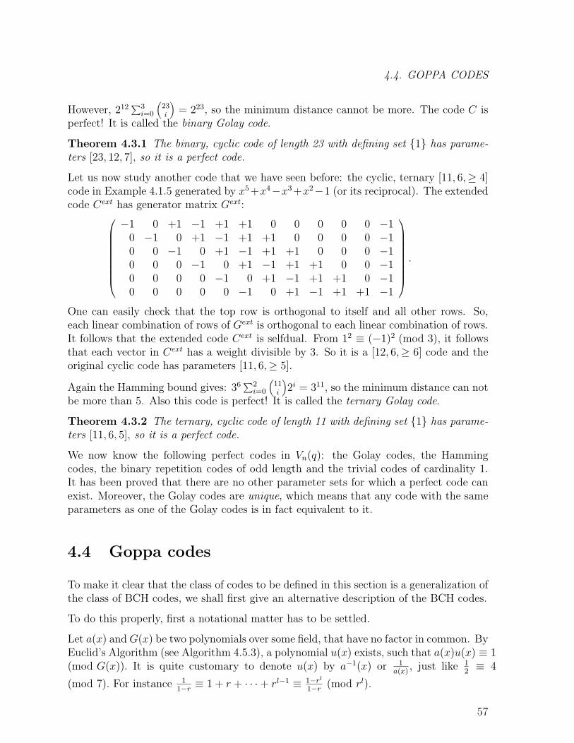
4.4. GOPPA CODES
However, 212∑3i=0
(23i
)= 223, so the minimum distance cannot be more. The code C is
perfect! It is called the binary Golay code.
Theorem 4.3.1 The binary, cyclic code of length 23 with defining set {1} has parame-ters [23, 12, 7], so it is a perfect code.
Let us now study another code that we have seen before: the cyclic, ternary [11, 6,≥ 4]code in Example 4.1.5 generated by x5+x4−x3+x2−1 (or its reciprocal). The extendedcode Cext has generator matrix Gext:
−1 0 +1 −1 +1 +1 0 0 0 0 0 −10 −1 0 +1 −1 +1 +1 0 0 0 0 −10 0 −1 0 +1 −1 +1 +1 0 0 0 −10 0 0 −1 0 +1 −1 +1 +1 0 0 −10 0 0 0 −1 0 +1 −1 +1 +1 0 −10 0 0 0 0 −1 0 +1 −1 +1 +1 −1
.
One can easily check that the top row is orthogonal to itself and all other rows. So,each linear combination of rows of Gext is orthogonal to each linear combination of rows.It follows that the extended code Cext is selfdual. From 12 ≡ (−1)2 (mod 3), it followsthat each vector in Cext has a weight divisible by 3. So it is a [12, 6,≥ 6] code and theoriginal cyclic code has parameters [11, 6,≥ 5].
Again the Hamming bound gives: 36∑2i=0
(11i
)2i = 311, so the minimum distance can not
be more than 5. Also this code is perfect! It is called the ternary Golay code.
Theorem 4.3.2 The ternary, cyclic code of length 11 with defining set {1} has parame-ters [11, 6, 5], so it is a perfect code.
We now know the following perfect codes in Vn(q): the Golay codes, the Hammingcodes, the binary repetition codes of odd length and the trivial codes of cardinality 1.It has been proved that there are no other parameter sets for which a perfect code canexist. Moreover, the Golay codes are unique, which means that any code with the sameparameters as one of the Golay codes is in fact equivalent to it.
4.4 Goppa codes
To make it clear that the class of codes to be defined in this section is a generalization ofthe class of BCH codes, we shall first give an alternative description of the BCH codes.
To do this properly, first a notational matter has to be settled.
Let a(x) andG(x) be two polynomials over some field, that have no factor in common. ByEuclid’s Algorithm (see Algorithm 4.5.3), a polynomial u(x) exists, such that a(x)u(x) ≡ 1(mod G(x)). It is quite customary to denote u(x) by a−1(x) or 1
a(x), just like 1
2≡ 4
(mod 7). For instance 11−r≡ 1 + r + · · ·+ rl−1 ≡ 1−rl
1−r(mod rl).
57
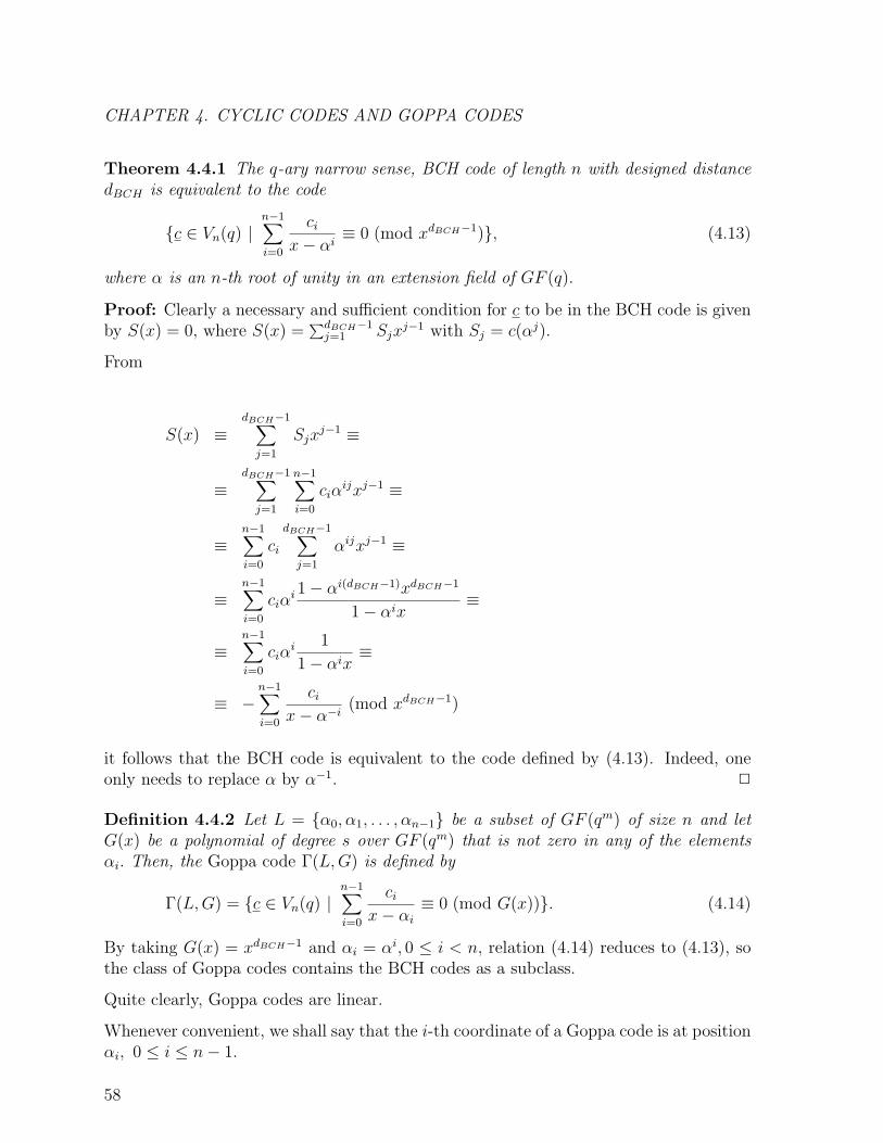
CHAPTER 4. CYCLIC CODES AND GOPPA CODES
Theorem 4.4.1 The q-ary narrow sense, BCH code of length n with designed distancedBCH is equivalent to the code
{c ∈ Vn(q) |n−1∑i=0
cix− αi
≡ 0 (mod xdBCH−1)}, (4.13)
where α is an n-th root of unity in an extension field of GF (q).
Proof: Clearly a necessary and sufficient condition for c to be in the BCH code is givenby S(x) = 0, where S(x) =
∑dBCH−1j=1 Sjx
j−1 with Sj = c(αj).
From
S(x) ≡dBCH−1∑
j=1
Sjxj−1 ≡
≡dBCH−1∑
j=1
n−1∑i=0
ciαijxj−1 ≡
≡n−1∑i=0
ci
dBCH−1∑j=1
αijxj−1 ≡
≡n−1∑i=0
ciαi 1− αi(dBCH−1)xdBCH−1
1− αix≡
≡n−1∑i=0
ciαi 1
1− αix≡
≡ −n−1∑i=0
cix− α−i
(mod xdBCH−1)
it follows that the BCH code is equivalent to the code defined by (4.13). Indeed, oneonly needs to replace α by α−1. 2
Definition 4.4.2 Let L = {α0, α1, . . . , αn−1} be a subset of GF (qm) of size n and letG(x) be a polynomial of degree s over GF (qm) that is not zero in any of the elementsαi. Then, the Goppa code Γ(L,G) is defined by
Γ(L,G) = {c ∈ Vn(q) |n−1∑i=0
cix− αi
≡ 0 (mod G(x))}. (4.14)
By taking G(x) = xdBCH−1 and αi = αi, 0 ≤ i < n, relation (4.14) reduces to (4.13), sothe class of Goppa codes contains the BCH codes as a subclass.
Quite clearly, Goppa codes are linear.
Whenever convenient, we shall say that the i-th coordinate of a Goppa code is at positionαi, 0 ≤ i ≤ n− 1.
58

4.4. GOPPA CODES
Theorem 4.4.3 The Goppa code Γ(L,G) of length n with G(x) of degree s has parame-ters [n,≥ n−ms,≥ s+ 1].
Proof:
i) We shall first show that Γ(L,G) has minimum distance at least s+ 1.
Let c be a codeword of weight w, w > 0 and let the non-zero coordinates of c be atpositions {αi1 , αi2 , . . . , αiw}.
Write the summation in (4.14) as one fraction. Then, because the denominator has nofactor in common with G(x), condition (4.14) is equivalent to stating that the numeratorin (4.14) is divisible by G(x), i.e.
G(x) dividesw(c)∑l=1
cil∏
1≤j≤w,j 6=l
(x− αij).
However this numerator has degree at most w − 1. It follows that w − 1 ≥ s.
ii) To prove the bound on the dimension of Γ(L,G), we write each 1/(x− αi), 0 ≤ i ≤n− 1, as a polynomial Gi(x) =
∑s−1j=0Gijx
j modulo G(x).
Condition (4.14) can now be written as
n−1∑i=0
ciGi(x) ≡ 0 (mod G(x))
or, alternatively, by considering the coefficients of xj, 0 ≤ j ≤ s− 1,
n−1∑i=0
ciGij = 0 for 0 ≤ j ≤ s− 1.
This means that Γ(L,G) can be defined by s linear equations over GF (qm) and thus by≤ ms linear equations over GF (q). Hence, Γ(L,G) has dimension at least n−ms.
2
Example 4.4.4 (to be continued) Let α be the primitive element in GF (24) satisfyingα4 + α3 + 1 = 0. Consider the binary Goppa code Γ(L,G) of length 12 with G(x) =(x+ α)(x+ α14) = x2 + α8x+ 1 and L = {αi | 2 ≤ i ≤ 13}.
The inverses Gi(x) =∑s−1
j=0Gijxj, 2 ≤ i ≤ 13, of (x− αi) modulo G(x) are given by the
columns (Gi0, Gi1)T in the following parity check matrix of Γ(L,G):
H =
(α9 α α8 α13 α7 α5 0 α9 α α6 α5 α6
α14 α3 α α4 α7 α1 α14 α4 α14 α9 α9 α3
).
To check the correctness of the first column of H, i.e. that1
x− α2≡ α9 + α14x
(mod x2 + α8x+ 1), note that
(x− α2)(α9 + α14x) ≡ α11 + α7x+ α14x2 ≡
59
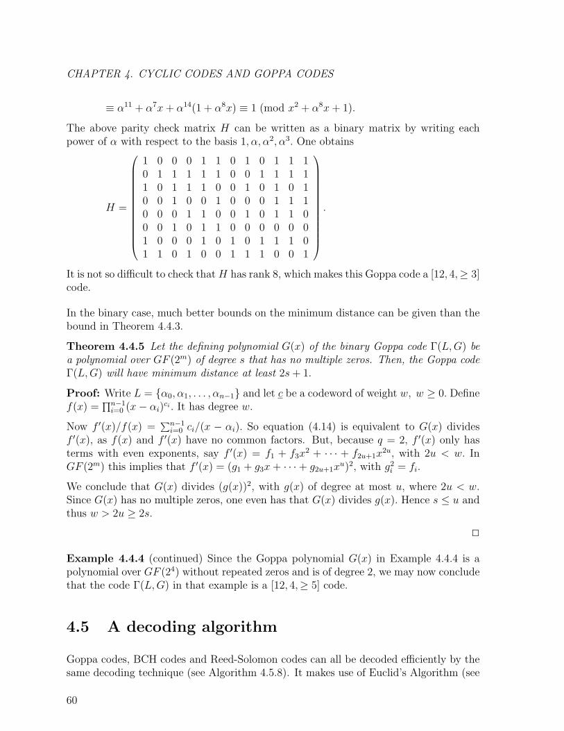
CHAPTER 4. CYCLIC CODES AND GOPPA CODES
≡ α11 + α7x+ α14(1 + α8x) ≡ 1 (mod x2 + α8x+ 1).
The above parity check matrix H can be written as a binary matrix by writing eachpower of α with respect to the basis 1, α, α2, α3. One obtains
H =
1 0 0 0 1 1 0 1 0 1 1 10 1 1 1 1 1 0 0 1 1 1 11 0 1 1 1 0 0 1 0 1 0 10 0 1 0 0 1 0 0 0 1 1 10 0 0 1 1 0 0 1 0 1 1 00 0 1 0 1 1 0 0 0 0 0 01 0 0 0 1 0 1 0 1 1 1 01 1 0 1 0 0 1 1 1 0 0 1
.
It is not so difficult to check thatH has rank 8, which makes this Goppa code a [12, 4,≥ 3]code.
In the binary case, much better bounds on the minimum distance can be given than thebound in Theorem 4.4.3.
Theorem 4.4.5 Let the defining polynomial G(x) of the binary Goppa code Γ(L,G) bea polynomial over GF (2m) of degree s that has no multiple zeros. Then, the Goppa codeΓ(L,G) will have minimum distance at least 2s+ 1.
Proof: Write L = {α0, α1, . . . , αn−1} and let c be a codeword of weight w, w ≥ 0. Definef(x) =
∏n−1i=0 (x− αi)
ci . It has degree w.
Now f ′(x)/f(x) =∑n−1
i=0 ci/(x − αi). So equation (4.14) is equivalent to G(x) dividesf ′(x), as f(x) and f ′(x) have no common factors. But, because q = 2, f ′(x) only hasterms with even exponents, say f ′(x) = f1 + f3x
2 + · · · + f2u+1x2u, with 2u < w. In
GF (2m) this implies that f ′(x) = (g1 + g3x+ · · ·+ g2u+1xu)2, with g2
i = fi.
We conclude that G(x) divides (g(x))2, with g(x) of degree at most u, where 2u < w.Since G(x) has no multiple zeros, one even has that G(x) divides g(x). Hence s ≤ u andthus w > 2u ≥ 2s.
2
Example 4.4.4 (continued) Since the Goppa polynomial G(x) in Example 4.4.4 is apolynomial over GF (24) without repeated zeros and is of degree 2, we may now concludethat the code Γ(L,G) in that example is a [12, 4,≥ 5] code.
4.5 A decoding algorithm
Goppa codes, BCH codes and Reed-Solomon codes can all be decoded efficiently by thesame decoding technique (see Algorithm 4.5.8). It makes use of Euclid’s Algorithm (see
60
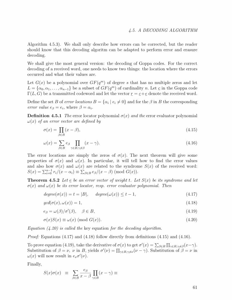
4.5. A DECODING ALGORITHM
Algorithm 4.5.3). We shall only describe how errors can be corrected, but the readershould know that this decoding algoritm can be adapted to perform error and erasuredecoding.
We shall give the most general version: the decoding of Goppa codes. For the correctdecoding of a received word, one needs to know two things: the location where the errorsoccurred and what their values are.
Let G(x) be a polynomial over GF (qm) of degree s that has no multiple zeros and letL = {α0, α1, . . . , αn−1} be a subset of GF (qm) of cardinality n. Let c in the Goppa codeΓ(L,G) be a transmitted codeword and let the vector r = c+e denote the received word.
Define the set B of error locations B = {αi | ei 6= 0} and for the β in B the correspondingerror value eβ = ei, where β = αi.
Definition 4.5.1 The error locator polynomial σ(x) and the error evaluator polynomialω(x) of an error vector are defined by
σ(x) =∏β∈B
(x− β), (4.15)
ω(x) =∑β∈B
eβ
∏γ∈B,γ 6=β
(x− γ). (4.16)
The error locations are simply the zeros of σ(x). The next theorem will give someproperties of σ(x) and ω(x). In particular, it will tell how to find the error valuesand also how σ(x) and ω(x) are related to the syndrome S(x) of the received word:S(x) =
∑n−1i=0 ri/(x− αi) ≡
∑β∈B eβ/(x− β) (mod G(x)).
Theorem 4.5.2 Let e be an error vector of weight t. Let S(x) be its syndrome and letσ(x) and ω(x) be its error locator, resp. error evaluator polynomial. Then
degree(σ(x)) = t = |B|, degree(ω(x)) ≤ t− 1, (4.17)
gcd(σ(x), ω(x)) = 1, (4.18)
eβ = ω(β)/σ′(β), β ∈ B, (4.19)
σ(x)S(x) ≡ ω(x) (mod G(x)). (4.20)
Equation (4.20) is called the key equation for the decoding algorithm.
Proof: Equations (4.17) and (4.18) follow directly from definitions (4.15) and (4.16).
To prove equation (4.19), take the derivative of σ(x) to get σ′(x) =∑
β∈B
∏γ∈B,γ 6=β(x−γ).
Substitution of β = ν, ν in B, yields σ′(ν) =∏
γ∈B,γ 6=ν(ν − γ). Substitution of β = ν inω(x) will now result in eνσ
′(ν).
Finally,
S(x)σ(x) ≡∑β∈B
eβ
x− β∏γ∈B
(x− γ) ≡
61

CHAPTER 4. CYCLIC CODES AND GOPPA CODES
≡∑β∈B
eβ
∏γ∈B,γ 6=β
(x− γ) ≡
≡ ω(x) (mod G(x)). (4.21)
2
Determining σ(x) and ω(x) from (4.21) amounts to applying (the well-known) Euclid’sAlgorithm for polynomials to G(x) and S(x).
Algorithm 4.5.3 (Euclid’s Algorithm) Let a(x) and b(x) be two q-ary polynomials,where degree(a(x)) ≥ degree(b(x)).
Define the sequences of polynomials si(x), ui(x), vi(x) and qi(x), where the degrees ofsi(x) are strictly decreasing, recursively as follows.
s0(x) = a(x), s1(x) = b(x),u0(x) = 1, u1(x) = 0,v0(x) = 0, v1(x) = 1,i = 1.
While si(x) 6= 0 do begin
i := i+ 1Define qi(x) and si(x) by the divisionsi−2(x) = qi(x)si−1(x) + si(x)with degree(si(x)) < degree(si−1(x)).Define ui(x) and vi(x) byui−2(x) = qi(x)ui−1(x) + ui(x),vi−2(x) = qi(x)vi−1(x) + vi(x).end
n=i.
Then
gcd(a(x), b(x)) = sn−1(x) = un−1(x)a(x) + vn−1(x)b(x). (4.22)
Before we can derive the property of the above algorithm that will be essential for thedecoding algorithm, we need three lemmas. Some readers may want to skip these lemmaswith their proofs and move directly to Theorem 4.5.7.
Lemma 4.5.4 The sequences of polynomials defined in Algorithm 4.5.3 satisfy the fol-lowing equations:
62
4.5. A DECODING ALGORITHM
(i) (−1)i+1a(x) = vi(x)si−1(x)− vi−1(x)si(x), 1 ≤ i ≤ n− 1,(ii) (−1)ib(x) = ui(x)si−1(x)− ui−1(x)si(x), 1 ≤ i ≤ n− 1,
(iii) (−1)i = ui(x)vi−1(x)− ui−1(x)vi(x), 1 ≤ i ≤ n− 1,(iv) degree(ui(x))+ degree(si−1(x)) = degree(b(x)), 2 ≤ i ≤ n− 1,(v) degree(vi(x))+ degree(si−1(x)) = degree(a(x)), 1 ≤ i ≤ n− 1,
(vi) si(x) = ui(x)a(x) + vi(x)b(x), 0 ≤ i ≤ n.
Proof: Straightforward induction on i. 2
For our purposes, we are not interested in both the ui(x) and the vi(x) sequences, onlythe vi(x) sequence will do.
Lemma 4.5.5 Let k and l be two nonnegative integers satisfying k+l = degree(a(x))−1and l ≥ degree(gcd(a(x), b(x))). Then there exists a unique integer i, 1 ≤ i ≤ n−1, suchthat
degree(vi(x)) ≤ k, (4.23)
degree(si(x)) ≤ l. (4.24)
Proof: Since the degrees of the polynomials si(x) are strictly decreasing, we can definea unique integer i by
degree(si(x)) ≤ l ≤ degree(si−1(x))− 1. (4.25)
From (v) it follows that
degree(vi(x)) ≤ k ≤ degree(vi+1(x))− 1. (4.26)
These two equations not only imply the existence of the integer i in the statement of thelemma, but also its uniqueness. Indeed equation (4.25) shows that no smaller value of ican be taken, while equation (4.26) shows that no larger value of i is permissable.
2
Relation (vi) can be written as vi(x)b(x) ≡ si(x) (mod a(x)), while (v) (and the de-creasing degrees of the si(x) sequence) implies that degree(vi(x)) + degree(si(x)) <degree(a(x)). The next theorem shows that polynomials v(x) and s(x) with these twoproperties are unique up to a common factor.
Lemma 4.5.6 Let s(x) and v(x) be two non-zero polynomials satisfying
v(x)b(x) ≡ s(x) (mod a(x)), (4.27)
degree(v(x))+ degree(s(x)) < degree(a(x)) (4.28)
Then there exists a unique integer i, 1 ≤ i ≤ n, and a polynomial λ(x) such that
v(x) = λ(x)vi(x) (4.29)
s(x) = λ(x)si(x). (4.30)
63
CHAPTER 4. CYCLIC CODES AND GOPPA CODES
Proof: Let l = degree(s(x)) and k = degree(a(x))− degree(s(x)) − 1. By (4.27)gcd(a(x), b(x)) divides s(x), so l ≥ degree(gcd(a(x), b(x))). Let i be the unique in-teger defined in Lemma 4.5.5 for these values of k and l. From (4.25) it followsthat degree(si−1(x)) ≥ l + 1 ≥ degree(si(x)) + 1. Similarly (4.26) implies thatdegree(vi+1(x)) ≥ k + 1 ≥ degree(vi(x)) + 1. We conclude that if there exists an in-teger i satisfying (4.29) and (4.30) it must be unique and equal to the integer defined byLemma 4.5.5.
Equation (4.27) can be written as
s(x) = u(x)a(x) + v(x)b(x) (4.31)
for some u(x). Property (vi) in Lemma 4.5.4 has a similar form:
si(x) = ui(x)a(x) + vi(x)b(x) (4.32)
Eliminating b(x) from these two relations yields
si(x)v(x) ≡ s(x)vi(x) (mod a(x)).
However, both si(x) and s(x) have degree at most l and both v(x) and vi(x) have degreeat most k. Since k + l < degree(a(x)) we conclude that
si(x)v(x) = s(x)vi(x).
Substituting this back in (4.31) and (4.32) results in
ui(x)v(x) = u(x)vi(x).
But ui(x) and vi(x) have gcd 1 by property (iii) in Lemma 4.5.4, so u(x) = λ(x)ui(x)and v(x) = λ(x)vi(x) for some polynomial λ(x). Substituting these again in (4.31) and(4.32) yields s(x) = λ(x)si(x).
2
We are finally able to give the theorem on which the decoding algorithm for the Goppacodes is based.
Theorem 4.5.7 Let σ(x) and ω(x) be the error-locator and error-evaluator polynomialsof an error pattern of weight at most bs/2c, where s is the degree of the polynomial G(x)of the Goppa code Γ(L,G). Let S(x) be the syndrome of the error pattern. Then
σ(x) = λvi(x), (4.33)
ω(x) = λsi(x), (4.34)
where si(x) and vi(x) are obtained from applying Euclid’s Algorithm to a(x) = G(x) andb(x) = S(x) until degree(si(x)) < bs/2c for the first time and where λ is chosen suchthat λvi(x) is monic.
64
4.5. A DECODING ALGORITHM
Proof: The polynomials σ(x) and ω(x) satisfy the conditions of Lemma 4.5.6, so σ(x) =λ(x)vi(x) and ω(x) = λ(x)si(x). From (4.18) we conclude that λ(x) must be a constant.This has to be chosen so as to make σ(x) monic (see (4.15)).
2
Now we can formulate the decoding algorithm for the class of Goppa codes (and itssubclasses of BCH and Reed-Solomon codes).
So, let Γ(L,G) be a q-ary Goppa code of length n with degree(G(x)) = s and L ={α0, α1, . . . , αn−1} in GF (qm). Let r be a received vector, r = c + e, with weight(e) ≤bs/2c and c in Γ(L,G). Then, by Theorem 4.5.7, the following algorithm applied to rwill output c.
Algorithm 4.5.8 (Decoding Goppa codes) Write r = (r0, r1, . . . , rn−1).
1. Compute the syndrome
S(x) ≡n−1∑i=0
ri
x− αi
(mod G(x)).
2. Apply Euclid’s Algorithm to a(x) = G(x) and b(x) = S(x) until degree(si(x)) <bs/2c for the first time. Let ν be the leading coefficient of vi(x). Set σ(x) = vi(x)/νand ω(x) = si(x)/ν.
3. Find the set B = {β in GF (qm) | σ(β) = 0} of error locations.
4. Determine the error values eβ = ω(β)/σ′(β) for all β in B.
5. Determine e = (e0, e1, . . . , en−1) from ei = eβ if β is in B and β = αi and ei = 0otherwise.
6. Set c = r − e.
Remark 1: In Step 3 in the above algorithm one simply has to try the various αi in Luntil degree(σ(x)) zeros have been found.
Remark 2: The division by ν in Step 2 is not necessary. Indeed, the zeros of σ(x) arenot changed by a scalar multiplication and for the computation of the error values (inStep 4) both numerator and denominator contain the same factor v.
Remark 3: For the decoding of BCH and RS codes over an extension field of GF (2)one can compute the syndrome directly from Sj = r(αj), 1 ≤ j ≤ dBCH − 1. The errorlocations are now however given by the reciprocals of the elements in B. The reason forthis lies in the equivalence of the BCH code and the Goppa code under the mappingα→ α−1 (see the proof of Theorem 4.4.1).
65

CHAPTER 4. CYCLIC CODES AND GOPPA CODES
Let Γ(L,G) be a binary Goppa codes defined by an irreducible Goppa polynomialG(x) of degree s over GF (2m). Then Γ(L,G) is s error-correcting by Theorem 4.4.5.However, Algorithm 4.5.8 will only decode up to bs/2c errors, because the Euclid-ean Algorithm can not be applied directly. Note that in this case (4.16) reduces toω(x) =
∑β∈B
∏γ∈B,γ 6=β(x− γ) = σ′(x). So the key equation (4.20) can now be rewritten
as
σ(x)S(x) ≡ σ′(x) (mod G(x)). (4.35)
By splitting off the squares and the non-squares is σ(x) one can write
σ(x) = α2(x) + xβ2(x) (4.36)
with
degree(α(x)) ≤ s/2 and degree(β(x)) ≤ (s− 1)/2. (4.37)
Since GF (2m) has characteristic 2, it follows that
σ′(x) = β2(x). (4.38)
Because G(x) is irreducible, one can use Euclid’s Algorithm to find the multiplicativeinverse T (x) of S(x) modulo G(x). So T (x) is determined by S(x)T (x) ≡ 1 (mod G(x)).Substituting (4.36) and (4.38) in (4.35) yields
(T (x) + x) β2(x) ≡ α2(x) (mod G(x)). (4.39)
If T (x) = x, one has that α(x) = 0 and thus that σ(x) = xβ2(x). Since σ(x) has norepeated zeros, it follows that β(x) = 1 and that σ(x) = x.
In the case that T (x) 6= x, more work has to be done to find σ(x). First we determinethe uniquely defined polynomial R(x) satisfying R2(x) ≡ T (x) + x (mod G(x)). Indeed,this can be done since squaring polynomials modulo G(x) is a linear mapping, becausethe characteristic of GF (2m) is 2. The inverse of this linear mapping applied to T (x)+xyields R(x) (store this inverse mapping when decoding more words).
After substitution of T (x) + x ≡ R2(x) (mod G(x)) in (4.39), one obtains R2(x)β2(x) ≡α2(x) (mod G(x)) and thus that
R(x)β(x) ≡ α(x) (mod G(x)). (4.40)
It follows that in exactly the same way as in Algorithm 4.5.8 (i.e. by means of Theorem4.5.7) Euclid’s Algorithm can be applied to G(x) and R(x) to determine the polynomialsα(x) and β(x), satisfying (4.37) and (4.40).
Putting σ(x) = α2(x) + xβ2(x) one is now ready to proceed with Algorithm 4.5.8 (onlySteps 3, 5 and 6 are needed, because eβ = 1 for β ∈ B).
It is in the above way that binary Goppa codes can be decoded.
66
4.6. GEOMETRIC GOPPA CODES
4.6 Geometric Goppa codes
The Goppa codes that are discussed in Section 4.4 are now known to belong to a muchlarger class of codes. It was Goppa himself who formulated the generalization. The codesin this larger class are all constructed with the help of algebraic curves and are thereforecalled geometric Goppa codes, algebraic-geometry codes or just AG codes. For a generaltreatment, we refer the reader to the literature. To construct a particular class of codes,we use:
Definition 4.6.1 Let q be a power of a prime and let s and t be two positive integerssuch that gcd(s, q) = 1 and gcd(s, t) = 1. Let f ∈ GF (q)[x] be a q-ary polynomial ofdegree t with no multiple zeros. Let the set P be defined by
P = {(x, y) | ys = f(x), x ∈ GF (q), y ∈ GF (q)}. (4.41)
The set P with its defining equation ys = f(x) is called an algebraic curve, its elementsare called points. Let n denote the cardinality of P and write P = {P1, P2, . . . , Pn}. Fornon-negative m, we define a vector space L(m) of functions by the following linear spanover GF (q)
L(m) = 〈xiyj | is+ jt ≤ m, 0 ≤ i, 0 ≤ j < s〉. (4.42)
The AG-code C(P ,m) is defined as the following set of q-ary vectors:
C(P ,m) = {(u(P1), u(P2), . . . , u(Pn)) | u ∈ L(m)}. (4.43)
Notice that the choice of the parameters s and t and of the function f is suppressed inthe notation C(P ,m).
The first question that arises is: what are the parameters of AG-codes? It is clear thatthe length of an AG-code is given by the number of points in the set P , i.e. by n. Thedimension of an AG-code is related to the dimension of L(m) and is treated in Corollary4.6.5. The restriction j < s in (4.42) can be made, because terms xiyj with j ≥ s canbe reduced by means of the relation ys = f(x). We shall give methods to estimate theminimum distance in Lemma 4.6.6. First, we shall discuss some examples.
Example 4.6.2 The first non-trivial choice for the numbers s and t in Definition 4.6.1is to take s = t = 1. With f(x) = x, the set P consists of the q points (x, x), x ∈ GF (q).The corresponding curve is called an affine line. In the definition of L(m) we now havej = 0 and L(m) is spanned by the monomials xi, 0 ≤ i ≤ m, i.e. L(m) is the space ofpolynomials in x of degree at most m. Clearly, any polynomial in L(m) has at most mzeros.
For 0 ≤ m ≤ q − 1 this code C(P ,m) has dimension k = m + 1 and any non-zerocodeword has at most m coordinates equal to 0. Thus the parameters of this AG-codeare [q,m+1, q−m]. In particular the code meets the Singleton bound (see also Problem4.7.1). Note that for m = q − 1 the code has parameters [q, q, 1] and we will clearly getno larger codes for m > q − 1.
67
CHAPTER 4. CYCLIC CODES AND GOPPA CODES
Example 4.6.3 Consider the finite field GF (4) = GF (2)[x]/(f(x)) with f(x) = x2 +x + 1 and let α be a zero of f(x). Thus GF (4) = {0, 1, α, α2}. Also, let s = 3, t = 2,where t is the degree of f . What are the points in P (see (4.41)), i.e. what (x, y) satisfyy3 = x2 + x+ 1? Obviously we have the point (α, 0) and also (α2, 0) is a point. If y 6= 0then y3 = 1 and only x = 0 or x = 1 do satisfy y3 = f(x). The complete set of pointsbecomes
P = {(α, 0), (α2, 0), (0, 1), (1, 1), (0, α), (1, α), (0, α2), (1, α2)}
The vectorspaces L(m), for the first few values of m are given by:
L(0) = 〈1〉,L(1) = 〈1〉,L(2) = 〈1, y〉,L(3) = 〈1, y, x〉,L(4) = 〈1, y, x, y2〉,L(5) = 〈1, y, x, y2, xy〉,L(6) = 〈1, y, x, y2, xy, x2〉,L(7) = 〈1, y, x, y2, xy, x2, xy2〉.
The pattern is by no means as simple as for the affine line in Example 4.6.2. The equationy3 = x2 + x + 1 corresponds to a so-called elliptic curve. For m ≥ 1, the dimension ofL(m) increases by 1 when m increases by 1 (this is indeed true for larger values of mas follows from Corollary 4.6.5 below). Thus, for 1 ≤ m ≤ 7, the code C(P ,m) hasdimension k = m. The dimension is one lower than in Example 4.6.2, because this timewe have no monomial xiyj with is+ jt = 3i+ 2j = 1.
For the minimum distance, note that the function y ∈ L(2) has two zeros, the points:(α, 0) and (α2, 0). The function x ∈ L(3) has three zeros, the points: (0, 1), (0, α) and(0, α2). In general the number of zeros of a function f ∈ L(m) can be shown to be notlarger than m (see Lemma 4.6.6). We conclude that the code C(P ,m) in this examplehas parameters [8,m, d ≥ 8−m], for 1 ≤ m ≤ 7.
To obtain the dimension of L(m) in general and to clarify the restriction j < s inDefinition 4.6.1, we need the following lemma.
Lemma 4.6.4 Let s, t be positive integers with gcd(s, t) = 1 and let r be any integer.Precisely one of the following two equations has a non-negative integer solution (i, j):
i′ s+ j′ t = st− s− t− r (4.44)
i′′ s+ j′′ t = r (4.45)
68
4.6. GEOMETRIC GOPPA CODES
Proof: Both equations have integer solutions, since gcd(s, t) = 1. Let (i′, j′) and (i′′, j′′)be the unique solutions with 0 ≤ j′, j′′ < s (any solution can be uniquely transformed in asolution satisfying this restriction by adding a proper multiple of the equation ts−st = 0to it). In particular 0 ≤ j′ + j′′ ≤ 2s − 2. Addition of the Equations (4.44) and (4.45)yields
(i′ + i′′)s+ (j′ + j′′)t = st− s− t.
It also follows that s divides (j′ + j′′ + 1)t, hence s divides (j′ + j′′ + 1) and by theinequality on j′ + j′′ above we must have j′ + j′′ +1 = s. Thus i′ + i′′ = −1 and preciselyone of i′ and i′′ is negative. The claim now follows.
2
Corollary 4.6.5 Let g = (s− 1)(t− 1)/2. Then, for m ≥ 2g − 1,
dimension of L(m) = m+ 1− g (4.46)
Proof: Equation (4.45) has no non-negative solutions for r < 0 and, by Lemma 4.6.4,Equation (4.44) will then have a non-negative solution. Thus we can find non-negativesolutions to is + jt = m (see (4.42)) for m > st − s − t = 2g − 1 and the dimension ofL(m) will increase as a function of m for m ≥ 2g. This increase is always by 1, becausethe relation is+ jt = m can not have two solutions with 0 ≤ j < s.
It remains to prove that the dimension of L(2g − 1) is equal to g. But by Lemma 4.6.4,for every 0 ≤ r ≤ g−1, precisely one of Equations (4.44) and (4.45) has a solution (notethat substitution of the values 0 ≤ r ≤ g − 1 in (4.44) and (4.45) covers exactly thewhole range of right hand sides in between 0 and 2g− 1). The g solutions correspond tothe g monomials xiyj that form a basis for L(2g − 1).
2
Lemma 4.6.6 Any non-zero function u(x, y) in L(m) has at most m zeros in P .
Proof: From Definition 4.6.1 we recall that P is s subset of GF (q) × GF (q) and thatthe points in P satisfy ys = f(x) with f(x) of degree t and gcd(s, q) = gcd(s, t) = 1.It follows that an extension field of GF (q) exists, say GF (ql), that contains a primitives-th root of unity ζ. We shall show that even among the points in P ′ = {(x, y) | ys =f(x), x ∈ GF (ql), y ∈ GF (ql)} the function u(x, y) will have at most m zeros.
The points of P ′ can be divided in classes P ′x, each class containing the points with afixed x-coordinate. If x is a zero of f(x), the class P ′x contains one element: (x, 0). Forx with f(x) 6= 0, the class P ′x is equal to {(x, y), (x, ζy), . . . , (x, ζs−1y)} and containss elements. Now, consider the classes in which the zeros of u(x, y) are contained. Weclearly find the same classes if we consider the zeros of the function:
u∗(x, y) = u(x, y) · u(x, ζy) · · ·u(x, ζs−1y). (4.47)
69
CHAPTER 4. CYCLIC CODES AND GOPPA CODES
By (4.42) one can write u(x, y) as
u(x, y) =∑
0≤i,0≤j<s,is+jt≤m
ui,jxiyj, ui,j ∈ GF (q).
If in the evaluation in (4.47) of the product a term
ui0,j0xi0yj0 · ui1,j1x
i1(ζy)j1 · · ·uis−1,js−1xis−1(ζs−1y)js−1 ,
with i0 + i1 + . . .+ is−1 = i and j0 + j1 + . . .+ js−1 = j, occurs then so does the term
uis−1,js−1xis−1yjs−1 · ui0,j0x
i0(ζy)j0 · · ·uis−2,js−2xis−2(ζs−1y)js−2 ,
which is just the previous term multiplied by ζj0+j1+...+js−1 = ζj. For the same reason, thisterm also occurs multiplied by each of ζ2j, . . . , ζ(s−1)j. It follows from 1+ζj+. . .+ζj(s−1) =0, 1 ≤ j ≤ s− 1, that these s terms cancel, unless j is a multiple of s, say j = sj′.
We conclude that u∗(x, y) only consists of monomials of the form xi′yj′s. With thesubstitution ys = f(x), we can eliminate y from the product (4.47) and write
u∗(x, y) = U(x, ys) = U(x, f(x)) = V (x).
After substitution of ys = f(x) in U , the monomial xi(ys)j′ is of degree i+ tj′ in x. Thisdegree satisfies
s(i+ tj′) = si+ tj
= (si0 + tj0) + (si1 + tj1) + . . .+ (sis−1 + tjs−1)
≤ m+m+ . . .+m = sm.
Thus V (x) is a polynomial in x of degree at most m and the zeros of u∗(x, y) in P ′ canbe grouped into at most m classes. A class P ′x with s elements contributes at most onezero of u(x, y) (and at most one zero to each of the other u(x, ζky), 1 ≤ k ≤ s − 1). Aclass P ′x of the form {(x, 0)} trivially contains at most one zero of u(x, y). So, each ofthe at most m classes containing zeros of u(x, y) contributes at most one such zero in P .
2
We can now give the parameters of AG-codes (see Definition 4.6.1).
Theorem 4.6.7 Let C(P ,m) be an AG − code as defined in Definition 4.6.1. Let gbe given by Corollary 4.6.5 and let 2g − 1 ≤ m < n. Then, C(P ,m) has parameters[n,m+ 1− g, n−m].
Proof: The length of C(P ,m) is simply equal to the cardinality of the set P . Sincem < n, Lemma 4.6.6 implies that the space L(m) contains no non-zero function that iszero at all points in P . In particular the space L(m) and the code C(P ,m) are isomorphicas vector spaces and they have the same dimension. With m ≥ 2g−1, the dimension now
70
4.6. GEOMETRIC GOPPA CODES
follows from Corollary 4.6.5. The minimum distance follows immediately from Lemma4.6.6.
2
Comparison of the parameters of an AG-code with the Singleton bound (see Equation(2.17)) shows that for small values of g the AG-codes are almost optimal. Larger valuesof g will still yield good codes, provided that the curve P has many points.
Let C∗(P ,m) denote the dual code of C(P ,m). It is also called an AG-code. It can bedescribed using the same set of points P , but using a different vector space of functions.For our purposes it is enough to realize that for the description of C∗(P ,m) (by meansof a generator matrix and a parity check matrix) it is enough to have a description ofC(P ,m). We shall now derive a decoding procedure for the dual code C∗(P ,m). FromTheorem 4.6.7 we already know that C∗(P ,m) is a q-ary code of length n and dimensionn−(m+1−g). Its minimum minimum distance will follow from the decoding procedure.
We need several lemmas. Let r = c + e be a received word, with c the transmittedcodeword in C∗(P ,m) and e the error vector. Let the points Pk, 1 ≤ k ≤ n, in P havecoordinates (xk, yk). It follows that
∑nk=1 ckx
iky
jk = 0 for the pairs (i, j) with is + jt ≤
m, 0 ≤ i, 0 ≤ j < s.
Definition 4.6.8 Define the degree of a monomial φ(x, y) = xiyj by is+ jt and assumethat the monomials φ(x, y) are put in order of increasing (see Corollary 4.6.5) degree.Thus, if the space L(m) is of dimension M , we may write
L(m) = 〈φ1 = 1, φ2, . . . , φM〉.
For any pair of integers (i, j), we define the 1st order syndrome of the vector e as
Si,j =n∑
k=1
ekxiky
jk (4.48)
and call is+ jt the degree of Si,j.
For any pair of positive integers (u, v) with φu(x, y) = xi1yj1 and φv(x, y) = xi2yj2 , wedefine the 2nd order syndrome
Tu,v =n∑
k=1
ekφu(Pk)φv(Pk) (4.49)
and call degree(φuφv) = (i1 + i2)s+ (j1 + j2)t the degree of Tu,v.
It follows from this definition that for all u, v ≥ 1
Tu,v = Si1+i2,j1+j2 . (4.50)
Using Equation (4.50) one can find the Si,j from the Tu,v and vice versa (take v = 1 togo from Tu,v to Si,j). Note that by (4.41) each Si,j with j ≥ s can be expressed in termsof the Si,j’s with j < s.
71
CHAPTER 4. CYCLIC CODES AND GOPPA CODES
If a 1st order syndrome Si,j of degree m exists it is unique if we choose it with 0 ≤i, 0 ≤ j < s. There can be several 2nd order syndromes of a given degree. Indeed, Tv,u
and Tu,v are obviously equal to each other and there may be other pairs (u′, v′) withdegree(Tu′,v′) = degree(Tu,v). This fact will be exploited later.
Note that the 1st order syndrome Si,j of the error vector e and of the received vectorr is the same for the pairs (i, j) with xiyj ∈ L(m). So, from a received vector one candirectly compute the following 1st and 2nd order syndromes
Si,j, for is+ jt ≤ m, 0 ≤ i, 0 ≤ j < s,
Tu,v, for φu · φv ∈ L(m).
These are the syndromes of degree at most m.
Lemma 4.6.9 The error vector (e1, e2, . . . , en) is uniquely determined by the 1st ordersyndromes Si,j, for i, j ∈ {0, 1, . . . , q − 2}. It can be computed with an inverse Fouriertransform.
Proof: Let 1 ≤ l ≤ n and let the coordinates (xl, yl) of Pl be non-zero, say xl = αg, yl =αh. Since
∑q−2i=0 a
i = 0 for a ∈ GF (q) \ {0, 1}, one has
q−2∑i=0
q−2∑j=0
Si,j · (αu)i · (αv)j =q−2∑i=0
q−2∑j=0
n∑k=1
ekxiky
jk(α
u)i(αv)j =
=n∑
k=1
ek
q−2∑i=0
(xkαu)i
q−2∑j=0
(ykαv)j
=
{0 if (u, v) 6= (−g,−h),el if (u, v) = (−g,−h).
We leave the case xl = 0 or yl = 0 as an exercise to the reader.
2
It follows from this lemma that it is sufficient for the decoding of C∗(P ,m) to determinethe 1st order syndromes Si,j up to degree (q−2)(s+t). We shall show how the syndromesSi,j with degree is + jt in {m + 1,m + 2, . . . , (q − 2)(s + t)} can be determined one byone.
To obtain Si,j of degree m+ 1 we consider all Tu,v of degree m+ 1, i.e. all Tu,v with
φu · φv ∈ L(m+ 1) \ L(m). (4.51)
To compute these Tu,v’s, the crucial step is to put them in an array.
72
4.6. GEOMETRIC GOPPA CODES
Lemma 4.6.10 Let the matrix T(u,v) be defined as
T(u,v) = (Ti,j) 1≤i≤u,1≤j≤v.
Then matrix T(u,v) has rank at most τ = wH(e).
Proof: Let G(u) and G(v) be generator matrices for codes C(P , u∗) of dimension u andC(P , v∗) of dimension v resp. (so L(u∗) = 〈φ1, φ2, . . . , φu〉, and L(v∗) = 〈φ1, φ2, . . . , φv〉).Let ∆(e) denote the matrix with (e1, e2, . . . , en) on the main diagonal and zeros else-where. We have by (4.49) that
T(u,v) = G(v) ·∆(e) ·G(u)T , (4.52)
and the rank of T(u,v) is obviously at most equal to τ .
2
We denote by T any sufficiently large array that contains each matrix T(u,v) as submatrixin its upper-left corner. An upper bound on the size of T is (q−2)(s+ t)× (q−2)(s+ t).
Although the following lemma is stated for the submatrices of T, it will be clear fromthe proof that it holds for the submatrices of any matrix.
Lemma 4.6.11 Let the positive integers u, v satisfy
rank T(u−1,v−1) = rank T(u−1,v) = rank T(u,v−1). (4.53)
Then, there exists a unique value for the entry Tu,v, such that
rank T(u,v) = rank T(u−1,v−1). (4.54)
Proof: It follows from rank T(u−1,v−1) = rank T(u,v−1) that coefficients αa, 1 ≤ a ≤ u−1,exist such that Tu,b =
∑u−1a=1 αaTa,b, 1 ≤ b ≤ v − 1. If Tu,v 6=
∑u−1a=1 αaTa,v, the rank of
T(u,v) will obviously be one more than the rank of T(u−1,v−1). From this contradictionwith (4.54) the unique choice of Tu,v follows.
On the other hand, taking Tu,v =∑u−1
a=1 αaTa,v, we obtain rank T(u,v) = rank T(u−1,v) =rank T(u−1,v−1).
2
Definition 4.6.12 A pair (u, v) that satisfies (4.53), but fails (4.54) is called a discrep-ancy of T.
A pair (u, v) with Tu,v satisfying (4.51) for which condition (4.53) holds is called acandidate. A candidate is called correct if also condition (4.54) is fulfilled. Otherwise itis called an incorrect candidate.
It is easy to show (by elementary row and column operations) that no row or column ofa matrix can contain two discrepancies. Another way to look at the discrepancies of T(or any other matrix) is given by the following lemma.
73
CHAPTER 4. CYCLIC CODES AND GOPPA CODES
Lemma 4.6.13 The rank of T(u,v) equals the number of discrepancies among (i, j) with1 ≤ i ≤ u, 1 ≤ j ≤ v.
A pair (u, v) satisfies (4.53) if and only if there are no discrepancies among (i, v), i < uand (u, j), j < v.
Proof: Consider T(u,v) (start this procedure with the empty submatrix T(0,0)). Aslong as rank T(u,v+1) = rank T(u,v), increase v by one (this argument also holds forrows). If rank T(u,v+1) = rank T(u,v) + 1, there will be exactly one discrepancy amongthe positions (i, v + 1), 1 ≤ i ≤ u. This is position (1, v + 1), if rank T(1,v) = 0 andrank T(1,v+1) = 1, and position (i, v + 1) where i is the smallest/unique value withrank T(i,v+1) = rank T(i,v) + 1. Note that i is less than or equal to u.
The second statement now follows from the first.
2
With the available information on the 2nd order syndromes it is possible to determine ifthe pair (u, v) is a candidate, but not if it is a correct or an incorrect candidate. On theassumption that a candidate is correct its value can be uniquely determined by Lemma4.6.11.
In the decoding algorithm we shall consider all candidates (u, v) and simply assumethat they are correct (which may not always be the case). Then we determine thesyndromes Tu,v for these candidates by means of Lemma 4.6.11 and for each we computethe corresponding Si,j of degree m (by (4.50)). Assuming that the number of errors τ islimited, the number of discrepancies will also be limited by Lemmas 4.6.10 and 4.6.13.Assuming that we can show that the number of correct candidates exceeds the number ofincorrect candidates, we can recongnize the correct value of Si,j among all the computedSi,j’s with an easy majority vote.
Lemma 4.6.14 Let m ≥ 4g − 2. The array T contains N := m + 2 − 2g pairs (u, v)satisfying (4.51). No two of these pairs lie in the same row or column.
Proof: Consider a pair (u, v) satisfying (4.51), i.e. φu · φv ∈ L(m + 1) \ L(m). Clearlynot both φu and φv can be in L(2g − 1), since then φu · φv ∈ L(4g − 2) ⊆ L(m).Thus, by Lemma 4.6.5, we find g pairs (u, v) with φu ∈ L(2g − 1) (for each of theseu’s there is a unique v with φu · φv ∈ L(m + 1) \ L(m) because m + 1− degree (φu) ≥m + 1 − (2g − 1) ≥ 2g) and, for the same reason, g pairs with φv ∈ L(2g − 1). Forφu, φv 6∈ L(2g− 1), we must have φu, φv ∈ L(m+ 1− 2g) \L(2g− 1). This gives anotherm + 1 − 2g − (2g − 1) = m + 2 − 4g pairs, yielding a total of m + 2 − 2g pairs (u, v)satisfying (4.51).
The second assertion also follows trivially, because from degree(Tu,v) = degree(Tu′,v′) itfollows that u = u′ if and only if v = v′.
2
74

4.6. GEOMETRIC GOPPA CODES
Lemma 4.6.15 Let D be the number of known discrepancies. Among the N pairs (u, v)satisfying (4.51) are at least N − 2D candidates.
Proof: From the second statement in Lemma 4.6.13 we know that each of the N pairssatisfying (4.51) is a candidate if it has no discrepancy in its row or column. By Lemma4.6.14 no two of these N pairs occur in the same row or column. It follows that each ofthe D discrepancies prevents at most two pairs from being a candidate.
2
Lemma 4.6.16 Among all candidates no more than τ −D discrepancies can occur.
Proof: The total number of discrepancies can not exceed the rank of the array T which isat most τ . Since D discrepancies are already known (at pairs (u, v) with φu ·φv ∈ L(m)),at most τ −D discrepancies can occur at pairs that are candidates.
2
Lemma 4.6.17 Let m ≥ 4g − 2 (as in Lemma 4.6.14) and 2τ < m+ 2− 2g. Then thenumber of correct candidates T will exceed the number of incorrect candidates F .
Proof: This follows from the inequality
T + F ≥ N − 2D = m+ 2− 2g − 2τ + 2τ − 2D
> 2τ − 2D ≥ 2F,
where the first inequality follows from Lemma 4.6.15, the equality from Lemma 4.6.14,the second inequality from the condition on τ, and the last inequality from Lemma 4.6.16.
2
We can now put all the steps of the decoding algorithm of AG-codes together.
Algorithm 4.6.18 (Decoding AG-codes) Let m ≥ 4g − 2 and let r = c + e be areceived word, where c ∈ C∗(P ,m) and e is an error vector of weight τ ≤ b(m+1−2g)/2c.
1. Compute the 1st order syndromes Si,j of r for all is+ jt ≤ m, 0 ≤ i, 0 ≤ j < s bymeans of (4.48).
2. Compute the 2nd order syndromes Tu,v for all (u, v) with φu · φv ∈ L(m) by meansof (4.50).
3. For m′ = m + 1,m + 2, . . . , (q − 2)(s + t) determine the candidates (u, v) andassume that they are all correct. For each candidate (u, v) compute Tu,v by meansof Lemma 4.6.11 and the corresponding Si,j of degree m′ with (4.50). The correctvalue of Si,j is obtained by taking a majority decision over the obtained values. Usethe correct value of Si,j to compute all Tu,v of degree m′ in T.
75
CHAPTER 4. CYCLIC CODES AND GOPPA CODES
4. Compute the error vector e from the 1st order syndromes Si,j, 0 ≤ i, j ≤ q − 2, bymeans of Lemma 4.6.9.
5. Put c = r − e.
Theorem 4.6.19 The code C∗(P ,m), with m ≥ 4g−2, has parameters [n, n−m−1+g,≥m+ 2− 2g].
Proof: Since C∗(P ,m) is the dual code of the [n,m + 1 − g, n −m] code C(P ,m), ithas length n and dimension n −m − 1 + g. The decoding algorithm above shows thatthe minimum distance is at least equal to m+ 2− 2g for m odd. This can however alsobe shown to hold for m even.
2
Note that, just as as C(P ,m), also C∗(P ,m) satisfies the bound k + d ≥ n + 1 − g(compare this with the Singleton bound (Equation 2.17).
For large q we need to compute a large number of Si,j’s before Lemma 4.6.17 can beapplied. To obtain all the required syndromes, Step 3 in Algorithm 4.6.18 needs to berepeated many times. In this situation the following theorem is useful. It combinesthe procedure that we have presented with another procedure, for which we refer to theliterature (see the remarks at the end of the section).
Theorem 4.6.20 For a curve with g ≥ 1, consider the matrix T (τ+g,τ+g). In general,not all entries can be computed with the syndromes of the received vector. We look for alinear relation among the known columns, i.e. for a solution of
T (τ+g,τ+g)a = 0,
where ai = 0 if the i-th column of T (τ+g,τ+g) contains an unknown entry.
If no nonzero solution a exists, it suffices in Step 3 of Algorithm 4.6.18 to compute onlythe candidates (u, v) with 1 ≤ u, v ≤ τ + g. A majority decision among these will yieldthe syndrome of degree m′. If a nonzero solution a does exist, the algorithm can beterminated as follows.
Let f = a1φ1 + a2φ2 + . . . + aτ+gφτ+g. Then f(Pk) = 0, for ek 6= 0. Applying erasuredecoding to the zeros of f yields the error vector as a unique solution.
We omit the full proof, but make some observations. Note that a nonzero solution a canbe obtained as soon as all entries in the τ + 1-th column are known. The entry Tτ+g,τ+1
is thus the syndrome of highest degree that needs to be known. With Corollary 4.6.5 ithas degree at most (τ + g + g − 1) + (τ + 1 + g − 1). For 2τ < m + 2 − 2g the degreeis bounded by 2τ + 3g − 1 ≤ m + g. Thus, indeed not all the required entries can becomputed with the syndromes of the received vector, but it is only necessary to applyStep 3 in Algorithm 4.6.18 with m′ = m+ 1,m+ 2, . . . ,m+ g.
76
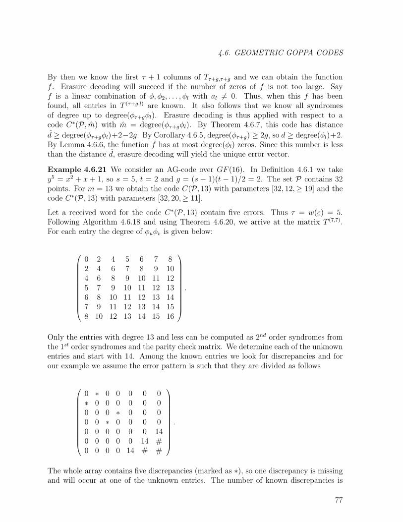
4.6. GEOMETRIC GOPPA CODES
By then we know the first τ + 1 columns of Tτ+g,τ+g and we can obtain the functionf . Erasure decoding will succeed if the number of zeros of f is not too large. Sayf is a linear combination of φ, φ2, . . . , φl with al 6= 0. Thus, when this f has beenfound, all entries in T (τ+g,l) are known. It also follows that we know all syndromesof degree up to degree(φτ+gφl). Erasure decoding is thus applied with respect to acode C∗(P , m) with m = degree(φτ+gφl). By Theorem 4.6.7, this code has distance
d ≥ degree(φτ+gφl)+2−2g. By Corollary 4.6.5, degree(φτ+g) ≥ 2g, so d ≥ degree(φl)+2.By Lemma 4.6.6, the function f has at most degree(φl) zeros. Since this number is lessthan the distance d, erasure decoding will yield the unique error vector.
Example 4.6.21 We consider an AG-code over GF (16). In Definition 4.6.1 we takey5 = x2 + x + 1, so s = 5, t = 2 and g = (s − 1)(t − 1)/2 = 2. The set P contains 32points. For m = 13 we obtain the code C(P , 13) with parameters [32, 12,≥ 19] and thecode C∗(P , 13) with parameters [32, 20,≥ 11].
Let a received word for the code C∗(P , 13) contain five errors. Thus τ = w(e) = 5.Following Algorithm 4.6.18 and using Theorem 4.6.20, we arrive at the matrix T (7,7).For each entry the degree of φuφv is given below:
0 2 4 5 6 7 82 4 6 7 8 9 104 6 8 9 10 11 125 7 9 10 11 12 136 8 10 11 12 13 147 9 11 12 13 14 158 10 12 13 14 15 16
.
Only the entries with degree 13 and less can be computed as 2nd order syndromes fromthe 1st order syndromes and the parity check matrix. We determine each of the unknownentries and start with 14. Among the known entries we look for discrepancies and forour example we assume the error pattern is such that they are divided as follows
0 ∗ 0 0 0 0 0∗ 0 0 0 0 0 00 0 0 ∗ 0 0 00 0 ∗ 0 0 0 00 0 0 0 0 0 140 0 0 0 0 14 #0 0 0 0 14 # #
.
The whole array contains five discrepancies (marked as ∗), so one discrepancy is missingand will occur at one of the unknown entries. The number of known discrepancies is
77
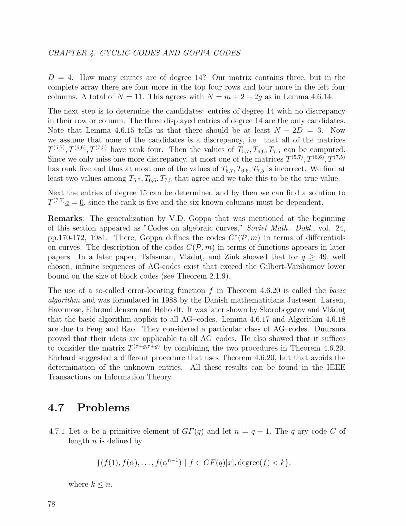
CHAPTER 4. CYCLIC CODES AND GOPPA CODES
D = 4. How many entries are of degree 14? Our matrix contains three, but in thecomplete array there are four more in the top four rows and four more in the left fourcolumns. A total of N = 11. This agrees with N = m+ 2− 2g as in Lemma 4.6.14.
The next step is to determine the candidates: entries of degree 14 with no discrepancyin their row or column. The three displayed entries of degree 14 are the only candidates.Note that Lemma 4.6.15 tells us that there should be at least N − 2D = 3. Nowwe assume that none of the candidates is a discrepancy, i.e. that all of the matricesT (5,7), T (6,6), T (7,5) have rank four. Then the values of T5,7, T6,6, T7,5 can be computed.Since we only miss one more discrepancy, at most one of the matrices T (5,7), T (6,6), T (7,5)
has rank five and thus at most one of the values of T5,7, T6,6, T7,5 is incorrect. We find atleast two values among T5,7, T6,6, T7,5 that agree and we take this to be the true value.
Next the entries of degree 15 can be determined and by then we can find a solution toT (7,7)a = 0, since the rank is five and the six known columns must be dependent.
Remarks: The generalization by V.D. Goppa that was mentioned at the beginningof this section appeared as ”Codes on algebraic curves,” Soviet Math. Dokl., vol. 24,pp.170-172, 1981. There, Goppa defines the codes C∗(P ,m) in terms of differentialson curves. The description of the codes C(P ,m) in terms of functions appears in laterpapers. In a later paper, Tsfasman, Vladut, and Zink showed that for q ≥ 49, wellchosen, infinite sequences of AG-codes exist that exceed the Gilbert-Varshamov lowerbound on the size of block codes (see Theorem 2.1.9).
The use of a so-called error-locating function f in Theorem 4.6.20 is called the basicalgorithm and was formulated in 1988 by the Danish mathematicians Justesen, Larsen,Havemose, Elbrønd Jensen and Høholdt. It was later shown by Skorobogatov and Vladutthat the basic algorithm applies to all AG–codes. Lemma 4.6.17 and Algorithm 4.6.18are due to Feng and Rao. They considered a particular class of AG–codes. Duursmaproved that their ideas are applicable to all AG–codes. He also showed that it sufficesto consider the matrix T (τ+g,τ+g) by combining the two procedures in Theorem 4.6.20.Ehrhard suggested a different procedure that uses Theorem 4.6.20, but that avoids thedetermination of the unknown entries. All these results can be found in the IEEETransactions on Information Theory.
4.7 Problems
4.7.1 Let α be a primitive element of GF (q) and let n = q − 1. The q-ary code C oflength n is defined by
{(f(1), f(α), . . . , f(αn−1) | f ∈ GF (q)[x], degree(f) < k},
where k ≤ n.
78
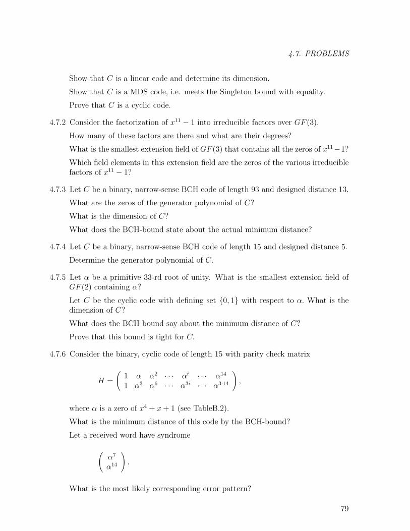
4.7. PROBLEMS
Show that C is a linear code and determine its dimension.
Show that C is a MDS code, i.e. meets the Singleton bound with equality.
Prove that C is a cyclic code.
4.7.2 Consider the factorization of x11 − 1 into irreducible factors over GF (3).
How many of these factors are there and what are their degrees?
What is the smallest extension field of GF (3) that contains all the zeros of x11−1?
Which field elements in this extension field are the zeros of the various irreduciblefactors of x11 − 1?
4.7.3 Let C be a binary, narrow-sense BCH code of length 93 and designed distance 13.
What are the zeros of the generator polynomial of C?
What is the dimension of C?
What does the BCH-bound state about the actual minimum distance?
4.7.4 Let C be a binary, narrow-sense BCH code of length 15 and designed distance 5.
Determine the generator polynomial of C.
4.7.5 Let α be a primitive 33-rd root of unity. What is the smallest extension field ofGF (2) containing α?
Let C be the cyclic code with defining set {0, 1} with respect to α. What is thedimension of C?
What does the BCH bound say about the minimum distance of C?
Prove that this bound is tight for C.
4.7.6 Consider the binary, cyclic code of length 15 with parity check matrix
H =
(1 α α2 · · · αi · · · α14
1 α3 α6 · · · α3i · · · α3·14
),
where α is a zero of x4 + x+ 1 (see TableB.2).
What is the minimum distance of this code by the BCH-bound?
Let a received word have syndrome
(α7
α14
).
What is the most likely corresponding error pattern?
79
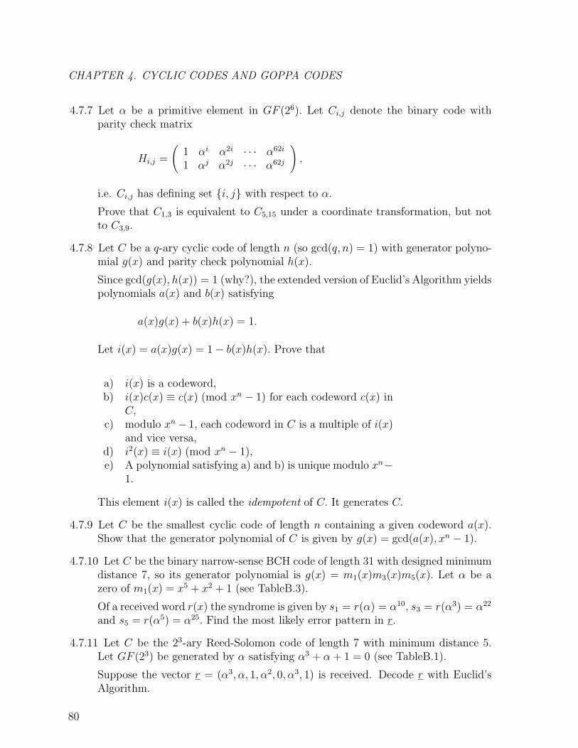
CHAPTER 4. CYCLIC CODES AND GOPPA CODES
4.7.7 Let α be a primitive element in GF (26). Let Ci,j denote the binary code withparity check matrix
Hi,j =
(1 αi α2i · · · α62i
1 αj α2j · · · α62j
),
i.e. Ci,j has defining set {i, j} with respect to α.
Prove that C1,3 is equivalent to C5,15 under a coordinate transformation, but notto C3,9.
4.7.8 Let C be a q-ary cyclic code of length n (so gcd(q, n) = 1) with generator polyno-mial g(x) and parity check polynomial h(x).
Since gcd(g(x), h(x)) = 1 (why?), the extended version of Euclid’s Algorithm yieldspolynomials a(x) and b(x) satisfying
a(x)g(x) + b(x)h(x) = 1.
Let i(x) = a(x)g(x) = 1− b(x)h(x). Prove that
a) i(x) is a codeword,b) i(x)c(x) ≡ c(x) (mod xn − 1) for each codeword c(x) in
C,c) modulo xn− 1, each codeword in C is a multiple of i(x)
and vice versa,d) i2(x) ≡ i(x) (mod xn − 1),e) A polynomial satisfying a) and b) is unique modulo xn−
1.
This element i(x) is called the idempotent of C. It generates C.
4.7.9 Let C be the smallest cyclic code of length n containing a given codeword a(x).Show that the generator polynomial of C is given by g(x) = gcd(a(x), xn − 1).
4.7.10 Let C be the binary narrow-sense BCH code of length 31 with designed minimumdistance 7, so its generator polynomial is g(x) = m1(x)m3(x)m5(x). Let α be azero of m1(x) = x5 + x2 + 1 (see TableB.3).
Of a received word r(x) the syndrome is given by s1 = r(α) = α10, s3 = r(α3) = α22
and s5 = r(α5) = α25. Find the most likely error pattern in r.
4.7.11 Let C be the 23-ary Reed-Solomon code of length 7 with minimum distance 5.Let GF (23) be generated by α satisfying α3 + α+ 1 = 0 (see TableB.1).
Suppose the vector r = (α3, α, 1, α2, 0, α3, 1) is received. Decode r with Euclid’sAlgorithm.
80
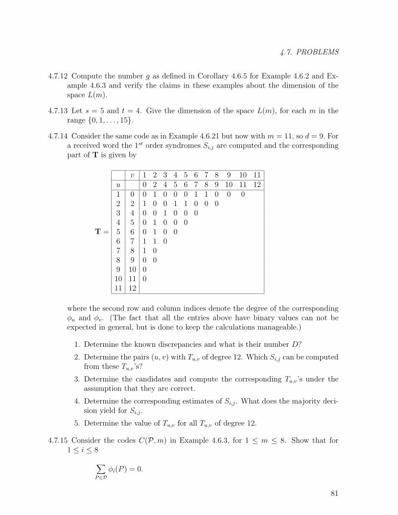
4.7. PROBLEMS
4.7.12 Compute the number g as defined in Corollary 4.6.5 for Example 4.6.2 and Ex-ample 4.6.3 and verify the claims in these examples about the dimension of thespace L(m).
4.7.13 Let s = 5 and t = 4. Give the dimension of the space L(m), for each m in therange {0, 1, . . . , 15}.
4.7.14 Consider the same code as in Example 4.6.21 but now with m = 11, so d = 9. Fora received word the 1st order syndromes Si,j are computed and the correspondingpart of T is given by
T =
v 1 2 3 4 5 6 7 8 9 10 11u 0 2 4 5 6 7 8 9 10 11 121 0 0 1 0 0 0 1 1 0 0 02 2 1 0 0 1 1 0 0 03 4 0 0 1 0 0 04 5 0 1 0 0 05 6 0 1 0 06 7 1 1 07 8 1 08 9 0 09 10 010 11 011 12
where the second row and column indices denote the degree of the correspondingφu and φv. (The fact that all the entries above have binary values can not beexpected in general, but is done to keep the calculations manageable.)
1. Determine the known discrepancies and what is their number D?
2. Determine the pairs (u, v) with Tu,v of degree 12. Which Si,j can be computedfrom these Tu,v’s?
3. Determine the candidates and compute the corresponding Tu,v’s under theassumption that they are correct.
4. Determine the corresponding estimates of Si,j. What does the majority deci-sion yield for Si,j.
5. Determine the value of Tu,v for all Tu,v of degree 12.
4.7.15 Consider the codes C(P ,m) in Example 4.6.3, for 1 ≤ m ≤ 8. Show that for1 ≤ i ≤ 8
∑P∈P
φi(P ) = 0.
81
CHAPTER 4. CYCLIC CODES AND GOPPA CODES
Use this to prove that for 1 ≤ m ≤ 7,
C∗(P ,m) = C(P , 8−m).
82

Chapter 5
Burst correcting codes
5.1 Introduction; two bounds
In many applications, especially those where data are stored on a magnetic medium,errors tend to occur in clusters rather than completely independently of each other.
Definition 5.1.1 In Vn(q) a vector e is called a burst of length b if it has the form
(0, 0, . . . , 0,b︷ ︸︸ ︷
ei, ei+1, . . . , ei+b−1, 0, 0, . . . , 0), (5.1)
where ei 6= 0 and ei+b−1 6= 0.
The segment (ei, ei+1, . . . , ei+b−1) is called the burst pattern. Also, one says that thisburst starts at coordinate i.
Codes that can correct any burst of length up to b are called b-burst-correcting. In thischapter we shall only be interested in linear b-burst-correcting codes.
Lemma 5.1.2 A linear code C is b-burst-correcting if and only if all bursts of length upto b have distinct syndromes.
Proof: Clearly, if distinct bursts have distinct syndromes, one can correct them.
On the other hand, if bursts b1 and b2 of length at most b have the same syndrome,their difference b1 − b2 will be a codeword! The received word b1 can now be written asc1 + b1 with c1 = 0 in C, but also as c2 + b2 with c2 = b1 − b2 also in C. So C is notb-burst-correcting.
2
Lemma 5.1.3 Let C be a linear b-burst-correcting code with parity check matrix H.Then any two disjoint groups of b consecutive columns of H consist of 2b independentvectors.
83
CHAPTER 5. BURST CORRECTING CODES
Proof: If not, there exists a non-trivial dependency of the 2b columns, corresponding tothe two disjoint groups of b consecutive coordinates. This dependency can be representedby two distinct bursts of length b each, say b1 and b2.
The dependency now reads like H(b1 + b2)T = 0T . This implies that the bursts b1 and
−b2 have the same syndrome. This contradicts Lemma 5.1.2.
2
An immediate consequence of Lemma 5.1.3 is the following bound.
Theorem 5.1.4 (Reiger bound) Let C be a q-ary, k-dimensional, b-burst-correctingcode of length n. Then the redundancy r = n− k satisfies
r ≥ 2b, (5.2)
so |C| ≤ qn−2b.
In the sequel we shall often refer to the Reiger bound.
Many of the b-burst-correcting codes that will be constructed further on will be cyclic.It turns out that they are able to correct all cyclic shifts of bursts of length up to b, inparticular those that start near the end and that end somewhere at the beginning of theword, i.e. error patterns of the form:
(
b−(n−i)︷ ︸︸ ︷e0, . . . , eb−(n−i)−1, 0, 0, . . . . . . , 0, 0,
n−i︷ ︸︸ ︷ei, . . . , en−1), (5.3)
where i > n− b, ei 6= 0 and eb−(n−i)−1 6= 0.
Error vectors of the form (5.3) are called cyclic bursts and cyclic codes that can correctall cyclic bursts of length up to b are called cyclic b-burst-correcting.
Again Lemma 5.1.2 can be applied to derive a bound.
Theorem 5.1.5 (Abramson bound) Let C be a q-ary, cyclic b-burst-correcting codeof length n. Then its redundancy r satisfies
n ≤ qr−b+1 − 1
q − 1. (5.4)
Proof: Let us count the number of distinct non-zero cyclic bursts. Each one is definedby its starting coordinate (n possibilities), a non-zero entry there (q−1 choices) followedby b − 1 arbitrarily chosen coordinates. So their number is n(q − 1)qb−1. Now all thesevectors and also the 0-vector should have distinct syndromes. So
qr ≥ 1 + n(q − 1)qb−1.
Dividing this by qb−1 yields
qr−b+1 ≥ 1
qb−1+ n(q − 1)
84
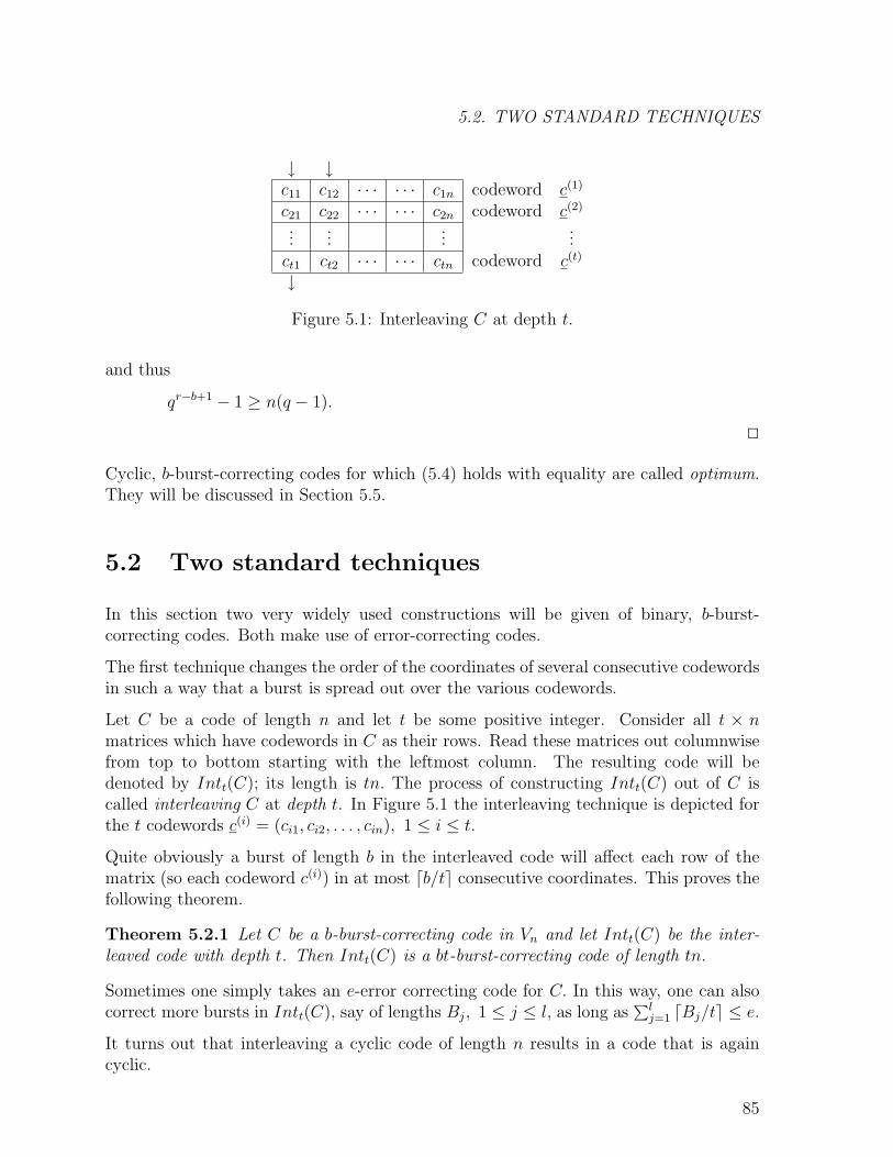
5.2. TWO STANDARD TECHNIQUES
↓ ↓c11 c12 · · · · · · c1n codeword c(1)
c21 c22 · · · · · · c2n codeword c(2)
......
......
ct1 ct2 · · · · · · ctn codeword c(t)
↓
Figure 5.1: Interleaving C at depth t.
and thus
qr−b+1 − 1 ≥ n(q − 1).
2
Cyclic, b-burst-correcting codes for which (5.4) holds with equality are called optimum.They will be discussed in Section 5.5.
5.2 Two standard techniques
In this section two very widely used constructions will be given of binary, b-burst-correcting codes. Both make use of error-correcting codes.
The first technique changes the order of the coordinates of several consecutive codewordsin such a way that a burst is spread out over the various codewords.
Let C be a code of length n and let t be some positive integer. Consider all t × nmatrices which have codewords in C as their rows. Read these matrices out columnwisefrom top to bottom starting with the leftmost column. The resulting code will bedenoted by Intt(C); its length is tn. The process of constructing Intt(C) out of C iscalled interleaving C at depth t. In Figure 5.1 the interleaving technique is depicted forthe t codewords c(i) = (ci1, ci2, . . . , cin), 1 ≤ i ≤ t.
Quite obviously a burst of length b in the interleaved code will affect each row of thematrix (so each codeword c(i)) in at most db/te consecutive coordinates. This proves thefollowing theorem.
Theorem 5.2.1 Let C be a b-burst-correcting code in Vn and let Intt(C) be the inter-leaved code with depth t. Then Intt(C) is a bt-burst-correcting code of length tn.
Sometimes one simply takes an e-error correcting code for C. In this way, one can alsocorrect more bursts in Intt(C), say of lengths Bj, 1 ≤ j ≤ l, as long as
∑lj=1 dBj/te ≤ e.
It turns out that interleaving a cyclic code of length n results in a code that is againcyclic.
85
CHAPTER 5. BURST CORRECTING CODES
Theorem 5.2.2 Let C be a b-burst-correcting, cyclic code of length n and let Intt(C)be obtained from C by interleaving it at depth t. Then Intt(C) is a cyclic code of lengthtn.
Proof: Let g(x) be the generator matrix of C. We shall show that g(xt) is the generatormatrix of Intt(C).
Take a codeword in Intt(C) and let the rows of the corresponding t × n matrix bec(i)(x) = a(i)(x)g(x), 1 ≤ i ≤ t.
The interleaved word c(x) is given by
c(x) = c11 + c21x+ · · ·+ ct1xt−1 + c12x
t + · · ·+ ct,nxtn−1
= c(1)(xt) + xc(2)(xt) + · · ·+ xt−1c(t)(xt)
= a(1)(xt)g(xt) + xa(2)(xt)g(xt) + · · ·+ xt−1a(t)(xt)g(xt)
=(a(1)(xt) + xa(2)(xt) + · · ·+ xt−1a(t)(xt)
)g(xt)
= a(x)g(xt),
so it is indeed in the cyclic code of length tn generated by g(xt).
Clearly the reverse is also true: each codeword a(x)g(xt) in the code generated by g(xt)can be written as(
a(1)(xt) + xa(2)(xt) + · · ·+ xt−1a(t)(xt))g(xt)
and can thus be obtained by interleaving t codewords in C.
2
The second technique of making b-burst-correcting codes is to start with an e-error-correcting code C of length n over GF (2m) and write each coordinate as a binary vectorby using a binary basis of GF (2m). In this way one obtains a binary code of length nmwith the same cardinality as C. A burst of length (e − 1)m + 1 will affect at most e(consecutive) m-tuples, so at most e coordinates of the code C. In other words, we haveobtained a (e− 1)m+ 1-burst-correcting code.
Most often a (shortened) Reed-Solomon code or an extended Reed-Solomon code isused for this purpose, because these codes meet the Singleton bound (see (2.17) forb = (d− 1)/2 independent errors with equality. Note that they can correct more burstsof shorter lengths too. Also note that they meet the Reiger bound (see (5.2) for burstsof length b = (d− 1)/2 with equality.
Note that this construction is a special case of the concatenated code construction (seeTheorem 3.1.7). The inner code simply is the [m,m, 1] code Vm.
The two constructions in this section may be combined to obtain codes that can correcteven longer bursts.
86
5.3. FIRE CODES
5.3 Fire codes
In this section a class of cyclic, b-burst-correcting codes will be constructed by morealgebraic methods.
The burst pattern and starting point of a cyclic burst b(x) of length b can easily bedenoted by B(x) and i, 0 ≤ i ≤ n− 1, satisfying
b(x) = B(x)xi, B(0) 6= 0, degree(B(x)) ≤ b− 1. (5.5)
Let the period of a polynomial f(x) with f(0) 6= 0 be defined as the smallest positiveinteger v for which f(x) divides xv − 1.
Definition 5.3.1 The q-ary Fire code is a cyclic code in Vn(q) with generator polynomialg(x) = (x2b−1 − 1)f(x), where
1. f(x) is an irreducible polynomial of degree m with m ≥ b,
2. f(x) does not divide x2b−1 − 1,
3. n is the smallest positive integer such that g(x) divides xn − 1.
Note, that the second condition in Definition 5.3.1 is equivalent to
2’. gcd(f(x), x2b−1 − 1) = 1,
because f(x) is irreducible.
Lemma 5.3.2 The Fire code, defined in Definition 5.3.1, has length n = lcm[v, 2b− 1],where v is the period of f(x).
Proof: Let v be the period of f(x).
It follows from 2’. that the statement g(x) divides xn − 1 is equivalent to the statementthat both f(x) and x2b−1 − 1 divide xn − 1. This in turn is equivalent to saying thatboth v and 2b− 1 must divide n. However, this is equivalent to saying that lcm[v, 2b− 1]divides n. Since n was chosen to be minimal, the Lemma now follows.
2
Theorem 5.3.3 The Fire code, defined in Definition 5.3.1, is b-burst-correcting.
We shall give a proof of this theorem by deriving a b-burst-correcting decoding algorithmfor the Fire code.
Let r(x) be a received word and assume that r(x) = c(x)+b(x), where c(x) is a codewordin the Fire code and b(x) a non-zero burst of length at most b. Determine s1(x) ands2(x), defined by:
s1(x) ≡ r(x) ≡ b(x) (mod x2b−1 − 1), degree(s1(x)) < 2b− 1. (5.6)
87
CHAPTER 5. BURST CORRECTING CODES
s2(x) ≡ r(x) ≡ b(x) (mod f(x)), degree(s2(x)) < m. (5.7)
Writing b(x) = xiB(x) as in (5.5), it follows that
s1(x) = xi′B(x),
where i ≡ i′ (mod 2b− 1), 0 ≤ i′ < 2b− 1 and the exponents have to be taken modulo2b − 1. The nice thing now is that i′ and B(x) uniquely follow from s1(x). Indeed, letl be the longest gap in s1(x), when the exponents are viewed cyclicly modulo 2b− 1 (agap of length l is a sequence of l consecutive zero-coordinates, bordered on both sidesby a non-zero element). Because B(x) has length at most b, this l will be at least(2b − 1) − b = b − 1 but possibly more. However, there cannot be two distinct gaps oflength at least b− 1, because (b− 1) + 1 + (b− 1) + 1 = 2b which is more than the 2b− 1different exponents we are considering. Note, that this gap of length at least b − 1 willend at coordinate i′ − 1 and that B(x) is given by x−i′s1(x) (mod x2b−1 − 1).
So, of the burst b(x) = xiB(x) that we want to determine, we know already B(x) andi′ ≡ i (mod 2b− 1). Write i = i′ + j(2b− 1).
We know that
s2(x) ≡ xi′+j(2b−1)B(x) (mod f(x)), 0 ≤ j <v
gcd(v, 2b− 1).
The question that remains is: does this relation uniquely determine j modulov/ gcd(v, 2b− 1)? The answer is affirmative.
Indeed, by the irreducibility of f(x) and since B(x) 6= 0, if xi′+j(2b−1)B(x) ≡xi′+j′(2b−1)B(x) (mod f(x)), then also (x(j−j′)(2b−1) − 1)B(x) will be divisible by f(x).Since f(x) has degree at least b, one even has that (x(j−j′)(2b−1) − 1) must be divisibleby f(x). So v divides (j − j′)(2b− 1). It follows that j ≡ j′ (mod v/ gcd(v, 2b− 1)).
We conclude that j can be found by evaluating xi′+j(2b−1)B(x) modulo f(x) for j =0, 1, · · · , v − 1 until it is equal to s2(x).
The above method of trying out j = 0, j = 1, and so on, can be replaced by a singlecalculation. Let α be a zero of f(x), so α has order v. Since B(x) has degree lessthan m and f(x) is irreducible, it follows that B(α) 6= 0. So, the value of j modulov/ gcd(v, 2b− 1) can now directly be computed from
αi′+j(2b−1)B(α) = s2(α), (5.8)
Of course the above calculation has to be performed in GF (qm), an extension field ofGF (q) that contains the zeros of f(x). Also, note that (2b− 1)j is uniquely determinedmodulo (2b−1)v/ gcd(v, 2b−1) = lcm[v, 2b−1] = n. This proves that also the burst-startis uniquely determined from the syndrome. In other words, we have shown that the Firecode generated by g(x) = (x2b−1 − 1)f(x) is indeed b-burst-correcting.
We summarize the above decoding algorithm.
88
5.4. ARRAY CODES
Algorithm 5.3.4 (Decoding Fire codes) Let r(x) be the received word.
1. Compute the syndrome s1(x) and s2(x) from (5.6) and (5.7).If s1(x) = 0 and s2(x) = 0, put c(c) = r(x) and STOP.
2. Determine the burst pattern B(x) and the starting point i modulo 2b− 1, denotedby i′, from the unique gap of length at least b− 1 in s1(x) (mod x2b−1 − 1).
3. Find j (mod v/ gcd(v, 2b− 1)) satisfying (5.8).
4. Put c(x) = r(x)− xi′+j(2b−1)B(x).
Fire codes have redundancy r = m + 2b − 1 ≥ 3b − 1. Compare this with the Reigerbound r ≥ 2b.
Example 5.3.5 Consider the binary Fire code with b = 3, generated by g(x) = (x5 −1)f(x) where f(x) is the primitive polynomial 1 + x+ x3. Since f(x) has period 7, thisFire code has length n = 5× 7 = 35 and dimension k = 35− 5− 3 = 27.
Now, let s1(x) = 1 + x3 and s2(x) = 1 + x be the syndrome of a received word r(x).Following Decoding Algorithm 5.3.4, we find the gap of length at least 2 in s1(x) at0x+0x2. So the burst starts at i = 3+j5 and has pattern 1+x2, because x3(1+x2) ≡ 1+x3
(mod x5 − 1). To find j one has to solve
α3+j5(1 + α2) = 1 + α.
Now 1 + α2 = α6 and 1 + α = α3, so j follows from 3 + j5 + 6 ≡ 3 (mod 7), which hasj = 3 as solution.
We conclude that the burst in r(x) is given by x18(1 + x2).
Example 5.3.6 Consider the binary Fire code with b = 4, generated by g(x) = (x7 −1)f(x) with f(x) = 1 + x+ x2 + x4 + x6. Note that f(x) has period 21, so this Fire codehas length n = lcm[7, 21] = 21.
Let s1(x) = x + x3 + x4 and s2(x) = x3 + x5 be the syndrome of a received word r(x).Following Decoding Algorithm 5.3.4, we find (modulo x7−1) the gap of length at least 3in s1(x) at 0x5 +0x6 +0x0. So the burst starts at i = 1+ j7 and has pattern 1+x2 +x3.
Consider GF (26) = GF (2)[x]/(p(x)), where p(x) = 1 + x+ x6 is a primitive polynomial.Let ω be a zero of p(x). One can easily check that α = ω3 is a zero of f(x).
To find j one has to solve
α1+j7(1 + α2 + α3) = α3 + α5.
Now 1 + α2 + α3 = 1 + ω6 + ω9 = ω49 and α3 + α5 = ω9 + ω15 = ω10, so j follows from
3(1 + j7) + 49 ≡ 10 (mod 63),
which has j ≡ 1 (mod 3) as solution.
We conclude that the burst in r(x) is given by x8(1 + x2 + x3).
89
CHAPTER 5. BURST CORRECTING CODES
5.4 Array codes
The interleaving technique in Theorem 5.2.1 shows that one can get burst-correctingcodes by filling a matrix rowwise and reading it out columnwise. In this section we con-sider binary matrices with even-weight rows and columns and obtain a burst-correctingcode by reading the entries out in a particular way.
Definition 5.4.1 Let n1 and n2 be two positive integers with n2 ≥ n1. The set of allbinary n1×n2 matrices with even row and column sums is called the (n1, n2) array codeA(n1, n2).
Clearly, A(n1, n2) is a linear, even-weight code of length n1n2 and dimension (n1−1)(n2−1). For instance, the bits in the upper left (n1 − 1)× (n2 − 1) submatrix can be viewedas a set information symbols. The other bits can be uniquely determined from the evenparity sums of the rows and columns.
It is also obvious that A(n1, n2) cannot contain a word of weight 2, but does containweight 4 codewords (for instance fill the upper left 2×2 submatrix with ones) soA(n1, n2)is a [n1n2, (n1 − 1)(n2 − 1), 4] code.
In terms of redundancy, A(n1, n2) is a poor 1-error-correcting code, the decoding of asingle error on the other hand is extremely simple. Indeed let r be a received vector andlet R be the corresponding n1× n2 matrix. Let R = C +E, with C in A(n1, n2) and letE have a one at position (s, t), so Est = 1, and zeros elsewhere.
Compute the horizontal syndrome h defined by hi =∑
1≤j≤n2Rij =
∑1≤j≤n2
Eij, 1 ≤ i ≤n1 and the vertical syndrome v defined by vj =
∑1≤i≤n1
Rij =∑
1≤i≤n1Eij, 1 ≤ j ≤ n2.
It follows that (s, t) is uniquely determined from the syndrome
h = (0, 0, . . . , 0,s1, 0, . . . , 0)
and
v = (0, 0, . . . , 0,t1, 0, . . . , 0).
To study the burst-correcting capability of the array codes, one first needs to define aparticular read out. Here, we shall only study the diagonalwise read out, starting atthe top-left position, each diagonal followed by the adjacent one to the right, while thecolumn indices have to be taken modulo n2. This read out will be called the +1-readout. In Figure 5.2 the +1-read out is depicted for the A(5, 6) code.
Other read outs are of course possible. In particular the +s-read out, where each diagonalis followed by the diagonal s further to the right (and where gcd(s, n2) = 1), can be foundin the literature.
So for an element in A(n1, n2) we now have two representations: The matrix(Aij)1≤i≤n1,1≤j≤n2 and the vector a = (a0, a1, . . . , an−1), with n = n1n2.
90
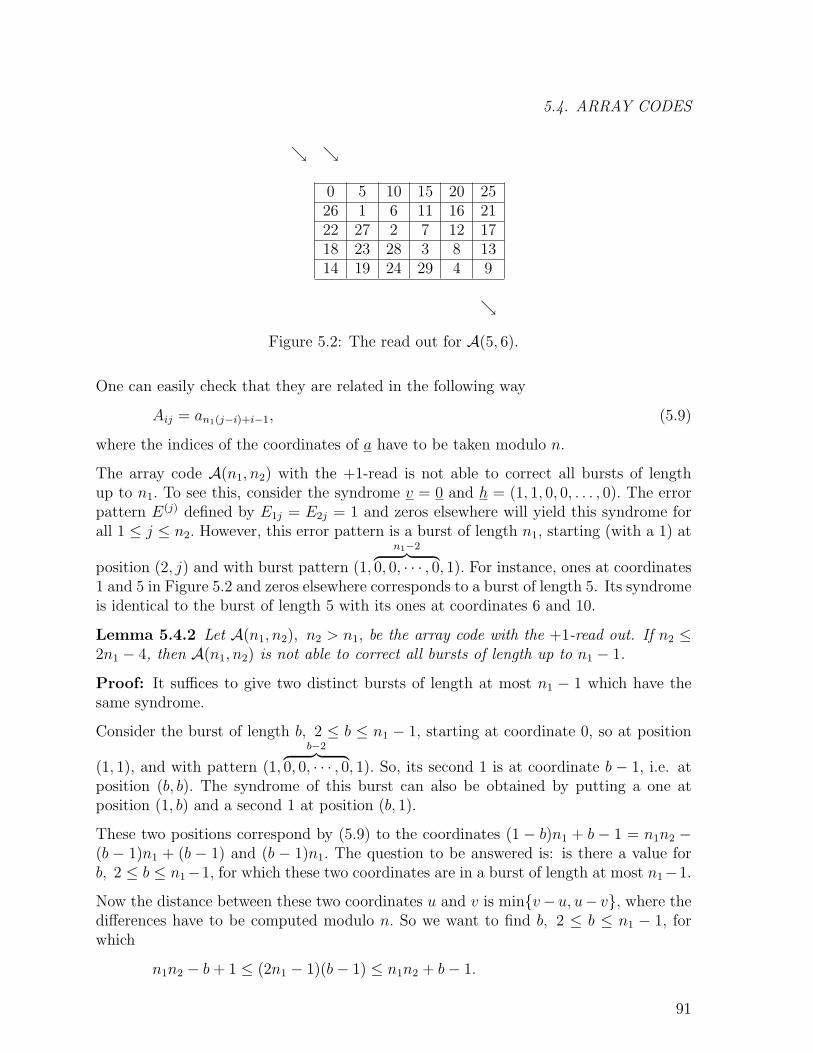
5.4. ARRAY CODES
↘ ↘
0 5 10 15 20 2526 1 6 11 16 2122 27 2 7 12 1718 23 28 3 8 1314 19 24 29 4 9
↘
Figure 5.2: The read out for A(5, 6).
One can easily check that they are related in the following way
Aij = an1(j−i)+i−1, (5.9)
where the indices of the coordinates of a have to be taken modulo n.
The array code A(n1, n2) with the +1-read is not able to correct all bursts of lengthup to n1. To see this, consider the syndrome v = 0 and h = (1, 1, 0, 0, . . . , 0). The errorpattern E(j) defined by E1j = E2j = 1 and zeros elsewhere will yield this syndrome forall 1 ≤ j ≤ n2. However, this error pattern is a burst of length n1, starting (with a 1) at
position (2, j) and with burst pattern (1,
n1−2︷ ︸︸ ︷0, 0, · · · , 0, 1). For instance, ones at coordinates
1 and 5 in Figure 5.2 and zeros elsewhere corresponds to a burst of length 5. Its syndromeis identical to the burst of length 5 with its ones at coordinates 6 and 10.
Lemma 5.4.2 Let A(n1, n2), n2 > n1, be the array code with the +1-read out. If n2 ≤2n1 − 4, then A(n1, n2) is not able to correct all bursts of length up to n1 − 1.
Proof: It suffices to give two distinct bursts of length at most n1 − 1 which have thesame syndrome.
Consider the burst of length b, 2 ≤ b ≤ n1 − 1, starting at coordinate 0, so at position
(1, 1), and with pattern (1,
b−2︷ ︸︸ ︷0, 0, · · · , 0, 1). So, its second 1 is at coordinate b − 1, i.e. at
position (b, b). The syndrome of this burst can also be obtained by putting a one atposition (1, b) and a second 1 at position (b, 1).
These two positions correspond by (5.9) to the coordinates (1 − b)n1 + b − 1 = n1n2 −(b − 1)n1 + (b − 1) and (b − 1)n1. The question to be answered is: is there a value forb, 2 ≤ b ≤ n1−1, for which these two coordinates are in a burst of length at most n1−1.
Now the distance between these two coordinates u and v is min{v−u, u− v}, where thedifferences have to be computed modulo n. So we want to find b, 2 ≤ b ≤ n1 − 1, forwhich
n1n2 − b+ 1 ≤ (2n1 − 1)(b− 1) ≤ n1n2 + b− 1.
91
CHAPTER 5. BURST CORRECTING CODES
This reduces to
n2 + 2
2≤ b ≤ n2 + 2
2+
n2
2(n1 − 1).
From n1 < n2, it follows that n2/(2(n1 − 1)) ≥ 1/2, so b = d(n2 + 2)/2e is a solution tothese inequalities.
Moreover, n2 ≤ 2n1−4 implies that (n2 +2)/2 ≤ n1−1, so b = d(n2 +2)/2e also satisfiesthe condition b ≤ n1 − 1.
2
Lemma 5.4.2 gives a necessary condition for the array code A(n1, n2), n2 > n1, to be(n1 − 1)-burst-correcting. This condition turns out to be sufficient.
Theorem 5.4.3 The array code A(n1, n2), n2 > n1, is (n1 − 1)-burst-correcting if andonly if n2 ≥ 2n1 − 3.
Instead of proving Theorem 5.4.3 directly we shall derive an extremely simple decodingalgorithm. In view of Lemma 5.4.2 we may assume that n2 ≥ 2n1 − 3.
Let R = C+B be a received word, where C is a codeword and B be a burst of length atmost n1− 1. Compute the syndromes h and v of R, which is the same as the syndromesof the burst B. We only need to discuss the case that h and v are not both equal to theall-zero vector.
It follows from the +1-read out that a burst of length n1 will affect each row or columnat most once. In other words, in the computation of the syndrome there will never bea cancelation of errors! Or, to say it differently, if hi = 1, there is exactly one error inthe i-th row and a row contains no errors if hi = 0. The same holds for the columns. Itfollows from this observation that h and v have the same Hamming weight, say w.
Next, view the coordinates of v cyclicly. Since the burst B affects at most n1 − 1consecutive columns, v will contain a gap of zeros of length at least n2− b ≥ n2−n1 +1.But there cannot be two gaps of length at least n2 − n1 + 1, because this would imply atotal number of coordinates of at least (n2 − n1 + 1) + 1 + (n2 − n1 + 1) + 1, which ismore than n2 under the condition n2 ≥ 2n1 − 3.
Let the coordinate immediately to the right of the gap be j1 (so vj1 = 1 and vj1−l = 0 for1 ≤ l ≤ (n2−n1 +1) and let the subsequent 1-coordinates in v have indices j2, j3, . . . , jw.Let 1 ≤ i1 < i2 < · · · < iw ≤ n1 denote the 1-coordinates in h.
We shall now show that the errors in B are at positions (il, jl), 1 ≤ l ≤ w. It suffices toshow that Ei1,j1 = 1.
Assume the contrary, so assume that Ei1,j1 = 0. It follows from hi = 0 for i < i1 thatthe error in column j1 is at a position (u, j1) with u > i1. Similarly it follows fromvj1−l = 0 for 1 ≤ l ≤ (n2 − n1 + 1) that the error in row i1 is at position (i1, v) with
92
5.4. ARRAY CODES
j1 < v ≤ j1 + n1 − 2, So, E(i1,j1) 6= 1 implies that E(u,j1) = 1 for some u ≥ i1 and thatE(i1,v) = 1 for some j1 ≤ v ≤ j1 + n1 − 2.
The proof will be finished by showing that the positions (u, j1) (i1, v) under these con-ditions will never lie in the same burst of length at most n1 − 1. The reason for this isthat the distance between these positions is at least n1− 1. Because the coordinates aretaken modulo n1n2, one needs to compute the minimum of two distances.
By (5.9)), these distances are
|n1n2 − {(v − i1)n1 + i1 − 1}+ {(j1 − u)n1 + u− 1}| =
|n1n2 − (v − j1)n1 − (u− i1)(n1 − 1)|.
and
|(v − j1)n1 + (u− i1)(n1 − 1)|.
The second expression is clearly always greater than or equal to n1 − 1. To prove thesame inequality for the first expression, we use that the inequalities on u and v implythat v− j1 ≤ n1− 2 and u− i1 ≤ n1− 1. So the first distance between the two positions(u, j1) and (i1, v) is at least
n1n2 − (n1 − 2)n1 − (n1 − 1)2,
which, by the inequality n2 ≥ 2n1 − 3, is at least
n1(2n1 − 3)− (n1 − 2)n1 − (n1 − 1)2 = n1 − 1.
So the two positions (u, j1) and (i1, v) with u > i1 and j1 < v ≤ j1 + n1 − 2 have actualdistance at least n1 − 1, so they are not in the same burst of length at most n1 − 1.
This proves the correctness of the following decoding algorithm.
Algorithm 5.4.4 (Decoding array codes) Let R(x) be the received word.
1. Compute the horizontal syndrome h defined by hi =∑
1≤j≤n2Rij =∑
1≤j≤n2Eij, 1 ≤ i ≤ n1 and the vertical syndrome v defined by vj =
∑1≤i≤n1
Rij =∑1≤i≤n1
Eij, 1 ≤ j ≤ n2.
2. Let 1 ≤ i1 < i2 < · · · < iw ≤ n1 denote the 1-coordinates in h.
3. Find the gap of length at least n2 − n1 + 1 in v, where the coordinates have to betaken modulo n2. Let the gap end at coordinate j1 − 1.
4. Let j1 < j2 < · · · < jw ≤ j1 + n1 − 2 denote the 1-coordinates in v.
5. The burst B(x) is one at the positions (il, jl), 1 ≤ l ≤ w and zero everywhere else.
6. C(x) = R(x) + B(x).
93
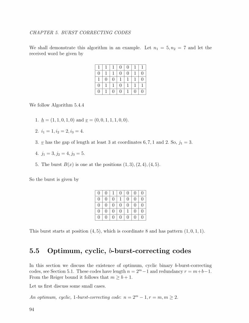
CHAPTER 5. BURST CORRECTING CODES
We shall demonstrate this algorithm in an example. Let n1 = 5, n2 = 7 and let thereceived word be given by
1 1 1 0 0 1 10 1 1 0 0 1 01 0 0 1 1 1 00 1 1 0 1 1 10 1 0 0 1 0 0
We follow Algorithm 5.4.4
1. h = (1, 1, 0, 1, 0) and v = (0, 0, 1, 1, 1, 0, 0).
2. i1 = 1, i2 = 2, i3 = 4.
3. v has the gap of length at least 3 at coordinates 6, 7, 1 and 2. So, j1 = 3.
4. j1 = 3, j2 = 4, j3 = 5.
5. The burst B(x) is one at the positions (1, 3), (2, 4), (4, 5).
So the burst is given by
0 0 1 0 0 0 00 0 0 1 0 0 00 0 0 0 0 0 00 0 0 0 1 0 00 0 0 0 0 0 0
This burst starts at position (4, 5), which is coordinate 8 and has pattern (1, 0, 1, 1).
5.5 Optimum, cyclic, b-burst-correcting codes
In this section we discuss the existence of optimum, cyclic binary b-burst-correctingcodes, see Section 5.1. These codes have length n = 2m−1 and redundancy r = m+b−1.From the Reiger bound it follows that m ≥ b+ 1.
Let us first discuss some small cases.
An optimum, cyclic, 1-burst-correcting code: n = 2m − 1, r = m,m ≥ 2.
94
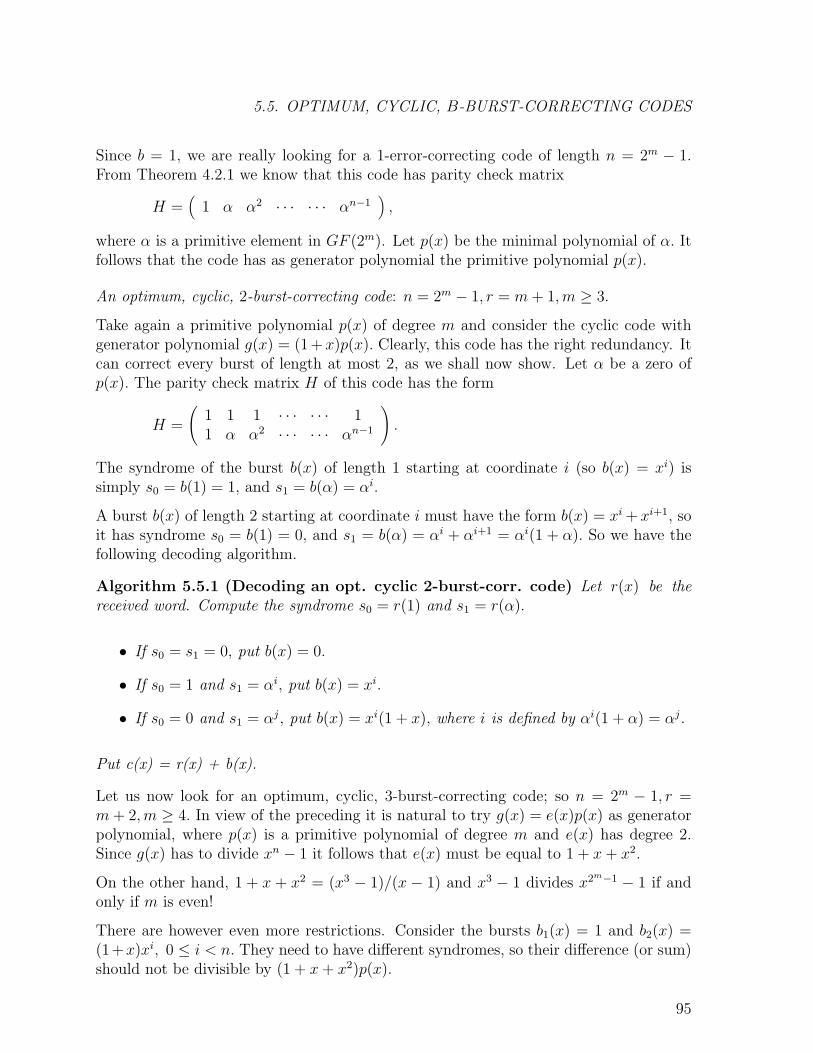
5.5. OPTIMUM, CYCLIC, B-BURST-CORRECTING CODES
Since b = 1, we are really looking for a 1-error-correcting code of length n = 2m − 1.From Theorem 4.2.1 we know that this code has parity check matrix
H =(
1 α α2 · · · · · · αn−1),
where α is a primitive element in GF (2m). Let p(x) be the minimal polynomial of α. Itfollows that the code has as generator polynomial the primitive polynomial p(x).
An optimum, cyclic, 2-burst-correcting code: n = 2m − 1, r = m+ 1,m ≥ 3.
Take again a primitive polynomial p(x) of degree m and consider the cyclic code withgenerator polynomial g(x) = (1+x)p(x). Clearly, this code has the right redundancy. Itcan correct every burst of length at most 2, as we shall now show. Let α be a zero ofp(x). The parity check matrix H of this code has the form
H =
(1 1 1 · · · · · · 11 α α2 · · · · · · αn−1
).
The syndrome of the burst b(x) of length 1 starting at coordinate i (so b(x) = xi) issimply s0 = b(1) = 1, and s1 = b(α) = αi.
A burst b(x) of length 2 starting at coordinate i must have the form b(x) = xi + xi+1, soit has syndrome s0 = b(1) = 0, and s1 = b(α) = αi + αi+1 = αi(1 + α). So we have thefollowing decoding algorithm.
Algorithm 5.5.1 (Decoding an opt. cyclic 2-burst-corr. code) Let r(x) be thereceived word. Compute the syndrome s0 = r(1) and s1 = r(α).
• If s0 = s1 = 0, put b(x) = 0.
• If s0 = 1 and s1 = αi, put b(x) = xi.
• If s0 = 0 and s1 = αj, put b(x) = xi(1 + x), where i is defined by αi(1 + α) = αj.
Put c(x) = r(x) + b(x).
Let us now look for an optimum, cyclic, 3-burst-correcting code; so n = 2m − 1, r =m+ 2,m ≥ 4. In view of the preceding it is natural to try g(x) = e(x)p(x) as generatorpolynomial, where p(x) is a primitive polynomial of degree m and e(x) has degree 2.Since g(x) has to divide xn − 1 it follows that e(x) must be equal to 1 + x+ x2.
On the other hand, 1 + x + x2 = (x3 − 1)/(x − 1) and x3 − 1 divides x2m−1 − 1 if andonly if m is even!
There are however even more restrictions. Consider the bursts b1(x) = 1 and b2(x) =(1+x)xi, 0 ≤ i < n. They need to have different syndromes, so their difference (or sum)should not be divisible by (1 + x+ x2)p(x).
95
CHAPTER 5. BURST CORRECTING CODES
Now, b1(x)+ b2(x) = 1+(1+x)xi, 1 ≤ i < n is divisible by 1+x+x2 = (x3−1)/(x−1)if and only if i ≡ 1 (mod 3). Thus, to make the code 3-burst-correcting, we have thefollowing necessary condition.
i ≡ 1 (mod 3) ⇒ (1 + x)xi 6≡ 1 (mod p(x)).
Since p(x) is a primitive polynomial, one can write 1 + x ≡ xa (mod p(x)) for some1 ≤ a ≤ n− 1. The condition above now reduces to
i ≡ 1 (mod 3) ⇒ xa+i 6≡ 1 (mod p(x)).
i.e.
i ≡ 1 (mod 3) ⇒ a+ i 6≡ 0 (mod 2m − 1).
Since 3|(2m − 1), one simply gets a 6≡ 2 (mod 3).
Of course we only checked possible problems with the burst patterns 1 and 1 + x. Onereally has to do this for all pairs of burst patterns, i.e. for all pairs of polynomials ofdegree less than 3, that have constant term 1. It turns out that no further conditions doarise. This proves:
Theorem 5.5.2 Let p(x) be a primitive polynomial of degree m. Then g(x) = (1 + x+x2)p(x) generates an optimum, cyclic 3-burst-correcting code if and only if
1. m is even,
2. a, defined by 1 + x ≡ xa (mod p(x)), is not congruent to 2 modulo 3.
Example 5.5.3 The cyclic code of length 15 generated by g(x) = (1+x+x2)(1+x+x4)is an optimum, 3-burst-correcting code, because 1 +x ≡ x4 (mod 1 +x+x4) and 4 6≡ 2(mod 3).
Questions that arise very naturally are:
• Is it necessary to start with g(x) = e(x)p(x), where p(x) is primitive of degree m?
• Are there always primitive polynomials p(x) of even degree m for which a 6≡ 2(mod 3), where 1 + x ≡ xa (mod p(x))?
• How to deal with b ≥ 4?
There are very satisfactory answers to all these questions and they will be given here.Unfortunatly, it leads too far to prove all these statements. The interested reader canfind the proofs in On the existence of optimum cyclic burst-correcting codes, K.A.S.Abdel-Ghaffar, e.o., IEEE Trans. Inform. Theory, vol. IT-32, pp.768-775, Nov. 1986.
Theorem 5.5.4 (Elspas-Short) If g(x) generates an optimum, cyclic b-burst-correcting code of length n = 2m − 1, then g(x) = e(x)p(x) with
96
5.6. PROBLEMS
1. degree(e(x)) = b− 1, e(0) = 1, e(x) has no multiple factors.
2. p(x) is a primitive polynomial of degree m,m ≥ b+1, where m is a multiple of me,defined as the smallest me with e(x)|(x2me−1 − 1).
All the conditions in the above theorem follow from the simple fact that g(x)|(xn − 1)(and the Reiger bound), except for the statement that g(x) contains a primitive factorof degree m.
Definition 5.5.5 The AES-conditions (short for Abramson-Elspas-Short conditions) onthe primitive polynomial p(x) in Theorem 5.5.4 are all the conditions that arise from
B1(x) ≡ xiB2(x) (mod e(x)) ⇒ B1(x) 6≡ xiB2(x) (mod p(x)),
for all 0 ≤ i < n and for all burst patterns B1(x) and B2(x) of degree at most b− 1 withB1(x) 6= B2(x) and both unequal to e(x).
Theorem 5.5.6 A polynomial g(x) generates an optimum, cyclic b-burst-correcting codeof length n = 2m − 1, if and only if it can be factored into g(x) = e(x)p(x) which satisfythe conditions in Theorem 5.5.4 and the AES-conditions.
Theorem 5.5.7 Let e(x) be a square-free polynomial of degree b−1 with e(0) = 1. Then,for all m sufficiently large and divisible by me, a primitive polynomial p(x) of degree mexists such that e(x)p(x) generates an optimum, cyclic b-burst-correcting code of lengthn = 2m − 1.
For two special cases even stronger results hold.
Theorem 5.5.8 For each even m,m ≥ 4, a primitive polynomial p(x) of degree m existssuch that (1+x+x2)p(x) generates an optimum, cyclic 3-burst-correcting code (of lengthn = 2m − 1).
Theorem 5.5.9 For each even m,m ≥ 10, a primitive polynomial p(x) of degree mexists such that (1 + x3)p(x) generates an optimum, cyclic 4-burst-correcting code (oflength n = 2m − 1).
The smallest degree primitive polynomial p(x) of degreem such that (1+x)(1+x+x3)p(x)generates an optimum, cyclic 5-burst-correcting code of length n = 2m − 1, is
p(x) = 1 + x+ x2 + x3 + x5 + x9 + x10 + x13 + x15.
5.6 Problems
5.6.1 By writing the coordinates of the words of an e-error-correcting, 16-ary Reed-Solomon code as binary words of length 4, one obtains a b-burst-correcting binarycode.
What should e be to get b = 9? And for b = 10?
97
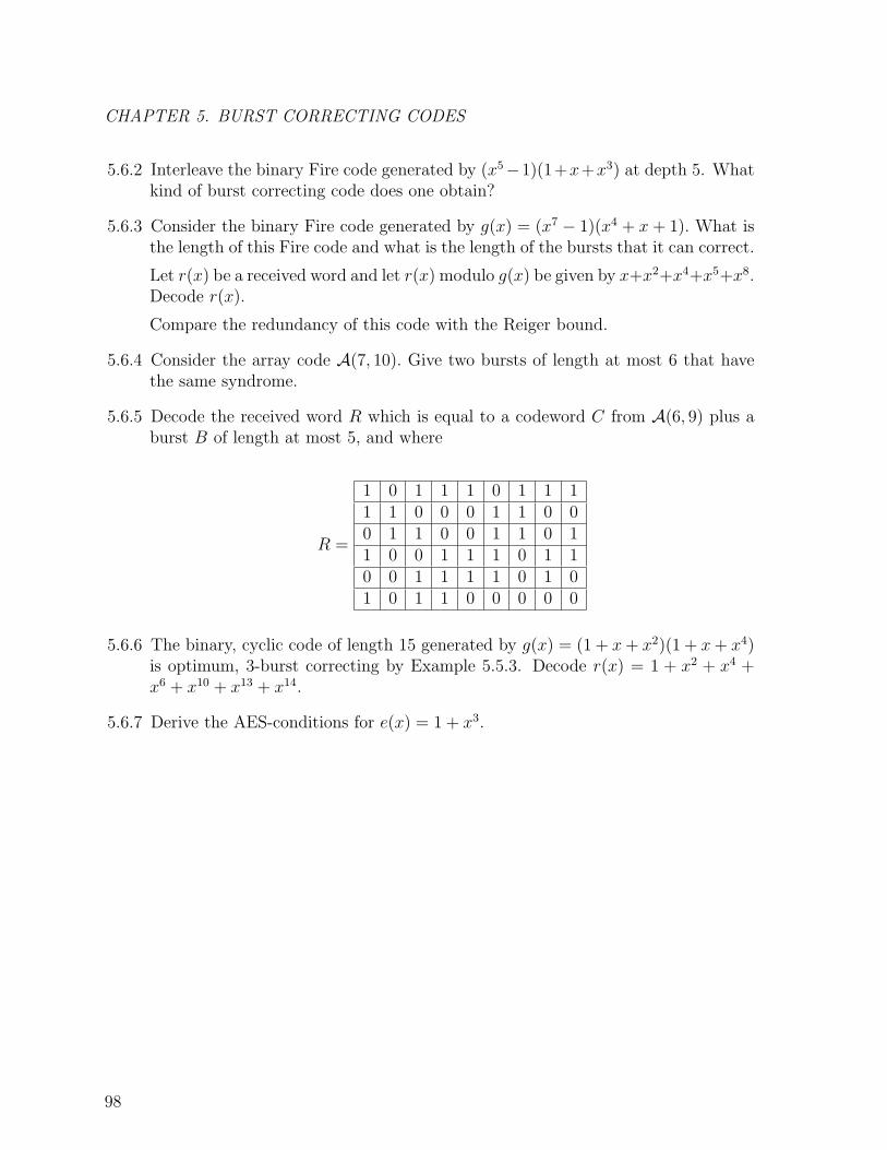
CHAPTER 5. BURST CORRECTING CODES
5.6.2 Interleave the binary Fire code generated by (x5−1)(1+x+x3) at depth 5. Whatkind of burst correcting code does one obtain?
5.6.3 Consider the binary Fire code generated by g(x) = (x7 − 1)(x4 + x+ 1). What isthe length of this Fire code and what is the length of the bursts that it can correct.
Let r(x) be a received word and let r(x) modulo g(x) be given by x+x2+x4+x5+x8.Decode r(x).
Compare the redundancy of this code with the Reiger bound.
5.6.4 Consider the array code A(7, 10). Give two bursts of length at most 6 that havethe same syndrome.
5.6.5 Decode the received word R which is equal to a codeword C from A(6, 9) plus aburst B of length at most 5, and where
R =
1 0 1 1 1 0 1 1 11 1 0 0 0 1 1 0 00 1 1 0 0 1 1 0 11 0 0 1 1 1 0 1 10 0 1 1 1 1 0 1 01 0 1 1 0 0 0 0 0
5.6.6 The binary, cyclic code of length 15 generated by g(x) = (1 + x+ x2)(1 + x+ x4)is optimum, 3-burst correcting by Example 5.5.3. Decode r(x) = 1 + x2 + x4 +x6 + x10 + x13 + x14.
5.6.7 Derive the AES-conditions for e(x) = 1 + x3.
98
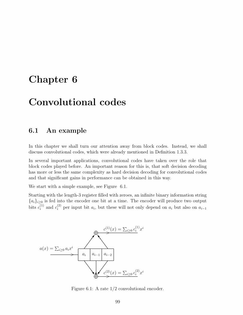
Chapter 6
Convolutional codes
6.1 An example
In this chapter we shall turn our attention away from block codes. Instead, we shalldiscuss convolutional codes, which were already mentioned in Definition 1.3.3.
In several important applications, convolutional codes have taken over the role thatblock codes played before. An important reason for this is, that soft decision decodinghas more or less the same complexity as hard decision decoding for convolutional codesand that significant gains in performance can be obtained in this way.
We start with a simple example, see Figure 6.1.
Starting with the length-3 register filled with zeroes, an infinite binary information string{ai}i≥0 is fed into the encoder one bit at a time. The encoder will produce two output
bits c(1)i and c
(2)i per input bit ai, but these will not only depend on ai but also on ai−1
⊕
⊕
>
>
>
ai ai−1 ai−2
��
��7
SS
SSo
SS
SSw
��
��/?
a(x) =∑
i≥0 aixi
c(2)(x) =∑
i≥0 c(2)i xi
c(1)(x) =∑
i≥0 c(1)i xi
Figure 6.1: A rate 1/2 convolutional encoder.
99
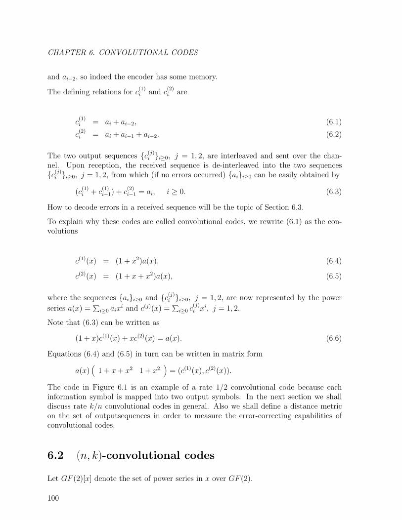
CHAPTER 6. CONVOLUTIONAL CODES
and ai−2, so indeed the encoder has some memory.
The defining relations for c(1)i and c
(2)i are
c(1)i = ai + ai−2, (6.1)
c(2)i = ai + ai−1 + ai−2. (6.2)
The two output sequences {c(j)i }i≥0, j = 1, 2, are interleaved and sent over the chan-nel. Upon reception, the received sequence is de-interleaved into the two sequences{c(j)i }i≥0, j = 1, 2, from which (if no errors occurred) {ai}i≥0 can be easily obtained by
(c(1)i + c
(1)i−1) + c
(2)i−1 = ai, i ≥ 0. (6.3)
How to decode errors in a received sequence will be the topic of Section 6.3.
To explain why these codes are called convolutional codes, we rewrite (6.1) as the con-volutions
c(1)(x) = (1 + x2)a(x), (6.4)
c(2)(x) = (1 + x+ x2)a(x), (6.5)
where the sequences {ai}i≥0 and {c(j)i }i≥0, j = 1, 2, are now represented by the power
series a(x) =∑
i≥0 aixi and c(j)(x) =
∑i≥0 c
(j)i xi, j = 1, 2.
Note that (6.3) can be written as
(1 + x)c(1)(x) + xc(2)(x) = a(x). (6.6)
Equations (6.4) and (6.5) in turn can be written in matrix form
a(x)(
1 + x+ x2 1 + x2)
= (c(1)(x), c(2)(x)).
The code in Figure 6.1 is an example of a rate 1/2 convolutional code because eachinformation symbol is mapped into two output symbols. In the next section we shalldiscuss rate k/n convolutional codes in general. Also we shall define a distance metricon the set of outputsequences in order to measure the error-correcting capabilities ofconvolutional codes.
6.2 (n, k)-convolutional codes
Let GF (2)[x] denote the set of power series in x over GF (2).
100
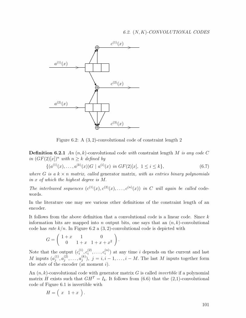
6.2. (N,K)-CONVOLUTIONAL CODES
⊕
⊕
⊕
>
>
>
>
>
����� 6
AAAAU ?
��
���
AAAAU
����� 6
a(1)(x)
a(2)(x)
c(1)(x)
c(2)(x)
c(3)(x)
Figure 6.2: A (3, 2)-convolutional code of constraint length 2
Definition 6.2.1 An (n, k)-convolutional code with constraint length M is any code Cin (GF (2)[x])n with n ≥ k defined by
{(a(1)(x), . . . , a(k)(x))G | a(i)(x) in GF (2)[x], 1 ≤ i ≤ k}, (6.7)
where G is a k × n matrix, called generator matrix, with as entries binary polynomialsin x of which the highest degree is M.
The interleaved sequences (c(1)(x), c(2)(x), . . . , c(n)(x)) in C will again be called code-words.
In the literature one may see various other definitions of the constraint length of anencoder.
It follows from the above definition that a convolutional code is a linear code. Since kinformation bits are mapped into n output bits, one says that an (n, k)-convolutionalcode has rate k/n. In Figure 6.2 a (3, 2)-convolutional code is depicted with
G =
(1 + x 1 0
0 1 + x 1 + x+ x2
).
Note that the output (c(1)i , c
(2)i , . . . , c
(n)i ) at any time i depends on the current and last
M inputs (a(1)j , a
(2)j , . . . , a
(k)j ), j = i, i − 1, . . . , i −M. The last M inputs together form
the state of the encoder (at moment i).
An (n, k)-convolutional code with generator matrix G is called invertible if a polynomialmatrix H exists such that GHT = Ik. It follows from (6.6) that the (2,1)-convolutionalcode of Figure 6.1 is invertible with
H =(x 1 + x
).
101
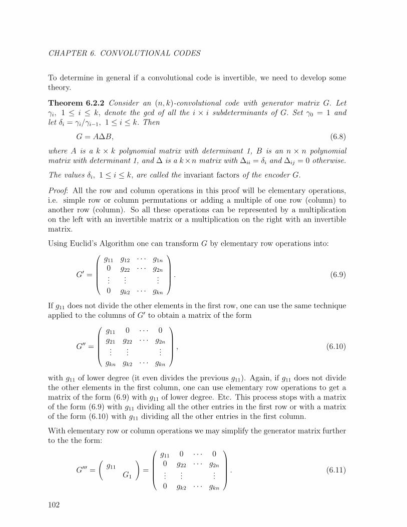
CHAPTER 6. CONVOLUTIONAL CODES
To determine in general if a convolutional code is invertible, we need to develop sometheory.
Theorem 6.2.2 Consider an (n, k)-convolutional code with generator matrix G. Letγi, 1 ≤ i ≤ k, denote the gcd of all the i × i subdeterminants of G. Set γ0 = 1 andlet δi = γi/γi−1, 1 ≤ i ≤ k. Then
G = A∆B, (6.8)
where A is a k × k polynomial matrix with determinant 1, B is an n × n polynomialmatrix with determinant 1, and ∆ is a k×n matrix with ∆ii = δi and ∆ij = 0 otherwise.
The values δi, 1 ≤ i ≤ k, are called the invariant factors of the encoder G.
Proof: All the row and column operations in this proof will be elementary operations,i.e. simple row or column permutations or adding a multiple of one row (column) toanother row (column). So all these operations can be represented by a multiplicationon the left with an invertible matrix or a multiplication on the right with an invertiblematrix.
Using Euclid’s Algorithm one can transform G by elementary row operations into:
G′ =
g11 g12 · · · g1n
0 g22 · · · g2n...
......
0 gk2 · · · gkn
. (6.9)
If g11 does not divide the other elements in the first row, one can use the same techniqueapplied to the columns of G′ to obtain a matrix of the form
G′′ =
g11 0 · · · 0g21 g22 · · · g2n...
......
gkn gk2 · · · gkn
, (6.10)
with g11 of lower degree (it even divides the previous g11). Again, if g11 does not dividethe other elements in the first column, one can use elementary row operations to get amatrix of the form (6.9) with g11 of lower degree. Etc. This process stops with a matrixof the form (6.9) with g11 dividing all the other entries in the first row or with a matrixof the form (6.10) with g11 dividing all the other entries in the first column.
With elementary row or column operations we may simplify the generator matrix furtherto the the form:
G′′′ =
(g11
G1
)=
g11 0 · · · 00 g22 · · · g2n...
......
0 gk2 · · · gkn
. (6.11)
102
6.2. (N,K)-CONVOLUTIONAL CODES
If one of the elements gij with i > 1 and j > 1 is not divisible by g11, we can addrow i to the top row. With elementary row and column operations one again arrives ata matrix of the form (6.11) but with g11 of lower degree. Repeating this process, onearrives at a generator matrix of the form (6.11) that has the property that g11 dividesall the elements in G1. Clearly g11 = δ1.
Similarly, G1 can be transformed into the form(δ2
G2
),
with δ1|δ2 and all elements in G2 divisible by δ2. Repeating this process yields the formin (6.8).
From the form (6.8) and the property δ1|δ2| · · · |δk, if follows that the gcd γi of all i × isubdeterminants of ∆ is equal to δ1δ2 · · · δi. Since the matrices A and B in (6.8) areproducts of elementary row resp. column operations, the same holds for subdeterminantsof G. So δi = γi/γi−1.
2
Since the matrices A and B in (6.8) are invertible, it follows from Theorem 6.2.2 that Gis invertible if and only if ∆ has a polynomial right inverse. This proves the followingcorollary.
Corollary 6.2.3 The generator matrix of a convolutional code is invertible if and onlyif all its invariant factors are equal to 1.
Write δk = xu(1+xv(x)) and assume that v(x) 6= 0. Then the input (0, 0, . . . , 11+xv(x)
)A−1
will result in xu times the k-th row of B as output. This means that this input of infiniteweight results in an output of finite weight (all terms in B are polynomials). This alsomeans that a finite set of errors during the transmission can result in the decoding to aninput that differs from the real input at infinitely many places. Such an encoder is calledcatastrophic. Clearly, one does not want to use catastrophic convolutional encoders.
On the other hand, assume that γk = xu. Note that if (c(1)(x), c(2)(x), . . . , c(n)(x)) hasfinitely many non-zero terms, then so does B−1(c(1)(x), c(2)(x), . . . , c(n)(x)). For thesame reason (a(1)(x), a(2)(x), . . . , a(k)(x))A cannot have finitely many non-zero terms,if (a(1)(x), a(2)(x), . . . , a(k)(x)) has infinitely many non-zero terms (A−1 has polynomialsas entries). But γk = xu implies that all γi’s (and consequently all δi’s) are powers ofx. Thus (a(1)(x), a(2)(x), . . . , a(k)(x))A has infinitely many non-zero terms implies thatB−1(c(1)(x), c(2)(x), . . . , c(n)(x)) cannot have finitely many non-zero terms. It followsthat the encoder cannot be catastrophic in this case.
The discussion above proves the following theorem.
Theorem 6.2.4 The encoder of an (n, k)-convolutional code with invariant factorsγ1|γ2| · · · |γk is catastrophic if and only if γk is not a power of x.
103
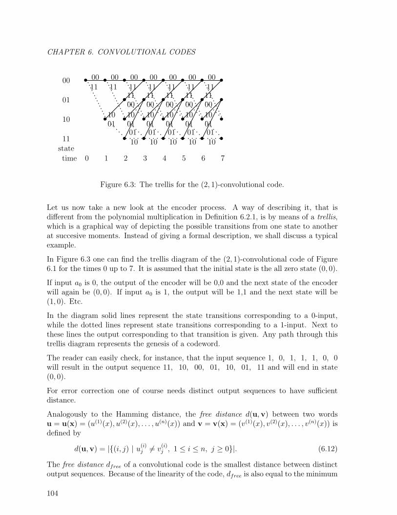
CHAPTER 6. CONVOLUTIONAL CODES
• • • • • • • •
• • • • • •
• • • • • • •
• • • • • •
00 00 00 00 00 00 0011 11 11 11 11 11 11
11 11 11 11 1100 00 00 00 00
10 10 10 10 10 1001 01 01 01 01 01
01 01 01 01 0110 10 10 10 10
��
�
��
�
��
�
��
�
��
�
��
�
��
�
��
�
��
�
��
�
��
�
������
������
������
������
������
················
················
················
················
················
················
················
········
········
········
········
················
········
········
········
········
········· · · · · · · · · · · · · · · · · · · · · · · · ·
00
01
10
11state
time 0 1 2 3 4 5 6 7
Figure 6.3: The trellis for the (2, 1)-convolutional code.
Let us now take a new look at the encoder process. A way of describing it, that isdifferent from the polynomial multiplication in Definition 6.2.1, is by means of a trellis,which is a graphical way of depicting the possible transitions from one state to anotherat succesive moments. Instead of giving a formal description, we shall discuss a typicalexample.
In Figure 6.3 one can find the trellis diagram of the (2, 1)-convolutional code of Figure6.1 for the times 0 up to 7. It is assumed that the initial state is the all zero state (0, 0).
If input a0 is 0, the output of the encoder will be 0,0 and the next state of the encoderwill again be (0, 0). If input a0 is 1, the output will be 1,1 and the next state will be(1, 0). Etc.
In the diagram solid lines represent the state transitions corresponding to a 0-input,while the dotted lines represent state transitions corresponding to a 1-input. Next tothese lines the output corresponding to that transition is given. Any path through thistrellis diagram represents the genesis of a codeword.
The reader can easily check, for instance, that the input sequence 1, 0, 1, 1, 1, 0, 0will result in the output sequence 11, 10, 00, 01, 10, 01, 11 and will end in state(0, 0).
For error correction one of course needs distinct output sequences to have sufficientdistance.
Analogously to the Hamming distance, the free distance d(u,v) between two wordsu = u(x) = (u(1)(x), u(2)(x), . . . , u(n)(x)) and v = v(x) = (v(1)(x), v(2)(x), . . . , v(n)(x)) isdefined by
d(u,v) = |{(i, j) | u(i)j 6= v
(i)j , 1 ≤ i ≤ n, j ≥ 0}|. (6.12)
The free distance dfree of a convolutional code is the smallest distance between distinctoutput sequences. Because of the linearity of the code, dfree is also equal to the minimum
104
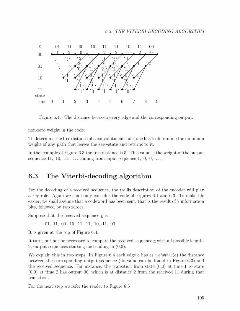
6.3. THE VITERBI-DECODING ALGORITHM
• • • • • • • • • •
• • • • • • •
• • • • • • •
• • • • • •
��
�
��
�
��
�
��
�
��
�
��
�
��
�
��
�
��
�
��
�
��
�
��
�
��
�
��
�
������
������
������
������
������
������
················
················
················
················
················
················
················
········
········
········
········
················
········
········
········
········
········· · · · · · · · · · · · · · · · · · · · · · · · ·
00
01
10
11state
time
r 01 11 00 10 11 11 10 11 00
0 1 2 3 4 5 6 7 8 9
11
20
11
0 12 12 10 1
1 01 21 21 0
2 20 00 02 2
1 11 11 11 1
1 211 01
0 122 10
0
2
Figure 6.4: The distance between every edge and the corresponding output.
non-zero weight in the code.
To determine the free distance of a convolutional code, one has to determine the minimumweight of any path that leaves the zero-state and returns to it.
In the example of Figure 6.3 the free distance is 5. This value is the weight of the outputsequence 11, 10, 11, . . . coming from input sequence 1, 0, 0, . . . .
6.3 The Viterbi-decoding algorithm
For the decoding of a received sequence, the trellis description of the encoder will playa key role. Again we shall only consider the code of Figures 6.1 and 6.3. To make lifeeasier, we shall assume that a codeword has been sent, that is the result of 7 informationbits, followed by two zeroes.
Suppose that the received sequence r is
01, 11, 00, 10, 11, 11, 10, 11, 00.
It is given at the top of Figure 6.4.
It turns out not be necessary to compare the received sequence r with all possible length-9, output sequences starting and ending in (0,0).
We explain this in two steps. In Figure 6.4 each edge e has as weight w(e) the distancebetween the corresponding output sequence (its value can be found in Figure 6.3) andthe received sequence. For instance, the transition from state (0,0) at time 1 to state(0,0) at time 2 has output 00, which is at distance 2 from the received 11 during thattransition.
For the next step we refer the reader to Figure 6.5
105
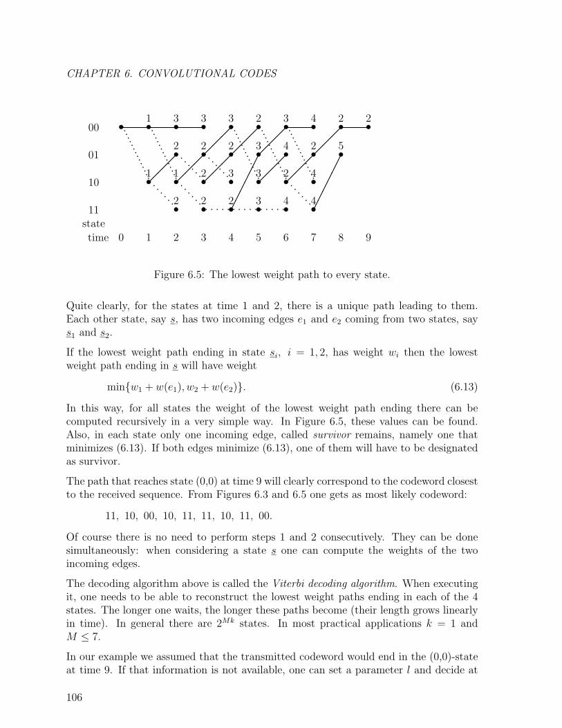
CHAPTER 6. CONVOLUTIONAL CODES
• • • • • • • • • •
• • • • • • •
• • • • • • •
• • • • • •
················
················��
�
········
········��
�
········
��
�
��
�········
· · · · ·
��
�
������
················
· · · · ·
��
�
��
�
················
· · · · ·
��
�
························
��
�
������
00
01
10
11state
time
1
1
3
2
1
2
3
2
2
2
3
2
3
2
2
3
3
3
3
4
2
4
4
2
4
4
2
5
2
0 1 2 3 4 5 6 7 8 9
Figure 6.5: The lowest weight path to every state.
Quite clearly, for the states at time 1 and 2, there is a unique path leading to them.Each other state, say s, has two incoming edges e1 and e2 coming from two states, says1 and s2.
If the lowest weight path ending in state si, i = 1, 2, has weight wi then the lowestweight path ending in s will have weight
min{w1 + w(e1), w2 + w(e2)}. (6.13)
In this way, for all states the weight of the lowest weight path ending there can becomputed recursively in a very simple way. In Figure 6.5, these values can be found.Also, in each state only one incoming edge, called survivor remains, namely one thatminimizes (6.13). If both edges minimize (6.13), one of them will have to be designatedas survivor.
The path that reaches state (0,0) at time 9 will clearly correspond to the codeword closestto the received sequence. From Figures 6.3 and 6.5 one gets as most likely codeword:
11, 10, 00, 10, 11, 11, 10, 11, 00.
Of course there is no need to perform steps 1 and 2 consecutively. They can be donesimultaneously: when considering a state s one can compute the weights of the twoincoming edges.
The decoding algorithm above is called the Viterbi decoding algorithm. When executingit, one needs to be able to reconstruct the lowest weight paths ending in each of the 4states. The longer one waits, the longer these paths become (their length grows linearlyin time). In general there are 2Mk states. In most practical applications k = 1 andM ≤ 7.
In our example we assumed that the transmitted codeword would end in the (0,0)-stateat time 9. If that information is not available, one can set a parameter l and decide at
106
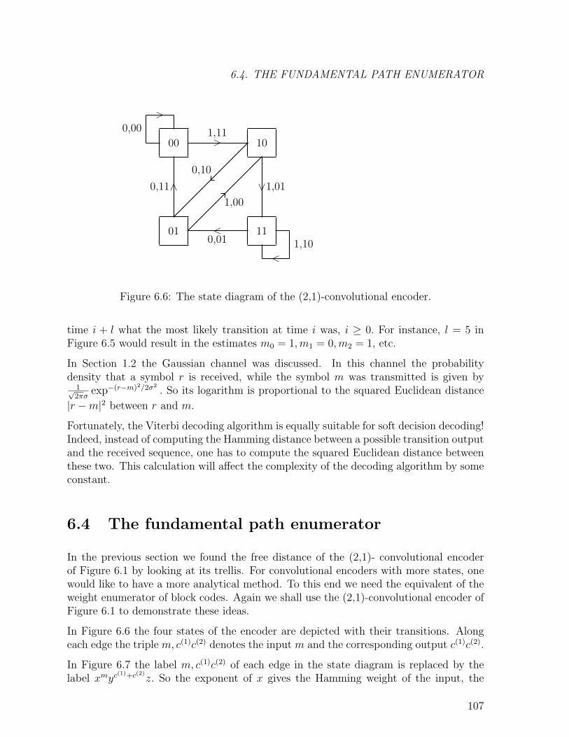
6.4. THE FUNDAMENTAL PATH ENUMERATOR
01 11
00 10
��
��
��
��
��
��
��
��
1,11>
0,01<
1,01∨0,11∧
1,10
<
0,00>
0,10
1,00
Figure 6.6: The state diagram of the (2,1)-convolutional encoder.
time i + l what the most likely transition at time i was, i ≥ 0. For instance, l = 5 inFigure 6.5 would result in the estimates m0 = 1,m1 = 0,m2 = 1, etc.
In Section 1.2 the Gaussian channel was discussed. In this channel the probabilitydensity that a symbol r is received, while the symbol m was transmitted is given by
1√2πσ
exp−(r−m)2/2σ2. So its logarithm is proportional to the squared Euclidean distance
|r −m|2 between r and m.
Fortunately, the Viterbi decoding algorithm is equally suitable for soft decision decoding!Indeed, instead of computing the Hamming distance between a possible transition outputand the received sequence, one has to compute the squared Euclidean distance betweenthese two. This calculation will affect the complexity of the decoding algorithm by someconstant.
6.4 The fundamental path enumerator
In the previous section we found the free distance of the (2,1)- convolutional encoderof Figure 6.1 by looking at its trellis. For convolutional encoders with more states, onewould like to have a more analytical method. To this end we need the equivalent of theweight enumerator of block codes. Again we shall use the (2,1)-convolutional encoder ofFigure 6.1 to demonstrate these ideas.
In Figure 6.6 the four states of the encoder are depicted with their transitions. Alongeach edge the triple m, c(1)c(2) denotes the input m and the corresponding output c(1)c(2).
In Figure 6.7 the label m, c(1)c(2) of each edge in the state diagram is replaced by thelabel xmyc(1)+c(2)z. So the exponent of x gives the Hamming weight of the input, the
107
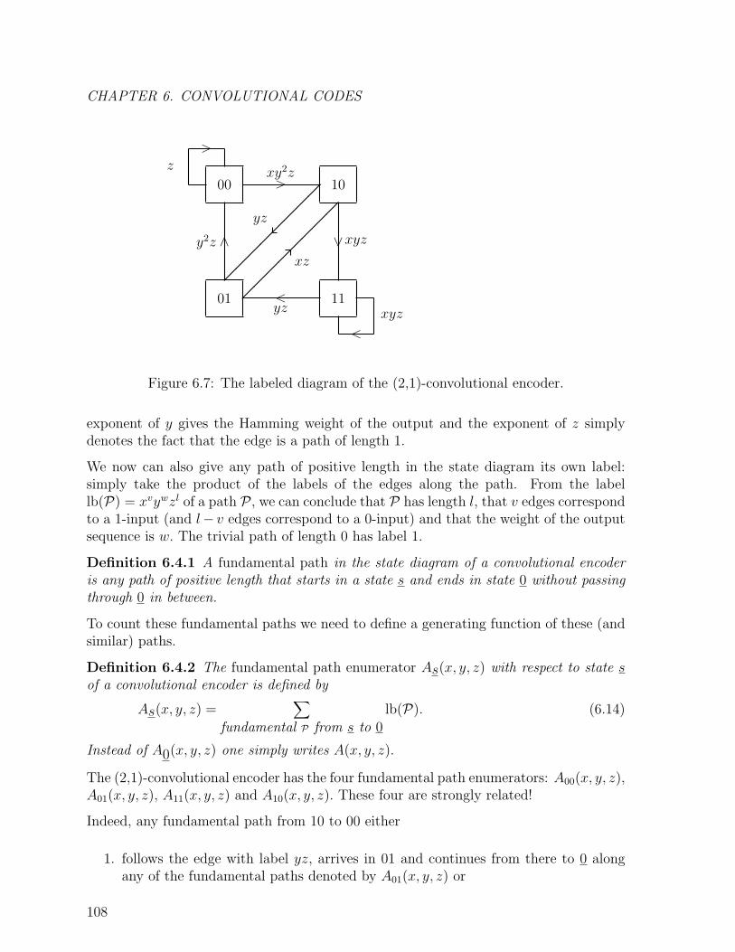
CHAPTER 6. CONVOLUTIONAL CODES
01 11
00 10
��
��
��
��
��
��
��
��
xy2z>
yz<
xyz∨y2z ∧
xyz
<
z>
yz
xz
Figure 6.7: The labeled diagram of the (2,1)-convolutional encoder.
exponent of y gives the Hamming weight of the output and the exponent of z simplydenotes the fact that the edge is a path of length 1.
We now can also give any path of positive length in the state diagram its own label:simply take the product of the labels of the edges along the path. From the labellb(P) = xvywzl of a path P , we can conclude that P has length l, that v edges correspondto a 1-input (and l− v edges correspond to a 0-input) and that the weight of the outputsequence is w. The trivial path of length 0 has label 1.
Definition 6.4.1 A fundamental path in the state diagram of a convolutional encoderis any path of positive length that starts in a state s and ends in state 0 without passingthrough 0 in between.
To count these fundamental paths we need to define a generating function of these (andsimilar) paths.
Definition 6.4.2 The fundamental path enumerator As(x, y, z) with respect to state sof a convolutional encoder is defined by
As(x, y, z) =∑
fundamental P from s to 0lb(P). (6.14)
Instead of A0(x, y, z) one simply writes A(x, y, z).
The (2,1)-convolutional encoder has the four fundamental path enumerators: A00(x, y, z),A01(x, y, z), A11(x, y, z) and A10(x, y, z). These four are strongly related!
Indeed, any fundamental path from 10 to 00 either
1. follows the edge with label yz, arrives in 01 and continues from there to 0 alongany of the fundamental paths denoted by A01(x, y, z) or
108
6.4. THE FUNDAMENTAL PATH ENUMERATOR
2. follows the edge with label xyz, arrives in 11 and continues from there to 0 alongany of the fundamental paths denoted by A11(x, y, z).
So we have the relation
A10(x, y, z) = yzA01(x, y, z) + xyzA11(x, y, z).
In the same way, one can find the relations
A00(x, y, z) = xy2zA10(x, y, z),
A01(x, y, z) = y2z + xzA10(x, y, z),
A11(x, y, z) = yzA01(x, y, z) + xyzA11(x, y, z).
This gives rise to the following matrix equation:
1 0 −xy2z 00 1 −xz 00 −yz 1 −xyz0 −yz 0 1− xyz
A00(x, y, z)A01(x, y, z)A10(x, y, z)A11(x, y, z)
=
0y2z00
.(6.15)
From equation (6.15) it is now simple to determine A0,0(x, y, z) (use Kramer’s Rule).
A0,0(x, y, z) =
∣∣∣∣∣∣∣∣∣0 0 −xy2z 0y2z 1 −xz 00 −yz 1 −xyz0 −yz 0 1− xyz
∣∣∣∣∣∣∣∣∣∣∣∣∣∣∣∣∣∣1 0 −xy2z 00 1 −xz 00 −yz 1 −xyz0 −yz 0 1− xyz
∣∣∣∣∣∣∣∣∣
,
and thus
A0,0(x, y, z) =xy5z3
1− xyz − xyz2=
xy5z3
1− xyz(1 + z). (6.16)
From xy5z3
1−xyz(1+z)= xy5z3{1 + xyz(1 + z) + (xyz(1 + z))2 + · · · } it follows that the
fundamental path with lowest output weight (i.e. with the smallest exponent of y) hasweight 5. In other words the free distance of this convolutional encoder is 5.
It also follows that there is only one fundamental path with output weight 5, since thereis only one term with y5, namely xy5z3, and its coefficient is 1. The exponent 1 of x
109
CHAPTER 6. CONVOLUTIONAL CODES
and the exponent 3 of z in xy5z3 tell that this fundamental path is caused by a single1-input and that it has length 3 (so there were two 0-inputs).
Just like the weight enumerator of a cyclic code can be used to estimate the probablityof incorrect decoding (see the end of Section 2.3), the fundamental path enumeratorA(x, y, z) turns out to be very helpful when studying various error probabilities thatone may want to evaluate. Here, we shall only give an upper bound on the so-calledfirst error probability i.e. the probability that the decoder makes an error right at thebeginning. By the linearity, this means that we are calculating the probability thatstarting in the zero state, only zeroes inputs have occurred, while the decoder finds oneof the fundamental paths more likely.
Let Pre(P ; 0) denote the probability that fundamental path P is a more likely transmit-ted sequence, while in fact the all-zero sequence was transmitted.
The first error probablity Pr1 is bounded above by∑fundamental P
from 0
Pre(P ; 0). (6.17)
For the BSC with error probability p, the probability Pre(P ; 0) only depends on theHamming weight w of the output sequence corresponding to P :
Pre(P ; 0) =∑
k≥dw/2e
(w
k
)pk(1− p)w−k.
From ∑k≥dw/2e
(w
k
)pk(1− p)w−k ≤ pw/2(1− p)w/2
∑k≥dw/2e
(w
k
)≤
≤ pw/2(1− p)w/22w =
=(2√p(1− p)
)w
it follows that
Pr1 ≤∑
fundamentalP from 0
(2√p(1− p))w(P) = A(1, 2
√p(1− p), 1).
This proves the following theorem.
Theorem 6.4.3 The first error probablity Pr1 of a convolutional encoder with funda-mental path enumerator A(x, y, z) satisfies
Pr1 ≤ A(1, 2√p(1− p), 1). (6.18)
110
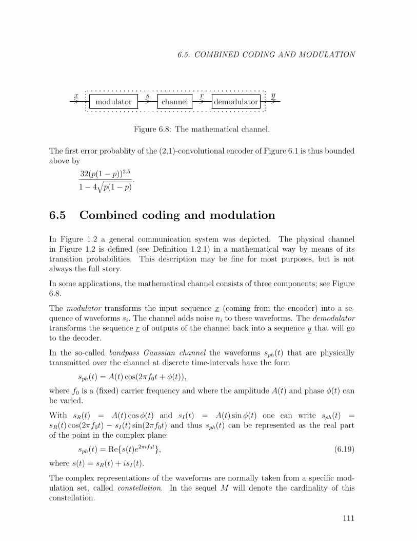
6.5. COMBINED CODING AND MODULATION
modulator channel demodulator> >> >x ys r· · · · · · · · · · · · · · · · · · · · · · · · · · · · · · · · · · · · · · · · · · · ·
· · · · · · · · · · · · · · · · · · · · · · · · · · · · · · · · · · · · · · · · · · · ·········
········
Figure 6.8: The mathematical channel.
The first error probablity of the (2,1)-convolutional encoder of Figure 6.1 is thus boundedabove by
32(p(1− p))2.5
1− 4√p(1− p)
.
6.5 Combined coding and modulation
In Figure 1.2 a general communication system was depicted. The physical channelin Figure 1.2 is defined (see Definition 1.2.1) in a mathematical way by means of itstransition probabilities. This description may be fine for most purposes, but is notalways the full story.
In some applications, the mathematical channel consists of three components; see Figure6.8.
The modulator transforms the input sequence x (coming from the encoder) into a se-quence of waveforms si. The channel adds noise ni to these waveforms. The demodulatortransforms the sequence r of outputs of the channel back into a sequence y that will goto the decoder.
In the so-called bandpass Gaussian channel the waveforms sph(t) that are physicallytransmitted over the channel at discrete time-intervals have the form
sph(t) = A(t) cos(2πf0t+ φ(t)),
where f0 is a (fixed) carrier frequency and where the amplitude A(t) and phase φ(t) canbe varied.
With sR(t) = A(t) cosφ(t) and sI(t) = A(t) sinφ(t) one can write sph(t) =sR(t) cos(2πf0t) − sI(t) sin(2πf0t) and thus sph(t) can be represented as the real partof the point in the complex plane:
sph(t) = Re{s(t)e2πif0t}, (6.19)
where s(t) = sR(t) + isI(t).
The complex representations of the waveforms are normally taken from a specific mod-ulation set, called constellation. In the sequel M will denote the cardinality of thisconstellation.
111
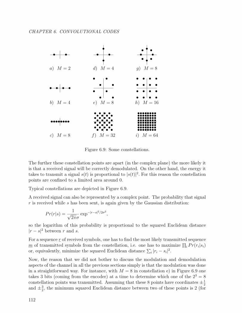
CHAPTER 6. CONVOLUTIONAL CODES
••••••••
• • • •
• •
••••••••••••••••••••••••••••••••••••••••••••••••••••••••••••••••
• • • •• • • •• • • •• • • •
• ••
•
•
•
•
•• ••
•
• •• •• •
• •
• • • •• • • •• • • •• • • •• • • •• • • •• • • •• • • •
c) M = 8 f) M = 32
b) M = 4 e) M = 8
a) M = 2 d) M = 4
i) M = 64
h) M = 16
g) M = 8
Figure 6.9: Some constellations.
The further these constellation points are apart (in the complex plane) the more likely itis that a received signal will be correctly demodulated. On the other hand, the energy ittakes to transmit a signal s(t) is proportional to |s(t)|2. For this reason the constellationpoints are confined to a limited area around 0.
Typical constellations are depicted in Figure 6.9.
A received signal can also be represented by a complex point. The probability that signalr is received while s has been sent, is again given by the Gaussian distribution:
Pr(r|s) =1√2πσ
exp−|r−s|2/2σ2
,
so the logarithm of this probability is proportional to the squared Euclidean distance|r − s|2 between r and s.
For a sequence r of received symbols, one has to find the most likely transmitted sequencem of transmitted symbols from the constellation, i.e. one has to maximize
∏i Pr(ri|si)
or, equivalently, minimize the squared Euclidean distance∑
i |ri − si|2.
Now, the reason that we did not bother to discuss the modulation and demodulationaspects of the channel in all the previous sections simply is that the modulation was donein a straightforward way. For instance, with M = 8 in constellation e) in Figure 6.9 onetakes 3 bits (coming from the encoder) at a time to determine which one of the 23 = 8constellation points was transmitted. Assuming that these 8 points have coordinates ±1
2
and ±32, the minimum squared Euclidean distance between two of these points is 2 (for
112
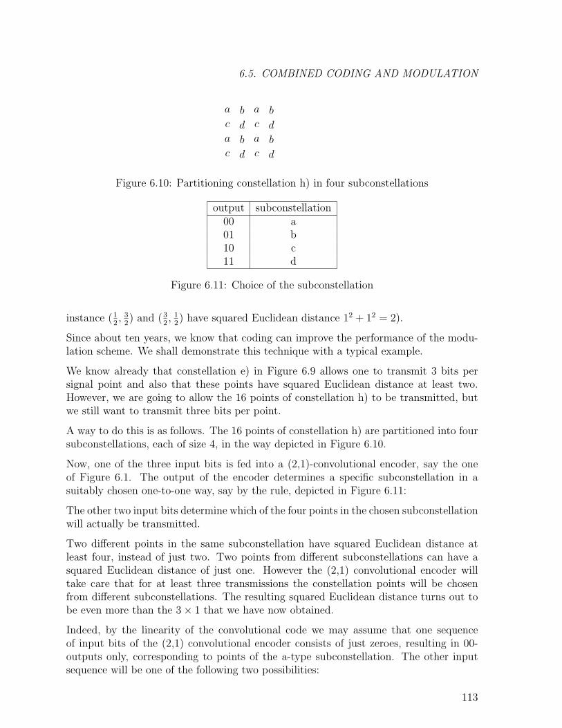
6.5. COMBINED CODING AND MODULATION
d d
a ad d
a a
c cb b
c cb b
Figure 6.10: Partitioning constellation h) in four subconstellations
output subconstellation00 a01 b10 c11 d
Figure 6.11: Choice of the subconstellation
instance (12, 3
2) and (3
2, 1
2) have squared Euclidean distance 12 + 12 = 2).
Since about ten years, we know that coding can improve the performance of the modu-lation scheme. We shall demonstrate this technique with a typical example.
We know already that constellation e) in Figure 6.9 allows one to transmit 3 bits persignal point and also that these points have squared Euclidean distance at least two.However, we are going to allow the 16 points of constellation h) to be transmitted, butwe still want to transmit three bits per point.
A way to do this is as follows. The 16 points of constellation h) are partitioned into foursubconstellations, each of size 4, in the way depicted in Figure 6.10.
Now, one of the three input bits is fed into a (2,1)-convolutional encoder, say the oneof Figure 6.1. The output of the encoder determines a specific subconstellation in asuitably chosen one-to-one way, say by the rule, depicted in Figure 6.11:
The other two input bits determine which of the four points in the chosen subconstellationwill actually be transmitted.
Two different points in the same subconstellation have squared Euclidean distance atleast four, instead of just two. Two points from different subconstellations can have asquared Euclidean distance of just one. However the (2,1) convolutional encoder willtake care that for at least three transmissions the constellation points will be chosenfrom different subconstellations. The resulting squared Euclidean distance turns out tobe even more than the 3× 1 that we have now obtained.
Indeed, by the linearity of the convolutional code we may assume that one sequenceof input bits of the (2,1) convolutional encoder consists of just zeroes, resulting in 00-outputs only, corresponding to points of the a-type subconstellation. The other inputsequence will be one of the following two possibilities:
113
CHAPTER 6. CONVOLUTIONAL CODES
i) There is a single 1-input (all others are 0) in the second sequence. In this case theoutput sequence of the (2,1) convolutional encoder looks like:
· · · , 00, 00, 11, 10, 11, 00, 00, · · · ,
corresponding to the sequence of subconstellations
· · · , a , a , d , c , d , a , a , · · · .
So, in this case the squared Euclidean distance between the two sequences of constellationpoints is at least 2 + 1 + 2 = 5.
ii) There are more than one 1-inputs. The output sequence of the (2,1) convolutionalencoder will differ in at least four steps from the output sequence coming from the all-zero input sequence. So, during at least four consecutive transmissions, points will bechosen from different constellations, resulting in a squared Euclidean distance of at least4.
Taking the minimum of all possibilities, we conclude that this specific combined codingand modulation scheme has increased the minimum squared Euclidean distance from 2to 4. In practical situations this already gives rise to a considerable increase in reliability.
6.6 Problems
6.6.1 Decode the received sequence
11, 11, 00, 11, 10, 01, 00, 11, 10
in Figure 6.3, if the transmitted codeword can be assumed to be the result of 7information symbols followed by 2 zeroes.
6.6.2 Determine the invariant factors of the (5,3)-convolutional code with generatormatrix
G =
1 1 + x 1 + x2 1 1 + x+ x2
1 + x 1 + x x+ x3 0 x+ x3
x x+ x2 1 + x+ x2 + x3 x 1 + x+ x3
.6.6.3 Let C be the (2,1)-convolutional code generated by
G =(
1 + x 1 + x2).
Give an input sequence with infinitely many non-zero elements resulting in anoutput with finitely many non-zero elements.
Determine the path enumerator of this code.
114
6.6. PROBLEMS
6.6.4 Make the trellis for the (2,1)-convolutional code C generated by
G =(
1 + x+ x3 1 + x+ x2 + x3).
What is the free distance of C?
6.6.5 Assume that the points in Figure 6.10 have coordinates ±12
and ±32
and let thefour points x1, x2, x3, x4 in each of the four subconstellations
x3
x1
x4
x2
be the image of two of the three information bits in the following way:
00 → x1
01 → x2
11 → x3
10 → x4
.
The choice of the particular subconstellation is made according to the rule inFigure 6.11 by the output of the convolutional code of Figure 6.1, which has thethird information bit as input.
Decode the received sequence
· · · , a1, a1, d2, c3, d4, a1, a1, · · · .
115

CHAPTER 6. CONVOLUTIONAL CODES
116

6.6. PROBLEMS
115

CHAPTER . CONVOLUTIONAL CODES
116

Appendix A
Finite fields
All readers are assumed to be familiar with Q, R, and C, the sets of rational, realand complex numbers. These sets have nice properties with respect to addition andmultiplication, properties that will be extensively discussed in this appendix. Thesethree sets are examples of so-called fields.
In the context of coding theory fields of finite cardinality play a crucial role. This is sobecause most codes consist of vectors taken from a vector space over a finite field and,secondly, many good codes are constructed by algebraic methods. In this appendix anintroduction will be given to the theory of finite fields. All possible results regardingfinite fields that are needed in the chapters can be found in this appendix.
A.1 The integers
Let N denote the set of natural numbers and Z the set of integers. If an integer d dividesan integer n, i.e. n = k · d for some k ∈ Z, this will be denoted by d | n. If d does notdivide n one writes d|/n.
An integer p, p > 1, is said to be prime, if it has no other positive divisors than 1 andp. It is already known since Euclid (300 B.C.) that there exist infinitely many primenumbers. With p1 = 2, p2 = 3, p3 = 5, etc., a natural numbering of the primes is given.
Definition A.1.1 The greatest common divisor of two integers a and b, denoted bygcd(a, b) or (a, b), is the, uniquely determined, greatest positive integer dividing both aand b, so
gcd(a, b) = max{d > 0 | (d | a) ∧ (d | b)}. (A.1)
Similarly the least common multiple of two integers a and b, denoted by lcm[a, b] or [a, b],is the, uniquely determined, least positive integer divisible by both a and b, so
lcm[a, b] = min{m > 0 | (a | m) ∧ (b | m)}. (A.2)
117
APPENDIX A. FINITE FIELDS
The next theorem follows directly from an algorithm that will be presented below.
Theorem A.1.2 Let a and b be in N . Then there exist integers u and v such that
ua+ vb = gcd(a, b). (A.3)
Let a and b be two positive integers with b ≥ a. Clearly any divisor of a and b is a divisorof a and b− a and vice versa. It follows that gcd(a, b) = gcd(a, b− a) and for the samereason that gcd(a, b) = gcd(r, a), where r is defined by usual “division with remainder”,i.e. b = q · a+ r, 0 ≤ r < a. If r = 0, one may conclude that gcd(a, b) = a, while if r > 0one can continue in exactly the same way with a and r. This method gives an extremelyfast way of computing the gcd of a and b. The next algorithm shows how to find u andv satisfying (A.3) in an efficient way.
Algorithm A.1.3 (Euclid’s algorithm)
(initialize) s0 = b; s1 = a;
u0 = 0; u1 = 1;
v0 = 1; v1 = 0;
n = 1;
while sn > 0 do
begin n = n+ 1; qn = bsn−2/sn−1c;
sn = sn−2 − qnsn−1;
(so sn is the remainder of sn−2 divided by sn−1)
un = qnun−1 + un−2;
vn = qnvn−1 + vn−2
end;
u = (−1)nun−1; v = (−1)n−1vn−1; (A.4)
gcd(a, b) = sn−1. (A.5)
Proof: Since the numbers sn, n ≥ 1, form a strictly decreasing sequence of nonnegativeintegers, the algorithm will terminate after at most b iterations (in fact it will terminatemuch faster; see Problems A.6.1 and A.6.2).
From the relation sn = sn−2 − qnsn−1 in the algorithm and the argument given belowTheorem A.1.2 it follows that
gcd(a, b) = gcd(s0, s1) = gcd(s1, s2) = · · · == gcd(sn−1, sn) = gcd(sn−1, 0) = sn−1.
118

A.1. THE INTEGERS
This proves (A.5). Next we want to prove that for all k, 0 ≤ k ≤ n,
(−1)k−1uka+ (−1)kvkb = sk. (A.6)
For k = 0 and k = 1 (A.6) is true by the initialization values of u0, u1, v0, and v1. Weproceed by induction. It follows from the relations given in the algorithm and from theinduction hypothesis that
sk = sk−2 − qksk−1 =
{(−1)k−3uk−2a+ (−1)k−2vk−2b} − qk{(−1)k−2uk−1a+ (−1)k−1vk−1b} =
= (−1)k−1{uk−2 + qkuk−1}a+ (−1)k{vk−2 + qkvk−1}b =
= (−1)k−1uka+ (−1)kvkb.
This proves (A.6) for all k, 0 ≤ k ≤ n. Substitution of k = n− 1 in (A.6) yields
(−1)nun−1a+ (−1)n−1vn−1b = sn−1. (A.7)
Comparison of (A.7) with (A.3) proves the identities in (A.4).
2
Theorem A.1.2 makes it possible to prove elementary properties of numbers.
Corollary A.1.4 Let a, b, and d be integers such that d divides ab. Then gcd(d, a) = 1implies that d | b.
Proof: Theorem A.1.2 applied to a and d shows the existence of integers u and v suchthat 1 = ua + vd. Multiplication of this relation by b yields b = u(ab) + (vb)d. Since ddivides both ab and d, it follows that d also divides u(ab) + (vb)d, i.e. b.
2
It is now quite easy to prove (see Problem A.6.3) the following theorem.
Theorem A.1.5 (Fundamental Theorem of Number Theory)Any positive integer has a unique factorization of the form∏
ipei
i , ei ∈ N . (A.8)
Let a =∏
i peii , ei ∈ N , and b =
∏i p
fii , fi ∈ N . Then
gcd(a, b) =∏
ip
min{ei,fi}i , (A.9)
lcm[a, b] =∏
ip
max{ei,fi}i , (A.10)
gcd(a, b) · lcm[a, b] = ab. (A.11)
119
APPENDIX A. FINITE FIELDS
A special function on N that will be needed in Section A.5 will be defined next.
Definition A.1.6 (Euler’s Totient Function) The function φ(m) is defined as thenumber of integers less than or equal to m that are coprime with m, so
φ(m) =| {1 ≤ r ≤ m | gcd(r,m) = 1} | . (A.12)
Theorem A.1.7 For all positive integers n∑d|nφ(d) = n. (A.13)
Proof: Let d | n. By writing k = id one sees immediately that the number of elementsk, 1 ≤ k ≤ n, with gcd(k, n) = d is equal to the number of integers i with 1 ≤ i ≤ n/dand gcd(i, n/d) = 1. So this number is φ(n/d). On the other hand, gcd(k, n) divides nfor each integer k, 1 ≤ k ≤ n. It follows that
∑d|n φ(n/d) =
∑d|n∑
1≤k≤n,gcd(k,n)=d 1 =∑1≤k≤n 1 = n, which is equivalent to (A.13).
2
Let p be a prime number. Since every integer r, 1 ≤ r < p, has gcd 1 with p, it followsthat φ(p) = p − 1. Also φ(pe), p prime, can easily be evaluated. Indeed, since only themultiples of p have a nontrivial factor in common with pe, one has:
φ(pe) = pe − pe−1 = pe−1(p− 1) = pe(1− 1
p). (A.14)
If m = pe11 p
e22 with both p1 and p2 prime and both e1 and e2 positive, one can again
easily evaluate φ(m). In this case m/p1 integers in between 1 and m are a multiple of p1,m/p2 integers in between 1 and m are a multiple of p2, but m/p1p2 of these integers area multiple of both p1 and p2 (namely the multiples of p1p2). It follows that in this case
φ(m) = φ(pe11 p
e22 ) = m− m
p1
− m
p2
+m
p1p2
= m(1− 1
p1
)(1− 1
p2
).
Generalizing this (by means of the Principle of Inclusion and Exclusion) one obtains inthis way the following theorem.
Theorem A.1.8
φ(m) = m ·∏
p prime, p|m(1− 1
p). (A.15)
Two integers a and b are said to be congruent to each other modulo m, if their differenceb− a is divisible by m. This so-called congruence relation is denoted by:
a ≡ b (mod m). (A.16)
For instance 25 ≡ 3 (mod 11) since 11|(25− 3). In this terminology one also has 5 + 8 ≡ 2(mod 11) and 5× 9 ≡ 1 (mod 11).
Lemma A.1.9 Let ka ≡ kb (mod m) and gcd(k,m) = 1. Then a ≡ b (mod m).
120
A.2. RELATIONS
Proof: Since ka− kb = xm, x ∈ Z, and gcd(m, k) = 1, it follows from Corollary A.1.4that m | (a− b), i.e. a ≡ b (mod m).
2
The simplest congruence, and one that one often has to solve, is the so-called linearcongruence relation:
ax ≡ b (mod m). (A.17)
Theorem A.1.10 The linear congruence relation ax ≡ b (mod m) has a solution x forevery a, 1 ≤ a ≤ m − 1 and every b if and only if m is a prime. If m is a prime, saym = p, this solution is unique modulo p.
Proof: If m is composite, say m = m1m2 with 1 < m1 < m, the congruence relationm1x ≡ 1 (mod m) obviously does not have a solution, since both m and xm1 are divisibleby m1, but 1 is not.
If m is a prime p, the sets {0, 1, . . . , p−1} and {0a, 1a, . . . , (p−1)a} are the same modulop by Lemma A.1.9. In particular each element b in the first set can be written in a uniqueway as a product ax (modulo p) in the second set. It follows that the congruence relationax ≡ b (mod p) has a unique solution modulo p.
2
The solution of ax ≡ b (mod p), 1 ≤ a ≤ p − 1, can easily be found with Euclid’sAlgorithm. Indeed, from ua + vp = 1 (see (A.3)), it follows that ua ≡ 1 (mod p). Sothe solution x of the congruence relation ax ≡ b (mod p) is given by bu (mod p), sincea(bu) ≡ b(ua) ≡ b (mod p). One often writes a−1 for the unique element u satisfying ua≡ 1 (mod p).
Example A.1.11 To solve 17x ≡ 16 (mod 37), one first applies Euclid’s Algorithm to17 and 37. One gets (−13)× 17 + 6× 37 = 1. So 24× 17 ≡ (−13)× 17 ≡ 1 (mod 37).
It follows that 17−1 ≡ 24 (mod 37) and that the solution of 17x ≡16 (mod 37) is given by x ≡ 17−1 × 16 ≡ 24× 16 ≡ 14 (mod 37).
A.2 Relations
The congruence relation defined in (A.16) is a special case of a concept that will bedefined next.
Definition A.2.1 Let S be any set and let U be a non-empty subset of S × S. Then Udefines a relation ∼ on S by
∀s,t∈S [s ∼ t iff (s, t) ∈ U ]. (A.18)
121
APPENDIX A. FINITE FIELDS
An equivalence relation is a relation with the additional properties:
reflexivity: ∀s∈S [s ∼ s] (E1)
symmetry: ∀s,t∈S [(s ∼ t)⇒ (t ∼ s)] (E2)
transitivity: ∀s,t,u∈S [(s ∼ t ∧ t ∼ u)⇒ (s ∼ u)] (E3)
Let S be the set of straight lines in the (Euclidean) plane. Then “being parallel or equal”defines an equivalence relation. In Section A.1 we have seen another example. There, arelation (called congruence relation, see (A.16)) was defined on S = Z by a ≡ b (mod m)iff m | (a− b). The reader can easily check that this congruence relation indeed satisfies(E1), (E2) and (E3) and thus is an equivalence relation (see also Problem A.6.4).
An equivalence relation ∼ on a set S partitions S into so-called equivalence classes < s >defined by
< s >= {t ∈ S | t ∼ s}, (A.19)
So < s > consists of those elements in S that are equivalent to s. It is straightforwardto check that for any equivalence class < s > one has
i) ∀t,u∈<s> [t ∼ u],ii) ∀t∈<s> ∀u∈S\<s> [¬(t ∼ u)].
The equivalence classes of the congruence relation defined in (A.16) are called congruenceclasses. The set of congruence classes of the integers modulo m will be denoted by Zm.Its elements are < 0 >, < 1 >, . . . , < m − 1 > but will often simply be represented bythe numbers 0, 1, . . . ,m− 1.
A.3 Algebra
In this section sets will be discussed with operations defined on them that are similar tothe + and × defined on the reals.
Let S be a nonempty set. Any mapping from S × S into S is called an operation on S.The image of the pair (s, t) under this operation will, for the moment, be denoted bys ∗ t. An operation ∗ is called commutative if
∀s,t∈S [s ∗ t = t ∗ s]. (A.20)
An element e in S that satisfies
∀s∈S [s ∗ e = e ∗ s = s], (A.21)
will be called a unit-element of (S, ∗). If (S, ∗) has a unit-element, it is be unique. Indeed,suppose that e and e′ both satisfy (A.21). Then by (A.21) e = e ∗ e′ = e′.
122
A.3. ALGEBRA
Example A.3.1 Consider the operation + (i.e. addition) defined on Z. This operationis commutative and (Z,+) has 0 as unit-element.
Example A.3.2 Let S be the set of 2× 2 integer matrices. Multiplication of matricesis not a commutative operation. Consider for instance(
1 10 1
)(0 11 0
)=
(1 11 0
)6=(
0 11 1
)=
(0 11 0
)(1 10 1
).
This set S does however have a unit-element, namely(1 00 1
).
When applying the same operation repeatedly one often does not like the outcome todepend on the order in which the operations were executed. In other words one does notwant to need brackets in expressions like s ∗ t ∗ u. An operation ∗ is called associative, if
∀s,t,u∈S [s ∗ (t ∗ u) = (s ∗ t) ∗ u]. (A.22)
Example A.3.3 The operation ∧ defined on the positive integers by s ∧ t = st (so ∧stands for “raising to the power”) is not associative as follows from
(2 ∧ 3) ∧ 2 = (23)2 = 26 6= 29 = 2(32) = 2 ∧ (3 ∧ 2).
Definition A.3.4 Let G be a nonempty set and ∗ an operation defined on G. Then thepair (G, ∗) is called a group, if
operation ∗ is associative, (G1)
G contains a unit-element, say e, (G2)
∀g∈G ∃h∈G [g ∗ h = h ∗ g = e]. (G3)
The uniqueness of the element h in (G3) can be seen quite easily. Indeed, if h and h′
both satisfy (G3), then h = h ∗ e = h ∗ (g ∗ h′) = (h ∗ g) ∗ h′ = e ∗ h′ = h′. The elementh satisfying (G3) is called the inverse of g, and will be denoted by g−1.
A group (G, ∗) is called commutative, if the operation ∗ is commutative. The readereasily checks that (Z,+) in Example A.3.1 is a commutative group. Other well-knownexamples of commutative groups are for instance (Q,+), (Q \ {0}, ·), (R,+), etc.
Example A.3.2 does not yield a group, because not all matrices have an inverse (e.g. theall-one matrix).
On the set Zm defined at the end of Section A.2 one can define two operations (calledaddition and multiplication) that coincide with the modular arithmetic explained in(A.16):
< s > + < t >:=< s+ t >, s, t ∈ Z, (A.23)
< s > × < t >:=< st >, s, t ∈ Z. (A.24)
The proof of the next lemma is left as an exercise (Problem A.6.5).
123
APPENDIX A. FINITE FIELDS
Lemma A.3.5 The set Zm together with the addition +, as defined in (A.23), is acommutative group with < 0 > as unit-element.
Lemma A.3.6 The set Z∗m = Zm \ {< 0 >} together with the multiplication ×, as
defined in (A.24), is a group if and only if m is a prime p. In this case (Z∗p ,×) is
commutative and has < 1 > as unit-element.
Proof: Clearly (Z∗m,×) satisfies properties (G1) and (G2). That it satisfies (G3) if and
only if m is a prime is a direct consequence of Theorem A.1.10.
2
If (G, ∗) is a group and G contains a non-empty subset H such that (H, ∗) is also agroup one calls (H, ∗) a subgroup of (G, ∗). Because associativity already holds for theoperation ∗, (H, ∗) will be a subgroup of (G, ∗) iff
the product of any two elements in H also lies in H, (H1)
the unit-element e of (G, ∗) lies in H, (H2)
the inverse of an element of H also lies in H. (H3)
It is left as an exercise (see Problem A.6.6) to check that (H2) and (H3) are equivalentto
∀g,h∈H [g ∗ h−1 ∈ H]. (H)
Let m ∈ Z \ {0}. Then (mZ,+), where mZ is the set of all integer multiples of m, somZ = {mk | k ∈ Z}, is a commutative subgroup of (Z,+), as one can easily check.
We shall now consider the situation where two operations are defined on a set. (The firstwill be denoted by g + h, the second by g × h, g · h or just gh.)
Definition A.3.7 The triple (R,+,×) is called a ring, if
(R,+) is a commutative group (R1)
(its unit-element will be denoted by 0),
the operation × is associative, (R2)
distributivity holds, i.e. (R3)
∀r,s,t∈R [r(s+ t) = rs+ rt and (r + s)t = rt+ st].
The (additive) inverse of an element r in the group (R,+) will be denoted by −r, just as2r denotes r+ r, 3r denotes r+ r+ r, etc. Note that 0 really behaves like a zero-element,because for every r ∈ R one has that 0r = (r − r)r = r2 − r2 = 0 and similarly thatr0 = 0.
Suppose that the (multiplicative) operation × is commutative on R. Then the ring(R,+,×) will be called commutative. Examples of commutative rings are (Z,+, ·),
124
A.3. ALGEBRA
(Q,+, ·), (R,+, ·) and (Zm,+, ·), m 6= 0. Also mZ, the set of m-tuples, with the sameaddition and multiplication as in (Z,+, ·) forms a commutative ring.
Let (R,+,×) be a ring and S ⊂ R, such that (S,+,×) is also a ring. Then (S,+,×)is called a subring. Clearly (Q,+, ·) is a subring of (R,+, ·). The ring (mZ,+, ·) is asubring of (Z,+, ·).
Later the following special class of subrings will play an important role.
Definition A.3.8 A subring (I,+,×) of a ring (R,+,×) is called an ideal, if
∀i∈I ∀r∈R [ir ∈ I and ri ∈ I]. (I)
It is easy to check that an integer multiple of a multiple of m, m ∈ Z \ {0}, is alsoa multiple of m.. From this observation it follows that (mZ,+, ·) forms an ideal in(Z,+, ·).
In a ring (R,+,×) the element 0 obviously can not have a multiplicative inverse, unlessR consists of the single element 0. Indeed, suppose that r0 = e, for some r ∈ R. Thenfor each x ∈ R one has that x = xe = x(r0) = (xr)0 = 0, i.e. R = {0}.
It is however quite possible that (R∗,×) with R∗ = R \ {0} has the structure of a group.
Definition A.3.9 A triple (F,+,×) is called a field, if
(F,+) is a commutative group (F1)
(its unit-element is denoted by 0),
(F \ {0},×) is a group (F2)
(the multiplicative unit-element is denoted by e),
distributivity holds. (F3)
The multiplicative inverse of an element a in a field will be denoted by a−1.
Examples of fields are the rationals (Q,+,×), the reals (R,+,×) and the complex num-bers (C,+,×).
Unlike some rings, a field can not have so-called zero-divisors, i.e. elements a and b, bothunequal to 0, whose product ab equals 0. Indeed, suppose that ab = 0 and a 6= 0. Thenb = e× b = (a−1a)b = a−1(ab) = a−10 = 0.
If a subring (K,+,×) of a field (F,+,×) also has the structure of a field, we shall call(K,+,×) a subfield of (F,+,×).
In the sequel we shall be interested in a so-called finite groups (G, ∗), finite rings (R,+,×)and finite fields (F,+,×) of order n, meaning that G, resp. R and F are (finite) sets ofcardinality n.
Analogously to rings we define a commutative field (F,+, ·) to be a field, for which themultiplication is commutative. The following theorem will not be proved.
125
APPENDIX A. FINITE FIELDS
Theorem A.3.10 (Wedderburn) Every finite field is commutative.
In this appendix we shall study the structure of finite fields. It will turn out that finitefields of order q only exist when q is a prime power. Moreover these finite fields areessentially unique for a given size q. This justifies the widely accepted notation Fq orGF (q) (where GF stands for Galois Field after the Frenchman Galois) for a finite fieldof order q. Examples of finite fields will follow in Section A.4.
Before we conclude this section, some additional properties of finite groups need to bederived.
Let (G, ·) be a finite multiplicative group with unit-element e and let g be a nonzeroelement in G. Let g2, g3, etc., denote g × g, g × g × g, etc. Also, let g0 denote theunit-element e. Consider the sequence of elements e, g, g2, . . . in G. Since G is finite,there exists a unique integer n such that the elements e, g, . . . , gn−1 are all different, whilegn = gj for some j, 0 ≤ j < n. It follows that gn+1 = gj+1, etc. If j > 0, it would alsofollow that gn−1 = gj−1, contradicting the assumption on n. We conclude that j = 0, i.e.gn = e. So the elements gi, 0 ≤ i ≤ n− 1, are all distinct and gn = e.
It is now clear that the elements e, g, . . . , gn−1 form a subgroupH inG. Such a (sub)groupH is called a cyclic (sub)group of order n. We say that the element g generates H andthat g has order n.
Lemma A.3.11 Let (G, ·) be a group and g an element in G of order n. Then for all m
gm = e iff n divides m.
Proof: Write m = qn+ r, 0 ≤ r < n. Then gm = e iff gr = e, i.e. iff r = 0, i.e. iff n | m.
2
Lemma A.3.12 Let (G, ·) be a group and g an element in G of order n. Then elementgk, k > 0, has order n/ gcd(k, n).
Proof: Let m be the order of gk. Since k/ gcd(k, n) is integer, it follows that
(gk)n/ gcd(k,n) = (gn)k/ gcd(k,n) = (e)k/ gcd(k,n) = e.
From Lemma A.3.11 we conclude that m divides n/ gcd(k, n). To prove the converse, weobserve that (gk)m = e. Lemma A.3.11 implies that n divides km. Hence n/ gcd(k, n)divides m.
2
It follows from Definition A.1.6 that exactly φ(n) powers of an element g of order n inG will have order n.
Corresponding to a subgroup (H, ·) of a finite group (G, ·) an equivalence relation ∼ on
126
A.4. CONSTRUCTIONS
G can be defined (see Problem A.6.8) by
a ∼ b iff ab−1 ∈ H. (A.25)
The equivalence classes are of the form {ha | h ∈ H}, as one can easily check. Theyall have the same cardinality as H. It follows that the number of equivalence classes is| G | / | H | . As a consequence | H | divides | G | . This proves the following theorem.
Theorem A.3.13 Let (G, ·) be a finite group of order n. Then every subgroup (H, ·) of(G, ·) has an order dividing n. Also every element g, g 6= e in G has an order dividing n.
A.4 Constructions
Let (R,+,×) be a commutative ring with (multiplicative) unit-element e. Let (S,+,×)be an ideal in (R,+,×). The relation ≡ on R will be defined by
∀a,b∈R [a ≡ b (mod R) iff a− b ∈ S]. (A.26)
It is a simple exercise to check that (A.26) defines an equivalence relation on R. WithR/S (read: R modulo S) the set of equivalence classes will be denoted. As before < a >will stand for the class containing a, so < a >= {a+s | s ∈ S}. Based on the operationsin R, one defines in R/S
< a > + < b >:=< a+ b >, a, b ∈ R, (A.27)
< a > × < b >:=< ab >, a, b ∈ R, (A.28)
It is necessary to verify that these definitions are independent of the particular choiceof the elements a and b in the equivalence classes < a > resp. < b > . Again it is veryelementary to check the following theorem.
Theorem A.4.1 Let (R,+,×) be a commutative ring with unit-element e and let(S,+,×) be an ideal in (R,+,×). With the above definitions (R/S,+,×) is a com-mutative ring with unit-element < e > .
The ring (R/S,+,×), defined above, is called a residue class ring. It is instrumental inconstructing finite fields.
Since (mZ,+, ·) is an ideal in the commutative ring (Z,+, ·), one can with Theorem A.4.1also describe the ring (Zm,+, ·) as the residue class ring (Z/mZ,+, ·). This residue classring is commutative and has < 1 > as multiplicative unit-element.
Theorem A.4.2 Let m be a positive integer. The ring (Zm,+, ·) is a finite field withm elements if and only if m is prime.
127
APPENDIX A. FINITE FIELDS
Proof: By Lemma A.3.5 the commutative ring (Zm,+, ·) (with m elements) satisfiesproperty (F1). Also (F3) holds trivially.
The statement now follows directly from Lemma A.3.6. 2
In the next section it will be shown that for p prime, (Zp,+, ·) is essentially the onlyfield with p elements.
Our next goal is to to construct finite fields of size q, where q = pm, p prime.
Let (F,+, ·) be a commutative field (not necessarily finite). Then F [x] denotes the setof polynomials over F, i.e. the set of expressions
f(x) =∑n
i=0fix
i = f0 + f1x+ · · ·+ fnxn, (A.29)
for some n in N , where the fi, 0 ≤ i ≤ n, lie in F and are called the coefficients of f(x).Unless f0 = f1 = . . . = fn = 0 one can assume without loss of generality that fn 6= 0.This integer n is called the degree of f(x).
Addition and multiplication of polynomials is defined in the obvious way.∑n
i=0fix
i +∑n
i=0gix
i =∑n
i=0(fi + gi)x
i. (A.30)
(∑m
i=0fix
i) (∑n
j=0gjx
j)
=∑m+n
k=0
(∑i+j=k
figj
)xk. (A.31)
It is now straightforward to verify the next theorem.
Theorem A.4.3 Let (F,+, ·) be a commutative field. Then (F [x],+, ·) is a commutativering with unit-element.
What will be done now for F [x] will be completely analogous to what has been done forZ in the previous sections. For that reason, not all arguments will be repeated.
So, in F [x] the following notions can be defined: divisibility, reducibility (if a polynomialcan be written as the product of two polynomials of lower degree), irreducibility (whichis the analog of primality), the greatest common divisor gcd, the least common multiplelcm, a unique factorization theorem (the analog of Theorem A.1.5), Euclid’s Algorithm,congruence relations, etc. Note that the gcd and lcm are now uniquely determined upto a multiplication by a constant.
In particular we have the following theorem and corollary (see also (A.3) and TheoremA.1.10).
Theorem A.4.4 Let a(x) and b(x) be polynomials in F [x]. Then there exist polynomialsu(x) and v(x) in F [x], such that
u(x)a(x) + v(x)b(x) = gcd(a(x), b(x)). (A.32)
128
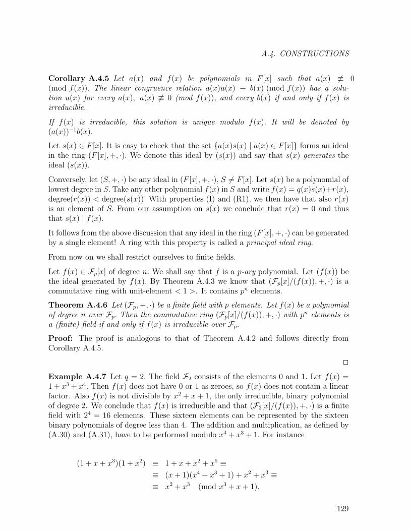
A.4. CONSTRUCTIONS
Corollary A.4.5 Let a(x) and f(x) be polynomials in F [x] such that a(x) 6≡ 0(mod f(x)). The linear congruence relation a(x)u(x) ≡ b(x) (mod f(x)) has a solu-tion u(x) for every a(x), a(x) 6≡ 0 (mod f(x)), and every b(x) if and only if f(x) isirreducible.
If f(x) is irreducible, this solution is unique modulo f(x). It will be denoted by(a(x))−1b(x).
Let s(x) ∈ F [x]. It is easy to check that the set {a(x)s(x) | a(x) ∈ F [x]} forms an idealin the ring (F [x],+, ·). We denote this ideal by (s(x)) and say that s(x) generates theideal (s(x)).
Conversely, let (S,+, ·) be any ideal in (F [x],+, ·), S 6= F [x]. Let s(x) be a polynomial oflowest degree in S. Take any other polynomial f(x) in S and write f(x) = q(x)s(x)+r(x),degree(r(x)) < degree(s(x)). With properties (I) and (R1), we then have that also r(x)is an element of S. From our assumption on s(x) we conclude that r(x) = 0 and thusthat s(x) | f(x).
It follows from the above discussion that any ideal in the ring (F [x],+, ·) can be generatedby a single element! A ring with this property is called a principal ideal ring.
From now on we shall restrict ourselves to finite fields.
Let f(x) ∈ Fp[x] of degree n. We shall say that f is a p-ary polynomial. Let (f(x)) bethe ideal generated by f(x). By Theorem A.4.3 we know that (Fp[x]/(f(x)),+, ·) is acommutative ring with unit-element < 1 >. It contains pn elements.
Theorem A.4.6 Let (Fp,+, ·) be a finite field with p elements. Let f(x) be a polynomialof degree n over Fp. Then the commutative ring (Fp[x]/(f(x)),+, ·) with pn elements isa (finite) field if and only if f(x) is irreducible over Fp.
Proof: The proof is analogous to that of Theorem A.4.2 and follows directly fromCorollary A.4.5.
2
Example A.4.7 Let q = 2. The field F2 consists of the elements 0 and 1. Let f(x) =1 + x3 + x4. Then f(x) does not have 0 or 1 as zeroes, so f(x) does not contain a linearfactor. Also f(x) is not divisible by x2 + x + 1, the only irreducible, binary polynomialof degree 2. We conclude that f(x) is irreducible and that (F2[x]/(f(x)),+, ·) is a finitefield with 24 = 16 elements. These sixteen elements can be represented by the sixteenbinary polynomials of degree less than 4. The addition and multiplication, as defined by(A.30) and (A.31), have to be performed modulo x4 + x3 + 1. For instance
(1 + x+ x3)(1 + x2) ≡ 1 + x+ x2 + x5 ≡≡ (x+ 1)(x4 + x3 + 1) + x2 + x3 ≡≡ x2 + x3 (mod x3 + x+ 1).
129

APPENDIX A. FINITE FIELDS
Two questions that arise naturally at this moment are:
1. Does Theorem A.4.6 yield finite fields of size pn for all primes p and integers n? Inother words: does an irreducible, p-ary polynomial f(x) of degree n exist for everyprime number p and every n?
2. Do other finite fields exist?
The second question gets a negative answer in the next section. For the first questionwe shall state without proof an affirmative answer in the form of an explicit formula forthe number of irreducible p-ary polynomials of degree n.
Let a be a nonzero element in Fq (at this moment we only know finite fields of size pwith p prime). Clearly if f(x) is irreducible over Fq then so is af(x). Also the idealsin Fq[x] generated by f(x) and by af(x) are the same. So, in view of Theorem A.4.6we shall only be interested in so-called monic polynomials of degree n, i.e. polynomials,whose leading coefficient (the coefficient of xn) is equal to 1.
Before we can give an explicit expression for the number of monic, q-ary polynomials ofdegree n, we need to derive some more tools.
Definition A.4.8 Let n =∏k
i=1 peii , where the pi’s are different primes and the ei’s
positive, 1 ≤ i ≤ k. Then the Mobius function µ(n) is defined by
µ(n) =
1, if n = 1,0, if ei ≥ 2 for some i, 1 ≤ i ≤ k,
(−1)k, if e1 = e2 = · · · = ek = 1.
In particular, µ(1) = 1, µ(p) = −1 and µ(pi) = 0, i ≥ 2, for any prime p.
The Mobius function is defined in this way to satisfy the following property.
Theorem A.4.9 Let n be a positive integer. Then∑d|nµ(d) =
{1, if n = 1,0, if n > 1.
(A.33)
Proof: For n = 1 the assertion is trivial. For n > 1 we write, as above, n =∏k
i=1 peii ,
ei > 0, 1 ≤ i ≤ k. Then k > 0 and thus
∑d|nµ(d) =
∑d|p1p2···pk
µ(d) =
= 1 +∑k
l=1
∑1≤i1<i2<···<il≤k
µ(pi1pi2 · · · pil) =
∑k
l=0
(kl
)(−1)l = (1− 1)k = 0.
2
130
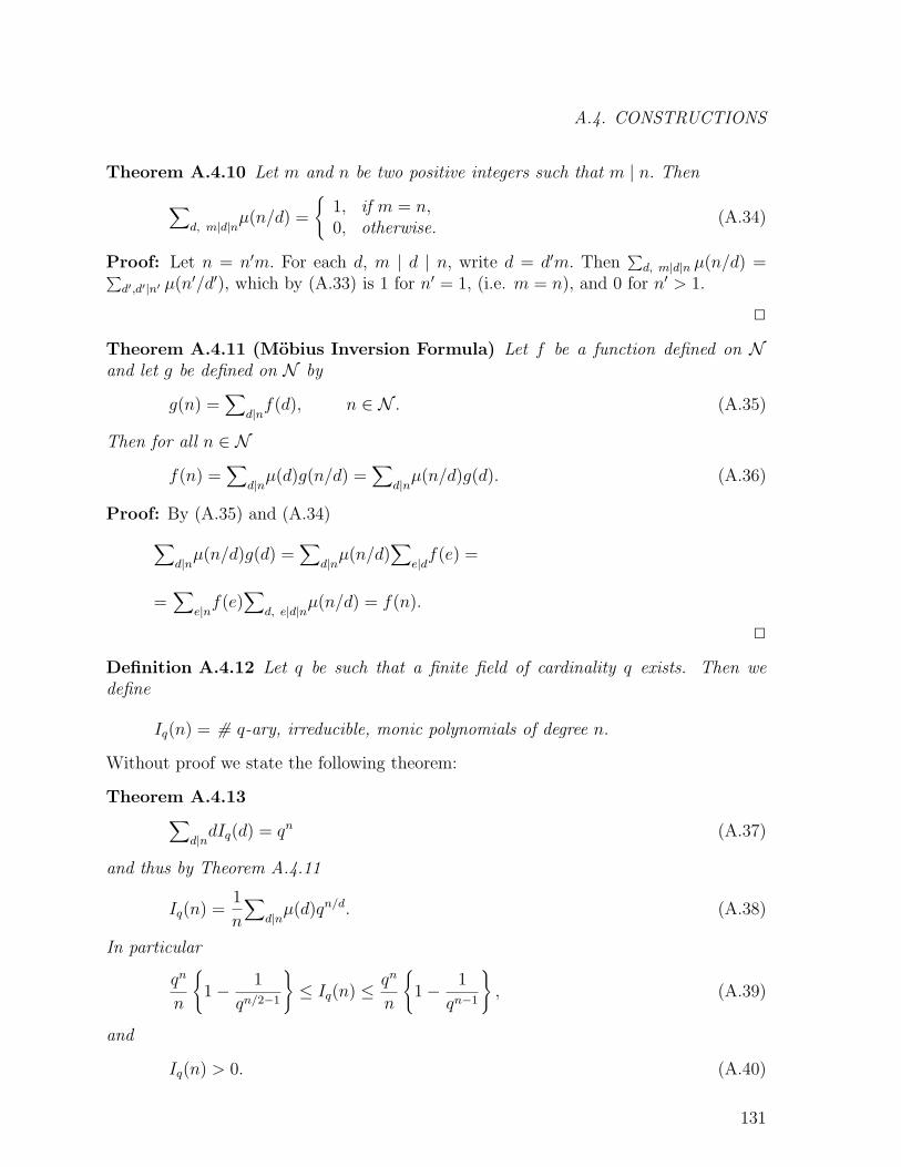
A.4. CONSTRUCTIONS
Theorem A.4.10 Let m and n be two positive integers such that m | n. Then
∑d, m|d|n
µ(n/d) =
{1, if m = n,0, otherwise.
(A.34)
Proof: Let n = n′m. For each d, m | d | n, write d = d′m. Then∑
d, m|d|n µ(n/d) =∑d′,d′|n′ µ(n′/d′), which by (A.33) is 1 for n′ = 1, (i.e. m = n), and 0 for n′ > 1.
2
Theorem A.4.11 (Mobius Inversion Formula) Let f be a function defined on Nand let g be defined on N by
g(n) =∑
d|nf(d), n ∈ N . (A.35)
Then for all n ∈ N
f(n) =∑
d|nµ(d)g(n/d) =
∑d|nµ(n/d)g(d). (A.36)
Proof: By (A.35) and (A.34)∑d|nµ(n/d)g(d) =
∑d|nµ(n/d)
∑e|df(e) =
=∑
e|nf(e)
∑d, e|d|n
µ(n/d) = f(n).
2
Definition A.4.12 Let q be such that a finite field of cardinality q exists. Then wedefine
Iq(n) = # q-ary, irreducible, monic polynomials of degree n.
Without proof we state the following theorem:
Theorem A.4.13∑d|ndIq(d) = qn (A.37)
and thus by Theorem A.4.11
Iq(n) =1
n
∑d|nµ(d)qn/d. (A.38)
In particular
qn
n
{1− 1
qn/2−1
}≤ Iq(n) ≤ qn
n
{1− 1
qn−1
}, (A.39)
and
Iq(n) > 0. (A.40)
131
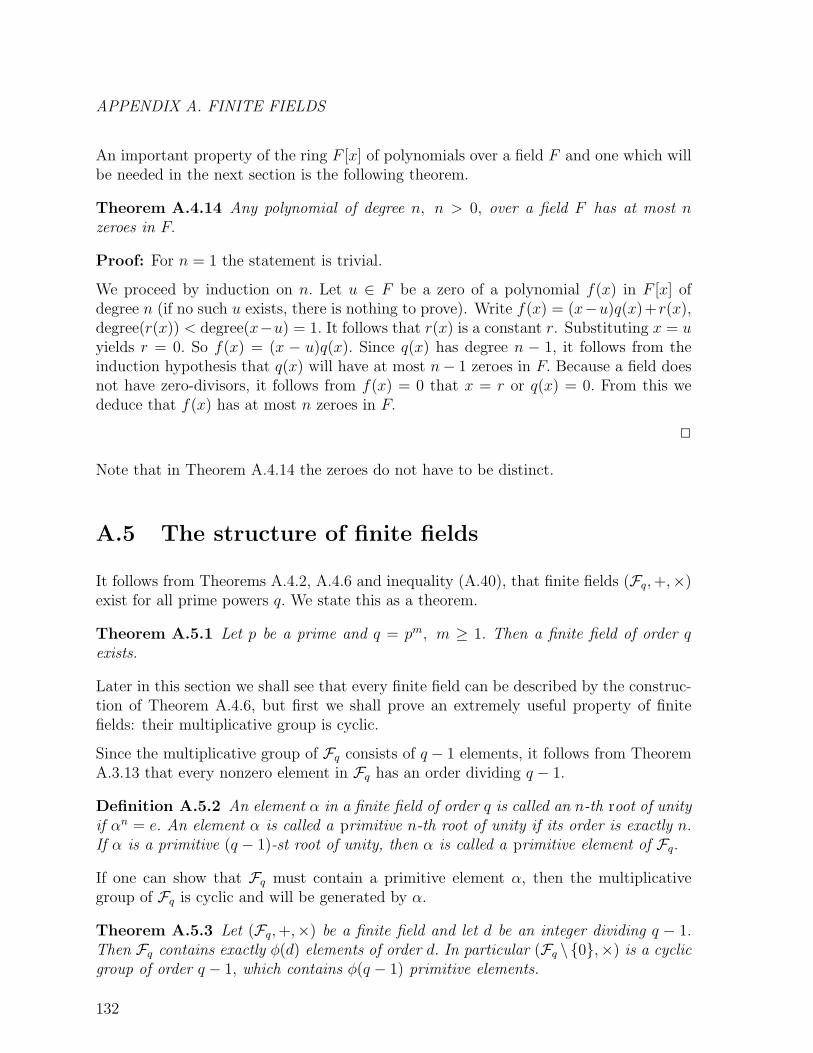
APPENDIX A. FINITE FIELDS
An important property of the ring F [x] of polynomials over a field F and one which willbe needed in the next section is the following theorem.
Theorem A.4.14 Any polynomial of degree n, n > 0, over a field F has at most nzeroes in F.
Proof: For n = 1 the statement is trivial.
We proceed by induction on n. Let u ∈ F be a zero of a polynomial f(x) in F [x] ofdegree n (if no such u exists, there is nothing to prove). Write f(x) = (x−u)q(x)+r(x),degree(r(x)) < degree(x−u) = 1. It follows that r(x) is a constant r. Substituting x = uyields r = 0. So f(x) = (x − u)q(x). Since q(x) has degree n − 1, it follows from theinduction hypothesis that q(x) will have at most n− 1 zeroes in F. Because a field doesnot have zero-divisors, it follows from f(x) = 0 that x = r or q(x) = 0. From this wededuce that f(x) has at most n zeroes in F.
2
Note that in Theorem A.4.14 the zeroes do not have to be distinct.
A.5 The structure of finite fields
It follows from Theorems A.4.2, A.4.6 and inequality (A.40), that finite fields (Fq,+,×)exist for all prime powers q. We state this as a theorem.
Theorem A.5.1 Let p be a prime and q = pm, m ≥ 1. Then a finite field of order qexists.
Later in this section we shall see that every finite field can be described by the construc-tion of Theorem A.4.6, but first we shall prove an extremely useful property of finitefields: their multiplicative group is cyclic.
Since the multiplicative group of Fq consists of q − 1 elements, it follows from TheoremA.3.13 that every nonzero element in Fq has an order dividing q − 1.
Definition A.5.2 An element α in a finite field of order q is called an n-th root of unityif αn = e. An element α is called a primitive n-th root of unity if its order is exactly n.If α is a primitive (q − 1)-st root of unity, then α is called a primitive element of Fq.
If one can show that Fq must contain a primitive element α, then the multiplicativegroup of Fq is cyclic and will be generated by α.
Theorem A.5.3 Let (Fq,+,×) be a finite field and let d be an integer dividing q − 1.Then Fq contains exactly φ(d) elements of order d. In particular (Fq \{0},×) is a cyclicgroup of order q − 1, which contains φ(q − 1) primitive elements.
132
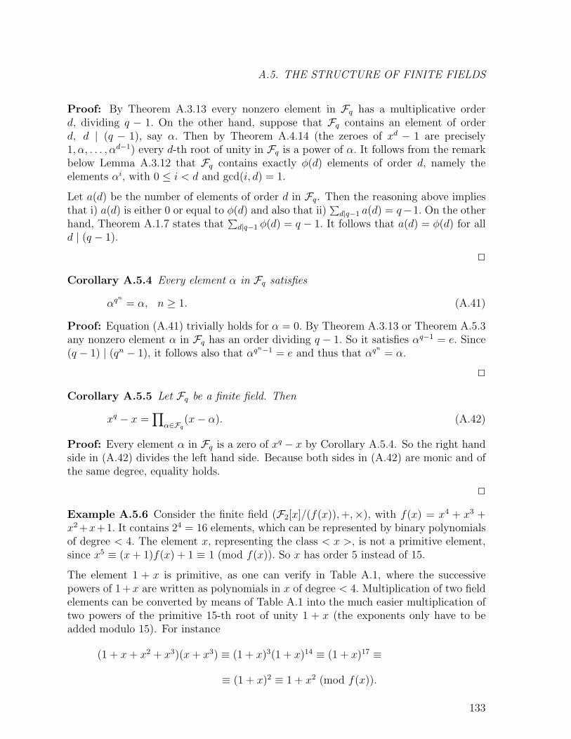
A.5. THE STRUCTURE OF FINITE FIELDS
Proof: By Theorem A.3.13 every nonzero element in Fq has a multiplicative orderd, dividing q − 1. On the other hand, suppose that Fq contains an element of orderd, d | (q − 1), say α. Then by Theorem A.4.14 (the zeroes of xd − 1 are precisely1, α, . . . , αd−1) every d-th root of unity in Fq is a power of α. It follows from the remarkbelow Lemma A.3.12 that Fq contains exactly φ(d) elements of order d, namely theelements αi, with 0 ≤ i < d and gcd(i, d) = 1.
Let a(d) be the number of elements of order d in Fq. Then the reasoning above impliesthat i) a(d) is either 0 or equal to φ(d) and also that ii)
∑d|q−1 a(d) = q−1. On the other
hand, Theorem A.1.7 states that∑
d|q−1 φ(d) = q − 1. It follows that a(d) = φ(d) for alld | (q − 1).
2
Corollary A.5.4 Every element α in Fq satisfies
αqn
= α, n ≥ 1. (A.41)
Proof: Equation (A.41) trivially holds for α = 0. By Theorem A.3.13 or Theorem A.5.3any nonzero element α in Fq has an order dividing q − 1. So it satisfies αq−1 = e. Since(q − 1) | (qn − 1), it follows also that αqn−1 = e and thus that αqn
= α.
2
Corollary A.5.5 Let Fq be a finite field. Then
xq − x =∏
α∈Fq(x− α). (A.42)
Proof: Every element α in Fq is a zero of xq − x by Corollary A.5.4. So the right handside in (A.42) divides the left hand side. Because both sides in (A.42) are monic and ofthe same degree, equality holds.
2
Example A.5.6 Consider the finite field (F2[x]/(f(x)),+,×), with f(x) = x4 + x3 +x2 +x+1. It contains 24 = 16 elements, which can be represented by binary polynomialsof degree < 4. The element x, representing the class < x >, is not a primitive element,since x5 ≡ (x+ 1)f(x) + 1 ≡ 1 (mod f(x)). So x has order 5 instead of 15.
The element 1 + x is primitive, as one can verify in Table A.1, where the successivepowers of 1+x are written as polynomials in x of degree < 4. Multiplication of two fieldelements can be converted by means of Table A.1 into the much easier multiplication oftwo powers of the primitive 15-th root of unity 1 + x (the exponents only have to beadded modulo 15). For instance
(1 + x+ x2 + x3)(x+ x3) ≡ (1 + x)3(1 + x)14 ≡ (1 + x)17 ≡
≡ (1 + x)2 ≡ 1 + x2 (mod f(x)).
133
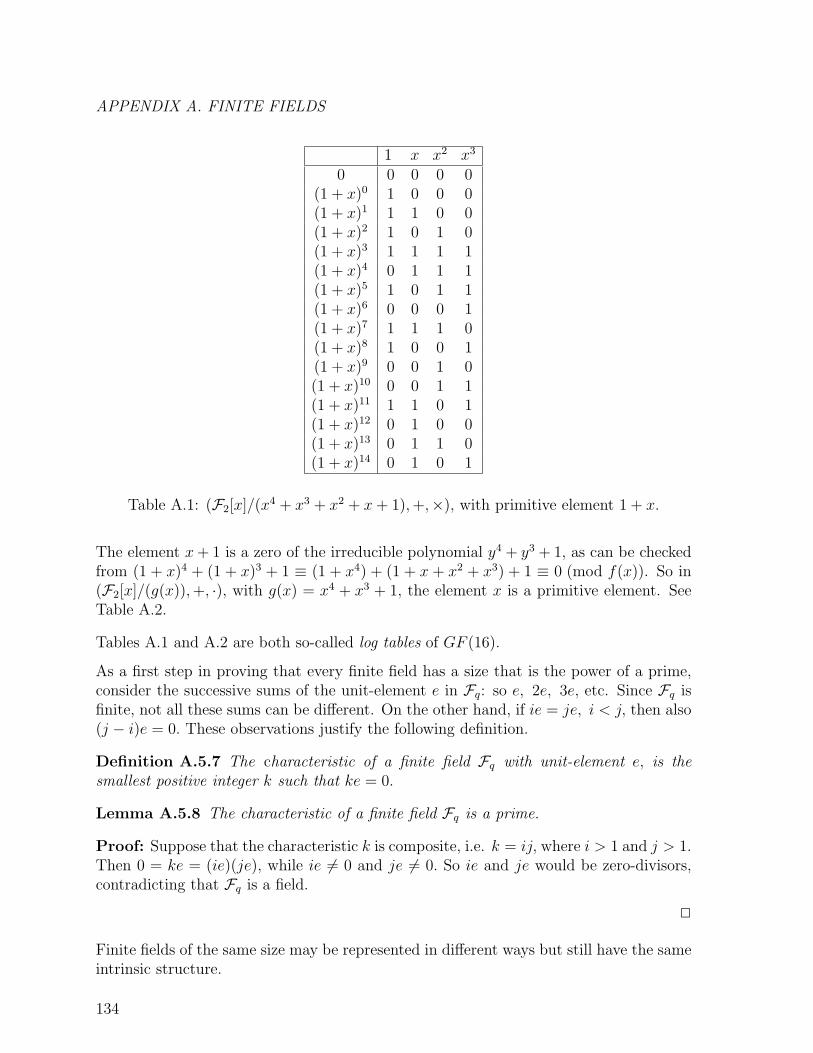
APPENDIX A. FINITE FIELDS
1 x x2 x3
0 0 0 0 0(1 + x)0 1 0 0 0(1 + x)1 1 1 0 0(1 + x)2 1 0 1 0(1 + x)3 1 1 1 1(1 + x)4 0 1 1 1(1 + x)5 1 0 1 1(1 + x)6 0 0 0 1(1 + x)7 1 1 1 0(1 + x)8 1 0 0 1(1 + x)9 0 0 1 0(1 + x)10 0 0 1 1(1 + x)11 1 1 0 1(1 + x)12 0 1 0 0(1 + x)13 0 1 1 0(1 + x)14 0 1 0 1
Table A.1: (F2[x]/(x4 + x3 + x2 + x+ 1),+,×), with primitive element 1 + x.
The element x+ 1 is a zero of the irreducible polynomial y4 + y3 + 1, as can be checkedfrom (1 + x)4 + (1 + x)3 + 1 ≡ (1 + x4) + (1 + x + x2 + x3) + 1 ≡ 0 (mod f(x)). So in(F2[x]/(g(x)),+, ·), with g(x) = x4 + x3 + 1, the element x is a primitive element. SeeTable A.2.
Tables A.1 and A.2 are both so-called log tables of GF (16).
As a first step in proving that every finite field has a size that is the power of a prime,consider the successive sums of the unit-element e in Fq: so e, 2e, 3e, etc. Since Fq isfinite, not all these sums can be different. On the other hand, if ie = je, i < j, then also(j − i)e = 0. These observations justify the following definition.
Definition A.5.7 The characteristic of a finite field Fq with unit-element e, is thesmallest positive integer k such that ke = 0.
Lemma A.5.8 The characteristic of a finite field Fq is a prime.
Proof: Suppose that the characteristic k is composite, i.e. k = ij, where i > 1 and j > 1.Then 0 = ke = (ie)(je), while ie 6= 0 and je 6= 0. So ie and je would be zero-divisors,contradicting that Fq is a field.
2
Finite fields of the same size may be represented in different ways but still have the sameintrinsic structure.
134
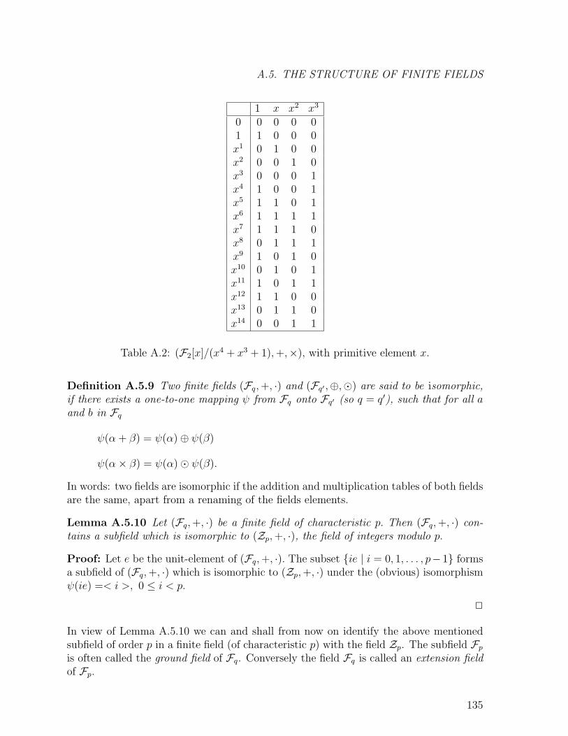
A.5. THE STRUCTURE OF FINITE FIELDS
1 x x2 x3
0 0 0 0 01 1 0 0 0x1 0 1 0 0x2 0 0 1 0x3 0 0 0 1x4 1 0 0 1x5 1 1 0 1x6 1 1 1 1x7 1 1 1 0x8 0 1 1 1x9 1 0 1 0x10 0 1 0 1x11 1 0 1 1x12 1 1 0 0x13 0 1 1 0x14 0 0 1 1
Table A.2: (F2[x]/(x4 + x3 + 1),+,×), with primitive element x.
Definition A.5.9 Two finite fields (Fq,+, ·) and (Fq′ ,⊕,�) are said to be isomorphic,if there exists a one-to-one mapping ψ from Fq onto Fq′ (so q = q′), such that for all aand b in Fq
ψ(α+ β) = ψ(α)⊕ ψ(β)
ψ(α× β) = ψ(α)� ψ(β).
In words: two fields are isomorphic if the addition and multiplication tables of both fieldsare the same, apart from a renaming of the fields elements.
Lemma A.5.10 Let (Fq,+, ·) be a finite field of characteristic p. Then (Fq,+, ·) con-tains a subfield which is isomorphic to (Zp,+, ·), the field of integers modulo p.
Proof: Let e be the unit-element of (Fq,+, ·). The subset {ie | i = 0, 1, . . . , p−1} formsa subfield of (Fq,+, ·) which is isomorphic to (Zp,+, ·) under the (obvious) isomorphismψ(ie) =< i >, 0 ≤ i < p.
2
In view of Lemma A.5.10 we can and shall from now on identify the above mentionedsubfield of order p in a finite field (of characteristic p) with the field Zp. The subfield Fp
is often called the ground field of Fq. Conversely the field Fq is called an extension fieldof Fp.
135

APPENDIX A. FINITE FIELDS
Theorem A.5.11 Let Fq be a finite field of characteristic p. Then q = pm, for someinteger m, m ≥ 1.
Proof: Let m be the size of the smallest basis of Fq over Fp, i.e. m is the smallestinteger such that for suitably chosen elements αi, 1 ≤ i ≤ m, in Fq every element x inFq can be written as
x = u1α1 + u2α2 + · · ·+ umαm,
where ui ∈ Fp, 1 ≤ i ≤ m.
Clearly q ≤ pm. On the other hand it follows from the minimality of m that differentm-tuples u1, u2, . . . , um yield different field elements x. So pm ≥ q. We conclude thatq = pm.
2
At this moment we know that a finite field Fq can only exist for prime powers q. TheoremA.5.1 states that Fq indeed does exist if q is a prime power. That all finite fields of thesame size are in fact isomorphic to each other (and thus can be constructed by TheoremA.4.6) will be proved later.
Theorem A.5.12 Let α be an element in a finite field Fq of characteristic p. Then overFp (and any extension field of it)
(x− α)p = xp − αp. (A.43)
Proof: Let 0 < i < p. Then gcd(p, i!) = 1, so(pi
)≡ p(p−1)···(p−i+1)
i(i−1)···2·1 ≡ p (p−1)···(p−i+1)i(i−1)···2·1 ≡ 0 (mod p).
And so with the binomial theorem, we have that
(x− α)p = xp + (−α)p = xp − αp,
where the last equality is obvious for odd p, while for p = 2 this equality follows from+1 = −1.
2
Corollary A.5.13 Let αi, 1 ≤ i ≤ k, be elements in a finite field Fq of characteristicp. Then for every n
(∑k
i=1αi
)pn
=∑k
i=1αpn
i .
Proof: For k = 2, n = 1 the statement follows again from the previous theorem (takex = −α1, α = α2). Next use an induction argument on k and finally on n.
136
A.5. THE STRUCTURE OF FINITE FIELDS
2
The following theorem often gives a powerful criterion to determine whether an elementin a field Fq of characteristic p, actually lies in its ground field Fp.
Theorem A.5.14 Let Fq be a finite field of characteristic p. So q = pm, m > 0, andFq contains Fp as a subfield. Let α be an element in Fq. Then α is an element of thesubfield Fp if and only if α satisfies
αp = α. (A.44)
Proof: The p elements in the subfield Fp satisfy (A.44) by Corollary A.5.4. On theother hand the polynomial xp − x has at most p zeroes in Fq by Theorem A.4.14, so itcan not have any other zeroes.
2
Let α be an element in Fq, a field of characteristic p, but α 6∈ Fp. Then αp 6= α by theprevious theorem. Still there is a relation between αp and α.
Theorem A.5.15 Let α be an element in a finite field Fq of characteristic p. Let f(x)be a polynomial over Fp such that f(α) = 0. Then for all n ∈ N
f(αpn
) = 0. (A.45)
Proof: Write f(x) =∑m
i=0 fixi, fi ∈ Fp. By Theorem A.5.14, fpn
i = fi, 0 ≤ i ≤ m. Henceby Corollary A.5.13
0 = (f(α))pn= (
∑m
i=0fiα
i)pn=∑m
i=0(fiα
i)pn=
∑m
i=0fpn
i αi·pn=∑m
i=0fi(α
pn)i = f(αpn
).
2
In the field R and its extension field C a similar phenomenon occurs. If f(x) is apolynomial over the reals and f(a) = 0, a ∈ C , then also f(a) = 0, where a is thecomplex conjugate of a.
The following theorem states that the number of different elements αpn, n = 0, 1, . . . ,
only depends on the numbers p and the order of α. Note that an element in a finite fieldof characteristic p will have an order dividing pm − 1 for some value of m and thus thisorder will have no factor in common with p.
Theorem A.5.16 Let α be an element of order n in a finite field of characteristic p. Letm be the multiplicative order of p modulo n, i.e. pm ≡ 1 (mod n), with m ≥ 1 minimal.Then the m elements
α, αp, αp2, . . . , αpm−1
137
APPENDIX A. FINITE FIELDS
are all distinct and αpm= α.
Proof: By Lemma A.3.11 (twice) one has that αpi= αpj
if and only if pi ≡ pj (mod n),i.e. iff pi−j ≡ 1 (mod n), i.e. iff i ≡ j (mod m).
2
The m elements α, αp, αp2, . . . , αpm−1
in Theorem A.5.16 are called the conjugates of α.
Example A.5.17 Consider (F2[x]/(f(x)),+, ·) with f(x) = x4 + x3 + x2 + x + 1 (seeExample A.5.6). The element x has order 5. The multiplicative order of 2 modulo 5 is4. So x, x2, x22
and x23are all different, while x24
= x. Indeed, x8 ≡ x3 (mod f(x)) andx16 ≡ x (mod f(x)).
Theorem A.5.18 Let α be an element of order n in a finite field Fq of characteristicp. Let m be the multiplicative order of p modulo n. Then the q-ary polynomial
m(x) =∏m−1
i=0(x− αpi
) (A.46)
is in fact a polynomial with coefficients in Fp, moreover m(x) is irreducible over Fp.
Proof: Clearly m(x) is a polynomial over Fq. Write m(x) =∑m
i=0mix
i. Then by Theo-rems A.5.12 and A.5.16
(m(x))p =∏m−1
i=0(x− αpi
)p =∏m−1
i=0(xp − αpi+1
) =
=∏m
i=1(xp − αpi
) =∏m−1
i=0(xp − αpi
) = m(xp).
Hence∑m
i=0mix
pi = m(xp) = (m(x))p =(∑m
i=0mix
i)p
=∑m
i=0mp
ixpi.
Comparing the coefficients of xpi on both hands yields mi = mpi . From Theorem A.5.14
we conclude that mi ∈ Fp, 0 ≤ i ≤ m. So m(x) is a polynomial in Fp[x]. From TheoremsA.5.15 and A.5.16 it follows that no polynomial in Fp[x] of degree less than m can haveα as a zero. So m(x) is irreducible in Fp[x].
2
Corollary A.5.19 Let α be an element of order n in a finite field of characteristic p.Let m(x) be defined by (A.46) and let f(x) be any p-ary polynomial that has α as zero.Then f(x) is a multiple of m(x).
Proof: Combine Theorems A.5.15, A.5.16 and A.5.18.
2
So m(x) is the monic polynomial of lowest degree over Fp, having α as a zero. For thisreason the polynomial m(x) is called the minimal polynomial of α. It has α and all the
138
A.5. THE STRUCTURE OF FINITE FIELDS
conjugates of α as zeroes. The degree of the minimal polynomial m(x) of an element αis often simply called the degree of α.
If m(x) is the minimal polynomial of a primitive element, then m(x) is called a prim-itive polynomial. Let α be a zero of a primitive polynomial m(x). Often the minimalpolynomial of a power αi will be denoted by mi(x).
Example A.5.20 Consider (F2[x]/(f(x)),+, ·) with f(x) a fourth degree irreduciblepolynomial and let α be one of the primitive elements of this field.
Clearly m0(x) = x − 1. Also m3(x) and m5(x) are easily determined. Indeed, m5(x)has as zeroes α5 and its conjugates, so α5 and α10. Both these elements have order 3,and thus they are both zeroes of (x3 − 1)/(x − 1) = x2 + x + 1. We conclude thatm5(x) = x2 + x + 1. For exactly the same reason the four primitive 5-th roots of unityα3, α6, α9, α12 form the zeroes of m3(x) = x4 + x3 + x2 + x+ 1.
Since there are only two irreducible polynomials of degree four left, being x4 +x+1 andx4 + x3 + 1, it follows that m1(x) = x4 + x + 1 and m−1(x) = m7(x) = x4 + x3 + 1, orthe other way around. Both apparently are primitive polynomials.
Let m(x) be the minimal polynomial of an element α of degree m. It follows fromCorollary A.5.19 that the pm expressions
∑m−1i=0 fiα
i, fi ∈ Fp, 0 ≤ i < m, take on pm
different values. For these expressions addition and multiplication can be performed,just as in (A.30) and (A.31), where now m(α) = 0 has to be used to reduce the degreeof the outcome to a value less than m. It is quite easy to check that one obtains a field,that is isomorphic to Fp[x]/(m(x)) and that clearly contains α.
If m(x) is primitive, one has that 1, x, . . . , xpm−2 are all different modulo m(x), just asthe elements 1, α, . . . , αpm−2 are all different. See for instance Example A.5.6, where theprimitive element a = 1+x has minimal polynomial m(y) = 1+y3 +y4. Table A.2 showsthe field F2[y]/(m(y)).
Lemma A.5.21 Let m(x) be an irreducible polynomial of degree m over a field with pelements and let n be a multiple of m. Then m(x) divides xpn − x.
Proof: Consider the residue class ring Fp[x]/(m(x)). This ring is a field with q = pm
elements by Theorem A.4.6. The field element α =< x > is a zero of m(x), sincem(α) = m(< x >) =< m(x) >=< 0 > . It follows from Corollary A.5.4 that α =< x >is a zero of xpn − x, n ≥ 1. By Corollary A.5.19 m(x) divides xpn − x.
2
Also the converse of Lemma A.5.21 is true.
Theorem A.5.22 Over Fp[x] the polynomial xpn − x is the product of all irreducible,monic, p-ary polynomials with a degree dividing n.
Proof: Let m | n. By definition, there are Ip(m) irreducible p-ary polynomials of degreem, all of which divide xpn − x by Lemma A.5.21. The sum of their degrees is mIp(m).
139
APPENDIX A. FINITE FIELDS
But∑
m|nmIp(m) = pn by (A.37), which is the degree of (xpn − x). It follows thatthe product of all irreducible, monic, p-ary polynomials of degree m, m | n, forms thecomplete factorization of xpn − x.
2
Example A.5.23 p = 2, n = 4, I2(1) = 2, I2(2) = 1 and I2(4) = 3 (see Section A.4).As follows from Theorem A.5.22, but can also be checked directly, one indeed has that
x16 − x =
= x(x+ 1)(x2 + x+ 1)(x4 + x+ 1)(x4 + x3 + 1)(x4 + x3 + x2 + x+ 1).
Corollary A.5.24 Let f(x) be an irreducible polynomial in Fp[x] of degree m. Let m | n.Then a finite field with pn elements contains m roots of f(x).
Proof: By Theorem A.5.22 f(x) divides xq − x, q = pn. On the other hand xq − x =∏α∈Fq
(x− α), by (A.42).
2
Theorem A.5.25 Let p be a prime and m in N . Then the finite field Fpm is unique,up to isomorphism.
Proof: Write q = pm and let Fq be any finite field of order q. Let f(x) be any irreducible,p-ary polynomial of degree m. We shall show that Fq is isomorphic to Fp[x]/(f(x)).
By Corollary A.5.24 Fq contains m zeroes of f(x). Let α be one of these m zeroes. Sincef(x) is irreducible in Fp[x], we know that 1, α, . . . , αm−1 are independent over Fp. Soany element in Fq can be uniquely written as
∑m−1i=0 uiα
i, ui ∈ Fp, 0 ≤ i ≤ m− 1.
The isomorphism Fq between and Fp[x]/(f(x)) is given by ψ(∑m−1
i=0 uiαi) =
∑m−1i=0 uix
i.
2
Corollary A.5.26 Fpm is (isomorphic to) a subfield of Fpn if and only if m divides n.
Proof: The following assertions are all equivalent:
i) m | n,ii) (pm − 1) | (pn − 1),
iii) xpm − x divides xpn − x,iv)
∏α∈Fpm (x− α) divides
∏α∈Fpn (x− α),
v) Fpm is (isomorphic to) a subfield of Fpn . 2
Example A.5.27 It follows from Corollary A.5.26 that F24 contains F22 as a subfield,but does not contain F23 as a subfield. From Table A.2 one can easily verify that theelements 0, 1, x5 and x10 form the subfield of order 22 in F2[x]/(x
4 + x3 + 1).
140
A.6. PROBLEMS
Most of the time in this appendix we have viewed Fq, q = pm and p prime, as an extensionfield of Fp. But all the concepts, defined in this appendix, can also be generalized toFq[x]. So one may want to count the number of irreducible polynomials of degree n inFq[x] or discuss primitive polynomials over Fq, etc. We leave it to the reader to verifythat all the theorems in this appendix can indeed be generalized from Fp and Fpm to Fq
resp. Fqm , simply by replacing p by q and q by qm.
Example A.5.28 The field F16 can be viewed as the residue class ring F4[x]/ (x2 +x+α), where α is an element in F4, satisfying α2 + α+ 1 = 0.
A.6 Problems
A.6.1 Let the sequence of Fibonacci numbers {Fn}∞n=0 be defined recursively by F0 = 0,F1 = 1 and Fn = Fn−1 + Fn−2, n ≥ 2.
Show that for n ≥ 3 Euclid’s Algorithm (Algorithm A.1.3) applied to Fn−1 and Fn
determines their gcd in exactly n− 2 iterations.
A.6.2 Use an induction argument to show that the computation of the gcd of integersa and b, b ≥ a, by Euclid’s Algorithm involves at most b logf bc iterations, where
f = (1 +√
5)/2. (Hint: distinguish the cases a ≤ b/f and b/f < a ≤ b.)
Note that b logf Fnc = n− 2.
A.6.3 Let p be a prime number dividing a1a2 · · · ak, where ai ∈ Z, 1 ≤ i ≤ k. Show thatp divides at least one of the factors ai, 1 ≤ i ≤ k.
Prove Theorem A.1.5.
A.6.4 Describe the congruence relation, as defined in (A.16), as an equivalence relation(see Definition A.2.1), so give the sets S and U.
A.6.5 Give a formal proof of Lemma A.3.5.
A.6.6 Prove the equivalence of (H2) and (H3) with (H) in Section A.3.
A.6.7 What are the subgroups of (Z15,+) and of (Z∗17,×) ?
What is the multiplicative order of the various elements in (Z∗17,×)?
A.6.8 Prove that (A.25) indeed defines an equivalence relation and show that the equiv-alence classes are given by {ha | h ∈ H}, where a ∈ G.
A.6.9 Prove that the set (1 + x3) in F2[x], consisting of all polynomial multiples of thepolynomial 1 + x3, is an ideal in (F2[x],+,×).
Give a pair of zero-divisors in the residue class ring (F2[x]/(1 + x3),+,×).
141

APPENDIX A. FINITE FIELDS
A.6.10 What is the product of the binary polynomials 1+x2 +x4 and 1+x+x3 modulo1 + x2 + x5?
A.6.11 Find all binary, irreducible polynomials of degree 2, 3, and 4 and check (A.38).
A.6.12 Use Euclid’s Algorithm to find the multiplicative inverse of 1 + x+ x3 (mod 1 +x2 + x5) over F2.
A.6.13 What are the multiplicative orders of x and of x2 +x3 in (F2[x]/(1+x+x2 +x3 +x4),+,×)? What is the product of these two elements and what is its multiplicativeorder?
A.6.14 Make a log table of GF (3)[x]/(2 + 2x+ x2) (hint: x is a primitive element).
A.6.15 Let α be a primitive element of GF (26). Determine the zeroes of the minimalpolynomials of α, α3 and α9.
A.6.16 What is the smallest extension field of GF (3) containing a primitive 11-th rootof unity α?
What is the degree of the minimal polynomial of α and what are the zeroes of thispolynomial?
A.6.17 Which subfields are contained in GF (625). Let α be a primitive element inGF (625). Which powers of α constitute the various subfields of GF (625).
A.6.18 What is the degree of a binary minimal polynomial of a primitive 17-th root ofunity? How many such polynomials do exist? Prove that each is its own reciprocal.Determine them explicitly.
A.6.19 The trace mapping Tr is defined on GF (pm), p prime, by
Tr(x) = x+ xp + xp2+ · · ·+ xpm−1
.
1. Prove that Tr(x) ∈ GF (p), for every x ∈ GF (pm). So Tr is a mapping fromGF (pm) to GF (p).
2. Prove that Tr is a linear mapping from GF (pm) to GF (p).
3. Prove that Tr takes on every value in GF (p) equally often (hint: use TheoremA.4.14).
142
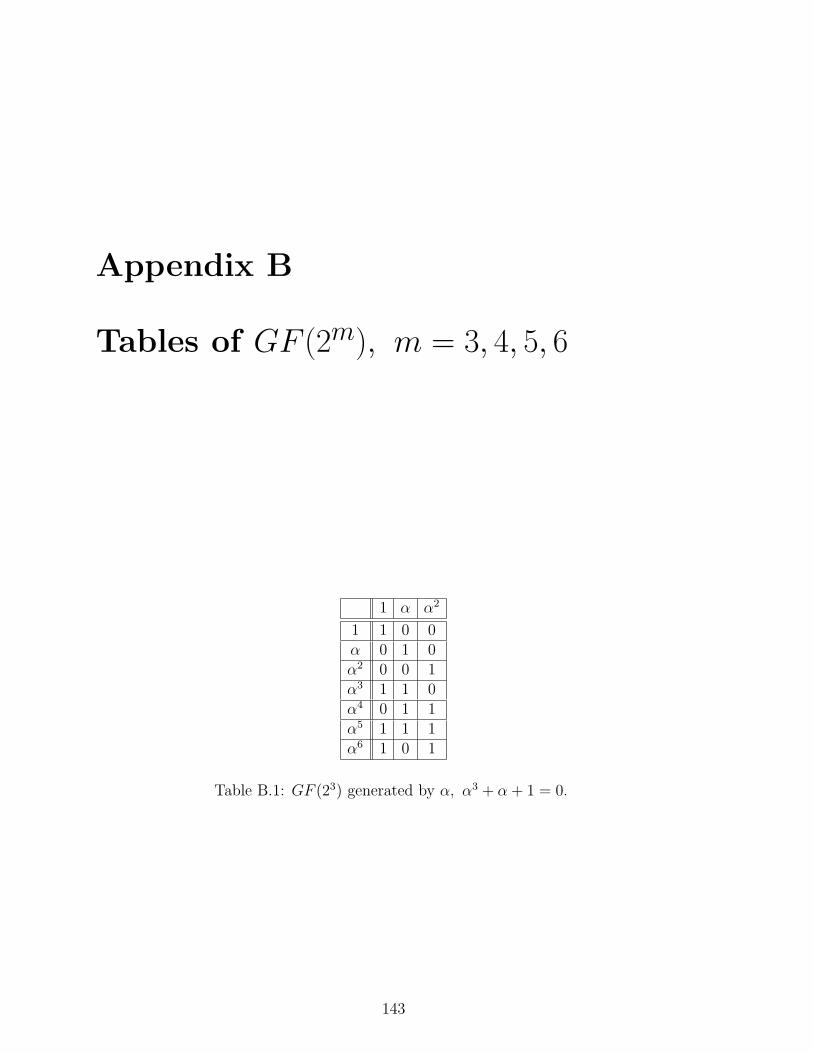
Appendix B
Tables of GF (2m), m = 3, 4, 5, 6
1 α α2
1 1 0 0α 0 1 0α2 0 0 1α3 1 1 0α4 0 1 1α5 1 1 1α6 1 0 1
Table B.1: GF (23) generated by α, α3 + α+ 1 = 0.
143
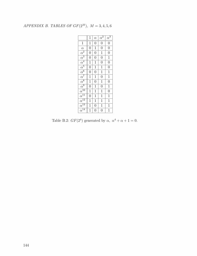
APPENDIX B. TABLES OF GF (2M), M = 3, 4, 5, 6
1 α α2 α3
1 1 0 0 0α 0 1 0 0α2 0 0 1 0α3 0 0 0 1α4 1 1 0 0α5 0 1 1 0α6 0 0 1 1α7 1 1 0 1α8 1 0 1 0α9 0 1 0 1α10 1 1 1 0α11 0 1 1 1α12 1 1 1 1α13 1 0 1 1α14 1 0 0 1
Table B.2: GF (24) generated by α, α4 + α+ 1 = 0.
144
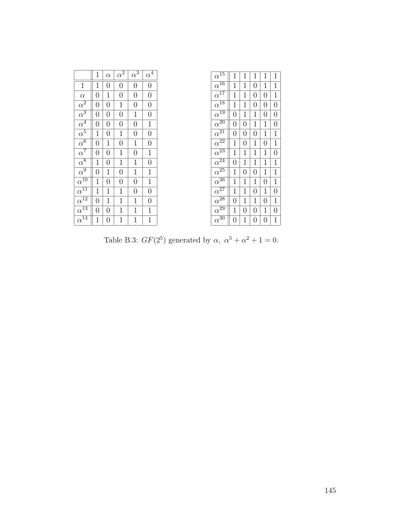
1 α α2 α3 α4
1 1 0 0 0 0α 0 1 0 0 0α2 0 0 1 0 0α3 0 0 0 1 0α4 0 0 0 0 1α5 1 0 1 0 0α6 0 1 0 1 0α7 0 0 1 0 1α8 1 0 1 1 0α9 0 1 0 1 1α10 1 0 0 0 1α11 1 1 1 0 0α12 0 1 1 1 0α13 0 0 1 1 1α14 1 0 1 1 1
α15 1 1 1 1 1α16 1 1 0 1 1α17 1 1 0 0 1α18 1 1 0 0 0α19 0 1 1 0 0α20 0 0 1 1 0α21 0 0 0 1 1α22 1 0 1 0 1α23 1 1 1 1 0α24 0 1 1 1 1α25 1 0 0 1 1α26 1 1 1 0 1α27 1 1 0 1 0α28 0 1 1 0 1α29 1 0 0 1 0α30 0 1 0 0 1
Table B.3: GF (25) generated by α, α5 + α2 + 1 = 0.
145
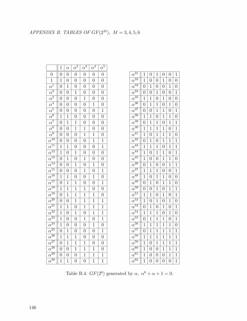
APPENDIX B. TABLES OF GF (2M), M = 3, 4, 5, 6
1 α α2 α3 α4 α5
0 0 0 0 0 0 01 1 0 0 0 0 0α1 0 1 0 0 0 0α2 0 0 1 0 0 0α3 0 0 0 1 0 0α4 0 0 0 0 1 0α5 0 0 0 0 0 1α6 1 1 0 0 0 0α7 0 1 1 0 0 0α8 0 0 1 1 0 0α9 0 0 0 1 1 0α10 0 0 0 0 1 1α11 1 1 0 0 0 1α12 1 0 1 0 0 0α13 0 1 0 1 0 0α14 0 0 1 0 1 0α15 0 0 0 1 0 1α16 1 1 0 0 1 0α17 0 1 1 0 0 1α18 1 1 1 1 0 0α19 0 1 1 1 1 0α20 0 0 1 1 1 1α21 1 1 0 1 1 1α22 1 0 1 0 1 1α23 1 0 0 1 0 1α24 1 0 0 0 1 0α25 0 1 0 0 0 1α26 1 1 1 0 0 0α27 0 1 1 1 0 0α28 0 0 1 1 1 0α29 0 0 0 1 1 1α30 1 1 0 0 1 1
α31 1 0 1 0 0 1α32 1 0 0 1 0 0α33 0 1 0 0 1 0α34 0 0 1 0 0 1α35 1 1 0 1 0 0α36 0 1 1 0 1 0α37 0 0 1 1 0 1α38 1 1 0 1 1 0α39 0 1 1 0 1 1α40 1 1 1 1 0 1α41 1 0 1 1 1 0α42 0 1 0 1 1 1α43 1 1 1 0 1 1α44 1 0 1 1 0 1α45 1 0 0 1 1 0α46 0 1 0 0 1 1α47 1 1 1 0 0 1α48 1 0 1 1 0 0α49 0 1 0 1 1 0α50 0 0 1 0 1 1α51 1 1 0 1 0 1α52 1 0 1 0 1 0α53 0 1 0 1 0 1α54 1 1 1 0 1 0α55 0 1 1 1 0 1α56 1 1 1 1 1 0α57 0 1 1 1 1 1α58 1 1 1 1 1 1α59 1 0 1 1 1 1α60 1 0 0 1 1 1α61 1 0 0 0 1 1α62 1 0 0 0 0 1
Table B.4: GF (26) generated by α, α6 + α+ 1 = 0.
146
Appendix C
Solutions to the problems
C.1 Solutions to Chapter 1
1.4.1 When 000000 has been transmitted, the receiver will not detect transmission errorsif the error pattern is 001111, 110011 or 111100. This happens with probablityp4(1− p)2 + p4(1− p)2 + p4(1− p)2.
One finds the same probability of undetected error when one of the other threewords has been transmitted. So the overall probability of undetected error is equalto 3p4(1− p)2.
1.4.2 It follows from
p(−1| − 1)p(0.01| − 1)p(0.01| − 1) =
=(
1√2π
)3e−(02+1.012+1.012)/2
≈ 0.0229.
and
p(−1|+ 1)p(0.01|+ 1)p(0.01|+ 1) =
=(
1√2π
)3e−(22+0.992+0.992)/2
≈ 0.0032.
that any reasonable soft decision decoding rule will decode (−1, 0.01, 0.01) into(−1,−1,−1).
With hard decision decoding the received sequence is transformed into(−1,+1,+1). Now (+1,+1,+1) is the most likely transmitted word, because theprobability that (+1,+1,+1) is transmitted given that (−1,+1,+1) is received isp(1−p)2 with p = 1√
2π
∫x≥0 e
−(x+1)2/2dx. This exceeds the probability that (−1,−1,
−1) is transmitted given that (−1,+1,+1) is received, which is p2(1− p).
147
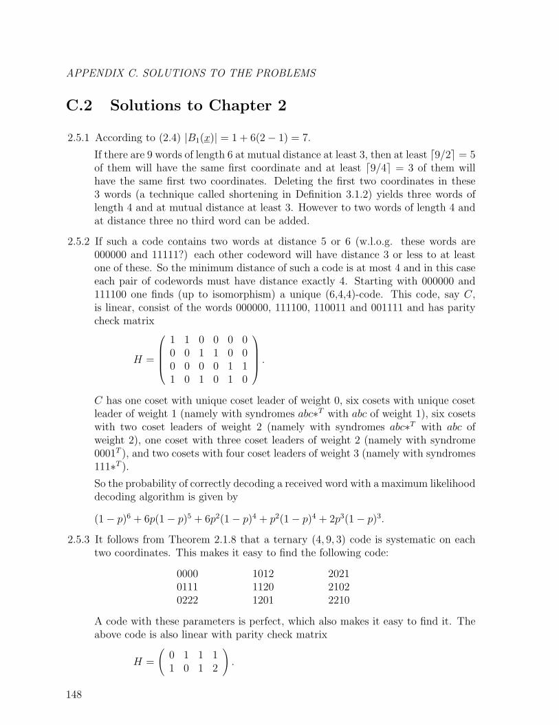
APPENDIX C. SOLUTIONS TO THE PROBLEMS
C.2 Solutions to Chapter 2
2.5.1 According to (2.4) |B1(x)| = 1 + 6(2− 1) = 7.
If there are 9 words of length 6 at mutual distance at least 3, then at least d9/2e = 5of them will have the same first coordinate and at least d9/4e = 3 of them willhave the same first two coordinates. Deleting the first two coordinates in these3 words (a technique called shortening in Definition 3.1.2) yields three words oflength 4 and at mutual distance at least 3. However to two words of length 4 andat distance three no third word can be added.
2.5.2 If such a code contains two words at distance 5 or 6 (w.l.o.g. these words are000000 and 11111?) each other codeword will have distance 3 or less to at leastone of these. So the minimum distance of such a code is at most 4 and in this caseeach pair of codewords must have distance exactly 4. Starting with 000000 and111100 one finds (up to isomorphism) a unique (6,4,4)-code. This code, say C,is linear, consist of the words 000000, 111100, 110011 and 001111 and has paritycheck matrix
H =
1 1 0 0 0 00 0 1 1 0 00 0 0 0 1 11 0 1 0 1 0
.C has one coset with unique coset leader of weight 0, six cosets with unique cosetleader of weight 1 (namely with syndromes abc∗T with abc of weight 1), six cosetswith two coset leaders of weight 2 (namely with syndromes abc∗T with abc ofweight 2), one coset with three coset leaders of weight 2 (namely with syndrome0001T ), and two cosets with four coset leaders of weight 3 (namely with syndromes111∗T ).
So the probability of correctly decoding a received word with a maximum likelihooddecoding algorithm is given by
(1− p)6 + 6p(1− p)5 + 6p2(1− p)4 + p2(1− p)4 + 2p3(1− p)3.
2.5.3 It follows from Theorem 2.1.8 that a ternary (4, 9, 3) code is systematic on eachtwo coordinates. This makes it easy to find the following code:
0000 1012 20210111 1120 21020222 1201 2210
A code with these parameters is perfect, which also makes it easy to find it. Theabove code is also linear with parity check matrix
H =
(0 1 1 11 0 1 2
).
148
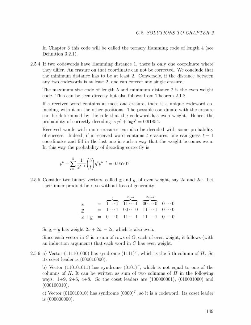
C.2. SOLUTIONS TO CHAPTER 2
In Chapter 3 this code will be called the ternary Hamming code of length 4 (seeDefinition 3.2.1).
2.5.4 If two codewords have Hamming distance 1, there is only one coordinate wherethey differ. An erasure on that coordinate can not be corrected. We conclude thatthe minimum distance has to be at least 2. Conversely, if the distance betweenany two codewords is at least 2, one can correct any single erasure.
The maximum size code of length 5 and minimum distance 2 is the even weightcode. This can be seen directly but also follows from Theorem 2.1.8.
If a received word contains at most one erasure, there is a unique codeword co-inciding with it on the other positions. The possible coordinate with the erasurecan be determined by the rule that the codeword has even weight. Hence, theprobability of correctly decoding is p5 + 5qp4 = 0.91854.
Received words with more erasures can also be decoded with some probabilityof success. Indeed, if a received word contains t erasures, one can guess t − 1coordinates and fill in the last one in such a way that the weight becomes even.In this way the probability of decoding correctly is
p5 +5∑
t=1
1
2t−1
(5
t
)qtp5−t = 0.95707.
2.5.5 Consider two binary vectors, called x and y, of even weight, say 2v and 2w. Lettheir inner product be i, so without loss of generality:
x =
i︷ ︸︸ ︷1 · · · 1
2v−i︷ ︸︸ ︷11 · · · 1
2w−i︷ ︸︸ ︷00 · · · 0 0 · · · 0
y = 1 · · · 1 00 · · · 0 11 · · · 1 0 · · · 0x+ y = 0 · · · 0 11 · · · 1 11 · · · 1 0 · · · 0
So x+ y has weight 2v + 2w − 2i, which is also even.
Since each vector in C is a sum of rows of G, each of even weight, it follows (withan induction argument) that each word in C has even weight.
2.5.6 a) Vector (111101000) has syndrome (1111)T , which is the 5-th column of H. Soits coset leader is (000010000).
b) Vector (110101011) has syndrome (0101)T , which is not equal to one of thecolumns of H. It can be written as sum of two columns of H in the followingways: 1+9, 2+6, 4+8. So the coset leaders are (100000001), (010001000) and(000100010).
c) Vector (010010010) has syndrome (0000)T , so it is a codeword. Its coset leaderis (000000000).
149

APPENDIX C. SOLUTIONS TO THE PROBLEMS
2.5.7 Take two rows from G, say x and y. Use the same approach as in the solution ofProblem 2.5.5. The weights of x and y can now be written as 4v and 4w and theirinner product (x, y) as 2i, because C is self dual and thus each inner product iseven. It follows that x + y has weight 4v + 4w − 2 · 2i, which is again a multipleof four.
For an arbitrary vector in the code, which is the sum of rows of G, one again usesan induction argument.
2.5.8 If all the codewords have a weight divisible by 4, it follows that 1 is in the dualcode C⊥. Since C = C⊥ we can conclude that 1 is an element in C.
Let Ai, 0 ≤ i ≤ 24, be the weight enumerator of C. Since 1 ∈ C it follows thatAi = A24−i From d = 8 and the divisibility of all weights by 4, the non-zerocoefficients in the weight enumerator are A0 = A24 = 1, A8 = A16 and A12. Since|C| = 212 also the relation 2+2A8 +A12 = 4096 holds. We need one more relation.
The coefficient of z2 in the MacWilliams relation (2.22) gives:
0 =
(24
2
)+ A8
((8
2
)− 8
)+ A12(−12) +
+A8
((8
2
)− 8
)+
(24
2
),
i.e.
−10A8 + 3A12 = 138.
Combining the two relations yields the weight enumerator A0 = A24 = 1, A8 =A16 = 759 and A12 = 2576.
2.5.9 A vector c is in the code C if and only if HcT = 0T , i.e. if and only if the columnsin H corresponding to the non-zero coordinates of c are linearly dependent.
A vector x is at distance δ from the code C if it is in a coset with coset leader ofweight δ, i.e. if it (or the coset leader) can be written as linear combination of δcolumns of H but not of less.
2.5.10 Consider a k-tuple of coordinates. Puncturing the other d− 1 coordinates in thecode yields, according to the proof of Theorem 2.1.8, a (k, qk, 1) code. So C issystematic on these k coordinates.
Consider any d-tuple of coordinates, put α 6= 0 on the leftmost of these coordinatesand put zeros on the complementary n−d = k−1 positions. Since C is systematicon these k coordinates, it follows that exactly one codeword exists that coincideswith these k entries. From the minimum distance d one can conclude that this
150
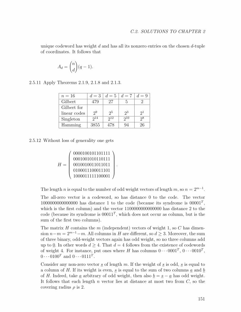
C.2. SOLUTIONS TO CHAPTER 2
unique codeword has weight d and has all its nonzero entries on the chosen d-tupleof coordinates. It follows that
Ad =
(n
d
)(q − 1).
2.5.11 Apply Theorems 2.1.9, 2.1.8 and 2.1.3.
n = 16 d = 3 d = 5 d = 7 d = 9Gilbert 479 27 5 2Gilbert forlinear codes 29 25 23 21
Singleton 214 212 210 28
Hamming 3855 478 94 26
2.5.12 Without loss of generality one gets
H =
00001001011011110001001010110111001001001101101101000111000111011000011111100001
.
The length n is equal to the number of odd weight vectors of lengthm, so n = 2m−1.
The all-zero vector is a codeword, so has distance 0 to the code. The vector1000000000000000 has distance 1 to the code (because its syndrome is 00001T ,which is the first column) and the vector 1100000000000000 has distance 2 to thecode (because its syndrome is 00011T , which does not occur as column, but is thesum of the first two columns).
The matrix H contains the m (independent) vectors of weight 1, so C has dimen-sion n−m = 2m−1−m. All columns in H are different, so d ≥ 3. Moreover, the sumof three binary, odd-weight vectors again has odd weight, so no three columns addup to 0. In other words d ≥ 4. That d = 4 follows from the existence of codewordsof weight 4. For instance, put ones where H has columns 0 · · · 0001T , 0 · · · 0010T ,0 · · · 0100T and 0 · · · 0111T .
Consider any non-zero vector s of length m. If the weight of s is odd, s is equal toa column of H. If its weight is even, s is equal to the sum of two columns a and bof H. Indeed, take a arbitrary of odd weight, then also b = s− a has odd weight.It follows that each length n vector lies at distance at most two from C, so thecovering radius ρ is 2.
151
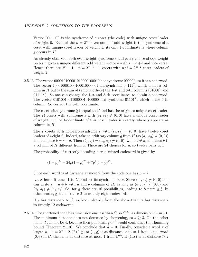
APPENDIX C. SOLUTIONS TO THE PROBLEMS
Vector 00 · · · 0T is the syndrome of a coset (the code) with unique coset leaderof weight 0. Each of the n = 2m−1 vectors s of odd weight is the syndrome of acoset with unique coset leader of weight 1: its only 1-coordinate is where columns occurs in H.
As already observed, each even weight syndrome s and every choice of odd weightvector a gives a unique different odd weight vector b with s = a+ b and vice versa.Hence, there are 2m − 1 − n = 2m−1 − 1 cosets with n/2 = 2m−2 coset leaders ofweight 2.
2.5.13 The vector 000010100001010000100010 has syndrome 00000T , so it is a codeword.The vector 100010001000100010000001 has syndrome 00111T , which is not a col-umn in H but is the sum of (among others) the 1-st and 8-th columns (01000T and01111T ). So one can change the 1-st and 8-th coordinates to obtain a codeword.The vector 010100100110000010100000 has syndrome 01101T , which is the 6-thcolumn. So correct the 6-th coordinate.
The coset with syndrome 0 is equal to C and has the origin as unique coset leader.The 24 cosets with syndrome s with (s1, s2) 6= (0, 0) have a unique coset leaderof weight 1. The 1-coordinate of this coset leader is exactly where s appears ascolumn in H.
The 7 cosets with non-zero syndrome s with (s1, s2) = (0, 0) have twelve cosetleaders of weight 2. Indeed, take an arbitrary column a fromH (so (a1, a2) 6= (0, 0))and compute b = s− a. Then (b1, b2) = (a1, a2) 6= (0, 0), while b 6= a, and thus b isa column of H different from a. There are 24 choices for a, so twelve pairs a, b.
The probability of correctly decoding a transmitted codeword is given by
(1− p)24 + 24p(1− p)23 + 7p2(1− p)22.
Since each word is at distance at most 2 from the code one has ρ = 2.
Let x have distance 1 to C, and let its syndrome be s. Since (s1, s2) 6= (0, 0) onecan write s = a + b with a and b columns of H, as long as (a1, a2) 6= (0, 0) and(a1, a2) 6= (s1, s2). So, for a there are 16 possibilities, leading to 8 pairs a, b. Inother words, x has distance 2 to exactly eight codewords.
If x has distance 2 to C, we know already from the above that its has distance 2to exactly 12 codewords.
2.5.14 The shortened code has dimension one less than C, so Csh has dimension n−m−1.The minimum distance does not decrease by shortening, so d ≥ 3. On the otherhand, d can not be 4, because then puncturing Csh would contradict the Hammingbound (Theorem 2.1.3). We conclude that d = 3. Finally, consider a word x oflength n− 1 = 2m − 2. If (0, x) or (1, x) is at distance at most 1 from a codeword(0, y) in C, then x is at distance at most 1 from Csh. If (1, x) is at distance ≥ 2
152
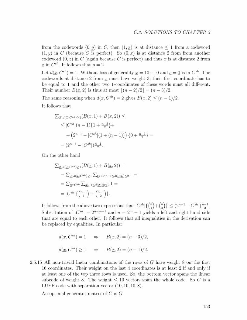
C.3. SOLUTIONS TO CHAPTER 3
from the codewords (0, y) in C, then (1, x) is at distance ≤ 1 from a codeword(1, y) in C (because C is perfect). So (0, x) is at distance 2 from from anothercodeword (0, z) in C (again because C is perfect) and thus x is at distance 2 fromz in Csh. It follows that ρ = 2.
Let d(x,Csh) = 1. Without loss of generality x = 10 · · · 0 and c = 0 is in Csh. Thecodewords at distance 2 from x must have weight 3, their first coordinate has tobe equal to 1 and the other two 1-coordinates of these words must all different.Their number B(x, 2) is thus at most b(n− 2)/2c = (n− 3)/2.
The same reasoning when d(x,Csh) = 2 gives B(x, 2) ≤ (n− 1)/2.
It follows that∑x,d(x,Csh)≥1(B(x, 1) +B(x, 2)) ≤
≤ |Csh|(n− 1){1 + n−32}+
+(2n−1 − |Csh|(1 + (n− 1))
){0 + n−1
2} =
= (2n−1 − |Csh|)n−12.
On the other hand∑x,d(x,Csh)≥1(B(x, 1) +B(x, 2)) =
=∑x,d(x,Csh)≥1
∑c∈Csh, 1≤d(c,x)≤2 1 =
=∑c∈Csh
∑x, 1≤d(x,c)≤2 1 =
= |Csh|{(
n−11
)+(
n−12
)}.
It follows from the above two expressions that |Csh|{(
n1
)+(
n2
)} ≤ (2n−1−|Csh|)n−1
2.
Substitution of |Csh| = 2n−m−1 and n = 2m − 1 yields a left and right hand sidethat are equal to each other. It follows that all inequalities in the derivation canbe replaced by equalities. In particular:
d(x,Csh) = 1 ⇒ B(x, 2) = (n− 3)/2,
d(x,Csh) ≥ 1 ⇒ B(x, 2) = (n− 1)/2.
2.5.15 All non-trivial linear combinations of the rows of G have weight 8 on the first16 coordinates. Their weight on the last 4 coordinates is at least 2 if and only ifat least one of the top three rows is used. So, the bottom vector spans the linearsubcode of weight 8. The weight ≤ 10 vectors span the whole code. So C is aLUEP code with separation vector (10, 10, 10, 8).
An optimal generator matrix of C is G.
153
APPENDIX C. SOLUTIONS TO THE PROBLEMS
C.3 Solutions to Chapter 3
3.4.1 Take the [4, 3, 2] even weight code C1 and the [4, 1, 4] repetition code C2 and applyTheorem 3.1.6.
3.4.2 Let c be a codeword of weight w, w ≥ d. Put it in the top row of a generatormatrix of the code C and permute all the ones of c to the front. One obtains
G =
1 1 · · · 1 0 0 · · · 0
G1 G2
.c of weight w
Then exactly the same proof as of Theorem 3.1.4 yields that the code generated bythe last n− d columns of G, i.e. by G2, has parameters [n−w, k− 1,≥ d−bw/2c]for d ≤ w ≤ 2d − 1. For w ≥ 2d nothing can be said about the dimension orminimum distance of this code.
3.4.3 Again the generator matrix can be assumed to have the form as in the proof ofTheorem 3.1.4, where one may have had to multiply some of the columns by anon-zero constant to get only ones as non-zero elements in the top row. So, again
G =
1 1 · · · 1 0 0 · · · 0
G1 G2
.c of weight d
Let (a1, a2) be a non-trivial linear combination of the last k − 1 rows of G and letuα denote the number of coordinates in a1 equal to α. So
∑α uα = d. Since (a1, a2)
must have distance at least d to αc, one has
(d− uα) + w(a2) ≥ d.
The sum of these inequalities over all α in GF (q) yields qw(a2) ≥ ∑α uα = d, andthus w(a2) ≥ dd/qe. This proves that the residual code of C with respect to aweight d code word has parameters [n− d, k − 1,≥ dd/qe].
3.4.4 Assume that a [101, 7, 50] code exists. Taking successive residual codes with re-spect to minimum weight codewords implies the existence of the following sequenceof codes: [51, 6, 25], [26, 5, 13], [13, 4, 7], [6, 3, 4], [2, 2, 2] and [0, 1, 1]. Howeverthe last code obviously does not exist, so neither does a [101, 7, 50] code.
One can also apply Corollary 3.1.5.
154
C.3. SOLUTIONS TO CHAPTER 3
3.4.5 Clearly, N = n+d−ρ. Also, since d−ρ ≥ 1 it follows that the dimension increasesby 1, i.e. K = k + 1. Finally consider any non-trivial linear combination of therows of the given generator matrix of G∗. If it only involves the top k rows, itsweight is at least d by the assumption on C. If it does involve the bottom row,then the weight of this linear combination is equal to d − ρ plus the distance ofx to a linear combination of the rows of G. This distance is at least ρ, because xhas distance ρ to C. It follows that any non-trivial linear combination of the givengenerator matrix has weight at least d and thus D = d.
We conclude that G∗ is a [n+ d− ρ, k + 1, d] code.
3.4.6 By permuting the columns of the generator matrix G∗ of C∗ one may assumethat the first columns are equal to sT . Since s 6= 0, there must be a row in G∗
that starts with s identical non-zero elements. By permuting the rows of G∗ onecan assume that this is the last row and by a suitable scalar multiplication thisnon-zero element can be assumed to be 1. So we have the following matrix:
G∗ =
s1 · · · s1...
... Gsk · · · sk
1 · · · 1 x1 x2 · · · xn
.
By subtracting si times the last row from row i, 1 ≤ i ≤ k, one can even assumethat s1 = . . . = sk = 0. It follows that G generates an [n, k, d] code C and that xhas distance at least d− s to all codewords in C.
3.4.7 Shortening a linear code with respect to the symbol 0 on coordinate i amounts to:
1) add as row to the parity check matrix the vector that consists of zeros every-where, except for a one at the i-th coordinate,
2) puncture the i-th coordinate in the subcode defined by this new parity checkmatrix (i.e. this subcode consists of all codewords with a zero on the i-th coordi-nate).
Clearly, the new code has parameters [n− 1,≥ k − 1,≥ d].
Since each codeword in C is orthogonal to x, it follows that the subcode of Cconsisting of all codewords that are zero on w − 1 of w one-coordinates of x arealso zero on the w-the coordinate. So, one only has to add w − 1 equations (seefigure below) to the parity check matrix (the dimension of the subcode becomesk−(w−1)) and one obtains w coordinates where all the codewords in this subcodeare zero (so the length becomes n− w).
155
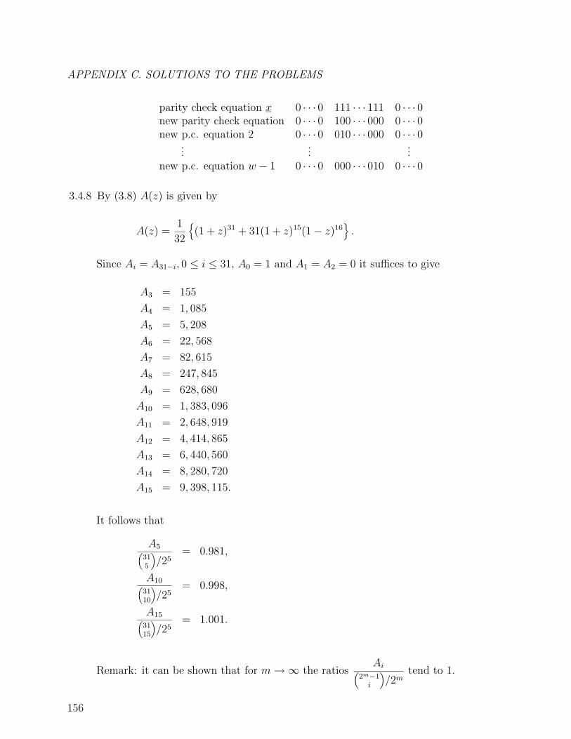
APPENDIX C. SOLUTIONS TO THE PROBLEMS
parity check equation x 0 · · · 0 111 · · · 111 0 · · · 0new parity check equation 0 · · · 0 100 · · · 000 0 · · · 0new p.c. equation 2 0 · · · 0 010 · · · 000 0 · · · 0
......
...new p.c. equation w − 1 0 · · · 0 000 · · · 010 0 · · · 0
3.4.8 By (3.8) A(z) is given by
A(z) =1
32
{(1 + z)31 + 31(1 + z)15(1− z)16
}.
Since Ai = A31−i, 0 ≤ i ≤ 31, A0 = 1 and A1 = A2 = 0 it suffices to give
A3 = 155
A4 = 1, 085
A5 = 5, 208
A6 = 22, 568
A7 = 82, 615
A8 = 247, 845
A9 = 628, 680
A10 = 1, 383, 096
A11 = 2, 648, 919
A12 = 4, 414, 865
A13 = 6, 440, 560
A14 = 8, 280, 720
A15 = 9, 398, 115.
It follows that
A5(315
)/25
= 0.981,
A10(3110
)/25
= 0.998,
A15(3115
)/25
= 1.001.
Remark: it can be shown that for m→∞ the ratiosAi(
2m−1i
)/2m
tend to 1.
156
C.3. SOLUTIONS TO CHAPTER 3
3.4.9 That both codes are perfect follows from Theorem 2.1.7 and the observations
212
{1 +
(23
1
)+
(23
2
)+
(23
3
)}= 223,
36
{1 +
(11
1
)2 +
(11
2
)22
}= 311.
For the recurrence relations of the weight enumerators of these perfect codes wegeneralize the result in equation (3.6).
For the binary perfect [23, 12, 7] code one gets, by observing that each word ofweight q in the vector space must be at distance at most 3 to a unique codeword.(
23w
)= Aw + (w + 1)Aw+1 + (23 − w + 1)Aw−1 +
(w+2
2
)Aw+2 + w(23 − w)Aw +(
23−w+22
)Aw−2 +
(w+3
3
)Aw+3 +
(w+1
2
)(23 − w + 1)Aw+1 + (w + 1)
(23−w+1
2
)Aw−1 +(
23−w+33
)Aw−3,
where the Ai’s are assumed to be zero for i < 0 and i > 23.
Similarly, for the ternary perfect [11, 6, 5] code one gets,(11w
)2w = Aw + (w + 1)Aw+1 + wAw + 2(11 − w + 1)Aw−1 +
(w+2
2
)Aw+2 + (w +
1)wAw+1 +2w(11−w)Aw +(
w2
)Aw +(11−w+1)(w− 1)2Aw−1 +
(11−w+2
2
)22Aw−2,
where one has to realize that there are two ways of changing a zero into a nonzerocoordinate and one way to change a nonzero coordinate into another nonzerocoordinate.
3.4.10 Puncturing a binary [24, 12, 8] code yields a [23, 12,≥ 7] code containing 0. Thiscode is perfect by Theorem 2.1.7 and thus its weight enumerator satisfies therecurrence relation of order seven given in the preceding problem. Since A0 = 1and A1 = . . . = A6 = 0, this recurrence relation has a unique solution.
Consider the 759 codewords of weight 8 in the [24, 12, 8] code and put them in a759× 24 array. Then each column will contain A7 ones and 759− A7 zeros, sincepuncturing that column must yield the codewords of weight 7 and 8.
Counting the number of ones in the array columnwise gives 24A7 but rowwise onegets 759× 8. It follows that A7 = 253 and thus that A8 = 506.
In exactly the same way one gets 24A11 = 2576× 12, and thus A11 = A12 = 1288.Similarly, 24A15 = 759 × 16, and thus A15 = 506 and A16 = 253. From 24A23 =1× 24 it follows that A23 = 1 (of course).
157
APPENDIX C. SOLUTIONS TO THE PROBLEMS
3.4.11 That a (90, 278, 5) binary code has to be perfect follows from Theorem 2.1.7 andthe observation
278
{1 +
(90
1
)+
(90
2
)}= 290.
The recurrence relation for the weight enumerator A(z) of C is given by
(90
w
)= Aw + (w + 1)Aw+1 + (90− w + 1)Aw−1 +
+
(w + 2
2
)Aw+2 + w(90− w)Aw +
+
(90− w + 2
2
)Aw−2.
Let c be one of the codewords in C. Translate the C over −c. One obtains a newcode with the same parameters (thus also perfect) containing 0. So, the weightenumerator of this code obviously satisfies A0 = 1, A1 = . . . = A4 = 0. For theother coefficients we use the recurrence relation with w = 3, 4 and 5.
Substitution of w = 3 in the recurrence relation yields:(
903
)=(
52
)A5, and thus
A5 = 11748.
Substitution of w = 4 in the recurrence relation yields:(
904
)=(
62
)A6 + 5A5, and
thus A6 = 166430.
Substitution of w = 5 in the recurrence relation yields:(
905
)=(
72
)A7 + 6A6 + 5×
85A5, and thus A7 = 180751357.
Since the coefficient Aw in the weight enumerator of a code counts the number ofcodewords of weight w this number has to be an integer. From the fact that A7
is not an integer we can conclude that a binary (perfect) (90, 278, 5) code does notexist.
3.4.12 Consider the Boolean function∑
1≤i<j≤m aijxixj+∑
1≤i≤m bixi+c with at least oneof the a′ijs not equal to 0. We first want to demonstrate that a suitable invertibleaffine transformation maps this function to one of exactly the same form but witha12 6= 0.
If a12 = 1 there is nothing to do. If a1j = 1 with j > 2 apply x′2 = xj, x′j = x2 and
x′k = xk for k 6= 2, j. If ai2 = 1 with i > 2, interchange x1 and xi in a similar way.Finally, if a1k = 0 for all k and ak2 = 0 for all k while aij = 1, apply the mappingthat interchanges both 1 and i and 1 and j.
Now∑
1≤i<j≤m aijxixj +∑
1≤i≤m bixi + c with a12 = 1 can be rewritten as
158
C.3. SOLUTIONS TO CHAPTER 3
(x1 +∑
i≥3 a2ixi + b2)(x2 +∑
j≥3 a1jxj + b1) + (∑
i≥3 a2ixi + b2)(∑
j≥3 a1jxj + b1) +∑3≤i<j≤m aijxixj +
∑3≤i≤m bixi + c.
This means that the invertible affine transformation
x′1 = x1 +∑
i≥3 a2ixi + b2,x′2 = x2 +
∑j≥3 a1jxi + b1,
x′k = xk, k ≥ 3,
transforms the above function into
x1x2 +∑
3≤i<j≤m
aijxixj +∑
3≤i≤m
bixi + c,
where we have left out all primes in the notation.
Note that the product of several invertible affine transformations, one applied oneafter another, still is an invertible affine transformation.
If one of the terms aij with 3 ≤ i < j ≤ m is not equal to 1, one can findin exactly the same way an invertible affine transformation that yields the formx1x2+x3x4+
∑4≤i<j≤m aijxixj +
∑4≤i≤m bixi +c Continuing in this way one arrives
at
x1x2 + · · ·+ x2l−1x2l +∑
2l+1≤i≤m
bixi + c.
If one of the bi 6= 0, i ≥ 2l + 1, one can apply an invertible affine transformationthat maps the above form into x1x2+· · ·+x2l−1x2l+x2l+1. So the following standardforms can be found:
1) 02) 13) x1
4) x1x2 + . . .+ x2l−1x2l, 2l ≤ m,5) x1x2 + . . .+ x2l−1x2l + 1, , 2l ≤ m,6) x1x2 + . . .+ x2l−1x2l + x2l+1, , 2l + 1 ≤ m.
It follows from the above that each word in RM(2, 5) can be mapped by aninvertible affine transformation into one of the following words: 0, 1, x1, x1x2,x1x2 + x3x4, x1x2 + 1, x1x2 + x3x4 + 1, x1x2 + x3 or x1x2 + x3x4 + x5.
Since an invertible affine transformation permutes the coordinates, such a trans-formation will not affect the weight of words. So, as one can easliy check, thesestandard forms give rise to the following weights:
159
APPENDIX C. SOLUTIONS TO THE PROBLEMS
weight standardforms0 08 x1x2
12 x1x2 + x3x4
16 x1
x1x2 + x3
x1x2 + x3x4 + x5
20 x1x2 + x3x4 + 124 x1x2 + 132 1
For instance, x1x2 is equal to 1 if and only if x1 = x2 = 1, independent of thevalues of x3, x4 and x5, i.e. independent of the eight possible values of (x3, x4, x5).
That RM(2, 5) is a selfdual code follows directly from Theorem 3.3.4. If followsthat the weight enumerator of RM(2, 5) is equal to that of its dual code. Thereare only five unknown coefficients: A8, A12, A16, A20 and A24. Comparing the co-efficients of zi, 0 ≤ 7, in the MacWilliams relations (Theorem 2.3.4) will yield allthese coefficients.
3.4.13 The coefficient a13 is given by the innerproduct of c with any of the eight products(x2 +u2)(x4 +u4)(x5 +u5). The choice u2 = u4 = u5 = 1 results in the coordinateswith x2 = x4 = x5 = 0, i.e. coordinates 0, 4, 16 and 20. In other words a13 =c0 + c4 + c16 + c20. Together with the other choices of u2, u4 and u5 one gets thefollowing equalities.
a13 = c0 + c4 + c16 + c20a13 = c1 + c5 + c17 + c21a13 = c2 + c6 + c18 + c22a13 = c3 + c7 + c19 + c23a13 = c8 + c12 + c24 + c28a13 = c9 + c13 + c25 + c29a13 = c10 + c14 + c26 + c30a13 = c11 + c15 + c27 + c31
.
Similarly for a3 one finds that it should be equal to each of: c0 + c4, c1 + c5, c2 + c6,c3 + c7, c8 + c12, c9 + c13, c10 + c14, c11 + c15, c16 + c20, c17 + c21, c18 + c22, c19 + c23c24 + c28, c25 + c29, c26 + c30, c27 + c31 (the primes in c′i have been left out).
Finally for a∅ one has the 32 equations a∅ = ci, 0 ≤ i ≤ 31 (the primes in c′′i havebeen left out).
160

C.4. SOLUTIONS TO CHAPTER 4
C.4 Solutions to Chapter 4
4.7.1 If f and g are q-ary polynomials of degree less than k and u and v are elementsin GF (q), then also uf + vg is a q-ary polynomial of degree degree less than k. SoC is a linear code. That the dimension of C is k follows from the fact that theonly polynomial of degree less than n that is identical to zero on all the non-zeroelements of GF (q) is the polynomial 0. Since there are qk polynomials of degreeless than k, one can conclude that C is a k-dimensional code.
Any non-zero polynomial of degree less than k has at most k − 1 zeros, so eachnon-zero vector in C has weight at least n−(k−1). So, C is an [n, k, d ≥ n−k+1]code. From (2.17) it follows that d = n− k + 1 and that C is an MDS code.
The polynomials xi, 0 ≤ i < k, give rise to the following base of the code C overGF (q):
(1, αi, . . . , αi(n−1)), 0 ≤ i < k.
Cyclically shifting the i-th vector yields (αi, α2i, . . . , αi(n−1), αin), which can bewritten as αi(1, αi, . . . , αi(n−1)). This vector also lies in C and is the image of thepolynomial αixi. It follows that the cyclic shifts of the basis vectors are again inthe code and also generate it, so C is cyclic. To make this more explicit: the cyclicshift of the codeword defined by the polynomial f(x) is the codeword defined bythe polynomial f(αx), which is of the same degree as f(x) is.
In fact C is the Reed Solomon code.
4.7.2 Let α be a primitive 11-th root of unity in an extension field of GF (3). Thenx11 − 1 = (x − 1)(x − α) . . . (x − α10). Let m1(x) be the minimal polynomial ofα. Then the conjugates of α are α3, α9, α27 = α5 and α15 = α4. Similarly theconjugates of α−1 = α10 are α8, α2, α6 and α7.
So the factorization of x11 − 1 over GF (3) is given by
x11 − 1 = (x− 1)m1(x)m−1(x),
with
m1(x) = (x− α)(x− α3)(x− α9)(x− α5)(x− α4)
m−1(x) = (x− α10)(x− α8)(x− α2)(x− α6)(x− α7),
both of degree 5.
The smallest extension field of GF (3) that contains a primitive 11-th root of unityis GF (3m), with m minimal such that 11 divides 3m − 1, so m = 5.
Let ω be a primitive element in GF (35). Then α = ω(35−1)/11 is a primitive 11-throot of unity in GF (35). So the zeros of m1(x) are ω22, ω66, ω198, ω110, ω88, those ofm−1(x) are ω220, ω176, ω44, ω132, ω154.
161

APPENDIX C. SOLUTIONS TO THE PROBLEMS
4.7.3 Let α be a primitive, 93-th root of unity in an extension field of GF (2). Thegenerator polynomial g(x) must have αi, 1 ≤ i ≤ 12, as zeros. Grouping theconjugates of these zeros in their cyclotomic cosets, one gets:
cyclotomic cosets exponents i of the zeros αi
C1 1, 2, 4, 8, 16, 32, 64, 35, 70, 47C3 3, 6, 12, 24, 48C5 5, 10, 20, 40, 80, 67, 41, 82, 71, 49C7 7, 14, 28, 56, 19, 38, 76, 59, 25, 50C9 9, 18, 36, 72, 51C11 11, 22, 44, 88, 83, 73, 53, 13, 26, 52
The dimension of C is 93 minus the number of zeros, so it is 93−4×10−2×5 = 43.
Since g(x) also has α13 and α14 as zeros, the actual minimum distance will be atleast 15 by the BCH bound.
4.7.4 The generator polynomial g(x) of C must have αi, 1 ≤ i ≤ 4, as zeros, whereα is a primitive 15-th root of unity. So, g(x) = m1(x)m3(x), with m1(x) =(x− α)(x− α2)(x− α4)(x− α8) and m3(x) = (x− α3)(x− α6)(x− α12)(x− α9).
The smallest extension field of GF (2) that contains a primitive 15-th root of unityis GF (24). If GF (24) is represented as GF (2)[x]/(x4+x+1), one has that m1(x) =x4 + x+ 1 and m3(x) = x4 + x3 + x2 + x+ 1, so g(x) = 1 + x4 + x6 + x7 + x8.
4.7.5 Since the smallest m for which 33 divides 2m− 1 is 10, the smallest extension fieldof GF (2) containing α is GF (210).
The cyclotomic coset C1 containing 1 has as elements 1, 2, 4, 8, 16, −1, −2, −4,−8, −16. Together with C0 = {0} one has 11 zeros of the generator polynomialg(x). So the dimension of C is 33− 11 = 22.
The generator polynomial has the five consecutive zeros αi, − 2 ≤ i ≤ 2, so theBCH bound gives that d ≥ 6.
If d = 7 or more, one gets a contradiction with the Hamming bound (Theorem2.1.3), since
3∑i=0
(33
i
)= 6018 > 211.
4.7.6 The conjugates of α are α, α2, α4, α8, and those of α3 are α3, α6, α12, α9. So thegenerator polynomial g(x) has the four consecutive zeros: α, α2, α3, α4 and thusthe the minimum distance d is at least 5 by the BCH-bound.
Now consider the syndrome s1 = α7 and s3 = α14. We follow Algorithm 4.2.3.Note that s3 6= s3
1. With a logarithm table of GF (2)[x]/(x4 + x + 1) one can findthat (s3 + s3
1)/s1 = (α14 + α6)/α7 = α.
162
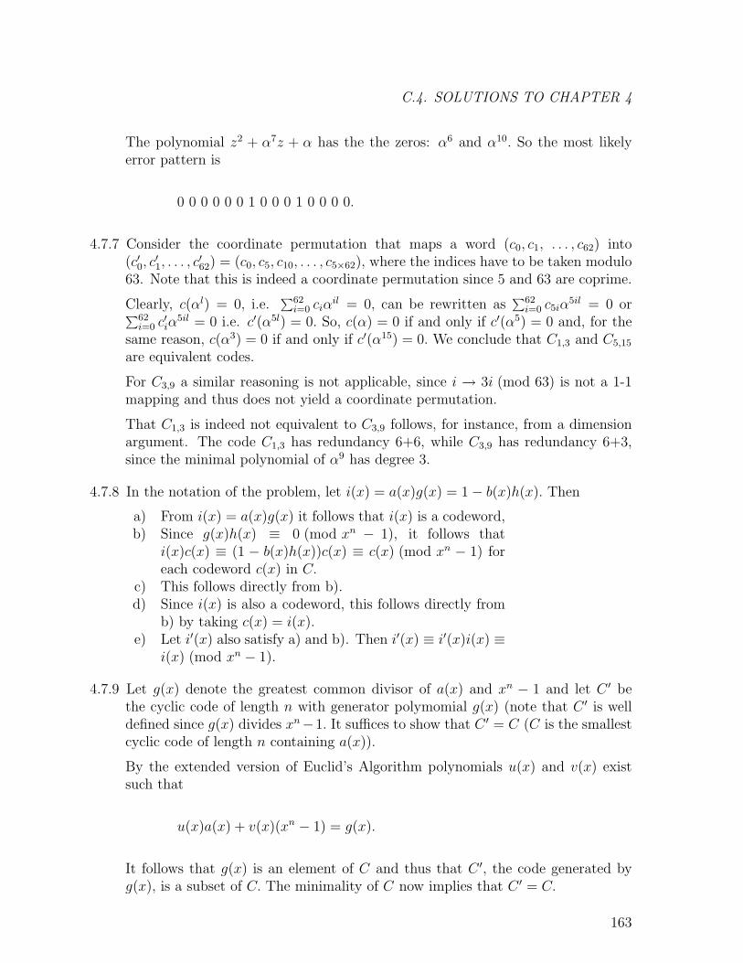
C.4. SOLUTIONS TO CHAPTER 4
The polynomial z2 + α7z + α has the the zeros: α6 and α10. So the most likelyerror pattern is
0 0 0 0 0 0 1 0 0 0 1 0 0 0 0.
4.7.7 Consider the coordinate permutation that maps a word (c0, c1, . . . , c62) into(c′0, c
′1, . . . , c
′62) = (c0, c5, c10, . . . , c5×62), where the indices have to be taken modulo
63. Note that this is indeed a coordinate permutation since 5 and 63 are coprime.
Clearly, c(αl) = 0, i.e.∑62
i=0 ciαil = 0, can be rewritten as
∑62i=0 c5iα
5il = 0 or∑62i=0 c
′iα
5il = 0 i.e. c′(α5l) = 0. So, c(α) = 0 if and only if c′(α5) = 0 and, for thesame reason, c(α3) = 0 if and only if c′(α15) = 0. We conclude that C1,3 and C5,15
are equivalent codes.
For C3,9 a similar reasoning is not applicable, since i → 3i (mod 63) is not a 1-1mapping and thus does not yield a coordinate permutation.
That C1,3 is indeed not equivalent to C3,9 follows, for instance, from a dimensionargument. The code C1,3 has redundancy 6+6, while C3,9 has redundancy 6+3,since the minimal polynomial of α9 has degree 3.
4.7.8 In the notation of the problem, let i(x) = a(x)g(x) = 1− b(x)h(x). Then
a) From i(x) = a(x)g(x) it follows that i(x) is a codeword,b) Since g(x)h(x) ≡ 0 (mod xn − 1), it follows that
i(x)c(x) ≡ (1 − b(x)h(x))c(x) ≡ c(x) (mod xn − 1) foreach codeword c(x) in C.
c) This follows directly from b).d) Since i(x) is also a codeword, this follows directly from
b) by taking c(x) = i(x).e) Let i′(x) also satisfy a) and b). Then i′(x) ≡ i′(x)i(x) ≡
i(x) (mod xn − 1).
4.7.9 Let g(x) denote the greatest common divisor of a(x) and xn − 1 and let C ′ bethe cyclic code of length n with generator polymomial g(x) (note that C ′ is welldefined since g(x) divides xn−1. It suffices to show that C ′ = C (C is the smallestcyclic code of length n containing a(x)).
By the extended version of Euclid’s Algorithm polynomials u(x) and v(x) existsuch that
u(x)a(x) + v(x)(xn − 1) = g(x).
It follows that g(x) is an element of C and thus that C ′, the code generated byg(x), is a subset of C. The minimality of C now implies that C ′ = C.
163
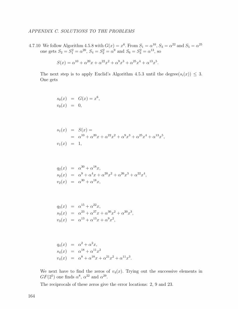
APPENDIX C. SOLUTIONS TO THE PROBLEMS
4.7.10 We follow Algorithm 4.5.8 with G(x) = x6. From S1 = α10, S3 = α22 and S5 = α25
one gets S2 = S21 = α20, S4 = S2
2 = α9 and S6 = S23 = α13, so
S(x) = α10 + α20x+ α22x2 + α9x3 + α25x4 + α13x5.
The next step is to apply Euclid’s Algorithm 4.5.3 until the degree(si(x)) ≤ 3.One gets
s0(x) = G(x) = x6,
v0(x) = 0,
s1(x) = S(x) =
= α10 + α20x+ α22x2 + α9x3 + α25x4 + α13x5,
v1(x) = 1,
q2(x) = α30 + α18x,
s2(x) = α9 + α4x+ α20x2 + α26x3 + α22x4,
v2(x) = α30 + α18x,
q3(x) = α15 + α22x,
s3(x) = α23 + α27x+ α30x2 + α20x3,
v3(x) = α13 + α13x+ α9x2,
q4(x) = α2 + α2x,
s4(x) = α18 + α11x2
v4(x) = α8 + α18x+ α21x2 + α11x3.
We next have to find the zeros of v4(x). Trying out the successive elements inGF (25) one finds α8, α22 and α29.
The reciprocals of these zeros give the error locations: 2, 9 and 23.
164
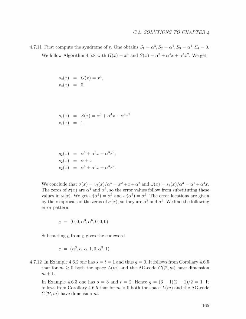
C.4. SOLUTIONS TO CHAPTER 4
4.7.11 First compute the syndrome of r. One obtains S1 = α3, S2 = α4, S3 = α4, S4 = 0.
We follow Algorithm 4.5.8 with G(x) = x4 and S(x) = α3 + α4x+ α4x2. We get:
s0(x) = G(x) = x4,
v0(x) = 0,
s1(x) = S(x) = α3 + α4x+ α4x2
v1(x) = 1,
q2(x) = α5 + α3x+ α3x2,
s2(x) = α+ x
v2(x) = α5 + α3x+ α3x2.
We conclude that σ(x) = v2(x)/α3 = x2 +x+α2 and ω(x) = s2(x)/α
3 = α5 +α4x.The zeros of σ(x) are α4 and α5, so the error values follow from substituting thesevalues in ω(x). We get ω(α4) = α6 and ω(α5) = α3. The error locations are givenby the reciprocals of the zeros of σ(x), so they are α2 and α3. We find the followingerror pattern:
e = (0, 0, α3, α6, 0, 0, 0).
Subtracting e from r gives the codeword
c = (α3, α, α, 1, 0, α3, 1).
4.7.12 In Example 4.6.2 one has s = t = 1 and thus g = 0. It follows from Corollary 4.6.5that for m ≥ 0 both the space L(m) and the AG-code C(P ,m) have dimensionm+ 1.
In Example 4.6.3 one has s = 3 and t = 2. Hence g = (3 − 1)(2 − 1)/2 = 1. Itfollows from Corollary 4.6.5 that for m > 0 both the space L(m) and the AG-codeC(P ,m) have dimension m.
165
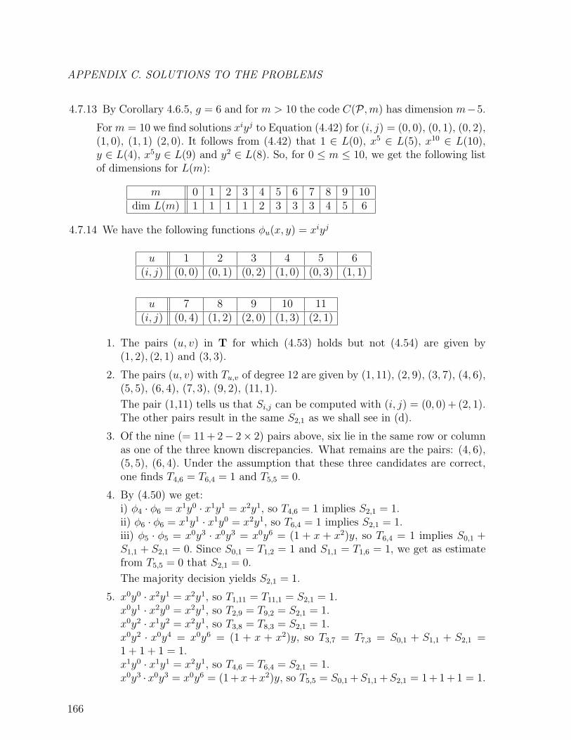
APPENDIX C. SOLUTIONS TO THE PROBLEMS
4.7.13 By Corollary 4.6.5, g = 6 and for m > 10 the code C(P ,m) has dimension m−5.
For m = 10 we find solutions xiyj to Equation (4.42) for (i, j) = (0, 0), (0, 1), (0, 2),(1, 0), (1, 1) (2, 0). It follows from (4.42) that 1 ∈ L(0), x5 ∈ L(5), x10 ∈ L(10),y ∈ L(4), x5y ∈ L(9) and y2 ∈ L(8). So, for 0 ≤ m ≤ 10, we get the following listof dimensions for L(m):
m 0 1 2 3 4 5 6 7 8 9 10dim L(m) 1 1 1 1 2 3 3 3 4 5 6
4.7.14 We have the following functions φu(x, y) = xiyj
u 1 2 3 4 5 6(i, j) (0, 0) (0, 1) (0, 2) (1, 0) (0, 3) (1, 1)
u 7 8 9 10 11(i, j) (0, 4) (1, 2) (2, 0) (1, 3) (2, 1)
1. The pairs (u, v) in T for which (4.53) holds but not (4.54) are given by(1, 2), (2, 1) and (3, 3).
2. The pairs (u, v) with Tu,v of degree 12 are given by (1, 11), (2, 9), (3, 7), (4, 6),(5, 5), (6, 4), (7, 3), (9, 2), (11, 1).
The pair (1,11) tells us that Si,j can be computed with (i, j) = (0, 0) + (2, 1).The other pairs result in the same S2,1 as we shall see in (d).
3. Of the nine (= 11 + 2− 2× 2) pairs above, six lie in the same row or columnas one of the three known discrepancies. What remains are the pairs: (4, 6),(5, 5), (6, 4). Under the assumption that these three candidates are correct,one finds T4,6 = T6,4 = 1 and T5,5 = 0.
4. By (4.50) we get:i) φ4 · φ6 = x1y0 · x1y1 = x2y1, so T4,6 = 1 implies S2,1 = 1.ii) φ6 · φ6 = x1y1 · x1y0 = x2y1, so T6,4 = 1 implies S2,1 = 1.iii) φ5 · φ5 = x0y3 · x0y3 = x0y6 = (1 + x + x2)y, so T6,4 = 1 implies S0,1 +S1,1 + S2,1 = 0. Since S0,1 = T1,2 = 1 and S1,1 = T1,6 = 1, we get as estimatefrom T5,5 = 0 that S2,1 = 0.
The majority decision yields S2,1 = 1.
5. x0y0 · x2y1 = x2y1, so T1,11 = T11,1 = S2,1 = 1.x0y1 · x2y0 = x2y1, so T2,9 = T9,2 = S2,1 = 1.x0y2 · x1y2 = x2y1, so T3,8 = T8,3 = S2,1 = 1.x0y2 · x0y4 = x0y6 = (1 + x + x2)y, so T3,7 = T7,3 = S0,1 + S1,1 + S2,1 =1 + 1 + 1 = 1.x1y0 · x1y1 = x2y1, so T4,6 = T6,4 = S2,1 = 1.x0y3 ·x0y3 = x0y6 = (1+x+x2)y, so T5,5 = S0,1 +S1,1 +S2,1 = 1+1+1 = 1.
166
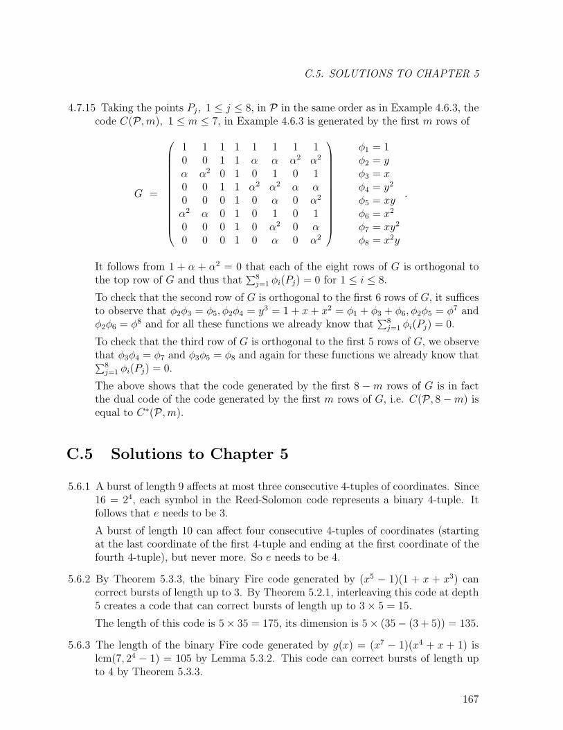
C.5. SOLUTIONS TO CHAPTER 5
4.7.15 Taking the points Pj, 1 ≤ j ≤ 8, in P in the same order as in Example 4.6.3, thecode C(P ,m), 1 ≤ m ≤ 7, in Example 4.6.3 is generated by the first m rows of
G =
1 1 1 1 1 1 1 10 0 1 1 α α α2 α2
α α2 0 1 0 1 0 10 0 1 1 α2 α2 α α0 0 0 1 0 α 0 α2
α2 α 0 1 0 1 0 10 0 0 1 0 α2 0 α0 0 0 1 0 α 0 α2
φ1 = 1φ2 = yφ3 = xφ4 = y2
φ5 = xyφ6 = x2
φ7 = xy2
φ8 = x2y
.
It follows from 1 + α + α2 = 0 that each of the eight rows of G is orthogonal tothe top row of G and thus that
∑8j=1 φi(Pj) = 0 for 1 ≤ i ≤ 8.
To check that the second row of G is orthogonal to the first 6 rows of G, it sufficesto observe that φ2φ3 = φ5, φ2φ4 = y3 = 1 + x+ x2 = φ1 + φ3 + φ6, φ2φ5 = φ7 andφ2φ6 = φ8 and for all these functions we already know that
∑8j=1 φi(Pj) = 0.
To check that the third row of G is orthogonal to the first 5 rows of G, we observethat φ3φ4 = φ7 and φ3φ5 = φ8 and again for these functions we already know that∑8
j=1 φi(Pj) = 0.
The above shows that the code generated by the first 8 −m rows of G is in factthe dual code of the code generated by the first m rows of G, i.e. C(P , 8−m) isequal to C∗(P ,m).
C.5 Solutions to Chapter 5
5.6.1 A burst of length 9 affects at most three consecutive 4-tuples of coordinates. Since16 = 24, each symbol in the Reed-Solomon code represents a binary 4-tuple. Itfollows that e needs to be 3.
A burst of length 10 can affect four consecutive 4-tuples of coordinates (startingat the last coordinate of the first 4-tuple and ending at the first coordinate of thefourth 4-tuple), but never more. So e needs to be 4.
5.6.2 By Theorem 5.3.3, the binary Fire code generated by (x5 − 1)(1 + x + x3) cancorrect bursts of length up to 3. By Theorem 5.2.1, interleaving this code at depth5 creates a code that can correct bursts of length up to 3× 5 = 15.
The length of this code is 5× 35 = 175, its dimension is 5× (35− (3 + 5)) = 135.
5.6.3 The length of the binary Fire code generated by g(x) = (x7 − 1)(x4 + x + 1) islcm(7, 24 − 1) = 105 by Lemma 5.3.2. This code can correct bursts of length upto 4 by Theorem 5.3.3.
167
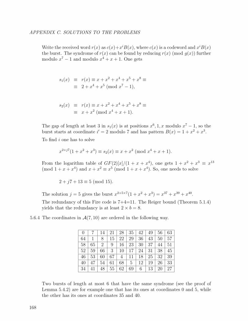
APPENDIX C. SOLUTIONS TO THE PROBLEMS
Write the received word r(x) as c(x)+xiB(x), where c(x) is a codeword and xiB(x)the burst. The syndrome of r(x) can be found by reducing r(x) (mod g(x)) furthermodulo x7 − 1 and modulo x4 + x+ 1. One gets
s1(x) ≡ r(x) ≡ x+ x2 + x4 + x5 + x8 ≡≡ 2 + x4 + x5 (mod x7 − 1),
s2(x) ≡ r(x) ≡ x+ x2 + x4 + x5 + x8 ≡≡ x+ x2 (mod x4 + x+ 1).
The gap of length at least 3 in s1(x) is at positions x6, 1, x modulo x7 − 1, so theburst starts at coordinate i′ = 2 modulo 7 and has pattern B(x) = 1 + x2 + x3.
To find i one has to solve
x2+j7(1 + x2 + x3) ≡ s2(x) ≡ x+ x2 (mod x4 + x+ 1).
From the logarithm table of GF (2)[x]/(1 + x + x4), one gets 1 + x2 + x3 ≡ x13
(mod 1 + x+ x4) and x+ x2 ≡ x5 (mod 1 + x+ x4). So, one needs to solve
2 + j7 + 13 ≡ 5 (mod 15).
The solution j = 5 gives the burst x2+5×7(1 + x2 + x3) = x37 + x39 + x40.
The redundancy of this Fire code is 7+4=11. The Reiger bound (Theorem 5.1.4)yields that the redundancy is at least 2× b = 8.
5.6.4 The coordinates in A(7, 10) are ordered in the following way.
0 7 14 21 28 35 42 49 56 6364 1 8 15 22 29 36 43 50 5758 65 2 9 16 23 30 37 44 5152 59 66 3 10 17 24 31 38 4546 53 60 67 4 11 18 25 32 3940 47 54 61 68 5 12 19 26 3334 41 48 55 62 69 6 13 20 27
Two bursts of length at most 6 that have the same syndrome (see the proof ofLemma 5.4.2) are for example one that has its ones at coordinates 0 and 5, whilethe other has its ones at coordinates 35 and 40.
168
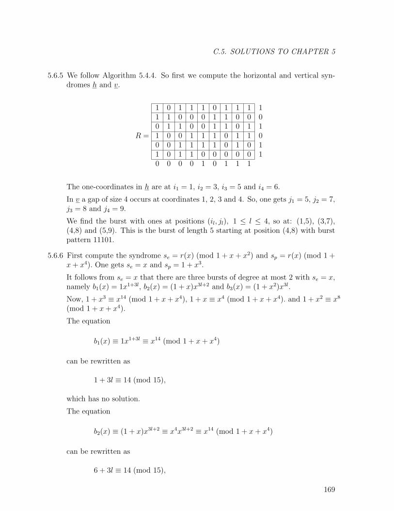
C.5. SOLUTIONS TO CHAPTER 5
5.6.5 We follow Algorithm 5.4.4. So first we compute the horizontal and vertical syn-dromes h and v.
R =
1 0 1 1 1 0 1 1 1 11 1 0 0 0 1 1 0 0 00 1 1 0 0 1 1 0 1 11 0 0 1 1 1 0 1 1 00 0 1 1 1 1 0 1 0 11 0 1 1 0 0 0 0 0 10 0 0 0 1 0 1 1 1
The one-coordinates in h are at i1 = 1, i2 = 3, i3 = 5 and i4 = 6.
In v a gap of size 4 occurs at coordinates 1, 2, 3 and 4. So, one gets j1 = 5, j2 = 7,j3 = 8 and j4 = 9.
We find the burst with ones at positions (il, jl), 1 ≤ l ≤ 4, so at: (1,5), (3,7),(4,8) and (5,9). This is the burst of length 5 starting at position (4,8) with burstpattern 11101.
5.6.6 First compute the syndrome se = r(x) (mod 1 + x + x2) and sp = r(x) (mod 1 +x+ x4). One gets se = x and sp = 1 + x3.
It follows from se = x that there are three bursts of degree at most 2 with se = x,namely b1(x) = 1x1+3l, b2(x) = (1 + x)x3l+2 and b3(x) = (1 + x2)x3l.
Now, 1 + x3 ≡ x14 (mod 1 + x+ x4), 1 + x ≡ x4 (mod 1 + x+ x4). and 1 + x2 ≡ x8
(mod 1 + x+ x4).
The equation
b1(x) ≡ 1x1+3l ≡ x14 (mod 1 + x+ x4)
can be rewritten as
1 + 3l ≡ 14 (mod 15),
which has no solution.
The equation
b2(x) ≡ (1 + x)x3l+2 ≡ x4x3l+2 ≡ x14 (mod 1 + x+ x4)
can be rewritten as
6 + 3l ≡ 14 (mod 15),
169

APPENDIX C. SOLUTIONS TO THE PROBLEMS
which has no solution.
The equation
b3(x) ≡ (1 + x2)x3l ≡ x8x3l ≡ x14 (mod 1 + x+ x4)
can be rewritten as
8 + 3l ≡ 14 (mod 15),
which has l ≡ 2 (mod 5) as solution.
We conclude that the burst of length (1 + x2)x6 has occurred and that the trans-mitted codeword is r(x)− (1 + x2)x6 = 1 + x2 + x4 + x8 + x10 + x13 + x14.
5.6.7 Since e(x) = 1 + x3 has period 3 = 22− 1 it follows that the generator polynomialg(x) must have the form g(x) = (1 + x3)p(x), with p(x) is a primitive polynomialof even degree m.
Possible burst patterns of length at most 4, that are not the product of smallerdegree patterns are: 1, 1 + x, 1 + x+ x2, 1 + x+ x3 and 1 + x2 + x3.
Define a, b, c and d by
1 + x ≡ xa (mod p(x)),1 + x+ x2 ≡ xb (mod p(x)),1 + x+ x3 ≡ xc (mod p(x)),
1 + x2 + x3 ≡ xd (mod p(x)).
Consider the burst patterns B1(x) = 1 and B2(x) = 1 + x + x3. Clearly,B1(x) ≡ xlB2(x) (mod 1 + x3), i.e. 1 ≡ xl(1 + x + x3) (mod 1 + x3) if and onlyif l ≡ 2 (mod 3). From the condition B1(x) 6≡ xlB2(x) (mod p(x)), i.e. 1 6≡ xlxc
(mod p(x)) for all l ≡ 2 (mod 3) it now follows that 0 6≡ 2 + c (mod 3), i.e. c 6≡ 2(mod 3).
Similarly, the burst patterns B1(x) = 1 and B2(x) = 1+x2+x3 yield the conditiond 6≡ 2 (mod 3).
The burst patterns B1(x) = 1+x and B2(x) = 1+x2 = (1+x)2 yield the conditiona 6≡ 1 + 2a (mod 3) and thus a 6≡ 2 (mod 3).
The burst patterns B1(x) = 1+x+x3 and B2(x) = 1+x2 +x3 yield the conditionc 6≡ 2 + d (mod 3) and thus c+ 2d 6≡ 2 (mod 3).
It just so turns out that none of the other burst patterns give rise to furtherrelations, so that we have the following AES conditions in the a, c and d definedabove (and not in b):
170
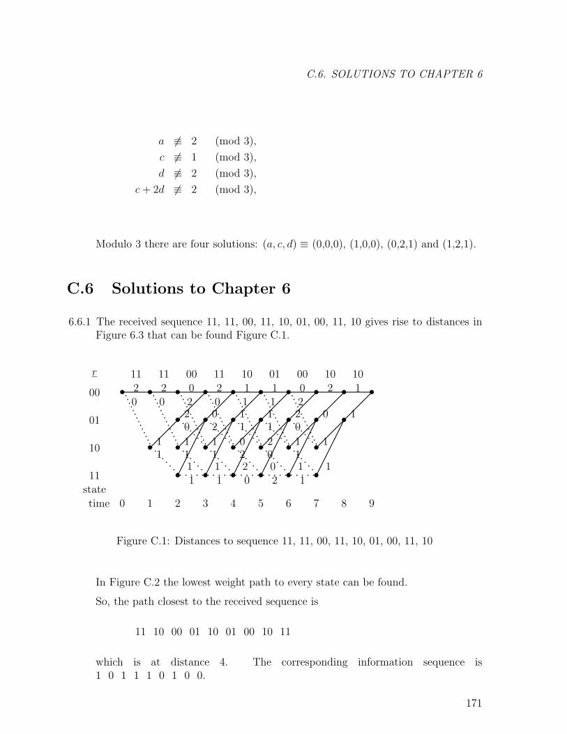
C.6. SOLUTIONS TO CHAPTER 6
a 6≡ 2 (mod 3),
c 6≡ 1 (mod 3),
d 6≡ 2 (mod 3),
c+ 2d 6≡ 2 (mod 3),
Modulo 3 there are four solutions: (a, c, d) ≡ (0,0,0), (1,0,0), (0,2,1) and (1,2,1).
C.6 Solutions to Chapter 6
6.6.1 The received sequence 11, 11, 00, 11, 10, 01, 00, 11, 10 gives rise to distances inFigure 6.3 that can be found Figure C.1.
• • • • • • • • • •
• • • • • • •
• • • • • • •
• • • • • •
��
�
��
�
��
�
��
�
��
�
��
�
��
�
��
�
��
�
��
�
��
�
��
�
��
�
��
�
������
������
������
������
������
������
················
················
················
················
················
················
················
········
········
········
········
················
········
········
········
········
········· · · · · · · · · · · · · · · · · · · · · · · · ·
00
01
10
11state
time
r 11 11 00 11 10 01 00 10 10
0 1 2 3 4 5 6 7 8 9
20
20
11
0 22 02 00 2
1 11 11 11 1
1 11 11 11 1
0 22 02 00 2
0 222 00
1 111 11
1
1
Figure C.1: Distances to sequence 11, 11, 00, 11, 10, 01, 00, 11, 10
In Figure C.2 the lowest weight path to every state can be found.
So, the path closest to the received sequence is
11 10 00 01 10 01 00 10 11
which is at distance 4. The corresponding information sequence is1 0 1 1 1 0 1 0 0.
171
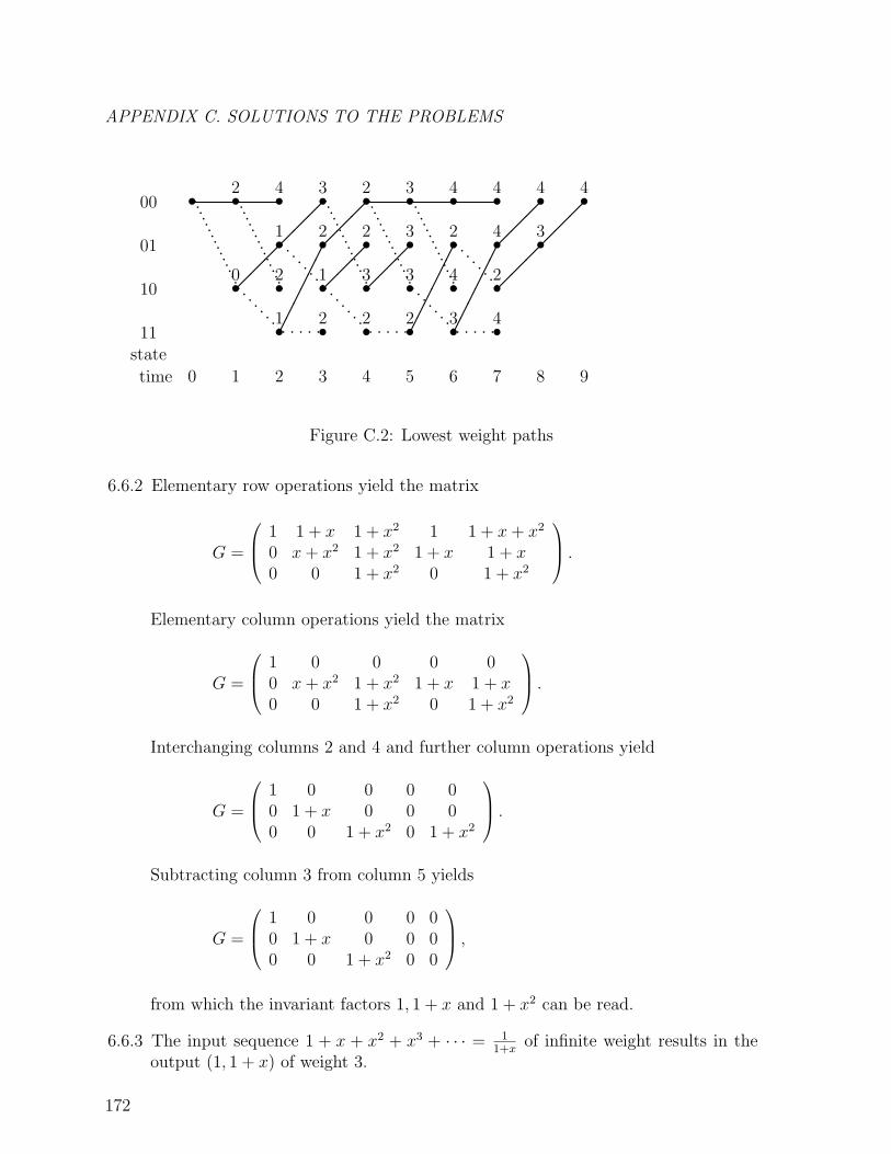
APPENDIX C. SOLUTIONS TO THE PROBLEMS
• • • • • • • • • •
• • • • • • •
• • • • • • •
• • • • • •
················
················��
�
········
················
················
················��
�
��
�
········
········
��
�
��
�
��
�
········
········
· · · · · · · · · · · · · · ·������
������
�������
��
��
�
00
01
10
11state
time
2
0
4
1
2
1
3
2
1
2
2
2
3
2
3
3
3
2
4
2
4
3
4
4
2
4
4
3
4
0 1 2 3 4 5 6 7 8 9
Figure C.2: Lowest weight paths
6.6.2 Elementary row operations yield the matrix
G =
1 1 + x 1 + x2 1 1 + x+ x2
0 x+ x2 1 + x2 1 + x 1 + x0 0 1 + x2 0 1 + x2
.Elementary column operations yield the matrix
G =
1 0 0 0 00 x+ x2 1 + x2 1 + x 1 + x0 0 1 + x2 0 1 + x2
.Interchanging columns 2 and 4 and further column operations yield
G =
1 0 0 0 00 1 + x 0 0 00 0 1 + x2 0 1 + x2
.Subtracting column 3 from column 5 yields
G =
1 0 0 0 00 1 + x 0 0 00 0 1 + x2 0 0
,from which the invariant factors 1, 1 + x and 1 + x2 can be read.
6.6.3 The input sequence 1 + x + x2 + x3 + · · · = 11+x
of infinite weight results in theoutput (1, 1 + x) of weight 3.
172
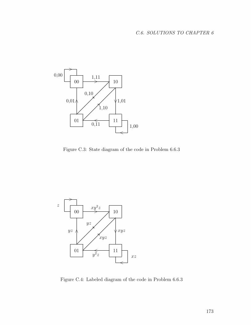
C.6. SOLUTIONS TO CHAPTER 6
01 11
00 10
��
��
��
��
��
��
��
��
1,11>
0,11<
1,01∨0,01∧
1,00
<
0,00>
0,10
1,10
Figure C.3: State diagram of the code in Problem 6.6.3
01 11
00 10
��
��
��
��
��
��
��
��
xy2z>
y2z<
xyz∨yz ∧
xz
<
z>
yz
xyz
Figure C.4: Labeled diagram of the code in Problem 6.6.3
173
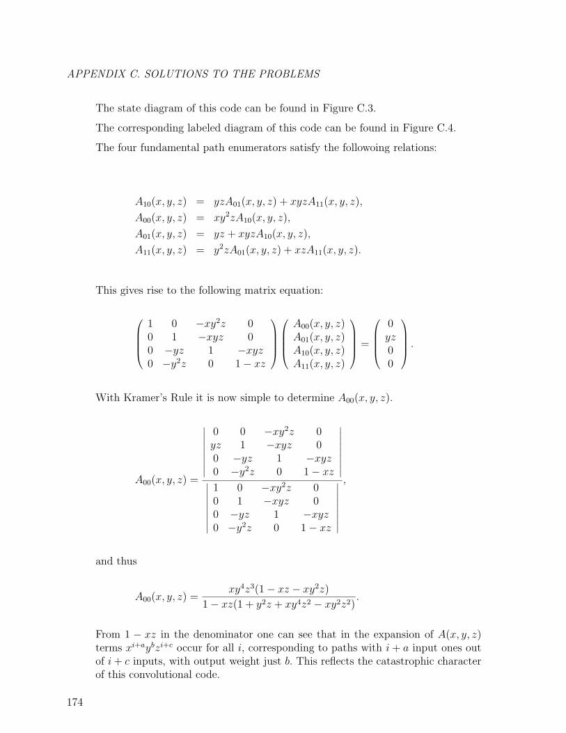
APPENDIX C. SOLUTIONS TO THE PROBLEMS
The state diagram of this code can be found in Figure C.3.
The corresponding labeled diagram of this code can be found in Figure C.4.
The four fundamental path enumerators satisfy the followoing relations:
A10(x, y, z) = yzA01(x, y, z) + xyzA11(x, y, z),
A00(x, y, z) = xy2zA10(x, y, z),
A01(x, y, z) = yz + xyzA10(x, y, z),
A11(x, y, z) = y2zA01(x, y, z) + xzA11(x, y, z).
This gives rise to the following matrix equation:
1 0 −xy2z 00 1 −xyz 00 −yz 1 −xyz0 −y2z 0 1− xz
A00(x, y, z)A01(x, y, z)A10(x, y, z)A11(x, y, z)
=
0yz00
.
With Kramer’s Rule it is now simple to determine A00(x, y, z).
A00(x, y, z) =
∣∣∣∣∣∣∣∣∣0 0 −xy2z 0yz 1 −xyz 00 −yz 1 −xyz0 −y2z 0 1− xz
∣∣∣∣∣∣∣∣∣∣∣∣∣∣∣∣∣∣1 0 −xy2z 00 1 −xyz 00 −yz 1 −xyz0 −y2z 0 1− xz
∣∣∣∣∣∣∣∣∣
,
and thus
A00(x, y, z) =xy4z3(1− xz − xy2z)
1− xz(1 + y2z + xy4z2 − xy2z2).
From 1 − xz in the denominator one can see that in the expansion of A(x, y, z)terms xi+aybzi+c occur for all i, corresponding to paths with i + a input ones outof i+ c inputs, with output weight just b. This reflects the catastrophic characterof this convolutional code.
174
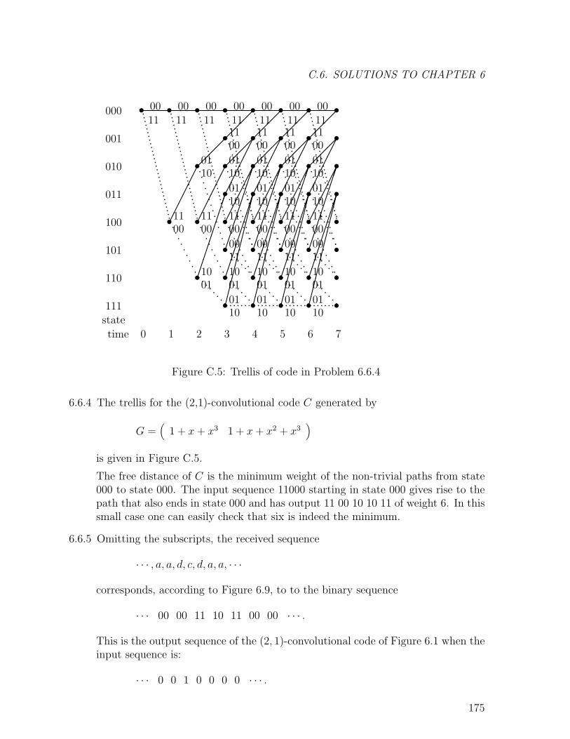
C.6. SOLUTIONS TO CHAPTER 6
• • • • • • • •
• • • • • •
• • • • • • •
• • • • • •
• • • • •
• • • • •
• • • • •
• • • • •
00 00 00 00 00 00 0011 11 11 11 11 11 11
11 11 11 11 11 1100 00 00 00 00 00
01 01 01 01 0110 10 10 10 10
10 10 10 10 1001 01 01 01 01
11 11 11 1100 00 00 00
01 01 01 0110 10 10 10
00 00 00 0011 11 11 11
01 01 01 0110 10 10 10
������
������
������
������
������
������
��
�
��
�
��
�
��
�
��
�
����������
����������
����������
����������
����������
��
�
��
�
��
�
��
�
������
������
������
������
����������
����������
����������
����������
������������
������������
������������
������������
·······························
·······························
·······························
·······························
·······························
·······························
·······························
···············
···············
···············
···············
···············
··········
··········
··········
··········
··········
··················
········
········
········
········
···············
···············
···············
···············
··········
··········
··········
··················
········
········
········
································
000
001
010
011
100
101
110
111state
time 0 1 2 3 4 5 6 7
Figure C.5: Trellis of code in Problem 6.6.4
6.6.4 The trellis for the (2,1)-convolutional code C generated by
G =(
1 + x+ x3 1 + x+ x2 + x3)
is given in Figure C.5.
The free distance of C is the minimum weight of the non-trivial paths from state000 to state 000. The input sequence 11000 starting in state 000 gives rise to thepath that also ends in state 000 and has output 11 00 10 10 11 of weight 6. In thissmall case one can easily check that six is indeed the minimum.
6.6.5 Omitting the subscripts, the received sequence
· · · , a, a, d, c, d, a, a, · · ·
corresponds, according to Figure 6.9, to to the binary sequence
· · · 00 00 11 10 11 00 00 · · · .
This is the output sequence of the (2, 1)-convolutional code of Figure 6.1 when theinput sequence is:
· · · 0 0 1 0 0 0 0 · · · .
175
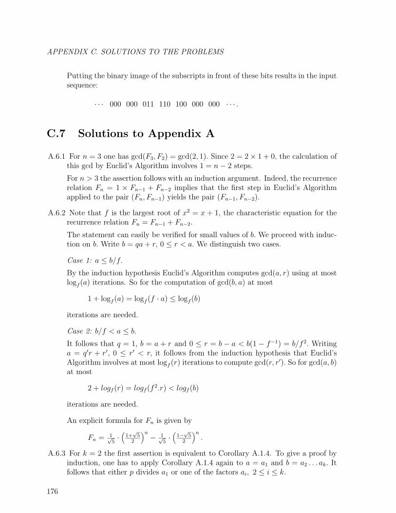
APPENDIX C. SOLUTIONS TO THE PROBLEMS
Putting the binary image of the subscripts in front of these bits results in the inputsequence:
· · · 000 000 011 110 100 000 000 · · · .
C.7 Solutions to Appendix A
A.6.1 For n = 3 one has gcd(F3, F2) = gcd(2, 1). Since 2 = 2× 1 + 0, the calculation ofthis gcd by Euclid’s Algorithm involves 1 = n− 2 steps.
For n > 3 the assertion follows with an induction argument. Indeed, the recurrencerelation Fn = 1 × Fn−1 + Fn−2 implies that the first step in Euclid’s Algorithmapplied to the pair (Fn, Fn−1) yields the pair (Fn−1, Fn−2).
A.6.2 Note that f is the largest root of x2 = x + 1, the characteristic equation for therecurrence relation Fn = Fn−1 + Fn−2.
The statement can easily be verified for small values of b. We proceed with induc-tion on b. Write b = qa+ r, 0 ≤ r < a. We distinguish two cases.
Case 1: a ≤ b/f.
By the induction hypothesis Euclid’s Algorithm computes gcd(a, r) using at mostlogf (a) iterations. So for the computation of gcd(b, a) at most
1 + logf (a) = logf (f · a) ≤ logf (b)
iterations are needed.
Case 2: b/f < a ≤ b.
It follows that q = 1, b = a + r and 0 ≤ r = b − a < b(1 − f−1) = b/f 2. Writinga = q′r + r′, 0 ≤ r′ < r, it follows from the induction hypothesis that Euclid’sAlgorithm involves at most logf (r) iterations to compute gcd(r, r′). So for gcd(a, b)at most
2 + logf (r) = logf (f2.r) < logf (b)
iterations are needed.
An explicit formula for Fn is given by
Fn = 1√5·(
1+√
52
)n− 1√
5·(
1−√
52
)n.
A.6.3 For k = 2 the first assertion is equivalent to Corollary A.1.4. To give a proof byinduction, one has to apply Corollary A.1.4 again to a = a1 and b = a2 . . . ak. Itfollows that either p divides a1 or one of the factors ai, 2 ≤ i ≤ k.
176
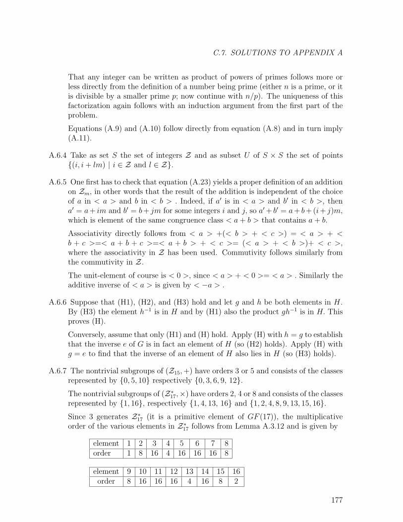
C.7. SOLUTIONS TO APPENDIX A
That any integer can be written as product of powers of primes follows more orless directly from the definition of a number being prime (either n is a prime, or itis divisible by a smaller prime p; now continue with n/p). The uniqueness of thisfactorization again follows with an induction argument from the first part of theproblem.
Equations (A.9) and (A.10) follow directly from equation (A.8) and in turn imply(A.11).
A.6.4 Take as set S the set of integers Z and as subset U of S × S the set of points{(i, i+ lm) | i ∈ Z and l ∈ Z}.
A.6.5 One first has to check that equation (A.23) yields a proper definition of an additionon Zm, in other words that the result of the addition is independent of the choiceof a in < a > and b in < b > . Indeed, if a′ is in < a > and b′ in < b >, thena′ = a+ im and b′ = b+ jm for some integers i and j, so a′ + b′ = a+ b+(i+ j)m,which is element of the same congruence class < a+ b > that contains a+ b.
Associativity directly follows from < a > +(< b > + < c >) = < a > + <b + c >=< a + b + c >=< a + b > + < c >= (< a > + < b >)+ < c >,where the associativity in Z has been used. Commutivity follows similarly fromthe commutivity in Z.The unit-element of course is < 0 >, since < a > + < 0 >= < a > . Similarly theadditive inverse of < a > is given by < −a > .
A.6.6 Suppose that (H1), (H2), and (H3) hold and let g and h be both elements in H.By (H3) the element h−1 is in H and by (H1) also the product gh−1 is in H. Thisproves (H).
Conversely, assume that only (H1) and (H) hold. Apply (H) with h = g to establishthat the inverse e of G is in fact an element of H (so (H2) holds). Apply (H) withg = e to find that the inverse of an element of H also lies in H (so (H3) holds).
A.6.7 The nontrivial subgroups of (Z15,+) have orders 3 or 5 and consists of the classesrepresented by {0, 5, 10} respectively {0, 3, 6, 9, 12}.The nontrivial subgroups of (Z∗
17,×) have orders 2, 4 or 8 and consists of the classesrepresented by {1, 16}, respectively {1, 4, 13, 16} and {1, 2, 4, 8, 9, 13, 15, 16}.Since 3 generates Z∗
17 (it is a primitive element of GF (17)), the multiplicativeorder of the various elements in Z∗
17 follows from Lemma A.3.12 and is given by
element 1 2 3 4 5 6 7 8order 1 8 16 4 16 16 16 8
element 9 10 11 12 13 14 15 16order 8 16 16 16 4 16 8 2
177
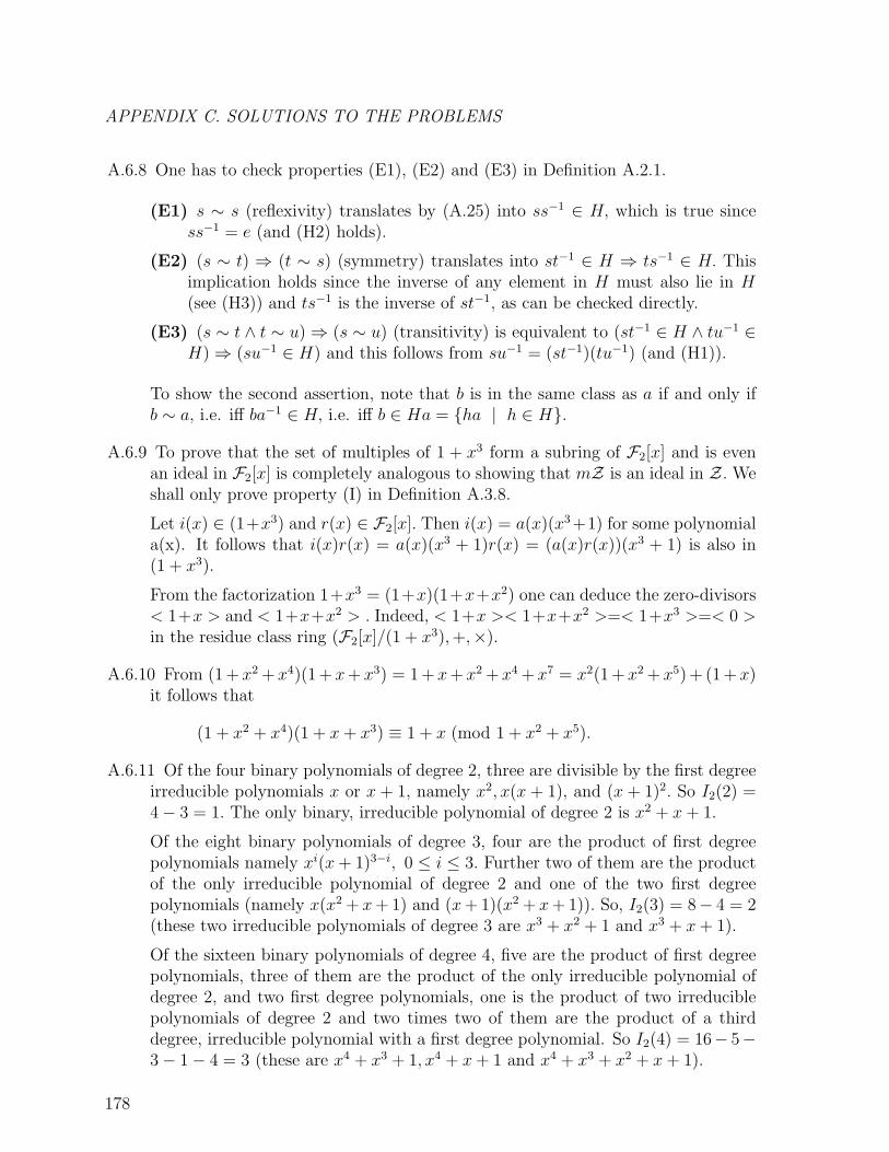
APPENDIX C. SOLUTIONS TO THE PROBLEMS
A.6.8 One has to check properties (E1), (E2) and (E3) in Definition A.2.1.
(E1) s ∼ s (reflexivity) translates by (A.25) into ss−1 ∈ H, which is true sincess−1 = e (and (H2) holds).
(E2) (s ∼ t) ⇒ (t ∼ s) (symmetry) translates into st−1 ∈ H ⇒ ts−1 ∈ H. Thisimplication holds since the inverse of any element in H must also lie in H(see (H3)) and ts−1 is the inverse of st−1, as can be checked directly.
(E3) (s ∼ t ∧ t ∼ u)⇒ (s ∼ u) (transitivity) is equivalent to (st−1 ∈ H ∧ tu−1 ∈H)⇒ (su−1 ∈ H) and this follows from su−1 = (st−1)(tu−1) (and (H1)).
To show the second assertion, note that b is in the same class as a if and only ifb ∼ a, i.e. iff ba−1 ∈ H, i.e. iff b ∈ Ha = {ha | h ∈ H}.
A.6.9 To prove that the set of multiples of 1 + x3 form a subring of F2[x] and is evenan ideal in F2[x] is completely analogous to showing that mZ is an ideal in Z. Weshall only prove property (I) in Definition A.3.8.
Let i(x) ∈ (1+x3) and r(x) ∈ F2[x]. Then i(x) = a(x)(x3+1) for some polynomiala(x). It follows that i(x)r(x) = a(x)(x3 + 1)r(x) = (a(x)r(x))(x3 + 1) is also in(1 + x3).
From the factorization 1+x3 = (1+x)(1+x+x2) one can deduce the zero-divisors< 1+x > and < 1+x+x2 > . Indeed, < 1+x >< 1+x+x2 >=< 1+x3 >=< 0 >in the residue class ring (F2[x]/(1 + x3),+,×).
A.6.10 From (1 + x2 + x4)(1 +x+ x3) = 1 + x+ x2 + x4 + x7 = x2(1 +x2 + x5) + (1 +x)it follows that
(1 + x2 + x4)(1 + x+ x3) ≡ 1 + x (mod 1 + x2 + x5).
A.6.11 Of the four binary polynomials of degree 2, three are divisible by the first degreeirreducible polynomials x or x + 1, namely x2, x(x + 1), and (x + 1)2. So I2(2) =4− 3 = 1. The only binary, irreducible polynomial of degree 2 is x2 + x+ 1.
Of the eight binary polynomials of degree 3, four are the product of first degreepolynomials namely xi(x+ 1)3−i, 0 ≤ i ≤ 3. Further two of them are the productof the only irreducible polynomial of degree 2 and one of the two first degreepolynomials (namely x(x2 + x+ 1) and (x+ 1)(x2 + x+ 1)). So, I2(3) = 8− 4 = 2(these two irreducible polynomials of degree 3 are x3 + x2 + 1 and x3 + x+ 1).
Of the sixteen binary polynomials of degree 4, five are the product of first degreepolynomials, three of them are the product of the only irreducible polynomial ofdegree 2, and two first degree polynomials, one is the product of two irreduciblepolynomials of degree 2 and two times two of them are the product of a thirddegree, irreducible polynomial with a first degree polynomial. So I2(4) = 16− 5−3− 1− 4 = 3 (these are x4 + x3 + 1, x4 + x+ 1 and x4 + x3 + x2 + x+ 1).
178
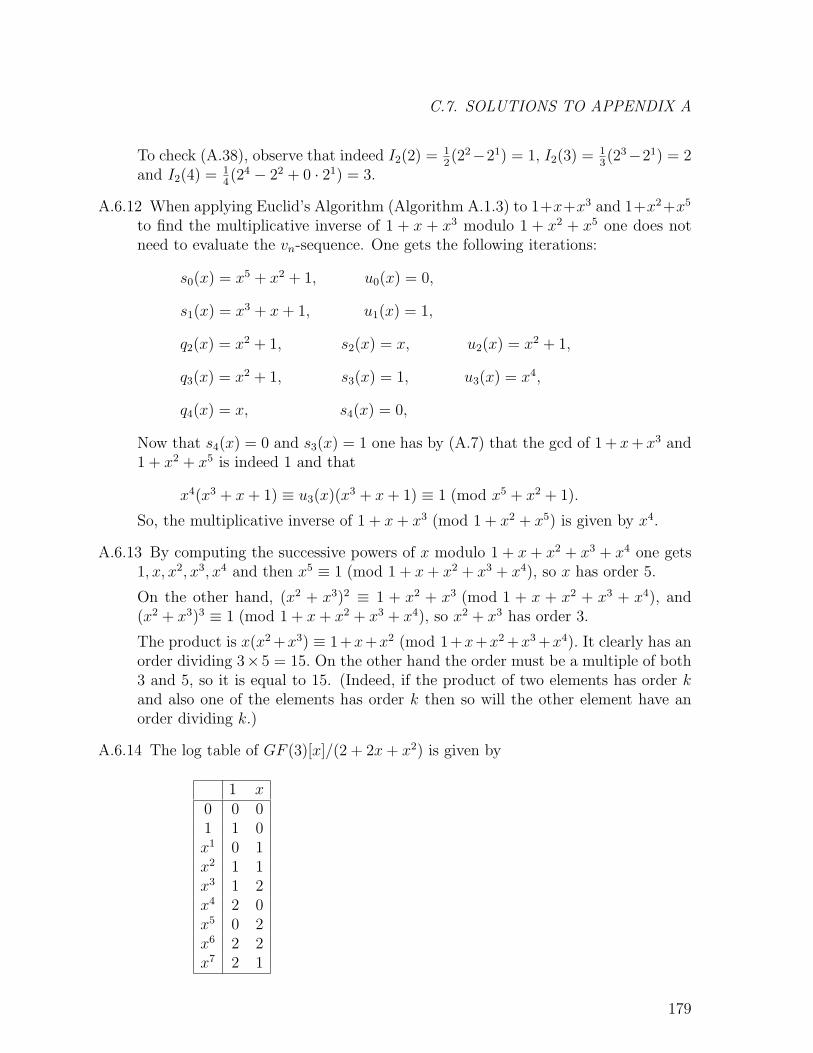
C.7. SOLUTIONS TO APPENDIX A
To check (A.38), observe that indeed I2(2) = 12(22−21) = 1, I2(3) = 1
3(23−21) = 2
and I2(4) = 14(24 − 22 + 0 · 21) = 3.
A.6.12 When applying Euclid’s Algorithm (Algorithm A.1.3) to 1+x+x3 and 1+x2+x5
to find the multiplicative inverse of 1 + x + x3 modulo 1 + x2 + x5 one does notneed to evaluate the vn-sequence. One gets the following iterations:
s0(x) = x5 + x2 + 1, u0(x) = 0,
s1(x) = x3 + x+ 1, u1(x) = 1,
q2(x) = x2 + 1, s2(x) = x, u2(x) = x2 + 1,
q3(x) = x2 + 1, s3(x) = 1, u3(x) = x4,
q4(x) = x, s4(x) = 0,
Now that s4(x) = 0 and s3(x) = 1 one has by (A.7) that the gcd of 1 + x+ x3 and1 + x2 + x5 is indeed 1 and that
x4(x3 + x+ 1) ≡ u3(x)(x3 + x+ 1) ≡ 1 (mod x5 + x2 + 1).
So, the multiplicative inverse of 1 + x+ x3 (mod 1 + x2 + x5) is given by x4.
A.6.13 By computing the successive powers of x modulo 1 + x + x2 + x3 + x4 one gets1, x, x2, x3, x4 and then x5 ≡ 1 (mod 1 + x+ x2 + x3 + x4), so x has order 5.
On the other hand, (x2 + x3)2 ≡ 1 + x2 + x3 (mod 1 + x + x2 + x3 + x4), and(x2 + x3)3 ≡ 1 (mod 1 + x+ x2 + x3 + x4), so x2 + x3 has order 3.
The product is x(x2 +x3) ≡ 1+x+x2 (mod 1+x+x2 +x3 +x4). It clearly has anorder dividing 3× 5 = 15. On the other hand the order must be a multiple of both3 and 5, so it is equal to 15. (Indeed, if the product of two elements has order kand also one of the elements has order k then so will the other element have anorder dividing k.)
A.6.14 The log table of GF (3)[x]/(2 + 2x+ x2) is given by
1 x0 0 01 1 0x1 0 1x2 1 1x3 1 2x4 2 0x5 0 2x6 2 2x7 2 1
179
APPENDIX C. SOLUTIONS TO THE PROBLEMS
A.6.15 The minimal polynomial of αi, i.e. mi(x), has as zeroes all the conjugates of αi.Since α has order 63, one gets
m1(x) has zeroes α1, α2, α4, α8, α16, α32;
m3(x) has zeroes α3, α6, α12, α24, α48, α96 = α33;
m9(x) has zeroes α9, α18, α36.
A.6.16 The multiplicative order of 3 modulo 11 is 5, since 35 ≡ 1 (mod 11) and nosmaller positive power of 3 has this property. It follows that α, a primitive 11-throot of unity in an extension field of GF (3), has the 5 conjugates: α, α3, α9, α27 =α5, α15 = α4.
The minimal polynomial of α is given by
(x− α)(x− α3)(x− α9)(x− α5)(x− α4).
and has degree 5.
A.6.17 By Corollary A.5.26, the field GF (625) = GF (54) contains as subfields GF (5m)with m|4, so GF (5) and GF (52).
The (ground)field GF (5) contains as elements the solutions of x5 = x, so 0 andthe fourth roots of unity ωi, 0 ≤ i ≤ 3, with ω = α(54−1)/(5−1) = α156.
The subfield GF (52) contains as elements the solutions of x25 = x, so 0 and the24-th roots of unity βi, 0 ≤ i ≤ 23, with β = α(54−1)/(52−1) = α26.
A.6.18 Let α be a primitive 17-th root of unity. Its conjugates are
α, α2, α4, α8, α16, α15, α13, α9.
It follows that m1(x), the minimal polynomial of α, has degree 8.
The minimal polynomial m3(x) of α3 has zeroes
α3, α6, α12, α7, α14, α11, α5, α10.
We conclude that the two different minimal polynomials of primitive 17-th rootsof unity are m1(x) and m3(x). Of course
x17 − 1 = (x− 1)m1(x)m3(x).
From
x8m1(x−1) = x8∏7
i=0(x−1 − α2i
) =∏7
i=0(1− α2ix)
= α1+2+4+8+16+15+13+9∏7i=0(α
−2i − x)
=∏7
i=0(x− α−2i) =
∏7i=0(x− α2i
) = m1(x).
180
C.7. SOLUTIONS TO APPENDIX A
It follows that m1(x) is its own reciprocal. The same holds for m3(x).
So, we can write m1(x) and m3(x) as follows:
m1(x) = 1 + ax+ bx2 + cx3 + dx4 + cx5 + bx6 + ax7 + x8,
m3(x) = 1 + sx+ tx2 + ux3 + vx4 + ux5 + tx6 + sx7 + x8.
Since m1(x)m3(x) = (x17−1)/(x−1) = 1+x+x2 + . . .+x16, we get the followingequations:
(x): a+ s = 1,(x2): t+ as+ b = 1,(x3): u+ at+ bs+ c = 1,(x4): v + au+ bt+ cs+ d = 1,(x5): u+ av + bu+ ct+ ds+ c = 1,(x6): t+ au+ bv + cu+ dt+ cs+ b = 1,(x7): s+ at+ bu+ cv + du+ ct+ bs+ a = 1,(x8): dv = 1,
From (x8) we conclude that d = v = 1. Now, without loss of generality, (x) yieldsa = 1 and s = 0 (otherwise, interchange the role of m1(x) and m3(x), i.e. take α3
as primitive 17-th root of unity).
Substituting these values in (x2) yields t + b = 1 and thus tb = 0. Equation (x4)now reduces to u = 1 and (x3) to t = c. Next, (x5) yields (since tc = cc = c) b = 1.Finally, (x2) gives t = 0 and (x3) gives t = c.
Summarizing, one has obtained
m1(x) = 1 + x+ x2 + x4 + x6 + x7 + x8,
m3(x) = 1 + x3 + x4 + x5 + x8.
A.6.19 We use the same numbering as in the problem.
1. It follows from Corollary A.5.13 and Corollary A.5.4 that
(Tr(x))p = (x+ xp + xp2+ · · ·+ xpm−2
+ xpm−1)p =
= (xp + xp2+ xp3
+ · · ·+ xpm−1+ x) = Tr(x).
Theorem A.5.14 now implies that Tr(x) ∈ GF (p) for all x ∈ GF (pm).
2. Let x and y be elements in GF (q) and a and b in GF (p). Then, by CorollaryA.5.13 and Theorem A.5.14,
Tr(ax+ by) =
= (ax+ by) + (ax+ by)p + · · ·+ (ax+ by)pm−1
181
APPENDIX C. SOLUTIONS TO THE PROBLEMS
= (ax+ by) + (apxp + bpyp) + · · ·+ (apm−1xpm−1
+
+bpm−1
ypm−1)
= (ax+ by) + (axp + byp) + · · ·+ (axpm−1+ bypm−1
)
= a(x+ xp + · · ·+ xpm−1) + b(y + yp + · · ·+ ypm−1
)
= aTr(x) + bTr(y).
This proves the linearity of the trace mapping.
3. Since Tr(x) is a linear mapping fromGF (pm) toGF (p), it either is the all-zeromapping or it takes on every value in GF (p) equally often. However, Tr(x)is a polynomial of degree pm−1, so it has at most pm−1 zeroes by TheoremA.4.14. Consequently, Tr(x) is not identical to zero and thus it takes on everyvalue in GF (p) equally often.
182
Bibliography
[1] Arazi, B., A commonsense approach to the theory of error correcting codes, MITPress Series in Computer Systems, Cambridge MA, 1988.
[2] Beker, H.J. and F.C. Piper, Cryptography and coding, Clarendon Press, Oxford,Great. Britt., 1989.
[3] Berlekamp E.R., Algebraic coding theory, Revised 1984 edition, Aegean Park Press,1984.
[4] Berlekamp E.R., Key Papers in the Development of Coding Theory, IEEE PressSelected Reprint Series, New York, 1974.
[5] Blahut, R.E., Theory and practice of error control codes, (reprint), Addison-WesleyPublishing Company, Reading MA, 1984.
[6] Blake, I.F., Algebraic coding theory, Benchmark Papers in Electrical Engineeringand Computer Science, Hutchinson & Ross, Inc., Dowden, 1973.
[7] Blake, I.F. and R. Mullin, The mathematical theory of coding, Academic Press, NewYork, 1975.
[8] Cameron, P.J. and J.H. van Lint, Designs, graphs, codes and their links, LondonMathematical Society Student Texts 22, Cambridge University Press, Cambridge,1991.
[9] Chambers, W.G., Basics of communications and coding, Clarendon Press, Oxford,Great. Britt., 1985.
[10] Clark, Jr., G.C. and J.B. Cain, Error-correction coding for digital communications,Plenum Press, New York etc., 1981.
[11] Gallager, R.G., Information theory and reliable communication, Wiley, New York,1968.
[12] Hamming, R.W., Coding and information theory, Prentice-Hall, Inc., EnglewoodCliffs, N.J., 1980.
183
CODING THEORY
[13] Hill, R., A first course in coding theory, Clarendon Press, Oxford, Great. Britt.,1986.
[14] Lin, S. and D.J. Costello, Jr., Error control coding; fundamentals and applications,Prentice-Hall, Inc., Englewood Cliffs, N.J., 1983.
[15] Lint, J.H. van, Coding theory, Springer Lecture Notes, Vol. 201, Springer Verlag,Berlin etc., 1971.
[16] Lint, J.H. van, Introduction to coding theory, Graduate Texts in Mathematics, Vol.86, Springer-Verlag, New York etc., 1982; second edition 1992.
[17] Lint, J.H. van, and G. van der Geer, Introduction to coding theory and algebraicgeometry, Birkhauser, Basel, 1988.
[18] MacWilliams, F.J. and N.J.A. Sloane, The theory of error-correcting codes, NorthHolland, Amsterdam etc., 1977.
[19] McEliece, R.J., The theory of information and coding, Encyclopedia of Math. and itsApplications, Vol. 3, Addison-Wesley Publishing Company, Reading, Mass., 1977.
[20] Moreno, C.J., Algebraic curves over finite fields, Cambridge University Press, Cam-bridge etc., 1991.
[21] Peterson, W.W. and E.J. Weldon, Error-correcting codes (2nd ed.), MIT Press,Cambridge, Mass., 1972.
[22] Pless, V., Introduction to the theory of error-correcting codes (2nd ed.), John Wileyand Sons, New York etc., 1989.
[23] Pretzel, O., Error-correcting codes and finite fields, Clarendon Press, Oxford, Great.Britt., 1992.
[24] Rao, T.R.N. and E. Fujiwara, Error-control coding for computer systems, Prentice-Hall Series in Computer Engineering, Prentice-Hall, Inc., Englewood Cliffs, N.J.,1989.
[25] Rhee, M.Y., Error-correcting coding theory, McGraw–Hill Publishing Company,New York, 1989.
[26] Sweeney, P., Error control coding: an introduction, Prentice Hall, New York, 1991.
[27] Thompson, T.M., From error-correcting codes through sphere packings to simplegroups, Mathematical Association of America, Providence R.I., 1983.
[28] Tsfasman, M.A. and S.G. Vladut, Algebraic-geometric codes, Kluwer Academic Pub-lishers, Dordrecht, 1991.
184

BIBLIOGRAPHY
[29] Vanstone, S.A. and P.C. van Oorschot, An introduction to error correcting codeswith applications, Kluwer Academic Publishers, Boston MA, 1989.
[30] Welsh, D., Codes and cryptography, Clarendon Press, Oxford, Great. Britt., 1988.
185
Index
Abramson bound, 105AES-conditions, 121affine line, 83AG code, 82AG-code, 82algebraic curve, 82algebraic-geometry code, 82algorithm
Euclid’s, 146array code, 112associative, 152automorphism, 48
b-burst-correcting code, 103bandpass Gaussian channel, 138basic algorithm, 96basis, 168BCH bound, 66BCH code, 66binary symmetric channel, 2block code, 6, 11bounds
Abramson, 105BCH, 66Gilbert-Varshamov, 15Griesmer, 39Hamming, 13Reiger, 104Singleton, 15sphere packing, 14
BSC, 2burst, 3, 103burst pattern, 103burst start, 103burst-channel, 3burst-correcting code, 103
candidate, 90capacity, 8catastrophic, 128channel, 2
bandpass Gaussian, 138binary symmetric, 2BSC, 2burst, 3error and erasure, 3Gaussian, 3q-ary symmetric, 3
character, 23characteristic, 166characteristic vector, 45class
congruence, 151equivalence, 151
codesAG, 82algebraic-geometry, 82array, 112BCH, 66block, 6, 11burst-correcting, 103concatenated, 40convolutional, 6, 125cyclic, 55cyclic b-burst-correcting, 105dual, 19equivalent, 14even weight, 17extended, 37Fire, 108geometric Goppa, 82Golay, binary, 69
186
INDEX
Golay, ternary, 70Goppa, 72Hamming, 41inner, 40linear, 16linear unequal error protection, 28LUEP, 28maximum distance separable, 15MDS, 15narrow-s ense BCH, 66optimum, cyclic, b-burst-correcting,
105outer, 40perfect, 13primitive BCH, 66projective, 41punctured, 38Reed-Muller, 45Reed-Solomon, 68repetition, 14residual, 38RM, 45self-dual, 19self-orthogonal, 19shortened, 38Simplex, 43trivial, 12
codeword, 6, 11, 125coefficient, 159communication system, 5commutative, 152commutative field, 156commutative group, 153commutative ring, 155complete, 5concatenated code, 40congruence class, 151congruence relation, 149congruent, 149conjugate, 61, 171constellation, 138constraint length, 125convolutional code, 6, 125
correct candidate, 90coset, 20coset leader, 20covering radius, 13cyclic, 55cyclic b-burst-correcting code, 105cyclic burst, 105cyclic group, 156cyclotomic coset, 61
decoder, 5decoding algorithms
algebraic geometry code, 93array, 116BCH, 74BCH, binary, 80BCH, binary, e=2, 65complete, 5Fire, 110geometric Goppa code, 93Goppa, 79Goppa, binary, 82hard decision, 5incomplete, 5majority-logic, 51maximum likelihood, 5multi-step, 51optimum, cyclic 2-burst-correcting, 119Reed Solomon, 74soft decision, 5syndrome decoding, 20Viterbi, 132
defining set, 61degree, 44, 87, 159, 172
of a monomial, 87of a polynomial, 44of a syndrome, 87, 88
demodulator, 138depth, 106designed distance, 66discrepancy, 90distance
free, 130
187
CODING THEORY
Hamming, 11divide, 145dual code, 19
elliptic curve, 84encoder, 5entropy function, 7equivalence class, 151equivalence relation, 151equivalent, 14erasure, 3erasure correction, 12error, 2error and erasure channel, 3error evaluator polynomial, 75error location, 75error locator polynomial, 75error value, 75error-correction, 12error-detection, 12Euclid’s Algorithm, 76Euclid’s algorithm, 146Euler’s Totient Function, 148even weight code, 17extended, 37extension field, 168
Fibonacci numbers, 175field, 155
commutative, 156extension, 168finite, 156Galois, 156ground, 168sub–, 156
finite, 156Fire code, 108first error probability,, 136Fourier transform, 88free distance, 130function, 82fundamental path, 134fundamental path enumerator, 135
Galois field, 156gap, 109Gaussian channel, 3gcd, 146generate, 156, 160generator matrix, 17, 125generator polynomial, 57geometric Goppa code, 82Gilbert-Varshamov bound, 15Golay code, binary, 69Golay code, ternary, 70Goppa code, 72greatest common divisor, 146Griesmer bound, 39ground field, 168group, 153
commutative, 153cyclic, 156finite, 156sub–, 154
Hamming bound, 13Hamming code, 41Hamming distance, 11Hamming weight, 16hard decision, 5
ideal, 155idempotent, 99incomplete, 5incorrect candidate, 90information rate, 6information symbol, 18information vector, 17inner code, 40interleaving, 106invariant factors, 126inverse, 153invertible, 125irreducible, 159isomorphic, 167
key equation, 75
lcm, 146
188

INDEX
least common multiple, 146length, 11, 103linear code, 16linear congruence relation, 150linear unequal error protection code, 28log table, 166LUEP code, 28
MacWilliams relations, 24majority-logic decoding, 51Mattson-Solomon polynomial, 67maximum distance separable code, 15maximum likelihood decoder, 5MDS code, 15message vector, 17minimal polynomial, 62, 172minimum distance, 12Mobius function, 162Mobius Inversion Formula, 163modulator, 138modulo, 149, 158monic, 161multi-step, 51
narrow-sense, 66
operation, 152optimal generator matrix, 29optimum, cyclic, b-burst-correcting code,
105order, 156orthogonal, 19outer code, 40
p-ary, 160parity check matrix, 18parity check polynomial, 59parity check symbol, 19path enumerator, 135perfect, 13period, 108point, 82polynomial, 159
error evaluator, 75
error locator, 75generator, 57Mattson-Solomon, 67minimal, 62, 172monic, 161parity check, 59primitive, 60, 172
primitive n-th root of unity, 61, 164primitive BCH code, 66primitive element, 60, 164primitive polynomial, 60, 172principal character, 23principal ideal ring, 160projective code, 41puncturing, 38
q-ary symmetric channel, 3
rate, 14, 125receiver, 1reducible, 159redundancy, 4, 18Reed-Muller code, 45Reed-Solomon code, 68Reiger bound, 104relation, 151
congruence, 149equivalence, 151linear congruence, 150
repetition code, 14residual code, 38residue class ring, 158ring, 154
commutative, 155finite, 156principal ideal, 160residue class, 158sub–, 155
RM, 45root of unity, 164
self-dual, 19self-orthogonal, 19sender, 1
189
CODING THEORY
separation vector, 27, 29shortening, 38Simplex code, 43Singleton bound, 15sink, 1soft decision, 5source, 1sphere, 12sphere packing bound, 14standard form, 18state, 125subfield, 156subgroup, 154subring, 155survivor, 131syndrome, 20
first order, 87second order, 88
syndrome decoding algorithm, 20systematic, 18
trace, 24, 177trellis, 129trivial code, 12
unique, 70unit-element, 152
Viterbi decoding algorithm, 132
weight, 16, 131weight enumerator, 23
zero-divisor, 156
190