Embed Size (px)
Citation preview

Coding Theory and
Projective Spaces
Natalia Silberstein
Technion - Computer Science Department - Ph.D. Thesis PHD-2011-13 - 2011

Technion - Computer Science Department - Ph.D. Thesis PHD-2011-13 - 2011

Coding Theory and
Projective Spaces
Research Thesis
In Partial Fulfillment of the Requirements for the
Degree of Doctor of Philosophy
Natalia Silberstein
Submitted to the Senate of
the Technion — Israel Institute of Technology
Elul 5771 Haifa September 2011
Technion - Computer Science Department - Ph.D. Thesis PHD-2011-13 - 2011

Technion - Computer Science Department - Ph.D. Thesis PHD-2011-13 - 2011

This Research Thesis was done under the supervision of Prof. Tuvi Etzion in the
Department of Computer Science.
I wish to express my sincere and deepest gratitude to my supervisor Prof. Tuvi Etzion
for his thoughtful and patient guidance, and for all the encouragement and support he
provided throughout the ups and downs of this research.
I thank my family, and in particular, my parents Tatyana and Michael Turich. Their
love and belief in my success, as well as their ”never-give-up” principle which they followed
themselves and imprinted in me, were instrumental to all my achievements. I owe my
greatest gratitude to my parents-in-law, Alla and Boris Silberstein, for their unconditional
and loving help. But above all, I want to thank my two beloved sons Danny and Benny
and my husband Mark for their endless love, understanding and patience.
I dedicate this work in memory of my dearest mother.
The Generous Financial Help Of The Technion, Israeli Science Foundation, and Neaman
Foundation Is Gratefully Acknowledged
Technion - Computer Science Department - Ph.D. Thesis PHD-2011-13 - 2011

Technion - Computer Science Department - Ph.D. Thesis PHD-2011-13 - 2011
List of Publications
Journal Publications
1. T. Etzion and N. Silberstein, “Error-Correcting Codes in Projective Spaces Via
Rank-Metric Codes and Ferrers Diagrams”, IEEE Transactions on Information The-
ory, Vol. 55, No. 7, pp. 2909–2919, July 2009.
2. N. Silberstein and T. Etzion, “Enumerative Coding for Grassmannian Space”, IEEE
Transactions on Information Theory, Vol. 57, No. 1, pp. 365 - 374, January 2011.
3. N. Silberstein and T. Etzion, “Large Constant Dimension Codes and Lexicodes”,
Advances in Mathematics of Communications (AMC), vol. 5, No. 2, pp. 177 - 189,
2011.
4. T. Etzion and N. Silberstein, “Codes and Designs Related to Lifted MRD Codes”,
submitted to IEEE Transactions on Information Theory.
Conference Publications
1. T. Etzion and N. Silberstein, “Construction of Error-Correcting Codes For Random
Network Coding”, in IEEE 25th Convention of Electrical & Electronics Engineers in
Israel (IEEEI 2008), pp. 70 - 74, Eilat, Israel, December 2008.
2. N. Silberstein and T. Etzion, “Enumerative Encoding in the Grassmannian Space”,
in 2009 IEEE Information Theory Workshop (ITW 2009), pp. 544 - 548, Taormina,
Sicily, October 2009.
3. N. Silberstein and T. Etzion, “Large Constant Dimension Codes and Lexicodes”,
in Algebraic Combinatorics and Applications (ALCOMA 10), Thurnau, Germany,
April 2010.
4. N. Silberstein and T. Etzion, “Codes and Designs Related to Lifted MRD Codes”,
in IEEE International Symposium on Information Theory (ISIT 2011), pp. 2199 -
2203, Saint Petersburg, Russia, July-August 2011.
Technion - Computer Science Department - Ph.D. Thesis PHD-2011-13 - 2011

Technion - Computer Science Department - Ph.D. Thesis PHD-2011-13 - 2011

Contents
Abstract 1
Abbreviations and Notations 3
1 Introduction 5
1.1 Codes in Projective Space . . . . . . . . . . . . . . . . . . . . . . . . . . . . 5
1.2 Random Network Coding . . . . . . . . . . . . . . . . . . . . . . . . . . . . 6
1.2.1 Errors and Erasures Correction in Random Network Coding . . . . . 6
1.3 Rank-Metric Codes . . . . . . . . . . . . . . . . . . . . . . . . . . . . . . . . 8
1.4 Related Work . . . . . . . . . . . . . . . . . . . . . . . . . . . . . . . . . . . 9
1.4.1 Bounds . . . . . . . . . . . . . . . . . . . . . . . . . . . . . . . . . . 9
1.4.2 Constructions of Codes . . . . . . . . . . . . . . . . . . . . . . . . . 12
1.5 Organization of This Work . . . . . . . . . . . . . . . . . . . . . . . . . . . 14
2 Representations of Subspaces and Distance Computation 16
2.1 Representations of Subspaces . . . . . . . . . . . . . . . . . . . . . . . . . . 16
2.1.1 Reduced Row Echelon Form Representation . . . . . . . . . . . . . . 16
2.1.2 Ferrers Tableaux Form Representation . . . . . . . . . . . . . . . . . 18
2.1.3 Extended Representation . . . . . . . . . . . . . . . . . . . . . . . . 21
2.2 Distance Computation . . . . . . . . . . . . . . . . . . . . . . . . . . . . . . 22
3 Codes and Designs Related to Lifted MRD Codes 26
3.1 Lifted MRD Codes and Transversal Designs . . . . . . . . . . . . . . . . . . 27
3.1.1 Properties of Lifted MRD Codes . . . . . . . . . . . . . . . . . . . . 27
3.1.2 Transversal Designs from Lifted MRD Codes . . . . . . . . . . . . . 30
3.2 Linear Codes Derived from Lifted MRD Codes . . . . . . . . . . . . . . . . 32
i
Technion - Computer Science Department - Ph.D. Thesis PHD-2011-13 - 2011

3.2.1 Parameters of Linear Codes Derived from CMRD . . . . . . . . . . . 33
3.2.2 LDPC Codes Derived from CMRD . . . . . . . . . . . . . . . . . . . 39
4 New Bounds and Constructions for Codes in Projective Space 43
4.1 Multilevel Construction via Ferrers Diagrams Rank-Metric Codes . . . . . . 43
4.1.1 Ferrers Diagram Rank-Metric Codes . . . . . . . . . . . . . . . . . . 44
4.1.2 Lifted Ferrers Diagram Rank-Metric Codes . . . . . . . . . . . . . . 49
4.1.3 Multilevel Construction . . . . . . . . . . . . . . . . . . . . . . . . . 51
4.1.4 Code Parameters . . . . . . . . . . . . . . . . . . . . . . . . . . . . . 53
4.1.5 Decoding . . . . . . . . . . . . . . . . . . . . . . . . . . . . . . . . . 54
4.2 Bounds and Constructions for Constant Dimension Codes that Contain CMRD 56
4.2.1 Upper Bounds for Constant Dimension Codes . . . . . . . . . . . . . 57
4.2.2 Upper Bounds for Codes which Contain Lifted MRD Codes . . . . . 59
4.2.3 Construction for (n,M, 4, 3)q Codes . . . . . . . . . . . . . . . . . . 61
4.2.4 Construction for (8,M, 4, 4)q Codes . . . . . . . . . . . . . . . . . . 66
4.3 Error-Correcting Projective Space Codes . . . . . . . . . . . . . . . . . . . . 69
4.3.1 Punctured Codes . . . . . . . . . . . . . . . . . . . . . . . . . . . . . 70
4.3.2 Code Parameters . . . . . . . . . . . . . . . . . . . . . . . . . . . . . 72
4.3.3 Decoding . . . . . . . . . . . . . . . . . . . . . . . . . . . . . . . . . 73
5 Enumerative Coding and Lexicodes in Grassmannian 76
5.1 Lexicographic Order for Grassmannian . . . . . . . . . . . . . . . . . . . . . 77
5.1.1 Order for Gq(n, k) Based on Extended Representation . . . . . . . . 77
5.1.2 Order for Gq(n, k) Based on Ferrers Tableaux Form . . . . . . . . . . 78
5.2 Enumerative Coding for Grassmannian . . . . . . . . . . . . . . . . . . . . . 79
5.2.1 Enumerative Coding for Gq(n, k) Based on Extended Representation 80
5.2.2 Enumerative Coding for Gq(n, k) Based on Ferrers Tableaux Form . 87
5.2.3 Combination of the Coding Techniques . . . . . . . . . . . . . . . . 94
5.3 Constant Dimension Lexicodes . . . . . . . . . . . . . . . . . . . . . . . . . 97
5.3.1 Analysis of Constant Dimension Codes . . . . . . . . . . . . . . . . . 97
5.3.2 Search for Constant Dimension Lexicodes . . . . . . . . . . . . . . . 101
6 Conclusion and Open Problems 106
Bibliography 108
ii
Technion - Computer Science Department - Ph.D. Thesis PHD-2011-13 - 2011

List of Figures
1.1 Network coding example. Max-flow is attainable only through the mixing
of information at intermediate nodes. . . . . . . . . . . . . . . . . . . . . . . 7
iii
Technion - Computer Science Department - Ph.D. Thesis PHD-2011-13 - 2011

List of Tables
3.1 LDPC codes from CMRD vs. LDPC codes from finite geometries . . . . . . 40
4.1 The (8, 4573, 4, 4)2 code C . . . . . . . . . . . . . . . . . . . . . . . . . . . . 53
4.2 CML vs. CMRD . . . . . . . . . . . . . . . . . . . . . . . . . . . . . . . . . . 54
4.3 Qs(q) . . . . . . . . . . . . . . . . . . . . . . . . . . . . . . . . . . . . . . . 58
4.4 Q′δ−1(q) for k = 3 . . . . . . . . . . . . . . . . . . . . . . . . . . . . . . . . 58
4.5 Q′δ−1(q) for k = 4 . . . . . . . . . . . . . . . . . . . . . . . . . . . . . . . . 58
4.6 Lower bound on |CML|upper bound . . . . . . . . . . . . . . . . . . . . . . . . . . . 59
4.7 The size of new codes vs. the previously known codes and the upper
bound (4.3) . . . . . . . . . . . . . . . . . . . . . . . . . . . . . . . . . . . . 66
4.8 Lower bounds on ratio between |Cnew| and the bound in (4.3) . . . . . . . 66
4.9 The size of new codes vs. previously known codes and bound (4.3) . . . . . 68
4.10 The punctured (7, 573, 3)q code C′Q,v . . . . . . . . . . . . . . . . . . . . . . 71
5.1 Clex vs. CML in G2(8, 4) with dS = 4 . . . . . . . . . . . . . . . . . . . . . . 102
iv
Technion - Computer Science Department - Ph.D. Thesis PHD-2011-13 - 2011

Abstract
The projective space of order n over a finite field Fq, denoted by Pq(n), is a set of all
subspaces of the vector space Fnq . The projective space is a metric space with the distance
function ds(X,Y ) = dim(X)+dim(Y )−2dim(X ∩Y ), for all X,Y ∈ Pq(n). A code in the
projective space is a subset of Pq(n). Coding in the projective space has received recently
a lot of attention due to its application in random network coding.
If the dimension of each codeword is restricted to a fixed nonnegative integer k ≤ n,
then the code forms a subset of a Grassmannian, which is the set of all k-dimensional
subspaces of Fnq , denoted by Gq(n, k). Such a code is called a constant dimension code.
Constant dimension codes in the projective space are analogous to constant weight codes
in the Hamming space.
In this work, we consider error-correcting codes in the projective space, focusing mainly
on constant dimension codes.
We start with the different representations of subspaces in Pq(n). These representa-
tions involve matrices in reduced row echelon form, associated binary vectors, and Ferrers
diagrams. Based on these representations, we provide a new formula for the computation
of the distance between any two subspaces in the projective space.
We examine lifted maximum rank distance (MRD) codes, which are nearly optimal
constant dimension codes. We prove that a lifted MRD code can be represented in such
a way that it forms a block design known as a transversal design. A slightly different
representation of this design makes it similar to a q-analog of transversal design. The
incidence matrix of the transversal design derived from a lifted MRD code can be viewed
as a parity-check matrix of a linear code in the Hamming space. We find the properties
of these codes which can be viewed also as LDPC codes.
We present new bounds and constructions for constant dimension codes. First, we
present a multilevel construction for constant dimension codes, which can be viewed as a
1
Technion - Computer Science Department - Ph.D. Thesis PHD-2011-13 - 2011

generalization of a lifted MRD codes construction. This construction is based on a new
type of rank-metric codes, called Ferrers diagram rank-metric codes. We provide an upper
bound on the size of Ferrers diagram rank-metric codes and present a construction of codes
that attain this bound. Then we derive upper bounds on the size of constant dimension
codes which contain the lifted MRD code, and provide a construction for two families of
codes, that attain these upper bounds. Most of the codes obtained by these constructions
are the largest known constant dimension codes. We generalize the well-known concept of
a punctured code for a code in the projective space to obtain large codes which are not
constant dimension.
We present efficient enumerative encoding and decoding techniques for the Grassman-
nian. These coding techniques are based on two different lexicographic orders for the
Grassmannian induced by different representations of k-dimensional subspaces of Fnq . Fi-
nally we describe a search method for constant dimension lexicodes. Some of the codes
obtained by this search are the largest known constant dimension codes with their param-
eters.
2
Technion - Computer Science Department - Ph.D. Thesis PHD-2011-13 - 2011

Abbreviations and Notations
Fq — a finite field of size q
Pq(n) — the projective space of order n
Gq(n, k) — the Grassmannian
dS(·, ·) — the subspace distance
dR(·, ·) — the rank distance
dH(·, ·) — the Hamming distance
C — a code in the projective space
CMRD — the lifted MRD code
C — a rank-metric code
C — a code in the Hamming space
RREF — reduced row echelon form
RE(X) — a subspace X in RREF
v(X) — the identifying vector of a subspace X
FE(X) — the Ferrers echelon form of a subspace X
F — Ferrers diagram
FX — the Ferrers diagram of a subspace X
F(X) — the Ferrers taubleux form of a subspace X
EXT(X) — the extended representation of a subspace X[n
k
]q
— the q-ary Gaussian coefficient
TDλ(t, k,m) — a transversal design of blocksize k, groupsize m,
strength t and index λ
TDλ(k,m) — a transversal design TDλ(2, k,m)
STDq(t, k,m) — a subspace transversal design of block dimension k,
groupsize qm and strength t
OAλ(N, k, s, t) — an N × k orthogonal array with s levels, strength t, and index λ
3
Technion - Computer Science Department - Ph.D. Thesis PHD-2011-13 - 2011

4
Technion - Computer Science Department - Ph.D. Thesis PHD-2011-13 - 2011
Chapter 1
Introduction
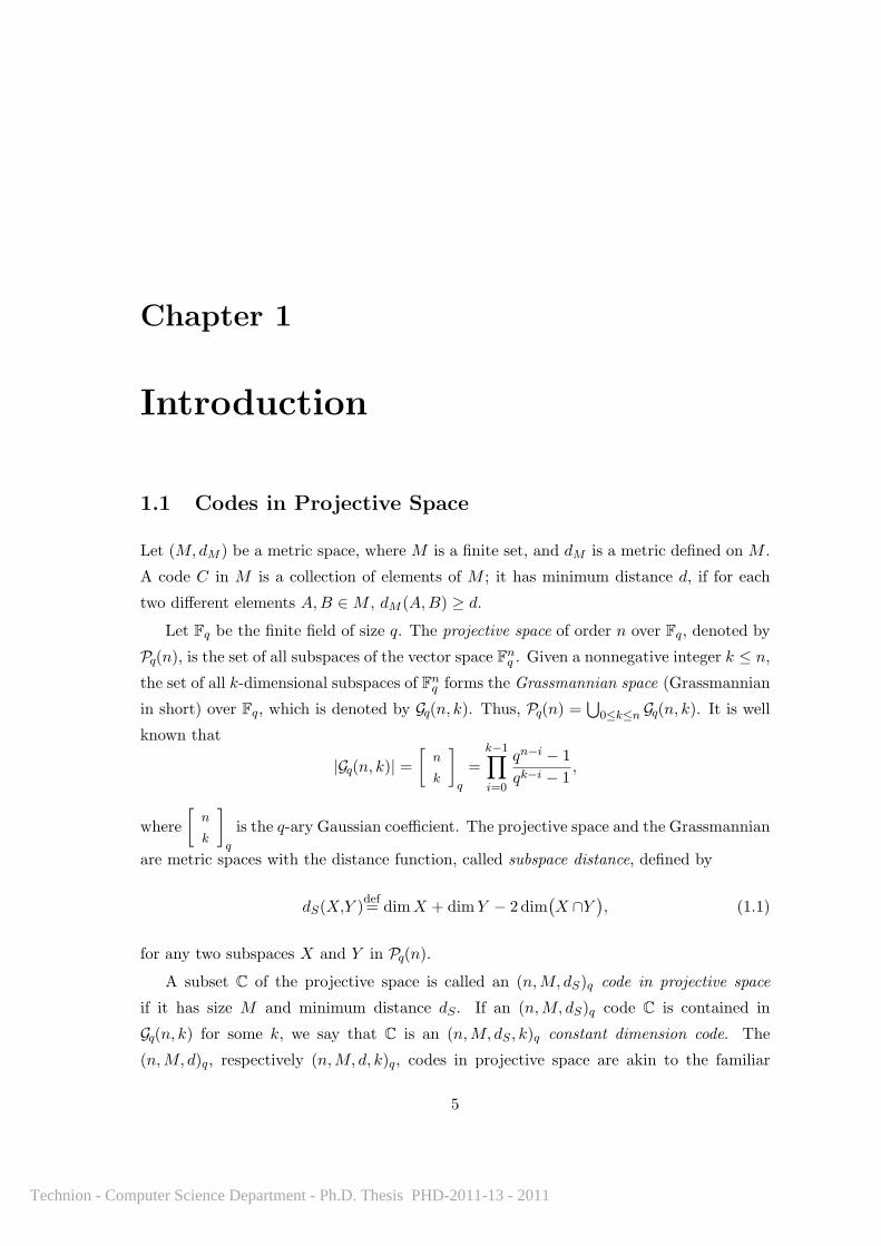
1.1 Codes in Projective Space
Let (M,dM ) be a metric space, where M is a finite set, and dM is a metric defined on M .
A code C in M is a collection of elements of M ; it has minimum distance d, if for each
two different elements A,B ∈ M , dM (A,B) ≥ d.
Let Fq be the finite field of size q. The projective space of order n over Fq, denoted by
Pq(n), is the set of all subspaces of the vector space Fnq . Given a nonnegative integer k ≤ n,
the set of all k-dimensional subspaces of Fnq forms the Grassmannian space (Grassmannian
in short) over Fq, which is denoted by Gq(n, k). Thus, Pq(n) =∪
0≤k≤n Gq(n, k). It is well
known that
|Gq(n, k)| =[
n
k
]q
=k−1∏i=0
qn−i − 1
qk−i − 1,
where
[n
k
]q
is the q-ary Gaussian coefficient. The projective space and the Grassmannian
are metric spaces with the distance function, called subspace distance, defined by
dS(X,Y )def= dimX + dimY − 2 dim
(X ∩Y
), (1.1)
for any two subspaces X and Y in Pq(n).
A subset C of the projective space is called an (n,M, dS)q code in projective space
if it has size M and minimum distance dS . If an (n,M, dS)q code C is contained in
Gq(n, k) for some k, we say that C is an (n,M, dS , k)q constant dimension code. The
(n,M, d)q, respectively (n,M, d, k)q, codes in projective space are akin to the familiar
5
Technion - Computer Science Department - Ph.D. Thesis PHD-2011-13 - 2011

codes in the Hamming space, respectively constant-weight codes in the Johnson space,
where the Hamming distance serves as the metric.
Koetter and Kschischang [43] showed that codes in Pq(n) are precisely what is needed
for error-correction in random network coding [11, 12]. This is the motivation to explore
error-correcting codes in Pq(n).
1.2 Random Network Coding
A network is a directed graph, where the edges represent pathways for information. Using
the max-flow min-cut theorem, one can calculate the maximum amount of information
that can be pushed through this network between any two graph nodes. It was shown
that simple forwarding of information between the nodes is not capable of attaining the
max-flow value. Rather, by allowing mixing of data at intermediate network nodes this
value can be achieved. Such encoding is referred to as network coding [2, 30, 31].
In the example in Figure 1.1, two sources having access to bits A and B at a rate of one
bit per unit time, have to communicate these bits to two sinks, so that both sinks receive
both bits per unit time. All links have a capacity of one bit per unit time. The network
problem can be satisfied with the transmissions specified in the example but cannot be
satisfied with only forwarding of bits at intermediate packet nodes.
1.2.1 Errors and Erasures Correction in Random Network Coding
Now we describe the network coding model proposed by Koetter and Kschischang [43].
Consider a communication between a single source and a single destination node. During
each generation, the source node injects m packets x1, x2, . . . , xm ∈ Fnq into the network.
When an intermediate node has a transmission opportunity, it creates an outgoing packet
as a random Fq-linear combination of the incoming packets. The destination node collects
such randomly generated packets y1, y2, . . . , yN ∈ Fnq , and tries to recover the injected
packets into the network. The matrix form representation of the transmission model is
Y = HX,
where H is a random N × m matrix, corresponding to the overall linear transformation
applied to the network, X is the m × n matrix whose rows are the transmitted packets,
and Y is the N × n matrix whose rows are the received packets. Note, that there is no
6
Technion - Computer Science Department - Ph.D. Thesis PHD-2011-13 - 2011

Figure 1.1: Network coding example. Max-flow is attainable only through the mixing ofinformation at intermediate nodes.
assumption here that the network operates synchronously or without delay or that the
network is acyclic.
If we consider the extension of this model by incorporation of T packet errors e1, e2, . . . , eT
then the matrix form representation of the transmission model is given by
Y = HX +GE,
where X,Y , and E are m × n, N × n, and T × n matrices, respectively, whose rows
represent the transmitted, received, and erroneous packets, respectively, and H and G are
corresponding random N ×m and N × T matrices induced by linear network coding.
Note, that the only property of the matrix X that is preserved under the unknown
linear transformation applied by random network coding, is its row space. Therefore, the
information can be encoded by the choice of the vector space spanned by the rows of X,
and not by the choice of X. Thus, the input and output alphabet for the underlying
channel, called operator channel, is Pq(n). In other words, an operator channel takes in a
vector space and outputs another vector space, possibly with errors, which can be of two
types: erasures (deletion of vectors from the transmitted space), and errors (addition of
vectors to the transmitted space).
It was proved in [43], that an (n,M, d)q code in the projective space can correct any
7
Technion - Computer Science Department - Ph.D. Thesis PHD-2011-13 - 2011
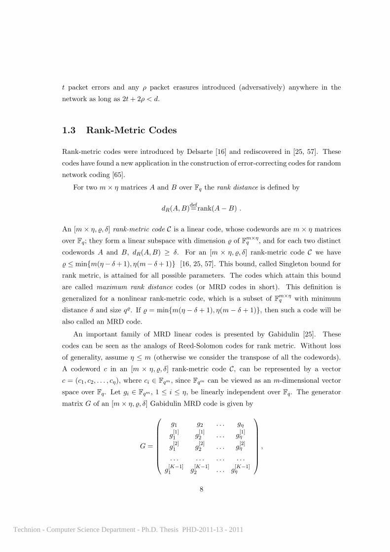
t packet errors and any ρ packet erasures introduced (adversatively) anywhere in the
network as long as 2t+ 2ρ < d.
1.3 Rank-Metric Codes
Rank-metric codes were introduced by Delsarte [16] and rediscovered in [25, 57]. These
codes have found a new application in the construction of error-correcting codes for random
network coding [65].
For two m× η matrices A and B over Fq the rank distance is defined by
dR(A,B)def=rank(A−B) .
An [m× η, ϱ, δ] rank-metric code C is a linear code, whose codewords are m× η matrices
over Fq; they form a linear subspace with dimension ϱ of Fm×ηq , and for each two distinct
codewords A and B, dR(A,B) ≥ δ. For an [m × η, ϱ, δ] rank-metric code C we have
ϱ ≤ min{m(η− δ+1), η(m− δ+1)} [16, 25, 57]. This bound, called Singleton bound for
rank metric, is attained for all possible parameters. The codes which attain this bound
are called maximum rank distance codes (or MRD codes in short). This definition is
generalized for a nonlinear rank-metric code, which is a subset of Fm×ηq with minimum
distance δ and size qϱ. If ϱ = min{m(η − δ + 1), η(m− δ + 1)}, then such a code will be
also called an MRD code.
An important family of MRD linear codes is presented by Gabidulin [25]. These
codes can be seen as the analogs of Reed-Solomon codes for rank metric. Without loss
of generality, assume η ≤ m (otherwise we consider the transpose of all the codewords).
A codeword c in an [m × η, ϱ, δ] rank-metric code C, can be represented by a vector
c = (c1, c2, . . . , cη), where ci ∈ Fqm , since Fqm can be viewed as an m-dimensional vector
space over Fq. Let gi ∈ Fqm , 1 ≤ i ≤ η, be linearly independent over Fq. The generator
matrix G of an [m× η, ϱ, δ] Gabidulin MRD code is given by
G =
g1 g2 . . . gη
g[1]1 g
[1]2 . . . g
[1]η
g[2]1 g
[2]2 . . . g
[2]η
. . . . . . . . . . . .
g[K−1]1 g
[K−1]2 . . . g
[K−1]η
,
8
Technion - Computer Science Department - Ph.D. Thesis PHD-2011-13 - 2011

where K = η − δ + 1, ϱ = mK, and [i] = qi mod m.
1.4 Related Work
1.4.1 Bounds
Let Aq(n, d) denotes the maximum number of codewords in an (n,M, d) code in projective
space, and let Aq(n, 2δ, k) denotes the maximum number of codewords in an (n,M, 2δ, k)
constant dimension code. (Note that the distance between any two elements in Gq(n, k) isalways even).
Without loss of generality we will assume that k ≤ n − k. This assumption can be
justified as a consequence of the following lemma [22].
Lemma 1 If C is an (n,M, d, k)q constant dimension code then C⊥ = {X⊥ : X ∈ C},where X⊥ is the orthogonal subspace of X, is an (n,M, d, n−k)q constant dimension code.
Let Sn,k(X, t) denotes a sphere of radius t in Gq(n, k) centered at a subspaceX ∈ Gq(n, k).It was proved [43] that the volume of Sn,k(X, t) is independent on X, since the Grass-
mann graph, corresponding to Gq(n, k), is distance regular. Then we denote the volume
of a sphere of radius t in Gq(n, k) by |Sn,k(t)|.
Lemma 2 [43] Let t ≤ k. Then
|Sn,k(t)| =t∑
i=0
qi2
[k
i
]q
[n− k
i
]q
.
Koetter and Kschischang [43] established the following sphere-packing and sphere-
covering bounds for Aq(n, 2δ, k):
Theorem 1 (Sphere-packing bound) Let t =⌊δ−12
⌋. Then
Aq(n, 2δ, k) ≤|Gq(n, k)||Sn,k(t)|
=
[n
k
]q
t∑i=0
qi2[
k
i
]q
[n− k
i
]q
. (1.2)
9
Technion - Computer Science Department - Ph.D. Thesis PHD-2011-13 - 2011

Theorem 2 (Sphere-covering bound)
Aq(n, 2δ, k) ≥|Gq(n, k)|
|Sn,k(δ − 1)|=
[n
k
]q
δ−1∑i=0
qi2[
k
i
]q
[n− k
i
]q
. (1.3)
Koetter and Kschischang [43] also developed the Singleton-type bound, which is always
stronger than the sphere-packing bound (1.2):
Theorem 3 (Singleton bound)
Aq(n, 2δ, k) ≤
[n− δ + 1
k − δ + 1
]q
. (1.4)
Xia in [77] showed a Graham-Sloane type lower bound:
Theorem 4
Aq(n, 2δ, k) ≥
(q − 1)
[n
k
]q
(qn − 1)qn(δ−2).
However, this bound is weaker than the bound (1.3).
Wang, Xing and Safavi-Naini [76] introduced the linear authentication codes. They
showed that an (n,M, 2δ, k)q constant dimension code is exactly an [n,M, n− k, δ] lin-
ear authentication code over GF (q). They also established an upper bound on linear
authentication codes, which is equivalent to the following bound on constant dimension
codes:
Theorem 5
Aq(n, 2δ, k) ≤
[n
k − δ + 1
]q[
k
k − δ + 1
]q
. (1.5)
This bound was proved by using a different method by Etzion and Vardy in [21, 22].
This method based on bounds on anticodes in the Grassmannian. In [78] was shown that
10
Technion - Computer Science Department - Ph.D. Thesis PHD-2011-13 - 2011

the bound (1.5) is always stronger than the Singleton bound (1.4). Furthermore, it was
proved [21, 22] that the codes known as Steiner structures attain the bound (1.5).
The following Johnson-type bounds were presented in [21, 22, 78]:
Theorem 6 (Johnson bounds)
Aq(n, 2δ, k) ≤qn − 1
qk − 1Aq(n− 1, 2δ, k − 1), (1.6)
Aq(n, 2δ, k) ≤qn − 1
qn−k − 1Aq(n− 1, 2δ, k). (1.7)
Using bounds (1.6), and (1.7) recursively, and combining with the observation that
Aq(n, 2δ, k) = 1 for all k < 2δ, the following bound is obtained [21, 22, 78]:
Theorem 7
Aq(n, 2δ, k) ≤⌊qn − 1
qk − 1
⌊qn−1 − 1
qk−1 − 1· · ·⌊qn−k+δ − 1
qδ − 1
⌋· · ·⌋⌋
.
The upper and lower bounds on Aq(n, 2δ, k) when δ = k were considered in [21, 22]:
Theorem 8
Aq(n, 2k, k) ≤⌊qn − 1
qk − 1
⌋− 1, if k - n, (1.8)
Aq(n, 2k, k) =qn − 1
qk − 1, if k | n, (1.9)
Aq(n, 2k, k) ≥qn − qk(qr − 1)− 1
qk − 1, where n ≡ r (mod k). (1.10)
The following two bounds on Aq(n, d) are presented in [21, 22].
Theorem 9 (Gilbert-Varshamov bound)
Aq(n, d) ≥|Pq(n)|2
n∑k=0
d−1∑j=0
j∑i=0
[n− k
j − i
]q
[k
i
]q
[n
k
]q
qi(j−i)
.
This lower bound generalize the Gilbert-Varshamov bound for graphs that are not
necessarily distance-regular.
The following upper bound on Aq(n, d) [21, 22] is obtained by using a linear program-
ming (LP) method.
11
Technion - Computer Science Department - Ph.D. Thesis PHD-2011-13 - 2011

Theorem 10 (LP bound)
Aq(n, 2e+ 1) ≤ f⋆,
where f⋆ = max {D0 +D1 + · · ·Dn}, subject to the following 2n+ 2 linear constraints:
e∑j=−e
c(i+ j, i, e)Di+j ≤
[n
i
]q
and Di ≤ Aq(n, 2e+ 2, i),
for all 0 ≤ i ≤ n, where Di denote the number of codewords with dimension i and c(k, i, e)
denote the size of the set {X : ds(X,Y ) ≤ e, dimX = i} for a k-dimensional subspace Y .
1.4.2 Constructions of Codes
Koetter and Kschischang [43] presented a construction of Reed-Solomon like constant
dimension codes. They showed that these codes attain the Singleton bound asymptotically.
Silva, Koetter, and Kschischang [65] showed that this construction can be described
in terms of rank-metric codes.
Let A be an m×η matrix over Fq, and let Im be an m×m identity matrix. The matrix
[Im A] can be viewed as a generator matrix of an m-dimensional subspace of Fm+ηq . This
subspace is called the lifting of A [65].
Example 1 Let A and [I3 A] be the following matrices over F2
A =
1 1 0
0 1 1
0 0 1
, [I3 A] =
1 0 0 1 1 0
0 1 0 0 1 1
0 0 1 0 0 1
,
then the 3-dimensional subspace X, the lifting of A, is given by the following 8 vectors:
X = ({100110), (010011), (001001), (110101),
(101111), (011010), (111100), (000000)}.
A constant dimension code C ⊆ Gq(n, k) such that all its codewords are lifted codewords
of a rank-metric code C ⊆ Fk×(n−k)q , i.e., C = {row space[Ik A] : A ∈ C}, is called the
lifting of C [65].
12
Technion - Computer Science Department - Ph.D. Thesis PHD-2011-13 - 2011

Theorem 11 [65] If C is a [k×(n−k), ϱ, δ] rank-metric code, then the constant dimension
code C obtained by the lifting of C is an (n, qϱ, 2δ, k)q code.
A constant dimension code C such that all its codewords are lifted codewords of an
MRD code is called a lifted MRD code [65]. This code will be denoted by CMRD.
Manganiello, Gorla and Rosenthal [53] showed the construction of spread codes, i.e.
codes that have the maximal possible distance in the Grassmannian. This construction
can be viewed as a generalization of the lifted MRD code construction.
Skachek [67] provided a recursive construction for constant dimension codes, which can
be viewed as a generalization of the construction in [53].
Gadouleau and Yan [27] proposed a construction of constant dimension codes based
on constant rank codes.
Etzion and Vardy [21, 22] introduced a construction of codes in Gq(n, k) based on a
Steiner structure, that attain the bound (1.5). They proved that any Steiner structure
Sq(t, k, n) is an (n,M, 2δ, k) code in Gq(n, k) with M =
[n
t
]q
/
[k
t
]q
and δ = k − t+ 1.
They also developed computational methods to search for the codes with a certain struc-
ture, such as cyclic codes, in Pq(n).
Kohnert and Kurz [44] described a construction of constant dimension codes in terms
of 0− 1 integer programming. However, the dimensions of such an optimization problem
are very large in this context. It was shown in [44] that by prescribing a group of au-
tomorphisms of a code, it is possible significantly reduce the size of the problem. Large
codes with constant dimension k = 3 and n ≤ 14 were constructed by using this method.
Remark 1 Silva and Kschischang [66] proposed a new subspace metric, called the injec-
tion metric, for error correction in network coding, given by
dI(X,Y ) = max{dim(X),dim(Y )} − dim(X ∩ Y ),
for any two subspaces X,Y ∈ Pq(n). It was shown [66] that codes in Pq(n) designed for dI
may have higher rates than those designed for dS. The injection distance and the subspace
distance are closely related [66]:
dI(X,Y ) =1
2dS(X,Y ) +
1
2|dim(X)− dim(Y )|,
13
Technion - Computer Science Department - Ph.D. Thesis PHD-2011-13 - 2011

therefore, these two metrics are equivalent for the Grassmannian. The bounds and con-
structions of codes in Pq(n) for the injection metric are presented in [26], [39], and [40].
1.5 Organization of This Work
The rest of this thesis is organized as follows. In Chapter 2 we discuss different representa-
tions of subspaces in the projective space and present a new formula for the computation
of the distance between any two different subspaces in Pq(n). In Section 2.1 we consider
the representations of subspaces in Pq(n). We define the reduced row echelon form of a
k-dimensional subspace and its Ferrers diagram. These two concepts combined with the
identifying vector of a subspace will be our main tools for the representation of subspaces.
In Section 2.2 we present a formula for an efficient computation of the distance between
two subspaces in the projective space.
In Chapter 3 we consider lifted MRD codes. In Section 3.1 we discuss properties of
these codes related to block designs. We prove that the codewords of a lifted MRD code
form a design called a transversal design, a structure which is known to be equivalent
to the well known orthogonal array. We also prove that the same codewords form a
subspace transversal design, which is akin to the transversal design, but not its q-analog.
In Section 3.2 we show that these designs can be used to derive a new family of linear
codes in the Hamming space, and in particular, LDPC codes. We provide upper and lower
bounds on the minimum distance, the stopping distance and the dimension of such codes.
We prove that there are no small trapping sets in such codes. We prove that some of these
codes are quasi-cyclic and attain the Griesmer bound.
In Chapter 4 we present new bounds and constrictions for constant dimension codes.
In Section 4.1 we present the multilevel construction. This construction requires rank-
metric codes in which some of the entries are forced to be zeroes due to constraints given
by the Ferrers diagram. We first present an upper bound on the size of such codes. We
show how to construct some rank-metric codes which attain this bound. Next, we describe
the multilevel construction of the constant dimension codes. First, we select a constant
weight code C. Each codeword of C defines a skeleton of a basis for a subspace in reduced
row echelon form. This skeleton contains a Ferrers diagram on which we design a rank-
metric code. Each such rank-metric code is lifted to a constant dimension code. The
union of these codes is our final constant dimension code. We discuss the parameters of
these codes and also their decoding algorithms. In Section 4.2 we derive upper bounds
14
Technion - Computer Science Department - Ph.D. Thesis PHD-2011-13 - 2011

on codes that contain lifted MRD codes, based on their combinatorial structure, and
provide constructions for two families of codes that attain these upper bounds. The first
construction can be considered as a generalization of the multilevel method presented in
Section 4.1. This construction based also on an one-factorization of a complete graph. The
second construction is based on the existence of a 2-parallelism in Gq(4, 2). In Section 4.3
we generalize the well-known concept of a punctured code for a code in the projective
space. Puncturing in the projective space is more complicated than its counterpart in the
Hamming space. The punctured codes of our constant dimension codes have larger size
than the codes obtained by using the multilevel approach described in Section 4.1. We
discuss the parameters of the punctured code and also its decoding algorithm.
The main goal of Chapter 5 is to present efficient enumerative encoding and decoding
techniques for the Grassmannian and to describe a general search method for constant
dimension lexicodes. In Section 5.1 we present two lexicographic orders for the Grassman-
nian, based on different representations of subspaces in the Grassmannian. In Section 5.2
we describe the enumerative coding methods, based on different lexicographic orders, and
discuss their computation complexity. Section 5.3 deals with constant dimension lexicodes.
Finally, we conclude with Chapter 6, where we summarize our results and present a
list of open problems for further research.
15
Technion - Computer Science Department - Ph.D. Thesis PHD-2011-13 - 2011

Chapter 2
Representations of Subspaces and
Distance Computation
In this chapter we first consider different representations of a subspace in Pq(n). The
constructions for codes in Pq(n) and Gq(n, k), the enumerative coding methods, and the
search for lexicodes, presented in the following chapters, are based on these representations.
Next, we present a new formula for the computation of the distance of two different
subspaces in Pq(n). This formula enables to simplify the computations that lead to the
next subspace in the search for a constant dimension lexicode which will be described in
the sequel.
2.1 Representations of Subspaces
In this section we define the reduced row echelon form of a k-dimensional subspace and its
Ferrers diagram. These two concepts combined with the identifying vector of a subspace
will be our main tools for the representation of subspaces. We also define and discuss
some types of integer partitions which have an important role in our exposition.
2.1.1 Reduced Row Echelon Form Representation
A matrix is said to be in row echelon form if each nonzero row has more leading zeroes
than the previous row.
The results presented in this chapter were published in [62] and [63].
16
Technion - Computer Science Department - Ph.D. Thesis PHD-2011-13 - 2011

A k × n matrix with rank k is in reduced row echelon form (RREF) if the following
conditions are satisfied.
• The leading coefficient (pivot) of a row is always to the right of the leading coefficient
of the previous row.
• All leading coefficients are ones.
• Each leading coefficient is the only nonzero entry in its column.
A k-dimensional subspace X of Fnq can be represented by a k × n generator matrix
whose rows form a basis for X. There is exactly one such matrix in RREF and it will be
denoted by RE(X). For simplicity, we will assume that the entries in RE(X) are taken
from Zq instead of Fq, using an appropriate bijection.
Example 2 We consider the 3-dimensional subspace X of F72 with the following eight
elements.
1) (0 0 0 0 0 0 0)
2) (1 0 1 1 0 0 0)
3) (1 0 0 1 1 0 1)
4) (1 0 1 0 0 1 1)
5) (0 0 1 0 1 0 1)
6) (0 0 0 1 0 1 1)
7) (0 0 1 1 1 1 0)
8) (1 0 0 0 1 1 0)
.
The subspace X can be represented by a 3×7 generator matrix whose rows form a basis for
the subspace. There are 168 different matrices for the 28 different bases. Many of these
matrices are in row echelon form. One of them is1 0 1 0 0 1 1
0 0 1 1 1 1 0
0 0 0 1 0 1 1
.
17
Technion - Computer Science Department - Ph.D. Thesis PHD-2011-13 - 2011

Exactly one of these 168 matrices is in reduced row echelon form:
RE(X) =
1 0 0 0 1 1 0
0 0 1 0 1 0 1
0 0 0 1 0 1 1
.
2.1.2 Ferrers Tableaux Form Representation
Partitions
A partition of a positive integer t is a representation of t as a sum of positive integers, not
necessarily distinct. We order this collection of integers in a decreasing order.
A Ferrers diagram F represents a partition as a pattern of dots with the i-th row
having the same number of dots as the i-th term in the partition [5, 51, 68]. In the sequel,
a dot will be denoted by a ” • ”. A Ferrers diagram satisfies the following conditions.
• The number of dots in a row is at most the number of dots in the previous row.
• All the dots are shifted to the right of the diagram.
Remark 2 Our definition of Ferrers diagram is slightly different from the usual defini-
tion [5, 51, 68], where the dots in each row are shifted to the left of the diagram.
Let |F| denotes the size of a Ferrers diagram F , i.e., the number of dots in F . The
number of rows (columns) of the Ferrers diagram F is the number of dots in the rightmost
column (top row) of F . If the number of rows in the Ferrers diagram is m and the number
of columns is η we say that it is an m× η Ferrers diagram.
If we read the Ferrers diagram by columns we get another partition which is called
the conjugate of the first one. If the partition forms an m × η Ferrers diagram then the
conjugate partition forms an η ×m Ferrers diagram.
Example 3 Assume we have the partition 6 + 5 + 5 + 3 + 2 of 21. The 5 × 6 Ferrers
18
Technion - Computer Science Department - Ph.D. Thesis PHD-2011-13 - 2011
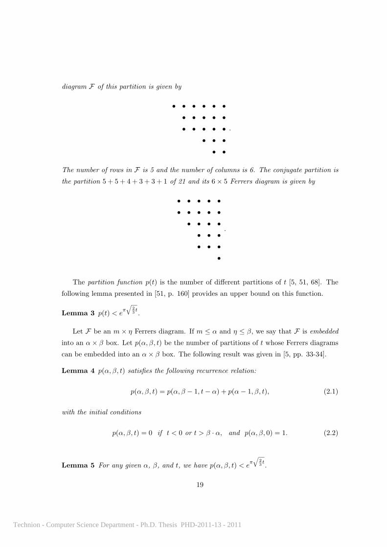
diagram F of this partition is given by
• • • • • •• • • • •• • • • •
• • •• •
.
The number of rows in F is 5 and the number of columns is 6. The conjugate partition is
the partition 5 + 5 + 4 + 3 + 3 + 1 of 21 and its 6× 5 Ferrers diagram is given by
• • • • •• • • • •
• • • •• • •• • •
•
.
The partition function p(t) is the number of different partitions of t [5, 51, 68]. The
following lemma presented in [51, p. 160] provides an upper bound on this function.
Lemma 3 p(t) < eπ√
23t.
Let F be an m× η Ferrers diagram. If m ≤ α and η ≤ β, we say that F is embedded
into an α× β box. Let p(α, β, t) be the number of partitions of t whose Ferrers diagrams
can be embedded into an α× β box. The following result was given in [5, pp. 33-34].
Lemma 4 p(α, β, t) satisfies the following recurrence relation:
p(α, β, t) = p(α, β − 1, t− α) + p(α− 1, β, t), (2.1)
with the initial conditions
p(α, β, t) = 0 if t < 0 or t > β · α, and p(α, β, 0) = 1. (2.2)
Lemma 5 For any given α, β, and t, we have p(α, β, t) < eπ√
23t.
19
Technion - Computer Science Department - Ph.D. Thesis PHD-2011-13 - 2011

Proof: Clearly, p(α, β, t) ≤ p(t), where p(t) is the number of unrestricted partitions of t.
Then by Lemma 3 we have that p(t) < eπ√
23tand thus p(α, β, t) < e
π√
23t.
The following theorem [51, p. 327] provides a connection between the q-ary Gaussian
coefficients and partitions.
Theorem 12 For any given integers k and n, 0 < k ≤ n,
[n
k
]q
=
k(n−k)∑t=0
αtqt,
where αt = p(k, n− k, t).
Ferrers Tableaux Form Representation
For each X ∈ Gq(n, k) we associate a binary vector of length n and weight k, denoted
by v(X), called the identifying vector of X, where the ones in v(X) are exactly in the
positions where RE(X) has the leading ones.
Example 4 Consider the 3-dimensional subspace X of Example 2. Its identifying vector
is v(X) = 1011000.
Remark 3 We can consider an identifying vector v(X) for some k-dimensional subspace
X as a characteristic vector of a k-subset. This coincides with the definition of rank-
and order-preserving map ϕ from Gq(n, k) onto the lattice of subsets of an n-set, given by
Knuth [41] and discussed by Milne [54].
The echelon Ferrers form of a binary vector v of length n and weight k, denoted by
EF(v), is the k×n matrix in RREF with leading entries (of rows) in the columns indexed
by the nonzero entries of v and “•” in all entries which do not have terminal zeroes or ones.
This notation is also given in [51, 68]. The dots of this matrix form the Ferrers diagram Fof EF(v). Let v(X) be the identifying vector of a subspace X ∈ Gq(n, k). Its echelon
Ferrers form EF(v(X)) and the corresponding Ferrers diagram, denoted by FX , will be
called the echelon Ferrers form and the Ferrers diagram of the subspace X, respectively.
20
Technion - Computer Science Department - Ph.D. Thesis PHD-2011-13 - 2011

Example 5 For the vector v = 1011000, the echelon Ferrers form EF(v) is the following
3× 7 matrix:
EF(v) =
1 • 0 0 • • •0 0 1 0 • • •0 0 0 1 • • •
.
The Ferrers diagram of EF(v) is given by
• • • •• • •• • •
.
Remark 4 All the binary vectors of the length n and weight k can be considered as the
identifying vectors of all the subspaces in Gq(n, k). These(nk
)vectors partition Gq(n, k) into
the(nk
)different classes, where each class consists of all the subspaces in Gq(n, k) with the
same identifying vector. These classes are called Schubert cells [24, p. 147]. Note that
each Schubert cell contains all the subspaces with the same given echelon Ferrers form.
The Ferrers tableaux form of a subspace X, denoted by F(X), is obtained by assigning
the values of RE(X) in the Ferrers diagram FX of X. In other words, F(X) is obtained
from RE(X) first by removing from each row of RE(X) the zeroes to the left of the leading
coefficient; and after that removing the columns which contain the leading coefficients. All
the remaining entries are shifted to the right. Each Ferrers tableaux form represents a
unique subspace in Gq(n, k).
Example 6 Let X be a subspace in G2(7, 3) from Example 2. Its echelon Ferrers form,
Ferrers diagram, and Ferrers tableaux form are given by1 • 0 0 • • •0 0 1 0 • • •0 0 0 1 • • •
,
• • • •• • •• • •
, and
0 1 1 0
1 0 1
0 1 1
, respectively .
2.1.3 Extended Representation
Let X ∈ Gq(n, k) be a k-dimensional subspace. The extended representation, EXT(X),
of X is a (k + 1) × n matrix obtained by combining the identifying vector v(X) =
21
Technion - Computer Science Department - Ph.D. Thesis PHD-2011-13 - 2011

(v(X)n, . . . , v(X)1) and the RREF RE(X) = (Xn, . . . , X1), as follows
EXT(X) =
(v(X)n . . . v(X)2 v(X)1
Xn . . . X2 X1
).
Note, that v(X)n is the most significant bit of v(X). Also, Xi is a column vector and
v(X)i is the most significant bit of the column vector
(v(X)i
Xi
).
Example 7 Consider the 3-dimensional subspace X of Example 2. Its extended repre-
sentation is given by
EXT(X) =
1 0 1 1 0 0 0
1 0 0 0 1 1 0
0 0 1 0 1 0 1
0 0 0 1 0 1 1
.
The extended representation is redundant since the RREF defines a unique subspace.
Nevertheless, we will see in the sequel that this representation will lead to more efficient
enumerative coding. Some insight for this will be the following well known equality given
in [51, p. 329].
Lemma 6 For all integers q, k, and n, such that k ≤ n we have[n
k
]q
= qk
[n− 1
k
]q
+
[n− 1
k − 1
]q
. (2.3)
The lexicographic order of the Grassmannian that will be discussed in Section 5.1 is based
on Lemma 6 (applied recursively). Note that the number of subspaces in which v(X)1 = 1
is
[n− 1
k − 1
]q
and the number of subspaces in which v(X)1 = 0 is qk[
n− 1
k
]q
.
2.2 Distance Computation
The research on error-correcting codes in the projective space in general and on the search
for lexicodes in the Grassmannian (which will be considered in the sequel) in particular,
requires many computations of the distance between two subspaces in Pq(n). The moti-
22
Technion - Computer Science Department - Ph.D. Thesis PHD-2011-13 - 2011

vation is to simplify the computations that lead to the next subspace which will be joined
to a lexicode.
Let A ∗ B denotes the concatenation
(A
B
)of two matrices A and B with the same
number of columns. By the definition of the subspace distance (1.1), it follows that
dS(X,Y ) = 2 rank(RE(X) ∗ RE(Y ))− rank(RE(X))− rank(RE(Y )). (2.4)
Therefore, the computation of dS(X,Y ) can be done by using Gauss elimination. In
this section we present an improvement on this computation by using the representation of
subspaces by Ferrers tableaux forms, from which their identifying vectors and their RREF
are easily determined. We will present an alternative formula for the computation of the
distance between two subspaces X and Y in Pq(n).
For X ∈ Gq(n, k1) and Y ∈ Gq(n, k2), let ρ(X,Y ) [µ(X,Y )] be a set of coordinates with
common zeroes [ones] in v(X) and v(Y ), i.e.,
ρ(X,Y ) = {i| v(X)i = 0 and v(Y )i = 0}
and
µ(X,Y ) = {i| v(X)i = 1 and v(Y )i = 1} .
Note that |ρ(X,Y )| + |µ(X,Y )| + dH(v(X), v(Y )) = n, where dH(·, ·) denotes the
Hamming distance, and
|µ(X,Y )| = k1 + k2 − dH(v(X), v(Y ))
2. (2.5)
Let Xµ be the |µ(X,Y )| × n sub-matrix of RE(X) which consists of the rows with
leading ones in the columns related to (indexed by) µ(X,Y ). Let XµC be the (k1 −|µ(X,Y )|) × n sub-matrix of RE(X) which consists of all the rows of RE(X) which are
not contained in Xµ. Similarly, let Yµ be the |µ(X,Y )| × n sub-matrix of RE(Y ) which
consists of the rows with leading ones in the columns related to µ(X,Y ). Let YµC be the
(k2 − |µ(X,Y )|)× n sub-matrix of RE(Y ) which consists of all the rows of RE(Y ) which
are not contained in Yµ.
Let Xµ be the |µ(X,Y )| × n sub-matrix of RE(RE(X) ∗ YµC ) which consists of the
rows with leading ones in the columns indexed by µ(X,Y ). Intuitively, Xµ obtained
by concatenation of the two matrices, RE(X) and YµC , and ”cleaning” (by adding the
23
Technion - Computer Science Department - Ph.D. Thesis PHD-2011-13 - 2011

corresponding rows of YµC ) all the nonzero entries in columns of RE(X) indexed by leading
ones in YµC . Finally, Xµ is obtained by taking only the rows which are indexed by µ(X,Y ).
Thus, Xµ has all-zero columns indexed by ones of v(Y ) and v(X) which are not in µ(X,Y ).
Hence Xµ has nonzero elements only in columns indexed by ρ(X,Y ) ∪ µ(X,Y ).
Let Yµ be the |µ(X,Y )|×n sub-matrix of RE(RE(Y )∗XµC ) which consists of the rows
with leading ones in the columns indexed by µ(X,Y ). Similarly to Xµ, it can be verified
that Yµ has nonzero elements only in columns indexed by ρ(X,Y ) ∪ µ(X,Y ).
Corollary 1 Nonzero entries in Xµ− Yµ can appear only in columns indexed by ρ(X,Y ).
Proof: An immediate consequence from the definition of Xµ and Yµ, since the columns
of Xµ and Yµ indexed by µ(X,Y ) form a |µ(X,Y )| × |µ(X,Y )| identity matrix.
Theorem 13
dS(X,Y ) = dH(v(X), v(Y )) + 2dR(Xµ, Yµ). (2.6)
Proof: By (2.4) it is sufficient to proof that
2 rank(RE(X) ∗ RE(Y )) = k1 + k2 + dH(v(X), v(Y )) + 2dR(Xµ, Yµ). (2.7)
It is easy to verify that
rank
(RE(X)
RE(Y )
)= rank
RE(X)
YµC
Yµ
= rank
RE(X)
YµC
Yµ
= rank
(RE(RE(X) ∗ YµC )
Yµ
)= rank
(RE(RE(X) ∗ YµC )
Yµ − Xµ
). (2.8)
We note that the positions of the leading ones in all the rows of RE(X) ∗ YµC are in
{1, 2, . . . , n} \ ρ(X,Y ). By Corollary 1, the positions of the leading ones of all the rows of
RE(Yµ − Xµ) are in ρ(X,Y ). Thus, by (2.8) we have
rank(RE(X) ∗ RE(Y )) = rank(RE(RE(X) ∗ YµC ) + rank(Yµ − Xµ). (2.9)
Since the sets of positions of the leading ones of RE(X) and YµC are disjoint, we have
24
Technion - Computer Science Department - Ph.D. Thesis PHD-2011-13 - 2011

that rank(RE(X) ∗ YµC ) = k1 + (k2 − |µ(X,Y )|), and thus, by (2.9) we have
rank(RE(X) ∗ RE(Y )) =k1 + k2 − |µ(X,Y )|+ rank(Yµ − Xµ). (2.10)
Combining (2.10) and (2.5) we obtain
2 rank(RE(X) ∗ RE(Y )) = k1 + k2 + dH(v(X), v(Y )) + 2dR(Yµ, Xµ),
and by (2.7) this proves the theorem.
The following two results will play an important role in our constructions for error-
correcting codes in the projective space and in our search for constant dimension lexicodes.
Corollary 2 For any two subspaces X,Y ∈ Pq(n),
dS(X,Y ) ≥ dH(v(X), v(Y )).
Corollary 3 Let X and Y be two subspaces in Pq(n) such that v(X) = v(Y ). Then
dS(X,Y ) = 2 rank(RE(X)− RE(Y )).
25
Technion - Computer Science Department - Ph.D. Thesis PHD-2011-13 - 2011
Chapter 3
Codes and Designs Related to
Lifted MRD Codes
There is a close connection between error-correcting codes in the Hamming space and
combinatorial designs. For example, the codewords of weight 3 in the Hamming code
form a Steiner triple system, MDS codes are equivalent to orthogonal arrays, Steiner
systems (if exist) form optimal constant weight codes [1].
The well-known concept of q-analogs replaces subsets by subspaces of a vector space
over a finite field and their orders by the dimensions of the subspaces. In particular, the
q-analog of a constant weight code in the Hamming space is a constant dimension code in
the projective space. Related to constant dimension codes are q-analogs of block designs.
q-analogs of designs were studied in [1, 9, 22, 23, 59, 71]. For example, in [1] it was shown
that Steiner structures (the q-analog of Steiner system), if exist, yield optimal codes in
the Grassmannian. Another connection is the constructions of constant dimension codes
from spreads which are given in [22] and [53].
In this chapter we consider the lifted MRD codes. We prove that the codewords of
such a code form a design called a transversal design, a structure which is known to be
equivalent to the well known orthogonal array. We also prove that the same codewords
form a subspace transversal design, which is akin to the transversal design, but not its
q-analog. The incidence matrix of the transversal design derived from a lifted MRD code
can be viewed as a parity-check matrix of a linear code in the Hamming space. This way
to construct linear codes from designs is well-known [3, 36, 38, 45, 48, 49, 74, 75]. We find
The material in this chapter was presented in part in [64].
26
Technion - Computer Science Department - Ph.D. Thesis PHD-2011-13 - 2011

the properties of these codes which can be viewed also as LDPC codes.
3.1 Lifted MRD Codes and Transversal Designs
MRD codes can be viewed as maximum distance separable (MDS) codes [25], and as such
they form combinatorial designs known as orthogonal arrays and transversal designs [29].
We consider some properties of lifted MRD codes which are derived from their combina-
torial structure. These properties imply that lifted MRD codes yield transversal designs
and orthogonal arrays with other parameters. Moreover, the codewords of these codes
form the blocks of a new type of transversal designs, called subspace transversal designs.
3.1.1 Properties of Lifted MRD Codes
Recall, that a lifted MRD code CMRD (defined in Subsection 1.4.2) is a constant dimension
code such that all its codewords are the lifted codewords of an MRD code.
For simplicity, in the sequel we will consider only the linear MRD codes constructed
by Gabidulin [25], which are presented in Section 1.3. It does not restrict our discussion as
such codes exist for all parameters. However, even lifted nonlinear MRD codes also have
all the properties and results which we consider (with a possible exception of Lemma 10).
Theorem 14 [65] If C is a [k × (n − k), (n − k)(k − δ + 1), δ] MRD code, then its lifted
code CMRD is an (n, q(n−k)(k−δ+1), 2δ, k)q code.
The parameters of the [k × (n− k), (n− k)(k − δ + 1), δ] MRD code C in Theorem 14
implies by the definition of an MRD code that k ≤ n− k. Hence, all our results are only
for k ≤ n−k. The results cannot be generalized for k > n−k (for example Lemma 9 does
not hold for k > n−k unless δ = 1 which is a trivial case). We will also assume that k > 1.
Let L be the set of qn − qn−k vectors of length n over Fq in which not all the first k
entries are zeroes. The following lemma is a simple observation.
Lemma 7 All the nonzero vectors which are contained in codewords of CMRD belong to L.
For a set S ⊆ Fnq , let ⟨S⟩ denotes the subspace of Fn
q spanned by the elements of S. If
S = {v} is of size one, then we denote ⟨S⟩ by ⟨v⟩. Let V = {⟨v⟩ : v ∈ L} be the set ofqn−qn−k
q−1 one-dimensional subspaces of Fnq whose nonzero vectors are contained in L. We
identify each one-dimensional subspace A in Gq(ω, 1), for any given ω, with the vector
vA ∈ A (of length ω) in which the first nonzero entry is an one.
27
Technion - Computer Science Department - Ph.D. Thesis PHD-2011-13 - 2011

For each A ∈ Gq(k, 1) we define
VAdef={X | X = ⟨v⟩, v = vAz, z ∈ Fn−k
q }.
{VA : A ∈ Gq(k, 1)} contains qk−1q−1 sets, each one of the size qn−k. These sets partition the
set V, i.e., these sets are disjoint and V =∪
A∈Gq(k,1)VA. We say that a vector v ∈ Fn
q is in
VA if v ∈ X for X ∈ VA. Clearly, ⟨{vAz′, vAz′′}⟩, for A ∈ Gq(k, 1) and z′ = z′′, contains
a vector with k leading zeroes, which does not belong to L. Hence, by Lemma 7 we have
Lemma 8 For each A ∈ Gq(k, 1), a codeword of CMRD contains at most one element
from VA.
Note that each k-dimensional subspace of Fnq contains
[k
1
]q
= qk−1q−1 one-dimensional
subspaces. Therefore, by Lemma 7, each codeword of CMRD contains qk−1q−1 elements of V.
Hence, by Lemma 8 and since |Gq(k, 1)| = qk−1q−1 we have
Corollary 4 For each A ∈ Gq(k, 1), a codeword of CMRD contains exactly one element
from VA.
Lemma 9 Each (k − δ + 1)-dimensional subspace Y of Fnq , whose nonzero vectors are
contained in L, is contained in exactly one codeword of CMRD.
Proof: Let Sdef={Y ∈ Gq(n, k − δ + 1) : |Y ∩ L| = qk−δ+1 − 1}, i.e. S consists of all
(k − δ + 1)-dimensional subspaces of Gq(n, k − δ + 1) in which all the nonzero vectors are
contained in L.Since the minimum distance of CMRD is 2δ and its codewords are k-dimensional sub-
spaces, it follows that the intersection of any two codewords is at most of dimension k− δ.
Hence, each (k− δ+1)-dimensional subspace of Fnq is contained in at most one codeword.
The size of CMRD is q(n−k)(k−δ+1), and the number of (k − δ + 1)-dimensional subspaces
in a codeword is exactly
[k
k − δ + 1
]q
. By Lemma 7, each (k − δ + 1)-dimensional sub-
space, of a codeword, is contained in S. Hence, the codewords of CMRD contain exactly[k
k − δ + 1
]q
q(n−k)(k−δ+1) distinct (k − δ + 1)-dimensional subspaces of S.
To complete the proof we only have to show that S does not contain more (k− δ+1)-
dimensional subspaces. Hence, we will compute the size of S. Each element of S intersects
with each VA, A ∈ Gq(k, 1) in at most one 1-dimensional subspace. There are
[k
k − δ + 1
]q
28
Technion - Computer Science Department - Ph.D. Thesis PHD-2011-13 - 2011

ways to choose an arbitrary (k−δ+1)-dimensional subspace of Fkq . For each such subspace
Y we choose an arbitrary basis {x1, x2, . . . , xk−δ+1} and denote Ai = ⟨xi⟩, 1 ≤ i ≤ k−δ+1.
A basis for a (k − δ + 1)-dimensional subspace of S will be generated by concatenation of
xi with a vector z ∈ Fn−kq for each i, 1 ≤ i ≤ k − δ + 1. Therefore, there are q(k−δ+1)(n−k)
ways to choose a basis for an element of S. Hence, |S| =[
k
k − δ + 1
]q
q(n−k)(k−δ+1).
Thus, the lemma follows.
Corollary 5 Each (k − δ − i)-dimensional subspace of Fnq , whose nonzero vectors are
contained in L, is contained in exactly q(n−k)(i+1) codewords of CMRD.
Proof: The size of CMRD is q(n−k)(k−δ+1). The number of (k−δ−i)-dimensional subspaces
in a codeword is exactly
[k
k − δ − i
]q
. Hence, the total number of (k− δ− i)-dimensional
subspaces in CMRD is
[k
k − δ − i
]q
q(n−k)(k−δ+1). Similarly to the proof of Lemma 9, we
can prove that the total number of (k−δ−i)-dimensional subspaces which contain nonzero
vectors only from L is
[k
k − δ − i
]q
q(n−k)(k−δ−i). Thus, each (k − δ − i)-dimensional
subspace of Fnq , whose nonzero vectors are contained in L, is contained in exactly
[k
k − δ − i
]q
q(n−k)(k−δ+1)
[k
k − δ − i
]q
q(n−k)(k−δ−i)
= q(n−k)(i+1)
codewords of CMRD.
Corollary 6 Any one-dimensional subspace X ∈ V is contained in exactly q(n−k)(k−δ)
codewords of CMRD.
Corollary 7 Any two elements X1, X2 ∈ V, such that X1 ∈ VA and X2 ∈ VB, A = B,
are contained in exactly q(n−k)(k−δ−1) codewords of CMRD.
Proof: Apply Corollary 5 with k − δ − i = 2.
Lemma 10 CMRD can be partitioned into q(n−k)(k−δ) sets, called parallel classes, each
one of size qn−k, such that in each parallel class each element of V is contained in exactly
one codeword.
29
Technion - Computer Science Department - Ph.D. Thesis PHD-2011-13 - 2011
Proof: First we prove that a lifted MRD code contains a lifted MRD subcode with
disjoint codewords (subspaces). Let G be the generator matrix of a [k × (n − k), (n −k)(k − δ + 1), δ] MRD code C [25], n− k ≥ k. Then G has the following form
G =
g1 g2 . . . gk
gq1 gq2 . . . gqk...
... · · ·...
gqk−δ
1 gqk−δ
2 . . . gqk−δ
k
,
where gi ∈ Fqn−k are linearly independent over Fq. If the last k− δ rows are removed from
G, the result is an MRD subcode of C with the minimum distance k. In other words, an
[k × (n− k), n− k, k] MRD subcode C of C is obtained. The corresponding lifted code is
an (n, qn−k, 2k, k)q lifted MRD subcode of CMRD.
Let C1 = C, C2, . . . , Cq(n−k)(k−δ) be the q(n−k)(k−δ) cosets of C in C. All these q(n−k)(k−δ)
cosets are nonlinear rank-metric codes with the same parameters as the [k×(n−k), n−k, k]
MRD code. Therefore, their lifted codes form a partition of CMRD into q(n−k)(k−δ) parallel
classes each one of size qn−k, such that each element of V is contained in exactly one
codeword of each parallel class.
3.1.2 Transversal Designs from Lifted MRD Codes
A transversal design of groupsize m, blocksize k, strength t and index λ, denoted by
TDλ(t, k,m) is a triple (V,G,B), where
1. V is a set of km elements (called points);
2. G is a partition of V into k classes (called groups), each one of size m;
3. B is a collection of k-subsets of V (called blocks);
4. each block meets each group in exactly one point;
5. every t-subset of points that meets each group in at most one point is contained in
exactly λ blocks.
When t = 2, the strength is usually not mentioned, and the design is denoted by TDλ(k,m).
A TDλ(t, k,m) is resolvable if the set B can be partitioned into sets B1, ...,Bs, where each
element of V is contained in exactly one block of each Bi. The sets B1, ...,Bs are called
parallel classes.
30
Technion - Computer Science Department - Ph.D. Thesis PHD-2011-13 - 2011

Example 8 Let V = {1, 2, . . . , 12}; G = {G1, G2, G3}, where G1 = {1, 2, 3, 4}, G2 =
{5, 6, 7, 8}, and G = {9, 10, 11, 12}; B = {B1, B2, . . . , B16}, where B1 = {1, 5, 9}, B2 =
{2, 8, 11}, B3 = {3, 6, 12}, B4 = {4, 7, 10}, B5 = {1, 6, 10}, B6 = {2, 7, 12}, B7 =
{3, 5, 11}, B8 = {4, 8, 9}, B9 = {1, 7, 11}, B10 = {2, 6, 9}, B11 = {3, 8, 10}, B12 =
{4, 5, 12}, B13 = {1, 8, 12}, B14 = {2, 5, 10}, B15 = {3, 7, 9}, and B16 = {4, 6, 11}.These form a resolvable TD1(3, 4) with four parallel classes B1 = {B1, B2, B3, B4}, B2 =
{B5, B6, B7, B8}, B3 = {B9, B10, B11, B12}, and B4 = {B13, B14, B15, B16}.
Theorem 15 The codewords of an (n, q(n−k)(k−δ+1), 2δ, k)q code CMRD form the blocks
of a resolvable transversal design TDλ(qk−1q−1 , qn−k), λ = q(n−k)(k−δ−1), with q(n−k)(k−δ)
parallel classes, each one of size qn−k.
Proof: Let V be the set of qn−qn−k
q−1 points for the design. Each set VA, A ∈ Gq(k, 1),
is defined to be a group, i.e., there are qk−1q−1 groups, each one of size qn−k. The k-
dimensional subspaces (codewords) of CMRD are the blocks of the design. By Corollary 4,
each block meets each group in exactly one point. By Corollary 7, each 2-subset which
meets each group in at most one point is contained in exactly q(n−k)(k−δ−1) blocks. Finally,
by Lemma 10, the design is resolvable with q(n−k)(k−δ) parallel classes, each one of size
qn−k.
An N × k array A with entries from a set of s elements is an orthogonal array with
s levels, strength t and index λ, denoted by OAλ(N, k, s, t), if every N × t subarray of
A contains each t-tuple exactly λ times as a row. It is known [29] that a TDλ(k,m) is
equivalent to an orthogonal array OAλ(λ ·m2, k,m, 2).
Remark 5 By the equivalence of transversal designs and orthogonal arrays, we have that
an (n, q(n−k)(k−δ+1), 2δ, k)q code CMRD induces an OAλ(q(n−k)(k−δ+1), q
k−1q−1 , q
n−k, 2) with
λ = q(n−k)(k−δ−1).
Remark 6 A [k × (n − k), (n − k)(k − δ + 1), δ] MRD code C is an MDS code if it is
viewed as a code of length k over Fqn−k . Thus its codewords form an orthogonal array
OAλ(q(n−k)(k−δ+1), k, qn−k, k − δ + 1) with λ = 1 [29], which is also an orthogonal array
OAλ(q(n−k)(k−δ+1), k, qn−k, 2) with λ = q(n−k)(k−δ−1).
Now we define a new type of transversal designs in terms of subspaces, which will be
called a subspace transversal design. We will show that such a design is induced by the
31
Technion - Computer Science Department - Ph.D. Thesis PHD-2011-13 - 2011

codewords of a lifted MRD code. Moreover, in the following chapter we will show that
this design is useful to obtain upper bounds on the codes that contain the lifted MRD
codes, and in a construction of large constant dimension codes.
Let V0 be a set of one-dimensional subspaces in Gq(n, 1), that contains only vectors
starting with k zeroes. Note that V0 is isomorphic to Gq(n− k, 1).
A subspace transversal design of groupsize qm, m = n − k, block dimension k, and
strength t, denoted by STDq(t, k,m), is a triple (V,G,B), where
1. V is the subset of all elements of Gq(n, 1) \ V0, |V| = (qk−1)q−1 qm (the points);
2. G is a partition of V into qk−1q−1 classes of size qm (the groups);
3. B is a collection of k-dimensional subspaces which contain only points from V (the
blocks);
4. each block meets each group in exactly one point;
5. every t-dimensional subspace (with points from V) which meets each group in at
most one point is contained in exactly one block.
As a direct consequence form Lemma 9 and Theorem 15 we have the following theorem.
Theorem 16 The codewords of an (n, q(n−k)(k−δ+1), 2δ, k)q code CMRD form the blocks of
a resolvable STDq(k − δ + 1, k, n− k), with the set of points V and the set of groups VA,
A ∈ Gq(k, 1), defined previously in this section.
Remark 7 There is no known nontrivial q-analog of a block design with λ = 1 and t > 1.
An STDq(t, k,m) is very close to such a design.
Remark 8 An STDq(t, k, n− k) cannot exist if k > n− k, unless t = k. Recall, that the
case k > n− k was not considered in this section (see Theorem 14).
3.2 Linear Codes Derived from Lifted MRD Codes
In this section we study the properties of linear codes in the Hamming space whose parity-
check matrix is an incidence matrix of a transversal design derived from a lifted MRD code.
These codes may also be of interest as LDPC codes.
32
Technion - Computer Science Department - Ph.D. Thesis PHD-2011-13 - 2011

For each codewordX of a constant dimension code CMRD we define its binary incidence
vector x of length |V| = qn−qn−k
q−1 as follows: xz = 1 if and only if the point z ∈ V is
contained in X.
Let H be the |CMRD| × |V| binary matrix whose rows are the incidence vectors of
the codewords of CMRD. By Theorem 15, this matrix H is the incidence matrix of
TDλ(qk−1q−1 , q
n−k), with λ = q(n−k)(k−δ−1). Note that the rows of the incidence matrix H
correspond to the blocks of the transversal design, and the columns of H correspond to
the points of the transversal design. If λ = 1 in such a design (or, equivalently, δ = k − 1
for CMRD), then HT is an incidence matrix of a net, the dual structure to the transversal
design [51, p. 243].
An [N,K, d] linear code is a linear subspace of dimension K of FN2 with the minimum
Hamming distance d.
Let C be the linear code with the parity-check matrix H, and let CT be the linear
code with the parity-check matrix HT . This approach for construction of linear codes is
widely used for LDPC codes. For example, codes whose parity-check matrix is an incidence
matrix of a block design are considered in [3, 36, 38, 45, 48, 49, 75, 74]. Codes obtained
from nets and transversal designs are considered in [18], [37].
The parity-check matrix H corresponds to a bipartite graph, called the Tanner graph
of the code. The rows and the columns of H correspond to the two parts of the vertex set
of the graph, and the nonzero entries of H correspond the the edges of the graph.
Given TDλ(qk−1q−1 , qn−k), if λ = 1, then the corresponding Tanner graph has girth 6
(girth is the length of the shortest cycle). If λ ≥ 1, then the girth of the Tanner graph
is 4.
3.2.1 Parameters of Linear Codes Derived from CMRD
The code C has length qn−qn−k
q−1 and the code CT has length q(n−k)(k−δ+1). By Corollary 6,
each column of H has q(n−k)(k−δ) ones; since each k-dimensional subspace contains qk−1q−1
one-dimensional subspaces, each row has qk−1q−1 ones.
Remark 9 Note that if δ = k, then the column weight of H is one. Hence, the minimum
distance of C is 2. Moreover, CT consists only of the all-zero codeword. Thus, these codes
are not interesting and hence in the sequel we assume that δ ≤ k − 1.
Lemma 11 The matrix H obtained from an (n, q(n−k)(k−δ+1), 2δ, k)q CMRD code can be
decomposed into blocks, where each block is a qn−k × qn−k permutation matrix.
33
Technion - Computer Science Department - Ph.D. Thesis PHD-2011-13 - 2011

Proof: It follows from Lemma 10 that the related transversal design is resolvable.
In each parallel class each element of V is contained in exactly one codeword of CMRD.
Each class has qn−k codewords, each group has qn−k points, and each codeword meets
each group in exactly one point. This implies that each qn−k rows of H related to such a
class can be decomposed into qk−1q−1 qn−k × qn−k permutation matrices.
Example 9 The [12, 4, 6] code C and the [16, 8, 4] code CT are obtained from the (4, 16, 2, 2)2
lifted MRD code CMRD. The incidence matrix for corresponding transversal design TD1(3, 4)
(see Example 8) is given by the following 16× 12 matrix. The four rows above this matrix
represent the column vectors for the points of the design.
0 0 0 0 1 1 1 1 1 1 1 1
1 1 1 1 0 0 0 0 1 1 1 1
0 0 1 1 0 0 1 1 0 0 1 1
0 1 0 1 0 1 0 1 0 1 0 1
1 0 0 0 1 0 0 0 1 0 0 0
0 1 0 0 0 0 0 1 0 0 1 0
0 0 1 0 0 1 0 0 0 0 0 1
0 0 0 1 0 0 1 0 0 1 0 0
1 0 0 0 0 1 0 0 0 1 0 0
0 1 0 0 0 0 1 0 0 0 0 1
0 0 1 0 1 0 0 0 0 0 1 0
0 0 0 1 0 0 0 1 1 0 0 0
1 0 0 0 0 0 1 0 0 0 1 0
0 1 0 0 0 1 0 0 1 0 0 0
0 0 1 0 0 0 0 1 0 1 0 0
0 0 0 1 1 0 0 0 0 0 0 1
1 0 0 0 0 0 0 1 0 0 0 1
0 1 0 0 1 0 0 0 0 1 0 0
0 0 1 0 0 0 1 0 1 0 0 0
0 0 0 1 0 1 0 0 0 0 1 0
Corollary 8 All the codewords of the code C, associated with the parity-check matrix H,
and of the code CT , associated with the parity-check matrix HT , have even weights.
Proof: Let c be a codeword of C (CT ). Then Hc = 0 (HT c = 0), where 0 denotes the
all-zero column vector. Assume that c has an odd weight. Then there is an odd number of
columns of H (HT ) that can be added to obtain the all-zero column vector, and that is a
34
Technion - Computer Science Department - Ph.D. Thesis PHD-2011-13 - 2011

contradiction, since by Lemma 11, H (HT ) is an array consisting of permutation matrices.
Corollary 9 The minimum Hamming distance d of C and the minimum Hamming dis-
tance dT of CT are upper bounded by 2qn−k.
Proof: We take all the columns of H (HT ) corresponding to any two blocks of permu-
tation matrices mentioned in Lemma 11. These columns sums to all-zero column vector,
and hence we found 2qn−k depended columns in H (HT ). Thus d ≤ 2qn−k ( dT ≤ 2qn−k).
To obtain a lower bound on the minimum Hamming distance of these codes we need
the following theorem known as the Tanner bound [69].
Theorem 17 The minimum distance, dmin, of a linear code defined by an m× n parity-
check matrix H with constant row weight ρ and constant column weight γ satisfy
1. dmin ≥ n(2γ−µ2)γρ−µ2
;
2. dmin ≥ 2n(2γ+ρ−2−µ2)ρ(γρ−µ2)
,
where µ2 is the second largest eigenvalue of HTH.
To obtain a lower bound on d and dT we need to find the second largest eigenvalue of
HTH and HHT , respectively. Note that since the set of eigenvalues of HTH and HHT
is the same, it is sufficient to find only the eigenvalues of HTH.
The following lemma is derived from [13, p. 563].
Lemma 12 Let H be an incidence matrix for TDλ(k,m). The eigenvalues of HTH are
rk, r, and rk − kmλ with multiplicities 1, k(m− 1), and k − 1, respectively, where r is a
number of blocks that are incident with a given point.
By Corollary 6, r = q(n−k)(k−δ) in TDλ(qk−1q−1 , qn−k) with λ = q(n−k)(k−δ−1). Thus,
from Lemma 12 we obtain the spectrum of HTH.
Corollary 10 The eigenvalues of HTH are q(n−k)(k−δ) qk−1q−1 , q
(n−k)(k−δ), and 0 with mul-
tiplicities 1, qk−1q−1 (q
n−k − 1), and qk−1q−1 − 1, respectively.
35
Technion - Computer Science Department - Ph.D. Thesis PHD-2011-13 - 2011

Now, by Theorem 17 and Corollary 10, we have
Corollary 11
d ≥ qn−k(qk − 1)
qk − q,
dT ≥
{2k δ = k − 1, q = 2, k = n− k
4q(n−k)(δ−k+1) otherwise.
Proof: By Corollary 10, the second largest eigenvalues of HTH is µ2 = q(n−k)(k−δ).
We apply Theorem 17 and obtain lower bounds on d:
d ≥qn−k qk−1
q−1 (2q(n−k)(k−δ) − q(n−k)(k−δ))
q(n−k)(k−δ) qk−1q−1 − q(n−k)(k−δ)
=qn−k(qk − 1)
qk − q, (3.1)
d ≥2qn−k qk−1
q−1 (2q(n−k)(k−δ) + qk−1
q−1 − 2− q(n−k)(k−δ))
qk−1q−1 (q
(n−k)(k−δ) qk−1q−1 − q(n−k)(k−δ))
=qn−k(qk − 1)
qk − q2
q(n−k)(k−δ) + qk−1q−1 − 2)
q(n−k)(k−δ) qk−1q−1
. (3.2)
The expression in (3.1) is larger than the expression in (3.2). Thus, we have that
d ≥ qn−k(qk−1)qk−q
for all δ ≤ k − 1.
In a similar way, by using Theorem 17 we obtain lower bounds on dT :
dT ≥qn−k(2 qk−1
q−1 − q(n−k)(k−δ))
qk−1q−1 − 1
, (3.3)
dT ≥ 4q(n−k)(δ−k+1). (3.4)
Note that the expression in (3.3) is negative for δ < k−1. For δ = k−1 with k = n−k
and q = 2, the bound in (3.3) is larger than the bound in (3.4). Thus, we have dT ≥ 2k,
if δ = k − 1, q = 2, and k = n− k; and dT ≥ 4q(n−k)(δ−k+1), otherwise.
A stopping set S in a code C is a subset of the variable nodes, related to the columns
of H, in a Tanner graph of C such that all the neighbors of S are connected to S at least
twice. The size of the smallest stopping set is called the stopping distance of a code C.
The stopping distance depends on the specific Tanner graph, and therefore, on the specific
parity-check matrix H, and it is denoted by s(H). The stopping distance plays a role
36
Technion - Computer Science Department - Ph.D. Thesis PHD-2011-13 - 2011

in iterative decoding over the binary erasure channel similar to the role of the minimum
distance in maximum likelihood decoding [17]. It is easy to see that s(H) is less or equal
to the minimum distance of the code C.
It was shown in [81, Corollary 3] that the Tanner lower bound on the minimum distance
is also the lower bound on the stopping distance of a code with a parity-check matrix H,
then from Corollary 11 we have the following result.
Corollary 12 The stopping distance s(H) of C and the stopping distance s(HT ) of CT
satisfy
s(H) ≥ qn−k(qk − 1)
qk − q,
s(HT ) ≥
{2k δ = k − 1, q = 2, k = n− k
4q(n−k)(δ−k+1) otherwise.
We use the following result proved in [38, Theorem 1] to improve the lower bound on
s(HT ) and, therefore, on dT .
Lemma 13 Let H be an incidence matrix of blocks (rows) and points (columns) such that
each block contains exactly κ points, and each pair of distinct blocks intersects in at most
γ points. If Σ is a stopping set in the Tanner graph corresponding to HT , then
|Σ| ≥ κ
γ+ 1.
Corollary 13 s(HT ) ≥ qk−1qk−δ−1
+ 1.
Proof: By Lemma 13, with κ = qk−1q−1 and γ = qk−δ−1
q−1 , since any two codewords in a
lifted MRD code intersect in at most (k− δ)-dimensional subspace, we have the following
lower bound on the size of every stopping set of CT and, particulary, for the smallest
stopping set of CT
s(HT ) ≥ (qk − 1)/(q − 1)
(qk−δ − 1)/(q − 1)+ 1 =
qk − 1
qk−δ − 1+ 1.
Obviously, for all δ ≤ k− 1, this bound is larger or equal than the bound of Corollary 12,
and thus the result follows.
We summarize all the results about the minimum distances and the stopping distances
of C and CT obtained above in the following theorem.
37
Technion - Computer Science Department - Ph.D. Thesis PHD-2011-13 - 2011

Theorem 18
2qn−k ≥ d ≥ s(H) ≥ qn−k(qk − 1)
qk − q,
2qn−k ≥ dT ≥ s(HT ) ≥ qk − 1
qk−δ − 1+ 1.
Let dim(C) and dim(CT ) be the dimensions of C and CT , respectively. To obtain the
lower and upper bounds on dim(C) and dim(CT ) we need the following basic results from
linear algebra [32]. For a matrix A over a field F, let rankF(A) denotes the rank of A
over F.
Lemma 14 Let A be a ρ× η matrix, and let R be the field of real numbers. Then
• rankR(A) = rankR(AT ) = rankR(A
TA).
• If ρ = η and A is a symmetric matrix with the eigenvalue 0 of multiplicity t, then
rankR(A) = η − t.
Theorem 19
dim(C) ≥ qk − 1
q − 1− 1,
dim(CT ) ≥ q(n−k)(k−δ+1) − qk − 1
q − 1(qn−k − 1)− 1.
Proof: First, we observe that dim(C) = qk−1q−1 q
n−k − rankF2(H), and dim(CT ) =
q(n−k)(k−δ+1)−rankF2(HT ). Now, we obtain an upper bound on rankF2(H) = rankF2(H
T ).
Clearly, rankF2(H) ≤ rankR(H). By Corollary 10, the multiplicity of an eigenvalue 0 of
HTH is qk−1q−1 − 1. Hence by Lemma 14, rankF2(H) ≤ rankR(H) = rankR(H
TH) =qk−1q−1 q
n−k − ( qk−1q−1 − 1). Thus, dim(C) ≥ qk−1
q−1 qn−k − ( q
k−1q−1 q
n−k − ( qk−1q−1 − 1)) = qk−1
q−1 − 1,
and dim(CT ) ≥ q(n−k)(k−δ+1) − qk−1q−1 q
n−k + qk−1q−1 − 1.
Now, we obtain an upper bound on the dimension of the codes C and CT for odd q.
Theorem 20 Let q be a power of an odd prime number.
• If qk−1q−1 is odd, then
dim(C) ≤ qk − 1
q − 1− 1 and dim(CT ) ≤ q(n−k)(k−δ+1) − qk − 1
q − 1(qn−k − 1)− 1.
38
Technion - Computer Science Department - Ph.D. Thesis PHD-2011-13 - 2011

• If qk−1q−1 is even, then
dim(C) ≤ qk − 1
q − 1, and dim(CT ) ≤ q(n−k)(k−δ+1) − qk − 1
q − 1(qn−k − 1).
Proof: We compute the lower bound on rankF2(H) to obtain the upper bound on the
dimension of the codes C and CT . First, we observe that rankF2(H) ≥ rankF2(HTH).
By [10], the rank over F2 of an integral diagonalizable square matrix A is lower bounded
by the sum of the multiplicities of the eigenvalues of A that do not vanish modulo 2. We
consider now rankF2(HTH). By Corollary 10, the second eigenvalue of HTH is always
odd for odd q. If qk−1q−1 is odd, then the first eigenvalue of HTH is also odd. Hence, we sum
the multiplicities of the first two eigenvalues to obtain rankF2(HTH) ≥ 1+ qk−1
q−1 (qn−k−1).
If qk−1q−1 is even, then the first eigenvalue is even, and hence we take only the multiplicity of
the second eigenvalue to obtain rankF2(HTH) ≥ qk−1
q−1 (qn−k − 1). The result follows now
from the fact that the dimension of a code is equal to the difference between its length
and rankF2(H).
Remark 10 For even values of q the method used in the proof for Theorem 20 leads to a
trivial result, since in this case all the eigenvalues of HTH are even and thus by [10] we
have rankF2(HTH) ≥ 0. But clearly, by Lemma 11 we have rankF2(H) ≥ qn−k. Thus, for
even q, dim(C) ≤ qk−1q−1 q
n−k−qn−k = qn−k( qk−1q−1 −1), and dim(CT ) = q(n−k)(k−δ+1)−qn−k.
Note that for odd q and odd qk−1q−1 the lower and the upper bounds on the dimension
of C and CT are the same. Therefore, we have the following corollary.
Corollary 14 For odd q and odd qk−1q−1 the dimensions dim(C) and dim(CT ) of the codes
C and CT , respectively, satisfy dim(C) = qk−1q−1 − 1, and dim(CT ) = q(n−k)(k−δ+1) −
qk−1q−1 q
n−k + qk−1q−1 − 1 .
Remark 11 Some of the results presented in this subsection generalize the results given
in [37]. In particular, the lower bounds on the minimum distance and the bounds on the
dimension of LDPC codes (with girth 6) derived from lifted MRD codes coincide with the
bounds on LDPC codes from partial geometries considered in [37].
3.2.2 LDPC Codes Derived from CMRD
Low-density parity check (LDPC) codes, introduced by Gallager in 1960’s [28], are known
as Shannon limit approaching codes [60]. Kou, Lin, and Fossorier [45] presented the first
39
Technion - Computer Science Department - Ph.D. Thesis PHD-2011-13 - 2011

systematic construction of LDPC codes based on finite geometries. Their work started
a new research direction of algebraic constructions of LDPC codes. Many LDPC codes
were obtained from different combinatorial designs, such that balanced incomplete block
designs, Steiner triple systems, orthogonal arrays, and Latin squares [3, 36, 37, 38, 45,
48, 49, 74, 75].
LDPC codes are characterized by a sparse parity-check matrix with constant weight of
rows and constant weight of columns; and Tanner graph without cycles of length 4. Next,
we discuss LDPC codes derived from CMRD. Hence, in this subsection we consider only
TD1(qk−1q−1 , q
n−k), obtained from an (n, q2(n−k), 2(k − 1), k)q lifted MRD code.
Remark 12 It was pointed out in [70] that the codes based on finite geometries can per-
form well under iterative decoding despite many cycles of length 4 in their Tanner graphs.
Hence, also the codes mentioned in the previous subsection can be of interest from this
point of view.
Some parameters of LDPC codes obtained from lifted MRD codes compared with the
LDPC codes based on finite geometries [45] (FG in short) can be found in Table 3.1.
Table 3.1: LDPC codes from CMRD vs. LDPC codes from finite geometries
LDPC codes from FG LDPC codes from CMRD
[N,K, d] K/N [N,K, d] K/N
[273, 191, 18] 0.699 [240, 160, 18] 0.667
[4095, 3367, 65] 0.822 [4096, 3499,≥ 64] 0.854
[4161, 3431, 66] 0.825 [4032, 3304,≥ 66] 0.819
A code is called quasi-cyclic if there is an integer p such that every cyclic shift of a
codeword by p entries is again a codeword.
Let N(K, d) denotes the length of the shortest binary linear code of dimension K and
minimum distance d. Then by Griesmer bound [52] ,
N(K, d) ≥K−1∑i=0
⌈d
2i
⌉. (3.5)
Theorem 21 An LDPC code C obtained from an (n, 22(n−2), 2, 2)2 lifted MRD code CMRD
is a [2n − 2n−2, n, 2n−2n−2
2 ] quasi-cyclic code with p = 2n−2, which attains the Griesmer
bound.
40
Technion - Computer Science Department - Ph.D. Thesis PHD-2011-13 - 2011

Proof: First we prove that C is quasi-cyclic. Let T be the TD1(3, 2n−2) obtained from
an (n, 22(n−2), 2, 2)2 code CMRD. T has 3 groups Vi = {⟨v⟩|v = aiz, z ∈ Fn−2q }, 1 ≤ i ≤ 3,
where a1 = ⟨01⟩, a2 = ⟨10⟩, and a3 = ⟨11⟩. The first 2n−2 columns of the incidence matrix
H of T correspond to the points of V1, the next 2n−2 columns correspond to the points of
V2, and the last 2n−2 columns correspond to the points of V3. The suffices z ∈ Fn−22 for
the points of T are ordered lexicographically.
Let X = {0, v, u, w = v+ u} be a codeword of CMRD, where 0 is the all-zero vector of
length n, and v, u, w ∈ Fn2 . By Corollary 4, each codeword contains exactly one point from
each group, hence w.l.o.g. we write v = 01v′, u = 10u′, and w = 11w′, for v′, u′, w′ ∈ Fn−22 .
Let X ′ be a set of points corresponding to the cyclic shift of the incidence vector for X, by
2n−2 entries to the left. Then X ′ = {01u′, 10w′, 11v′}. Obviously, v′ + u′ = w′, and since
a code CMRD contains all the 2-dimensional subspaces with vectors from V, we have that
X ′∪{0} is also a codeword of CMRD. Therefore, if c is a codeword in C, and c′ is obtained
by the cyclic shift of c by 2n−k entries to the left, then Hc = 0 implies that Hc′ = 0.
Now we prove that C is a [2n − 2n−2, n, 2n−2n−2
2 ] code. Let K be the dimension of C.
First assume that K > n. By Theorem 18, d ≥ 3·2n−2
2 . Hence, by Griesmer bound (3.5)
we have:
2n − 2n−2 = 3 · 2n−2 ≥K−1∑i=0
⌈d
2i
⌉≥
K−1∑i=0
⌈3 · 2n−3
2i
⌉
≥n∑
i=3
3 · 2n−i +
⌈3
2
⌉+
⌈3
4
⌉+ (K − n) = 3 · 2n−2 − 3 + 3 + (K − n), (3.6)
contradiction, thus K ≤ n. Now assume that K < n. We form an n× (3 · 2n−2) matrix G,
such that its columns are the vectors for the points of T , where the first 2n−2 columns
correspond to the vectors of V1, next 2n−2 columns correspond to the vectors of V2, and
the last 2n−2 columns correspond to the vectors of V3, in the lexicographic order. By
the construction of H, and since the sum of all the vectors in a subspace equals to the
all-zero vector, we have that GHT = 0, therefore, the rows of G are the codewords of C.
Moreover, all the rows of G are linearly independent: for example, if we take the rows
in the following order: r2, rn, rn−1, rn−2, ..., r3, r1, where ri denotes the ith row of G, we
obtain a matrix in row echelon form. Therefore, K ≥ n, and thus we proved that K = n.
Hence, we have the equality in (3.6), and therefore, d = 3·2n−2
2 . Thus, the code C attains
the Griesmer bound.
41
Technion - Computer Science Department - Ph.D. Thesis PHD-2011-13 - 2011

Remark 13 The codes of Theorem 21 are equivalent to the punctured Hadamard codes [52].
It has been observed that for most LDPC codes that decoded with iterative message-
passing algorithms there exists a phenomenon, called error-floor [56]. This is a region,
where the error probability does not approaches zero as quickly at high SNRs as it does
at low SNRs. It is known that the error-floor of LDPC codes for AWGN channel is mostly
caused by the combinatorial structure, called trapping set [56]. A (κ, τ) trapping set of
a code C with a parity-check matrix H is defined as a set T (κ, τ) of size κ of the set of
columns of H, with κ ≥ 1 and τ ≥ 0, such that in the restriction of H to these κ columns,
there are exactly τ rows of odd weight.
It was shown that the trapping sets with small values κ and small ratios τ/κ contribute
significantly to high error-floors [56]. A (κ, τ) trapping set of an LDPC codes of length N
is called small if κ ≤√N and τ/κ ≤ 4 [47].
Let Cγ,ρ be a (γ, ρ)-regular LDPC code, i.e., a code with the constant column weight
γ and the constant row weight ρ of the parity-check matrix. Assume that its length is N
and the girth is at least six. In [33, 34] were proved two following theorems which show
that there are no (small) trapping sets in Cγ,ρ.
Theorem 22 There is no trapping set (κ, τ) in Cγ,ρ such that κ < γ + 1 and τ < γ.
Theorem 23 If 3 < γ ≤√N , then there is no small trapping set of size smaller than
γ − 3.
Now we apply these results on our LDPC codes derived form lifted MRD codes. Clearly,
these codes have girth six and they are regular codes with constant column weight γ = qn−k
for C and constant column weight γT = qk−1q−1 for CT ; moreover, qk−1
q−1 ≤√
q2(n−k). Hence,
we obtain the following results.
Corollary 15 There is no trapping set (κ, τ) in C such that κ < qn−k + 1 and τ < qn−k,
and there is no trapping set (κT , τT ) in CT such that κT < qk−1q−1 + 1 and τT < qk−1
q−1 .
Corollary 16 For all parameters q, k, n except for q = k = 2, there is no small trapping
set in CT of size smaller than qk−1q−1 − 3.
42
Technion - Computer Science Department - Ph.D. Thesis PHD-2011-13 - 2011

Chapter 4
New Bounds and Constructions
for Codes in Projective Space
4.1 Multilevel Construction via Ferrers Diagrams
Rank-Metric Codes
Our goal in this section is to generalize the construction of lifted MRD codes [65] in the
sense that these codes will be sub-codes of our codes and all our codes can be partitioned
into sub-codes, each one of them is a lifted rank-metric code (where some of the entries of
its codewords are forced to be zeroes). We use a multilevel approach to design our codes.
First, we select a constant weight code. Each codeword defines a skeleton of a basis for a
subspace in reduced row echelon form. This skeleton contains a Ferrers diagram on which
we design a rank-metric code. Each such rank-metric code is lifted to a constant dimension
code. The union of these codes is our final constant dimension code. The rank-metric codes
used for this construction form a new class of rank-metric codes, called Ferrers diagram
rank-metric codes. The multilevel construction will be applied to obtain error-correcting
constant dimension codes, but it can be adapted to construct error-correcting projective
space codes without any modification. We will also consider the parameters and decoding
algorithms for our codes. The efficiency of the decoding depends on the efficiency of the
decoding for the constant weight codes and the rank-metric codes.
The material of Section 4.1 and Section 4.3 is based on [20] and also was presented in [19]. Thematerial of Section 4.2 was presented in part in [64].
43
Technion - Computer Science Department - Ph.D. Thesis PHD-2011-13 - 2011

4.1.1 Ferrers Diagram Rank-Metric Codes
In this subsection we present rank-metric codes which will be used for our multilevel
construction for codes in the projective space. Our construction requires rank-metric
codes in which some of the entries are forced to be zeroes due to constraints given by the
Ferrers diagram. We present an upper bound on the size of such codes. We show how to
construct some rank-metric codes which attain this bound.
Let v be a vector of length n and weight k and let EF(v) be its echelon Ferrers form.
Let F be the Ferrers diagram of EF(v). F is anm×η Ferrers diagram, m ≤ k, η ≤ n−k. A
code C is an [F , ϱ, δ] Ferrers diagram rank-metric code if all codewords are m× η matrices
in which all entries not in F are zeroes, it forms a rank-metric code with dimension ϱ, and
minimum rank distance δ. Let dim(F , δ) be the largest possible dimension of an [F , ϱ, δ]
code.
Theorem 24 For a given i, 0 ≤ i ≤ δ − 1, if νi is the number of dots in F , which are
not contained in the first i rows and are not contained in the rightmost δ− 1− i columns,
then mini{νi} is an upper bound of dim(F , δ).
Proof: For a given i, 0 ≤ i ≤ δ − 1, let Ai be the set of the νi positions of F which are
not contained in the first i rows and are not contained in the rightmost δ− 1− i columns.
Assume the contrary that there exists an [F , νi+1, δ] code C. Let B = {B1, B2, . . . , Bνi+1}be a set of νi + 1 linearly independent codewords in C. Since the number of linearly
independent codewords is greater than the number of entries in Ai, there exists a nontrivial
linear combination Y =∑νi+1
j=1 αjBj for which the νi entries of Ai are equal zeroes. Y is
not the all-zero codeword since the Bi’s are linearly independent. F has outside Ai exactly
i rows and δ− i− 1 columns. These i rows can contribute at most i to the rank of Y and
the δ − i− 1 columns can contribute at most δ − i− 1 to the rank of Y . Therefore Y is a
nonzero codeword with rank less than δ, a contradiction.
Hence, an upper bound on dim(F , δ) is νi for each 0 ≤ i ≤ δ − 1. Thus, an upper
bound on the dimension dim(F , δ) is mini{νi}.
Conjecture 1 The upper bound of Theorem 24 is attainable for any given set of param-
eters q, F , and δ.
A code which attains the bound of Theorem 24 will be called a Ferrers diagram MRD
code. This definition generalizes the definition of MRD codes.
44
Technion - Computer Science Department - Ph.D. Thesis PHD-2011-13 - 2011

If we use i = 0 or i = δ − 1 in Theorem 24 then we obtain the following result.
Corollary 17 An upper bound on dim(F , δ) is the minimum number of dots that can be
removed from F such that the diagram remains with at most δ− 1 rows of dots or at most
δ − 1 columns of dots.
Remark 14 The [m × η, ϱ, δ] MRD codes are one class of Ferrers diagram rank-metric
codes which attain the bound of Corollary 17 with equality. In this case the Ferrers diagram
has m · η dots.
Example 10 Consider the following Ferrers diagram
F =
• • • •• •
••
and δ = 3. By Corollary 17 we have an upper bound, dim(F , 3) ≤ 2. But, if we use i = 1
in Theorem 24 then we have a better upper bound, dim(F , 3) ≤ 1. This upper bound is
attained with the following basis for an [F , 1, 3] rank-metric code.1 0 0 0
0 0 1 0
0 0 0 0
0 0 0 1
.
When the bound of Theorem 24 is attained? We start with a construction of Ferrers
diagram rank-metric codes which attain the bound of Corollary 17.
Assume we have an m × η, m = η + ε, ε ≥ 0, Ferrers diagram F , and that the
minimum in the bound of Corollary 17 is obtained by removing all the dots from the
η− δ+1 leftmost columns of F . Hence, only the dots in the δ− 1 rightmost columns will
remain. We further assume that each of the δ − 1 rightmost columns of F have m dots.
The construction which follows is based on the construction of MRD q-cyclic rank-metric
codes given by Gabidulin [25].
45
Technion - Computer Science Department - Ph.D. Thesis PHD-2011-13 - 2011

A code C of length m over Fqm is called a q-cyclic code if (c0, c1, ..., cm−1) ∈ C implies
that (cqm−1, cq0, ..., c
qm−2) ∈ C.
For a construction of [m×m, ϱ, δ] rank-metric codes, we use an isomorphism between
the field with qm elements, Fqm , and the set of all m-tuples over Fq, Fmq . We use the
obvious isomorphism by the representation of an element α in the extension field Fqm as
α = (α1, . . . , αm), where αi is an element in the ground field Fq.
Recall that a codeword c in an [m × m, ϱ, δ] rank-metric code C, can be represented
by a vector c = (c0, c1, . . . , cm−1), where ci ∈ Fqm and the generator matrix G of C is an
K × m matrix, ϱ = mK. It was proved by Gabidulin [25] that if C is an MRD q-cyclic
code then the generator polynomial of C is the linearized polynomial G(x) =m−K∑i=0
gixqi ,
where gi ∈ Fqm , gm−K = 1, m = K + δ − 1, and its generator matrix G has the following
form
g0 g1 · · · gm−K−1 1 0 · · · · · ·0 gq0 gq1 · · · gqm−K−1 1 · · · · · ·0 0 gq
2
0 · · · · · · gq2
m−K−1 1 · · ·· · · · · · · · · · · · · · · · · · · · · · · ·0 · · · · · · · · · · · · · · · gq
K−1
m−K−1 1
.
Hence, a codeword c ∈ C, c ∈ (Fqm)m, derived from the information word (a0, a1, . . . , aK−1),
where ai ∈ Fqm , i.e. c = (a0, a1, . . . , aK−1)G, has the form
c = (a0g0, a0g1 + a1gq0, . . . , aK−2 + aK−1g
qK−1
m−K−1, aK−1) .
We define an [m× η,m(η − δ + 1), δ] rank-metric code C′, m = η + ε, derived from Cas follows:
C′ = {(c0, c1, . . . , cη−1) : (0, . . . , 0, c0, c1, . . . , cη−1) ∈ C}.
Remark 15 C′ is also an MRD code.
We construct an [F , ℓ, δ] Ferrers diagram rank-metric code CF ⊆ C′, where F is an m× η
Ferrers diagram. Let γi, 1 ≤ i ≤ η, be the number of dots in column i of F , where the
columns are indexed from left to right. A codeword of CF is derived from a codeword of
46
Technion - Computer Science Department - Ph.D. Thesis PHD-2011-13 - 2011

c ∈ C by satisfying a set of m equations implied by
(a0g0, a0g1 + a1g
q0, . . . , aK−2 + aK−1g
qK−1
m−K−1, aK−1
)=
ε︷ ︸︸ ︷0...
0
. . .
0...
0
f1 . . . fK−ε
δ−1︷ ︸︸ ︷•...
•
. . .
•...
•
(4.1)
where fi = (• · · · •︸ ︷︷ ︸γi
0 · · · 0︸ ︷︷ ︸m−γi
)T is a column vector of length m, 1 ≤ i ≤ K− ε, and uT denotes
the transpose of the vector u. It is easy to verify that CF is a linear code.
By (4.1) we have a system ofm = K+δ−1 equations withK variables, a0, a1, . . . , aK−1.
The first ε equations implies that ai = 0 for 0 ≤ i ≤ ε − 1. The next K − ε = η − δ + 1
equations determine the values of the ai’s, ε ≤ i ≤ K − 1, as follows. From the next
equation aεgqε
0 = (• · · · •︸ ︷︷ ︸γ1
00...0︸ ︷︷ ︸m−γ1
)T (this is the next equation after we substitute ai = 0
for 0 ≤ i ≤ ε − 1), we have that aε has qγ1 solutions in Fqm , where each element of
Fqm is represented as an m-tuple over Fq. Given a solution of aε, the next equation
aεgqε
0 + aε+1gqε+1
1 = (• · · · •︸ ︷︷ ︸γ2
00...0︸ ︷︷ ︸m−γ2
)T has qγ2 solutions for aε+1. Therefore, we have that
a0, a1, . . . , aK−1 have q∑K−ε
i=1 γi solutions and hence the dimension of CF is∑K−ε
i=1 γi over
Fq. Note, that since each of the δ − 1 rightmost columns of F have m dots, i.e. γi = m,
K − ε + 1 ≤ i ≤ η (no zeroes in the related equations) it follows that any set of values
for the ai’s cannot cause any contradiction in the last δ − 1 equations. Also, since the
values of the K variables a0, a1, . . . , aK−1 are determined for the last δ − 1 equations, the
values for the related (δ− 1)m dots are determined. Hence, they do not contribute to the
number of solutions for the set of m equations. Thus, we have
Theorem 25 Let F be an m× η, m ≥ η, Ferrers diagram. Assume that each one of the
rightmost δ − 1 columns of F has m dots, and the i-th column from the left of F has γi
dots. Then CF is an [F ,∑η−δ+1
i=1 γi, δ] code which attains the bound of Corollary 17.
Remark 16 For any solution for variables a0, a1, . . . , aK−1 we have that (a0, a1, . . . , aK−1)G
= (0, . . . , 0, c0, c1, . . . , cη−1) ∈ C and (c0, c1, . . . , cη−1) ∈ CF .
Remark 17 For any [m × η,m(η − δ + 1), δ] rank-metric code C′, the codewords which
47
Technion - Computer Science Department - Ph.D. Thesis PHD-2011-13 - 2011

have zeroes in all the entries which are not contained in F form an [F ,∑η−δ+1
i=1 γi, δ] code.
Thus, we can use also any MRD codes, e.g., the codes described in [57], to obtain a proof
for Theorem 25.
Remark 18 Since CF is a subcode of an MRD code then we can use the decoding algorithm
of the MRD code for the decoding of our code. Also note, that if F is an m × η, m < η,
Ferrers diagram then we apply our construction for the η × m Ferrers diagram of the
conjugate partition.
When δ = 1 the bounds and the construction are trivial. If δ = 2 then by definition
the rightmost column and the top row of an m×η Ferrers diagram always has m dots and
η dots, respectively. It implies that the bound of Theorem 24 is always attained with the
construction if δ = 2. This is the most interesting case since in this case the improvement
of our constant dimension codes compared to the lifted MRD codes in [43, 65] is the most
impressive (see Subsection 4.1.4). If δ > 2 the improvement is relatively small, but we will
consider this case as it is of interest also from a theoretical point of view. We will give
two simple examples for constructions of Ferrers diagram MRD codes with δ = 3.
Example 11 Consider the following Ferrers diagram
F =
• • • •• • •
• ••
.
The upper bound on dim(F , 3) is 3. It is attained with the following basis with three 4× 4
matrices.
0 1 0 0
0 0 1 0
0 0 0 0
0 0 0 1
,
0 0 0 1
0 1 0 0
0 0 1 0
0 0 0 0
,
1 0 0 0
0 1 0 0
0 0 0 1
0 0 0 1
.
48
Technion - Computer Science Department - Ph.D. Thesis PHD-2011-13 - 2011

Example 12 Consider the following Ferrers diagram
F =
• • • •• • •• • •
•
.
The upper bound on dim(F , 3) is 4. It is attained with the basis consisting of four 4 × 4
matrices, from which three are from Example 11 and the last one is1 0 1 0
0 0 0 1
0 1 0 1
0 0 0 0
.
4.1.2 Lifted Ferrers Diagram Rank-Metric Codes
Usually a lifted MRD code CMRD is not maximal and it can be extended. This extension
requires to design rank-metric codes, where the shape of a codeword is a Ferrers diagram
rather than an k×(n−k) matrix. We would like to use the largest possible Ferrers diagram
rank-metric codes. In the appropriate cases, e.g., when δ = 2, for this purpose we will use
the Ferrers diagram MRD codes constructed in the previous subsection.
Assume we are given an echelon Ferrers form EF(v) of a binary vector v, of length n
and weight k, with a Ferrers diagram F and a Ferrers diagram rank-metric code CF . CFis lifted to a constant dimension code Cv by substituting each codeword A ∈ CF in the
columns of EF(v) which correspond to the zeroes of v, to obtain the generator matrix for
a codeword in Cv. Note, that depending on F it might implies conjugating F first. Unless
v starts with an one and ends with a zero (the cases in which F is a k × (n − k) Ferrers
diagram) we also need to expand the matrices of the Ferrers diagram rank-metric code to
k × (n − k) matrices (which will be lifted), where F is in their upper right corner (and
the new entries are zeroes). As an immediate consequence from Theorem 11 we have the
following.
Lemma 15 If CF is an [F , ϱ, δ] Ferrers diagram rank-metric code then its lifted code Cv,
related to an k × n echelon Ferrers form EF(v), is an (n, qϱ, 2δ, k)q constant dimension
code.
49
Technion - Computer Science Department - Ph.D. Thesis PHD-2011-13 - 2011

Example 13 For the word v = 1110000, its echelon Ferrers form
EF(v) =
1 0 0 • • • •0 1 0 • • • •0 0 1 • • • •
,
the 3× 4 matrix 1 0 1 0
0 0 0 1
0 0 0 0
is lifted to the 3-dimensional subspace with the 3× 7 generator matrix
1 0 0 1 0 1 0
0 1 0 0 0 0 1
0 0 1 0 0 0 0
.
For the word v = 1001001, its echelon Ferrers form
EF(v) =
1 • • 0 • • 0
0 0 0 1 • • 0
0 0 0 0 0 0 1
,
the 2× 4 matrix (1 0 1 0
0 0 0 1
)is lifted to the 3-dimensional subspace with the 3× 7 generator matrix
1 1 0 0 1 0 0
0 0 0 1 0 1 0
0 0 0 0 0 0 1
.
A lifted MRD code described in [65] can be considered as a lifted Ferrers diagram
MRD code, where its identifying vector is (1 . . . 10 . . . 0). If our lifted codes are the codes
constructed in Section 4.1.1 then the same decoding algorithm can be applied. Therefore,
the decoding in [65] for the corresponding constant dimension code can be applied directly
to each of our lifted Ferrers diagram MRD codes in this case, e.g. it can always be applied
50
Technion - Computer Science Department - Ph.D. Thesis PHD-2011-13 - 2011

when δ = 2. It would be worthwhile to permute the coordinates in a way that the identity
matrix Ik will appear in the first k columns, from the left, of the reduced row echelon
form, and F will appear in the upper right corner of the k× n matrix. The reason is that
the decoding of [65] is described on such matrices.
4.1.3 Multilevel Construction
Assume we want to construct an (n,M, 2δ, k)q constant dimension code C.
• The first step in the construction is to choose a binary constant weight code C of
length n, weight k, and minimum distance 2δ. This code will be called the skeleton
code. Any constant weight code can be chosen for this purpose, but different skeleton
codes will result in different constant dimension codes with usually different sizes.
The best choice for the skeleton code C will be discussed in the next subsection.
The next three steps are performed for each codeword c ∈ C.
• The second step is to construct the echelon Ferrers form EF(c).
• The third step is to construct an [F , ϱ, δ] Ferrers diagram rank-metric code CF for
the Ferrers diagram F of EF(c). If possible we will construct a code as described in
Subsection 4.1.1.
• The fourth step is to lift CF to a constant dimension code Cc, for which the echelon
Ferrers form of X ∈ Cc is EF(c).
Finally,
C =∪c∈C
Cc .
Recall that by Corollary 2, for any two subspaces X,Y ⊆ Fnq , we have that dS(X,Y ) ≥
dH(v(X), v(Y )). Hence, as an immediate consequence of Corollary 2 and Lemma 15 we
have the following theorem.
Theorem 26 C is an (n,M, 2δ, k)q constant dimension code, where M =∑
c∈C |Cc|.
51
Technion - Computer Science Department - Ph.D. Thesis PHD-2011-13 - 2011

Example 14 Let n = 6, k = 3, and C = {111000, 100110, 010101, 001011} be a constant
weight code of length 6, weight 3, and minimum Hamming distance 4. The echelon Ferrers
forms of these 4 codewords are
EF(111000) =
1 0 0 • • •0 1 0 • • •0 0 1 • • •
, EF(100110) =
1 • • 0 0 •0 0 0 1 0 •0 0 0 0 1 •
,
EF(010101) =
0 1 • 0 • 0
0 0 0 1 • 0
0 0 0 0 0 1
, EF(001011) =
0 0 1 • 0 0
0 0 0 0 1 0
0 0 0 0 0 1
.
By Theorem 25, the Ferrers diagrams of these four echelon Ferrers forms yield Ferrers
diagram MRD codes of sizes 64, 4, 2, and 1, respectively. Hence, we obtain a (6, 71, 4, 3)2
constant dimension code C.
Remark 19 A (6, 77, 4, 3)2 code was obtained by computer search [44]. Similarly, we
obtain a (7, 289, 4, 3)2 code. A (7, 304, 4, 3)2 code was obtained by computer search [44].
Example 15 Let C be the codewords of weight 4 in the [8, 4, 4] extended Hamming code
with the following parity-check matrix.0 0 0 0 1 1 1 1
0 0 1 1 0 0 1 1
0 1 0 1 0 1 0 1
1 1 1 1 1 1 1 1
C has 14 codewords with weight 4. Each one of these codewords is considered as an identi-
fying vector for the echelon Ferrers forms from which we construct the final (8, 4573, 4, 4)2
code C. The fourteen codewords of C and their contribution for the final code C are given
in Table 4.1. The codewords are taken in lexicographic order.
52
Technion - Computer Science Department - Ph.D. Thesis PHD-2011-13 - 2011
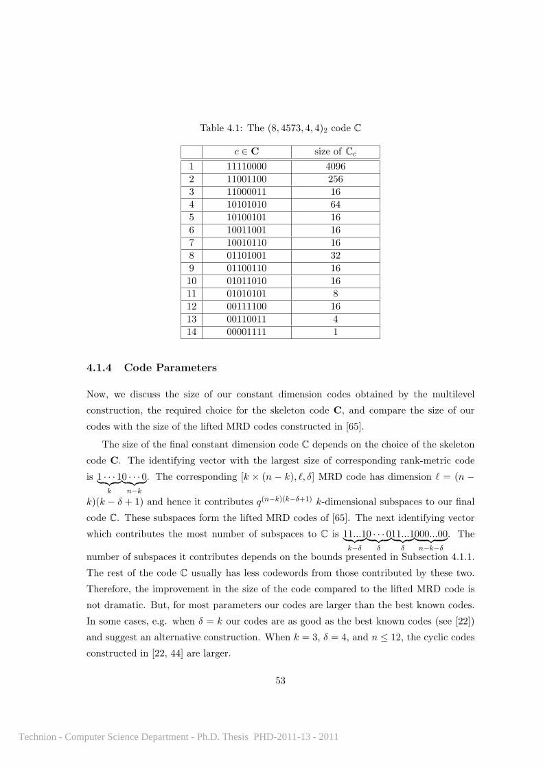
Table 4.1: The (8, 4573, 4, 4)2 code C
c ∈ C size of Cc
1 11110000 4096
2 11001100 256
3 11000011 16
4 10101010 64
5 10100101 16
6 10011001 16
7 10010110 16
8 01101001 32
9 01100110 16
10 01011010 16
11 01010101 8
12 00111100 16
13 00110011 4
14 00001111 1
4.1.4 Code Parameters
Now, we discuss the size of our constant dimension codes obtained by the multilevel
construction, the required choice for the skeleton code C, and compare the size of our
codes with the size of the lifted MRD codes constructed in [65].
The size of the final constant dimension code C depends on the choice of the skeleton
code C. The identifying vector with the largest size of corresponding rank-metric code
is 1 · · · 1︸ ︷︷ ︸k
0 · · · 0︸ ︷︷ ︸n−k
. The corresponding [k × (n − k), ℓ, δ] MRD code has dimension ℓ = (n −
k)(k − δ + 1) and hence it contributes q(n−k)(k−δ+1) k-dimensional subspaces to our final
code C. These subspaces form the lifted MRD codes of [65]. The next identifying vector
which contributes the most number of subspaces to C is 11...1︸ ︷︷ ︸k−δ
0 · · · 0︸ ︷︷ ︸δ
11...1︸ ︷︷ ︸δ
000...00︸ ︷︷ ︸n−k−δ
. The
number of subspaces it contributes depends on the bounds presented in Subsection 4.1.1.
The rest of the code C usually has less codewords from those contributed by these two.
Therefore, the improvement in the size of the code compared to the lifted MRD code is
not dramatic. But, for most parameters our codes are larger than the best known codes.
In some cases, e.g. when δ = k our codes are as good as the best known codes (see [22])
and suggest an alternative construction. When k = 3, δ = 4, and n ≤ 12, the cyclic codes
constructed in [22, 44] are larger.
53
Technion - Computer Science Department - Ph.D. Thesis PHD-2011-13 - 2011

Two possible alternatives for the best choice for the skeleton code C might be of special
interest. The first one is for k = 4 and n which is a power of two. We conjecture that
the best skeleton code is constructed from the codewords with weight 4 of the extended
Hamming code for which the columns of the parity-check matrix are given in lexicographic
order. We generalize this choice of codewords from the Hamming code by choosing a
constant weight lexicode [14]. Such a code is constructed as follows. All vectors of length
n and weight k are listed in lexicographic order. The code C is generated by adding to
the code C one codeword at a time. At each stage, the first codeword of the list that
does not violate the distance constraint with the other codewords of C, is joined to C.
Lexicodes are not necessarily the best constant weight codes. For example, the largest
constant weight code of length 10 and weight 4 is 30, while the lexicode with the same
parameters has size 18. But, the constant dimension code derived from the lexicode is
larger than any constant dimension code derived from any related code of size 30.
Table 4.2 summarized the sizes of some of our codes, denoted by CML, obtained by
the multilevel construction compared to the sizes of lifted MRD codes CMRD. In all these
codes we have started with a constant weight lexicode in the first step of the construction.
Table 4.2: CML vs. CMRD
q dS(C) n k |CMRD| |CML|2 4 9 4 215 215+4177
2 4 10 5 220 220+118751
2 4 12 4 224 224+2290845
2 6 10 5 215 215+73
2 6 13 4 218 218+4357
2 8 21 5 232 232+16844809
3 4 7 3 38 38+124
3 4 8 4 312 312+8137
4 4 7 3 48 48+345
4 4 8 4 412 412+72529
4.1.5 Decoding
The decoding of our codes is quite straightforward and it mainly consists of known decod-
ing algorithms. As we used a multilevel coding we will also need a multilevel decoding. In
the first step we will use a decoding for our skeleton code and in the second step we will
54
Technion - Computer Science Department - Ph.D. Thesis PHD-2011-13 - 2011

use a decoding for the rank-metric codes.
Assume the received word was a k-dimensional subspace Y . We start by generating its
reduced row echelon form RE(Y ). Given RE(Y ) it is straightforward to find the identifying
vector v(Y ). Now, we use the decoding algorithm for the constant weight code to find
the identifying vector v(X) of the submitted k-dimensional subspace X. If no more than
δ − 1 errors occurred then we will find the correct identifying vector. This claim is an
immediate consequence of Corollary 2.
In the second step of the decoding we are given the received subspace Y , its identifying
vector v(Y ), and the identifying vector v(X) of the submitted subspace X. We consider
the echelon Ferrers form EF(v(X)), its Ferrers diagram F , and the [F , ϱ, δ] Ferrers diagram
rank-metric code associated with it. We can permute the columns of EF(v(X)), and use
the same permutation on Y , in a way that the identity matrix Ik will be in the left side.
Now, we can use the decoding of the specific rank-metric code. If our rank-metric codes
are those constructed in Subsection 4.1.1 then we can use the decoding as described in [65].
It is clear now that the efficiency of our decoding depends on the efficiency of the decoding
of our skeleton code and the efficiency of the decoding of our rank-metric codes. If the
rank-metric codes are MRD codes then they can be decoded efficiently [25, 57]. The same
is true if the Ferrers diagram metric codes are those constructed in Subsection 4.1.1 as
they are subcodes of MRD codes and the decoding algorithm of the related MRD code
applied to them too.
There are some alternative ways for our decoding, some of which improve on the
complexity of the decoding. For example we can make use of the fact that most of the
code is derived from two identifying vectors or that most of the rank-metric codes are of
relatively small size. One such case can be when all the identity matrices of the echelon
Ferrers forms are in consecutive columns of the codeword (see [67]).
Finally, if we allow to receive a word which is an ℓ-dimensional subspace Y , k−δ+1 ≤ℓ ≤ k + δ − 1, then the same procedure will work as long as dS(X,Y ) ≤ δ − 1. This is a
consequence of the fact that the decoding algorithm of [65] does not restrict the dimension
of the received word.
55
Technion - Computer Science Department - Ph.D. Thesis PHD-2011-13 - 2011
4.2 Bounds and Constructions for Constant Dimension
Codes that Contain CMRD
Most of the constructions for constant dimension codes known in the literature produce
codes which contain CMRD [20, 27, 53, 63, 65, 67, 73]. The only constructions which
generate codes that do not contain CMRD are given in [22, 44]. These constructions are
either of so called orbit codes or specific constructions for small parameters. Moreover,
only (n,M, d, 3)2 orbit codes (specifically cyclic codes) with 8 ≤ n ≤ 12, and (6, 77, 4, 3)2
and (7, 304, 4, 3)2 codes are the largest codes for their specific parameters which do not
contain CMRD [44]. This motivates the question, what is the largest constant dimension
code which contain CMRD?
In this section we consider upper bounds and constructions for constant dimension
codes which contain the lifted MRD code. First, we consider two types of upper bounds
on the size of constant dimension codes, presented in [21, 22, 43, 76]. We estimate the
size of lifted MRD codes and codes generated by the multilevel construction relatively to
these bounds. Next, we discuss upper bounds on the size of constant dimension codes
which contain CMRD. In particular we prove that if an (n,M, 2(k− 1), k)q code C, k ≥ 3,
contains the (n, q2(n−k), 2(k − 1), k)q lifted MRD code then
M ≤ q2(n−k) +Aq(n− k, 2(k − 2), k − 1) .
We also present a construction for codes which either attain this bound or almost
attain it for k = 3. These codes are the largest known (n,M, 4, 3)q codes for n ≥ 13.
We prove that if an (n,M, 2k, 2k)q code C contains the (n, q(n−2k)(k+1), 2k, 2k)q lifted
MRD code then
M ≤ q(n−2k)(k+1) +
[n− 2k
k
]q
qn − qn−2k
q2k − qk+Aq(n− 2k, 2k, 2k) .
We present a construction for codes which attain this bound when k = 2, n = 8, and
for all q. These codes are the largest known for the related parameters.
56
Technion - Computer Science Department - Ph.D. Thesis PHD-2011-13 - 2011

4.2.1 Upper Bounds for Constant Dimension Codes
In this subsection we discuss two upper bounds for constant dimension codes presented in
Theorem 3 (the Singleton bound) and Theorem 5, given by
Aq(n, 2δ, k) ≤
[n− δ + 1
k − δ + 1
]q
(4.2)
and
Aq(n, 2δ, k) ≤
[n
k − δ + 1
]q[
k
k − δ + 1
]q
. (4.3)
It was proved in [43] that the ratio of the size of a lifted MRD code to the Singleton
bound (4.2) satisfies|CMRD|[
n− δ + 1
k − δ + 1
]q
≥ Q0,
whereQ0, called probabilistic combinatorial constant, is equal to∏∞
i=1(1−2−i) ≈ 0.2887881.
Now we estimate the bound (4.3).[n
k − δ + 1
]q[
k
k − δ + 1
]q
=(qn − 1)(qn−1 − 1) . . . (qn−k+δ − 1)
(qk − 1)(qk−1 − 1) . . . (qδ − 1)
= q(n−k)(k−δ+1) (1− q−n)(1− q−n+1) . . . (1− q−n+k−δ)
(1− q−k)(1− q−k+1) . . . (1− q−δ)<
q(n−k)(k−δ+1)∏∞j=δ(1− q−j)
.
We define Qs(q) =∏∞
j=s+1(1− q−j). Thus, we have
Lemma 16 The ratio between the size of a lifted MRD code and the upper bound on
Aq(n, 2δ, k) given in ( 4.3) satisfies
|CMRD|[n
k − δ + 1
]q
/
[k
k − δ + 1
]q
> Qδ−1(q).
57
Technion - Computer Science Department - Ph.D. Thesis PHD-2011-13 - 2011

The function Qs(q) is increasing in q and also in s. We provide several values of Qs(q)
for different q and s in Table 4.3. For q = 2 these values were given in [6]. Q1(q) was
considered also in [26].
Table 4.3: Qs(q)
HHHHHHsq
2 3 4 5 7
1 0.5776 0.8402 0.9181 0.9504 0.9763
2 0.7701 0.9452 0.9793 0.9900 0.9966
3 0.8801 0.9816 0.9948 0.9980 0.9995
4 0.9388 0.9938 0.9987 0.9996 0.9999
One can see that for q large enough or for δ large enough the size of a lifted MRD
code approaches the upper bound (4.3). Thus an improvement on the lower bound of
Aq(n, 2δ, k) is important for small minimum distance and small q.
Note, that the lower bound of Lemma 16 is not precise for small values of k. In
Tables 4.4 and 4.5, we provide a lower bound on this ratio, denoted by Q′δ−1(q), for k = 3
and k = 4.
Table 4.4: Q′δ−1(q) for k = 3
q 2 3 4 5 7
Q′1(q) 0.6563 0.8560 0.9229 0.9523 0.9767
Table 4.5: Q′δ−1(q) for k = 4
q 2 3 4 5 7
Q′1(q) 0.6152 0.8454 0.9192 0.9508 0.9763
Q′2(q) 0.8203 0.9511 0.9805 0.9904 0.9967
For δ = 2, the lower bound on the ratio between the size of a constant dimension code
CML, generated by the multilevel construction of Section 4.1, and the upper bound on
Aq(n, 2δ, k) given in (4.3), is presented in Table 4.6. In the construction of such a code CML
we consider only CMRD code and the codewords related to the following three identifying
vectors 11...1︸ ︷︷ ︸k−2
0011000...00︸ ︷︷ ︸n−k−2
, 11...1︸ ︷︷ ︸k−3
010101000...00︸ ︷︷ ︸n−k−3
, and 11...1︸ ︷︷ ︸k−2
000011000...00︸ ︷︷ ︸n−k−4
, which contain
most of the code.
58
Technion - Computer Science Department - Ph.D. Thesis PHD-2011-13 - 2011

Table 4.6: Lower bound on |CML|upper bound
HHHHHHkq
2 3 4 5 7
3 0.7101 0.8678 0.9267 0.9539 0.9771
4 0.6657 0.8571 0.9231 0.9524 0.9767
8 0.6274 0.8519 0.9219 0.9520 0.9767
30 0.6250 0.8518 0.9219 0.9520 0.9767
4.2.2 Upper Bounds for Codes which Contain Lifted MRD Codes
In this subsection we will be interested in upper bounds on the size of a constant dimension
code which contains the lifted MRD code CMRD. To obtain these bounds we use the
structure of a lifted MRD code as a transversal design, considered in Chapter 3.
Let T be a subspace transversal design derived from CMRD by Theorem 16. Recall
that L is the set of qn− qn−k vectors of length n over Fq in which not all the first k entries
are zeroes. Let L0 be the set of vectors in Fnq which start with k zeroes. L0 is isomorphic
to Fn−kq , |L0| = qn−k, and Fn
q = L0 ∪ L. Note, that V0 is the set of one-dimensional
subspaces of Gq(n, 1) which contain only vectors from L0. A codeword of a constant
dimension code, in Gq(n, k), contains one-dimensional subspaces from Gq(n, 1) = V0 ∪ V.Let C be a constant dimension code such that CMRD ⊂ C. Each codeword of C \ CMRD
contains either at least two points from the same group of T or only points from V0 and
hence, it contains vectors of L0.
Theorem 27 If an (n,M, 2(k−1), k)q code C, k ≥ 3, contains the (n, q2(n−k), 2(k−1), k)q
lifted MRD code then M ≤ q2(n−k) +Aq(n− k, 2(k − 2), k − 1).
Proof: Let T be an STDq(2, k, n− k) obtained from an (n, q2(n−k), 2(k − 1), k)q code
CMRD ⊂ C. Since the minimum distance of C is 2(k−1), it follows that any two codewords
of C intersect in at most an one-dimensional subspace. Hence, each two-dimensional
subspace of Fnq is contained in at most one codeword of C. Each two-dimensional subspace
X of Fnq , such that X = ⟨{v, u}⟩, v ∈ VA, u ∈ VB, where A = B, A,B ∈ Gq(k, 1), is
contained in a codeword of CMRD by Theorem 16. Hence, each codeword X ∈ C\CMRD
either contains only points from V0 or contains points from V0 and points from VA, for
some A ∈ Gq(k, 1). Clearly, dim(X ∩L0) = k in the first case and dim(X ∩L0) = k− 1 in
the second case. Since k ≥ 3 and two codewords of C intersect in at most one-dimensional
59
Technion - Computer Science Department - Ph.D. Thesis PHD-2011-13 - 2011

subspace, it follows that each (k − 1)-dimensional subspace of L0 can be contained only
in one codeword. Moreover, since the minimum distance of the code is 2(k− 1), it follows
that if X1, X2 ∈ C\CMRD and dim(X1 ∩ L0) = dim(X2 ∩ L0) = k − 1 then dS(X1 ∩L0, X2 ∩ L0) ≥ 2(k − 2). Therefore, C′ = {X ∩ L0 : X ∈ C\CMRD, dim(X ∩ L0) = k − 1}is an (n − k,M ′, 2(k − 2), k − 1)q code. Let S be the set of codewords in C\CMRD such
that dim(X ∩ L0) = k. For each X ∈ S let X be an arbitrary (k − 1)-dimensional
subspace of X, and let S′ = {X : X ∈ S} (note that |S′| = |S|). The code C′ ∪ S′ isan (n − k,M ′′, 2(k − 2), k − 1)q code since each two codewords of C intersect in at most
one-dimensional subspace, dS(C′) ≥ 2(k − 2), and k ≥ 3. This implies the result of the
theorem.
Theorem 28 If an (n,M, 2k, 2k)q code C contains the (n, q(n−2k)(k+1), 2k, 2k)q lifted MRD
code then M ≤ q(n−2k)(k+1) +
[n− 2k
k
]q
qn−qn−2k
q2k−qk+Aq(n− 2k, 2k, 2k).
Proof: Let T be an STDq(k+1, 2k, n− 2k) obtained from an (n, q(n−2k)(k+1), 2k, 2k)q
code CMRD ⊂ C. Since the minimum distance of C is 2k, it follows that any two codewords
of C intersect in at most a k-dimensional subspace. Hence, each (k + 1)-dimensional
subspace of Fnq is contained in at most one codeword of C. Each (k + 1)-dimensional
subspace Y of Fnq , such that Y = ⟨{v1, ..., vk, vk+1}⟩, vi ∈ VAi , where Ai = Aj , for i = j,
and Ai ∈ Gq(k, 1), 1 ≤ i ≤ k + 1, is contained in a codeword of CMRD by Theorem 16.
Hence, each codeword X ∈ C \ CMRD has a nonempty intersection with exactly qk−τ−1q−1
groups of T, for some 0 ≤ τ ≤ k and therefore dim(X ∩ L0) = k + τ . Let Sτ be the set of
codewords for which X ∈ Sτ if dim(X ∩ L0) = k + τ .
The set Sk forms an (n− 2k,M ′, 2k, 2k)q code and hence |Sk| ≤ Aq(n− 2k, 2k, 2k).
Let Y be a k-dimensional subspace of L0. If X1 and X2 are two codewords which
contain Y then Y = X1 ∩ X2. Let Nτ,Y be the number of codewords from Sτ which
contain Y . Clearly, for each τ , 0 ≤ τ ≤ k, we have
∑Y ∈Gq(n−2k,k)
Nτ,Y = |Sτ |[
k + τ
k
]q
. (4.4)
There are qn−qn−2k
q−1 points in V and each X ∈ Sτ contains exactly q2k−qk+τ
q−1 points
from V. Hence, each k-dimensional subspace Y of L0 can be a subspace of at mostqn−qn−2k−
∑k−1τ=1 Nτ,Y (q2k−qk+τ )
q2k−qkcodewords of S0. Therefore,
60
Technion - Computer Science Department - Ph.D. Thesis PHD-2011-13 - 2011

|C| ≤ q(n−2k)(k+1) +
k∑τ=1
|Sτ |+∑
Y ∈Gq(n−2k,k)
qn − qn−2k −∑k−1
τ=1Nτ,Y (q2k − qk+τ )
q2k − qk
= q(n−2k)(k+1) +
k∑τ=1
|Sτ |+ (
[n− 2k
k
]q
qn − qn−2k
q2k − qk−
k−1∑τ=1
|Sτ |[
k + τ
k
]q
q2k − qk+τ
q2k − qk),
where the equality is derived from (4.4).
One can easily verify that
[k + τ
k
]q
q2k−qk+τ
q2k−qk≥ 1 for 1 ≤ τ ≤ k − 1; recall also that
|Sk| ≤ Aq(n− 2k, 2k, 2k); thus we have
|C| ≤ q(n−2k)(k+1) +
[n− 2k
k
]q
qn − qn−2k
q2k − qk+Aq(n− 2k, 2k, 2k) .
4.2.3 Construction for (n,M, 4, 3)q Codes
In this subsection we discuss and present a construction of codes which contain CMRD and
attain the bound of Theorem 27. Such a construction is presented only for k = 3 and q
large enough. If q is not large enough then the codes obtained by a modification of this
construction almost attain the bound.
For k = 3, the upper bound of Theorem 27 on the size of a code which contains
CMRD is q2(n−3) +
[n− 3
2
]q
. The construction which follows is inspired by the multilevel
construction of Section 4.1 and the constriction method described in [73]. We first choose
a binary constant weight code C of length n, weight k = 3, and minimum Hamming
distance 2δ− 2 = 2. For each codeword in C a corresponding lifted Ferrers diagram MRD
code (with the minimum subspace distance 4) is constructed. However, since for some
pairs of identifying vectors the Hamming distance is 2, we need to use appropriate lifted
Ferrers diagram MRD codes to make sure that the final subspace distance of the code will
be 4. For this purpose we use a method based on pending dots in Ferrers diagram [73].
The pending dots of a Ferrers diagram F are the leftmost dots in the first row of Fwhose removal has no impact on the size of the corresponding Ferrers diagram rank-metric
code. The following lemma is proved in [73].
61
Technion - Computer Science Department - Ph.D. Thesis PHD-2011-13 - 2011

Lemma 17 [73] Let X and Y be two subspaces in Gq(n, k) with dH(v(X), v(Y )) = 2δ−2,
such that the leftmost one of v(X) is in the same position as the leftmost one of v(Y ).
If X and Y have the same set P of the pending dots and the entries in P (of their
Ferrers tableaux forms) are assigned with different values in at least one position, then
dS(X,Y ) ≥ 2δ.
Example 16 Let X and Y be subspaces in Gq(8, 3) which are given by the following gen-
erator matrices in RREF:
RE(X) =
1 0⃝ 0⃝ 0 v1 v2 0 v3
0 0 0 1 v4 v5 0 v6
0 0 0 0 0 0 1 v7
RE(Y ) =
1 0⃝ 1⃝ v1 0 v2 0 v3
0 0 0 0 1 v4 0 v5
0 0 0 0 0 0 1 v6
,
where vi ∈ Fq, and the pending dots are emphasized by circles. Their identifying vectors
are v(X) = 10010010 and v(Y ) = 10001010, respectively. Clearly, dH(v(X), v(Y )) = 2,
while dS(X,Y ) = 4.
The following result is the direct consequence from Theorem 24.
Lemma 18 Let n ≥ 8, k = 3, δ = 2, and let v be a vector in which the leftmost one
appears in one of the first three entries. Let F be the corresponding Ferrers diagram of
EF(v) and [F , ϱ, δ] be a Ferrers diagram rank-metric code. Then ϱ is at most the number
of dots in F , which are not contained in its first row.
A code which attains the bound of Lemma 18 is a Ferrers diagram MRD code. A
construction for such codes is presented in Subsection 4.1.2.
The following results from the graph theory will be useful for our construction.
A matching in a graph G is a set of pairwise-disjoint edges in G. An one-factor is
a matching such that every vertex of G occurs in exactly one edge of the matching. A
partition of the edge set of G into one-factors is called an one-factorization. Let Kn be a
complete graph with n vertices. The following result is given in [51, p. 476]
Lemma 19 K2n has an one-factorization for all n.
62
Technion - Computer Science Department - Ph.D. Thesis PHD-2011-13 - 2011
A near-one-factor in K2n−1 is a matching with n− 1 edges which contain all but one
vertex. A set of near-one-factors which contains each edge in K2n−1 precisely once is
called a near-one-factorization. The following corollary is the direct consequence from
Lemma 19.
Corollary 18 K2n−1 has a near-one-factorization for all n.
Corollary 19 [51] Let D be a set of all binary vectors of length m and weight 2.
• If m is even, D can be partitioned into m− 1 classes, each one has m2 vectors with
pairwise disjoint positions of ones;
• If m is odd, D can be partitioned into m classes, each one has m−12 vectors with
pairwise disjoint positions of ones.
The Construction
Construction I: Let n ≥ 8 and q2 + q + 1 ≥ n− 4 for odd n, (or q2 + q + 1 ≥ n− 3 for
even n). First we describe our choice of identifying vectors for the code. The identifying
vector v0 = 11100 . . . 0 corresponds to the lifted MRD code CMRD. The other identifying
vectors are of the form xy, where x is of length 3 and weight 1, and y is of length n − 3
and weight 2. We use all the(n−32
)vectors of weight 2 in the last n − 3 coordinates of
the identifying vectors. By Corollary 19, there is a partition of the set of vectors of length
n− 3 and weight 2 into s = n− 4 classes if n− 3 is even (or into s = n− 3 classes if n− 3
is odd), F1, F2, . . . , Fs. We define A1 = {(001y) : y ∈ F1}, A2 = {(010y) : y ∈ Fi, 2 ≤ i ≤min{q + 1, s}}, and if s > q + 1 then A3 = {(100y) : y ∈ Fi, q + 2 ≤ i ≤ s} (If s ≤ q + 1
then A3 = ∅).
All the Ferrers diagrams which correspond to the identifying vectors from A2 have one
common pending dot in the first entry of the first row. We assign the same value of Fq in
this entry of the Ferrers tableaux form for each vector in the same class. Two subspaces
with identifying vectors from different classes of A2 have different values in the entry of
the pending dot. On the remaining dots of Ferrers diagrams we construct Ferrers diagram
MRD codes and lift them.
Similarly, all the Ferrers diagrams which correspond to the identifying vectors from
A3, have two common pending dots in the first two entries of the first row. We assign
the same value of Fq in these two entries in the Ferrers tableaux form for each vector in
63
Technion - Computer Science Department - Ph.D. Thesis PHD-2011-13 - 2011

the same class. Two subspaces with identifying vectors from different classes of A3 have
different values in at least one of these two entries. On the remaining dots of Ferrers
diagrams we construct Ferrers diagram MRD codes and lift them.
Our code C is a union of CMRD and the lifted codes corresponding to the identifying
vectors in A1, A2, and A3.
Theorem 29 For q satisfying q2 + q + 1 ≥ s, where
s =
{n− 4, n is odd
n− 3, n is even,
the code C obtained by Construction I attains the bound of Theorem 27.
Proof: First, we prove that the minimum subspace distance of C is 4.
Note, that for X,Y ∈ C, such that v(X) ∈ Ai, v(Y ) ∈ Aj , for i = j, we have
dH(v(X), v(Y )) = 4. Hence, by Corollary 2, dS(X,Y ) ≥ 4.
If X,Y ∈ C with identifying vectors v(X) = zw, v(Y ) = zw′, where z is of length 3,
and w,w′ ∈ Fi, 1 ≤ i ≤ s then dH(v(X), v(Y )) = 4 which implies, by Corollary 2, that
dS(X,Y ) ≥ 4.
Let X,Y ∈ C with identifying vectors v(X) = zw, v(Y ) = zw′, where z is of length 3,
w ∈ Fi, w′ ∈ Fj , i = j. If dH(v(X), v(Y )) = 4 then dS(X,Y ) ≥ 4. If dH(v(X), v(Y )) = 2
then by Lemma 17 we have dS(X,Y ) ≥ 4.
Next, we calculate the size of C. Note, that since q2 + q + 1 ≥ s it follows that all
the(n−32
)vectors of weight 2 and length n− 3 are taken as the suffices of the identifying
vectors. There are also(n−32
)different Ferrers diagrams for subspaces in Gq(n − 3, 2).
Therefore, by Lemma 18 the size of C is q2(n−3) +
[n− 3
2
]q
.
Remark 20 The code for n = 6 whose size attains the upper bound of Theorem 27 is
constructed in [20] and the code for n = 7 whose size attains this bound is constructed
in [73].
Now we describe a construction of codes for the other values of q, which does not
satisfy the condition of Theorem 29.
Construction II: Let n ≥ 8 and q2 + q + 1 < n− 4 for odd n (or q2 + q + 1 < n− 3
for even n). We modify Construction I as follows.
64
Technion - Computer Science Department - Ph.D. Thesis PHD-2011-13 - 2011

The identifying vector v0 = 11100 . . . 0 corresponds to the lifted MRD code CMRD. Let
α =⌊
n−3q2+q+2
⌋and r = n− 3− α(q2 + q + 2). We partition the last n− 3 coordinates, of
the other identifying vectors, into α sets, where each set consists of q2 + q+2 consecutive
coordinates and the last set consists of r < q2 + q + 2 consecutive coordinates. Since
q2 + q + 2 is always an even integer, it follows from Corollary 19 that there is a partition
of vectors of length q2 + q + 2 and weight 2, corresponding to the ith set, 1 ≤ i ≤ α, into
q2 + q + 1 classes F i1, F
i2, . . . , F
iq2+q+1. We define Y i
1 = {(0(i−1)(q2+q+2)y0n−3−i(q2+q+2)) :
y ∈ F i1}, Y i
2 = {(0(i−1)(q2+q+2)y0n−3−i(q2+q+2)) : y ∈ F ij , 2 ≤ j ≤ q + 1}, and Y i
3 =
{(0(i−1)(q2+q+2)y0n−3−i(q2+q+2)) : y ∈ F ij , q + 2 ≤ j ≤ q2 + q + 1}. Let
Ai1 = {(001y) : y ∈ Y i
1}, 1 ≤ i ≤ α,
Ai2 = {(010y) : y ∈ Y i
2}, 1 ≤ i ≤ α,
Ai3 = {(100y) : y ∈ Y i
3}, 1 ≤ i ≤ α.
The identifying vectors (excluding v0), of the code that we construct, are partitioned
into the following three sets:
A1 = ∪αi=1Ai
1, A2 = ∪αi=1Ai
2, A3 = ∪αi=1Ai
3.
As in Construction I, we construct lifted Ferrers diagramMRD code for each identifying
vector, by using pending dots. Our code C is a union of CMRD and the lifted codes
corresponding to the identifying vectors in A1, A2, and A3.
Remark 21 The identifying vectors with two ones in the last r entries can be also used
in Construction II, but their contribution to the final code is minor.
In the similar way to the proof of Theorem 29 one can prove the following theorem,
based on the fact that the size of the lifted Ferrers diagram MRD code obtained from
identifying vectors in Ai1 ∪ Ai
2 ∪ Ai3, 1 ≤ i ≤ α, is
[q2 + q + 2
2
]q
q2(n−3−(q2+q+2)i).
Theorem 30 For q satisfying q2 + q + 1 < s, where
s =
{n− 4, n is odd
n− 3, n is even,
65
Technion - Computer Science Department - Ph.D. Thesis PHD-2011-13 - 2011

Construction II generates an (n,M, 4, 3)q constant dimension code with M = q2(n−3) +∑αi=1
[q2 + q + 2
2
]q
q2(n−3−(q2+q+2)i), which contains CMRD.
For all admissible values of n, the ratio (|C| − |CMRD|)/[
n − 3
2
]q, for the code C
generated by Construction II, is greater than 0.988 for q = 2 and 0.999 for q > 2.
In Table 4.7 we compare the size of codes obtained by Constructions I and II (denoted
by Cnew) with the size of the largest previously known codes (denoted by Cold) and with
the upper bound (4.3) (for k = 3).
Table 4.7: The size of new codes vs. the previously known codes and the upperbound (4.3)
q n |Cold| |Cnew| upper bound (4.3)
2 13 1192587 [20] 1221296 1597245
2 14 4770411 [20] 4885184 6390150
5 9 244644376 [20] 244649056 256363276
The new ratio between the new best lower bound and the upper bound (4.3) for
constant dimension codes with k = 3 and δ = 2, is presented in Table 4.8. One should
compare it with Tables 4.4 and 4.6.
Table 4.8: Lower bounds on ratio between |Cnew| and the bound in (4.3)
q 2 3 4 5 7
|Cnew|/bound 0.7657 0.8738 0.9280 0.9543 0.9772
4.2.4 Construction for (8,M, 4, 4)q Codes
In this section we introduce a construction of (8,M, 4, 4)q codes which attain the upper
bound of Theorem 28. They are based on 2-parallelism of subspaces in Gq(4, 2).
A k-spread in Gq(n, k) is a set of k-dimensional subspaces which partition Fnq (excluding
the all-zero vector). We say that two subspaces are disjoint if they have only trivial
intersection. A k-spread in Gq(n, k) exists if and only if k divides n. Clearly, a k-spread is
a constant dimension code in Gq(n, k) with maximal possible minimum distance dS = 2k.
A partition of all k-dimensional subspaces of Gq(n, k) into disjoint k-spreads is called a
k-parallelism.
66
Technion - Computer Science Department - Ph.D. Thesis PHD-2011-13 - 2011

Construction III: Let CMRD be an (8, 212, 4, 4)2 lifted MRD code, and let T be
the corresponding STD2(3, 4, 4). We generate the following new codewords (blocks) of
C\CMRD. Let B1,B2, . . . ,B7 be a partition of all the subspaces of G2(4, 2) into seven
2-spreads, each one of size 5, i.e., a well known 2-parallelism in G2(4, 2) [7]. For each
i, 1 ≤ i ≤ 7, and each pair B,B′ ∈ Bi, we can write B = {v0 = 0, v1, v2, v3} and
B′ = {v′0 = 0, v′1, v′2, v
′3}, where vt, v
′t ∈ F4
2, 0 ≤ t ≤ 3, and 0 = (0000). The 2-dimensional
subspace B has four cosets B0 = B,B1, B2, B3 in F42.
We define the following four codewords in C\CMRD, as blocks with fifteen points:
{⟨0u⟩ : u ∈ B \ {0}} ∪ {⟨v′1y⟩: y ∈ B} ∪ {
⟨v′2y⟩: y ∈ B} ∪ {
⟨v′3y⟩: y ∈ B},
{⟨0u⟩ : u ∈ B \ {0}} ∪ {⟨v′1y⟩: y ∈ B1} ∪ {
⟨v′2y⟩: y ∈ B2} ∪ {
⟨v′3y⟩: y ∈ B3},
{⟨0u⟩ : u ∈ B \ {0}} ∪ {⟨v′1y⟩: y ∈ B2} ∪ {
⟨v′2y⟩: y ∈ B3} ∪ {
⟨v′3y⟩: y ∈ B1},
{⟨0u⟩ : u ∈ B \ {0}} ∪ {⟨v′1y⟩: y ∈ B3} ∪ {
⟨v′2y⟩: y ∈ B1} ∪ {
⟨v′3y⟩: y ∈ B2}.
In addition to these codewords we add a codeword which contains all the points of V0.
Theorem 31 Construction III generates an (8, 212+701, 4, 4)2 constant dimension code Cwhich attains the bound of Theorem 28 and contains an (8, 212, 4, 4)2 lifted MRD code.
Proof: First, we observe that the four types of codewords given in the construction
are indeed 4-dimensional subspaces of F82. Each one of the codewords contains 15 different
one-dimensional subspaces, and hence each codeword contains 15 different nonzero vectors
of F82. It is easy to verify that all these vectors are closed under addition in F2, thus each
constructed codeword is a 4-dimensional subspace of F82.
To prove that for each two codewords X,Y ∈ C, we have dS(X,Y ) ≥ 4, we distinguish
between three cases:
• Case 1: X,Y ∈ CMRD. Since the minimum distance of CMRD is 4, we have that
dS(X,Y ) ≥ 4.
• Case 2: X ∈ CMRD and Y ∈ C\CMRD. The codewords of CMRD forms the blocks
of a subspace transversal design T, and hence meet each group in exactly one point.
Each codeword of C\CMRD meets exactly three groups of T. Hence, dim(X∩Y ) ≤ 2
for each X ∈ CMRD and Y ∈ C\CMRD, therefore, dS(X,Y ) ≥ 4.
67
Technion - Computer Science Department - Ph.D. Thesis PHD-2011-13 - 2011

• Case 3: X,Y ∈ C\CMRD. If X and Y have three common points in V0 (which
correspond to a 2-dimensional subspace contained in L), then they are disjoint in
all the groups of T, since there points in V correspond to the different cosets, or
different blocks in the same spread. If X and Y have only one common point in
V0, then they have at most two common points in at most one group of T. Thus,
dS(X,Y ) ≥ 4.
CMRD contains 212 codewords. There are
[4
2
]2
2-dimensional subspaces contained
in G2(4, 2), and hence there are 35 different choices for B. Since the size of a spread is 5,
it follows that there are 5 different choices for B′, and for each such pair B,B′ there are
4 codewords based on the 4 different cosets of B as defined in Construction III. With the
additional codeword which contains all the points of V0 we obtain 35 · 5 · 4 + 1 = 701
codewords. Thus in the constructed code C there are 212 + 701 = 4797 codewords.
Thus, the code attains the bound of Theorem 28.
Remark 22 Theorem 31 implies that A2(8, 4, 4) ≥ 4797 (the previously known largest
code of size 4573 was obtained by the multilevel construction.)
Remark 23 Construction III can be easily generalized for all q ≥ 2, since there is a 2-
parallelism in Gq(n, 2) for all q, where n is power of 2 [7]. Thus from this construction we
can obtain a (8,M, 4, 4)q code with M = q12 +
[4
2
]q
(q2 + 1)q2 + 1, since the size of a
2-spread in Gq(4, 2) is q2 + 1 and there are q2 different cosets of a 2-dimensional subspace
in F4q.
In Table 4.9 we compare the size of codes obtained by the Constructions III (denoted
by Cnew) with the size of CMRD, the size of the largest previously known codes (denoted
by Cold) and with the upper bound (4.3) (for n = 8 and k = 4).
Table 4.9: The size of new codes vs. previously known codes and bound (4.3)
q |CMRD| |Cold| |Cnew| upper bound (4.3)
2 212 212 + 477 [20] 212 + 701 212 + 2381
3 312 312 + 8137 [20] 312 + 11701 312 + 95941
4 412 412 + 72529 [20] 412 + 97105 412 + 1467985
68
Technion - Computer Science Department - Ph.D. Thesis PHD-2011-13 - 2011

Remark 24 In general, the existence of k-parallelism in Gq(n, k) is an open problem. It is
known that 2-parallelism exists for q = 2, and all n [79]. Recently it has been proved that
there is a 3-parallelism for q = 2 and n = 6 [72]. Thus we believe that Construction III can
be generalized to a larger family of parameters assuming that there exists a corresponding
parallelism.
4.3 Error-Correcting Projective Space Codes
In this section our goal will be to construct large codes in Pq(n) which are not constant
dimension codes. We first note that the multilevel coding described in Section 4.1 can be
used to obtain a code in Pq(n). The only difference is that we should start in the first
step with a general binary code of length n in the Hamming space as a skeleton code.
The first question which will arise in this context is whether the method is as good as for
constructing codes in Gq(n, k). The answer can be inferred from the following example.
Example 17 Let n = 7 and d = 3, and consider the [7, 4, 3] Hamming code with the
parity-check matrix 0 0 0 1 1 1 1
0 1 1 0 1 1 0
1 0 1 1 0 1 0
.
By using the multilevel construction with this Hamming code we obtain a code with mini-
mum distance 3 and size 394 in P2(7).
As we shall see in the sequel this code is much smaller than a code that will be
obtained by puncturing. We have also generated codes in the projective space based
on the multilevel construction, where the skeleton code is a lexicode. The constructed
codes appear to be much smaller than the codes obtained by puncturing. Puncturing of a
constant dimension code C (or union of codes with different dimensions and the required
minimum distance) results in a projective space code C′. If the minimum distance of
C is 2δ then the minimum distance of C′ is 2δ − 1. If C is a code obtained by the
multilevel construction, then C′ has a similar structure in the sense that the identifying
vectors of the codewords can form a skeleton code. But the artificial ”skeleton code”
69
Technion - Computer Science Department - Ph.D. Thesis PHD-2011-13 - 2011

can be partitioned into pair of codewords with Hamming distance one, while the distance
between two codewords from different pairs is at least 2δ − 1. This property yields larger
codes by puncturing, sometimes with double size, compared to codes obtained by the
multilevel construction.
4.3.1 Punctured Codes
Puncturing and punctured codes are well known in the Hamming space. Let C be an
(n,M, d) code in the Hamming space. Its punctured code C′ is obtained by deleting one
coordinate of C. Hence, there are n punctured codes and each one is an (n− 1,M, d− 1)
code. In the projective space there is a very large number of punctured codes for a given
code C and in contrary to the Hamming space the sizes of these codes are usually different.
Let X be an ℓ-dimensional subspace of Fnq such that the unity vector with an one in
the ith coordinate is not an element in X. The i-coordinate puncturing of X, ∆i(X), is
defined as the ℓ-dimensional subspace of Fn−1q obtained from X by deleting coordinate i
from each vector in X. This puncturing of a subspace is akin to puncturing a code C in
the Hamming space by the ith coordinate.
Let C be a code in Pq(n) and let Q be an (n − 1)-dimensional subspace of Fnq . Let
RE(Q) be the (n− 1)× n generator matrix of Q (in RREF) and let τ be the position of
the unique zero in its identifying vector v(Q). Let v ∈ Fnq be a vector such that v /∈ Q.
We define the punctured code
C′Q,v = CQ ∪ CQ,v ,
where
CQ = {∆τ (X) : X ∈ C, X ⊆ Q})
and
CQ,v = {∆τ (X ∩Q) : X ∈ C, v ∈ X} .
Remark 25 If C was constructed by the multilevel construction of Section 4.1 then the
codewords of CQ and CQ,v can be partitioned into related lifted codes of Ferrers diagram
rank-metric codes. Some of these codes are cosets of the linear Ferrers diagram rank-metric
codes.
The following theorem can be easily verified.
70
Technion - Computer Science Department - Ph.D. Thesis PHD-2011-13 - 2011

Theorem 32 The punctured code C′Q,v of an (n,M, d)q code C is an (n − 1,M ′, d − 1)q
code.
Remark 26 The code C = {X : X ∈ C, X ⊆ Q}) ∪ {X ∩Q : X ∈ C, v ∈ X} is an
(n,M ′, d−1)q code whose codewords are contained in Q. Since Q is an (n−1)-dimensional
subspace it follows that there is an isomorphism φ such that φ(Q) = Fn−1q . The code
φ(C) = {φ(X) : X ∈ C} is an (n− 1,M ′, d− 1)q code. The code C′Q,v was obtained from
C by such isomorphism which uses the τ -coordinate puncturing on all the vectors of Q.
Example 18 Let C be the (8, 4573, 4, 4)2 constant dimension code given in Example 15.
Let Q be the 7-dimensional subspace whose 7× 8 generator matrix is1 0 . . . 0 0
0 1 . . . 0 0...
.... . .
......
0 0 . . . 1 0
.
By using puncturing with Q and v = 10000001 we obtained a code C′Q,v with minimum
distance 3 and size 573. By adding to C′Q,v two codewords, the null space {0} and F7
2,
we obtained a (7, 575, 3)2 code in P2(7). In Table 4.10 we show the number of codewords
which were obtained from each of the identifying vectors with weight 4 of Example 15.
Table 4.10: The punctured (7, 573, 3)q code C′Q,v
CQ
identifying vector addition to CQ
11110000 256
11001100 16
10101010 8
10010110 2
01100110 4
01011010 2
00111100 1
CQ,v, v = 10000001
identifying vector addition to CQ,v
11110000 256
11001100 16
11000011 1
10101010 4
10100101 2
10011001 4
10010110 1
Example 19 Let C be a (8,M, 4, 4)q code with M = q12 +
[4
2
]q
(q2 +1)q2 +1, obtained
from Construction III of Subsection 4.2.4. Let Q be the same 7-dimensional subspace as
71
Technion - Computer Science Department - Ph.D. Thesis PHD-2011-13 - 2011

in Example 18, and let v ∈ F8q be a vector in which not all the first 4 entries are zeroes,
i.e., v ∈ L. From the construction of C, it follows that |CQ,v| = |CQ| = q8+
[4
2
]q
, hence
we obtained the punctured code C′Q,v with minimum distance 3 and size 2
(q8 +
[4
2
]q
).
For q = 2, the size of this punctured code is equal to 582. By adding to C′Q,v two
codewords, the null space {0} and F72, we obtained a (7, 584, 3)2 code in P2(7).
The large difference between the sizes of the codes of Example 17 and Examples 18 and 19
shows the strength of puncturing when applied on codes in Pq(n).
4.3.2 Code Parameters
First we ask, what is the number of punctured codes which can be derived in this way
from C? Q is an (n − 1)-dimensional subspace of Fnq and hence it can be chosen in
qn−1q−1 different ways. There are qn−qn−1
q−1 = qn−1 distinct way to choose v /∈ Q after Q
was chosen. Thus, we have that usually puncturing of a code C in Pq(n) will result inq2n−1−qn−1
q−1 different punctured codes.
Theorem 33 If C is an (n,M, d, k)q code then there exists an (n − 1,M ′, d − 1)q code
C′Q,v such that M ′ ≥ M(qn−k+qk−2)
qn−1 .
Proof: As before, Q can be chosen in qn−1q−1 different ways. By using basic enumeration, it
is easy to verify that each k-dimensional subspace of Pq(n) is contained in qn−k−1q−1 (n−1)-
dimensional subspaces of Pq(n). Thus, by a simple averaging argument we have that there
exists an (n− 1)-dimensional subspace Q such that |CQ| ≥ M qn−k−1qn−1 .
There are M − |CQ| codewords in C which are not contained in Q. For each such
codeword X ∈ C we have dim(X ∩Q) = k − 1. Therefore, X contains qk − qk−1 vectors
which do not belong to Q. In Fnq there are qn − qn−1 vectors which do not belong to
Q. Thus, again by using simple averaging argument we have that there exist an (n− 1)-
dimensional subspace Q ⊂ Fnq and v /∈ Q such that |CQ,v| ≥
(M−|CQ|)(qk−qk−1)qn−qn−1 =
M−|CQ|qn−k .
Therefore, there exists an (n−1,M ′, d−1)q code C′Q,v such that M ′ = |CQ|+ |CQ,v| ≥
|CQ|qn−k+M−|CQ|qn−k =
(qn−k−1)|CQ|+M
qn−k ≥ (qn−k−1)M(qn−k−1)+M(qn−1)(qn−1)qn−k = M(qn−k+qk−2)
qn−1 .
Clearly, choosing the (n− 1)-dimensional subspace Q and the element v in a way that
C′Q,v will be maximized is important in this context. Example 18 can be generalized in a
72
Technion - Computer Science Department - Ph.D. Thesis PHD-2011-13 - 2011

very simple way. We start with a (4k, q2k(k+1), 2k, 2k)q code obtained from the skeleton
codeword 1 · · · 1︸ ︷︷ ︸2k
0 · · · 0︸ ︷︷ ︸2k
in the multilevel approach. We apply puncturing with the (4k− 1)-
dimensional subspace Q whose (4k − 1)× (4k) generator matrix is1 0 . . . 0 0
0 1 . . . 0 0...
.... . .
......
0 0 . . . 1 0
.
It is not difficult to show that in the [(2k)× (2k), 2k(k+1), k] rank-metric code C there
are q2k2codewords with zeroes in the last column and q2k
2codewords with zeroes in the
first row. There is also a codeword whose first row ends with a one. If u is this first row
which ends with a one there are q2k2codewords whose first row is u. We choose v to be
v = 10 · · · 0︸ ︷︷ ︸2k−1
u. By using puncturing with Q and v we have |CQ| = q2k2and |CQ,v| = q2k
2.
Hence, C′Q,v is a (4k−1, 2q2k
2, 2k−1)q code in Pq(4k−1). By using more codewords from
the constant weight code in the multilevel approach and adding the null space and F4k−1q
to the code we construct a slightly larger code with the same parameters.
Remark 27 If n is odd then the size of a punctured code (in Pq(n − 1)) can be smaller
than the size of a constant dimension code in Gq(n − 1,⌊n−12
⌋) obtained by the multilevel
construction, which gives the lower bound on Aq(n− 1, d) [26].
4.3.3 Decoding
We assume that C is an (n,M, d)q code and that all the dimensions of the subspaces
in C have the same parity which implies that d = 2δ. This assumption makes sense as
these are the interesting codes on which puncturing is applied, similarly to puncturing
in the Hamming space. We further assume for simplicity that w.l.o.g. if RE(Q) is the
(n − 1) × n generator matrix of Q then the first n− 1 columns are linearly independent,
i.e., RE(Q) = [I u], where I is an (n − 1) × (n − 1) identity matrix and u is a column
vector of length n− 1.
Assume that the received word from a codeword X ′ of C′Q,v is an ℓ-dimensional sub-
space Y ′ of Fn−1q . The first step will be to find a subspace Z of Fn
q on which we can
apply the decoding algorithm of C. The result of this decoding will be reduced to the
(n− 1)-dimensional subspace Q and punctured to obtain the codeword of C′Q,v. We start
73
Technion - Computer Science Department - Ph.D. Thesis PHD-2011-13 - 2011

by generating from Y ′ an ℓ-dimensional subspace Y ⊂ Q of Fnq . This is done by appending
a symbol to the end of each vector in Y ′ by using the generator matrix RE(Q) of Q. If
a generator matrix RE(Y ′) is given we can do this process only to the rows of RE(Y ′)
to obtain the generator matrix RE(Y ) of Y . This generator matrix of Y is formed in its
reduced row echelon form.
Remark 28 If the zero of v(Q) is in coordinate τ then instead of appending a symbol to
the end of the codeword we insert a symbol at position τ .
Assume that p is the parity of the dimension of any subspace in C, where p = 0 or
p = 1. Once we have Y we distinguish between two cases to form a new subspace Z of Fnq .
Case 1: δ is even.
• If ℓ ≡ p (mod 2) then Z = Y ∪ (v + Y ).
• If ℓ ≡ p (mod 2) then Z = Y .
Case 2: δ is odd.
• If ℓ ≡ p (mod 2) then Z = Y .
• If ℓ ≡ p (mod 2) then Z = Y ∪ (v + Y ).
Now we use the decoding algorithm of the code C with the word Z. The algorithm
will produce as an output a codeword X . Let X = X ∩Q and X ′ be the subspace of Fn−1q
obtained from X by deleting the last entry of X. We output X ′ as the submitted codeword
X ′ of C′Q,v. The correctness of the decoding algorithm is an immediate consequence from
the following theorem.
Theorem 34 If dS(X′, Y ′) ≤ δ − 1 then X ′ = X ′.
Proof: Assume that dS(X′, Y ′) ≤ δ − 1. Let X ⊆ Q be the word obtained from X ′ by
appending a symbol to the end of each vector inX ′ (this can be done by using the generator
matrix RE(Q) of Q). If u ∈ X ′ ∩ Y ′ then we append the same symbol to u to obtain the
element of X and to obtain the element of Y . Hence, dS(X,Y ) = dS(X′, Y ′) ≤ δ − 1. If
dS(X,Y ) ≤ δ − 2 then dS(X,Z) ≤ dS(X,Y ) + 1 ≤ δ − 1. Now, note that if δ − 1 is odd
then Z does not have the same parity as the dimensions of the subspaces in C and if δ− 1
is even then Z has the same parity as the dimensions of the subspaces in C. Therefore, if
74
Technion - Computer Science Department - Ph.D. Thesis PHD-2011-13 - 2011

dS(X,Y ) = δ− 1 then by the definition of Z we have Z = Y and hence dS(X,Z) = δ− 1.
Therefore, the decoding algorithm of C will produce as an output the unique codeword
X such that dS(X , Z) ≤ δ − 1, i.e., X = X . X ′ is obtained by deleting the last entry is
each vector of X ∩ Q; X ′ is obtained by deleting the last entry is each vector of X ∩ Q.
Therefore, X ′ = X ′.
Remark 29 The constant dimension codes constructed in Section 4.1 have the same di-
mension for all codewords. Hence, if C was constructed by our multilevel construction,
then its decoding algorithm can be applied on the punctured code C′Q,v.
75
Technion - Computer Science Department - Ph.D. Thesis PHD-2011-13 - 2011
Chapter 5
Enumerative Coding and
Lexicodes in Grassmannian
In this chapter we consider enumerative coding and lexicodes in the Grassmannian. Two
different lexicographic orders for the Grassmannian induced by different representations
of k-dimensional subspaces of Fnq are given in Section 5.1. The main goal of Section 5.2 is
to present efficient enumerative encoding and decoding techniques for the Grassmannian
which are based on these two orders for Gq(n, k). One enumerative coding method is
based on a Ferrers diagram representation and on an order for Gq(n, k) based on this
representation. The complexity of this enumerative coding is O(k5/2(n − k)5/2) digit
operations. Another order of the Grassmannian is based on a combination of an identifying
vector and a reduced row echelon form representation of subspaces. The complexity of the
enumerative coding, based on this order, is O(nk(n − k) log n log log n) digits operations.
A combination of the two methods reduces the complexity on average by a constant factor.
Constant dimension lexicodes are considered in Section 5.3. A computer search for
large constant dimension codes is usually inefficient since the search space domain is
extremely large. Even so, we found that some constant dimension lexicodes are larger
than other known codes. We show how to make the computer search more efficient.
The material of Section 5.1 and Section 5.2 was published in [62] and also was presented in [61]; thematerial of Section 5.3 was published in [63].
76
Technion - Computer Science Department - Ph.D. Thesis PHD-2011-13 - 2011

5.1 Lexicographic Order for Grassmannian
In this section we present two different lexicographic orders for the Grassmannian. First
is based on the the extended representation of a subspace in Gq(n, k), and the second one
is based on Ferrers tableaux form representation of a subspace in Gq(n, k). We will see in
the sequel that the first order will result in more efficient enumerative coding in Gq(n, k),while the second order will lead to large constant dimension lexicodes.
5.1.1 Order for Gq(n, k) Based on Extended Representation
Let {x} denotes the value of x = (x1, x2, ..., xr) ∈ Zrq (or x = (x1, x2, ..., xr)
T ∈ Zrq),
where the vector x is viewed as a number in base-q notation. Let {i}q be the base-q
representation of the nonnegative integer i. The resulting vector is either a row vector or
a column vector depending on the context.
Let X and Y ∈ Gq(n, k) be two k-dimensional subspaces and EXT(X) and EXT(Y )
be the extended representations of X and Y , respectively. Let i be the least index (from
the right) such that EXT(X) and EXT(Y ) have different columns. We say that X < Y if{v(X)i
Xi
}<
{v(Y )i
Yi
}. Clearly, this definition induces an order for Gq(n, k).
Example 20 For X,Y, Z ∈ G2(6, 3) whose extended representations are given by
EXT(X) =
1 1 1 0 0 0
1 0 0 0 1 0
0 1 0 0 0 0
0 0 1 1 0 0
, EXT(Y ) =
1 1 0 1 0 0
1 0 0 0 0 0
0 1 1 0 0 0
0 0 0 1 0 0
,
and EXT(Z) =
1 1 0 0 1 0
1 0 0 0 0 0
0 1 0 0 0 0
0 0 0 0 1 0
,
we have Y < X < Z.
77
Technion - Computer Science Department - Ph.D. Thesis PHD-2011-13 - 2011

5.1.2 Order for Gq(n, k) Based on Ferrers Tableaux Form
Let FX be a Ferrers diagram of a subspace X ∈ Gq(n, k). FX can be embedded in a
k× (n− k) box. We represent FX by an integer vector of length n− k, (Fn−k, ...,F2,F1),
where Fi is equal to the number of dots in the ith column of FX , 1 ≤ i ≤ n− k, where we
number the columns from right to left. Note that Fi+1 ≤ Fi, 1 ≤ i ≤ n− k − 1.
To define an order of all the subspaces in the Grassmannian we need first to define an
order of all the Ferrers diagrams embedded in the k × (n− k) box.
For two Ferrers diagrams F and F , we say that F < F if one of the following two
conditions holds.
• |F| > |F |;
• |F| = |F |, and Fi > Fi for the least index i where the two diagrams F and F have
a different number of dots.
Example 21 If three Ferrers diagrams are given by
F1 =
• • •• •• •
, F2 =
• • •• • •
•, F3 =
• • •• •
•,
then F1 < F2 < F3.
Remark 30 Note, that this order for Ferrers diagrams is similar to the lexicographic
order defined in the literature for unrestricted partitions, e.g. [55],[58, pp. 93-98].
Now, we define the following order of subspaces in the Grassmannian based on the
Ferrers tableaux form representation. LetX, Y ∈ Gq(n, k) be two k-dimensional subspaces,
and FX , FY their Ferrers diagrams, respectively. Let x1, x2, ..., x|FX | and y1, y2, ..., y|FY |
be the entries of Ferrers tableaux forms F(X) and F(Y ), respectively. The entries of a
Ferrers tableaux form are numbered from right to left, and from top to bottom.
We say that X < Y if one of the following two conditions holds.
• FX < FY ;
• FX = FY , and (x1, x2, ..., x|FX |) < (y1, y2, ..., y|FY |).
78
Technion - Computer Science Department - Ph.D. Thesis PHD-2011-13 - 2011

Example 22 Let X,Y, Z,W ∈ G2(6, 3) be given by
F(X) =
1 1 1
1 1 1
1
, F(Y ) =
1 0 1
0 0
1 1
, F(Z) =
1 1 1
1 1
0
, F(W ) =
1 1 1
1 1
1
.
By the definition, we have that FY < FX < FZ = FW . Since (z1, z2, ..., z|FZ |) =
(1, 1, 0, 1, 1, 1) < (w1, ..., w|FW |) = (1, 1, 1, 1, 1, 1), it follows that Y < X < Z < W .
5.2 Enumerative Coding for Grassmannian
In this section we consider the problem of encoding/decoding of subspaces in the Grass-
mannian in an efficient way. By encoding we mean a transformation of an information
word into a k-dimensional subspace. Decoding is the inverse transformation of the k-
dimensional subspace into the information word.
To solve this coding problem, we will use the general enumerative coding method which
was presented by Cover [15]. Let {0, 1}n denote the set of all binary vectors of length n.
Let S be a subset of {0, 1}n. Denote by nS(x1, x2, . . . , xk) the number of elements of S for
which the first k coordinates are given by (x1, x2, . . . , xk), where x1 is the most significant
bit. A lexicographic order of S is defined as follows. We say that for x, y ∈ {0, 1}n, x < y,
if xk < yk for the least index k such that xk = yk. For example, 00101 < 00110.
Theorem 35 [15] The lexicographic index (decoding) of x ∈ S is given by
indS(x) =
n∑j=1
xj · nS(x1, x2, . . . , xj−1, 0).
Let S be a given subset and let i be a given index. The following algorithm finds the
unique element x of the subset S such that indS(x) = i (encoding).
Inverse algorithm [15]: For k = 1, . . . , n, if i ≥ nS(x1, x2, . . . , xk−1, 0) then set xk = 1
and i = i− nS(x1, x2, . . . , xk−1, 0); otherwise set xk = 0.
Remark 31 The coding algorithms of Cover are efficient if nS(x1, x2, . . . , xj−1, 0) can be
calculated efficiently.
Cover [15] also presented the extension of these results to arbitrary finite alphabets.
For our purpose this extension is more relevant as we will see in the sequel. The formula
79
Technion - Computer Science Department - Ph.D. Thesis PHD-2011-13 - 2011
for calculating the lexicographic index of x ∈ S ⊆ {1, 2, 3, . . . ,M}n is given as follows.
indS(x) =n∑
j=1
∑m<xj
nS(x1, x2, . . . , xj−1,m). (5.1)
Enumerative coding has various applications and it was considered in many papers,
e.g. [8, 35, 46]. Our goal in this section is to apply this scheme to the set of all subspaces
in a Grassmannian, using different lexicographic orders, presented in the previous section.
5.2.1 Enumerative Coding for Gq(n, k) Based on
Extended Representation
We present an enumerative coding technique for the Grassmannian using the extended
representation and discuss its complexity. Let N
(vj . . . v1
Xj . . . X1
)be the number of ele-
ments in Gq(n, k) for which the first j columns in the extended representation are given
by
(vj . . . v1
Xj . . . X1
).
Remark 32 We view all the q-ary vectors of length k + 1 as our finite alphabet. Let S
be the set of all q-ary (k + 1)× n matrices which form extended representations of some
k-dimensional subspaces. Now, we can use Cover’s method to encode/decode the Grass-
mannian. In this setting note that N
(vj . . . v1
Xj . . . X1
)is equivalent to nS(x1, x2, . . . , xj),
where
(vi
Xi
)has the role of xi.
Let wj denotes the weight of the first j entries of v(X), i.e., wj =∑j
ℓ=1 vℓ.
Lemma 20 For 1 ≤ j ≤ n we have
N
(vj . . . v1
Xj . . . X1
)=
[n− j
k − wj
]q
.
Proof: Let X be a k-dimensional subspace in Gq(n, k) for which the first j columns in the
extended representation are given by
(vj . . . v1
Xj . . . X1
). Then in the last n − j entries of
v(X) there are k − wj ones, and the wj last rows of n− j last columns of EXT(X) have
only zeroes. Therefore, restriction of EXT(X) to the first (k + 1) − wj rows of the last
80
Technion - Computer Science Department - Ph.D. Thesis PHD-2011-13 - 2011

n− j columns defines a subspace in Gq(n− j, k − wj). Hence, we have
N
(vj . . . v1
Xj . . . X1
)=
[n− j
k − wj
]q
.
Theorem 36 Let X ∈ Gq(n, k) be a subspace, where
EXT(X) =
(vn . . . v2 v1
Xn . . . X2 X1
).
Then the lexicographic index (decoding) of X, IEXT(X), is given by
IEXT(X) =
n∑j=1
(vjqk−wj−1 + (1− vj)
{Xj}qwj−1
)
[n− j
k − wj−1
]q
. (5.2)
Proof: By (5.1) we have that IEXT(X) is equal to
n∑j=1
∑(
u
W
)<
(vj
Xj
)N
(u vj−1 . . . v1
W Xj−1 . . . X1
). (5.3)
To compute the jth summand of (5.3), we distinguish between two cases.
Case 1: vj = 1. It implies that Xj has weight one, and its bottom wj−1 + 1 entries (as a
column vector) are an one followed by wj−1 zeroes, i.e., Xj = {qwj−1}q. Hence, EXT(X)
has the form (vn . . . vj+1 1 vj−1 . . . v1
Xn . . . Xj+1 {qwj−1}q Xj−1 . . . X1
).
Therefore, a subspace Y ∈ Gq(n, k) is lexicographically preceding X, where EXT(Y ) has
the same first j − 1 columns as EXT(X), if and only if EXT(Y ) has the form(v′n . . . v′j+1 0 vj−1 . . . v1
Yn . . . Yj+1 Yj Xj−1 . . . X1
).
Note, that Yj has zeroes in the last wj−1 entries (since the leading coefficients of the last
wj−1 rows are contained in (Xj−1 · · · X1)). The first k−wj−1 entries of Yj can have any
81
Technion - Computer Science Department - Ph.D. Thesis PHD-2011-13 - 2011

values. Therefore, in this case the jth summand of (5.3) is equal to
qk−wj−1−1∑s=0
N
(0 vj−1 . . . v1
{s · qwj−1}q Xj−1 . . . X1
)
which is equal by Lemma 20 to
qk−wj−1
[n− j
k − wj−1
]q
. (5.4)
Case 2: vj = 0. Since wj−1 =∑j−1
ℓ=1 vℓ, it follows that the last wj−1 entries of Xj are
zeroes, i.e., {Xj} is a multiple of qwj−1 . Hence, EXT(X) has the form(vn . . . vj+1 0 vj−1 . . . v1
Xn . . . Xj+1 Xj Xj−1 . . . X1
).
Therefore, a subspace Y ∈ Gq(n, k) is lexicographically preceding X, where EXT(Y ) has
the same first j − 1 columns as EXT(X), if and only if EXT(Y ) has the form(v′n . . . v′j+1 0 vj−1 . . . v1
Yn . . . Yj+1 {s · qwj−1}q Xj−1 . . . X1
),
where 0 ≤ s ≤ {Xj}qwj−1 − 1. Thus, in this case the jth summand of (5.3) is equal to
{Xj}
qwj−1
−1∑s=0
N
(0 vj−1 . . . v1
{s · qwj−1}q Xj−1 . . . X1
),
which is equal by Lemma 20 to
{Xj}qwj−1
[n− j
k − wj−1
]q
. (5.5)
82
Technion - Computer Science Department - Ph.D. Thesis PHD-2011-13 - 2011

Finally, combining equations (5.4) and (5.5) in Case 1 and Case 2 implies equation (5.2).
Example 23 Let X ∈ G2(6, 3) be a subspace represented by
EXT(X) =
0 1 0 1 1 0
0 1 1 0 0 1
0 0 0 1 0 0
0 0 0 0 1 1
.
By Theorem 36 we have that
IEXT(X) = 5 ·[
5
3
]2
+ 23 ·[
4
3
]2
+ 22 ·[
3
2
]2
+ 1 ·[
2
1
]2
+ 2 ·[
1
1
]2
+ 0 ·[
0
0
]2
= 928.
Now, suppose that an index 0 ≤ i <
[n
k
]q
is given. Encoding Algorithm A finds
X ∈ Gq(n, k) such that IEXT(X) = i.
Encoding Algorithm A:Set i0 = i, w0 = 0.For j = 1, 2, ..., n do
• if wj−1 = k then set vj = v(X)j = 0, wj = wj−1, Xj= {0}q, and ij = ij−1;
• otherwise
– if ij−1 ≥ qk−wj−1
[n− j
k − wj−1
]q
then set vj= v(X)j = 1, wj = wj−1 + 1, Xj =
{qwj−1}q, and ij = ij−1 − qk−wj−1
[n− j
k − wj−1
]q
;
– otherwise let val =
⌊ij−1/
[n− j
k − wj−1
]q
⌋and set vj= v(X)j = 0, wj = wj−1,
Xj = {val ∗ qwj−1}q, and ij = ij−1 − val ∗[
n− jk − wj−1
]q
.
Form the output
EXT(X) =
(vn . . . v2 v1Xn . . . X2 X1
).
83
Technion - Computer Science Department - Ph.D. Thesis PHD-2011-13 - 2011

Theorem 37 Encoding Algorithm A finds the k-dimensional subspace X ∈ Gq(n, k), suchthat IEXT(X) = i.
Proof: First we will show that the output of the algorithm is a k-dimensional subspace. In
other words, we will prove that the weight wn of identifying vector of the resulting subspace
X is equal to k. We observe that the first ”if” of the algorithm implies that wn ≤ k. Note
also that ij ≥ 0 for all 1 ≤ j ≤ n. Suppose that wn = k− t for some t > 0. Let n− k+ t ≤j′ ≤ n be the last index where v(X)j′ = 0. Then wj′ = k − t− n+ j′ = wj′−1. According
to the algorithm, ij′−1 < qk−wj′−1
n− j′
k − wj′−1
q
= qt+n−j′ n− j′
t+ n− j′
q
= 0 (since t > 0),
which contradicts the observation that ij ≥ 0 for each 1 ≤ j ≤ n.
Let Sj be the jth summand of IEXT(X), given in (5.2), i.e., IEXT(X) =∑n
t=1 St. To
prove the theorem it is sufficient to show that ij = i −∑j
t=1 St for all 1 ≤ j ≤ n and
in = 0. The proof will be inductive.
By the algorithm, for each coordinate 1 ≤ j ≤ n− k,
ij =
ij−1 − qk−wj−1
[n− j
k − wj−1
]q
, if v(X)j = 1
ij−1 − {Xj}qwj−1
[n− j
k − wj−1
]q
, if v(X)j = 0
Therefore,
ij = ij−1−v(X)jqk−wj−1
[n− j
k − wj−1
]q
−(1−v(X)j){Xj}qwj−1
[n− j
k − wj−1
]q
= ij−1−Sj (5.6)
for all 1 ≤ j ≤ n−k. Hence, for j = 1 we have i1 = i−S1. We assume that ij = i−∑j
t=1 St,
for j ≥ 1. By (5.6), ij+1 = ij − Sj+1, therefore, ij+1 = i−∑j
t=1 St − Sj+1 = i−∑j+1
t=1 St.
Now, we will show that for all 0 ≤ j ≤ n, ij is the lexicographic index of a subspace in
Gq(n− j, k − wj) with given j first columns of its representation matrix. It will complete
the proof since in is the index of subspace in Gq(0, 0) and thus it is equal to 0.
It is sufficient to prove that ij <
[n− j
k − wj
]q
for all 0 ≤ j ≤ n. The proof will be induc-
tive. For j = 0 we observe that i0 = i <
[n
k
]q
is given. Assume that ij−1 <
[n− j + 1
k − wj−1
]q
.
We will show that ij <
[n− j
k − wj
]q
. We distinguish between two cases.
84
Technion - Computer Science Department - Ph.D. Thesis PHD-2011-13 - 2011

Case 1: ij−1 ≥ qk−wj−1
[n− j
k − wj−1
]q
. Then, by the algorithm, vj = 1, wj = wj−1 +
1, and ij = ij−1 − qk−wj−1
[n− j
k − wj−1
]q
. By the assumption, ij <
[n− j + 1
k − wj−1
]q
−
qk−wj−1
[n− j
k − wj−1
]q
and thus by Lemma 6, ij ≤[
n− j
k − wj−1 − 1
]q
=
[n− j
k − wj
]q
.
Case 2: ij−1 < qk−wj−1
[n− j
k − wj−1
]q
. Then, by the algorithm, vj = 0, wj = wj−1, and
ij = ij−1 −
⌊ij−1/
[n− j
k − wj−1
]q
⌋[n− j
k − wj−1
]q
< (
⌊ij−1/
[n− j
k − wj−1
]q
⌋+ 1)
[n− j
k − wj−1
]q
−
⌊ij−1/
[n− j
k − wj−1
]q
⌋[n− j
k − wj−1
]q
=
[n− j
k − wj−1
]q
,
since we can write ⌊ab ⌋ ≤ a < (⌊ab ⌋+ 1)b for all positive integers a and b.
Example 24 Let q = 2, n = 6, k = 3, and i = 928. By using Encoding Algorithm A we
will find the subspace X ∈ G2(6, 3) such that IEXT(X) = i. We apply the following steps
of the algorithm.
j = 1: i0 = 928 < 23[
5
3
]2
= 1240 and hence v1 = v(X)1 = 0, val = ⌊928/155⌋ = 5,
X1 =
1
0
1
, and i1 = 928− 5 · 155 = 153.
j = 2: i1 = 153 ≥ 23[
4
3
]2
= 120 and hence v2 = v(X)2 = 1, X2 =
0
0
1
, and
i2 = 153− 120 = 33.
j = 3: i2 = 33 ≥ 22[
3
2
]2
= 28 and hence v3 = v(X)3 = 1, X3 =
0
1
0
, and
i3 = 33− 28 = 5.
j = 4: i3 = 5 < 21[
2
1
]2
= 6 and hence v4 = v(X)4 = 0, val = ⌊5/3⌋ = 1, X4 =
1
0
0
,
and i4 = 5− 3 = 2.
85
Technion - Computer Science Department - Ph.D. Thesis PHD-2011-13 - 2011

j = 5: i4 = 2 ≥ 21[
1
1
]2
= 2 and hence v5 = v(X)5 = 1, X5 =
1
0
0
, and i5 = 2−2 = 0.
j = 6: w5 = 3 = k and hence v6 = v(X)6 = 0, X6 =
0
0
0
, and i6 = i5 = 0.
Therefore, we obtain a subspace X ∈ G2(6, 3) whose extended representation is given by
EXT(X) =
0 1 0 1 1 0
0 1 1 0 0 1
0 0 0 1 0 0
0 0 0 0 1 1
.
Complexity
We consider the complexity of computation of lexicographic index IEXT(·) in (5.2). Note
that all the integers that we use in the calculations are q-ary integers. Let M [a, b] denotes
the number of operations for the multiplication of two q-ary integers of length a and b. It
is known [42, p. 634], that for a > b, M [a, b] = a log b log log b.
First, we calculate the length of the q-ary integer which represents the largest Gaussian
coefficient in (5.2). This Gaussian coefficient is[n− 1
k
]q
=(qn−1 − 1) · · · (qn−k − 1)
(qk − 1) · · · (q − 1),
and hence this length is less than k(n− k).
If wj = wj−1 then [n− j
k − wj−1
]q
=
[n− (j + 1)
k − wj
]q
· qn−j − 1
qn−k−j+wj − 1. (5.7)
If wj = wj−1 + 1 then[n− j
k − wj−1
]q
=
[n− (j + 1)
k − wj
]q
· qn−j − 1
qk−wj+1 − 1. (5.8)
The Gaussian coefficients in (5.2) can be derived from the identifying vector. Their com-
putation is done by (5.7) and (5.8). Hence, the complexity for computation of all the
86
Technion - Computer Science Department - Ph.D. Thesis PHD-2011-13 - 2011

Gaussian coefficients that we need in (5.2) is O(nM [k(n− k), n]).
Since multiplication or division by qi is done by a shift of i digits, there are n − k
indices where vj = 0, and the length of {Xj} is k, it follows that the complexity of these
operations is O((n − k)M [k(n − k), k]). Finally, in (5.2) there are at most n additions
of integers whose length is at most k(n − k + 1), and therefore the complexity of these
operations can be omitted.
Hence, the complexity of computation of IEXT(·) in (5.2) is O(nM [k(n − k), n]), i.e.,
O(nk(n− k) log n log log n).
Therefore, we have proved the following theorem:
Theorem 38 The computation complexity of the lexicographic index (decoding) in ( 5.2)
is O(nk(n− k) log n log logn) digits operations.
If k < log n log log n then the Gaussian coefficients in (5.2) can be computed more
efficiently. For their computation we can use Lemma 6. To compute
[n
k
]q
we need to
compute
[η
κ
]q
for all η and κ such that 0 ≤ κ ≤ k and 0 ≤ η − κ ≤ n − k. It requires
at most k(n− k) additions of integers whose length is at most k(n− k), and a total of at
most k(n− k) shifts. All other computations do not change and can be omitted from the
total complexity. Thus, we have
Theorem 39 If min{k, n − k} < log n log logn, then the computation complexity of the
lexicographic index in ( 5.2) is O(n2min{k, n− k}2) digits operations.
Finally, in a similar way we can show that the computation complexity of Encod-
ing Algorithm A is the same as the computation complexity given for the decoding in
Theorem 38 and in Theorem 39.
5.2.2 Enumerative Coding for Gq(n, k) Based on Ferrers Tableaux Form
In this section we present an enumerative coding for the Grassmannian based on the
Ferrers tableaux form representation of k-dimensional subspaces. Note, that even so this
enumerative coding is less efficient, it is more intuitive and might have its own applications.
For example, lexicodes based on the related order, discussed in the next section, were found
to be larger than the known codes.
87
Technion - Computer Science Department - Ph.D. Thesis PHD-2011-13 - 2011

Enumerative Coding for Ferrers Diagrams of the Same Size
Let F = (Fn−k, ...,F2,F1) be a Ferrers diagram of size m embedded in a k× (n− k) box,
where Fi is equal to the number of dots in the i-th column of F , 1 ≤ i ≤ n − k. Let
Nm(Fj , ...,F2,F1) be the number of Ferrers diagrams of size m embedded in a k× (n− k)
box, for which the first j columns are given by (Fj , ...,F2,F1). Recall, that the function
p(α, β,m), defined in Subsection 2.1.2, is the number of partitions of m whose Ferrers
diagrams can be embedded into an α× β box.
Lemma 21 If 1 ≤ j ≤ n− k and 0 < m ≤ k(n− k) then
Nm(Fj , ...,F2,F1) = p(Fj , n− k − j,m−j∑
i=1
Fi).
Proof: The lemma is an immediate consequence from the fact that F = (Fn−k, ...,F2,F1)
is a Ferrers diagram withm dots embedded in a k×(n−k) box if and only if (Fn−k, ...,Fj+1)
is a Ferrers diagram with m−∑j
i=1Fi dots embedded in an Fj × (n− k − j) box.
Remark 33 We view the set Zk+1 = {0, 1, . . . , k} as our finite alphabet since 0 ≤ Fi ≤ k.
Let S be the set of all (n−k)-tuples over Zk+1 which represent Ferrers diagrams embedded
in a k×(n−k) box. In other words, (Fn−k, ...,F2,F1) ∈ S if and only if 0 ≤ Fi ≤ Fi−1 ≤ k
for each 2 ≤ i ≤ n − k. Now, we can use Cover’s method to encode/decode the set of
Ferrers diagrams with m dots embedded in a k × (n − k) box. In this setting note that
Nm(Fj , ...,F2,F1) is equivalent to nS(x1, x2, . . . , xj), where Fi has the role of xi.
Theorem 40 Let F = (Fn−k, ...,F2,F1) be a Ferrers diagram of size m embedded in a
k× (n−k) box. Then the lexicographic index (decoding), indm, of F among all the Ferrers
diagrams with the same size m is given by
indm(F) =
n−k∑j=1
Fj−1∑a=Fj+1
p(a, n− k − j,m−j−1∑i=1
Fi − a), (5.9)
where we define F0 = k.
88
Technion - Computer Science Department - Ph.D. Thesis PHD-2011-13 - 2011

Proof: By (5.1) we have that
indm(F) =n−k∑j=1
Fj−1∑a=Fj+1
Nm(a,Fj−1, ...,F2,F1).
The theorem follows now from Lemma 21.
Remark 34 The summation in Theorem 40 is over larger values, while the summation
in ( 5.1) is over smaller values, due to the defined order (F < F if Fi > Fi for the least
index i).
Theorem 40 implies that if we can calculate p(α, β,m) efficiently then we can calculate
indm(F) efficiently for a Ferrers diagram of size m embedded in a k × (n− k) box.
Now suppose that an index 0 ≤ i < p(k, n−k,m) is given. Encoding Algorithm B finds
the Ferrers diagram F of size m embedded in a k × (n− k) box, such that indm(F) = i.
Encoding Algorithm B:Step 1 : Set F0 = k, ℓ1 = 0, h = i, i0 = i;
• while h ≥ Nm(F0 − ℓ1) set h = h−Nm(F0 − ℓ1), ℓ1 = ℓ1 + 1;
• set F1 = F0 − ℓ1, and i1 = h;
Step 2 : For j = 2, ..., n− k do
• if∑j−1
i=1 Fi = m then set Fj = 0;
• otherwise do
begin
– set ℓj = 0, h = ij−1;
– while h ≥ Nm(Fj−1 − ℓj ,Fj−1, ...,F1) set h = h−Nm(Fj−1 − ℓj ,Fj−1, ...,F1),ℓj = ℓj + 1;
– set Fj = Fj−1 − ℓj , and ij = h;
end {begin}Step 3 : Form the output F = (Fn−k, ...,F2,F1).
89
Technion - Computer Science Department - Ph.D. Thesis PHD-2011-13 - 2011

Remark 35 We did not join Step 1 and Step 2, since Nm(Fj−1 − ℓj ,Fj−1, ...,F1) is not
defined for j = 1.
Theorem 41 Encoding Algorithm B finds the Ferrers diagram F of size m embedded in
a k × (n− k) box, such that indm(F) = i.
Proof: First we define for each 1 ≤ j ≤ n− k,
Sj =
Fj−1∑a=Fj+1
p(a, n− k − j,m−j−1∑i=1
Fi − a)
and observe that by (5.9) we have indm(F) =∑n−k
j=1 Sj . By the algorithm, for all 1 ≤j ≤ n − k, we have that ij = ij−1 −
∑ℓj−1ℓ=0 Nm(Fj−1 − ℓ,Fj−1, ...,F2,F1) and hence by
Lemma 21 it follows that ij = ij−1 − Sj . Hence, by using induction we obtain that for all
1 ≤ j ≤ n− k, ij = i−∑j
t=1 St. Thus, in−k = i− indm(F).
Now observe that by the algorithm, for all 0 ≤ j ≤ n− k, when we set ij = h, we have
h < Nm(Fj ,Fj−1, ...,F1) and hence 0 ≤ ij < Nm(Fj ,Fj−1, ...,F1). Thus, by Lemma 21,
0 ≤ ij < p(Fj , n− k − j,m−j∑
ℓ=1
Fℓ) . (5.10)
Note that∑j
ℓ=1Fℓ ≤ m, for all 1 ≤ j ≤ n − k, otherwise (2.2) and (5.10) imply that
0 ≤ ij < 0, a contradiction. Note also that∑n−k
ℓ=1 Fℓ = m, otherwise (2.2) implies that
0 ≤ in−k < p(Fn−k, 0,∑n−k
ℓ=1 Fℓ) = 0, a contradiction. Also, by the algorithm we have
Fj ≤ Fj−1, and therefore the algorithm generates a Ferrers diagram. It implies that
0 ≤ in−k < p(Fn−k, 0, 0) = 1, i.e., in−k = 0 and thus, i = indm(F).
Enumerative Coding Based on Ferrers Tableaux Form
In this subsection, we use the order of Ferrers tableaux forms given in Sebsection 5.1.2 and
the connection between integer partitions and Gaussian coefficients given in Theorem 12,
for enumerative coding in Gq(n, k).
Theorem 42 Let X ∈ Gq(n, k), FX be the Ferrers diagram of X, F(X) be the Ferrers
tableaux form of X, and let x = (x1, x2, ..., x|FX |) be the entries vector of F(X). Then the
90
Technion - Computer Science Department - Ph.D. Thesis PHD-2011-13 - 2011

lexicographic index (decoding) of X, IndF (X), defined by the order of Gq(n, k) based on
Ferrers tableaux form, is given by
IndF (X) =
k(n−k)∑i=|FX |+1
αiqi + ind|FX |(FX)q|FX | + {x}, (5.11)
where αi, for |FX |+ 1 ≤ i ≤ k(n− k), is defined in Theorem 12, and ind|FX | is given in
Theorem 40.
Proof: To find IndF (X) we have to calculate the number of k-dimensional subspaces
which are preceding X according to the order defined above.
1. All the k-dimensional subspaces with Ferrers diagrams which have more dots than
FX are preceding X. Their number is∑k(n−k)
i=|FX |+1 αiqi.
2. There are ind|FX |(FX) Ferrers diagrams with |FX | dots which are preceding X.
Hence, there are ind|FX |(FX)q|FX | k-dimensional subspaces whose Ferrers diagrams
have |FX | dots and preceding X.
3. Finally, the number of k-dimensional subspaces whose Ferrers diagram is FX which
are preceding X is {x}.
Example 25 Let X ∈ G2(6, 3) be the subspace of Example 23, whose Ferrers tableaux
form and Ferrers diagram are
F(X) =
1 1
0
1
and FX =
• •••.
By Theorem 42 we have that
IndF (X) =9∑
i=5
αi2i + ind4(FX)24 + {(1011)}.
Since α5 = 3, α6 = 3, α7 = 2, α8 = 1, α9 = 1 (see [51, pp. 326-328]), ind4(FX) = 0, and
{(1011)} = 11, it follows that IndF (X) = 1323.
91
Technion - Computer Science Department - Ph.D. Thesis PHD-2011-13 - 2011

Now suppose that an index 0 ≤ i <
[n
k
]q
is given. Encoding Algorithm C finds a
subspace X ∈ Gq(n, k) such that IndF (X) = i.
Encoding Algorithm C:Set i0 = i.For j = 0, . . . , k(n− k) do
• if ij < αk(n−k)−jqk(n−k)−j then set |FX |= k(n− k)− j, FX = ind−1
|FX |(⌊ij
qk(n−k)−j ⌋);{ij−⌊ ij
qk(n−k)−j ⌋qk(n−k)−j}q is assigned to x (the entries vector of F(X)) and stop;
• otherwise set ij+1 = ij − αk(n−k)−jqk(n−k)−j .
Theorem 43 Encoding Algorithm C finds a subspace X such that IndF (X) = i.
Proof: Let F(X) be the Ferrers tableaux form generated by the algorithm, x the
entries vector of F(X), and FX the Ferrers diagram of the corresponding subspace X.
Let j′ be the value of j in the algorithm for which we have ij′ < αk(n−k)−j′qk(n−k)−j′ .
By the algorithm, for all 1 ≤ j ≤ j′, we have ij = ij−1−αk(n−k)−(j−1)qk(n−k)−(j−1). Hence,
ij′ = i−k(n−k)∑
t=k(n−k)−(j′−1)
αtqt . (5.12)
By the algorithm we have |FX | = k(n− k)− j′, FX = ind−1|FX |(⌊
ij′
qk(n−k)−j′ ⌋), and x =
{ij′ − ⌊ ij′
qk(n−k)−j′ ⌋qk(n−k)−j′}q. Therefore,
IndF (X) =
k(n−k)∑t=k(n−k)−(j′−1)
αtqt + indk(n−k)−j′(ind
−1k(n−k)−j′(⌊
ij′
qk(n−k)−j′⌋))qk(n−k)−j′
+ij′ − ⌊ij′
qk(n−k)−j′⌋qk(n−k)−j′ =
k(n−k)∑t=k(n−k)−(j′−1)
αtqt + ij′ , (5.13)
92
Technion - Computer Science Department - Ph.D. Thesis PHD-2011-13 - 2011

where the last equality follows from the observation that indm(ind−1m (F)) = F for all
Ferrers diagrams of size m, 0 ≤ m ≤ k(n− k). Therefore, by (5.12) and (5.13) we have
IndF (X) =
k(n−k)∑t=k(n−k)−(j′−1)
αtqt + ij′ =
k(n−k)∑t=k(n−k)−(j′−1)
αtqt + i−
k(n−k)∑t=k(n−k)−(j′−1)
αtqt = i.
Complexity
We consider the complexity of the computation of the lexicographic index IndF (X), for
X ∈ Gq(n, k), whose Ferrers diagram is FX = (Fn−k, ...,F2,F1).
Theorem 44 The computation complexity of the lexicographic index (decoding) in ( 5.14)
is O(k5/2(n− k)5/2) digit operations.
Proof: First, we combine the expressions in (5.9) and (5.11) to obtain:
IndF (X) =
k(n−k)∑i=|FX |+1
p(k, n− k, i)qi + {x}
+q|FX |n−k∑j=1
Fj−1∑a=Fj+1
p(a, n− k − j, |FX | −j−1∑i=1
Fi − a). (5.14)
By the recurrence relation of Lemma 4, we can compute the table of p(j, ℓ, i) for j ≤ k,
ℓ ≤ n− k, and i ≤ m with no more than mk(n− k) additions. By Lemma 5 each integer
in such addition has O(√
k(n− k)) digits. Therefore, the computation of all the values
which are needed from the table takes O(k5/2(n− k)5/2) digit operations.
The number of additions in (5.14) is O(k(n − k)). Each integer in this addition has
O(k(n − k)) digits (as a consequence of Lemma 5 and the powers of q in (5.14)). The
multiplication by qi is a shift by i symbols. Hence, these additions and shifts do not
increase the complexity.
Similarly, we can prove the following theorem.
Theorem 45 The computation complexity of Encoding Algorithm C is O(k5/2(n− k)5/2)
digit operations.
93
Technion - Computer Science Department - Ph.D. Thesis PHD-2011-13 - 2011

Remark 36 If k(n− k)− |FX | is a small integer then the complexity of the computation
becomes much smaller than the complexity given in Theorems 44 and 45. For example,
if |FX | = k(n − k) then the complexity of the enumerative decoding is O(k(n − k)) since
IndF (X) = {x} in ( 5.14).
It is worth to mention in this context that the number of operations in the algorithms
can be made smaller if we will consider the following two observations [5, p. 47]:
• If m1 < m2 ≤ αβ2 then p(α, β,m1) ≤ p(α, β,m2).
• p(α, β,m) = p(α, β, αβ −m) and hence we can assume that m ≤ αβ2 .
5.2.3 Combination of the Coding Techniques
By Theorems 38, 39, and 44, it is clear that the enumerative coding based on the extended
representation is more efficient than the one based on Ferrers tableaux form. But, for some
of k-dimensional subspaces of Fnq the enumerative coding based on Ferrers tableaux form
is more efficient than the one based on the extended representation (see Remark 36). This
is the motivation for combining the two methods.
The only disadvantage of the Ferrers tableaux form coding is the computation of the
αi’s and ind|FX |(FX) in Theorem 42. This is the reason for its relatively higher complexity.
The advantage of this coding is that once the values of the αi’s and the value of ind|FX |(FX)
are known, the computation of IndF (X), for X ∈ Gq(n, k), is immediate. Our solutions
for the computation of the αi’s and ind|FX |(FX) are relatively not efficient and this is the
main reason why we suggested to use the enumerative coding based of the RREF and the
identifying vector of a subspace. The only disadvantage of this enumerative coding is the
computation of the Gaussian coefficients in (5.2). It appears that a combination of the
two methods is more efficient than the efficiency of each one separately. The complexity
will remain O(nk(n− k) log n log logn), but the constant will be considerably reduced on
the average. This can be done if there won’t be any need for the computation of the αi’s
and the computation of ind|FX |(FX) will be efficient.
It was proved in [43] that qk(n−k) <
[n
k
]q
< 4qk(n−k) for 0 < k < n. Thus, more
than 14 of the k-dimensional subspaces in Gq(n, k) have the unique Ferrers diagram with
k(n − k) dots, where the identifying vector consists of k ones followed by n − k zeroes.
All the codewords of the Reed-Solomon-like code in [43] (or, equivalently, lifted MRD
94
Technion - Computer Science Department - Ph.D. Thesis PHD-2011-13 - 2011

codes [65]) have this Ferrers diagram. Note, that most of the k-dimensional subspaces have
Ferrers diagrams with a large number of dots. We will encode/decode these subspaces by
the Ferrers tableaux form coding and the other subspaces by the extended representation
coding. We will choose a set SF with a small number of Ferrers diagrams. SF will contain
the largest Ferrers diagrams. The Ferrers tableaux form coding will be applied on these
diagrams.
We say that a subspace X ∈ Gq(n, k) is of Type SF if FX ∈ SF . In the new order these
subspaces are ordered first, and their internal order is defined as the order of the Ferrers
tableaux forms of Subsection 5.1.2. The order of the other subspaces is defined by the
order of the extended representation of Subsection 5.1.1. We define a new index function
Icomb as follows:
Icomb(X) =
{IndF (X) FX ∈ SF
IEXT(X) + ∆X(SF ) otherwise, (5.15)
where ∆X(SF ) is the number of subspaces of Type SF , which are lexicographically succeed-
ing X by the extended representation ordering. These ∆X(SF ) subspaces are preceding
X in the ordering induced by combining the two coding methods.
We demonstrate the method for the simple case where SF consists of the unique Ferrers
diagram with k(n− k) dots.
Lemma 22 Let SF be a set of Ferrers diagrams, embedded in a k × (n − k) box, which
contains only one Ferrers diagram, the unique one with k(n − k) dots. Let X ∈ Gq(n, k),X ∈ SF , RE(X) = (Xn, . . . , X1), and let ℓ, 0 ≤ ℓ ≤ n − k − 1, be the number of
consecutive zeroes before the first one (from the right) in the identifying vector v(X).
Then ∆X(SF ) =∑ℓ
i=1(qk − 1− {Xi})qk(n−k−i).
Proof: If ℓ = 0 then v(X)1 = 1 and hence there are no subspaces of Type SF which
are lexicographically succeeding X and hence ∆X(SF ) = 0. For 1 ≤ ℓ ≤ n − k − 1,
let X1, ..., Xℓ be the first ℓ columns of RE(X). All the subspaces of Type SF in which
the value of the first column is greater than {X1}, are lexicographically succeeding X.
There are (qk − 1 − {X1})qk(n−k−1) such subspaces. All the subspaces of Type SF in
which the first i − 1 columns, 2 ≤ i ≤ n − k − 1, are equal to the first i − 1 columns
of RE(X), and the value of the ith column is greater than {Xi}, are lexicographically
succeeding X. There are (qk − 1 − {Xi})qk(n−k−i) such subspaces. Therefore, there are∑ℓi=1(q
k−1−{Xi})qk(n−k−i) subspaces of Type SF which are lexicographically succeeding
X by the extended representation ordering.
95
Technion - Computer Science Department - Ph.D. Thesis PHD-2011-13 - 2011

Example 26 Let X be the subspace of Example 23. By Example 23 we have IEXT(X) =
928, and by Lemma 22 we have ∆X(SF ) = (23 − 1 − 5)23·2 = 27. Hence, Icomb(X) =
IEXT(X) + ∆X(SF ) = 928 + 128 = 1056.
Now, suppose that an index 0 ≤ i <
[n
k
]q
is given. Encoding Algorithm D finds a
subspace X ∈ Gq(n, k) such that Icomb(X) = i, where SF consists of the unique Ferrers
diagram with k(n− k) dots.
Encoding Algorithm D:
• if i < qk(n−k) then apply Encoding Algorithm C on i and stop;
• otherwise set i0 = i− qk(n−k), w0 = 0.
For j = 1, 2, ..., n dobegin
• If wj−1 = k then set vj = v(X)j = 0, wj = wj−1, Xj = {0}q, ij = ij−1;
• otherwise: set
Aj =
qk−wj−1
[n− j
k − wj−1
]q
if wj−1 = 0
qk[
n− jk
]q
− qk(n−k−j+1) if wj−1 = 0
Bj =
[
n− jk − wj−1
]q
if wj−1 = 0[n− jk
]q
− qk(n−k−j) if wj−1 = 0
– if ij−1 ≥ Aj then set vj = v(X)j = 1, wj = wj−1+1, Xj = {qwj−1}q, ij =ij−1 −Aj ;
– otherwise set val = ⌊ij−1/Bj⌋, vj = v(X)j = 0, wj = wj−1, Xj ={val ∗ qwj−1}q, ij = ij−1 − val ∗Bj .
end {begin}
The correctness of the Encoding Algorithm D follows from Lemma 22 and the correct-
ness of Encoding Algorithm A and Encoding Algorithm C.
96
Technion - Computer Science Department - Ph.D. Thesis PHD-2011-13 - 2011

Remark 37 If the size of SF is greater than 1 then the calculations of ∆X(SF ) should
be changed. It becomes more and more mathematically complicated to find the formula of
∆X(SF ) as the size of SF is larger.
5.3 Constant Dimension Lexicodes
Lexicographic codes, or lexicodes, are greedily generated error-correcting codes which were
first developed by Levenshtein [50], and rediscovered by Conway and Sloane [14]. The
construction of a lexicode with a minimum distance d starts with the set S = {S0}, whereS0 is the first element in a lexicographic order, and greedily adds the lexicographically first
element whose distance from all the elements of S is at least d. In the Hamming space,
the lexicodes include the optimal codes, such as the Hamming codes and the Golay codes.
In this section we consider lexicodes in the Grassmannian. It turns out that the lex-
icodes which were formed based on the Ferrers tableaux form representation and related
order of Gq(n, k) are always larger than the ones formed based on the extended represen-
tation and hence we consider only these codes. We describe a search method for constant
dimension lexicodes based on their multilevel structure. Some of the lexicodes obtained
by this search are the largest known constant dimension codes with their parameters. We
also describe several ideas to make this search more efficient.
5.3.1 Analysis of Constant Dimension Codes
In this subsection we introduce some properties of constant dimension codes which will
help us to simplify the search for lexicodes. First, we consider the multilevel structure of
a code in the Grassmannian.
In Chapter 2 we mentioned that all the binary vectors of the length n and weight k can
be considered as the identifying vectors of all the subspaces in Gq(n, k). These(nk
)vectors
partition Gq(n, k) into the(nk
)different classes, where each class consists of all subspaces
in Gq(n, k) with the same identifying vector. According to this partition all the constant
dimension codes have a multilevel structure: we can partition all the codewords of a code
into different classes (sub-codes), where all the codewords in each such a class have the
same identifying vector. Therefore, the first level of this structure is the set of different
identifying vectors, and the second level is the subspaces corresponding to these vectors.
The multilevel construction presented in Section 4.1 is based on this approach.
97
Technion - Computer Science Department - Ph.D. Thesis PHD-2011-13 - 2011

Let C ⊆ Gq(n, k) be a constant dimension code, and let {v1, v2, . . . , vt} be all the
different identifying vectors of the codewords in C. Let {C1,C2, . . . ,Ct} be the partition
of C into t sub-codes induced by these t identifying vectors, i.e., v(X) = vi, for each
X ∈ Ci, 1 ≤ i ≤ t.
Remark 38 We can choose any constant weight code C with minimum Hamming dis-
tance d to be the set of identifying vectors. If for each identifying vector v ∈ C we have a
sub-code Cv for which v(X) = v for each X ∈ Cv, and dS(Cv) = d, then by Corollary 2
we obtain a constant dimension code with the same minimum distance d. If for all such
identifying vectors we construct the maximum size constant dimension sub-codes (lifted
Ferrers diagram rank-metric codes) then we obtain the multilevel construction which was
described in Chapter 4.
For X ∈ Gq(n, k), we define the k × (n− k) matrix R(X) as the sub-matrix of RE(X)
with the columns which are indexed by zeroes of v(X).
Example 27 Let X be a subspace in G2(7, 3) given by
RE(X) =
1 0 0 0 1 1 0
0 0 1 0 1 0 1
0 0 0 1 0 1 1
, then R(X) =
0 1 1 0
0 1 0 1
0 0 1 1
.
By Corollary 3, for any two codewords X,Y ∈ Ci, where Ci ⊆ C, 1 ≤ i ≤ t, the
subspace distance between X and Y can be calculated in terms of rank distance, i.e.,
dS(X,Y ) = 2 rank(RE(X)− RE(Y )) = 2dR(R(X), R(Y )).
For each sub-code Ci ⊆ C, 1 ≤ i ≤ t, we define a Ferrers diagram rank-metric code
R(Ci)def= {R(X) : X ∈ Ci}.
Note, that such a code is obtained by the inverse operation to the lifting operation, defined
in Chapter 1. Thus, R(Ci) will be called the unlifted code of the sub-code Ci.
We define the subspace distance between two sub-codes Ci, Cj of C, 1 ≤ i = j ≤ t as
follows:
dS(Ci,Cj) = min{dS(X,Y ) : X ∈ Ci, Y ∈ Cj}.
98
Technion - Computer Science Department - Ph.D. Thesis PHD-2011-13 - 2011

By Corollary 2,
dS(Ci,Cj) ≥ dH(vi, vj).
The following lemma shows a case in which the last inequality becomes an equality.
Lemma 23 Let Ci and Cj be two different sub-codes of C ⊆ Gq(n, k), each one contains the
subspace whose RREF is the corresponding column permutation of the matrix (Ik0k×(n−k)),
where Ik denotes the k×k identity matrix and 0a×b denotes an a×b all-zero matrix. Then
dS(Ci,Cj) = dH(vi, vj).
Proof: Let X ∈ Ci and Y ∈ Cj be subspaces whose RREF equal to some column
permutations of the matrix (Ik0k×(n−k)). It is easy to verify that
rank
(RE(X)
RE(Y )
)= rank
RE(X)
YµC
Yµ
= rank
(RE(X)
YµC
), (5.16)
where µ and Yµ are defined in Section 2.2.
Clearly, rank(YµC ) =dH(vi,vj)
2 , and hence, rank(RE(X) ∗ RE(Y )) = k +dH(vi,vj)
2 .
By (2.4), dS(X,Y ) = 2rank(RE(X)∗RE(Y ))−2k = 2k+dH(vi, vj)−2k = dH(vi, vj), i.e.,
dS(Ci,Cj) ≤ dH(vi, vj). By Corollary 2, dS(Ci,Cj) ≥ dH(vi, vj), and hence, dS(Ci,Cj) =
dH(vi, vj).
Corollary 20 Let vi and vj be two identifying vectors of codewords in an (n,M, d, k)q
code C. If dH(vi, vj) < d then at least one of the corresponding sub-codes, Ci and Cj,
does not contain the subspace with RREF which is a column permutation of the matrix
(Ik0k×(n−k)). In other words, the corresponding unlifted code is not linear since it does
not contain the all-zero codeword.
Assume that we can add codewords to a code C, dS(C) = d, constructed by the
multilevel construction of Chapter 4 with a maximal constant weight code (for the identi-
fying vectors) C, dH(C)= d. Corollary 20 implies that any corresponding unlifted Ferrers
diagram rank-metric code of any new identifying vector will be nonlinear.
The next two lemmas reduce the search domain for constant dimension lexicodes.
Lemma 24 Let C be an (n,M, d = 2δ, k)q constant dimension code. Let C1 ⊆ C, v(X) =
v1 = 11 . . . 100 . . . 0 for each X ∈ C1, be a sub-code for which R(C1) attains the upper
99
Technion - Computer Science Department - Ph.D. Thesis PHD-2011-13 - 2011

bound of Theorem 24, i.e., |C1| = |R(C1)| = q(k−δ+1)(n−k). Then there is no codeword Y
in C such that dH(v(Y ), v1) < d.
Proof: Let C be a given (n,M, d = 2δ, k)q constant dimension code. Since the
minimum distance of the code is d, the intersection of any two subspaces in C is at most
of dimension k− d2 = k− δ. Therefore, a subspace of dimension k− δ+1 can be contained
in at most one codeword of C.We define the following set of subspaces:
A = {X ∈ Gq(n, k − δ + 1) : supp(v(X)) ⊆ supp(v1)},
where supp(v) is as the set of nonzero entries in v. Each codeword of the sub-code C1
contains
[k
k − δ + 1
]q
subspaces of dimension k − δ + 1, and all subspaces of dimension
k − δ + 1 which are contained in codewords of C1 are in A. Since |C1| = q(k−δ+1)(n−k), it
follows that C1 contains q(k−δ+1)(n−k) ·[
k
k − δ + 1
]q
subspaces of A.
Now we calculate the size of A. First we observe that
A = {X ∈ Gq(n, k− δ+1) : v(X) = ab, |a| = k, |b| = n− k, w(a) = k− δ+1, w(b) = 0},
where |v| and w(v) are the length and the weight of a vector v, respectively. Thus EF(v(X))
of each v(X) = ab, such that X ∈ A, has the form
EF(v(X)) =
EF(a) • • . . . •• • . . . •• • . . . •
. (5.17)
The number of dots in (5.17) is (k − δ + 1)(n− k), and the size of the following set
{EF(a) : |a| = k, w(a) = k − δ + 1}
is
[k
k − δ + 1
]q
. Therefore, |A| =[
k
k − δ + 1
]q
· q(k−δ+1)(n−k). Hence, each subspace of A
is contained in some codeword from C1. A subspace Y ∈ Gq(n, k) with dH(v(Y ), v1) =
2δ − 2i, 1 ≤ i ≤ δ − 1, contains some subspaces of A, and therefore, Y /∈ C.
Lemma 25 Let C be an (n,M, d = 2δ, k)q constant dimension code, where δ−1 ≤ k− δ.
Let C2 be a sub-code of C which corresponds to the identifying vector v2 = abfg, where
100
Technion - Computer Science Department - Ph.D. Thesis PHD-2011-13 - 2011

a = 11 . . . 1︸ ︷︷ ︸k−δ
, b = 00 . . . 0︸ ︷︷ ︸δ
, f = 11 . . . 1︸ ︷︷ ︸δ
, and g = 00 . . . 0︸ ︷︷ ︸n−k−δ
. Assume further that R(C2)
attains the upper bound of Theorem 24, i.e., |C2| = |R(C2)| = q(k−δ+1)(n−k)−δ2. Then
there is no codeword Y ∈ C with v(Y ) = a′b′fg′, |a′b′| = k, |g′| = n − k − δ, such that
dH(v(Y ), v2) < d.
Proof: Similarly to the proof of Lemma 24, we define the following set of subspaces:
B = {X ∈ Gq(n, k − δ + 1) : v(X) = a′′bfg with |a′′| = k − δ, w(a′′) = k − 2δ + 1}.
As in the previous proof, we can see that C2 contains q(k−δ+1)(n−k)−δ2 ·
[k − δ
k − 2δ + 1
]q
sub-
spaces of B. In addition, |B| =[
k − δ
k − 2δ + 1
]q
·q(k−2δ+1)δ+(k−δ+1)(n−k−δ) =
[k − δ
k − 2δ + 1
]q
·
q(k−δ+1)(n−k)−δ2 . Thus each subspace in B is contained in some codeword from C2.
A subspace Y ∈ Gq(n, k), such that v(Y ) = a′b′fg′ (|a′b′| = k, |g′| = n − k − δ), with
dH(v(Y ), v2) = 2δ−2i, 1 ≤ i ≤ δ−1, contains some subspaces of B, and therefore, Y /∈ C.
5.3.2 Search for Constant Dimension Lexicodes
In this section we describe our search method for constant dimension lexicodes, and present
some resulting codes which are the largest currently known constant dimension codes for
their parameters.
To search for large constant dimension code we use the multilevel structure of such
codes, described in the previous subsection. First, we order the set of all binary words of
length n and weight k by an appropriate order. The words in this order are the candidates
to be the identifying vectors of the final code. In each step of the construction we have
the current code C and the set of subspaces not examined yet. For each candidate for an
identifying vector v taken by the given order, we search for a sub-code in the following way:
for each subspace X (according to the lexicographic order of subspaces associated with v)
with the given Ferrers diagram we calculate the distance between X and C, and add X
to C if this distance is at least d. By Theorem 13 and Corollary 2 it follows that in this
process, for some subspaces it is enough only to calculate the Hamming distance between
the identifying vectors in order to determine a lower bound on the subspace distance. In
other words, when we examine a new subspace to be inserted into the lexicode, we first
101
Technion - Computer Science Department - Ph.D. Thesis PHD-2011-13 - 2011

calculate the Hamming distance between its identifying vector and the identifying vector
of a codeword, and only if this distance is smaller than d, we calculate the rank of the
corresponding matrix, (see (2.6)). Moreover, by the multilevel structure of a code, we need
only to examine the Hamming distance between the identifying vectors of representatives
of sub-codes, say the first codeword in each sub-code. This approach will speed up the
process of the code generation.
This construction of constant dimension lexicodes is based on the Ferrers tableaux
form ordering of the Grassmannian. Note that in this construction we order the identifying
vectors by the sizes of corresponding Ferrers diagrams. The motivation is that usually a
larger diagram contributes more codewords than a smaller one.
Example 28 Table 5.1 shows the identifying vectors and the sizes of corresponding sub-
codes in the (8, 4605, 4, 4)2 lexicode, denoted by Clex, and the (8, 4573, 4, 4)2 code, denoted
by CML, obtained by the multilevel construction considered in Chapter 4.
Table 5.1: Clex vs. CML in G2(8, 4) with dS = 4
i id.vector vi size of Clexi size of CML
i
1 11110000 4096 4096
2 11001100 256 256
3 10101010 64 64
4 10011010 16 –
5 10100110 16 –
6 00111100 16 16
7 01011010 16 16
8 01100110 16 16
9 10010110 16 16
10 01101001 32 32
11 10011001 16 16
12 10100101 16 16
13 11000011 16 16
14 01010101 8 8
15 00110011 4 4
16 00001111 1 1
We can see that these two codes have the same identifying vectors, except for two
vectors 10011010 and 10100110 in the lexicode Clex which form the difference in the size of
these two codes. In addition, there are several sub-codes of Clex for which the corresponding
102
Technion - Computer Science Department - Ph.D. Thesis PHD-2011-13 - 2011

unlifted codes are nonlinear: Clex4 , Clex
5 , Clex7 , Clex
8 , Clex11 , and Clex
12 . However, all these
unlifted codes are cosets of linear codes.
In general, not all unlifted codes of lexicodes based on the Ferrers tableaux form
representation are linear or cosets of some linear codes. However, if we construct a binary
constant dimension lexicode with only one identifying vector, the unlifted code is always
linear. This phenomenon can be explained as an immediate consequence from the main
theorem in [80]. However, it does not explain why some of unlifted codes in Example 28
are cosets of linear codes, and why Clex9 is linear (dH(v5, v9) < 4)?
Based on Theorem 13, Lemma 24, and Lemma 25, we suggest an improved search of
a constant dimension (n,M, d, k)q code, which will be called a lexicode with a seed.
In the first step we construct a maximal sub-code C1 which corresponds to the identi-
fying vector 11 . . . 1︸ ︷︷ ︸k
00 . . . 0︸ ︷︷ ︸n−k
. This sub-code corresponds to the largest Ferrers diagram. In
this step we can take any known [k × (n− k), (n− k)(k − d2 + 1), d2 ] MRD code (e.g. [25])
and consider its codewords as the unlifted codewords of C1.
In the second step we construct a sub-code C2 which corresponds to the identifying
vector 11 . . . 1︸ ︷︷ ︸k−δ
00 . . . 0︸ ︷︷ ︸δ
11 . . . 1︸ ︷︷ ︸δ
00 . . . 0︸ ︷︷ ︸n−k−δ
. According to Lemma 24, we cannot use identifying
vectors with larger Ferrers diagrams (except for the identifying vector 11 . . . 1︸ ︷︷ ︸k
00 . . . 0︸ ︷︷ ︸n−k
al-
ready used). If there exists a Ferrers diagram MRD code with the corresponding parame-
ters, we can take any known construction of such code (see in Subsection 4.1.1) and build
from it the corresponding sub-code. If a code which attains the bound of Theorem 24 is
not known, we take the largest known Ferrers diagram rank-metric code with the required
parameters.
In the third step we construct the other sub-codes, according to the lexicographic order
based on the Ferrers tableaux form representation. We first calculate the Hamming dis-
tance between the identifying vectors and examine the subspace distance only of subspaces
which are not pruned out by Lemmas 24 and 25.
Example 29 Let n = 10, k = 5, d = 6, and q = 2. By the construction of a lexicode
with a seed we obtain a constant dimension code of size 32890. (A code of size 32841 was
obtained by the multilevel construction).
Example 30 Let n = 7, k = 3, d = 4, and q = 3. By the construction a lexicode with a
103
Technion - Computer Science Department - Ph.D. Thesis PHD-2011-13 - 2011

seed we obtain a constant dimension code of size 6691. This code attains the upper bound
of Theorem 27.
We introduce now a variant of the construction of a lexicode with a seed. As a seed we
take a constant dimension code obtained by the multilevel construction of Chapter 4 and
try to add some more codewords using the lexicode construction. Similarly, we can take
as a seed any subset of codewords obtained by any given construction and to continue by
applying the lexicode with a seed construction.
Example 31 Let n = 9, k = d = 4, and q = 2. Let C be a (9, 215 + 211 + 27, 4, 4)2
code obtained as follows. We take three codes of sizes 215, 211, and 27, corresponding to
identifying vectors 111100000, 110011000, and 110000110, respectively, and then continue
by applying the lexicode with a seed construction. For the identifying vector 111100000
we can take as the unlifted code, any code which attains the bound of Theorem 24. To
generate the codes for the last two identifying vectors with the corresponding unlifted codes
(which attains the bound of Theorem 24), we permute the order of entries in the Ferrers
diagrams and apply the lexicode construction. The Ferrers diagrams which correspond to
the identifying vector 110011000 and 110000110 are
• • • • •• • • • •
• • •• • •
,
• • • • •• • • • •
••
,
respectively. The coordinates’ order of their entries (defined in Subsection 5.1.2) is:
15 13 9 5 1
16 14 10 6 2
11 7 3
12 8 4
,
11 9 7 5 1
12 10 8 6 2
3
4
,
respectively. The order of the coordinates that we use to form an MRD code (lexicode) is
11 7 5 3 1
15 12 8 2 4
13 9 6
16 14 10
,
9 7 5 3 1
11 10 8 2 4
6
12
.
104
Technion - Computer Science Department - Ph.D. Thesis PHD-2011-13 - 2011
As a result, we obtain a code of size 37649 which is the largest known constant dimension
code with these parameters.
Remark 39 The decoding of a code C constructed by the search method depends on the
nature of the seed code (Cs) and the size of rest of the code (Cr = C \Cs) produced by the
greedy search. For example, if the identifying vectors of Cs form a constant weight code
with minimum distance d, the related rank-metric codes have an efficient decoding algo-
rithm, and Cr is relatively of small size then we can use the decoding algorithm mentioned
in Chapter 4 to decode Cs. For the decoding of the small code Cr we will use a look-up
table.
Remark 40 It should be noted that the improvements yielded by the search method are
not dramatic. Nevertheless, it is interesting to realize that simple greedy algorithm can be
effective in enlarging a code obtained by a mathematical method.
105
Technion - Computer Science Department - Ph.D. Thesis PHD-2011-13 - 2011

Chapter 6
Conclusion and Open Problems
The main purpose of this work was to investigate codes in the Grassmannian and in the
projective space, to present new bounds and constrictions for such codes and to provide
efficient coding techniques.
Different representations of subspaces in Pq(n) were shown in Chapter 2. The repre-
sentations of a subspace by its Ferrers tableaux form, and by its identifying vector and
the matrix in reduced row echelon form play an essential role in our constructions of
error-correcting codes in Pq(n). These representations are also important for distance
computation between two subspaces, and for an enumerative coding in Gq(n, k).
Lifted MRD codes were considered in Chapter 3. It was proved that the codewords
of such codes form the blocks of transversal designs in sets, and also blocks of subspace
transversal designs. This work is the first to present the connections between codes in the
Grassmannian space and codes in the Hamming space: first, by showing the relationship
between the Hamming distance of identifying vectors and subspace distance of related
subspaces; and second, by using an incidence matrix of a transversal design obtained from
a lifted MRD code as a parity-check matrix for a linear code in the Hamming space.
New bounds and constructions for error-correcting codes in the Grassmannian and in
the projective space were given in Chapter 4. A multilevel coding approach to construct
codes was presented. The method makes usage of four tools, an appropriate constant
weight code, the reduced row echelon form of a linear subspace, the Ferrers diagram
related to this reduced row echelon form, and rank-metric codes related to the Ferrers
diagram. The constructed codes by this method are usually the best known today for
most parameters (except for k = 3; k = 4 with n = 8; and the parameters of several
106
Technion - Computer Science Department - Ph.D. Thesis PHD-2011-13 - 2011

constant dimension lexicodes). The structure of the transversal designs obtained from
lifted MRD codes is used to obtain upper bounds on the sizes of constant dimension codes
which contain the lifted MRD code. Codes which attain these bounds are constructed
for k = 3, and k = 4 with n = 8. These codes are the largest known codes with their
parameters. The puncturing operation on codes in the projective space was defined. This
operation was applied to obtain punctured codes from our constant dimension codes.
These punctured codes are considerably larger than codes constructed by the multilevel
method.
Three methods of enumerative coding for the Grassmannian were presented in Chap-
ter 5. The first is based on the representation of subspaces by their identifying vector and
their reduced row echelon form. The second is based on the Ferrers tableaux form repre-
sentation of subspaces. The complexity of the first method is superior on the complexity of
the second one. The third method is a combination of the first two. On average it reduces
the constant in the first term of the complexity compared to the complexity of the first
method. The enumerative coding is based on a lexicographic order for the Grassmannian
related to a specific representation. This order can be used to form constant dimension
lexicodes. Several ideas to make the search for such lexicodes more efficient were described.
Some of the codes obtained by this search are the largest known error-correcting codes in
the Grassmannian with their parameters.
We conclude with a list of open problems for future research.
1. Find new connections between constant dimension codes and (q-analogs of) combi-
natorial designs.
2. Which other properties have LDPC codes obtained from lifted MRD codes? We
would like to see improvements on the bounds given in Section 3.2. In addition,
we would like to know the performance of these codes with various decoding algo-
rithms [17, 56].
3. Is there a specification for the best constant weight code which should be taken for
our multilevel approach? Our discussion on the Hamming code and lexicodes is a
first step in this direction.
4. Is the upper bound of Theorem 24 attained for all parameters? Our constructions
for optimal Ferrers diagram rank-metric codes suggest that the answer is positive.
107
Technion - Computer Science Department - Ph.D. Thesis PHD-2011-13 - 2011

5. What are the general upper bounds on a size of (n,M, 2δ, k)q code which contains a
lifted MRD code?
6. Are the upper bounds of Theorems 27 and 28 and related general bounds for other
parameters (as we just asked) are attained for all parameters?
7. Can the codes constructed in Constructions I, II, and III be used, in a recursive
method, to obtain new bounds on Aq(n, d, k) for larger n?
8. The upper bound on A2(7, 4, 3) is 381. If a code which attains the bound exists, it
contains only 128 codewords of a rank-metric code which should be lifted (compared
to 256 codewords of an MRD code). Assume a maximal linear rank-metric code
of size 128 is taken and lifted. To which size we can extend the obtained constant
dimension code? Similarly, the upper bound on A2(8, 4, 4) is 17 · 381 = 6477. If a
code which attains the bound exists it contains 17 · 128 codewords of a rank-metric
code which should be lifted. Clearly, such a rank-metric code cannot be linear.
9. One of the main research problems is to improve the lower bounds on Aq(n, d, k),
with codes which do not contain the lifted MRD codes. Only such codes can close
the gap between the lower and the upper bounds on Aq(n, d, k) for small q and small
d (e.g. the cyclic codes for k = 3 [22, 44]).
108
Technion - Computer Science Department - Ph.D. Thesis PHD-2011-13 - 2011

Bibliography
[1] R. Ahlswede, H.K. Aydinian, and L.H. Khachatrian, “On perfect codes and
related concepts,” Designs, Codes, Crypt., vol. 22, pp. 221–237, 2001.
[2] R. Ahlswede, N. Cai, S.-Y. R. Li and R. W. Yeung, “Network Information
Flow”, IEEE Trans. on Inform. Theory, vol. 46, no. 4, pp. 1204-1216, July
2000.
[3] B. Ammar, B. Honary, Y. Kou, J. Xu, and S. Lin, ”Construction of low-density
parity-check codes based on balanced incomplete block designs,” IEEE Trans.
Inform. Theory, vol. 50, no. 6, pp. 1257-1568, Jun. 2004.
[4] I. Anderson, Combinatorial Designs and Tournaments, Clarendon press, Ox-
ford, 1997.
[5] G. E. Andrews, The Theory of Partitions, Cambridge University Press, 1984.
[6] E. R. Berlekamp, “The technology of error-correcting codes”, Proc. IEEE, vol.
68, pp. 564–593, May 1980
[7] A. Beutelspacher, “On parallelisms in finite projective spaces,” Geometriae Ded-
icata, vol. 3, pp. 35–45, 1974.
[8] V. Braun and K. A. S. Immink, “An Enumerative coding technique for DC-
free runlength-limited sequences,” IEEE Trans. on Commun., vol. IT-48, no. 1,
pp. 2024–2031, Dec. 2000.
[9] M. Braun, A. Kerber, and R. Laue “Systematic construction of q-analogs of
t−(v, k, λ)-designs,” Designs, codes and Cryptography, vol. 34, pp. 55–70, 2005.
[10] A. E. Brouwer and C. A. van Eijl, “On the p-rank of strongly regular graphs,”
Algebra and Combinatorics, vol. 1, pp. 329–346, 1992.
109
Technion - Computer Science Department - Ph.D. Thesis PHD-2011-13 - 2011
[11] R. W. Yeung and N. Cai, “Network error correction, part I: Basic concepts and
upper bounds,” Commun. Information. Syst., vol. 6, pp. 19-36, May 2006.
[12] N. Cai and R. W. Yeung, “Network error correction, part II: Lower bounds,”
Commun. Information. Syst., vol. 6, pp. 37-54, May 2006.
[13] C. J. Colbourn and J. H. Dinitz, Handbook of Combinatorial Designs, Chapman
and Hall/CRC, 2007 (Second edition).
[14] J. H. Conway and N. J. A. Sloane, “Lexicographic codes: error-correcting codes
from game theory,” IEEE Trans. Inform. Theory, vol. IT-32, pp. 337-348, May
1986.
[15] T.M. Cover, “Enumerative source encoding,” IEEE Trans. Inform. Theory,
vol. IT-19, no. 1, pp. 73–77, Jan. 1973.
[16] P. Delsarte, “Bilinear forms over a finite field, with applications to coding the-
ory,” Journal of Combinatorial Theory, Series A, vol. 25, pp. 226-241, 1978.
[17] C. Di, D. Proietti, I. E. Telatar, T. J. Richardson, and R. L. Urbanke, ”Finite-
length analysis of low-density parity-check codes on the binary erasure channel”,
IEEE Trans. Inform. Theory, 48, no. 6, 1570-1579, 2002.
[18] S. Dougherty, “Nets and their codes,” Designs, Codes, Crypt., vol. 3, pp. 315–
331, 1993.
[19] T. Etzion and N. Silberstein “Construction of error-correcting codes for random
network coding ”, in proceedings of IEEE 25th Convention of Electrical and
Electronics Engineers in Israel, pp. 070–074, Eilat, Israel, December 2008.
[20] T. Etzion and N. Silberstein, ”Error-correcting codes in projective space via
rank-metric codes and Ferrers diagrams”, IEEE Trans. Inform. Theory, vol. 55,
no.7, pp. 2909–2919, July 2009.
[21] T. Etzion and A. Vardy, “Error-correcting codes in projective space”, in pro-
ceedings of International Symposium on Information Theory, pp. 871–875,
Toronto, Ontario, Canada, July 2008.
[22] T. Etzion and A. Vardy, “Error-correcting codes in projective space”, IEEE
Trans. Inform. Theory, vol. 57, no. 2, pp. 1165–1173, February 2011.
110
Technion - Computer Science Department - Ph.D. Thesis PHD-2011-13 - 2011
[23] T. Etzion and A. Vardy, “On q-Analogs for Steiner Systems and Covering De-
signs”, Advances in Mathematics of Communications, vol. 5, no. 2, pp. 161–176,
2011.
[24] W. Fulton, Young Tableaux, Cambridge University Press, 1997.
[25] E. M. Gabidulin, “Theory of codes with maximum rank distance,” Problems of
Information Transmission, vol. 21, pp. 1-12, July 1985.
[26] M. Gadouleau and Z. Yan, “Packing and covering properties of subspace codes
for error control in random linear network coding,” IEEE Trans. Inform. The-
ory, vol. 56, no. 5, pp. 2097–2108, May 2010.
[27] M. Gadouleau and Z. Yan, “Constant-rank codes and their connection to
constant-dimension codes,” IEEE Trans. Inform. Theory, vol. 56, no. 7, pp.
3207–3216, July 2010.
[28] R. G. Gallager, ”Low density parity check codes”, IRE Trans. Inform. Theory,
vol. IT-8, pp. 21–28, January 1962.
[29] A. S. Hedayat, N. J. A. Sloane, and J. Stufken, Orthogonal arrays. Theory and
applications, Springer, 1999.
[30] T. Ho, R. Koetter, M. Medard, D. R. Karger, and M. Effros, “The benefits
of coding over routing in a randomized setting”, proceedings of International
Symposium on Information Theory, Yokohoma, p. 442, June-July 2003.
[31] T. Ho, M. Medard, R. Koetter, D. R. Karger, and M. Effros, J. Shi, and B.
Leong, “A random linear network coding approach to multicast”, IEEE Trans.
Inform. Theory, vol. IT-52, pp. 4413-4430, Oct. 2006.
[32] R. A. Horn, C. R. Johnson, M atrix analysis, Cambridge university press, 1985.
[33] Q. Huang, Q. Diao, S. Lin, K. Abdel-Ghaffar “Cyclic and Quasi-Cyclic LDPC
Codes on Row and Column Constrained Parity-Check Matrices and Their Trap-
ping Sets”, arxiv.org/abs/1012.3201.
[34] Q. Huang, Q. Diao, S. Lin, K. Abdel-Ghaffar “Trapping sets of structured LDPC
codes”, in proceedings of International Symposium on Information Theory, pp.
366–370, Saint Petersburg, Russia, August 2011.
111
Technion - Computer Science Department - Ph.D. Thesis PHD-2011-13 - 2011

[35] K. A. S. Immink, Codes for Mass Data Storage Systems, Shannon Foundation
Publishers, 1999.
[36] S. Johnson and S. R. Weller, ”Regular low-density parity-check codes from
combinatorial designs,” Proc. 2001 IEEE Inform. Theory Workshop, Cairns,
Australia, pp. 90-92, Sept. 2-7, 2001.
[37] S. J. Johnson and S. R. Weller, “Codes for iterative decoding from partial
geometries,” IEEE Trans. on comm., vol. 52, pp. 236–243, 2004.
[38] N. Kashyap and A. Vardy, ”Stopping sets in codes from designs”, Available:
http://www.mast.queensu.ca/∼nkashyap/Papers/stopsets.pdf, preprint, 2003.
[39] A. Khaleghi and F. R. Kschischang, “Projective space codes for the injection
metric”, in proceedings of 11th Canadian Workshop on Information Theory,
pp. 9–12, Ottawa, ON, 2009
[40] A. Khaleghi, D. Silva, and F. R. Kschischang, “Subspace codes”, in proceedings
of 12th IMA International Conference on Cryptography and Coding, pp. 1–21,
2009
[41] D. E. Knuth, “Subspaces, subsets. and partitions ,” J. Combin. Theory, vol. 10,
pp. 178–180, 1971.
[42] D. E. Knuth, The Art of Computer Programming, Vol.2, Seminumerical Algo-
rithms, Third Ed., Addison-Wesley, 1997.
[43] R. Koetter and F.R. Kschischang, “Coding for errors and erasures in random
network coding,” IEEE Trans. Inform. Theory, vol. 54, no. 8, pp. 3579–3591,
August 2008.
[44] A.Kohnert and S.Kurz, “Construction of large constant-dimension codes with
a prescribed minimum distance,” Lecture Notes in Computer Science, vol. 5393,
pp. 31–42, December 2008.
[45] Y. Kou, S. Lin, amd M. P. C. Fossorier, ”Low density parity check codes based
on finite geometries: a rediscovery and new results”, IEEE Trans. Inform. The-
ory, vol. 47, no.7, pp. 2711–2736, 2001.
112
Technion - Computer Science Department - Ph.D. Thesis PHD-2011-13 - 2011

[46] O. F. Kurmaev, “Enumerative coding for constant-weight binary sequences
with constrained run-length of zeros,” Problems of Inform. Tran., vol. 38, no. 1,
pp. 249–254, 2002.
[47] S. Landner and O. Milenkovic, “Algorithmic and combinatorial analysis of trap-
ping sets in structured LDPC codes,” Int. Conf. Wireless Networks, Commu-
nications and Mobile Computing, Maui, HI, pp.630–635, June 2005.
[48] S. Laendner and O. Milenkovic, ”LDPC codes based on Latin squares: cyclic
structure, stopping set, and trapping set analysis,” IEEE Trans. Commun., vol.
55, no. 2, pp. 303–312, Feb. 2007.
[49] L. Lan, Y. Y. Tai, S. Lin, B. Memari and B. Honary, ”New construction of
quasi-cyclic LDPC codes based on special classes of BIBDs for the AWGN and
binary erasure channels,” IEEE Trans. Commun., vol 56, no.1, pp.39-48, Jam.
2008.
[50] V. L. Levenshtein, “A class of systematic codes ,” Soviet Math. Dokl. 1, pp. 368–
371, 1960.
[51] J. H. van Lint and R. M. Wilson, A course in Combinatorics, Cambridge Uni-
versity Press, 2001 (second edition).
[52] F. J. MacWilliams and N. J. A. Sloane, The theory of error-correcting codes,
North-Holland, 1978.
[53] F. Manganiello, E. Gorla, and J. Rosenthal, “Spread codes and spread decoding
in network coding”, in proceedings of International Symposium on Information
Theory, pp. 881–885, Toronto, Ontario, Canada, July 2008.
[54] S. Milne, “Mappings of subspaces into subsets ,” J. Combin. Theory, Series A,
vol. 33, pp. 36–47, 1982.
[55] T. V. Narayana, R. M. Mathsen, and J. Sarangi, “An algorithm for gener-
ating partitions and its applications,” J. Combinatorial Theory, vol. 11, pp.
54–61, 1971.
[56] T. Richardson, “Error floors of LDPC codes,” Proc. of the 41st Annual Allerton
Conf. Commun., Constrol and Comp., Monticello, IL, pp.1426–1435, October
2003.
113
Technion - Computer Science Department - Ph.D. Thesis PHD-2011-13 - 2011

[57] R. M. Roth, “Maximum-rank array codes and their application to crisscross
error correction,” IEEE Trans. Inform. Theory, vol. 37, pp. 328-336, March
1991.
[58] F. Ruskey, Combinatorial Generation, Working Version, University of Victoria,
Victoria, Canada, 2001.
[59] M. Schwartz and T. Etzion, “Codes and anticodes in the Grassman graph”, J.
Combin. Theory, Ser. A, vol. 97, pp. 27–42, 2002.
[60] C. E. Shannon, ”A mathematical theory of communication”, Bell Systems tech.
Journal, no.27, pp. 623–656, 1948.
[61] N. Silberstein and T. Etzion, “Enumerative Encoding in the Grassmannian
Space”, in IEEE Information Theory Workshop, pp. 544–548, Taormina, Sicily,
October 2009.
[62] N. Silberstein and T. Etzion, “Enumerative Coding for Grassmannian Space”,
IEEE Trans. Inform. Theory, vol. 57, no.1, January 2011.
[63] N. Silberstein and T. Etzion, “Large constant dimension codes and lexicodes,”
Advances in Mathematics of Communications, vol. 5, no. 2, pp. 177–189, 2011.
[64] N. Silberstein and T. Etzion, “Codes and Designs Related to Lifted MRD
Codes”, in proceedings of International Symposium on Information Theory,
pp. 2199–2203, Saint Petersburg, Russia, August 2011.
[65] D. Silva, F.R. Kschischang, and R. Koetter, “A rank-metric approach to error
control in random network coding,” IEEE Trans. Inform. Theory, vol. 54, pp.
3951–3967, September 2008.
[66] D. Silva and F.R. Kschischang, “On metrics for error correction in network
coding,” IEEE Trans. Inform. Theory, vol. 55, no. 12 pp. 5479–5490, December
2009.
[67] V. Skachek, “Recursive code construction for random networks,” IEEE Trans.
Inform. Theory, vol. 56, no. 3, pp. 1378–1382, March 2010.
[68] R. P. Stanley, Enumerative Combinatorics, Monterey, CA: Wadsworth, 1986,
vol. 1.
114
Technion - Computer Science Department - Ph.D. Thesis PHD-2011-13 - 2011
[69] R. M. Tanner, ”Minimum Distance Bounds by Graph Analysis”, IEEE Trans.
Inform. Theory, 47, 808-821, 2001.
[70] H. Tang, J. Xu, S. Lin, K. A. S. Abdel-Ghaffar, ”Codes on Finite Geometries”,
IEEE Trans. Inform. Theory, 51, no. 2, 572–596, 2005.
[71] S. Thomas, “Designs over finite fields,” Geometriae Dedicata, vol. 21, pp. 237–
242, 1987.
[72] S. Topalova and S. Zhelezova, “2-spreads and transitive and orthogonal 2-
parallelisms of PG(5,2),” Graphs and Comb., vol.26, pp. 727–735, 2010.
[73] A.-L. Trautmann and J. Rosenthal, “New improvements on the echelon-Ferrers
construction”, in proc. of Int. Symp. on Math. Theory of Networks and Systems,
pp. 405–408, July 2010.
[74] B. Vasic, E. M. Kurtas, and A. Kuznetsov, ”LDPC code based on mutually
orthogonal Latin rectangles and their applications in perpendicular magnetic
recording,” IEEE Trans. Magn., vol. 38, no. 5, pp. 2346-2348, Sep. 2002.
[75] B. Vasic and O. Milenkovic, ”Combinatorial construction of low-density parity-
check codes for iterative decoding,” IEEE Trans. Inf. Theory, vol. 50, no. 6, pp.
1156–1176, June 2004.
[76] H. Wang, and C. Xing and R. Safavi-Naini, “Linear authentication codes:
bounds and constructions”, IEEE Trans. on Inform. Theory, vol. 49, no. 4
pp. 866–872 , 2003.
[77] S.-T. Xia, “A Graham-Sloane type contruction of constant-dimension codes”, in
proccedings of Fourth Workshop on Network Coding, Theory and Applications,
pp. 1–5, Jan. 2008.
[78] S.-T.Xia and F.-W. Fu, “Johnson type bounds on constant dimension codes”,
Designs, Codes, Crypto., vol. 50 no. 2, pp. 163 - 172, February 2009
[79] G. Zaicev, V. Zinoviev, and N. Semakov, “Interrelation of Preparata and Ham-
ming codes and extensions of Hamming codes to new double error-correcting
codes ,” The 2nd Int. Symp. Inform. Theory, pp. 257–263, 1971.
115
Technion - Computer Science Department - Ph.D. Thesis PHD-2011-13 - 2011

[80] A. J. van Zanten, “Lexicographic order and linearity,” Designs, Codes, and
Cryptography, vol. 10, 85–97, 1997.
[81] M. Zhu and K. M. Chugg, ”Lower bounds on stopping distance of linear codes
and their applications”, Proc. 43rd Allerton Conf. on Communications, Control,
and Computing, Monticello, Sep. 2005.
116
Technion - Computer Science Department - Ph.D. Thesis PHD-2011-13 - 2011

iv
מורמים נציג חסמים עליונים על גודלם של MRDשל צופני בינטורי מקוהבהתבסס על המבנה
בניות של שתי משפחות הצופנים שמשיגים את נראה . צופנים קבועי מימד שמכילים אותם
3kעבור) הבניה הראשונה. החסמים בשוויון מבוססת על ההכללה של הבניה רבת (
הבניה השנייה .של גרף מלאזרים (perfect matching) מושלמים שידוכיםהרמות וכן על
4kעבור ) 8-וn ) כפולה של מקביליות המנצלת את קיומ (two-parallelism) ב-
(4, 2)q . הצופנים שמתקבלים כתוצאה מיישום שתי הבניות הללו הם הגדולים ביותר
13nעבור ) היום שידועים 3עםk 8nועבור 4 עםk .)
. לצופנים במרחב פרויקטיבי,במרחב המינג הידוע ,של ניקוב של צופןלילים את המושג אנו מכ
קבועי מימד שבנינו הם גדולים יותר מאשר אלו םניהצופנים המנוקבים שמתקבלים מצופ
גם כאן נדבר על פרמטרים . שמתקבלים כתוצאה מיישום השיטה רבת הרמות שתיארנו קודם
. של הצופנים הללו ועל אלגוריתמי הפענוח
נציג את. גראסמניאןב (enumerative coding) מספרקידוד המנסיים את העבודה בדיון על
הטכניקות הללו. גראסמניאןבתתי מרחבים והפענוח היעילות עבור טכניקות ההצפנה
בבסיס השיטה הראשונה . גראסמניאןעבור ה יים שונים אלפביתמבוססות על שני סדרים
. רי על ידי דיאגרמת פררסקטושנגזר מהייצוג של תת מרחב ו יאלפביתלקידוד נמצא סדר
5/2סיבוכיות שיטה זו היא 5/2( ( ) )O k n k משתמשת השנייההשיטה . פעולות חישוב בשלמים
המציין הווקטורוקטורי על ידי שילוב של ושל תת מרחב שנגזר מהייצוג בסדר אלפביתי
סיבוכיות שיטה זו היא. והמטריצה היוצרת של תת המרחב בצורת דירוג קנונית
( ( ) log log log )O nk n k n n וב של שתי השיטות ששילגם נראה . פעולות חישוב בשלמים
. הקידוד בפקטור קבוע בממוצעהללו מאפשר לשפר את סיבוכיות
( lexicode) של לקסיקודממוחשב לחיפוש ממצא גראסמניאןעבור ה אלפביתינשתמש בסדר
חלק. שובים שנדרש לבצע לצורך החיפושנתאר מספר שיטות שמטרתן ליעל החי. קבוע מימד
הם הצופנים הגדולים ביותר הממוחשב פוש הממצא מהצופנים שהתקבלו כתוצאה מהחי
. אשר ידועים עבור פרמטרים שלהם גראסמניאןב
Technion - Computer Science Department - Ph.D. Thesis PHD-2011-13 - 2011

iii
טרנסברסלייוצרות מבנה מורם MRD צופןבמילות נראה ש .מורמיםה MRD צופניאת נבחן
(transversal design) המבנה הזה שקול למערך אורתוגונאלי .בקבוצות(orthogonal
array). ונוכיח שמילות צופן , נגדיר מבנה חדש שנקרה מבנה טרסברסלי במרחביםMRD
(incidence matrix) החילה ניתן להתייחס למטריצת. בלוקים במבנה חדש זה מורם יוצרות
מורם כמטריצה בודקת של צופן ליניארי במרחב MRDשל המבנה הטרנסברסלי הנגזר מצופן
.(Low Density Parity Check (LDPC) code) דליל מטריצה בודקתובפרט צופן , המינג
חסמים עליונים ותחתונים על ת שנתעניין בהם הםהתכונו .הצופנים הללונראה את תכונות
. הצופנים מימדוכן החסמים על ,(stopping distance) מרחק העצירה, ליאהמרחק המינימ
נוכיח כי חלק . קטנות( trapping sets)וד כנראה גם כי הצופנים הללו אינם מכילים קבוצות מל
גריזמרחסם המשיגים את ש (quasi-cyclic) ציקליים צופנים כמעטמצופנים אלה הם
Griesmer)) בשיוון.
מכלילה בניה זו. מותרנתחיל מבניה רבת . קבועי מימד םנציג בניות וחסמים חדשים לצופני
בצופני מטריקת על מנת להציג את הבניה נצטרך להשתמש . מורמים MRD בניה של צופני
בהקשר . ס המתאימהשבהם חלק מהכניסות מאופסות בהתאם לצורת דיאגרמת פררהדרגה
את בהמשך נראה . אלו מטריקת הדרגה זה נציג את החסם העליון על גודלם של צופני
כלים אלו על מנת לתאר בנשתמש . את החסםשמשיגים מטריקת הדרגה בנייתם של צופני
שקל מכצעד ראשון נבחר צופן קבוע . באופן הבא קבועי מימד םרמות לצופניהרבת את הבניה
C . כל מילה בכל הצעדים הבאים מבוצעים עבור- C . כל מלת הצופןC דיאגראמת מגדירה
כל . צופן מטריקת הדרגההדיאגראמה הזו משמשת להגדרת צורתן של מילים ב. אחת פררס
האיחוד של כל . קבוע מימד צופןפררס מורם ל צופן כזה שצורתו מוגדרת על ידי דיאגראמת
פרמטרים של צופנים כאלו וגם על הנדון על .הסופי הצופנים האלו הוא צופן קבוע המימד
כתוצאה מיישום השיטה הזו הם הצופנים שמתקבלים רוב .פענוח המתאימיםהאלגוריתמי
3kאו , קטניםים -n למעט)יום כהגדולים ביותר שידועים ניתן להשתמש בשיטה זו ללא (.
הצופנים , אולם .קבועי מימד םולא רק לצופני, שום שינוי כדי לבנות צופנים במרחב פרויקטיבי
. במרחב פרויקטיבי שמתקבלים בשיטה הזו הם לא הגדולים ביותר
Technion - Computer Science Department - Ph.D. Thesis PHD-2011-13 - 2011

ii
, ראשית .מימד קבועיבצופנים בעיקרהפרויקטיבי ו במרחבבצופנים עוסקים נובעבודה זו א
)-מרחבים בהבייצוגים שונים של תתי נדון )q n. בצורת מטריצות על בוססיםייצוגים אלו מ
identifying) בינארייםמציינים ווקטורים על , (reduced row echelon form)דירוג קנונית
vectors), וגם על דיאגראמות פררס(Ferrers diagrams .)ך כל יצוגים אלו לאורנשתמש בי
מרחק בין כל שני מרחבים במרחב הנוסחה חדשה לחישוב נראה , כך. כולה העבודה
ומרחק הדרגה מרחק המינג לבין המרחביםתתי בין מרחק מקשרת נוסחה זו .הפרויקטיבי
(rank distance ) הללו לתתי המרחבים המתאימותומטריצות המציינים וקטורים השל.
(.rank-metric codes)פני מטריקת הדרגה וי מימד לצעוקב םקיים קשר הדוק בין צופני
מרחק הדרגה בין שתי מטריצות מאותו . המילים בצופנים הללו הן מטריצות מעל שדה סופי
m לכל, כלומר, גודל מוגדר להיות דרגה של ההפרש שלהן n
qA B
( , ) rank( )Rd A B A B . מטריקת הדרגה צופן[ , , ]m n המילים , הוא צופן ליניארי
m שלו הן מטריצות בגודל n מעל שדה , q של שמהוות מרחב ליניארי ממימד m n
q
,
) -מתקיים ש,B-ו Aילים שונות ולכל שתי מ , )Rd A B . ידוע שעבור צופן מטריקת
]הדרגה , , ]m n חסם הבא מתקיים: min{ ( 1), ( 1)}m n n m .החסם הזה ,
. כל הפרמטריםב הגניתן להש, ת הדרגהור מטריקעב (Singleton)שנקרא חסם סינגלטון
נקראים צופני מרחק הדרגה המקסימאליים , הצופנים שמשיגים את החסם בשוויון
(maximum rank distance (MRD) codes.) ניתן להשתמש בצופניMRD לבניה של
צופנים .(lifted MRD codes)המורמים MRD -עי מימד שנקראים צופני הוקב םצופני
כל מילה בצופן זה מתקבלת . משפחה זו ידועים כצופנים קבועי מימד כמעט אופטימאלייםמ
משרשרים , (מילת צופן)בהינתן מטריצה : MRD-של כל מילה של הצופן ה" הרמה"על ידי
משמאל את מטריצת היחידה בגודל המתאים ומסתכלים על שורות של מטריצת התוצאה כעל
. מימדע וצופן קבב השיהיה מיל ,בסיס לתת מרחב
Technion - Computer Science Department - Ph.D. Thesis PHD-2011-13 - 2011

i
תקציר
)-שמסומן ב, q סופימעל שדה n המרחב הפרויקטיבי מסדר )q n , קבוצה של כל ההוא
nווקטורי ההמרחבים של מרחב תתי
qכאשר , מרחב מטרי הואהמרחב הפרויקטיבי .
) על ידימוגדרת בו המרחק תיפונקצ , ) dim( ) dim( ) 2dim( )sd X Y X Y X Y , לכל שני
, מרחבים ( )qX Y n. המרחק הזה נקרא מרחק תתי המרחבים(subspace distance.)
)צופן , , )S qn M d של תת קבוצהבמרחב פרויקטיבי הוא( )q n שגודלה M מרחק הו
מתקיים , -ב Y -ו Xלכל זוג האלמנטים השונים , כלומר, Sd הוא הבתוכ המינימאלי
. ( , )S Sd X Y d אפשרי שלהם עבור קידוד עוררו לאחרונה עניין רב בזכות שימושאלו צופנים
)הוכח שבעזרת צופן , בפרט (.random network coding)ברשתות אקראי , , )S qn M d
חבילות של שגיאות וכל tבמרחב פרויקטיבי ניתן לתקן כל חבילות של מחיקות
2אם ,שמתבצעות ברשת 2 St d .
nאי שלילי מימד של כל מילה בצופן הוא מספר שלם קבוע האם k , אז הצופן יוצר תת
קבוצה של כל תתי כמוגדר גראסמניאןה .Grassmannian)) סמניאןארקבוצה של ג
nבים של המרח
qkממימד ) ל ידיהוא מסומן עו , , )q n k . צופן ( , , , )S qn M d k
ד מיעי מוקב םצופני. (constant dimension code)נקרא צופן קבוע מימד גראסמניאןב
Hamming) לצופנים במרחב המינג מקבילים, צופנים במרחב הפרויקטיבי, ובהתאמה
space) ונסון 'געי משקל במרחב וקב םצופני, ובהתאמה(Johnson space) , כאשר מרחק
.נג משמש כמטריקהיהמ
Technion - Computer Science Department - Ph.D. Thesis PHD-2011-13 - 2011

Technion - Computer Science Department - Ph.D. Thesis PHD-2011-13 - 2011

בפקולטה למדעי המחשב טובי עציון 'פרופית ינעשה בהנח המחקר
, סובלניתהעל ההנחיה הנבונה ו, טובי עציון' פרופ, ברצוני להודות למנחה שלי, ראשית כל
.תיעבודבמהלך עידוד שהוא העניק לי התמיכה והועל
תםבתם ואמונאה. 'ץומיכאל טורי (ל''ז) להוריי טטיאנהובמיוחד , אני מודה למשפחתי
היו , וגם טיפחו ביהתנהגו לפיו הם בעצמם ש "וותרל-לא-לעולם"-וכן העקרון ה, בהצלחתי
תםל עזראלה ובוריס זילברשטיין ע, י בעליאני אסירת תודה להור .ביותר להישגיי חשובים
ן ולבעלי מרק על מעל הכל אני מודה לבניי דניאל ובנימיבל א. מסוייגתבלתי ה תםותמיכ
.האינסופית תםאהבו סבלנות ,ההבנה
.מיא עבודה זו מוקדשת לזכרה של
ולקרן נאמן, לקרן הלאומית למדע ,אני מודה לטכניון
הנדיבה בהשתלמותיהכספית על התמיכה
Technion - Computer Science Department - Ph.D. Thesis PHD-2011-13 - 2011

Technion - Computer Science Department - Ph.D. Thesis PHD-2011-13 - 2011
תורת הצפינה ומרחבים פרויקטיביים
חיבור על מחקר
לשם מילוי חלקי של הדרישות לקבלת התואר
דוקטור לפילוסופיה
נטליה זילברשטיין
טכנולוגי לישראל מכון –הוגש לסנט הטכניון
0229 ספטמבר חיפה א"עתש אלול
Technion - Computer Science Department - Ph.D. Thesis PHD-2011-13 - 2011

Technion - Computer Science Department - Ph.D. Thesis PHD-2011-13 - 2011

תורת הצפינה ומרחבים פרויקטיביים
נטליה זילברשטיין
Technion - Computer Science Department - Ph.D. Thesis PHD-2011-13 - 2011