Embed Size (px)
Citation preview

Coefficientwise total positivity (via continued fractions)for some Hankel matrices of combinatorial polynomials
Alan SokalNew York University / University College London
Queen Mary Combinatorics Study Group
13 March 2015
Key references:
1. Flajolet, Combinatorial aspects of continued fractions,
Discrete Math. 32, 125–161 (1980).
2. Viennot, Une theorie combinatoire des polynomes orthogonaux
generaux (UQAM, 1983).
1

Positive semidefiniteness vs. total positivity
Compare the following two properties for matrices A ∈ Rm×n:
• A is called positive semidefinite if it is square (m = n), symmetric,
and all its principal minors are nonnegative (i.e. det AII ≥ 0 for
all I ⊆ [n]).
• A is called totally positive if all its minors are nonnegative
(i.e. det AIJ ≥ 0 for all I ⊆ [m] and J ⊆ [n]).
From the point of view of general linear algebra:
• Positive semidefiniteness is natural : it is equivalent to the
positive semidefiniteness of a quadratic form on a vector space,
and hence is basis-independent.
• Total positivity is unnatural : it is grossly basis-dependent.
This talk is about the “unnatural” property of total positivity.
2

Positive semidefiniteness vs. total positivity
Compare the following two properties for matrices A ∈ Rm×n:
• A is called positive semidefinite if it is square (m = n), symmetric,
and all its principal minors are nonnegative (i.e. det AII ≥ 0 for
all I ⊆ [n]).
• A is called totally positive if all its minors are nonnegative
(i.e. det AIJ ≥ 0 for all I ⊆ [m] and J ⊆ [n]).
From the point of view of general linear algebra:
• Positive semidefiniteness is natural : it is equivalent to the
positive semidefiniteness of a quadratic form on a vector space,
and hence is basis-independent.
• Total positivity is unnatural : it is grossly basis-dependent.
This talk is about the “unnatural” property of total positivity.
What total positivity is really about:
Functions F : S × T → R where
• S and T are totally ordered sets, and
• R is a partially ordered commutative ring
(traditionally R = R, but we will generalize this)
2

Some references on total positivity
The classics:
1. Gantmakher and Krein, Sur les matrices completement non negatives
et oscillatoires, Compositio Math. 4, 445–476 (1937).
2. Gantmakher and Krein, Oscillation Matrices and Kernels and
Small Vibrations of Mechanical Systems (2nd Russian edition,
1950; English translation by AMS, 2002).
3. Karlin, Total Positivity (Stanford UP, 1968).
4. Ando, Totally positive matrices, Lin. Alg. Appl. 90, 165–219
(1987).
Two recent books:
1. Pinkus, Totally Positive Matrices (Cambridge UP, 2010).
2. Fallat and Johnson, Totally Nonnegative Matrices (Princeton
UP, 2011).
Applications to combinatorics:
1. Brenti, Unimodal, log-concave and Polya frequency sequences in
combinatorics, Memoirs AMS 81, no. 413 (1989).
2. Brenti, The applications of total positivity to combinatorics, and
conversely. In: Total Positivity and its Applications (1996).
3. Skandera, Introductory notes on total positivity (2003).
3

Log-concavity and log-convexity in combinatorics
A sequence (ai)i∈I of nonnegative real numbers (indexed by an
interval I ⊂ Z) is called
• log-concave if an−1an+1 ≤ a2n for all n
• log-convex if an−1an+1 ≥ a2n for all n
Many important combinatorial sequences are log-concave (cf. Stanley
1989 review article) or log-convex.
For a triangular array Tn,k (0 ≤ k ≤ n), typically:
• “Horizontal sequences” (n fixed, k varying) are log-concave.
• “Vertical” sequence of row sums is log-convex.
Examples: Binomial coefficients, Stirling numbers of both kinds,
Eulerian numbers, . . .
Proofs can be combinatorial or analytic.
4

Strengthenings of log-concavity and log-convexity:Toeplitz- and Hankel-total positivity
To each two-sided-infinite sequence a = (ak)k∈Z we associate the
Toeplitz matrix
T∞(a) = (aj−i)i,j≥0 =
a0 a1 a2 · · ·a−1 a0 a1 · · ·a−2 a−1 a0 · · ·... ... ... . . .
If a is one-sided infinite (a0, a1, . . .) or finite (a0, a1, . . . , an), set all
“missing” entries to zero.
• We say that the sequence a is Toeplitz-totally positive if the
Toeplitz matrix T∞(a) is totally positive. [Also called “Polya
frequency sequence”.]
• This implies that the sequence is log-concave , but is much stronger.
To each one-sided-infinite sequence a = (ak)k≥0 we associate the
Hankel matrix
H∞(a) = (ai+j)i,j≥0 =
a0 a1 a2 · · ·a1 a2 a3 · · ·a2 a3 a4 · · ·... ... ... . . .
• We say that the sequence a is Hankel-totally positive if the
Hankel matrix H∞(a) is totally positive.
• This implies that the sequence is log-convex , but is much stronger.
5

Characterization of Toeplitz-total positivity
Aissen–Schoenberg–Whitney–Edrei theorem (1952–53):
1. Finite sequence (a0, a1, . . . , an) is Toeplitz-TP iff the polynomial
P (z) =n∑
k=0
akzk has all its zeros in (−∞, 0].
2. One-sided infinite sequence (a0, a1, . . .) is Toeplitz-TP iff
∞∑
k=0
akzk = Ceγz
∞∏
i=1
(1 + αiz)
∞∏
i=1
(1 − βiz)
in some neighborhood of z = 0, with C, γ, αi, βi ≥ 0 and∑
i
αi,∑
i
βi < ∞.
3. Similar but more complicated representation for two-sided-infinite
sequences.
Proofs of #2 and #3 rely on Nevanlinna theory of meromorphic
functions.
Open problem: Find a more elementary proof.
See Brenti for many combinatorial applications of Toeplitz-total positivity.
6

Characterization of Hankel-total positivity
For a sequence a = (ak)k≥0, define also the m-shifted Hankel matrix
H(m)∞ (a) = (ai+j+m)i,j≥0 =
am am+1 am+2 · · ·am+1 am+2 am+3 · · ·am+2 am+3 am+4 · · ·
... ... ... ... . . .
Recall that the sequence a is Hankel-totally positive in case the
Hankel matrix H(0)∞ (a) is totally positive.
Fundamental result (Stieltjes 1894, Gantmakher–Krein 1937, . . . ):
For a sequence a = (ak)∞k=0 of real numbers, the following are equivalent:
(a) H(0)∞ (a) is totally positive.
(b) Both H(0)∞ (a) and H
(1)∞ (a) are positive-semidefinite.
(c) There exists a positive measure µ on [0,∞) such that
ak =∫
xk dµ(x) for all k ≥ 0.
[That is, (ak)k≥0 is a Stieltjes moment sequence.]
(d) There exist numbers α0, α1, . . . ≥ 0 such that
∞∑
k=0
aktk =
α0
1 −α1t
1 −α2t
1 − · · ·
in the sense of formal power series.
[Steltjes-type continued fraction with nonnegative coefficients]
7

From numbers to polynomials[or, From counting to counting-with-weights]
Some simple examples:
1. Counting subsets of [n]: an = 2n
Counting subsets of [n] by cardinality: Pn(x) =n∑
k=0
(
nk
)
xk
2. Counting partitions of [n]: an = Bn (Bell number)
Counting partitions of [n] by number of blocks:
Pn(x) =n∑
k=0
{
nk
}
xk (Bell polynomial)
3. Counting non-crossing partitions of [n]: an = Cn (Catalan number)
Counting non-crossing partitions of [n] by number of blocks:
Pn(x) =n∑
k=0
N(n, k) xk (Narayana polynomial)
4. Counting permutations of [n]: an = n!
Counting permutations of [n] by number of cycles:
Pn(x) =n∑
k=0
[
nk
]
xk
Counting permutations of [n] by number of descents:
Pn(x) =n∑
k=0
⟨
nk
⟩
xk (Eulerian polynomial)
An industry in combinatorics: q-Narayana polynomials, p, q-Bell
polynomials, . . .
8

Sequences and matrices of polynomials
• Consider sequences and matrices whose entries are polynomials
with real coefficients in one or more indeterminates x.
• P � 0 means that P has nonnegative coefficients.
(“coefficientwise partial order on the ring R[x]”)
• More generally, consider sequences and matrices with entries in
a partially ordered commutative ring R.
We say that a sequence (ai)i∈I of nonnegative elements of R is
• log-concave if an−1an+1 − a2n ≤ 0 for all n
• strongly log-concave if ak−1al+1 − akal ≤ 0 for all k ≤ l
• log-convex if an−1an+1 − a2n ≥ 0 for all n
• strongly log-convex if ak−1al+1 − akal ≥ 0 for all k ≤ l
For sequences of real numbers,
• Strongly log-concave ⇐⇒ log-concave with no internal zeros.
• Strongly log-convex ⇐⇒ log-convex.
But on R[x] this is not so:
Example: The sequence (a0, a1, a2, a3) with
a0 = a3 = 2 + x + 3x2
a1 = a2 = 1 + 2x + 2x2
is log-convex but not strongly log-convex.
We say that a matrix with entries in R is totally positive if every
minor is nonnegative (in R).
Toeplitz (resp. Hankel) total positivity implies the strong log-concavity
(resp. strong log-convexity).
9

Coefficientwise Hankel-total positivity for sequences ofpolynomials
Many interesting sequences of polynomials (Pn(x))n≥0 have been
proven in recent years to be coefficientwise (strongly) log-convex:
• Binomialsn∑
k=0
(
nk
)
xk = (1 + x)n [trivial]
• Bell polynomials Bn(x) =n∑
k=0
{
nk
}
xk
(Liu–Wang 2007, Chen–Wang–Yang 2011)
• Narayana polynomials Nn(x) =n∑
k=0
N(n, k) xk
(Chen–Wang–Yang 2010)
• Narayana polynomials of type B: Wn(x) =n∑
k=0
(
nk
)2xk
(Chen–Tang–Wang–Yang 2010)
• Eulerian polynomials An(x) =n∑
k=0
⟨
nk
⟩
xk
(Liu–Wang 2007, Zhu 2013)
Might these sequences actually be coefficientwise Hankel-totally positive?
• In many cases I can prove that the answer is yes, by using the
Flajolet–Viennot method of continued fractions .
• In several other cases I have strong empirical evidence that
the answer is yes, but no proof.
• The continued-fraction approach gives a sufficient but not
necessary condition for coefficientwise Hankel-total positivity.
10
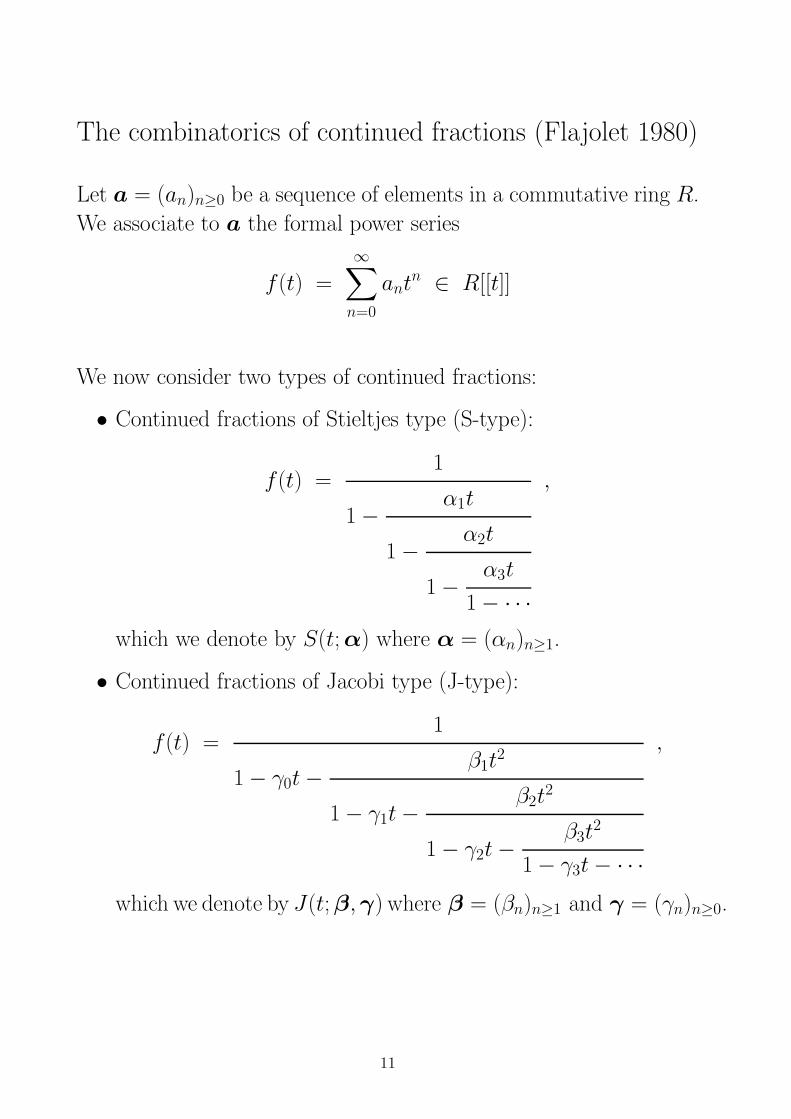
The combinatorics of continued fractions (Flajolet 1980)
Let a = (an)n≥0 be a sequence of elements in a commutative ring R.
We associate to a the formal power series
f(t) =
∞∑
n=0
antn ∈ R[[t]]
We now consider two types of continued fractions:
• Continued fractions of Stieltjes type (S-type):
f(t) =1
1 −α1t
1 −α2t
1 −α3t
1 − · · ·
,
which we denote by S(t; α) where α = (αn)n≥1.
• Continued fractions of Jacobi type (J-type):
f(t) =1
1 − γ0t −β1t
2
1 − γ1t −β2t
2
1 − γ2t −β3t
2
1 − γ3t − · · ·
,
which we denote by J(t; β, γ) where β = (βn)n≥1 and γ = (γn)n≥0.
11

The combinatorics of continued fractions (continued)
Theorem (Flajolet 1980): As an identity in Z[α][[t]], we have
1
1 −α1t
1 −α2t
1 − · · ·
=∞
∑
n=0
Sn(α1, . . . , αn) tn
where Sn(α1, . . . , αn) is the generating polynomial for Dyck paths of
length 2n in which each fall starting at height i gets weight αi.
Sn(α) is called the Stieltjes–Rogers polynomial of order n.
Theorem (Flajolet 1980): As an identity in Z[β, γ][[t]], we have
1
1 − γ0t −β1t
2
1 − γ1t −β2t
2
1 − γ2t − · · ·
=∞
∑
n=0
Jn(β, γ) tn
where Jn(β, γ) is the generating polynomial for Motzkin paths of
length n in which each level step at height i gets weight γi and each
fall starting at height i gets weight βi.
Jn(β, γ) is called the Jacobi–Rogers polynomial of order n.
12

Hankel matrix of Stieltjes–Rogers polynomials
Now form the infinite Hankel matrix corresponding to the sequence
S = (Sn(α))n≥0 of Stieltjes–Rogers polynomials:
H∞(S) =(
Si+j(α))
i,j≥0
And consider any minor of H∞(S):
∆IJ(S) = det HIJ(S)
where I = {i1, i2, . . . , ik} with 0 ≤ i1 < i2 < . . . < ikand J = {j1, j2, . . . , jk} with 0 ≤ j1 < j2 < . . . < jk
Theorem (Viennot 1983): The minor ∆IJ(S) is the generating
polynomial for families of disjoint Dyck paths P1, . . . , Pk where path
Pr starts at (−2ir, 0) and ends at (2jr, 0), in which each fall starting
at height i gets weight αi.
The proof uses the Karlin–McGregor–Lindstrom–Gessel–Viennot lemma
on families of nonintersecting paths.
Corollary: The sequence S = (Sn(α))n≥0 is a Hankel-totally positive
sequence in the polynomial ring Z[α] equipped with the coefficientwise
partial order.
Now specialize α to nonnegative elements in any partially ordered
commutative ring:
Corollary: Let α = (αn)n≥1 be a sequence of nonnegative elements
in a partially ordered commutative ring R. Then (Sn(α))n≥0 is a
Hankel-totally positive sequence in R.
13

Hankel matrix of Stieltjes–Rogers polynomials (continued)
Can also get explicit formulae for the Hankel determinants
∆(m)n (S) = det H
(m)n (S) for small m:
Theorem:
∆(0)n (S) = (α1α2)
n−1(α3α4)n−2 · · · (α2n−3α2n−2)
∆(1)n (S) = αn
1(α2α3)n−1(α4α5)
n−2 · · · (α2n−2α2n−1)
These formulae are classical in the theory of continued fractions,
but Viennot 1983 gives a beautiful combinatorial interpretation.
See also Ishikawa–Tagawa–Zeng 2009 for extensions to m = 2, 3.
14
Hankel matrix of Jacobi–Rogers polynomials
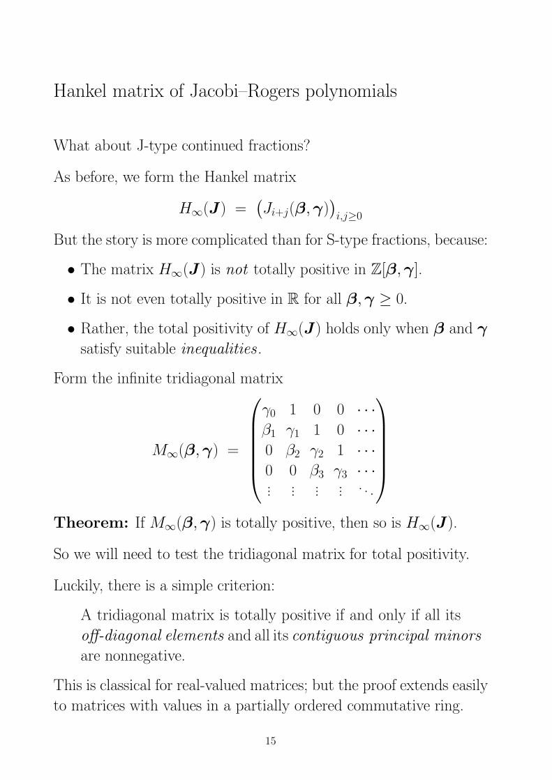
What about J-type continued fractions?
As before, we form the Hankel matrix
H∞(J) =(
Ji+j(β, γ))
i,j≥0
But the story is more complicated than for S-type fractions, because:
• The matrix H∞(J) is not totally positive in Z[β, γ].
• It is not even totally positive in R for all β, γ ≥ 0.
• Rather, the total positivity of H∞(J) holds only when β and γ
satisfy suitable inequalities .
Form the infinite tridiagonal matrix
M∞(β, γ) =
γ0 1 0 0 · · ·β1 γ1 1 0 · · ·0 β2 γ2 1 · · ·0 0 β3 γ3 · · ·... ... ... ... . . .
Theorem: If M∞(β, γ) is totally positive, then so is H∞(J).
So we will need to test the tridiagonal matrix for total positivity.
Luckily, there is a simple criterion:
A tridiagonal matrix is totally positive if and only if all its
off-diagonal elements and all its contiguous principal minors
are nonnegative.
This is classical for real-valued matrices; but the proof extends easily
to matrices with values in a partially ordered commutative ring.
15

Finding Hankel-totally positive sequences of polynomials
A general strategy:
1. Start from a sequence (cn)n≥0 of positive real numbers that is a
Stieltjes moment sequence, i.e. is Hankel-totally positive.
[This property is easy to test empirically: just expand the
generating series∑∞
n=0 cntn as an S-type continued fraction and
test whether all coefficients αi are ≥ 0.]
2. Refine this sequence somehow to a row-finite array (cn,k)0≤k≤kmax(n)
satisfyingkmax(n)
∑
k=0
cn,k = cn;
then define the polynomials Pn(x) =kmax(n)
∑
k=0
cn,k xk.
3. By construction, the sequence (Pn(1))n≥0 is Hankel-totally positive;
and if we are lucky, we will find that two successively stronger
properties of Hankel-total positivity also hold:
(a) For each real number x ≥ 0, the sequence (Pn(x))n≥0 of real
numbers is Hankel-totally positive (i.e. is a Stieltjes moment
sequence).
(b) The sequence (Pn(x))n≥0 of polynomials is coefficientwise
Hankel-totally positive.
• Usually (cn)n≥0 will usually be a sequence of positive integers
having some combinatorial interpretation, i.e. as the cardinality
of some “naturally occurring” set Sn.
• Then the cn,k will arise from the partition of Sn into disjoint
subsets Sn,k according to some “natural” statistic κ : Sn → N.
16

Some examples of combinatorial Stieltjes moment sequences
n Continued fraction0 1 2 3 4 5 6 α2k−1 α2k
Catalan numbers Cn 1 1 2 5 14 42 132 1 1
Central binomials(
2n
n
)
1 2 6 20 70 252 924 α1 = 2, 1
all others 1
Bell numbers Bn 1 1 2 5 15 52 203 1 k
Irreducible Bell numbers IBn+1 1 1 2 6 22 92 426 k 1
Factorials n! 1 1 2 6 24 120 720 k k
Ordered Bell numbers OBn 1 1 3 13 75 541 4683 k 2k
Odd semifactorials (2n − 1)!! 1 1 3 15 105 945 10395 2k − 1 2k
Even semifactorials (2n)!! 1 2 8 48 384 3840 46080 2k 2k
Genocchi medians H2n+1 1 1 2 8 56 608 9440 k2 k2
Genocchi numbers G2n+2 1 1 3 17 155 2073 38227 k2 k(k + 1)
Secant numbers E2n 1 1 5 61 1385 50521 2702765 (2k − 1)2 (2k)2
Tangent numbers E2n+1 1 2 16 272 7936 353792 22368256 (2k−1)(2k) (2k)(2k+1)
So our polynomial examples will divide naturally into “families”:
the Catalan family, the Bell family, the factorial family, etc.
Can also pursue this strategy in reverse:
• Find the S-type continued fraction for the generating series∞∑
n=0cnt
n.
• Generalize it by inserting one or more indeterminates x.
• Try to compute the corresponding polynomials Pn(x) and/or
find a combinatorial interpretation for them.
Caveat:
• There also exist important combinatorial Stieltjes moment sequences
that do not seem to have nice continued fractions.
• Some of them have polynomial refinements that are empirically
Hankel-totally positive; but new methods will be needed to prove it!
17

Example 1: Narayana polynomials
• Narayana numbers N(n, k) =1
n
(
n
k
)(
n
k − 1
)
for n ≥ k ≥ 1
with convention N(0, k) = δk0
• They refine Catalan numbers:n∑
k=0
N(n, k) = Cn
• They count numerous objects of combinatorial interest:
– Dyck paths of length 2n with k peaks
– Non-crossing partitions of [n] with k blocks
– Non-nesting partitions of [n] with k blocks
• Define Narayana polynomials Nn(x) =n∑
k=0
N(n, k) xk
• Define ordinary generating function N (t, x) =∞∑
n=0tn Nn(x)
• Elementary “renewal” argument on Dyck paths implies
N =1
1 − tx − t(N − 1)
which can be rewritten as
N =1
1 −xt
1 − tN
• Leads immediately to S-type continued fraction∞
∑
n=0
tn Nn(x) =1
1 −xt
1 −t
1 −xt
1 −t
1 − · · ·with coefficients α2k−1 = x, α2k = 1.
18

Narayana polynomials (continued)
Conclusions:
1. The sequence N = (Nn(x))n≥0 of Narayana polynomials is
coefficientwise Hankel-totally positive. The minor ∆IJ(N ) counts
families of disjoint Dyck paths as specified by Viennot 1983, with
weights α2k−1 = x, α2k = 1.
2. The first Hankel determinants ∆(m)n (N ) are
∆(0)n (N ) = xn(n−1)/2
∆(1)n (N ) = xn(n+1)/2
Remarks:
1. The strong log-convexity was known previously (Chen–Wang–
Yang 2010), but with a much more difficult proof.
2. The formula for ∆(0)n (N ) was also known (Sivasubramanian 2010),
by an explicit bijective argument.
19

Example 2: Bell polynomials
• Stirling number{
nk
}
= # of partitions of [n] with k blocks
• Convention{
0k
}
= δk0
• They refine Bell numbers:n∑
k=0
{
nk
}
= Bn
• Define Bell polynomials Bn(x) =n∑
k=0
{
nk
}
xk
• Define ordinary generating function B(t, x) =∞∑
n=0tn Bn(x)
• Flajolet (1980) expressed B(t, x) as a J-type continued fraction
• Can be transformed to an S-type continued fraction
∞∑
n=0
tn Bn(x) =1
1 −xt
1 −1t
1 −xt
1 −2t
1 − · · ·
with coefficients α2k−1 = x, α2k = k.
20

Bell polynomials (continued)
Conclusions:
1. The sequence B = (Bn(x))n≥0 of Bell polynomials is
coefficientwise Hankel-totally positive. The minor ∆IJ(B) counts
families of disjoint Dyck paths as specified by Viennot 1983, with
weights α2k−1 = x, α2k = k.
2. The first Hankel determinants ∆(m)n (B) are
∆(0)n (B) = xn(n−1)/2
n−1∏
i=1
i!
∆(1)n (B) = xn(n+1)/2
n−1∏
i=1
i!
Remarks:
1. The strong log-convexity was known previously (Chen–Wang–
Yang 2011).
2. The formula for ∆(0)n (B) has also been known for a long time
(Radoux 1979, Ehrenborg 2000).
3. For each real number x ≥ 0, the sequence (Bn(x))∞n=0 is the
moment sequence for the Poisson distribution of expected value x:
Bn(x) =∞
∑
k=0
kn
(
e−xxk
k!
)
Hence (Bn(x))∞n=0 is a Hankel-totally positive sequence of real
numbers. But the weights e−xxk/k! here are not nonnegative
elements of R[x] or R[[x]], so this approach cannot be used to
prove the coefficientwise total positivity.
21

Example 3: Interpolating between Narayana and Bell
• Let π = {B1, B2, . . . , Bk} be a partition of [n]
• Associate to π a graph Gπ with vertex set [n] such that i, j are
joined by an edge iff they are consecutive elements within the
same block
• Always write an edge e of Gπ as a pair (i, j) with i < j
• We say that edges e1 = (i1, j1) and e2 = (i2, j2) of Gπ form
– a crossing if i1 < i2 < j1 < j2
– a nesting if i1 < i2 < j2 < j1
• We define cr(π) [resp. ne(π)] to be number of crossings
(resp. nestings) in π
• Write |π| = k for the number of blocks in π
• Now define the three-variable polynomial
Bn(x, p, q) =∑
π∈Πn
x|π|pcr(π)qne(π)
with the convention B0(x, p, q) = 1
• Bn(x, 0, 1) = Bn(x, 1, 0) = Nn(x) and Bn(x, 1, 1) = Bn(x),
so this polynomial generalizes the Narayana and Bell polynomials.
• Kasraoui and Zeng (2006) have constructed an involution on
Πn that preserves the number of blocks (as well as some other
properties) and exchanges the numbers of crossings and nestings;
thus Bn(x, p, q) = Bn(x, q, p).
• Define ordinary generating functionB(t, x, p, q) =∞∑
n=0tn Bn(x, p, q)
22

Interpolating between Narayana and Bell (continued)
• Kasraoui and Zeng (2006) have expressed B(t, x, p, q) as a
J-type continued fraction
• Can be transformed to an S-type continued fraction∞
∑
n=0
tn Bn(x, p, q) =1
1 −xt
1 −[1]p,qt
1 −xt
1 −[2]p,qt
1 − · · ·with coefficients α2k−1 = x, α2k = [k]p,q, where
[k]p,q =pk − qk
p − q
Conclusions:
1. The sequence B = (Bn(x, p, q))n≥0 of three-variable polynomials
is coefficientwise Hankel-totally positive. The minor ∆IJ(B)
counts families of disjoint Dyck paths as specified by Viennot
1983, with weights α2k−1 = x, α2k = [k]p,q.
2. The first Hankel determinants ∆(m)n (B) are
∆(0)n (B) = xn(n−1)/2
n−1∏
i=1
[i]p,q!
∆(1)n (B) = xn(n+1)/2
n−1∏
i=1
[i]p,q!
where
[n]p,q! =n
∏
j=1
[j]p,q (0.1)
23

Example 4: Eulerian polynomials
• Eulerian number⟨
nk
⟩
= # of permutations of [n] with k descents
• Convention⟨
0k
⟩
= δk0
• They obviously refine factorials:n∑
k=0
⟨
nk
⟩
= n!
• Define Eulerian polynomials An(x) =n∑
k=0
⟨
nk
⟩
xk
• Define ordinary generating function A(t, x) =∞∑
n=0tn An(x)
• Flajolet (1980) expressed A(t, x) as a J-type continued fraction
• Can be transformed to an S-type continued fraction
∞∑
n=0
tn An(x) =1
1 −t
1 −xt
1 −2t
1 −2xt
1 − · · ·
with coefficients α2k−1 = k, α2k = kx.
24

Eulerian polynomials (continued)
Conclusions:
1. The sequence A = (An(x))n≥0 of Eulerian polynomials is
coefficientwise Hankel-totally positive. The minor ∆IJ(A) counts
families of disjoint Dyck paths as specified by Viennot 1983, with
weights α2k−1 = k, α2k = kx.
2. The first Hankel determinants ∆(m)n (A) are
∆(0)n (B) = xn(n−1)/2
n−1∏
i=1
i!2
∆(1)n (B) = xn(n+1)/2
n−1∏
i=1
i!2
Remarks:
1. The (strong) log-convexity was known previously (Liu–Wang
2007, Zhu 2013).
2. The formula for ∆(0)n (A) was also known (Sivasubramanian 2010),
by an explicit bijective argument.
3. Shin and Zeng (2012) have a p, q-generalization of this S-type
continued fraction =⇒ their polynomials An(x, p, q) form a
coefficientwise (in x, p, q) Hankel-totally positive sequence.
25

Example 5: Narayana polynomials of type B
The polynomials
Wn(x) =n
∑
k=0
(
n
k
)2
xk
arise as
• Coordinator polynomial of the classical root lattice An
• Rank generating function of the lattice of noncrossing partitions
of type B on [n]
I follow Chen–Tang–Wang–Yang 2010 in calling them the Narayana
polynomials of type B .
• There is no S-type continued fraction in the ring of polynomials :
we have
α1, α2, . . . = 1+x,2x
1 + x,
1 + x2
1 + x,
x + x2
1 + x2,
1 + x3
1 + x2,
x + x3
1 + x3,
1 + x4
1 + x3, . . .
• However, there is a nice J-type continued fraction: γn = 1 + x,
β1 = 2x, βn = x for n ≥ 2.
• The corresponding tridiagonal matrix is totally positive.
• Conclusion: The sequence (Wn(x))n≥0 is coefficientwise Hankel-
totally positive.
26

Egecioglu–Redmond–Ryavec polynomials
• A noncrossing graph is a graph whose vertices are points on a
circle and whose edges are non-crossing line segments.
• Noy (1998) showed that the number of noncrossing trees on n+2
vertices in which a specified vertex (say, vertex 1) has degree k + 1 is
T (n, k) =k + 1
n + 1
(
3n − k + 1
n − k
)
=2k + 2
3n − k + 2
(
3n − k + 2
n − k
)
• Egecioglu, Redmond and Ryavec (2001) introduced the polynomials
ERRn(x) =n
∑
k=0
T (n, k) xk
• They showed that, surprisingly, the Hankel determinant ∆(0)n (ERR)
is independent of x:
∆(0)n (ERR) =
n∏
i=1
(
6i−22i
)
2(
4i−12i
)
This is the number of (2n+1)×(2n+1) alternating sign matrices
that are invariant under vertical reflection.
• There is no S-type continued fraction in the ring of polynomials :
we have
α1, α2, . . . = 2 + x,3
2 + x,
11 + 10x
6 + 3x,
52 + 26x
33 + 30x, . . .
• However, there is a J-type continued fraction where γ0 = 2 + x
and all the other coefficients are known numbers.
• The corresponding tridiagonal matrix is totally positive.
• Conclusion: The sequence (ERRn(x))n≥0 is coefficientwise Hankel-
totally positive.
27

Some cases I am unable (as yet) to prove . . .
Finally, there are some cases where I find empirically that a se-
quence (Pn(x))n≥0 is coefficientwise Hankel-totally positive, but I
am unable to prove it because there is neither an S-type nor a J-type
continued fraction in the ring of polynomials:
• Domb polynomials
• Apery polynomials
• Boros–Moll polynomials
• Inversion enumerators for trees
• Reduced binomial discriminant polynomials
...
28
Generating polynomials of connected graphs
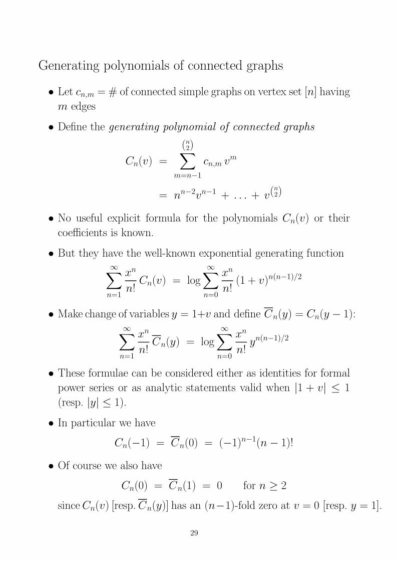
• Let cn,m = # of connected simple graphs on vertex set [n] having
m edges
• Define the generating polynomial of connected graphs
Cn(v) =
(n
2)∑
m=n−1
cn,m vm
= nn−2vn−1 + . . . + v(n
2)
• No useful explicit formula for the polynomials Cn(v) or their
coefficients is known.
• But they have the well-known exponential generating function∞
∑
n=1
xn
n!Cn(v) = log
∞∑
n=0
xn
n!(1 + v)n(n−1)/2
• Make change of variables y = 1+v and define Cn(y) = Cn(y − 1):∞
∑
n=1
xn
n!Cn(y) = log
∞∑
n=0
xn
n!yn(n−1)/2
• These formulae can be considered either as identities for formal
power series or as analytic statements valid when |1 + v| ≤ 1
(resp. |y| ≤ 1).
• In particular we have
Cn(−1) = Cn(0) = (−1)n−1(n − 1)!
• Of course we also have
Cn(0) = Cn(1) = 0 for n ≥ 2
since Cn(v) [resp. Cn(y)] has an (n−1)-fold zero at v = 0 [resp. y = 1].
29

Inversion enumerator for trees
• Let T be a tree with vertex set [n], rooted at the vertex 1.
• An inversion of T is an ordered pair (j, k) of vertices such that
j > k > 1 and the path from 1 to k passes through j.
• Let in,ℓ denote the number of trees on [n] having ℓ inversions.
• Define the inversion enumerator for trees
In(y) =
(n−1
2 )∑
ℓ=0
in,ℓ yℓ
= (n − 1)! + . . . + y(n−1
2 )
• The polynomial In(y) turns out to be related to Cn(v) by the
beautiful formula
Cn(v) = vn−1 In(1 + v)
or equivalently
Cn(y) = (y − 1)n−1 In(y)
• This shows in particular that In(0) = (n−1)! and In(1) = nn−2.
• It is useful to define the normalized polynomials
I⋆n(y) =
In(y)
(n − 1)!
which have nonnegative rational coefficients and constant term 1.
30

Inversion enumerator for trees (continued)
Fact 1. In(y) has strictly positive coefficients.
• Nonnegativity is obvious; strict positivity takes a bit of work.
Fact 2. In(y) has log-concave coefficients.
• Special case of a deep result of Huh, arXiv:1201.2915, on the
log-concavity of the h-vector of the independent-set complex for
matroids representable over a field of characteristic 0: apply it
to M ∗(Kn).
• Open problem: Find an elementary direct proof.
Now form the sequence I = (In+1(y))n≥0.
Conjecture 1. The sequence I is coefficientwise Hankel-totally
positive.
• I have checked this through the 10 × 10 Hankel matrix.
• Even the log-convexity In−1In+1 � I2n seems to be an open problem!
Conjecture 2. The 2 × 2 minors Im−1In+1 − ImIn (1 ≤ m ≤ n)
have coefficients that are log-concave.
• I have checked this through n = 165.
• It is false for minors of size 3 × 3 and higher.
31

Inversion enumerator for trees (continued)
Now look at the normalized polynomials I⋆ = (I⋆n+1(y))n≥0.
Conjecture 3. The sequence I⋆ is coefficientwise Hankel-totally
positive.
• I have checked this through the 10 × 10 Hankel matrix.
• The analogous result for fixed real y ∈ [0, 1] can be proven by
using a result of Laguerre on the real-rootedness of the “deformed
exponential function”
F (x, y) =∞
∑
n=0
xn
n!yn(n−1)/2
This is what led me to conjecture the coefficientwise Hankel-
total positivity.
• At fixed real y, the result for I⋆ implies the one for I, by virtue
of a general fact about Hadamard products. But this argument
does not work in R[y]!
Conjecture 4. All the Hankel minors of I⋆ have coefficients that
are log-concave.
• I have checked this through the 10 × 10 Hankel matrix.
• For the 2 × 2 minors, I have checked it for 1 ≤ m ≤ n ≤ 165.
32

Binomial discriminant polynomials
• Define Fn(x, y) =n
∑
k=0
(
n
k
)
xk yk(k−1)/2
• Can be considered as a “y-deformation” of the binomial (1+x)n.
It is also the Jensen polynomial of the deformed exponential function.
• Now define the binomial discriminant polynomial
Dn(y) = discx Fn(x, y)
• Dn(y) is a polynomial with integer coefficients
• It has degree n(n − 1)2/2 and has first and last terms
Dn(y) = b2n yn(n−1)(n−2)/3 + . . . + (−1)n(n−1)/2nnyn(n−1)2/2
where
bn =n−1∏
k=1
(
n
k
)
=n
∏
k=1
k2k−1−n =
n∏
k=1
kk
n∏
k=1
k!
(does this sequence have any standard name?)
• The first few Dn(y) are:
D0(y) = 1
D1(y) = 1
D2(y) = 4 − 4y
D3(y) = 81y2 − 216y3 + 162y4 + 0y5 − 27y6
D4(y) = 9216y8 − 44032y9 + 76032y10 − 46080y11 − 15360y12
+27648y13 − 4608y14 − 3072y15 + 0y16 + 0y17 + 256y18
...
33

Reduced binomial discriminant polynomials
• Dn(y) has a factor yn(n−1)(n−2)/3 and also a factor (1−y)n(n−1)/2
[coming from the fact that the n roots of Fn(x, y) all coalesce as
y → 1].
• So define the reduced binomial discriminant polynomial
Jn(y) =Dn(y)
yn(n−1)(n−2)/3 (1 − y)n(n−1)/2
• Jn(y) is a polynomial with integer coefficients
• It has degree(
n3
)
and has first and last terms
Jn(y) = b2n + . . . + nny(n
3)
• Jn(1) =n∏
k=1
kk (hyperfactorials)
• The first few Jn(y) are:
J0(y) = 1
J1(y) = 1
J2(y) = 4
J3(y) = 81 + 27y
J4(y) = 9216 + 11264y + 5376y2 + 1536y3 + 256y4
...
Conjecture 1. The coefficients of Jn(y) are nonnegative (in fact,
strictly positive).
Conjecture 2. The coefficients of Jn(y) are log-concave (in fact,
strictly log-concave).
• I have checked these conjectures for n ≤ 44.
• What are the coefficients of Jn(y) counting?
34

Reduced binomial discriminant polynomials (continued)
Now form the sequence J = (Jn(y))n≥0.
Conjecture 3. The sequence J is coefficientwise Hankel-totally
positive.
• In fact, all the Hankel minors of J seem to have coefficients that
are strictly positive .
• I have checked this through the 9 × 9 Hankel matrix.
Conjecture 4. All the Hankel minors of J have coefficients that
are log-concave (in fact, strictly log-concave).
• I have checked this through the 9 × 9 Hankel matrix.
• For the 2 × 2 minors, I have checked it for 1 ≤ m ≤ n ≤ 42.
Now look at the normalized polynomials J⋆ = (J⋆n(y))n≥0.
Conjecture 5. The sequence J⋆ is coefficientwise strongly log-
convex : that is, all the 2 × 2 minors J⋆m−1J
⋆n+1 − J⋆
mJ⋆n have non-
negative coefficients.
• I have checked this for 1 ≤ m ≤ n ≤ 42.
• The 3×3 and higher minors do not have nonnegative coefficients.
Conjecture 6. All the 2×2 minors J⋆m−1J
⋆n+1−J⋆
mJ⋆n have coefficients
that are log-concave (in fact, strictly log-concave except when m=n=1).
• I have checked this for 1 ≤ m ≤ n ≤ 42.
35

(Tentative) Conclusion
• Many interesting sequences (Pn(x))n≥0 of combinatorial polynomials
are (or appear to be) coefficientwise Hankel-totally positive.
• In some cases this can be proven by the Flajolet–Viennot method
of continued fractions.
– Flajolet and Viennot emphasized J-type continued fractions
because they are more general.
– But S-type continued fractions, when they exist, often have
simpler coefficients; and they are the most direct tool for
proving Hankel-total positivity.
– Roughly speaking:
J-type c.f. ⇐⇒ general orthogonal polynomials ⇐⇒ Hamburger moment problem
S-type c.f. ⇐⇒ orthogonal polynomials on [0,∞) ⇐⇒ Stieltjes moment problem⇐⇒ Hankel-total positivity
– But sometimes J-type continued fractions exist when S-type
don’t, and they can be used to prove coefficientwise Hankel-
total positivity.
• For the other cases, new methods of proof will be needed.
• Deepest cases seem to be In(y) and Jn(y):
– For In(y), even the log-convexity In−1In+1 � I2n is an open
problem. (Bijective proof??)
– For Jn(y), even the nonnegativity Jn � 0 is an open problem!
We really need to know what Jn(y) is counting!
Dedicated to the memory of Philippe Flajolet
36