COEN 6521 VLSI Testing:Built-In Self Test

Zeljko Zilic(In Ottawa)

zeljko@ece.mcgill.ca

Some slides based on the material provided by Bushnell and Agrawal

Overview

Introduction to BISTTest Pattern GeneratorsResponse Compactors

Economics of BIST - Complexity

ComplexityCascaded devices

No simple way to obtain test vectors for the whole circuit even if tests for individual sub-blocks are given– Tests resulting in 100% fault coverage of individual elements

do not guarantee 100% of the whole design: connections often untestable

BIST allows hierarchical decomposition of cascaded devices for test purposes– Example - Board with few chips: For the chip test system sends

control signal to the board activating BIST on chip. Results aresent back to the system. In case of errors BIST hardware indicates which chip was defective. BIST tests all the embedded designs and interconnects, leaving only functional verification of the cascaded design to system-level tests.

Economic of BIST - TestingTest generation

Practically impossible to carry tests and responses involving hundreds of chip inputs through many layers of circuitry to chip-under-test. BIST localizes testing eliminating these problems

Test applicationBIST saves significantly test application time compared to external testersBIST testing capabilities grow with the VLSI technology, whereas test capabilities always lag behind VLSI technology for external testingLow development cost, as BIST is added to circuits automatically through CAD tools

Cost of BISTChip area overhead for:

Test controllerHardware pattern generatorHardware response compacterTesting of BIST hardware

Pin overhead -- At least 1 pin needed to activate BIST operationPerformance overhead – extra path delays due to BISTYield loss – due to increased chip area or more chips in system because of BISTReliability reduction – due to increased areaIncreased BIST hardware complexity – happens when BIST hardware is made testable

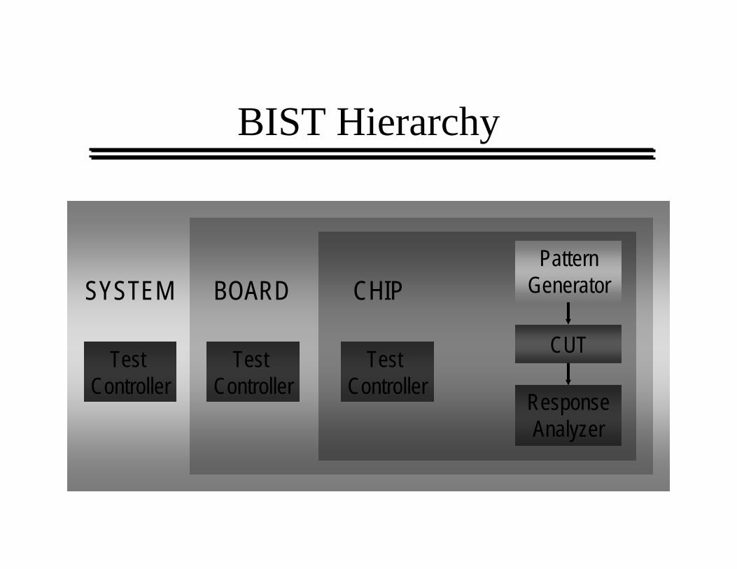
Test Controller

SYSTEM

Test Controller

BOARD

BIST Hierarchy

Test Controller

PatternGenerator

ResponseAnalyzer

CUT

CHIP

Random Logic BIST – Defs. 1

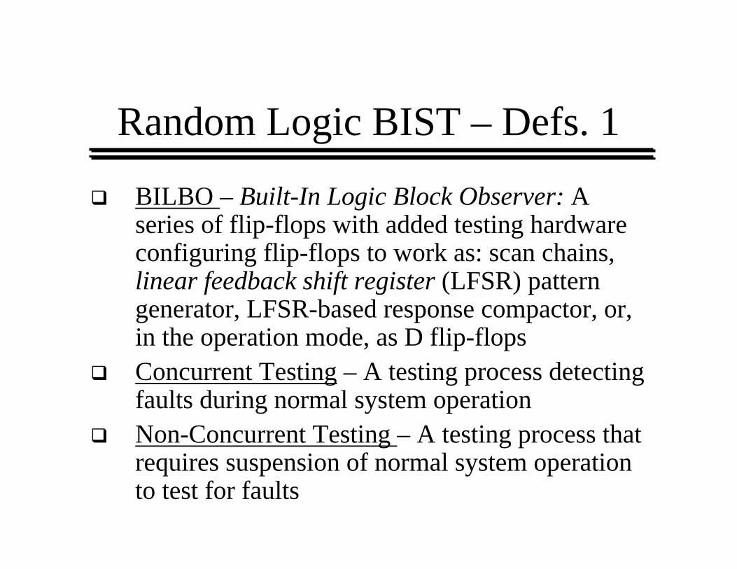
BILBO – Built-In Logic Block Observer: A series of flip-flops with added testing hardware configuring flip-flops to work as: scan chains, linear feedback shift register (LFSR) pattern generator, LFSR-based response compactor, or, in the operation mode, as D flip-flopsConcurrent Testing – A testing process detecting faults during normal system operationNon-Concurrent Testing – A testing process that requires suspension of normal system operation to test for faults

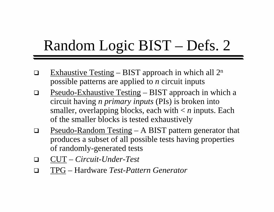
Random Logic BIST – Defs. 2Exhaustive Testing – BIST approach in which all 2n

possible patterns are applied to n circuit inputsPseudo-Exhaustive Testing – BIST approach in which a circuit having n primary inputs (PIs) is broken into smaller, overlapping blocks, each with < n inputs. Each of the smaller blocks is tested exhaustivelyPseudo-Random Testing – A BIST pattern generator that produces a subset of all possible tests having properties of randomly-generated testsCUT – Circuit-Under-TestTPG – Hardware Test-Pattern Generator

Random Logic BIST – Defs. 3

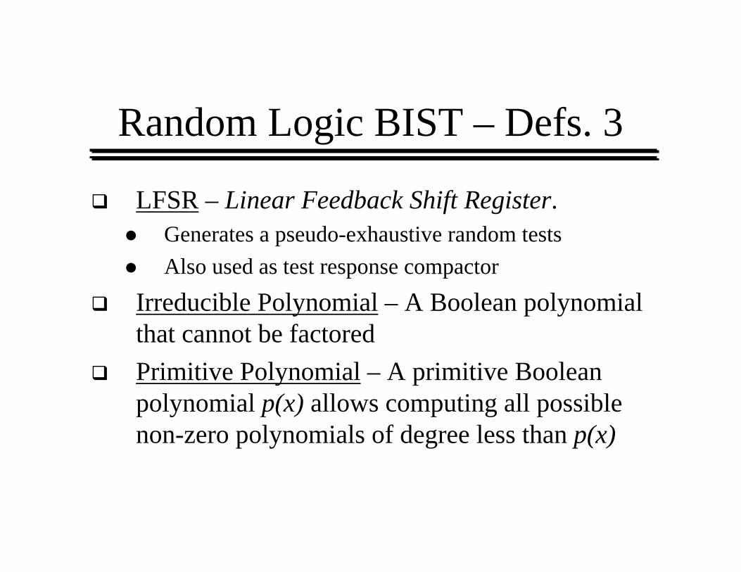
LFSR – Linear Feedback Shift Register. Generates a pseudo-exhaustive random tests Also used as test response compactor

Irreducible Polynomial – A Boolean polynomial that cannot be factoredPrimitive Polynomial – A primitive Boolean polynomial p(x) allows computing all possible non-zero polynomials of degree less than p(x)

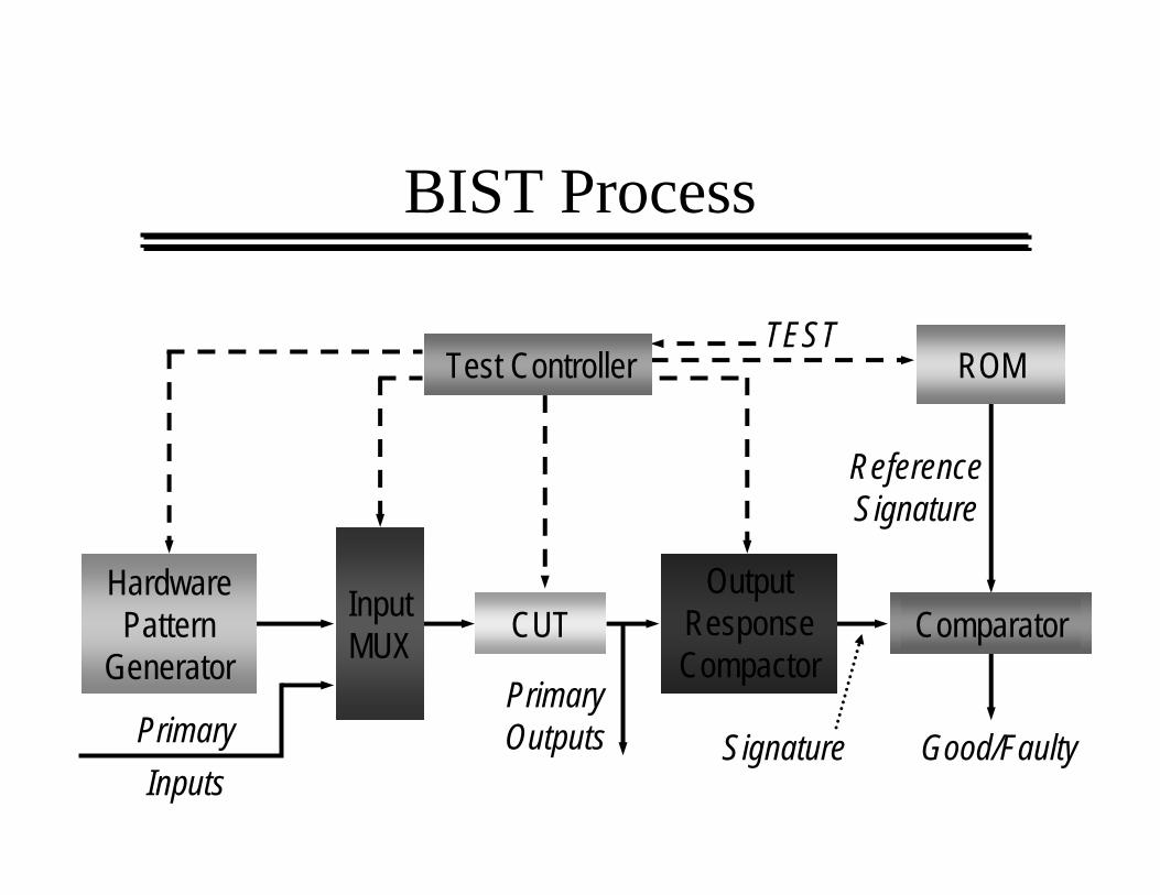
BIST Process

PrimaryInputs

PrimaryOutputs Signature Good/Faulty

ReferenceSignature

TEST

HardwarePattern

Generator

InputMUX CUT

OutputResponseCompactor

Comparator

Test Controller ROM

BIST Controllers

Test controller – Hardware used to activate self-test simultaneously on all PCBsEach board controller activates parallel chip BIST Diagnosis effective only if very high fault coverage

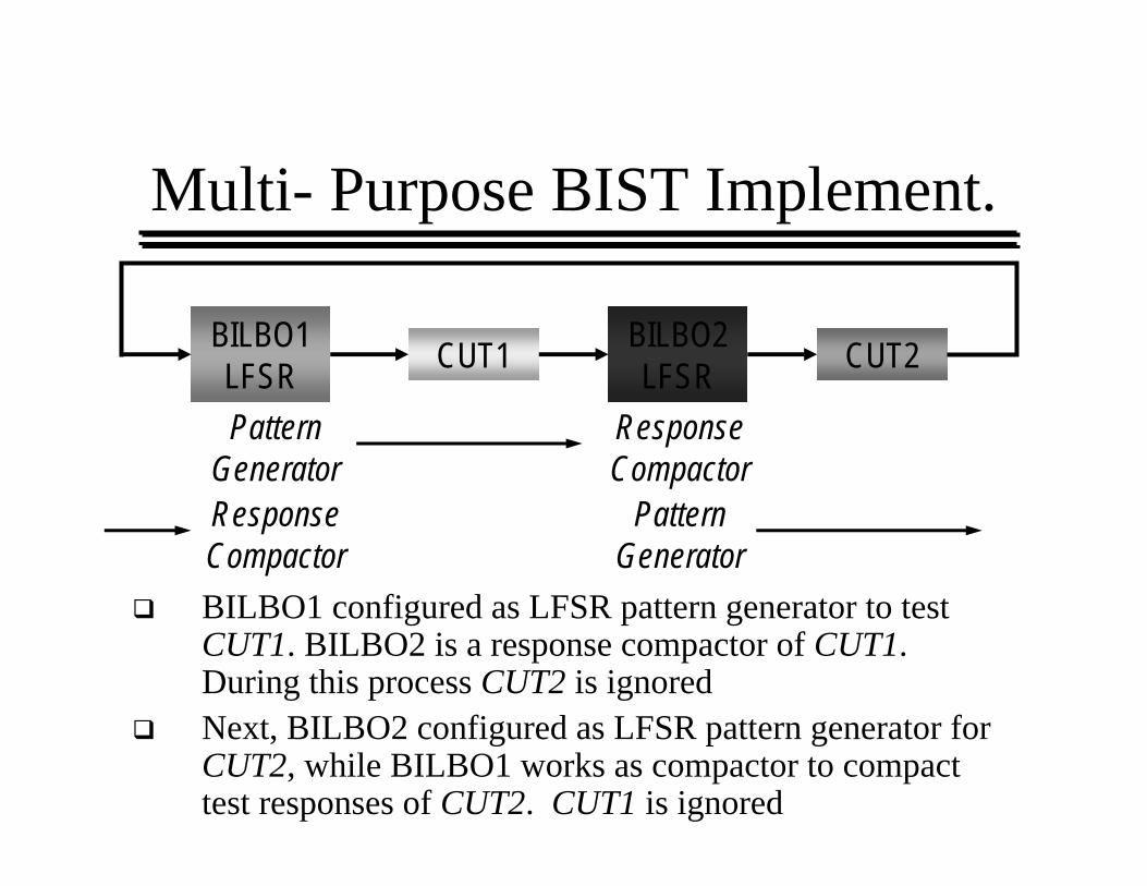
Multi- Purpose BIST Implement.

BILBO1 configured as LFSR pattern generator to test CUT1. BILBO2 is a response compactor of CUT1. During this process CUT2 is ignoredNext, BILBO2 configured as LFSR pattern generator for CUT2, while BILBO1 works as compactor to compact test responses of CUT2. CUT1 is ignored

PatternGenerator

ResponseCompactor

BILBO1LFSR CUT1 BILBO2

LFSR CUT2

PatternGenerator

ResponseCompactor

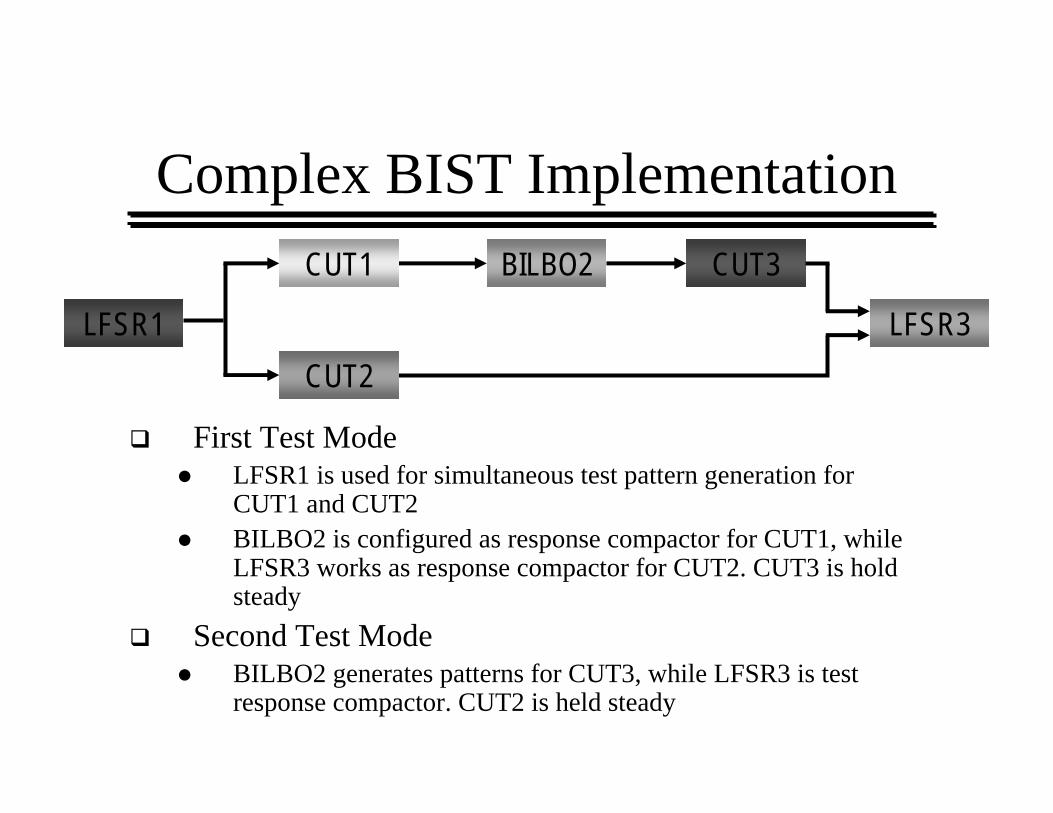
Complex BIST Implementation

First Test ModeLFSR1 is used for simultaneous test pattern generation for CUT1 and CUT2BILBO2 is configured as response compactor for CUT1, while LFSR3 works as response compactor for CUT2. CUT3 is hold steady

Second Test ModeBILBO2 generates patterns for CUT3, while LFSR3 is test response compactor. CUT2 is held steady

CUT1 CUT3BILBO2

LFSR3LFSR1CUT2

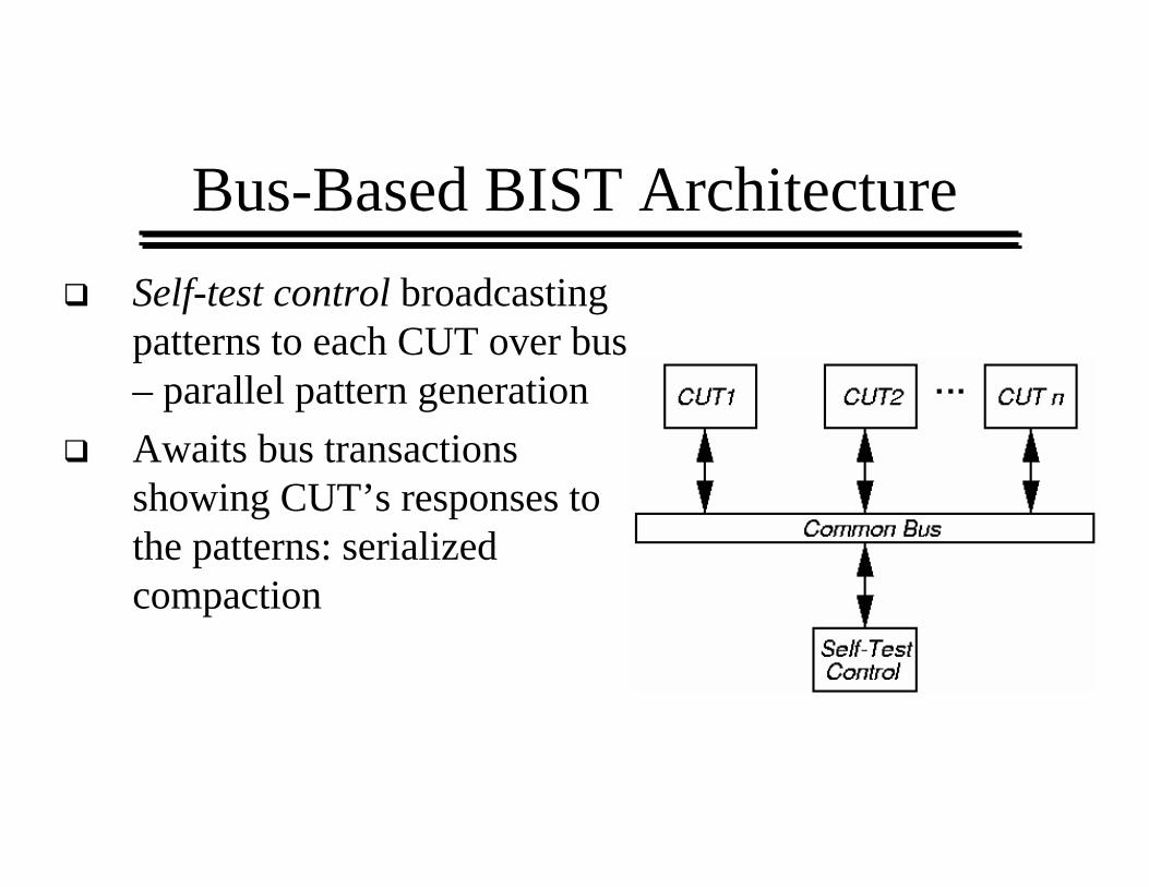
Bus-Based BIST ArchitectureSelf-test control broadcasting patterns to each CUT over bus – parallel pattern generationAwaits bus transactions showing CUT’s responses to the patterns: serialized compaction

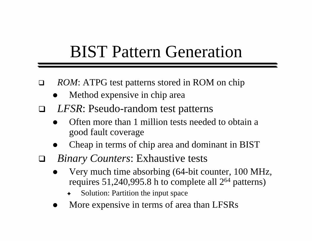
BIST Pattern GenerationROM: ATPG test patterns stored in ROM on chip

Method expensive in chip areaLFSR: Pseudo-random test patterns

Often more than 1 million tests needed to obtain a good fault coverageCheap in terms of chip area and dominant in BIST

Binary Counters: Exhaustive tests Very much time absorbing (64-bit counter, 100 MHz, requires 51,240,995.8 h to complete all 264 patterns)

Solution: Partition the input spaceMore expensive in terms of area than LFSRs

BIST Pattern Generation cont.

LFSR and ROM: LFSR used as the primary test mode. Process augmented with ATPG patterns stored in on chip ROM, which are missing from LFSR sequenceCellular Automata: Each pattern generation cell has few gates, a flip-flop and is connected only to the neighboring gates. The cell is replicated to produce the cellular automata

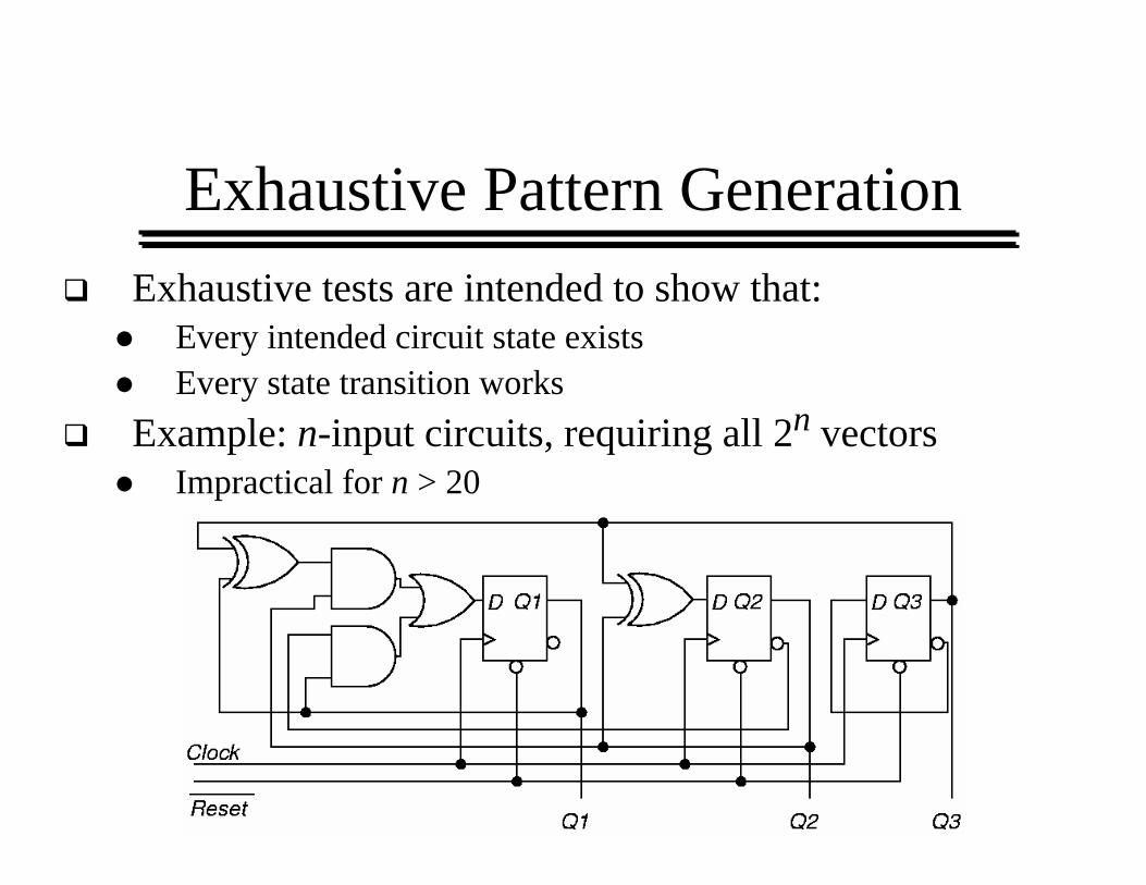
Exhaustive Pattern GenerationExhaustive tests are intended to show that:

Every intended circuit state existsEvery state transition works

Example: n-input circuits, requiring all 2n vectorsImpractical for n > 20

Pseudo-Exhaustive Patterns 1

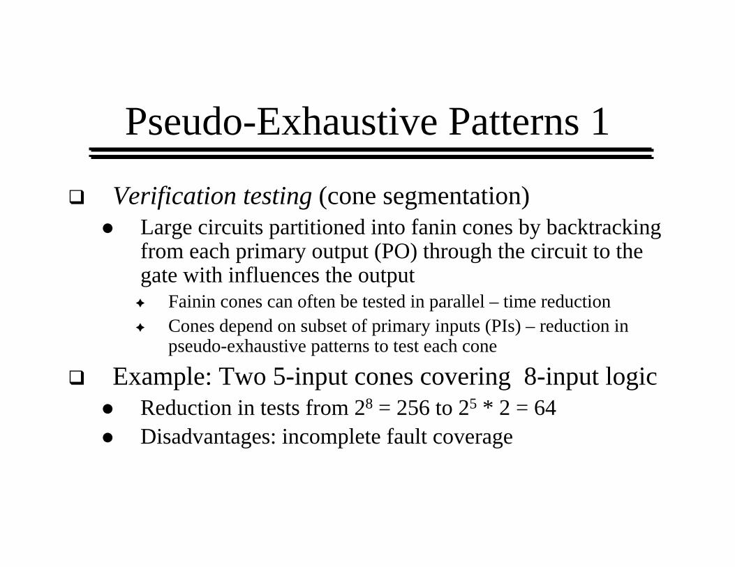
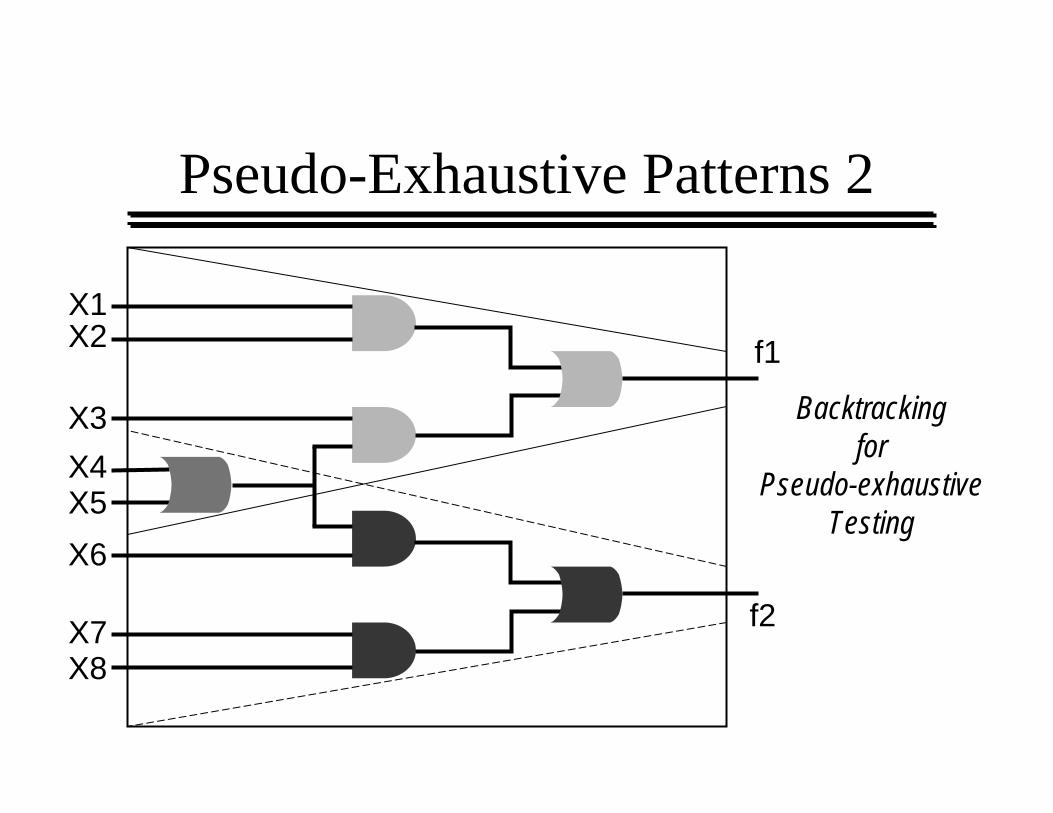
Verification testing (cone segmentation)Large circuits partitioned into fanin cones by backtracking from each primary output (PO) through the circuit to the gate with influences the output

Fainin cones can often be tested in parallel – time reduction Cones depend on subset of primary inputs (PIs) – reduction in pseudo-exhaustive patterns to test each cone

Example: Two 5-input cones covering 8-input logicReduction in tests from 28 = 256 to 25 * 2 = 64Disadvantages: incomplete fault coverage

Pseudo-Exhaustive Patterns 2

X1X1X2X2

X3X3X4X4X5X5

X6X6

X7X7X8X8

f1f1

f2f2

Backtrackingfor

Pseudo-exhaustiveTesting

Pseudo-Exhaustive Patterns 3

Hardware partitioningPhysical segmentation in which extra logic is added to the circuit in order to divide CUT into smaller subcircuits, each subcircuit directly controllable and observable

Each subcircuit tested exhaustively

Sensitized path segmentationCircuit is partitioned so that sensitizing paths are set up from PIs to the partition inputs, and then from the partition outputs to Pos

Each partition is tested individually

Random Pattern Testing

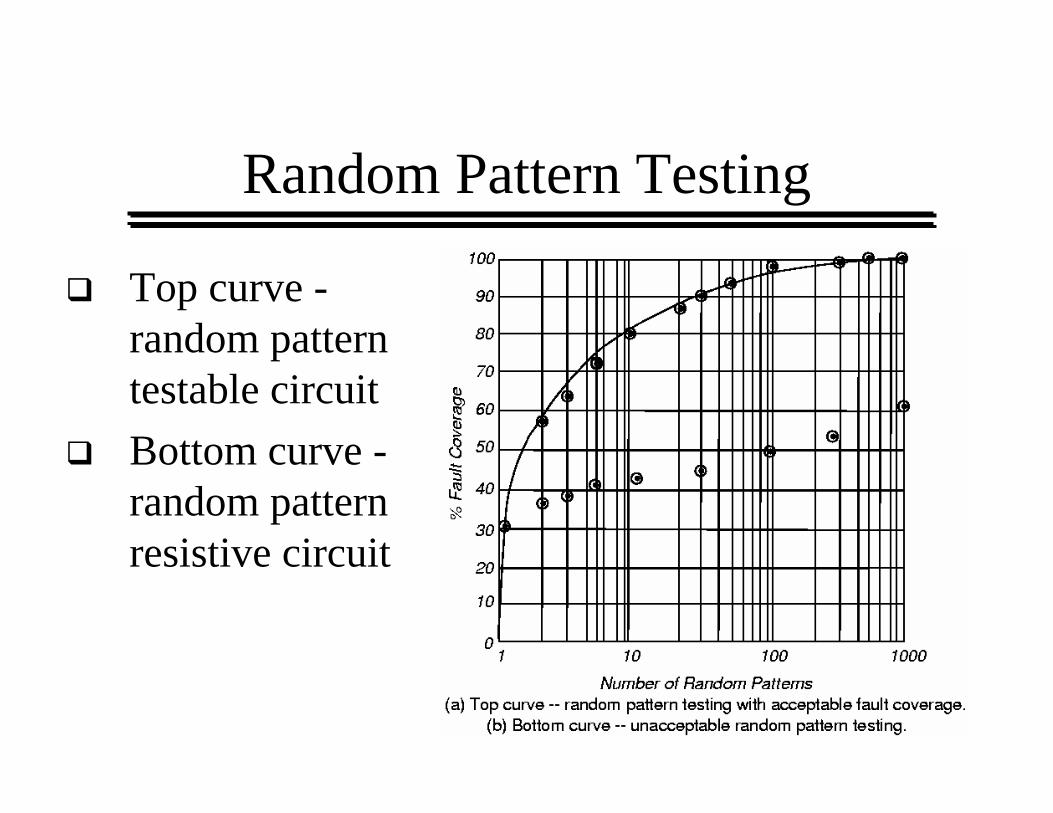
Top curve -random pattern testable circuit Bottom curve -random pattern resistive circuit

Pseudo-Random Pattern Generation

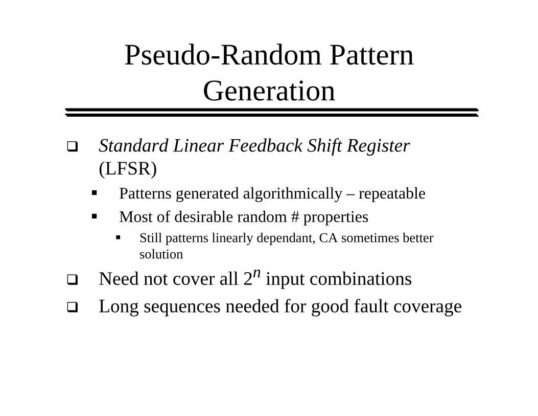
Standard Linear Feedback Shift Register(LFSR)

Patterns generated algorithmically – repeatableMost of desirable random # properties

Still patterns linearly dependant, CA sometimes better solution

Need not cover all 2n input combinationsLong sequences needed for good fault coverage

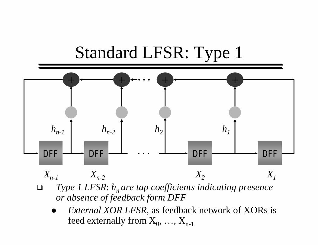
Standard LFSR: Type 1

Type 1 LFSR: hn are tap coefficients indicating presence or absence of feedback form DFF

External XOR LFSR, as feedback network of XORs is feed externally from X0, …, Xn-1

+ + + +

DFF DFF DFF DFF. . .

…

hn-1 hn-2 h2 h1

Xn-1 Xn-2 X2 X1

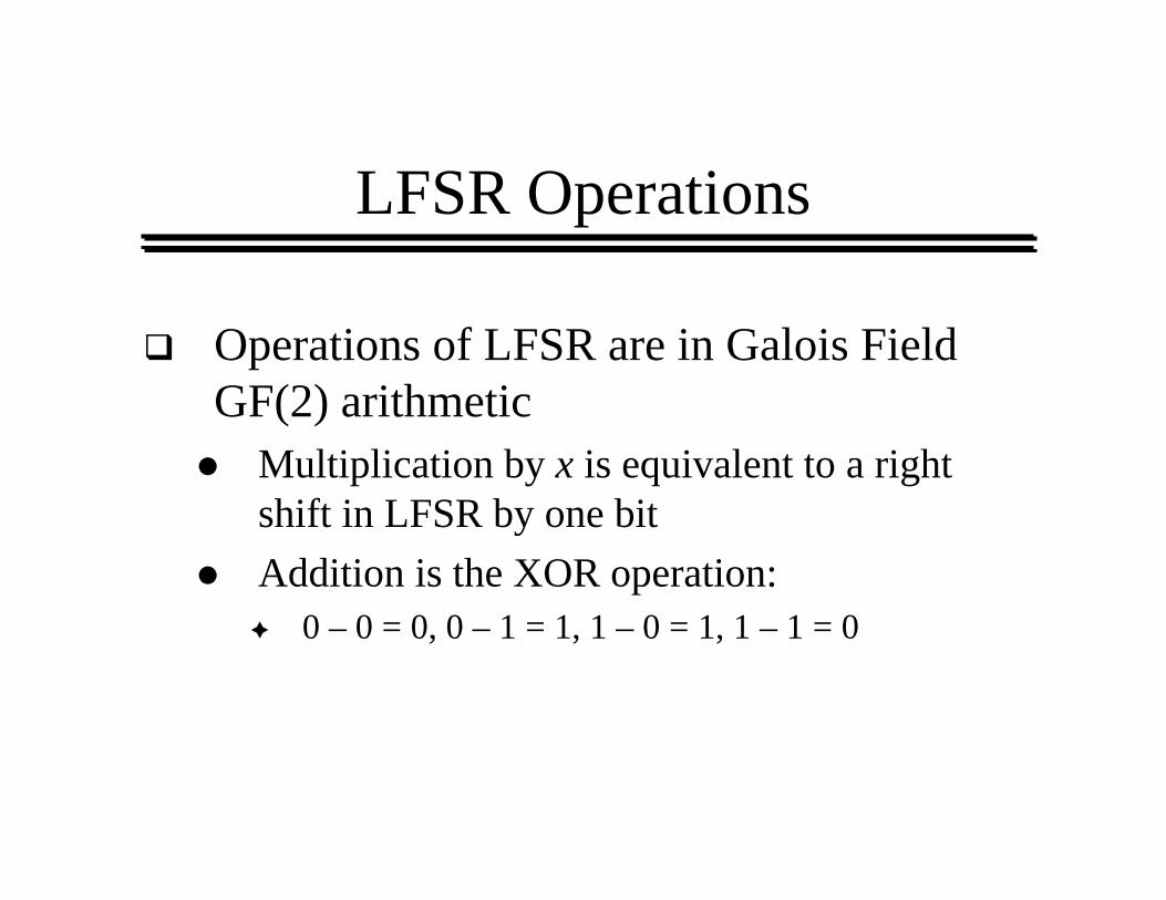
LFSR Operations

Operations of LFSR are in Galois Field GF(2) arithmetic

Multiplication by x is equivalent to a right shift in LFSR by one bitAddition is the XOR operation:

0 – 0 = 0, 0 – 1 = 1, 1 – 0 = 1, 1 – 1 = 0

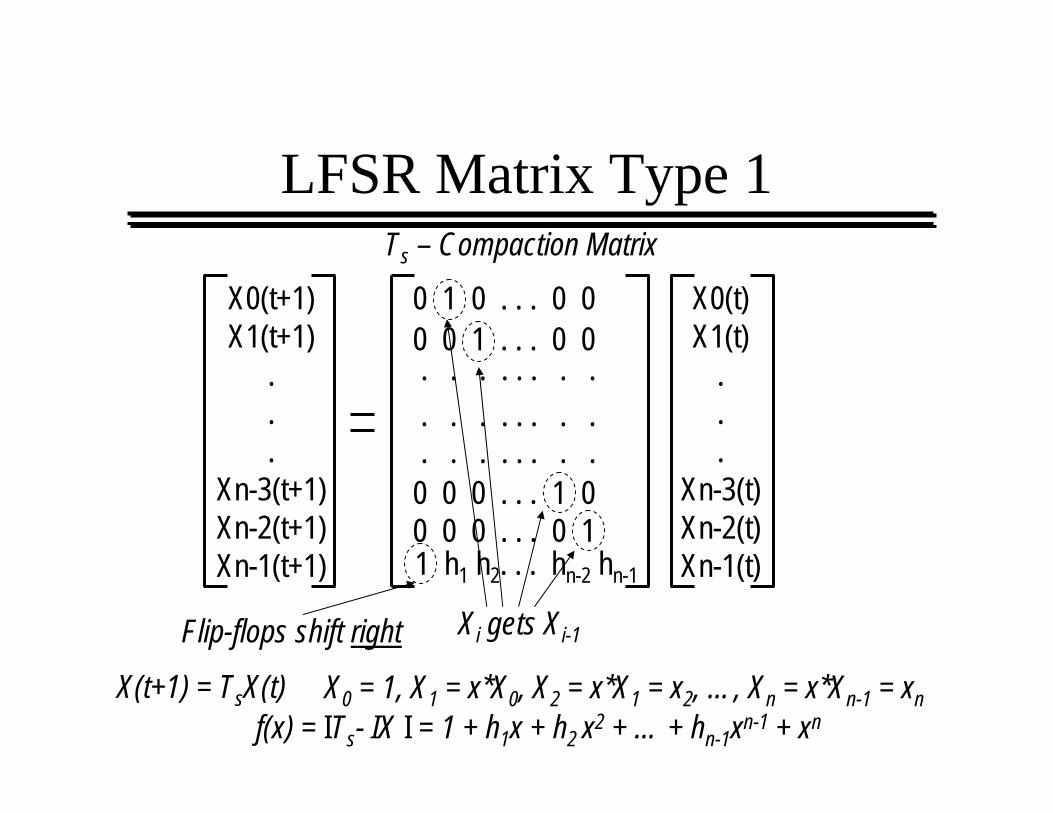
LFSR Matrix Type 1

X0(t+1)X1(t+1)

.

.

.Xn-3(t+1)Xn-2(t+1)Xn-1(t+1)

X0(t)X1(t)

.

.

.Xn-3(t)Xn-2(t)Xn-1(t)

0 1 0 . . . 0 00 0 1 . . . 0 0. . . . . . . .

0 0 0 . . . 1 00 0 0 . . . 0 1

. . . . . . . .

. . . . . . . .

1 h1 h2. . . hn-2 hn-1

Ts – Compaction Matrix

Flip-flops shift right Xi gets Xi-1

X(t+1) = TsX(t) X0 = 1, X1 = x*X0, X2 = x*X1 = x2, …, Xn = x*Xn-1 = xnf(x) = ITs- IX I = 1 + h1x + h2 x2 + … + hn-1xn-1 + xn

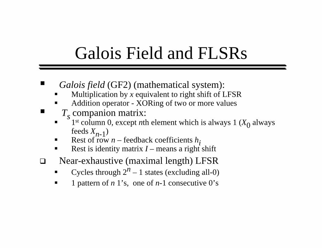
Galois Field and FLSRsGalois field (GF2) (mathematical system):

Multiplication by x equivalent to right shift of LFSRAddition operator - XORing of two or more values

Ts companion matrix:1st column 0, except nth element which is always 1 (X0 always feeds Xn-1)Rest of row n – feedback coefficients hiRest is identity matrix I – means a right shift

Near-exhaustive (maximal length) LFSRCycles through 2n – 1 states (excluding all-0)1 pattern of n 1’s, one of n-1 consecutive 0’s

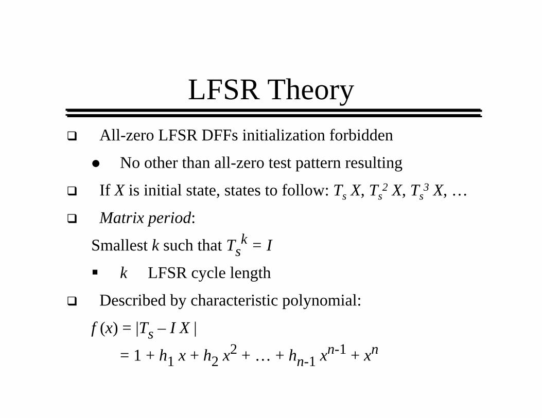
LFSR TheoryAll-zero LFSR DFFs initialization forbidden

No other than all-zero test pattern resulting

If X is initial state, states to follow: Ts X, Ts2 X, Ts

3 X, …

Matrix period:

Smallest k such that Tsk = I

k LFSR cycle length

Described by characteristic polynomial:

f (x) = |Ts – I X |

= 1 + h1 x + h2 x2 + … + hn-1 xn-1 + xn

Maximum-lengths Sequences

There is one pattern of n consecutive ones and one pattern of n-1 consecutive zerosThere is an autocorrelation property

Any two sequences, the original and the circularly shifted sequence (in the same LFSR) will be identical on 2n-1 positions

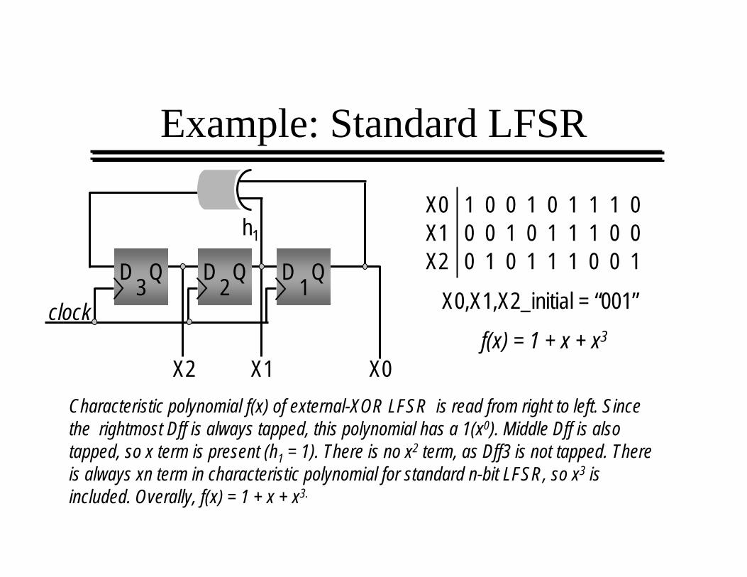
Example: Standard LFSR

D Q D Q D Q

clock

h1

123

X0X1X2f(x) = 1 + x + x3

X0 1 0 0 1 0 1 1 1 0X1 0 0 1 0 1 1 1 0 0X2 0 1 0 1 1 1 0 0 1

X0,X1,X2_initial = “001”

Characteristic polynomial f(x) of external-XOR LFSR is read from right to left. Since the rightmost Dff is always tapped, this polynomial has a 1(x0). Middle Dff is also tapped, so x term is present (h1 = 1). There is no x2 term, as Dff3 is not tapped. There is always xn term in characteristic polynomial for standard n-bit LFSR, so x3 is included. Overally, f(x) = 1 + x + x3.

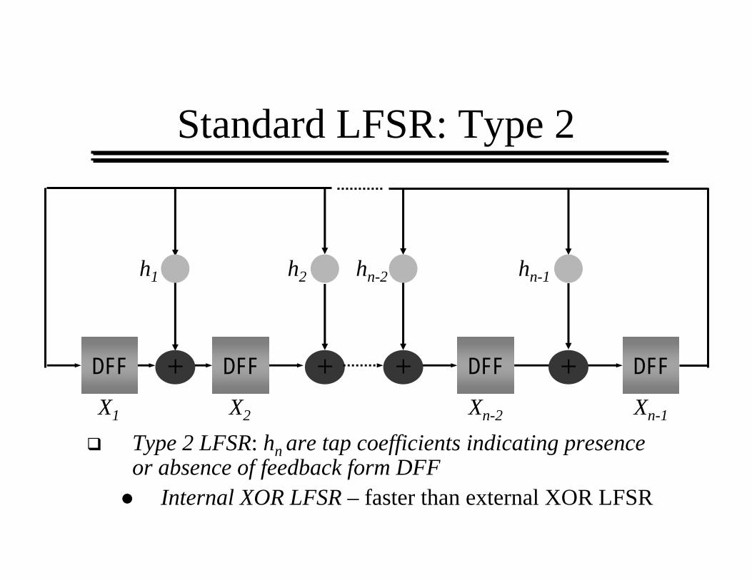
Standard LFSR: Type 2

Type 2 LFSR: hn are tap coefficients indicating presence or absence of feedback form DFF

Internal XOR LFSR – faster than external XOR LFSR

hn-1

DFF DFF DFF

hn-2h2h1

Xn-1Xn-2X2X1

DFF + + + +

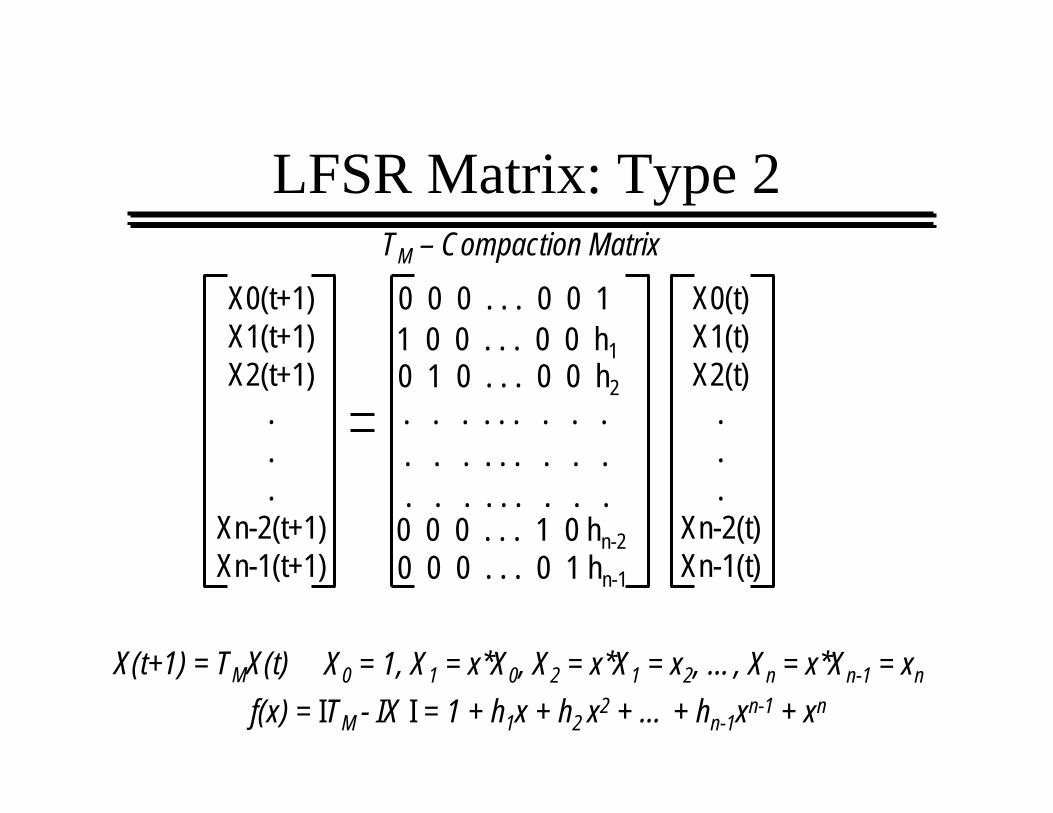
LFSR Matrix: Type 2

X0(t+1)X1(t+1)X2(t+1)

.

.

.Xn-2(t+1)Xn-1(t+1)

X0(t)X1(t)X2(t)

.

.

.Xn-2(t)Xn-1(t)

0 0 0 . . . 0 0 11 0 0 . . . 0 0 h1

. . . . . . . . .

0 0 0 . . . 1 0 hn-20 0 0 . . . 0 1 hn-1

TM – Compaction Matrix

X(t+1) = TMX(t) X0 = 1, X1 = x*X0, X2 = x*X1 = x2, …, Xn = x*Xn-1 = xn

f(x) = ITM - IX I = 1 + h1x + h2 x2 + … + hn-1xn-1 + xn

0 1 0 . . . 0 0 h2

. . . . . . . . .

. . . . . . . . .

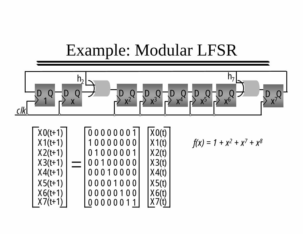
Example: Modular LFSR

clk

D Qh2

1D Q D Q D Q D Q D Q D Q D Q

x x2 x3 x4 x5 x6 x7

h7

0 0 0 0 0 0 0 11 0 0 0 0 0 0 00 1 0 0 0 0 0 10 0 1 0 0 0 0 00 0 0 1 0 0 0 00 0 0 0 1 0 0 00 0 0 0 0 1 0 00 0 0 0 0 0 1 1

X0(t+1)X1(t+1)X2(t+1)X3(t+1)X4(t+1)X5(t+1)X6(t+1)X7(t+1)

X0(t)X1(t)X2(t)X3(t)X4(t)X5(t)X6(t)X7(t)

f(x) = 1 + x2 + x7 + x8

Primitive PolynomialsHighly desirable that LFSR generate all possible 2n-1 patterns (implement primitive polynomials)Requirements for primitive polynomials:

Polynomial must be monic,i.e., coefficient of the highest-order x term of characteristic polynomial must be 1

Modular LFSRs: All Dffs must right shift through XORsfrom X0 to Xn-1, which must then feed back directly to X0Standard LFSRs: All Dffs must right shift from Xn-1 to X0, which must then feed back inot Xn-1 through XORingfeedback network

Characteristic polynomial must divide the polynomial 1+xk for k = 2n – 1, but not for any smaller k

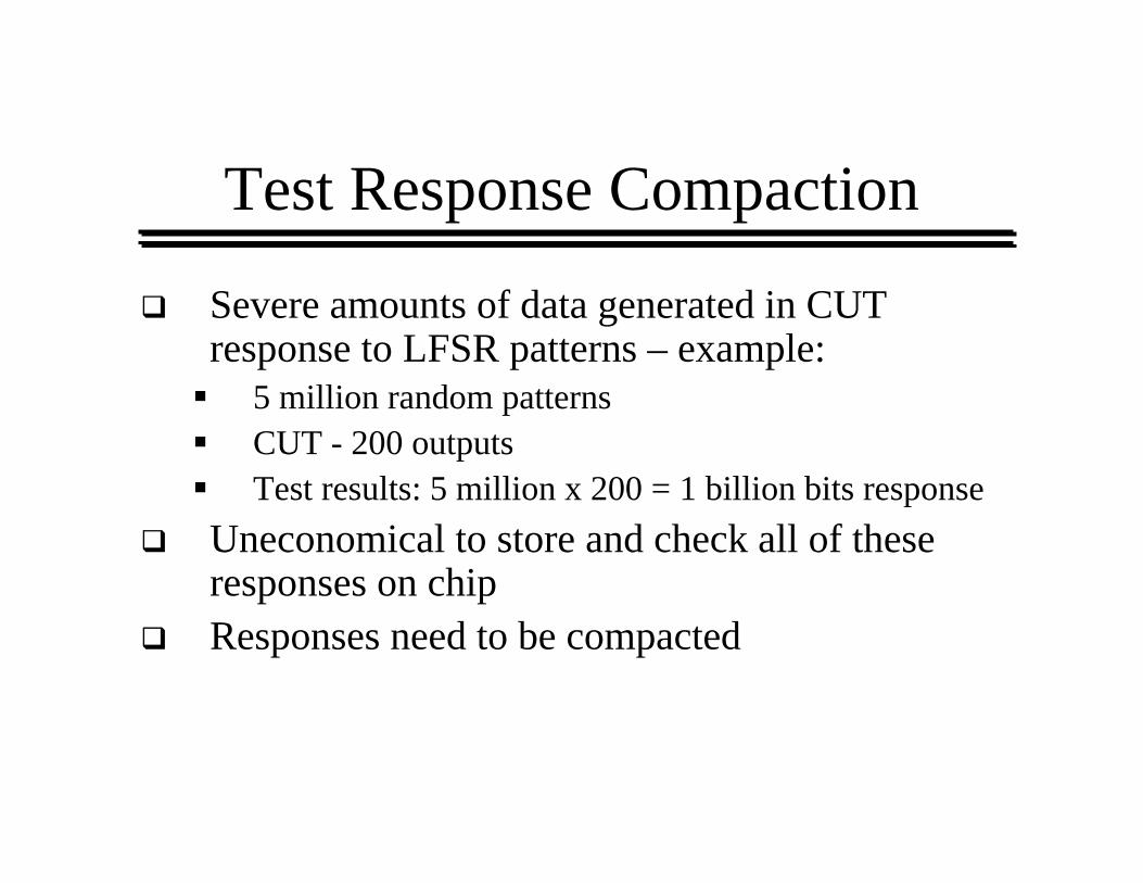
Test Response Compaction

Severe amounts of data generated in CUT response to LFSR patterns – example:

5 million random patternsCUT - 200 outputsTest results: 5 million x 200 = 1 billion bits response

Uneconomical to store and check all of these responses on chipResponses need to be compacted

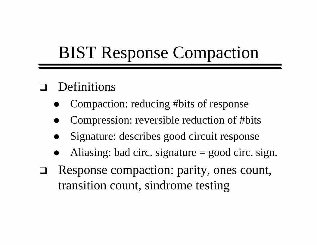
BIST Response Compaction

DefinitionsCompaction: reducing #bits of responseCompression: reversible reduction of #bitsSignature: describes good circuit responseAliasing: bad circ. signature = good circ. sign.

Response compaction: parity, ones count, transition count, sindrome testing

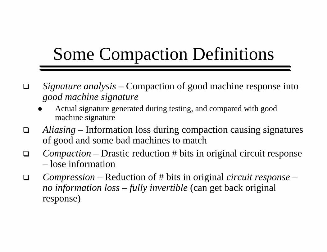
Some Compaction DefinitionsSignature analysis – Compaction of good machine response into good machine signature

Actual signature generated during testing, and compared with good machine signature

Aliasing – Information loss during compaction causing signatures of good and some bad machines to matchCompaction – Drastic reduction # bits in original circuit response – lose informationCompression – Reduction of # bits in original circuit response –no information loss – fully invertible (can get back original response)

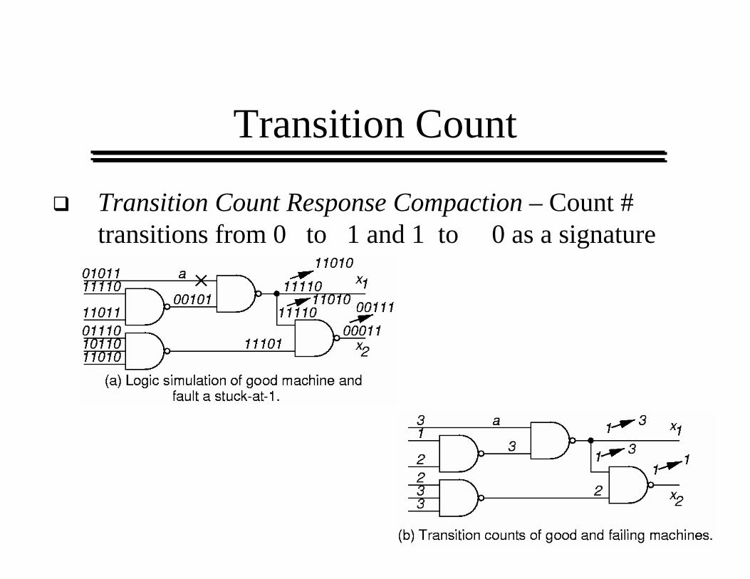
Transition Count

Transition Count Response Compaction – Count # transitions from 0 to 1 and 1 to 0 as a signature

LFSR Response Compaction

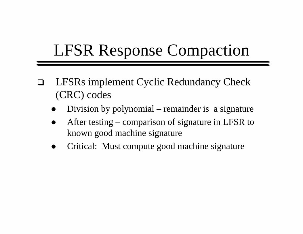
LFSRs implement Cyclic Redundancy Check (CRC) codes

Division by polynomial – remainder is a signatureAfter testing – comparison of signature in LFSR to known good machine signatureCritical: Must compute good machine signature

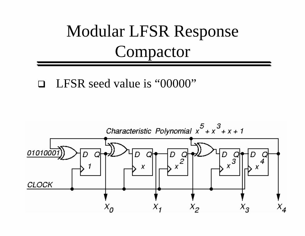
Modular LFSR Response Compactor

LFSR seed value is “00000”

Modular LFSR Compactors - a Good Choice?

Problem with ordinary LFSR response compacter:

Too much hardware if one of these put on each primary output (PO)

Solution: MISR – compacts all outputs into one LFSR

Works because LFSR is linear – obeys superposition principleSuperimpose all responses in one LFSR – final remainder is XOR sum of remainders of polynomial divisions of each PO by the characteristic polynomial

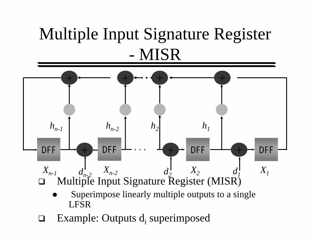
Multiple Input Signature Register - MISR

Multiple Input Signature Register (MISR)Superimpose linearly multiple outputs to a single LFSR

Example: Outputs di superimposed

+ + + +

DFF . . .

…

hn-1 hn-2 h2 h1

Xn-1 Xn-2 X2 X1

+ DFF + DFF+ DFF

dn-2 d2 d1

Aliasing

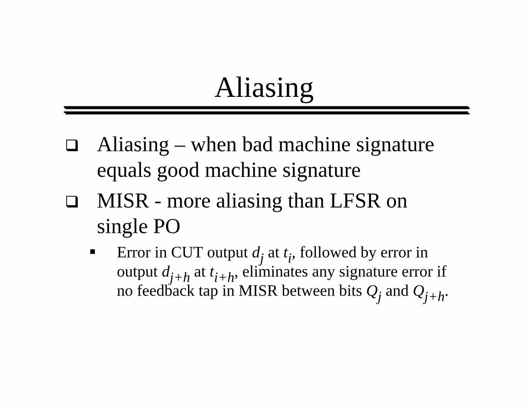
Aliasing – when bad machine signature equals good machine signatureMISR - more aliasing than LFSR on single PO

Error in CUT output dj at ti, followed by error in output dj+h at ti+h, eliminates any signature error if no feedback tap in MISR between bits Qj and Qj+h.

Aliasing Theorems

Theorem 15.1: Assuming that each circuit PO dijhas probability p of being in error, and that all outputs dij are independent, in a k-bit MISR, Pal = 1/(2k), regardless of initial condition of MISR

Not exactly true – true in practice

Aliasing Theorems, cont.

Theorem 15.2: Assuming that each PO dij has

probability pj of being in error, where the pjprobabilities are independent, and that all outputs dij are independent, in a k-bit MISR, Pal = 1/(2k), regardless of the initial condition

Built-in Logic Block Observer

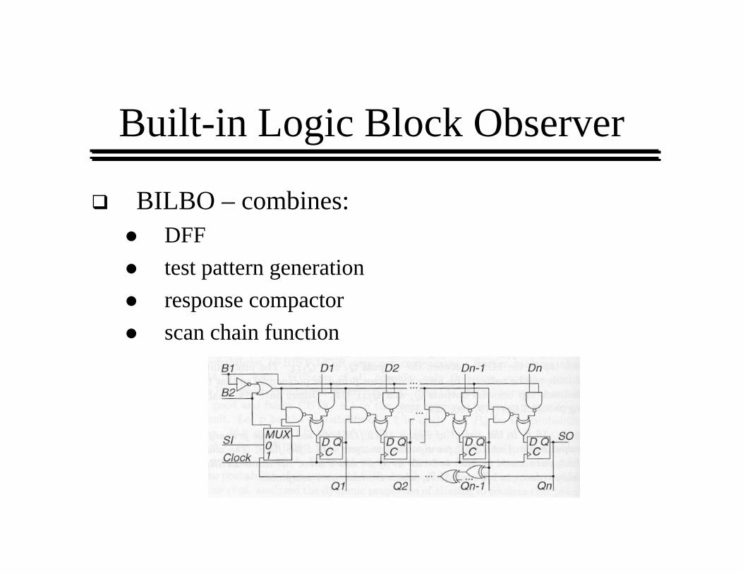
BILBO – combines:DFF test pattern generation response compactorscan chain function

Other BIST Techniques

Test Point InsertionMemory BISTComplex Systems – Networking etc.Delay Fault BISTMixed-signal BIST