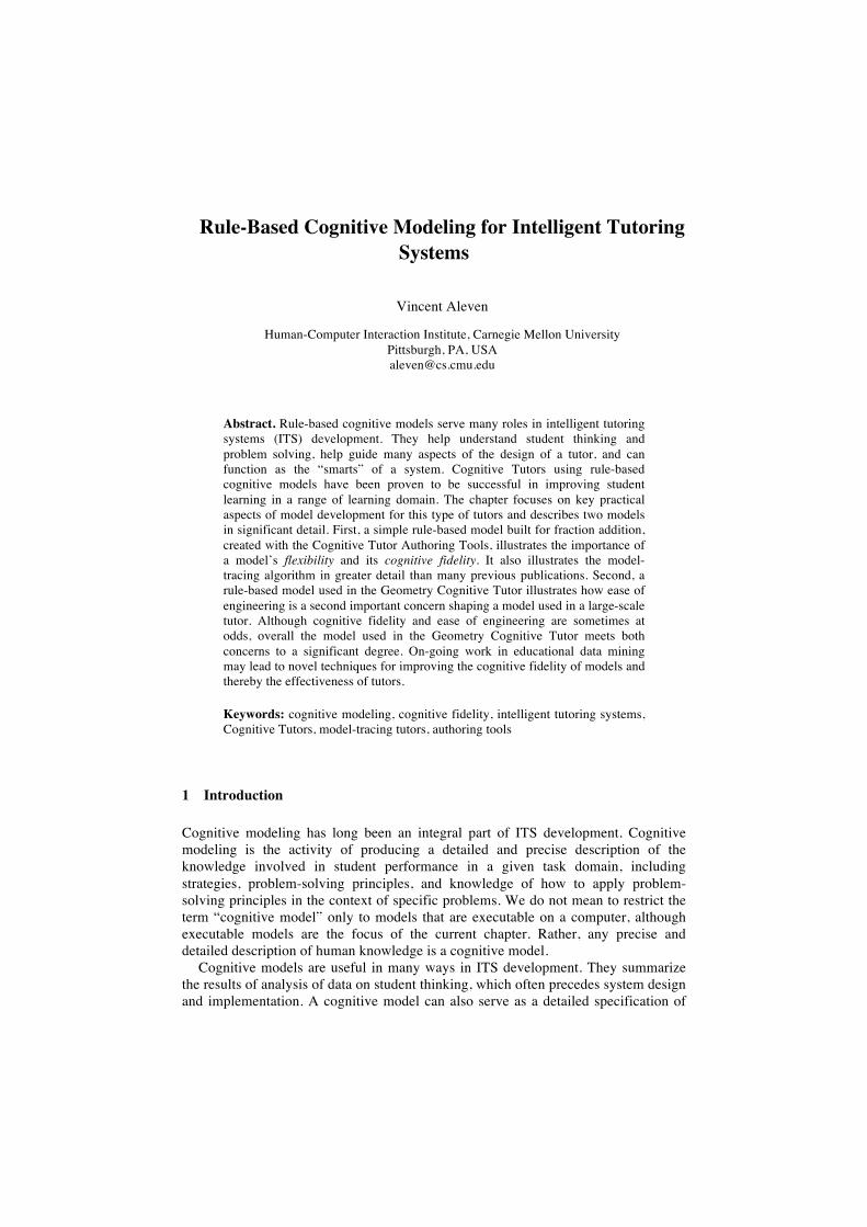
Rule-Based Cognitive Modeling for Intelligent Tutoring Systems

Vincent Aleven

Human-Computer Interaction Institute, Carnegie Mellon University Pittsburgh, PA, USA aleven@cs.cmu.edu

Abstract. Rule-based cognitive models serve many roles in intelligent tutoring systems (ITS) development. They help understand student thinking and problem solving, help guide many aspects of the design of a tutor, and can function as the “smarts” of a system. Cognitive Tutors using rule-based cognitive models have been proven to be successful in improving student learning in a range of learning domain. The chapter focuses on key practical aspects of model development for this type of tutors and describes two models in significant detail. First, a simple rule-based model built for fraction addition, created with the Cognitive Tutor Authoring Tools, illustrates the importance of a model’s flexibility and its cognitive fidelity. It also illustrates the model-tracing algorithm in greater detail than many previous publications. Second, a rule-based model used in the Geometry Cognitive Tutor illustrates how ease of engineering is a second important concern shaping a model used in a large-scale tutor. Although cognitive fidelity and ease of engineering are sometimes at odds, overall the model used in the Geometry Cognitive Tutor meets both concerns to a significant degree. On-going work in educational data mining may lead to novel techniques for improving the cognitive fidelity of models and thereby the effectiveness of tutors.

Keywords: cognitive modeling, cognitive fidelity, intelligent tutoring systems, Cognitive Tutors, model-tracing tutors, authoring tools

1 Introduction

Cognitive modeling has long been an integral part of ITS development. Cognitive modeling is the activity of producing a detailed and precise description of the knowledge involved in student performance in a given task domain, including strategies, problem-solving principles, and knowledge of how to apply problem-solving principles in the context of specific problems. We do not mean to restrict the term “cognitive model” only to models that are executable on a computer, although executable models are the focus of the current chapter. Rather, any precise and detailed description of human knowledge is a cognitive model.

Cognitive models are useful in many ways in ITS development. They summarize the results of analysis of data on student thinking, which often precedes system design and implementation. A cognitive model can also serve as a detailed specification of

the competencies (or skills) targeted by an ITS, and as such, can guide many aspects of the design of the ITS. A deep and detailed understanding of the competencies being targeted in any instructional design effort is likely to lead to better instruction [18]. Further, when a cognitive model is implemented in a language that is executable on a computer, it can function as the “smarts” of the ITS driving the tutoring.

Two types of cognitive models used frequently in ITS are rule-based models [8] [22] [25][44] and constraint-based models [34]. Whereas rule-based models capture the knowledge involved in generating solutions step-by-step, constraint-based models express the requirements that all solutions should satisfy. Both types of models have been used in successful real-world ITS. For each type of model, mature and efficient authoring tools exist [2][35]. The current chapter focuses on the models used in Cognitive Tutors, a widely used type of ITS [8][28][30]. Tutors of this type use a rule-based model, essentially a simulation of student thinking that solves problems in the same way that students are learning to do. The tutor interprets student performance and tracks student learning in terms of the knowledge components defined in the cognitive model. Cognitive Tutors have been shown in many scientific studies to improve student learning in high-school and middle-school mathematics courses, and at the time of this writing, are being used in the US by about 500,000 students annually.

A key concern when developing cognitive models is the degree to which a model faithfully mimics details of human thinking and problem solving. Cognitive scientists have long used rule-based models as a tool to study human thinking and problem solving [5][39]. Their models aim to reproduce human thinking and reasoning in significant detail. Often, they take great care to ensure that their models observe properties and constraints of the human cognitive architecture. Outside of basic cognitive science, accurately modeling details of human cognition and problem solving is important in tutor development. We find it helpful to distinguish two main requirements. First, a model used in a tutor must be flexible in the sense that it covers the sometimes wide variety in students’ solution paths within the given task domain, as well as the different order of steps within each path. This kind of flexibility ensures that the tutor can follow along with students as they solve problems, regardless of how they go about solving them. Second, it is important that a model partitions the problem-solving knowledge within the given task domain in accordance with psychological reality. We use the term cognitive fidelity to denote this kind of correspondence with human cognition. As discussed further below, a model with high cognitive fidelity leads to a tutor that has a more accurate student model and is better able to adapt its instruction to individual students. To achieve flexibility and cognitive fidelity, it helps to perform cognitive task analysis as an integral part of model development. This term denotes a broad array of methods and techniques that cognitive scientists use to understand the knowledge, skills, and strategies involved in skilled performance in a given task domain, as well as the preconceptions, prior knowledge, and the sometimes surprising strategies with which novices approach a task [32]. Although cognitive task analysis and cognitive modeling tend to be (and should be) closely intertwined in ITS development [11], the current chapter focuses on cognitive modeling only.

A third main concern in the development of cognitive models is ease of engineering. ITS have long been difficult to build. It has been estimated, based on the

experience in real-world projects, that it takes about 200-300 hours of highly-skilled labor to produce one hour of instruction with an ITS [36][45]. Some approaches to building ITS, such as example-tracing tutors [1][3] and constraint-based tutors [34], improve upon these development times. Rule-based systems, too, have become easier to build due to improved authoring tools [2] and remain a popular option [20][41]. Nonetheless, building tutors remains a significant undertaking. In creating tutors with rule-based cognitive models, a significant amount of development time is devoted to creating the model itself. It may come as no surprise that ITS developers carefully engineer models so as to reduce development time. Further, being real-world software systems, ITS must heed such software engineering considerations as modularity, ease of maintenance, and scalability. Thus, the models built for real-world ITS reflect engineering concerns, not just flexibility and cognitive fidelity. Sometimes, these aspects can go hand in hand, but at other times, they conflict and must be traded off against each other, especially when creating large-scale systems.

We start with a brief description of Cognitive Tutors and the way they use rule-based models to provide tutoring. We describe two examples of cognitive models used in Cognitive Tutors. The first example describes a model for a relatively simple cognitive skill, fraction addition, and emphasizes flexibility and cognitive fidelity. The second example illustrates how the cognitive model of a real-world tutor, the Geometry Cognitive Tutor, is (arguably) a happy marriage between flexibility, cognitive fidelity, and ease of engineering. Although we have tried to make the chapter self-contained, some knowledge of ITS and some knowledge of production rule systems or rule-based programming languages is helpful. Although many excellent descriptions of model tracing and Cognitive Tutors exist [5][8][25][28][30][40], the current chapter focuses in greater detail than many previous articles on the requirements and pragmatics of authoring a model for use in a Cognitive Tutor.

2 Cognitive Tutors

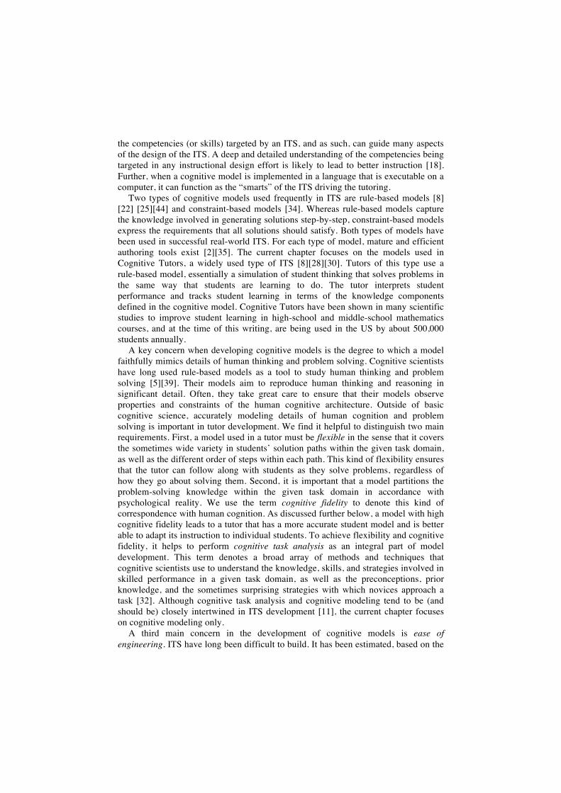
Before describing examples of rule-based models used in ITS, we briefly describe Cognitive Tutors [30]. Like many ITS, Cognitive Tutors provide step-by-step guidance as a student learns a complex problem-solving skill through practice [43]. They typically provide the following forms of support: (a) a rich problem-solving environment that is designed to make “thinking visible,” for example, by prompting for intermediate reasoning steps, (b) feedback on the correctness of these steps, not just the final solution to a problem; often, multiple solution approaches are possible, (c) error-specific feedback messages triggered by commonly occurring errors, (d) context-sensitive next-step hints, usually made available at the student’s request, and (e) individualized problem selection, based on a detailed assessment of each individual student’s problem-solving skill (“cognitive mastery learning” [21]). A Cognitive Tutor for geometry problem solving is shown in Figure 1. This tutor, a precursor of which was developed in our lab, is part of a full-year geometry course, in which students work with the tutor about 40% of the classroom time.

Figure 1: A Cognitive Tutor for geometry problem solving

A number of studies have shown that curricula involving Cognitive Tutors lead to

greater learning by students than the standard commercial math curricula used as comparison curricula [25][28]. Cognitive Tutors also have been successful commercially. A Pittsburgh-based company called Carnegie Learning, Inc., sells middle-school and high-school mathematics curricula of which Cognitive Tutors are integrated parts. At the time of this writing, about 500,000 students in the US use Cognitive Tutors as part of their regular mathematics instruction.

Cognitive Tutors are grounded in ACT-R, a comprehensive theory of cognition and learning [5][9]. A key tenet of this theory is that procedural knowledge, the kind of knowledge that is exercised in skilled task performance, is strengthened primarily through practice. ACT-R stipulates further that production rules are a convenient formalism for describing the basic components of procedural knowledge. Each production rule associates particular actions with the conditions under which these actions are appropriate. The actions can be mental actions (e.g., a calculation in the head, or a decision which part of the problem to focus on next) or physical actions (e.g., writing down an intermediate step in problem solving). Production rules are commonly written in IF-THEN format, with the “THEN part” or “right-hand side” describing actions and the “IF-part” or “left-hand side” describing conditions under which these actions are appropriate.

Reflecting the roots of this technology in the ACT-R theory, each Cognitive Tutor has a rule-based cognitive model as its central component. The models used in Cognitive Tutors are simulations of student thinking that can solve problems in the multiple ways that students can (or are learning to). The models can also be viewed as detailed specifications of the skills targeted in the instruction with the tutor. Cognitive

Tutors use their cognitive models to provide tutoring by means of an algorithm called model tracing [8]. The tutor assesses and interprets students’ solution steps by comparing what the student does in any given situation against what the model might do in the same situation. The basic idea is straightforward: After each student attempt at solving a step in a tutor problem, the tutor runs its model to generate all possible next actions that the model can produce. The student action is deemed correct only if it is among the multiple actions that the model can take next. If the student action is not among the potential next steps, it is deemed incorrect. When a student action is deemed correct, the production rules that generate the matching action serve as an interpretation of the thinking process by which the student arrived at this step. This detailed information enables the system to track, over time, how well an individual student masters these skills. A popular method for doing so is a Bayesian algorithm called knowledge tracing [19][21], which provides an estimate of the probability that the student masters each targeted skill. Some cognitive models contain rules that are represent incorrect behavior, enabling the tutor, through the same model-tracing process, to recognize commonly occurring errors and provide error-specific feedback.

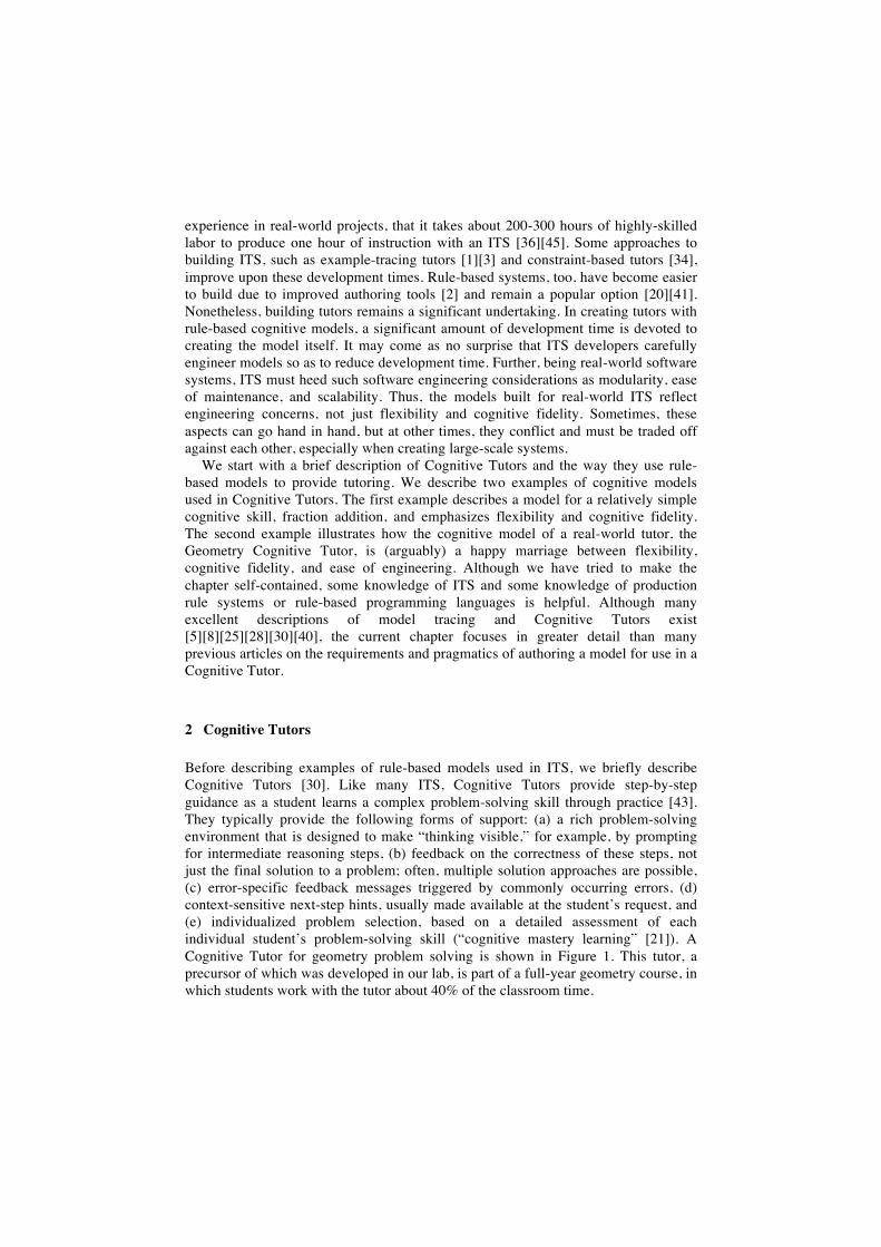
Figure 2: Demo tutor for fraction addition being built with CTAT

3 A simple example of a cognitive model

Our first example is a simple rule-based cognitive model for fraction addition. This example emphasizes flexibility and cognitive fidelity; engineering concerns are in the background with a small model such as this. We also illustrate the model-tracing algorithm in the current section. The fraction addition model is not in use in a real-world tutor, although it is a realistic model for the targeted skill. The model is part of a demo tutor that comes with the Cognitive Tutor Authoring Tools (CTAT)[2][3]; see Figure 2 for a view of this tutor as it is being authored with CTAT. These tools

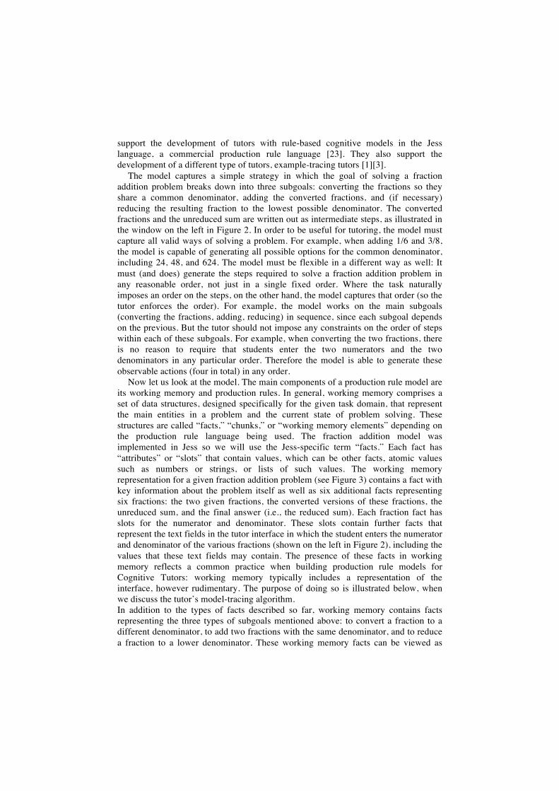
support the development of tutors with rule-based cognitive models in the Jess language, a commercial production rule language [23]. They also support the development of a different type of tutors, example-tracing tutors [1][3].

The model captures a simple strategy in which the goal of solving a fraction addition problem breaks down into three subgoals: converting the fractions so they share a common denominator, adding the converted fractions, and (if necessary) reducing the resulting fraction to the lowest possible denominator. The converted fractions and the unreduced sum are written out as intermediate steps, as illustrated in the window on the left in Figure 2. In order to be useful for tutoring, the model must capture all valid ways of solving a problem. For example, when adding 1/6 and 3/8, the model is capable of generating all possible options for the common denominator, including 24, 48, and 624. The model must be flexible in a different way as well: It must (and does) generate the steps required to solve a fraction addition problem in any reasonable order, not just in a single fixed order. Where the task naturally imposes an order on the steps, on the other hand, the model captures that order (so the tutor enforces the order). For example, the model works on the main subgoals (converting the fractions, adding, reducing) in sequence, since each subgoal depends on the previous. But the tutor should not impose any constraints on the order of steps within each of these subgoals. For example, when converting the two fractions, there is no reason to require that students enter the two numerators and the two denominators in any particular order. Therefore the model is able to generate these observable actions (four in total) in any order.

Now let us look at the model. The main components of a production rule model are its working memory and production rules. In general, working memory comprises a set of data structures, designed specifically for the given task domain, that represent the main entities in a problem and the current state of problem solving. These structures are called “facts,” “chunks,” or “working memory elements” depending on the production rule language being used. The fraction addition model was implemented in Jess so we will use the Jess-specific term “facts.” Each fact has “attributes” or “slots” that contain values, which can be other facts, atomic values such as numbers or strings, or lists of such values. The working memory representation for a given fraction addition problem (see Figure 3) contains a fact with key information about the problem itself as well as six additional facts representing six fractions: the two given fractions, the converted versions of these fractions, the unreduced sum, and the final answer (i.e., the reduced sum). Each fraction fact has slots for the numerator and denominator. These slots contain further facts that represent the text fields in the tutor interface in which the student enters the numerator and denominator of the various fractions (shown on the left in Figure 2), including the values that these text fields may contain. The presence of these facts in working memory reflects a common practice when building production rule models for Cognitive Tutors: working memory typically includes a representation of the interface, however rudimentary. The purpose of doing so is illustrated below, when we discuss the tutor’s model-tracing algorithm. In addition to the types of facts described so far, working memory contains facts representing the three types of subgoals mentioned above: to convert a fraction to a different denominator, to add two fractions with the same denominator, and to reduce a fraction to a lower denominator. These working memory facts can be viewed as

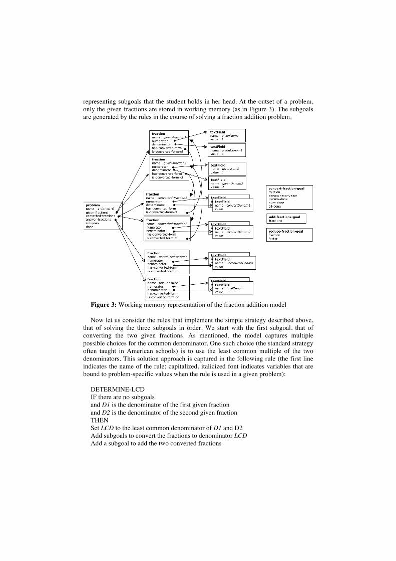
representing subgoals that the student holds in her head. At the outset of a problem, only the given fractions are stored in working memory (as in Figure 3). The subgoals are generated by the rules in the course of solving a fraction addition problem.

Figure 3: Working memory representation of the fraction addition model Now let us consider the rules that implement the simple strategy described above,

that of solving the three subgoals in order. We start with the first subgoal, that of converting the two given fractions. As mentioned, the model captures multiple possible choices for the common denominator. One such choice (the standard strategy often taught in American schools) is to use the least common multiple of the two denominators. This solution approach is captured in the following rule (the first line indicates the name of the rule; capitalized, italicized font indicates variables that are bound to problem-specific values when the rule is used in a given problem):

DETERMINE-LCD IF there are no subgoals and D1 is the denominator of the first given fraction and D2 is the denominator of the second given fraction THEN Set LCD to the least common denominator of D1 and D2 Add subgoals to convert the fractions to denominator LCD Add a subgoal to add the two converted fractions

Due to space limitations, we do not present the Jess versions of these rules. The interested reader could download CTAT from http://ctat.pact.cs.cm.edu, install it, and explore the demo model. The DETERMINE-LCD rule models a first thinking step in solving a fraction addition problem. The conditions of this rule, that there are two given fractions and no subgoals, are met at the beginning of each problem. On its right-hand side, the rule sets a number of subgoals, meaning that it creates facts in working memory that represent these subgoals. In this way, the model models unobservable mental actions, namely, a student’s planning, in their head, of the things they need to do in order to solve the problem. The DETERMINE-LCD rule does not actually model how to determine the least common multiple of two numbers – instead it uses a function call on the right-hand side of the rule. It is assumed that the student has learned how to determine the least common denominator prior to learning fraction addition, and therefore detailed modeling of that skill is not necessary.

In addition to the DETERMINE-LCD rule, the model contains three rules that capture alternative solution approaches and one rule that captures a common error. A rule named DETERMINE-PRODUCT uses the product of the two denominators as the common denominator, rather than their least common multiple, but is otherwise the same as DETERMINE-LCD. A second rule named DETERMINE-COMMON-MULTIPLE uses any common multiple. Although this rule is the same “in spirit” as the previous two, its implementation is different, due to the fact that it must generate any value that is a common multiple of the denominators. Rather than generate a random value for the common denominator (which would almost never be the value that the student actually used, meaning that such a rule would be useless for model tracing), the rule always “happens” to use the value that the student is actually using, provided it is a common multiple of the two denominators. One might say the rule guesses right as to what the student is doing. (It is able to do so because the actual student value is made available to the model by the tutor architecture. The demo model that comes with CTAT (version 2.9 and later) provides further detail.) Third, when the denominators of the two fractions are the same, no conversion is necessary. A rule called SAME-DENOMINATORS applies in this particular situation. Finally, the model captures a rule that models the common error of adding the denominators rather than computing a common multiple. This rule, called BUG-DETERMINE-SUM, is the same as DETERMINE-LCD and DETERMINE-PRODUCT, except that it sets the common denominator to the sum of the two denominators. This rule is marked as representing incorrect behavior, simply by including the word “BUG” in the name of the rule. The model contains two more rules corresponding to the subgoal to convert the fractions. These rules take care of converting the numerator and of writing out the converted fractions, once a common denominator has been determined.

CONVERT-DENOMINATOR IF there is a subgoal to convert fraction F so that the denominator is D And the denominator for the converted fraction has not been entered yet THEN Write D as the denominator of the converted fraction And make a note that the denominator has been taken care of

CONVERT-NUMERATOR IF there is a subgoal to convert fraction F so that the denominator is D And the numerator for the converted fraction has not been entered yet And the (original) numerator of F is NUM And the (original) denominator of F is DENOM THEN Write NUM * (D / DENOM) as the numerator of the converted fraction And make a note that the numerator has been taken care of The conditions of these two rules require that a common denominator has been

determined and a “convert-fraction” subgoal has been created. That is, these rules are not activated (i.e., do not match working memory) until one of the “DETERMINE-…” rules described above has been executed. On their right-hand-side, the rules model physical actions (“Write …”), namely, the action of entering the value for the denominator or numerator into the relevant text field in the tutor interface. These actions are modeled as modifications of facts in working memory that correspond to the relevant interface component, although that fact is hard to glean this from the pseudo code. The reader may want to look at the actual Jess code. In addition to the rules described so far, the model contains a number of other rules related to the other main subgoals, but we do not have the space to describe them.

Let us now look at how the model-tracing algorithm uses the model to provide tutoring [8][10]. This algorithm is specific to ITS; it is not used in standard production rule systems. As discussed below, model tracing is somewhat similar to, but also very different from, the standard conflict-resolution method used in production rule systems. Simply put, model tracing is the process of figuring out, for any given student action in the tutor interface, what sequence of rule activations (if any) produces the same action. Therefore, just as standard conflict resolution, model tracing is about choosing from among possible rule activations. (A “rule activation” is the combination of a production rule and a set of bindings for its variables. Rule activations are created when a rule is matched against working memory. Different production rule languages use different terminology for this notion. “Rule activation” is a Jess term.) For example, at the outset of our example problem 1/6 + 3/8, a student might, as her first action, enter “24” as the denominator of the second converted fraction. (Note that this denominator is the least common multiple of the two denominators 6 and 8.) The fraction addition model can generate this action, starting with the initial working memory representation, by executing an activation of rule DETERMINE-LCD followed by one of CONVERT-DENOMINATOR, both described above. As an alternative first action, an (adventurous) student might enter “624” as the numerator of the first converted fraction. The model can also generate this action, namely, by executing activations of DETERMINE-COMMON-MULTIPLE and CONVERT-NUMERATOR. Third, a students might (erroneously) enter “14” as the numerator of one of the converted fractions. The model can generate this action by executing activations of BUG-DETERMINE-SUM and CONVERT-DENOMINATOR. Finally, a fourth student might enter “9” as the denominator of the first converted fraction. The model cannot generate this action. No sequence of rule activations produces this action.

As mentioned, the purpose of model tracing is to assess student actions and to interpret them in terms of underlying knowledge components. The first two of our example actions can be “modeled” by rules in the model that represent correct behavior. Therefore, they are deemed correct by the model tracer (and tutor). The production rules that generate the observable action provide an interpretation of the student action in terms of underlying skills. Interestingly, the different actions are modeled by different rules; in other words, they are interpreted as involving different skills. The third student action is modeled also, but one of the rules that is involved represents incorrect behavior. This action is therefore considered to be incorrect. The tutor displays an error message associated with the rule. (“It looks like you are adding the denominators, but you need a common multiple.”) Since the model cannot generate the fourth action, the tutor will mark it to be incorrect.

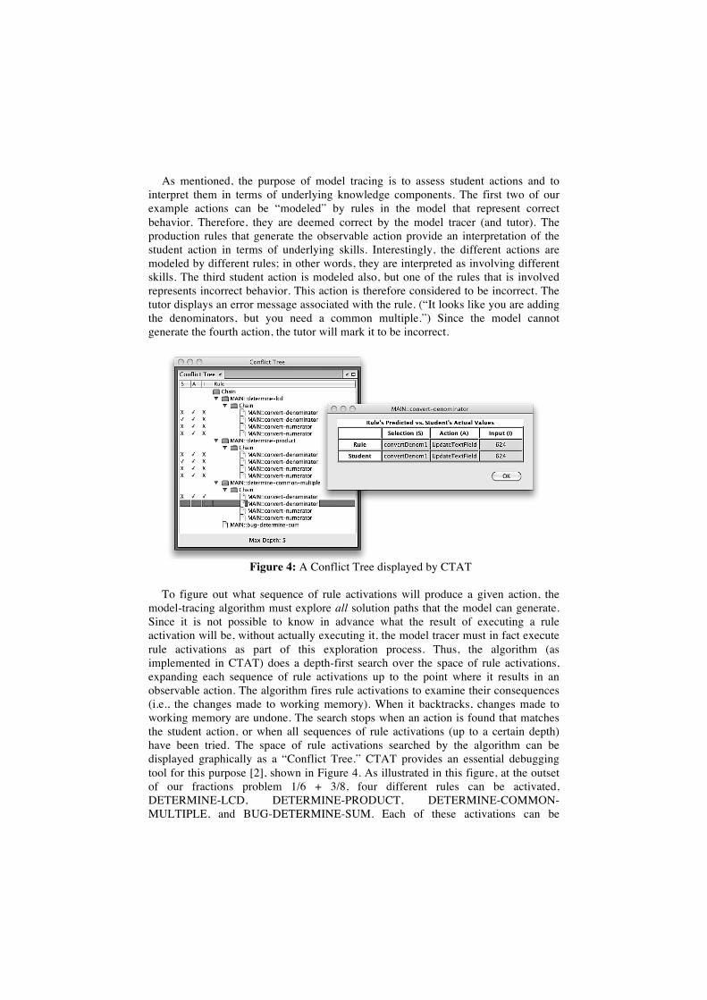
Figure 4: A Conflict Tree displayed by CTAT

To figure out what sequence of rule activations will produce a given action, the

model-tracing algorithm must explore all solution paths that the model can generate. Since it is not possible to know in advance what the result of executing a rule activation will be, without actually executing it, the model tracer must in fact execute rule activations as part of this exploration process. Thus, the algorithm (as implemented in CTAT) does a depth-first search over the space of rule activations, expanding each sequence of rule activations up to the point where it results in an observable action. The algorithm fires rule activations to examine their consequences (i.e., the changes made to working memory). When it backtracks, changes made to working memory are undone. The search stops when an action is found that matches the student action, or when all sequences of rule activations (up to a certain depth) have been tried. The space of rule activations searched by the algorithm can be displayed graphically as a “Conflict Tree.” CTAT provides an essential debugging tool for this purpose [2], shown in Figure 4. As illustrated in this figure, at the outset of our fractions problem 1/6 + 3/8, four different rules can be activated, DETERMINE-LCD, DETERMINE-PRODUCT, DETERMINE-COMMON-MULTIPLE, and BUG-DETERMINE-SUM. Each of these activations can be

followed by four different rule activations, two each for CONVERT-DENOMINATOR and CONVERT-NUMERATOR. (The Conflict Tree does not contain activations of these rules following BUG-DETERMINE-SUM, because the search stops before that part of the search space is reached.) Appropriately, the Conflict Tree does not show any activations of the SAME-DENOMINATORS rule; this rule’s condition, that the two denominators are the same, is not met.

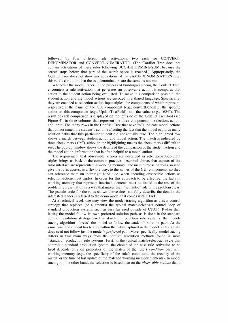
Whenever the model tracer, in the process of building/exploring the Conflict Tree, encounters a rule activation that generates an observable action, it compares that action to the student action being evaluated. To make this comparison possible, the student action and the model actions are encoded in a shared language. Specifically, they are encoded as selection-action-input triples, the components of which represent, respectively, the name of the GUI component (e.g., convertDenom1), the specific action on this component (e.g., UpdateTextField), and the value (e.g., “624”). The result of each comparison is displayed on the left side of the Conflict Tree tool (see Figure 4), in three columns that represent the three components – selection, action, and input. The many rows in the Conflict Tree that have “×”s indicate model actions that do not match the student’s action, reflecting the fact that the model captures many solution paths that this particular student did not actually take. The highlighted row shows a match between student action and model action. The match is indicated by three check marks (“√”), although the highlighting makes the check marks difficult to see. The pop-up window shows the details of the comparison of the student action and the model action, information that is often helpful to a model author.

The requirement that observable actions are described as selection-action-input triples brings us back to the common practice, described above, that aspects of the tutor interface are represented in working memory. The main purpose of doing so is to give the rules access, in a flexible way, to the names of the GUI components, so they can reference them on their right-hand side, when encoding observable actions as selection-action-input triples. In order for this approach to be effective, the facts in working memory that represent interface elements must be linked to the rest of the problem representation in a way that makes their “semantic” role in the problem clear. The pseudo code for the rules shown above does not fully describe the details; the interested reader is referred to the demo model that comes with CTAT.

At a technical level, one may view the model-tracing algorithm as a new control strategy that replaces (or augments) the typical match-select-act control loop of standard production systems such as Jess (as used outside of CTAT). Rather than letting the model follow its own preferred solution path, as is done in the standard conflict resolution strategy used in standard production rule systems, the model-tracing algorithm “forces” the model to follow the student’s solution path. At the same time, the student has to stay within the paths captured in the model, although she does need not follow just the model’s preferred path. More specifically, model tracing differs in two main ways from the conflict resolution methods found in most “standard” production rule systems. First, in the typical match-select-act cycle that controls a standard production system, the choice of the next rule activation to be fired depends only on properties of the match of the rule’s condition part with working memory (e.g., the specificity of the rule’s conditions, the recency of the match, or the time of last update of the matched working memory elements). In model tracing, on the other hand, the selection is based also on the observable actions that a

rule activation generates (as part of its action part). A second difference is that the model tracer, as it searches for actions the model might generate, searches for (and selects for execution) sequences of multiple rule activations, rather than just for single rule activations. Put differently, standard production systems do conflict resolution over (a set of) single rule activations, whereas the model-tracing algorithm does conflict resolution over (a set of) chains of rule activations.

Returning to one of our main themes, let us review how the requirements of flexibility and cognitive fidelity have helped shape the fraction addition model. First, consider the ways in which the model is flexible – it generates solutions with different common denominators and with different step order. That is, it faithfully mimics the expected variability of students’ problem-solving processes in terms of observable actions. This flexibility is motivated by pedagogical considerations. It is necessary if the tutor is to respond (with positive feedback) to all students’ reasonable solution approaches and not to impose arbitrary restrictions on student problem solving that make the student’s learning task harder than necessary.

Second, the model arguably has strong cognitive fidelity. Key strategies such as using the least common multiple of the two given denominators, the product of the two denominators, or any other common multiple of the two denominators are modeled by separate rules, even though they could have been modeled more easily by a single rule. By modeling them as separate rules, the model reflects the conjecture that they represent different skills that a student learns separately, as opposed to being different surface manifestations of the same underlying student knowledge (e.g., special cases of a single unified strategy). These two possibilities lead to markedly different predictions about learning and transfer. If skills are learned separately, then practice with one does not have an effect on the other. On the other hand, if seemingly different skills reflect a common strategy, then practice with one should lead to better performance on the other. Since we do not know of a “grand unified denominator strategy” that unifies the different approaches, we make the assumption that the different strategies indeed reflect separate cognitive skills that are learned separately. To the extent that this assumption is correct, the current model (with separate skills) can be said to have greater cognitive fidelity than a model that models the strategies with a single rule.1 It partitions the knowledge in a way that reflects the psychological reality of student thinking and learning, and presumably leads to accurate transfer predictions.

Incidentally, the model does not contain a separate rule for the situation where one denominator is a multiple of the other. In this situation, the larger of the two denominators could serve as the common denominator, and there is no need to compute the product or to try to compute the least common denominator. It is quite possible that this strategy is learned separately as well. If so, then a model that modeled this strategy with a separate rule would have greater cognitive fidelity than the current model.

1 Ideally, the assumptions being made about how students solve fraction addition problems

would be backed up by data about student thinking gathered through cognitive task analysis, or by results of mining student-tutor interaction data. We return to this point in the final section of the chapter.

Why does such detailed attention to cognitive fidelity matter? Cognitive fidelity helps in making sure that a student’s successes and errors in problem solving are attributed to the appropriate skills or are blamed on the appropriate lack of skills. In turn, appropriate attribution of successes and errors helps the tutor maintain an accurate student model through knowledge tracing. In turn, a more accurate student model may lead to better task selection decisions by the tutor, since (in Cognitive Tutors and many other ITS), these decisions are informed by the student model [21]. Therefore, greater cognitive fidelity may result in more effective and/or more efficient student learning. So far, this prediction has not been tested empirically, although this very question is an active area of research. We return to this point in the final section of the chapter.

4 Cognitive modeling for a real-world tutor: The Geometry Cognitive Tutor

In this section, we present a case study of cognitive modeling for a real-world intelligent tutoring system, namely, the model of the first version of the Geometry Cognitive Tutor described above, developed in our lab in the mid and late 1990s. This tutor is part of a full-year geometry curriculum, which has been shown to improve student learning, relative to a comparison curriculum [31]. The current Geometry Cognitive Tutor, which derives from the one described in this section, is in use in approximately 1,000 schools in the US (as of May 2010). The case study illustrates that flexibility and cognitive fidelity, emphasized in the fraction addition example, are not the only concerns when creating a model for a large real-world tutor. In a larger effort such as the Geometry Cognitive Tutor, engineering concerns inevitably come to the forefront, due to resource limitations. Arguably, the model for the Geometry Cognitive Tutor represents a happy marriage between flexibility, cognitive fidelity, and engineering. Although the description in this chapter ignores many details of the model, it highlights the model’s essential structure and the major design decisions that helped shape it.

The model we describe is the third in a line of cognitive models for geometry developed for use in Cognitive Tutors. The first one was a model for geometry proof, developed by John Anderson and colleagues, and used in the original Geometry Proof Tutor which in lab studies was shown to be highly effective in improving student learning [5][6][7]. The second was developed by Ken Koedinger and captures the knowledge structures that enable experts to plan and generate proof outlines without doing the extensive search that characterizes novices’ proof-generation efforts [26][27]. The third model in this line (and the one on which we focus in the current chapter) was developed and then re-implemented by Ken Koedinger and colleagues, including the chapter author [4]. Unlike the fraction addition model, which was implemented using the CTAT authoring tools in the Jess production rule language, the geometry model was implemented in the Tertle production rule language, which was created in our lab and is geared specifically towards model tracing [10]. We focus on the Angles unit, one of six units that (at the time) made up the tutor’s curriculum. This unit deals with the geometric properties of angles and covers 17 theorems. Other units dealt with Area, the Pythagorean Theorem, Similar Triangles, Quadrilaterals, and

Circles. Units dealing with Right Triangle Trigonometry, Transformations, and 3D Geometry were added later. The curriculum was re-structured later, and the current tutor has 41 units. The model described here was used in the Angles, Circles, and Quadrilaterals units, and comprises approximately 665 rules. As mentioned, this model covers only part of the tutor’s curriculum.

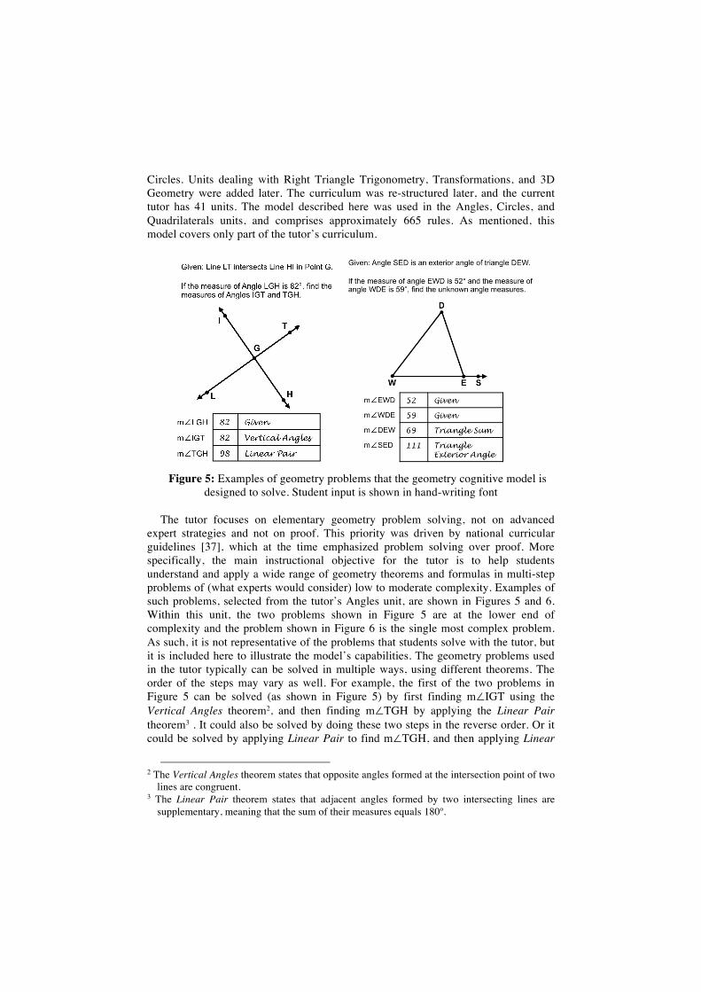
Figure 5: Examples of geometry problems that the geometry cognitive model is

designed to solve. Student input is shown in hand-writing font

The tutor focuses on elementary geometry problem solving, not on advanced expert strategies and not on proof. This priority was driven by national curricular guidelines [37], which at the time emphasized problem solving over proof. More specifically, the main instructional objective for the tutor is to help students understand and apply a wide range of geometry theorems and formulas in multi-step problems of (what experts would consider) low to moderate complexity. Examples of such problems, selected from the tutor’s Angles unit, are shown in Figures 5 and 6. Within this unit, the two problems shown in Figure 5 are at the lower end of complexity and the problem shown in Figure 6 is the single most complex problem. As such, it is not representative of the problems that students solve with the tutor, but it is included here to illustrate the model’s capabilities. The geometry problems used in the tutor typically can be solved in multiple ways, using different theorems. The order of the steps may vary as well. For example, the first of the two problems in Figure 5 can be solved (as shown in Figure 5) by first finding m∠IGT using the Vertical Angles theorem2, and then finding m∠TGH by applying the Linear Pair theorem3 . It could also be solved by doing these two steps in the reverse order. Or it could be solved by applying Linear Pair to find m∠TGH, and then applying Linear

2 The Vertical Angles theorem states that opposite angles formed at the intersection point of two

lines are congruent. 3 The Linear Pair theorem states that adjacent angles formed by two intersecting lines are

supplementary, meaning that the sum of their measures equals 180º.

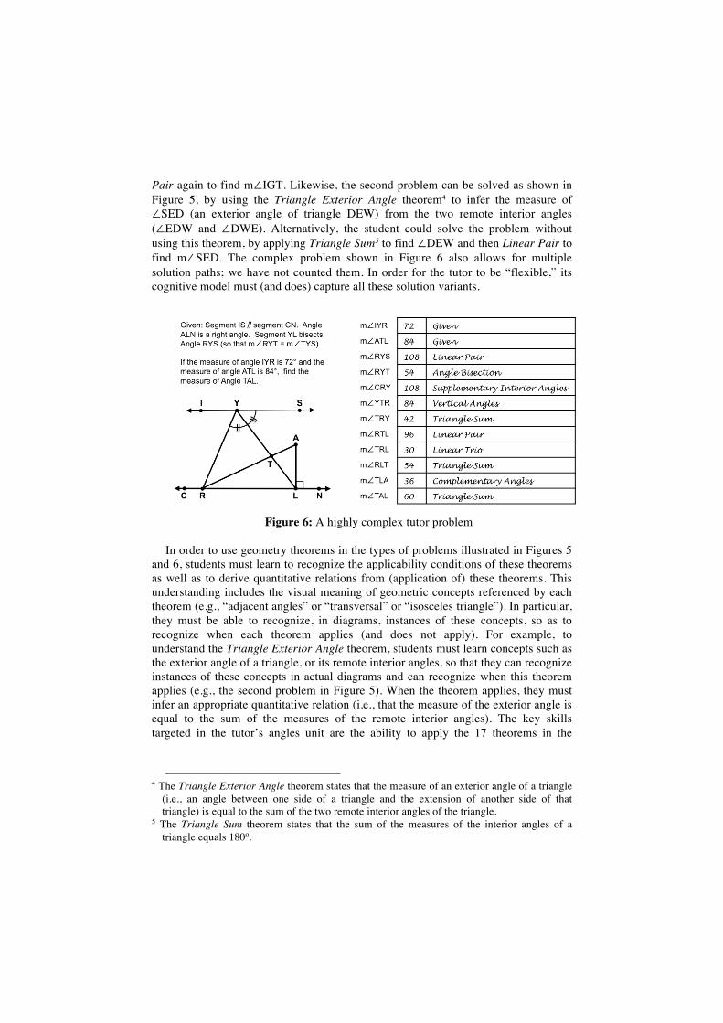
Pair again to find m∠IGT. Likewise, the second problem can be solved as shown in Figure 5, by using the Triangle Exterior Angle theorem4 to infer the measure of ∠SED (an exterior angle of triangle DEW) from the two remote interior angles (∠EDW and ∠DWE). Alternatively, the student could solve the problem without using this theorem, by applying Triangle Sum5 to find ∠DEW and then Linear Pair to find m∠SED. The complex problem shown in Figure 6 also allows for multiple solution paths; we have not counted them. In order for the tutor to be “flexible,” its cognitive model must (and does) capture all these solution variants.

Figure 6: A highly complex tutor problem

In order to use geometry theorems in the types of problems illustrated in Figures 5

and 6, students must learn to recognize the applicability conditions of these theorems as well as to derive quantitative relations from (application of) these theorems. This understanding includes the visual meaning of geometric concepts referenced by each theorem (e.g., “adjacent angles” or “transversal” or “isosceles triangle”). In particular, they must be able to recognize, in diagrams, instances of these concepts, so as to recognize when each theorem applies (and does not apply). For example, to understand the Triangle Exterior Angle theorem, students must learn concepts such as the exterior angle of a triangle, or its remote interior angles, so that they can recognize instances of these concepts in actual diagrams and can recognize when this theorem applies (e.g., the second problem in Figure 5). When the theorem applies, they must infer an appropriate quantitative relation (i.e., that the measure of the exterior angle is equal to the sum of the measures of the remote interior angles). The key skills targeted in the tutor’s angles unit are the ability to apply the 17 theorems in the

4 The Triangle Exterior Angle theorem states that the measure of an exterior angle of a triangle

(i.e., an angle between one side of a triangle and the extension of another side of that triangle) is equal to the sum of the two remote interior angles of the triangle.

5 The Triangle Sum theorem states that the sum of the measures of the interior angles of a triangle equals 180º.

manner just described. That is, the tutor interprets student performance and tracks student learning largely at the level of applying individual theorems.

It was decided early on during the design process that the tutor interface would prompt the student for each step in the process of solving a geometry problem, as can be seen in Figures 1 (which is a later version of the same tutor), 5, and 6. That is, for each problem in the tutor, an empty table is given at the outset, with the labels for the angle measures visible. The student completes the problem by filling out in the table, for each step, a value (typically, the measure of an angle) and a justification for the value by citing the name of a theorem. (The value of having students provide justifications for their steps was confirmed by subsequent research [4].) Typically, the steps need not be done strictly in the order in which they appear in the table. Rather, the step order must observe the logical dependencies among the steps, meaning that any given step can be completed only when the logically-prior steps have been completed. Typically, the order of the quantities in the table observes the logical dependencies (and so going in the order of the table usually works), but other orders may be possible as well. The purpose of listing the steps in advance, rather than letting the student figure out what the steps are was to minimize the cognitive load associated with searching for solution paths in diagrams. This kind of search (and the concomitant cognitive load) was thought to hinder the acquisition of problem-solving knowledge. This design was loosely inspired by work by Sweller, van Merriënboer, and Paas [42], who showed that completion problems and goal-free problems lead to superior learning during the early stages of skill acquisition, compared to problem solving. Prompting for steps significantly reduces the need for students to search the diagram in the process of solving a problem. Although experts are adept at searching a diagram in a strategic manner, it was thought that strategic diagram need not be in the foreground in the Geometry Cognitive Tutor. The kinds of highly complex problems in which sophisticated search strategies would pay off were deemed to outside of the scope of the instruction.

These key design decisions had a significant impact on the cognitive model. The model captures a problem-solving approach in which the student, in order to generate a problem-solving action (i.e., the next step in a given problem), takes the following four mental steps:

1. Focus on the next quantity to solve (e.g., by looking at the table). For example, consider a student who works on the first problem in Figure 5, at the point after she has filled out the first row the table (m∠LGH equals 82º as given in the problem statement). Looking at the table, the student might decide to focus on m∠TGH as the next quantity to solve; let us call this quantity the “desired quantity.” (Note that this quantity is listed in the third row of the table. The student skips one of the quantities in the table.)

2. Identify a quantitative relation between the desired quantity and other quantities in the problem, justified by a geometry theorem. Find a way of deriving the value of the desired quantity. For example, searching the diagram, our student might recognize that ∠LGH and ∠TGH form a linear pair and she might derive, by application of the Linear Pair theorem, the quantitative relation m∠LGH + m∠TGH = 180°. Applying her knowledge of arithmetic (or algebra), our student might determine that m∠IGT can be found once m∠LGH is known,

3. Check if a sufficient number of quantities in the selected quantitative relation are known to derive the value of the desired quantity. For example, our student might ascertain (by looking at the table) that the value of m∠LGH (which we call “pre-requisite quantity”) is known.

4. Derive the desired quantity’s value from the quantitative relation using the values of the other known quantities. For example, our student might conclude that m∠ LGH equals 98º and enter this value into the table.

Let us look at the key components of the model in more detail, starting with the organization of working memory. As mentioned, in general, working memory contains a representation of a problem’s structure as well as of its evolving solution state. The geometry model’s working memory contains two main types of elements. (Following the Tertle production rule language, we employ the term “working memory elements” rather than “facts.”) First, working memory lists the key quantities in the given problem, that is, the quantities whose value is given or whose value the student is asked to find. In the tutor unit dealing with angles, the quantities are angle measures. In other units, we encounter arc measures, segment measures, circumference measures, area measures, etc. In addition to the key quantities, working memory contains elements representing quantitative relations among these quantities. These working memory elements specify, for each, the type of quantitative relation, the quantities involved, and the geometry theorem whose application gives rise to (and justifies) the relation. For example, the key quantities in the first problem illustrated in Figure 5 are the measures of the three angles LGH, TGH, and IGT. There are three quantitative relations relating these quantities:

• m∠TGH + m∠IGT = 180°, justified by Linear Pair • m∠LGH + m∠TGH = 180°, justified by Linear Pair • m∠LGH = m∠IGT, justified by Vertical Angles

Similarly, in the second problem, there are four key quantities and three relations, one justified by application of Triangle Sum, one justified by Linear Pair, and one by Triangle Exterior Angle. The third problem involves 12 key quantities and 15 relations between these quantities.

To model quantitative relations in working memory, we created a hierarchy of relation types, a small part of which is shown in Figure 7. This hierarchy reflects both quantitative aspects and geometric aspects of geometry problem solving. It is intended to capture how, over time, geometry problem-solving knowledge might be organized in the student’s mind. At higher levels in this hierarchy, relation types are differentiated based on the number of quantities they involve and on how these quantities are quantitatively related. At the lowest level, subtypes are differentiated on the geometry theorem that justifies the relation. The actual relation instances in working memory are instances of the lowest-level subtypes. For example, quantitative relations that state that two quantities are equal are modeled as “equal-quantities-relation.” The subtypes of this relation differ with respect to the geometry theorem that justifies the relation, such as the Vertical Angles and Alternate Interior Angles theorems. As another example, relations that state that some function of certain quantities (usually, their sum) equals another quantity or a constant are modeled as “N-argument-function.” The (leaf) subtypes of this type are (again) differentiated based on the geometry theorem that gives rise to the relation, such as Triangle Exterior Angle or Linear Pair.

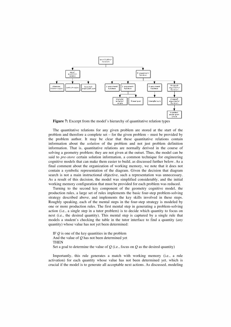
Figure 7: Excerpt from the model’s hierarchy of quantitative relation types The quantitative relations for any given problem are stored at the start of the

problem and therefore a complete set – for the given problem – must be provided by the problem author. It may be clear that these quantitative relations contain information about the solution of the problem and not just problem definition information. That is, quantitative relations are normally derived in the course of solving a geometry problem; they are not given at the outset. Thus, the model can be said to pre-store certain solution information, a common technique for engineering cognitive models that can make them easier to build, as discussed further below. As a final comment about the organization of working memory, we note that it does not contain a symbolic representation of the diagram. Given the decision that diagram search is not a main instructional objective, such a representation was unnecessary. As a result of this decision, the model was simplified considerably, and the initial working memory configuration that must be provided for each problem was reduced.

Turning to the second key component of the geometry cognitive model, the production rules, a large set of rules implements the basic four-step problem-solving strategy described above, and implements the key skills involved in these steps. Roughly speaking, each of the mental steps in the four-step strategy is modeled by one or more production rules. The first mental step in generating a problem-solving action (i.e., a single step in a tutor problem) is to decide which quantity to focus on next (i.e., the desired quantity). This mental step is captured by a single rule that models a student’s checking the table in the tutor interface to find a quantity (any quantity) whose value has not yet been determined:

IF Q is one of the key quantities in the problem And the value of Q has not been determined yet THEN Set a goal to determine the value of Q (i.e., focus on Q as the desired quantity) Importantly, this rule generates a match with working memory (i.e., a rule

activation) for each quantity whose value has not been determined yet, which is crucial if the model is to generate all acceptable next actions. As discussed, modeling

all solution paths is a major precondition for models used for tutoring (by model tracing). Although in this first mental step, any key quantity whose value has not been determined yet can be chosen, the later mental steps impose additional restrictions. That is, not all choices for the desired quantity made in this first step will “survive” the later steps. As a final comment about this rule, there are other possible ways, besides looking at the table, in which a student might decide on the next desired quantity. For example, a student might search the diagram for an angle whose measure can be determined next. Such diagrammatic reasoning is not modeled, however, as discussed above.

The second mental step has two parts, namely, (a) to identify a quantitative relation that can be applied to find the desired quantity, justified by a geometry theorem, and (b) to determine a set of “pre-requisite quantities” from which the value of the desired quantity can be derived. For example, assume that the model is working on the first problem in Figure 5, at a point where it has determined that m∠LGH = 82°. (This value is given in the problem statement.) If in mental step 1, the model selects m∠TGH as the desired quantity, then in mental step 2 (the current step), it may infer that the desired quantity can be derived from the quantitative relation m∠LGH + m∠TGH = 180°, justified by Linear Pair, once m∠LGH and the constant 180° are known (i.e., the latter two quantities are the pre-requisite quantities). Presumably, the student would recognize the applicability of Linear Pair by searching the diagram. The cognitive model does not capture this kind of diagrammatic reasoning, however. Instead, it looks for a quantitative relation in working memory that involves the desired quantity – as mentioned, all quantitative relations for the given problem are pre-stored. Having found a relation from which the desired quantity can be derived, the model determines the pre-requisite quantities through quantitative reasoning. To model this kind of reasoning, the model contains a separate rule (or rules) for each quantitative relation defined at the intermediate levels of the hierarchy. For example, application of Linear Pair (as well as application of Angle Addition, Complementary Angles, etc.) yields a “two-argument function” (e.g., m∠LGH + m∠TGH = 180°). This kind of relation asserts that a function of two quantities, called “input quantities,” is equal to a third quantity or constant, called “output quantity.” The relation may be applied either forwards or backwards. In our running example, the relation must be applied backward to derive the desired quantity:

IF there is a goal to find the value of quantity Q And R is a two-argument-function And Q is one of the input quantities of R And Q1 is the other input quantity of R And Q2 is the output quantity of R THEN Set a goal to apply R backwards with Q1 and Q2 as pre-requisite quantities This rule and the many other rules like it model the quantitative reasoning involved

in geometry problem solving. The use of the hierarchy of quantitative relations is a significant advantage in defining these rules (which was the main reason for creating it in the first place). Because the rules are defined at the intermediate levels of the hierarchy, we need far fewer of them than if rules were defined separately for each

geometry theorem, which are found at the lowest level of the hierarchy. Importantly, the set of rules as a whole is capable of identifying all ways of deriving the value of the desired quantity from the quantitative relations in working memory, which is crucial if the model is to generate a complete set of solution paths.6

The model also contains rules that “determine” the geometric justification of any given quantitative relation. All these rules do is “look up” the geometric justification pre-stored with the quantitative relation, which as mentioned is encoded in the relation type – recall that the leaf nodes of the hierarchy are differentiated based on the geometry theorems. There is one rule exactly like the following for every relation type at the bottom of the types hierarchy:

IF there is a goal to apply R And R is of type Linear Pair THEN (do nothing) It may seem odd to have a rule with no action part, and it may seem odd to derive

(as this rule does) a geometric justification from a quantitative relation. In normal problem solving, of course, each quantitative relation is justified by the application of a geometry theorem, not the other way around. It is the pre-storing of information, that makes it possible to (conveniently) turn things upside down. Further, the reason why we need these rules without an action part is because they signal which theorem is being applied. As mentioned, the educational objective of the tutor is for students to learn to apply a relatively large set of targeted geometry theorems. In order for the tutor to track student learning at the level of individual geometry theorems, the model must have a separate rule that represents application of each individual theorem. That is exactly what these action-less rules are.

The third mental step in generating a problem-solving action is to check that the values of the pre-requisite quantities have been determined already. Continuing our example, having decided that m∠LGH and the constant 180° are pre-requisite quantities for deriving the value of the desired quantity m∠TGH, the model ascertains that both pre-requisite quantities are known. Constants are always known (by definition), and a value for m∠LGH has already been entered into the table. The following rule (which is slightly simpler than the actual rule) models a student who checks that pre-requisite quantities have been found by looking them up in the table in the tutor interface: 7

6 It is of course equally crucial that, for the given problem and the given set of key quantities, all quantitative relations have been pre-stored in working memory.

7 The model does not model “thinking ahead,” meaning, solving a few key quantities in one’s head and then entering the last one (and get tutor feedback on it) before entering the logically-prior ones (e.g., the pre-requisite quantities). As the tutor was designed to minimize cognitive load for the student, it seemed reasonable to try to steer the student toward a “low load” strategy in which the student always records logically-prior steps in the table (which reduces cognitive load because it obviates the need for remembering the steps).

IF there is a goal to apply relation R in manner M to find desired quantity Q And Q1 and Q2 are pre-requisite quantities And Q1 is either a constant, or its value has been determined And Q2 is either a constant, or its value has been determined THEN Set a goal to use the values of Q1 and Q2 to apply relation R in manner M Incidentally, although this rule imposes a strong constraint on the order in which

the key quantities in the problem can be found, it does not necessarily lead to a single linear order, as discussed above.

The fourth and final mental step is to determine the desired quantity’s value from those of the pre-requisite quantities. The student must apply the quantitative relation that has been selected to derive the desired quantity’s value. The model, by contrast, relies on having values pre-stored with the quantities, another example of the common engineering technique of pre-storing solution information, discussed below.

If Q is the desired quantity And its value can be derived from pre-requisite quantities whose value is known And V is the pre-stored value for Q THEN Answer V (i.e., enter V into the table as value for Q) Mark Q as done This description highlights the model’s main components and structure. Many

details are left out, and the model is much larger than may be evident from the current description, but we hope to have illustrated how the model is suitable for tutoring.

Discussion of the geometry model

The Geometry Cognitive Tutor is designed to help students learn to apply a wide range of geometry theorems in a step-by-step problem-solving approach. The main educational objective is for students to come to understand and recognize the applicability conditions of the theorems, including the visual meaning of geometric concepts referenced by each theorem (e.g., “adjacent angles” or “transversal”). A second objective is for students to learn to derive and manipulate the quantitative relations that follow from application of these theorems. As discussed, the Geometry Cognitive Tutor does not reify diagram search, meaning that it does not make explicit or communicate how the student should go about searching a diagram in the course of problem solving (e.g., to find the next possible step, or a theorem to apply). The tutor’s step-by-step approach to problem solving reduces the need for diagram search, as it was thought that the extraneous cognitive load induced by this kind of search would get in the way of the tutor’s main instructional objectives, to obtain a solid understanding of the theorems targeted in the instruction.

Although we have glossed over many details, this case study illustrates our main themes related to cognitive modeling for ITS. First, the model is fully flexible. Within the targeted set of geometry theorems, the model accounts for all different ways of

solving the targeted problems, which enables the tutor to follow along with students, regardless of which solution path they decide to take. In addition, the model is flexible in terms of step order: it models any step order that observes the logical dependencies between the steps. As for the model’s cognitive fidelity, as mentioned, the model partitions the knowledge based on the geometry theorem that is being applied. This decision is based largely on theoretical cognitive task analysis. It is a very reasonable decision. In order how to do even better, one would need to analyze student log data as described in the next section. In one place, the model has less than full cognitive fidelity, and this choice reflects engineering concerns (and resource limitations). In particular, the tutor does not reify detailed reasoning about how a particular geometry theorem applies to the diagram. It abstracts from such reasoning. For example, when applying Alternate Interior Angles, students do not communicate to the tutor which two lines are parallel, which line or segment is a transversal that intersects the two lines, and which angles formed form a pair of alternate interior angles. This kind of reasoning falls within the tutor’s educational objectives, and presumably students engage in this kind of reasoning when deciding whether the theorem applies. The decision not to reify this reasoning followed primarily from a desire to keep down the cost of interface development. Not modeling this reasoning drastically simplified the model and also made it easier to author problems for the tutor, because the initial working memory configuration for each problem did not need to contain a representation of the diagram. Later research with the Geometry Cognitive Tutor however indicated that students do acquire a deeper understanding of geometry when reasoning about how the geometry theorems apply is reified in the tutor interface [13][14][15]. This facility required very significant extensions of the tutor interface (i.e., an integrated, interactive diagram in which students could click to indicate how theorems apply). Therefore, it is fair to say that not reifying this reasoning in the original tutor was a reasonable trade-off.

As discussed, the geometry model illustrates a useful engineering technique that makes models easier to build. The model pre-stores certain information that a less omniscient being needs to compute while solving a geometry problem. Specifically, it pre-stores the quantitative relations for each problem and the values of the key quantities. Pre-storing solution aspects need not be detrimental to a model’s flexibility. That is, it need not affect a model’s ability to generate an appropriate range of solution paths with an appropriately flexible ordering. For example, the fact that the geometry model pre-stores quantitative relations does not negatively affect the model’s ability to find the appropriate quantitative relations for a given problem step, even if (due to pre-storing) the diagrammatic reasoning that students go through in order to generate these quantitative relations is not modeled. In principle, pre-storing solution aspects should also not be detrimental to a model’s cognitive fidelity. There is no principled reason that the rules that retrieve the pre-stored solution aspects could not be equally fine-grained as rules that would generate this information. Nonetheless, given that the typical purpose of pre-storing is to make model development easier, there is a risk that rules that retrieve pre-stored information do not receive sufficient careful attention during model development and are not sufficiently informed by cognitive task analysis. As a result, they may end up being simpler than they should be, failing to capture important distinctions within the student’s psychological reality. With that caveat, pre-storing can be a useful engineering technique. As mentioned,

within the geometry model, pre-storing quantitative relations leads to a very significant simplification of the model, since the diagram interpretation processes by which these quantitative relations are derived not need to be modeled. Without further empirical analysis, it is somewhat difficult to know with certainty that the model’s cognitive fidelity is optimal. If the proof of the pudding is in the eating, however, the tutor’s effectiveness [31] is an indication that the model is adequate if not better than that. The next section discusses techniques for analyzing a model’s cognitive fidelity.

5 Concluding remarks

In this final section, we discuss ways of evaluating the cognitive fidelity of a cognitive model, and we briefly mention some research that is underway to develop automated or semi-automated techniques to help create models with high cognitive fidelity. Such techniques are important, because, as discussed, the cognitive fidelity of a model used in a model-tracing tutor may influence the efficiency or effectiveness of student learning with that tutor. As we have argued, greater cognitive fidelity may lead to a more accurate student model and to better task selection decisions, which in turn may lead to more effective and/or efficient learning, by avoiding both under-practice and over-practice of skills. The conjecture that a model with greater fidelity pays off in terms of more effective or efficient learning has not been tested yet in a rigorous controlled study (e.g., a study evaluating student learning with multiple versions of the same tutor that have cognitive models of varying degrees of cognitive fidelity), though it seems only a matter of time. 8

Throughout the chapter, we have emphasized that a model used in a tutor must have flexibility and cognitive fidelity. A model’s flexibility is perhaps the less problematic requirement, as it deals with observable phenomena. A model must be complete and flexible enough to accommodate the alternative solution paths and variations in step order that students produce, at least the ones that are pedagogically acceptable. To illustrate this flexibility requirement, we discussed how both the fraction addition model and the geometry model accommodate a full range of student strategies and step order. Lack of flexibility occurs when a model is not correct or complete; perhaps students use unanticipated strategies in the tutor interface that the model does not capture. Perhaps the model developer has not done sufficient cognitive task analysis to be aware of all variability in student behavior, or has inadvertently restricted the order in which steps must be carried out.

In addition to flexibility, a model must have cognitive fidelity. It must partition knowledge into components (e.g., production rules) that accurately represent the psychological reality, that is, correspond closely to the knowledge components that the students are actually learning. For example, in the fraction addition model, we conjecture that students learn the different strategies for finding the common

8 A classroom study by Cen et al. with the Geometry Cognitive Tutor tested part of this “causal

chain:” it demonstrated that a more accurate student model can lead to more efficient learning [17]. In this study, the improved accuracy of the student model was due not to greater cognitive fidelity, but to tuning the (skill-specific) parameters used by Bayesian knowledge-tracing algorithm that updates the student model after student actions.

denominator separately, instead of learning a single (hypothetical) overarching strategy of which these strategies may be different surface level manifestations. This conjecture implies that a student may know one strategy but not know the other. It implies also that practice with one strategy does not help a student get better in using the other strategies (at least not to the same degree). Accordingly, the model contains separate rules for these different strategies, even though from an engineering perspective, it would have been easier to capture all strategies with a single rule. In general, lack of cognitive fidelity means that a model’s rules do not correspond to actual student knowledge components. Lack of fidelity may occur when students “see” distinctions that the model developer has overlooked. For example, perhaps unbeknownst to the model developer, novice students view an isosceles triangle in its usual orientation (i.e., a fir tree) as distinct from one that is “upside down” (i.e., as an ice cream cone). In algebraic equation solving, they may view the term x as distinct from 1x. In fractions addition, students may develop a separate strategy for dealing with the case where one denominator is a multiple of the other, which the model developer may not have captured. Alternatively, a model may fail to capture generalizations that students make. For example, in Excel formula writing, absolute cell references (i.e., using the “$” sign in cell references) can be marked in the same way for rows and columns [33]. It is conceivable that a modeler would decide to model these skills with separate rules, whereas there is empirical evidence that students can learn them as one. In addition to a model being too fine-grained or too coarse-grained, it could (at least in principle) happen that students’ knowledge components are different from a model’s without strictly being either more specific or more general, but it is difficult to think of a good example.

How does a modeler detect ensure that a cognitive model is sufficiently flexible and that it has sufficient cognitive fidelity? Careful task analysis in the early stages of model development, helps greatly in achieving flexibility. One result of cognitive task analysis should be an accurate and comprehensive understanding of the variety of ways in which students solve problems, which can then be captured in the model. It is helpful also to carefully pilot a tutor before putting it in classrooms. Any lack of flexibility remaining after model development is likely to result in a tutor that sometimes (incorrectly) rejects valid student input, which may be caught during piloting. If not caught during model development and tutor piloting, lack of flexibility will surely result in complaints from students and teachers who are using the system, and one obviously prefers not to catch it that way! Finally, careful scrutiny of tutor log data may help as well. For example, analysis of student errors recorded in the log data may help in detecting instances where the tutor incorrectly rejects correct student input, although again, one prefers not to find out that way.

Cognitive fidelity can be harder to achieve and ascertain than flexibility, given that it deals with unobservable phenomena rather than observable. Cognitive task analysis (such as the think-aloud methodology) may help in identifying different strategies that students use. But what is needed in addition is a determination whether seemingly different (observable) strategies represent a separate psychological reality or are in fact unified in the student’s mind. Although think-aloud data may hold clues with regard to the psychological reality of different strategies, in general it is very difficult to make a definitive determination based on think-aloud data alone. A somewhat more definitive determination of the psychological reality of hypothesized skills can be

made using a cognitive task analysis technique called “Difficulty Factors Analysis” [11]. It also helps to test a model’s cognitive fidelity using tutor log data, either “by hand” or through automated methods, currently an active area of research within the field of educational data mining [12]. In essence, all methods test whether the transfer predictions implied by a model are actually observed in the log data. When a cognitive model has high cognitive fidelity, one expects to see a gradual increase over time in the performance of students on problem steps that – according to the model – exercise one and the same knowledge component. Psychological theories in fact predict the shape of the curve (we will use the term “learning curve”) that plots the accuracy (or speed) of execution of a given knowledge component on successive opportunities [24][38]. A time-honored method for analyzing cognitive models is simply to extract learning curves from tutor log data, plot them, and inspect them visually. If the curve looks smooth, then all is well. On the other hand, when learning curves visibly deviate from the curves that cognitive theories predict, this deviation is an indication that the model has limited cognitive fidelity. For example, when a knowledge component in the model is overly general, compared to psychological reality, the learning curve for this knowledge component will include measuring points in which the actual knowledge component (as it exists in the student’s head) is not involved. Instead, these measuring points represent use of one or more other knowledge components (as they exists in the student’s head). Since students’ mastery of these other knowledge components is, in principle, unrelated to that of the plotted knowledge component, these points will generally not align with the rest of the curve. The curve may look “ragged.” Conversely, when a modeled knowledge component is overly specific, compared to the actual knowledge component in the student’s head, the learning curve will not include all opportunities for exercising this knowledge component, and will not be fully smooth. When deviations are evident, the modeler might take a closer look at the tutor log data and the tutor problems to develop hypotheses for why it might be lacking. Good tools exist that help with this analysis, such as the DataShop developed by the Pittsburgh Science of Learning Center [29].

A second method for evaluating the cognitive fidelity of a model is by fitting the learning curves extracted from log data against the theoretically-predicted function. If the fit is good, the model has high cognitive fidelity. This method is particularly useful when comparing how well alternative models account for given log data. The DataShop tools mentioned above also support “what-if” analyses to easily compare the fit of alternative models. Thus they help not only in spotting problems with cognitive fidelity, but also in finding models with greater fidelity. Recent and on-going research aims to automate (parts of) this process of model refinement. This work has led to semi-automated methods for revising models based on log data, such as Learning Factors Analysis [16]. Much work is underway in educational data mining that focuses on learning models entirely from data [12]. We expect that automated methods will become a very valuable addition to traditional cognitive task analysis. We do not foresee that they will replace traditional cognitive task analysis methods entirely, because the kinds of information that these methods produce are complementary. Also, cognitive task analysis can be done with small numbers of students, whereas data mining typically requires larger data sets.

To conclude, tutors using rule-based cognitive models have a long and rich history, and there is much reason to think that there will be many interesting developments yet

to come. In particular, research focused on increasing the cognitive fidelity of models will help make this kind of tutoring system both easier to develop and (even) more effective in supporting student learning.

Acknowledgments. Albert Corbett and Laurens Feenstra gave very helpful comments on an early draft of the chapter. The work is supported by Award Number SBE-0836012 from the National Science Foundation to the Pittsburgh Science of Learning Center. Their support is gratefully acknowledged. All opinions expressed in this chapter represent the opinion of the author and not the funding agency.

References

1. Aleven, V., McLaren, B. M., & Sewall, J. (2009). Scaling up programming by demonstration for intelligent tutoring systems development: An open-access website for middle-school mathematics learning. IEEE Transactions on Learning Technologies, 2(2), 64-78.

2. Aleven, V., McLaren, B. M., Sewall, J., & Koedinger, K. R. (2006). The Cognitive Tutor Authoring Tools (CTAT): Preliminary evaluation of efficiency gains. In M. Ikeda, K. D. Ashley, & T. W. Chan (Eds.), Proceedings of the 8th International Conference on Intelligent Tutoring Systems (ITS 2006), (pp. 61-70). Berlin: Springer Verlag.

3. Aleven, V., McLaren, B. M., Sewall, J., & Koedinger, K. R. (2009). A new paradigm for intelligent tutoring systems: Example-tracing tutors. International Journal of Artificial Intelligence in Education, 19(2), 105-154.

4. Aleven, V., & Koedinger, K. R. (2002). An effective meta-cognitive strategy: learning by doing and explaining with a computer-based Cognitive Tutor. Cognitive Science, 26(2), 147-179.

5. Anderson, J. R. (1993). Rules of the mind. Hillsdale, NJ: Lawrence Erlbaum Associates. 6. Anderson, J. R., Boyle, C. F., & Reiser, B. J. (1985). Intelligent tutoring systems. Science,

228(4698), 456-462. 7. Anderson, J. R., Boyle, C. F., & Yost, G. (1985). The geometry tutor. In A. Joshi (Ed.),

Proceedings of the 9th international joint conference on artificial intelligence. (pp. 1-7). San Francisco, CA: Morgan Kaufmann.

8. Anderson, J. R., Corbett, A. T., Koedinger, K. R., & Pelletier, R. (1995). Cognitive tutors: Lessons learned. The Journal of the Learning Sciences, 4(2), 167-207.

9. Anderson, J. R., & Lebiere, C. (1998). The atomic components of thought. Mahwah, NJ: Lawrence Erlbaum Associates.

10. Anderson, J. R., & Pelletier, R. (1991). A development system for model-tracing tutors. In L. Birnbaum (Ed.), Proceedings of the international conference of the learning sciences. (pp. 1-8). Charlottesville, VA: Association for the Advancement of Computing in Education.

11. Baker, R. S. J. d., Corbett, A. T., & Koedinger, K. R. (2007). The difficulty factors approach to the design of lessons in intelligent tutor curricula. International Journal of Artificial Intelligence and Education, 17(4), 341-369.

12. Baker, R. S. J. d., & Yacef, K. (2009). The state of educational data mining in 2009: A review and future visions. Journal of Educational Data Mining, 1(1), 3-17.

13. Butcher, K., & Aleven, V. (in press). Learning during intelligent tutoring: when do integrated visual-verbal representations improve student outcomes? The 32nd Annual Meeting of the Cognitive Science Society, CogSci 2010.

14. Butcher, K., & Aleven, V. (2008). Diagram interaction during intelligent tutoring in geometry: Support for knowledge retention and deep transfer. In C. Schunn (Ed.)

Proceedings of the 30th Annual Meeting of the Cognitive Science Society, CogSci 2008 (pp. 894-899). New York, NY: Lawrence Erlbaum. Poster.

15. Butcher, K., & Aleven, V. (2007). Integrating visual and verbal knowledge during classroom learning with computer tutors. In D. S. McNamara & J. G. Trafton (Eds.), Proceedings of the 29th Annual Conference of the Cognitive Science Society (pp. 137–142). Austin, TX: Cognitive Science Society.

16. Cen, H., Koedinger, K. R., & Junker, B. (2006). Learning factors analysis - A general method for cognitive model evaluation and improvement. In M. Ikeda, K. D. Ashley, & T. W. Chan (Eds.), Proceedings of the 8th international conference on intelligent tutoring systems (pp. 164-75). Berlin: Springer.

17. Cen, H., Koedinger, K. R., & Junker, B. (2007). Is over practice necessary? Improving learning efficiency with the cognitive tutor through educational data mining. In R. Luckin, K. R. Koedinger, & J. Greer (Eds.), Proceedings of the 13th international conference on artificial intelligence in education (AIED 2007) (pp. 511-8). Amsterdam: IOS Press.

18. Clark, R. E., Feldon, D., van Merriënboer, J., Yates, K., & Early, S. (2007). Cognitive task analysis. In J. M. Spector, M. D. Merrill, J. J. G. van Merriënboer, & M. P. Driscoll (Eds.), Handbook of research on educational communications and technology (3rd ed.) (pp. 577-93). Mahwah, NJ: Lawrence Erlbaum Associates.

19. Corbett, A. T., & Anderson, J. R. (1995). Knowledge tracing: Modeling the acquisition of procedural knowledge. User Modeling and User-Adapted Interaction, 4(4), 253-278.

20. Corbett, A., Kauffman, L., MacLaren, B., Wagner, A., & Jones, E. (2010). A Cognitive Tutor for genetics problem solving: Learning gains and student modeling. Journal of Educational Computing Research, 42(2), 219-239.

21. Corbett, A., McLaughlin, M., & Scarpinatto, K. C. (2000). Modeling student knowledge: Cognitive tutors in high school and college. User Modeling and User-Adapted Interaction, 10(2-3), 81-108.

22. Crowley R. S., & Medvedeva O. (2006). An intelligent tutoring system for visual classification problem solving. Artificial Intelligence in Medicine, 36(1):85-117.

23. Friedman-Hill, E. (2003). JESS in action. Greenwich, CT: Manning. 24. Heathcote, A., Brown, S., & Mewhort, D. J. K. (2000). The power law repealed: The case

for an exponential law of practice. Psychonomic Bulletin & Review, 7(2), 185-207. 25. Koedinger, K. R., & Aleven V. (2007). Exploring the assistance dilemma in experiments

with Cognitive Tutors. Educational Psychology Review, 19(3), 239-264. 26. Koedinger, K. R., & Anderson, J. R. (1990). Abstract planning and perceptual chunks:

Elements of expertise in geometry. Cognitive Science, 14, 511-550. 27. Koedinger, K. R., & Anderson, J. R. (1993). Reifying implicit planning in geometry:

Guidelines for model-based intelligent tutoring system design. In S. P. Lajoie, & S. J. Derry (Eds.), Computers as cognitive tools. (pp. 15-46). Hillsdale, NJ: Lawrence Erlbaum.

28. Koedinger, K. R., Anderson, J. R., Hadley, W. H., & Mark, M. A. (1997). Intelligent tutoring goes to school in the big city. International Journal of Artificial Intelligence in Education, 8(1), 30-43.

29. Koedinger, K. R., Baker, R., Cunningham, K., Skogsholm, A., Leber, B., Stamper, J. (in press) A Data Repository for the EDM community: The PSLC DataShop. To appear in C. Romero, S. Ventura, M. Pechenizkiy, R.S.J.d. Baker (Eds.). Handbook of Educational Data Mining. Boca Raton, FL: CRC Press.

30. Koedinger, K. R., & Corbett, A. T. (2006). Cognitive tutors: Technology bringing learning sciences to the classroom. In R. K. Sawyer (Ed.), The Cambridge handbook of the learning sciences (pp. 61-78). New York: Cambridge University Press.

31. Koedinger, K. R., Corbett, A. T., Ritter, S., & Shapiro, L. (2000). Carnegie learning’s cognitive tutor: Summary research results. White paper. Pittsburgh, PA: Available from Carnegie Learning Inc., e-mail: info@carnegielearning.com, web: http://www.carnegielearning.com.

32. Koedinger, K. R., & Nathan, M. J. (2004). The real story behind story problems: Effects of representations on quantitative reasoning. The Journal of the Learning Sciences, 13(2), 129-164.

33. Mathan, S. A., & Koedinger, K. R. (2005). Fostering the intelligent novice: Learning from errors with metacognitive tutoring. Educational Psychologist, 40(4), 257-265.

34. Mitrovic, A., Mayo, M., Suraweera, P., & Martin, B. (2001). Constraint-based tutors: A success story. In L. Monostori, J. Vancza, & M. Ali (Eds.), Proceedings of the 14th International Conference on Industrial and Engineering Applications of Artificial Intelligence and Expert Systems IEA/AIE-2001 (pp. 931-40). Berlin: Springer Verlag.

35. Mitrovic, A., Martin, B., Suraweera, P., Zakharov, K., Milik, N., & Holland, J. (2009). ASPIRE: An authoring system and deployment environment for constraint-based tutors. International Journal of Artificial Intelligence in Education, 19(2), 155-188.

36. Murray, T. (2003). An overview of intelligent tutoring system authoring tools: Updated analysis of the state of the art. In T. Murray, S. Blessing, & S. Ainsworth (Eds.), Authoring tools for advanced learning environments (pp. 491-544). Dordrecht: Kluwer Academic Publishers.

37. NCTM. (1991). Professional Standards for Teaching Mathematics. Reston, VA: National Council of Teachers of Mathematics.

38. Newell, A., & Rosenbloom, P. S. (1981). Mechanisms of skill acquisition and the law of practice. In J. R. Anderson (Ed.), Cognitive skills and their acquisition (pp. 1-55). Hillsdale, NJ: Erlbaum.

39. Newell, A., Simon, H.A: Human problem solving. Prentice Hall, Englewood Cliffs, NJ (1972)

40. Ritter, S., Anderson, J. R., Koedinger, K. R., & Corbett, A. (2007). Cognitive tutor: Applied research in mathematics education. Psychonomic Bulletin & Review, 14(2), 249-55.

41. Roll, I., Koedinger, K., & Aleven, V. (in press). The Invention Lab: Using a hybrid of model tracing and constraint-based tutoring to offer intelligent support in inquiry environments. To appear in the Proceedings of the 10th International Conference on Intelligent Tutoring Systems, ITS 2010.

42. Sweller, J., van Merriënboer, J. J. G., & Paas, F. G. W. C. (1998). Cognitive architecture and instructional design. Educational Psychology Review, 10(3), 151-296.

43. VanLehn, K. (2006). The behavior of tutoring systems. International Journal of Artificial Intelligence in Education, 16(3), 227-265.

44. VanLehn, K., Lynch, C., Schultz, K., Shapiro, J.A., Shelby, R.H., Taylor, L., Treacy, D., Weinstein, A., & Wintersgill, M. (2005). The Andes physics tutoring system: Lessons learned. International Journal of Artificial Intelligence in Education, 15(3), 147-204.

45. Woolf, B. P., & Cunningham, P. (1987). Building a community memory for intelligent tutoring systems. In K. Forbus, & H. Shrobe (Eds.), Proceedings of the sixth national conference on artificial intelligence. (pp. 82-9). Menlo Park, CA: AAAI Press.