Journal of Great Lakes Research 37 (2011) 642–649

Contents lists available at SciVerse ScienceDirect

Journal of Great Lakes Research

j ourna l homepage: www.e lsev ie r.com/ locate / jg l r

Coherence between atmospheric teleconnections and Mackenzie River Basinlake levels

Sergio Sarmiento a,⁎, Akilan Palanisami b,1

a Lone Star College-Cy Fair, USAb Dept. of Physics, University of Houston, Houston, TX, 77004, USA

⁎ Corresponding author. Tel.: +1 281 290 5234.E-mail addresses: sergio.e.sarmiento@lonestar.edu (

apalanisami@uh.edu (A. Palanisami).1 Tel.: +1 713 743 7297.

0380-1330/$ – see front matter © 2011 International Adoi:10.1016/j.jglr.2011.08.002

a b s t r a c t

a r t i c l e i n f o

Article history:Received 1 December 2010Accepted 17 June 2011Available online 14 September 2011

Communicated by Ram Yerubandi

Keywords:Lake levelsTeleconnectionsClimate variabilityMackenzie River BasinCoherenceAleutian Low

Lake Athabasca (LA), Great Slave Lake (GSL) and Great Bear Lake (GBL) lie within the Mackenzie River Basin(MRB), with GBL and GSL being the ninth and tenth largest lakes in the world by volume. How these lakelevels fluctuate in time is important in management of the Peace-Athabasca delta, the ecology of these lakes,and for estimating sediment flux. The understanding of how the MRB lake levels interact with atmosphericteleconnections at different time scales may permit enhanced prediction of MRB water levels. Here wecompare five teleconnections (North Pacific (NP), Pacific North American (PNA), Pacific Decadal (PDO), ElNiño (MEI) and Arctic Oscillations (AO)) with lake water levels using a squared coherence analysis todetermine over what timescales these teleconnections play statistically significant roles within the basin. Therelevance of these interactions is then examined using power spectral analysis. We find PNA plays aconsiderable role in the southern half of the MRB over the interdecadal timescale. In contrast, PDO, despitehaving large interdecadal fluctuations, plays little role in the interdecadal lake water level fluctuations. Overthe 1.1–3 year timescale, several teleconnections also show coherence with lake levels but are of lessimportance due to small water level fluctuations over that timescale. The coherence between LA and GSLwater levels is also reduced over the 1.1–3 year timescale andmay be related to flow regulation by theW. A. C.Bennett dam.

© 2011 International Association for Great Lakes Research. Published by Elsevier B.V. All rights reserved.

Introduction

The Mackenzie River Basin (MRB) area is very sensitive to climate(Cohen, 1997) and has experienced the highest year to year climatevariability (air temperature and lake ice cover) in the winter for thenorthern hemisphere during the last 50 years (Kistler et al., 2001;Magnuson et al., 2000; Serreze et al., 2000). Studies of climatevariability across Canada have used pattern distributions of river andlake ice phenology (Duguay and Lafleur, 2003; Duguay et al., 2006;Howell et al., 2009; Latifovic and Pouliot, 2007; Lenormand et al.,2002), snow (Brown et al., 2007) and temperature (Bonsal andProwse, 2003; Bonsal et al., 2001) to evaluate spatial–temporaldifferences. Important differences in the time trends of theseparameters have been observed; however, how lake level across theMRB correlates with climate variability is not well understood. Theonly study pertaining to this topic found a poor linear correlationbetween Great Slave Lake water levels and teleconnection indexes forthe period 1900–2000 (Gibson et al., 2006).

S. Sarmiento),

ssociation for Great Lakes Research

Teleconnections are large-scale atmospheric and oceanic circula-tion oscillations characterized by persistent coupled anomalies inocean surface water temperature, geopotential height, and globalatmospheric circulation (Bonsal et al., 2006; Ghanbari and Bravo,2008; Wallace and Gutzler, 1981). They may play an important role inaffecting interannual/interdecadal fluctuations in lake level with thisimpact varying with latitude. The large lakes in the Mackenzie RiverBasin (MRB) provide a unique opportunity for investigating suchimpacts.

Lake level changes are strongly correlated with climate change(Magnuson et al., 2000) especially for high latitude lakes (Rouse et al.,2008; Rouse et al., 2005; Schertzer et al., 2003). Significant relation-ships have been established between teleconnections and surface airtemperature (Bonsal and Prowse, 2003) and ice break/freeze-up datesacross Canada (Bonsal et al., 2006), including some control points forthe MRB. Thus teleconnections may provide information useful inpredicting lake levels across the MRB; however, no studies havedetermined the timescales at which teleconnections may influenceMRB lake level variability, and this question is the objective of thispaper. Better understanding of the effects of individual teleconnec-tions across the MRB could help predict future lake level changes andthereby contribute to water management of the area as well asregional infrastructure/economic planning (Cohen, 1997; Ghanbariand Bravo, 2008). Here we evaluate the response of lakes in the

. Published by Elsevier B.V. All rights reserved.

643S. Sarmiento, A. Palanisami / Journal of Great Lakes Research 37 (2011) 642–649

Mackenzie River Basin (MRB) to climate variability by identifying thetimescales over which climate oscillations (teleconnections) arecorrelated with changes of lake level.

Background

Mackenzie River Basin

The MRB is located in Northern Canada covering 15° of latitudeacross arctic, subarctic and boreal climatic regions (Fig.1) with thepresence of permafrost in 75% of the area covered by the MRB (MAGS,2005). The largest lakes of the basin are Great Bear Lake (GBL), GreatSlave Lake (GSL) and Lake Athabasca (LA), which are of glacial originwith the first two ranking as the ninth and tenth largest lakes of theworld by volume (Herdendorf, 1982).GBL is the largest lake in Canadaand lies within the Arctic Circle. GSL is the second largest lake in Canadawith a maximum depth of 614 m. Its main inflow is the Slave Riverwhose headwaters formed by the confluence of the Peace River and theoutflow from Lake Athabasca; the Athabasca River is the major riverflowing into the Lake Athabasca although the Peace River contributesflow under certain hydrological conditions, primarily ice jamming andbank overflow. The Peace-Athabasca River Delta (PAD), one of themostproductive deltas in the world (Pietroniro et al., 2006; Prowse et al.,2006) is situated on the convergence of all four North American flywaysformigratory birds,withmillions of ducks, geese, swans, gulls, turns andshorebirds using the delta for nesting, rest or feeding during migration(Timoney, 1995). The Peace River has been regulated since 1967 by theW. A. C. Bennett dam (Gibson et al., 2006). Therefore studying LA andGSL lake level variability contributes to better defining the effects ofregulation and climate in the basin and also can be used to bettermanage regional hydroelectric power (Cohen, 1997).

Tug and barge traffic (which moves much of the fuel in the region)also depends on water level with lower levels leading to highertransportation costs (Zdan et al., 1997). Conversely, higher flow in andout of the lakes can contribute to greater sediment movement or flux,which plays an important role in the ecology of Great Slave Lake(MRBB, 2003) and the transport of contaminants in multi-lakesystems (Lick, 1982). Contaminant flux has been a concern both in

Fig. 1. Location of the Mackenzie River Basin with Great Bear Lake in the north andGreat Slave and Lake Athabasca in the south.

the Great Slave sub-basin (MRBB, 2003) due to past uranium miningand to Great Slave Lake and Lake Athabasca because of activities suchas pulp and paper mill operation along the Peace and Athabasca rivers(Evans, 2000). Thus understanding and predicting how MRB lakelevels fluctuate can have a broad beneficial impact on environmentaland economic planning in the region.

Climate variability and teleconnections

At a regional scale, an evaluation of the influence of the mostsignificant teleconnections on the climate of the Mackenzie River Basinshows the North Pacific variability modes, including the North Pacificstorm track and the Aleutian Low Pressure system, to have an influenceon the seasonal and interannual climate variability of the basin(Ioannidou and Yau, 2008a; Ioannidou and Yau, 2008b; Szeto et al.,2007). The circumpolar air stream and the western Rocky Mountainsalsohavean influence on thebasinwater and energyflows. TheAleutianLow Pressure system refers to cyclonic activity over the North Pacificduring the cold season and when the baroclinic systems are active(Lackmann et al., 1998; Smirnov and Moore, 1999; Szeto et al., 2007;Trenberth, 1990). Strong Aleutian Lows are associated with strongersouthwesterly onshorewinds that increase precipitation and latent heaton thewesternflanks of the Rockies andwarmanddry conditions in theMRB, whereas during weak Aleutian Lows, weaker onshore winds leadto colder conditions in the MRB in the winters (Szeto et al., 2007).

The teleconnections associated with the strengthening andweakening of the Aleutian Low correspond to the negative phases ofNorth Pacific Oscillation (NP) (Trenberth and Hurrell, 1994), ArcticOscillation (Thompson and Wallace, 1998; Wang and Ikeda, 2000) aswell as the positive phases of El Niño Southern Oscillation (Wolterand Timlin, 1993; Wolter and Timlin, 1998), Pacific DecadalOscillation (PDO) (Mantua et al., 1997) and Pacific North AmericanOscillation (PNA) (Wallace and Gutzler, 1981). High correlationcoefficients among the Aleutian Low-related indexes for the period1960–2008 (NOAA, 2009) support strong connections between NP,PDO, and PNA.

Methodology

Lake level heights fluctuate on a variety of timescales, and thesetemporal fluctuations can be studied using Fourier analysis (Cohn andRobinson, 1976). Unlike the seasonal fluctuations, the origins of largescale fluctuations remain unclear and different sources have beenconsidered (sunspot activity, lunar pedigree cycle, teleconnections)(Cohn and Robinson, 1976). First we studied how much of the lakelevel variability can be explained by teleconnection fluctuations byexamining the coherence (squared coherence) of the lake levels withseveral different teleconnections important in the region. The analysisof squared coherence, the frequency equivalent of correlation(Ghanbari and Bravo, 2008), provides information on whetherfluctuations at time scale T in the teleconnection are consistentlylagging (or leading) the lake level fluctuations at time scale T. Thislagging or leading property is called the “phase”, and if the phase israndom (i.e. the fluctuations at timescale T of the teleconnectionsometimes lags and other times leads the timescale T fluctuations ofthe lake levels), the squared coherence is small. In contrast, if theaverage phase is large and consistent (large coherence) the squaredcoherence will also be large. By looking at the coherence, thetimescales at which teleconnection fluctuations and lake levelfluctuations are correlated can be inferred. After determining thetimescales of coherence, we then study their relative importance byusing power spectrum analysis i.e., some timescales show small lakelevel fluctuations, so even if the coherence between the lakelevel/teleconnection is significant, the overall effect on the lake isnot large. The power spectrum estimates which timescales havesignificant fluctuation within a time series.

644 S. Sarmiento, A. Palanisami / Journal of Great Lakes Research 37 (2011) 642–649

Lake levels

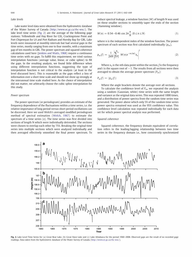
Lake water level data were obtained from the hydrometric databaseof the Water Survey of Canada (http://www.ec.gc.ca/rhc-wsc/). Thelake level time series (Fig. 2) are the average of the following gagestations: Yellowknife and Hay River for GSL, Crackingstone Point andFort Chipewyan for LA and Port Radium and Hornby Bay for GBL. Lakelevels were measured at monthly intervals but had several gaps in thetime series, mostly ranging from one to four months, with a maximumgap of ten months in GBL. The power spectrum and squared coherencecalculations used here (Jenkins and Watts, 1968) require a continuoustime series with no gaps. To fulfill this requirement, we tried variousinterpolation functions (average value, linear, or cubic spline) to fillthe gaps. In the resulting analysis, we found little difference whenusing different interpolation functions, suggesting the type ofinterpolation function is not critical to the analysis (at least to thelevel discussed here). This is reasonable as the gaps reflect a loss ofinformation over a short time scale and should not show up strongly atthe interannual time scale studied here. As the choice of interpolationdid not matter, we arbitrarily choose the cubic spline interpolation forthis study.

Power spectrum

The power spectrum (or periodogram) provides an estimate of thefrequency dependence of the fluctuations within a time series, i.e. therelative importance of long period versus short period oscillations canbe discerned. Here we used Welch's averaged modified periodogrammethod of spectral estimation (Welch, 1967) to estimate thespectrum of a time series (x). The time series was first divided intosections of length N which were individually detrended. The sectionswere chosen to overlap each other by 75%. Breaking the original timeseries into multiple sections which were analyzed individually andthen averaged effectively smoothed the final power spectrum. To

Fig. 2. Lake Level Time Series for (a) Great Bear Lake, (b) Great Slave Lake and (c) Lake Areadings. Data taken from the hydrometric database of the Water Survey of Canada (http:/

reduce spectral leakage, a window function (W) of length N was usedon these smaller sections to smoothly taper the ends of the section(Hamming window).

W nð Þ = 0:54−0:46 cos 2πnN

0≤ n≤Nð Þ ð1Þ

where n is the independent index of the window function. The powerspectrum of each section was first calculated individually (pxx),

pxx fð Þ = 12πN

∑N

n=1W nð Þe−in 2πfð Þxn

������

������

2

ð2Þ

Where xn is the nth data point within the section, f is the frequencyand i is the square root of −1. The results from all sections were thenaveraged to obtain the average power spectrum (Pxx):

Pxx fð Þ = pxx fð Þh i ð3Þ

Where the angle brackets denote the average over all sections.To calculate the confidence level of Pxx, we repeated the analysis

using a random (Gaussian, white) time series with the same lengthand variance as the original data series. This was repeated 1000 times,and a distribution of power spectra from the random time series wasgenerated. The power above which only 5% of the random time seriespower spectra remained was used as the 95% confidence value. Thisconfidence level calculation was repeated individually for each dataset for which power spectral analysis was performed.

Squared coherence

Squared coherence, the frequency domain equivalent of correla-tion refers to the leading/lagging relationship between two timeseries in the frequency domain i.e., how consistently synchronized

thabasca for the period 1960–2008. Observed gaps are the result of no recorded gage/www.ec.gc.ca/rhc-wsc/).

645S. Sarmiento, A. Palanisami / Journal of Great Lakes Research 37 (2011) 642–649

they are in terms of phase at particular timescales (Ghanbari andBravo, 2008; Von Storch and Zwiers, 1999). Squared coherenceranges in values between zero and one and measures the time-averaged phase correlation, with systems that display inconsistentphase correlation resulting in low squared coherence values (Jenkinsand Watts, 1968). High coherence values do not require highamplitude fluctuations. Squared coherence analysis has proven tobe a useful method at the Laurentian Great lakes to determine theperiods at which correlation occurs between lake level time seriesthat display variability across a broad range of periods, andteleconnection indexes (Ghanbari and Bravo, 2008). Coherence doesnot necessarily mean causality; however significant coherence valuessupport a correlation between changes in both series (Ghanbari andBravo, 2008).

To calculate the squared coherence of two time series (x and y), wefollowed the method outlined by Von Storch and Zwiers (1999).Briefly, the time series were divided into sections of length N whichwere individually detrended. The sections were chosen to overlapeach other by 75%. A Hamming window was used on the individualsections. The cross spectrum of each individual section was thencalculated (pxy):

pxy fð Þ = 12πN

∑N

n=1W nð Þe−in 2πfð Þxn

������

������∑

N

m=1W mð Þe−im 2πfð Þym

������

������ð4Þ

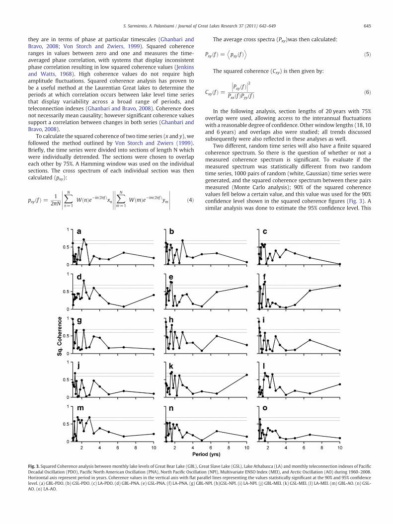
Fig. 3. Squared Coherence analysis between monthly lake levels of Great Bear Lake (GBL), GreDecadal Oscillation (PDO), Pacific North American Oscillation (PNA), North Pacific OscillatioHorizontal axis represent period in years. Coherence values in the vertical axis with flat paralevel. (a) GBL-PDO. (b) GSL-PDO. (c) LA-PDO. (d) GBL-PNA. (e) GSL-PNA. (f) LA-PNA. (g) GBL-AO. (o) LA-AO.

The average cross spectra (Pxy)was then calculated:

Pxy fð Þ = pxy fð ÞD E

ð5Þ

The squared coherence (Cxy) is then given by:

Cxy fð Þ =Pxy fð Þ���

���2

Pxx fð ÞPyy fð Þ ð6Þ

In the following analysis, section lengths of 20 years with 75%overlap were used, allowing access to the interannual fluctuationswith a reasonable degree of confidence. Other window lengths (18, 10and 6 years) and overlaps also were studied; all trends discussedsubsequently were also reflected in these analyses as well.

Two different, random time series will also have a finite squaredcoherence spectrum. So there is the question of whether or not ameasured coherence spectrum is significant. To evaluate if themeasured spectrum was statistically different from two randomtime series, 1000 pairs of random (white, Gaussian) time series weregenerated, and the squared coherence spectrum between these pairsmeasured (Monte Carlo analysis); 90% of the squared coherencevalues fell below a certain value, and this value was used for the 90%confidence level shown in the squared coherence figures (Fig. 3). Asimilar analysis was done to estimate the 95% confidence level. This

at Slave Lake (GSL), Lake Athabasca (LA) andmonthly teleconnection indexes of Pacificn (NPI), Multivariate ENSO Index (MEI), and Arctic Oscillation (AO) during 1960–2008.llel lines representing the values statistically significant at the 90% and 95% confidenceNPI. (h)GSL-NPI. (i) LA-NPI. (j) GBL-MEI. (k) GSL-MEI. (l) LA-MEI. (m) GBL-AO. (n) GSL-

646 S. Sarmiento, A. Palanisami / Journal of Great Lakes Research 37 (2011) 642–649

method of estimating confidence levels was first described byThompson (1979). To account for the effects of data gaps and thesubsequent interpolation, the same pattern of gaps which occurred inthe lake level data was forced onto the random time series used forthe Monte Carlo analysis. Including the gap/interpolation in theMonte Carlo analysis only changed the confidence level by a fewpercent. This is expected as the gaps remove information from thetime series and the subsequent simple interpolations used areunlikely to create phase correlation.

Teleconnections

The teleconnection index values used in this study were monthlystandardized anomalies. The North Pacific Index (associated with NP),is the area-weighted sea level pressure over the region 30°N–65°N,160°E–140°W; this index provides a measure of the intensity of themean wintertime Aleutian Low and was obtained from http://www.cgd.ucar.edu/cas/jhurrell/NPndex.html.

The PNA Index represents amode of low-frequency variability in thenorthern hemisphere. The PNApositive phase is characterized by higherthan a normal ridge over the Rockies and a deeper than normal troughover the Aleutian area and the eastern United States (Yin, 1994). Thepositive phase is associated with a meridional upper-level flow and thenegative phasewith a zonal upper-levelflow. The PNA characterizes the700 mb atmospheric flow and is an important component in under-standing the low-frequency variability of the mean tropospheric flowover North America (Quiring, 2010). The PNA Index derived from theWallace and Gutzler (1981) method was obtained from http://www.jisao.washington.edu/data_sets/pna/pna19482009.

The PDO Index is based on the pattern of Sea-Surface Temperature(SST) in the North Pacific Ocean poleward of 20°N. PDO representsinterdecadal oscillations with events that could persist 20 to 30 yearsunlike El Niño which last between 6 and 18 months; furthermore, PDOismore influential in theNorth Pacific of NorthAmericawhereas ElNiñoeffect is stronger in the tropics (Mantua and Hare, 2002) The PDO datawere obtained from http://jisao.washington.edu/pdo/PDO.latest.

El Niño is the periodic warming in sea-surface temperatures acrossthe central and east-central equatorial Pacific. Multiple indexes havebeen developed to describe the El Niño Southern Oscillation (ENSO)and due to its complexity, different areas are better characterized byspecific indexes.

The Multivariate ENSO Index (MEI) was chosen since it betterreflects the coupled ocean–atmosphere system at a more global scale(Wolter and Timlin, 1993; Wolter and Timlin, 1998). This index isbased on six observed variables over the tropical Pacific: sea-levelpressure, zonal and meridional components of the surface wind, sea-surface temperature, surface air temperature, and total cloudinessfraction of the sky (Wolter and Timlin, 1998). The MEI data wasobtained from: http://www.esrl.noaa.gov/psd/people/klaus.wolter/MEI/mei.html.

The Arctic Oscillation (AO) is the dominant pattern of non-seasonalsea-level pressure (SLP) variations north of 20°N and is calculated by

Fig. 4. Power Spectrum Analysis of lake levels of (a) Great Bear Lake, (b) Great Slave Lake anstatistically significant at the 95% confidence level.

projecting the 1000 mb height anomalies poleward of 20°N onto theloading pattern of the AO. The AO index is important since it describesthe pressure over the arctic regions. (Thompson and Wallace, 1998;Wang and Ikeda, 2000). Lower than normal pressure over the Arcticleads to stronger westerlies in the upper atmosphere and subsequentwarm phases, while the opposite is the case for the cold phase (http://jisao.washington.edu/ao/). AO data was taken from (http://www.cpc.ncep.noaa.gov/products/precip/CWlink/daily_ao_index/ao.shtml).

Results and discussion

We begin by looking at the squared coherence between the lakesof the MRB and several different teleconnections at the interannualand interdecadal periods (Fig. 3). The squared coherence wascalculated as in Eq. 6 where f is defined as 1/period. The direct effector lake level response to a given teleconnection was assumed to takeplace at the periods whose coherence values were significant at the90% confidence level or higher. In the 1.1–3 year period range, manyof the squared coherence analyses displayed periods of significantcoherence. In particular, GSL and LA had an almost identical responseto PNA at 1.17, 1.53 and 1.66 year periods (Figs. 3e, f). Similarly, ElNiño (MEI) also showed significant squared coherence values withGSL and LA levels at the 1.1–3 year timescale, although the El Niño(MEI) coherence values were lower and the statistically significantperiods were not identical between the two lakes as it was for PNA(Figs. 3e, f, k, l). Repeating this analysis using annual values instead ofmonthly values for the time series displays a similar trend of 1.1–3 year phase correlation (See Fig A.1 in the appendix).

For the ten-year period, the results were clearer. Only PNA and ElNiño (MEI) displayed significant squared coherence values at theinterdecadal timescale. Once again, the PNA squared coherenceshowed up strongly in the southern two lakes (GSL and LA), whereasEl Niño (MEI) was only significant in GSL.

The significant phase correlation found at the 1.1–3 year periodand the 10-year period led to the next question; how important werethe lake level fluctuations at these timescales? To answer this, weused power spectral analysis. The power spectra of all three lakes(Fig. 4) showed greater fluctuation with longer periods, with the 10-year period amplitude fluctuations roughly five times larger than thefluctuations at the 1.1–3 year period. Therefore, 1.1–3 year fluctua-tions were not as important as the 10-year fluctuations, but were stillsignificant.

The power spectra of the teleconnections were also analyzed(Fig. 5). Over the timescales studied, no clear trend in fluctuationamplitude versus period was found. As expected, El Niño MEI showedenhanced fluctuations over a 3–5 year period and PDO showed astrong long period amplitude fluctuation. In contrast, the otherteleconnections were relatively flat with period over the 1.1–10 yeartime scale.

Squared coherence was also used to examine temporal correlationbetween the different lakes of the MRB (Fig. 6). The squaredcoherence was again calculated as in Eq. 6. GSL and LA showed a

d (c) Lake Athabasca for the period 1960–2008. The horizontal line represent the values

Fig. 5. Power Spectrum Analysis of teleconnection indexes for (a) Pacific Decadal Oscillation—PDO, (b) Pacific North American Oscillation—PNA, (c) North Pacific Index—NP,(d) Multivariate ENSO Index—MEI and (e) Arctic Oscillation—AO, for the period 1960–2008. The horizontal line represent the values statistically significant at the 95% confidencelevel.

647S. Sarmiento, A. Palanisami / Journal of Great Lakes Research 37 (2011) 642–649

very significant coherence (N95% confidence) over the 3.5–10 yearperiod. For the 1.1–3.5 year period, the coherence became morevariable, but still significant. In contrast, GSL and GBL showed nosignificant coherence over the 1.1–10 year time scale.

Interdecadal (10 year period)

The squared coherence analysis found significant interdecadalcorrelations between the southern two lakes (GSL and LA) and PNA(Figs. 3e, f). As the 10-year period lake level fluctuations wererelatively large (Fig. 4), this timescale was an important player in theoverall lake level variability. To look for the origin of the 10-yearperiod coherence we examined the power spectrum of PNA (Fig. 5b)but the PNA power spectrum revealed no particularly strongfluctuations at the 10-year period. Apparently, 10-year period PNAfluctuations have a disproportionately large coherence with the lakelevels in the southern half of the MRB. That the two southern lakes

Fig. 6. Squared Coherence between lake levels of (a) Great Slave Lake and LakeAthabasca and (b) Great Slave Lake and Great Bear Lake. LA sub-basin is part of thelarger GSL sub-basin. Coherence values in the vertical axis with flat parallel linesrepresenting the values statistically significant at the 90% and 95% confidence level.

gave a similar response is not unexpected as both lakes are part of thesame catchment, with LA outflow feeding into the Peace River whichtogether form the Slave River, the main inflow to GSL.

El Niño (MEI) also gave a significant interdecadal squaredcoherence with GSL, but not with LA. One possible explanationstems from differences in El Niño's influence on the precipitationpatterns of the Peace River sub-basin as compared to the AthabascaRiver sub-basin (MAGS, 2005). Given the 10-year timescale, PDO mayalso be expected to play a role in the interdecadal lake levels.Surprisingly, PDO displayed little coherence with any of the lakes atthis timescale, despite having sizable interdecadal fluctuations(Fig. 5a). Whatever influence PDO has on the basin lake levels cannotbe simply explained by phase correlation.

In the LaurentianGreat Lakes, Ghanbari and Bravo (2008) found thatboth PNA and PDOwere significantly coherent on the interdecadal timescale. As both theMRB and Laurentian basins arewithin the four centersof geopotential high anomalies that define the PNA index, a similarresponse of both basins to PNA could be expected. PDO has also beencorrelated with flow out of the Liard sub-basin (which drains into theMackenzie River) byBurn et al. (2004), so the lack of coherencebetweenMRB lake levels and PDO is a non-trivial interaction.

Intriguingly, muskrat populations have also been found to have an11 year cycle (Timoney et al., 1997). A connection between thismuskrat cycle and the decadal correlations found here is possible, buta squared coherence analysis of the muskrat population oscillationswith the teleconnections has not yet been performed. As muskrattrapping is an important economic activity for native inhabitants ofthe MRB, correlation of muskrat populations with teleconnectionscould aid in management of this resource.

Long inter-annual (3–7 year period)

In the 3–7 year timescale, no significant coherence was foundbetween any lake with any teleconnection. This is somewhatsurprising as coherence was found at both longer and shorter periods.This lack of significant coherence was not due to small fluctuations ofthe teleconnections; all of the teleconnections studied here havesubstantial fluctuations at the 3–7 year timescale (Fig. 5). It is possiblethat nonlinear interference between different teleconnections wasobscuring the squared coherence signal of any particular teleconnec-tion, resulting in low coherence. Another simpler possibility is thatteleconnections were not strongly connected with MRB lake levels at

648 S. Sarmiento, A. Palanisami / Journal of Great Lakes Research 37 (2011) 642–649

these timescales. In the Laurentian great lakes, ENSO was found to bestrongly correlated with lake levels at this timescale. However, this isnot unexpected as the effects of ENSO are known to be regiondependent (Redmond and Koch, 1991; Timoney et al., 1997).

Short inter-annual (1.1 to 3 year period)

Across the MRB, many of the teleconnections examined had asignificant squared coherence in the 1.1–3 year periods. At this timescale, the noise due to the monthly variations in the time series mustbe considered. The squared coherence looks at phase correlationbetween the time series, and a statistically significant coherencemeans the fluctuations between time series (even if they are due to‘noise’) must be phase correlated. It is unlikely that random noisewould be phase correlated between two different time series (thispoint is the foundation of the Monte Carlo confidence intervalcalculation described previously). Additionally, repeating the analysiswith annual values instead of monthly values gave similar trends(appendix), suggesting the correlations were not due to noise in themonthly values. The preponderance of significant coherence values atthis timescale (in contrast to the lack of coherence generally found atthe 3–7 year periods) was striking; consideration of these teleconnec-tions could aid in short inter-annual lake level prediction. While thelake level fluctuations at this time scale were only ~20% as large as theinterdecadal fluctuations (Fig. 4), they were still a nontrivialcomponent of the overall lake level fluctuation.

The squared coherence between the AO and GBL was significant at1.53, 1.66, 2.0, 2.8 year periods (Fig. 3m). The lack of significantcoherence between AO and GSL and LA (Fig. 3n, o) indicates the effectof this oscillation was restricted to the northern part of the MRB.

El Niño (MEI), on the other hand, showed significant coherencewith the southern half of the MRB with several periods within a 1.1–3 year time scale (Figs. 3k,l). As several agencies put forwardpredictions of ENSO up to 6 months in advance (Piechota et al.,2006) this correlation may be especially suitable as an aid inforecasting of GSL and LA lake levels on this timescale or forcalibration of MRB hydrological models. In contrast, the El NiñoMEI-GBL coherence was comparatively weak (Fig. 3j). This lack ofcoherence supports the interpretation of a weak El Niño effect in thenorthern part of the basin.

NP, which represents the intensity of the wintertime Aleutian Low,is the teleconnection with the greatest number of periods that weresignificantly in coherence with the levels of GBL, GSL and LA (Figs. 3g,h, i). Those periods differ for GBL (1.33, 1.43, 2.2 years), GSL (1.53,1.66, 2.0, 2.85 years) and LA (1.11 and 1.66 years) suggesting a perioddependent lake response to the Aleutian Low across the MRB.

Flow regulation effects

Human influence on inflow/outflow from the lakes can affectcorrelations between climate variability and lake levels. The mostsignificant contribution in this regard is from theW.A.C. Bennett Dam,which has regulated the Peace River since 1967 and impact waterlevels in Great Slave Lake. However, a daily water balance model forGSL for the period 1964–1998 Gibson et al. (2006) found that theprimary driving force behind lake level fluctuation to be climate-driven precipitation variability in the Peace-Athabasca basin and notregulation. In this study, GSL water level at any given year wasestimated using Peace-Athabasca basin precipitation data from thatyear and the prior 2 years (coefficient of determination; r2=0.52).Their findings suggest that for periods larger than 3 years, GSL waterlevel can be predicted by precipitation in the Peace-Athabasca basin(although anthropogenic effects may still play a significant role).

To investigate the temporal effects of the dam, we examined thesquared coherence of the lake levels between LA and GSL (Fig. 6a)with the rationale that Bennett dam regulation should have a stronger

effect on GSL than LA because of the continuous flow of the PeaceRiver into Great Slave Lake via the Slave River. For four year periodsand longer, the two lakes had a highly significant phase correlation,suggesting dam regulation had little effect on the GSL lake levelfluctuations at this timescale. However for 3.5 year periods andshorter, the coherence was smaller and more variable. Dam activitymay play a role in this reduced phase correlation.

Conclusions

At the interdecadal timescale, relatively large lake level fluctua-tions were found in the three largest lakes of the MRB. PNA wassignificantly coherent at the interdecadal timescale with the lake levelfluctuations in the southern half of the basin and may have predictivevalue in this regard. Coherence with El Nino also occurred at thistimescale, but the effect was latitude dependent. At the 1.1–3 yeartimescales, lake level fluctuations were correlated with a number ofteleconnections, but the relationship was latitude and perioddependentwhich complicated the use of teleconnections as predictivetools at this timescale. The lake levels of GSL and LA in the southernhalf of the basin were found to be strongly coherent at the 4–10 yeartimescale, suggesting they were strongly linked, whereas thecoherence of GSL with GBL was weak over all timescales studied.Since Great Bear Lake is not hydrologically connected to LakeAthabasca and Great Slave Lake basins, this lack of coherence withGBL is expected.

Supplementarymaterials related to this article can be found onlineat doi:10.1016/j.jglr.2011.08.002.

References

Bonsal, B.R., Prowse, T.D., 2003. Trends and variability in spring and autumn 0 degreesC-isotherm dates over Canada. Clim. Chang. 57, 341–358.

Bonsal, B.R., Shabbar, A., Higuchi, K., 2001. Impacts of low frequency variability modeson Canadian winter temperature. Int. J. Climatol. 21, 95–108.

Bonsal, B.R., Prowse, T.D., Duguay, C.R., Lacroix, M.P., 2006. Impacts of large-scaleteleconnections on freshwater-ice break/freeze-up dates over Canada. J. Hydrol.330, 340–353.

Brown, R., Derksen, C., Wang, L., 2007. Assessment of spring snow cover durationvariability over northern Canada from satellite datasets. Remote. Sens. Environ.111, 367–381.

Burn, D.H., Cunderlik, J.M., Pietroniro, A., 2004. Hydrological trends and variability inthe Liard River basin. Hydrol. Sci. 49 (1), 53–67.

Cohen, S.J., 1997. Mackenzie Basin Impact Study (MBIS). In: Cohen, S.J. (Ed.), Vancouver.Cohn, B.P., Robinson, J.E., 1976. Forecast model for great lakes water levels. J. Geol. 84,

455–465.Duguay, C.R., Lafleur, P.M., 2003. Determining depth and ice thickness of shallow sub-

Arctic lakes using space-borne optical and SAR data. Int. J. Remote. Sens. 24,475–489.

Duguay, C.R., Prowse, T.D., Bonsal, B.R., Brown, R.D., Lacroix, M.P., Menard, P., 2006.Recent trends in Canadian lake ice cover. Hydrol. Process. 20, 781–801.

Evans, M.S., 2000. The large lake ecosystems of northern Canada. Aquat. Ecosyst. Heal.Manag. 3, 65–79.

Ghanbari, R.N., Bravo, H.R., 2008. Coherence between atmospheric teleconnections,Great Lakes water levels, and regional climate. Adv. Water Res. 31, 1284–1298.

Gibson, J.J., Prowse, T.D., Peters, D.L., 2006. Hydroclimatic controls on water balance andwater level variability in Great Slave Lake. Hydrol. Process. 20, 4155–4172.

Herdendorf, C.E., 1982. Large lakes of the world. J. Great Lakes Res. 8, 379–412.Howell, S.E.L., Brown, L.C., Kang, K.K., Duguay, C.R., 2009. Variability in ice phenology on

Great Bear Lake and Great Slave Lake, Northwest Territories, Canada, fromSeaWinds/QuikSCAT: 2000–2006. Remote. Sens. Environ. 113, 816–834.

Ioannidou, L., Yau, M.K., 2008a. Climatological analysis of the Mackenzie River Basinanticyclones: structure, evolution and interannual variability. In: Woo, M.K. (Ed.),Cold Region Atmospheric and Hydrologic Studies. Springer, Berlin, pp. 51–60.

Ioannidou, L., Yau, M.K., 2008b. A climatology of the Northern Hemisphere winteranticyclones. J. Geophys. Res. Atmos. 113 17 pp.

Jenkins, G.M., Watts, D.G., 1968. Spectral analysis and its applications. Holden Day.Kistler, R., Kalnay, E., Collins, W., Saha, S., White, G., Woollen, J., Chelliah, M., Ebisuzaki,

W., Kanamitsu, M., Kousky, V., van den Dool, H., Jenne, R., Fiorino, M., 2001. TheNCEP-NCAR 50-year reanalysis: monthly means CD-ROM and documentation. Bull.Am. Meteorol. Soc. 82, 247–267.

Lackmann, G.M., Gyakum, J.R., Benoit, R., 1998. Moisture transport diagnosis of awintertime precipitation event in the Mackenzie River basin. Mon. Weather. Rev.126, 668–691.

Latifovic, R., Pouliot, D., 2007. Analysis of climate change impacts on lake ice phenologyin Canada using the historical satellite data record. Remote. Sens. Environ. 106,492–507.

649S. Sarmiento, A. Palanisami / Journal of Great Lakes Research 37 (2011) 642–649

Lenormand, F., Duguay, C.R., Gauthier, R., 2002. Development of a historical ice databasefor the study of climate change in Canada. Hydrol. Process. 16, 3707–3722.

Lick, W., 1982. The transport of contaminants in the Great Lakes. Annu. Rev. EarthPlanet. Sci. 10.

Magnuson, J.J., Robertson, D.M., Benson, B.J., Wynne, R.H., Livingstone, D.M., Arai, T.,Assel, R.A., Barry, R.G., Card, V., Kuusisto, E., Granin, N.G., Prowse, T.D., Stewart, K.M.,Vuglinski, V.S., 2000. Historical trends in lake and river ice cover in the NorthernHemisphere. Science 289, 1743–1746.

MAGS, 2005. Final report of theMackenzie GEWEX Study (MAGS). In: Di Cenzo, P. (Ed.),Proceedings of the final (11th) annual scientific meeting. GEWEX, Ottawa, CA.

Mantua, N.J., Hare, S.R., 2002. The Pacific decadal oscillation. J. Oceanogr. 58, 35–44.Mantua, N.J., Hare, S.R., Zhang, Y., Wallace, J.M., Francis, R.C., 1997. A Pacific interdecadal

climate oscillation with impacts on salmon production. Bull. Am. Meteorol. Soc. 78,1069–1079.

MRBB, 2003. State of the Aquatic Ecosystem Report 2003. In: Secreatariat, M. (Ed.), FortSmith, NT.

NOAA, 2009. Bering Climate. http://www.beringclimate.noaa.gov/index.html 2009.Piechota, T.C., Garbrecht, J.D., Schneider, J.M., 2006. Climate variability and climate change.

In: Garbrecht, J.D., Piechota, T.C. (Eds.), Climate Variations, climate change and waterresources engineering. ASCE, American Association of Civil Engineers, Reston, VA.

Pietroniro, A., Leconte, R., Toth, B., Peters, D.L., Kouwen, N., Conly, F.M., Prowse, T., 2006.Modelling climate change impacts in the Peace and Athabasca catchment anddelta: III — integrated model assessment. Hydrological Processes 20, 4231–4245.doi:10.1002/hyp.6428.

Prowse, T.D., Beltaos, S., Gardner, J.T., Gibson, J.J., Granger, R.J., Leconte, R., Peters, D.L.,Pietroniro, A., Romolo, L.A., Toth, B., 2006. Climate change, flow regulation and land-use effects on the hydrology of the Peace-Athabasca-Slave system; Findings from theNorthern Rivers Ecosystem Initiative. Environ. Monit. Assess. 113, 167–197.

Quiring, S.M., 2010. Class notes. Texas A&M University.Redmond, K., Koch, R., 1991. Surface climate and streamflow variability in the Western

United States and their relationship to large-scale circulation indices. WaterResour. Res. 27, 2381–2399.

Rouse, W.R., Oswald, C.J., Binyamin, J., Spence, C.R., Schertzer, W.M., Blanken, P.D.,Bussieres, N., Duguay, C.R., 2005. The role of northern lakes in a regional energybalance. J. Hydrometeorol. 6, 291–305.

Rouse,W., Blanken, P., Duguay, C., 2008. Climate–lake interactions. In:Woo, M.-K. (Ed.),Cold Region Atmospheric and Hydrologic Studies. The Mackenzie GEWEXExperiment. Springer, Berlin, pp. 139–160.

Schertzer, W.M., Rouse, W.R., Blanken, P.D., Walker, A.E., 2003. Over-lake meteorologyand estimated bulk heat exchange of Great Slave Lake in 1998 and 1999.J. Hydrometeorol. 4, 649–659.

Serreze, M.C., Walsh, J.E., Chapin, F.S., Osterkamp, T., Dyurgerov, M., Romanovsky, V.,Oechel, W.C., Morison, J., Zhang, T., Barry, R.G., 2000. Observational evidence ofrecent change in the northern high-latitude environment. Clim. Chang. 46, 159–207.

Smirnov, V.V., Moore, G.W.K., 1999. Spatial and temporal structure of atmosphericwater vapor transport in the Mackenzie River basin. J. Clim. 12, 681–696.

Szeto, K.K., Stewart, R.E., Yau, M.K., Gyakum, J., 2007. Northern tales — a synthesis ofMAGS atmospheric and hydrometeorological research. Bull. Am. Meteorol. Soc. 88,1411–1425.

Thompson, R., 1979. Coherence significance levels. J. Atmos. Sci. 36 (10), 2020–2021.Thompson, D.W.J., Wallace, J.M., 1998. The Arctic Oscillation signature in the wintertime

geopotential height and temperature fields. Geophys. Res. Lett. 25, 1297–1300.Timoney, K., 1995. Peace like a River: ecological studies and restoration in Wood

Buffalo National Park. In: Herman, T.B., et al. (Ed.), Ecosystem Monitoring andProtected Areas. Science and Management of Protected Areas Association, Halifax,pp. 490–500.

Timoney, K., Peterson, G., Fargey, P., Peterson, M., 1997. Spring ice-jam flooding of thePeace-Athabasca Delta: evidence of a climatic oscillation. Clim. Chang. 35, 463–483.

Trenberth, K.E., 1990. Recent observed interdecadal climate changes in the Northern-Hemisphere. Bull. Am. Meteorol. Soc. 71, 988–993.

Trenberth, K.E., Hurrell, J.W., 1994. Decadal atmosphere–ocean variations in the Pacific.Clim. Dyn. 9, 303–319.

Von Storch, H., Zwiers, F.W., 1999. Statistical analysis in climate research. CambridgeUniversity Press, Cambridge.

Wallace, J.M., Gutzler, D.S., 1981. Teleconnections in the geopotential height fieldduring the Northern Hemisphere winter. Mon. Weather. Rev. 109, 784–812.

Wang, J., Ikeda, M., 2000. Arctic oscillation and Arctic sea-ice oscillation. Geophys. Res.Lett. 27, 1287–1290.

Welch, P.D., 1967. Use of fourier transform for estimation of power spectra— a methodbased on time averaging over short modified periodograms. IEEE Trans. AudioElectroacoust. 15 (2), 70–73.

Wolter, K., Timlin, M.S., 1993. Monitoring ENSO in COADS with a seasonally adjustedprincipal component index. Proc. of the 17th Climate Diagnostics Workshop.NOAA/NMC/CAC, NSSL, Oklahoma Clim. Survey, CIMMS and the School of Meteor,Norman, OK.

Wolter, K., Timlin, M.S., 1998. Measuring the strength of ENSO — how does 1997/98rank? Weather 53, 315–324.

Yin, Z.Y., 1994. Reconstruction of the winter Pacific-North American teleconnection patternduring 1895–1947 and its application in climatological studies. Clim. Res. 4, 79–94.

Zdan, T., Dobell, R., de Bastiani, P., Cleveland, R., Hanna, A., 1997. Round table # 4:maintenance of infrastructure. In: Cohen, S.J. (Ed.), Mackenzie Basin Impact Study(MBIS). Environment Canada.