Embed Size (px)
Citation preview
Numerically Modelling Stochastic Lie Transport in Fluid Dynamics∗
Colin Cotter†1, Dan Crisan‡1, Darryl D. Holm§1, Wei Pan¶1, and Igor Shevchenko‖1
1Department of Mathematics, Imperial College London
September 28, 2018
Abstract
We present a numerical investigation of stochastic transport in ideal fluids. According to Holm (Proc Roy
Soc, 2015) and Cotter et al. (2017), the principles of transformation theory and multi-time homogenisation,
respectively, imply a physically meaningful, data-driven approach for decomposing the fluid transport veloc-
ity into its drift and stochastic parts, for a certain class of fluid flows. In the current paper, we develop new
methodology to implement this velocity decomposition and then numerically integrate the resulting stochastic
partial differential equation using a finite element discretisation for incompressible 2D Euler fluid flows. The
new methodology tested here is found to be suitable for coarse graining in this case. Specifically, we perform
uncertainty quantification tests of the velocity decomposition of Cotter et al. (2017), by comparing ensembles of
coarse-grid realisations of solutions of the resulting stochastic partial differential equation with the “true solu-
tions” of the deterministic fluid partial differential equation, computed on a refined grid. The time discretisation
used for approximating the solution of the stochastic partial differential equation is shown to be consistent. We
include comprehensive numerical tests that confirm the non-Gaussianity of the stream function, velocity and
vorticity fields in the case of incompressible 2D Euler fluid flows.
Contents
1 Introduction 2
2 The two-dimensional incompressible flow equations 6
2.1 Deterministic version . . . . . . . . . . . . . . . . . . . . . . . . . . . . . . . . . . . . . . . . . . . . . . . . 6
2.1.1 Numerical implementation . . . . . . . . . . . . . . . . . . . . . . . . . . . . . . . . . . . . . . . . . 6
2.2 Stochastic version . . . . . . . . . . . . . . . . . . . . . . . . . . . . . . . . . . . . . . . . . . . . . . . . . . 8
2.2.1 Numerical implementation . . . . . . . . . . . . . . . . . . . . . . . . . . . . . . . . . . . . . . . . . 10
2.2.2 Consistency of the numerical method for the SPDE . . . . . . . . . . . . . . . . . . . . . . . . . . 12
3 Calibration of the correlation eigenvectors 16
3.1 Methodology . . . . . . . . . . . . . . . . . . . . . . . . . . . . . . . . . . . . . . . . . . . . . . . . . . . . . 16
3.2 Numerical experiments . . . . . . . . . . . . . . . . . . . . . . . . . . . . . . . . . . . . . . . . . . . . . . . 17
3.2.1 Fine grid PDE solution and its coarse graining . . . . . . . . . . . . . . . . . . . . . . . . . . . . 17
∗This work was partially supported by the EPSRC Standard Grant EP/N023781/1.†[email protected]‡[email protected]§[email protected]¶[email protected]‖[email protected]
1
arX
iv:1
801.
0972
9v2
[ph
ysic
s.fl
u-dy
n] 2
6 Se
p 20
18

3.2.2 Lagrangian trajectories and estimating the correlation eigenvectors . . . . . . . . . . . . . . . . 18
3.2.3 SPDE ensemble and SPDE initial conditions . . . . . . . . . . . . . . . . . . . . . . . . . . . . . 19
3.2.4 SPDE uncertainty quantification . . . . . . . . . . . . . . . . . . . . . . . . . . . . . . . . . . . . . 23
3.2.5 Additional statistical tests . . . . . . . . . . . . . . . . . . . . . . . . . . . . . . . . . . . . . . . . 28
4 Conclusion and future work 31
1 Introduction
A fundamental challenge in observational sciences, such as weather forecasting and climate change prediction, is
the modelling of measurement error and uncertainty due, for example, to unknown or neglected physical effects,
and incomplete information in both the data and the formulations of the theoretical models for prediction. To meet
this challenge, new types of dynamical parameterisations, called Data Driven Models have been developing recently
for the observational sciences. Data-driven models accommodate uncertainty in observational science, by making
predictions of both the values of the expected future measurements and of their uncertainties, or variabilities, based
on input from measurements and statistical analysis of the initial data.
Such predictions are made in a probabilistic sense. They may also use data assimilation to take into account
the time integrated information obtained from the data being observed along the solution path during the forecast
interval as “in flight corrections”. Data assimilation is a term used mainly in the computational geoscience com-
munity, and refers to methodologies that combine past knowledge of a system in the form of a numerical model
with new information about that system in the form of observations of that system. It is a major component
of Numerical Weather Prediction, where it is used to improve forecasting, reduce model uncertainties and adjust
model parameters. To reduce the uncertainty, a stochastic feedback loop between the model and the data may be
introduced, through which assimilation of more data during the prediction interval will decrease the uncertainty of
the forecasts based on the initial data, by selecting the likely paths as more observational data is accrued. This is
the basis of the so-called ensemble data assimilation which uses a set of model trajectories that are intermittently
updated according to data. The availability for several years of large grid computing systems has made ensem-
ble data assimilation increasingly popular. Ensemble data assimilation can use particle filters1 as a basis for the
uncertainty reduction.
Thus, in modern observational science, predictive dynamics meets: (i) observation error, (ii) incomplete in-
formation, (iii) uncertainty, (iv) resolution errors in numerical simulations and (v) data assimilation. In the new
science of data-driven modelling, all four of these endeavours should be placed into the same framework. As a
minimum requirement, the framework for the introduction of noise should preserve the fundamental mathematical
structure of the deterministic model. The geometric mechanics approach that we take here is designed to preserve
the fundamental structure of fluid dynamics, which is based on the theory of transformations by smooth invertible
maps.
Our approach introduces a new type of stochasticity – called Stochastic Lie Transport (SLT) – that has been
designed specifically for fluid dynamics, based on transformation theory and geometric mechanics. Instead of trying
to predict the effects of what cannot be resolved in each case by going to even higher resolution, SLT uses observed
spatial correlation data to model the effects of the uncertainty as spatially correlated stochastic transport.
Properties of Stochastic Lie Transport in Ideal Fluid Dynamics
Stochastic Lie Transport (SLT) for ideal fluid dynamics was first derived in Holm [2015] by applying transformation
theory from geometric mechanics (based on the smooth invertible Lagrange-to-Euler map) to the Hamilton varia-
tional principle for the equations of ideal fluid motion. SLT also follows from Newton’s Law of Motion, provided one
includes the stochastic Lagrange-to-Euler transformation of the reference coordinate basis under the fluid flow, as
shown in Crisan et al. [2017]. In addition, homogenisation theory shows that SLT can be regarded as a true decom-
1See Beskos et al. [2017] for a new approach for handling high dimensional models using particle filters.
2
position of the deterministic solution for the fluid velocity into a mean flow and rapid fluctuations in velocity around
the mean Cotter et al. [2017]. Via homogenisation theory, the rapid velocity fluctuations rigorously transform into
a sum of stochastic vector fields, as in equation (1.2), in the limit as the fluctuation frequency increases.
As a true decomposition of the solution, the analytical properties of the SLT fluid model should not differ from
those of the corresponding deterministic fluid equations. This property was proven to hold for the 3D SLT Euler
fluid equations in Crisan et al. [2017]. In particular, the solutions of the 3D SLT Euler fluid equations (1.1) derived
in Holm [2015] are shown in Crisan et al. [2017] to possess local-in-time existence and uniqueness, as well as to
satisfy a Beale-Kato-Majda criterion for blow-up, corresponding to the same properties as for the deterministic 3D
Euler fluid equations Beale et al. [1984].
In summary, SLT is a new type of stochasticity, designed to account for the effects of unresolved fluid degrees
of freedom, such as turbulence, on the resolved scale dynamics of fluid flows. In SLT, the noise multiplies both the
solution and the spatial gradient of the solution; so its influence tends to increase as the gradients of the solution
increase. The additional Lie transport terms in SLT turn out to be necessary to complete the Stochastic Kelvin
Circulation Theorem. Thus, in the SLT approach, the Eulerian fluid equations acquire the additional Stratonovich
stochastic transport vector field seen in equation (1.2), which leads to the Kelvin Circulation Theorem in (1.4).
These additional stochastic Lie transport terms do not appear in other theories, such as Mikulevicius and Rozovskii
[2004] and Memin [2014]. The present paper will demonstrate how to use SLT as a means of performing both
uncertainty quantification and account for the resolution error in numerical simulations by the following steps, see
Section 3.1:
• Simulate Lagrangian trajectories moving with velocity described by a deterministic PDE which we assume
can be accurately approximated on a fine grid. Call these the fine grid trajectories.
• Simulate Lagrangian trajectories moving with a spatially-filtered velocity on a coarse grid. Call these the
coarse grid trajectories.
• Calculate the differences between the fine grid trajectories and the coarse grid trajectories over non-overlapping
time intervals, which are then used to estimate the velocity-velocity correlation tensors.
• The estimated velocity-velocity correlation tensors are substituted into the Euler stochastic PDE with Lie
transport noise to perform uncertainty quantification analysis.
The Interaction Between Noise and Transport Mechanisms in Ideal Fluids
Our aim in this paper is to investigate the interaction between noise and transport in ideal fluids using the framework
of geometric mechanics, Marsden and Ratiu [1999]; Holm [2011]; Holm et al. [2009]. The understanding of transport
mechanisms in fluid dynamics is at the core of some of the main open problems in mathematics and physics. The
introduction of random perturbations into the fluid equations can be expected to profoundly influence the properties
of fluid transport and thereby raise many open questions. For a mathematical review of the literature and recent
progress on the interaction between noise and transport in the vorticity equation for 2D ideal incompressible fluids,
see Brzezniak et al. [2016].
A variational approach to the full theory of stochastic ideal fluid dynamics in 3D was derived in Holm [2015],
by using transformation theory from geometric mechanics based on the Lagrange-to-Euler map for stochastic La-
grangian particle trajectories. Its analytical properties have been investigated in Crisan et al. [2017] for the particular
case of the 3D stochastic Euler equation for incompressible fluid flow, divu = 0, given by
0 = (d +Ldyt)(ω ⋅ dS) = (dω − curl (dyt ×ω)) ⋅ dS , (1.1)
for the Eulerian vorticity 2-form ω ⋅ dS = d(u ⋅ dx) = (curlu) ⋅ dS, which is Lie transported by the Stratonovich
stochastic vector field dyt corresponding to the following stochastic process,
dyt = u(yt, t)dt +∑iξi(yt) dW
it . (1.2)
3
Here, d represents stochastic differentiation and the second term in (1.2) constitutes cylindrical Stratonovich noise,
in which the amplitude of the noise depends on space, but not time. In Ito form, (1.2) is written as
dyt = u(yt, t)dt +∑iξi(yt)dW
it +
1
2∑i
(ξi(yt) ⋅ ∇)ξi(yt)dt .
For an extension of this method to include non-stationary correlation statistics, see Gay-Balmaz and Holm [2018].
In the case of 2D planar incompressible fluid motion, the vorticity has only one component, denoted as q, and
equation (1.1) reduces to
0 = (d +Ldyt)q = dω + dyt ⋅ ∇q . (1.3)
For in-depth treatments of cylindrical noise, see Pardoux [2007]; Schaumloffel [1988]. In our case, the vectors
ξi(x), i = 1,2, . . . ,N , appearing in the stochastic vector field in (1.2) comprise N prescribed, time independent,
divergence free vectors which are to be obtained from data. That is, we incorporate SLT into fluid dynamics as a
Data–Driven Model. For example, the ξi(x) may be determined as Empirical Orthogonal Functions (EOFs), which
are eigenvectors of the velocity-velocity correlation tensor for a certain measured flow with stationary statistics,
see Hannachi et al. [2007]; Hannachi [2004]. As discussed below, the ξi(x) in equation (1.2) may also be obtained
numerically by comparisons of Lagrangian trajectory simulations at fine and coarse space and time scales.
The introduction of cylindrical Stratonovich noise into Euler’s fluid equation by using its variational and Hamil-
tonian structure has introduced an additional, stochastic vector field ∑i ξi(x) dWit into equation (1.2) which
augments the Lie transport in equation (1.1). This is natural, because the essence of Euler fluid dynamics is Lie
transport, see Holm et al. [1998]. In particular, equation (1.1) produces a natural Kelvin Circulation Theorem of
the form
d∮c(dyt)
u ⋅ dx = ∮c(dyt)
(d +Ldyt)(u ⋅ dx) = ∫∫∂S=c(dyt)
(d +Ldyt)(ω ⋅ dS) = 0 , (1.4)
where c(dyt) is a closed fluid loop moving with the stochastic vector field velocity dyt.
Other 3D stochastic Euler fluid equations have been derived by different methods in Mikulevicius and Rozovskii
[2004] and Memin [2014]. However, those other derivations have produced equations which differ from (1.1) in their
stochastic transport terms and consequently do not admit the Kelvin Circulation Theorem in (1.4).
Remark 1 (Kelvin’s Circulation Theorem). From the viewpoint of geometric mechanics, Kelvin’s Circulation
Theorem (1.4) is always a fundamental property in fluid dynamics. It is the relation obtained via Noether’s
Theorem from invariance of Eulerian fluid variables under smooth invertible transformations of the Lagrangian
particle labels. This invariance is called relabelling symmetry. If one starts with the Lagrange-to-Euler map, this
invariance yields a momentum map which satisfies Kelvin’s Circulation Theorem. Even when the Lagrange-to-
Euler map is stochastic, as in equation (1.2), the relabelling symmetry is still maintained, and this invariance
implies a stochastic Kelvin’s Circulation Theorem. In the stochastic case, the closed circulation loop around which
one integrates in Kelvin’s theorem follows the flow lines of the stochastic Lagrangian paths, and it remains a loop
because the stochastic Lagrange-to-Euler map is still a diffeomorphism. Thus, Kelvin’s Circulation Theorem has
the same geometric transport interpretation in both the deterministic and stochastic cases. This preservation of
the Kelvin Circulation Theorem interpretation for stochastic fluid dynamics is unique to the present approach. The
same interpretation also applies to the equivalent Hamiltonian formulation of these equations.
The main content of the paper
The rest of the paper is structured as follows. Section 2 describes the damped and forced deterministic system and
the numerical methodology we use to solve the system on a fine resolution spatial grid. This corresponds to the
simulated truth. We then describe the stochastic version of this system, derived by using the variational approach
formulated in Holm [2015]. The numerical methodology we use for solving the deterministic system is extended to
solve the stochastic version and a proof for the numerical consistency of the method is provided.
Section 3 describes our numerical calibration methodology for the stochastic model. Here, numerical simulations
and tests are provided to show that using our methodology, one can sufficiently estimate the velocity-velocity spatial
4
correlation structure from data, so that an ensemble of flow paths described by the stochastic system accurately
tracks the large-scale behaviour of the underlying deterministic system for a physically adequate period of time.
Finally, Section 4 concludes the present work and discusses the outlook for future research.
The following is a list of the numerical experiments contained in this paper.
• Simulation of the deterministic Euler equations on a fine grid of size 512 × 512 for 146 large eddy turnover
times (abbrev. ett). Here, we determine a suitable initial condition which is spun-up from a chosen initial
configuration. See Section 3.2.1 for a detailed description of the initial configuration and spin-up. See Figures
1–2 for visualisations of the results.
• The fine grid PDE simulations are coarse grained to obtain the coarse-grained PDE solutions define on a
coarse grid of size 64 × 64, which we call the truth. See Section 3.2.1 for a description of the coarse-graining
procedure, and Figures 3–4 for visualisations of the results.
• We compute the fine grid and coarse grid Lagrangian trajectories, which are used to estimate the velocity-
velocity correlation tensor, interpreted as spatial correlation EOFs, see Hannachi et al. [2007]; Hannachi [2004].
See Section 3.1 for a description of the parameterisation methodology. Figure 5 shows a plot of the normalised
spectrum corresponding to the estimated EOFs. The experiment is repeated for more refined coarse grids
so we can investigate whether our parameterisation methodology is consistent with grid refinement. The
normalised spectrums for the refined coarse grids of sizes 128 × 128 and 256 × 256 are shown in Figure 7 and
Figure 8 respectively.
• The estimated EOFs are substituted into the Lagrangian trajectory equation. An ensemble of independent
realisations of the stochastic Lagrangian trajectory equation are computed to do Lagrangian trajectory un-
certainty quantification. Figure 6 shows the results of one such tests.
• The stochastic PDE (SPDE) is defined on the coarse grid. Given the PDE solution at a fixed time t0, we
obtain an ensemble of initial conditions for the SPDE via the deformation procedure (3.6), so that the truth
lies in the concentration of the probability density of the initial prior distribution. We call each realisation
of the SPDE a particle. See Section 3.2.3 for a detailed description of how we generate the SPDE initial
conditions. Figures 9–11 show plots of the truth and two particles at the initial time t0, t0 + 3 ett and t0 + 5
ett.
• Using the estimate EOFs, we perform uncertainty quantification tests for the SPDE where the truth is
compared with the ensemble one standard deviation region about the ensemble mean at the interior grid
points of a 4 × 4 observation grid. We would like the ensemble spread to capture the truth for an adequate
period of time starting from an initial ensemble that captures the initial truth. See Section 3.2.4 for a
description of the tests and see Figures 12–14 for the results. The results show that our parameterisation
methodology described in Section 3.1 works well at the 64 × 64 resolution level (eight times coarser than the
fine grid), as the spread captures the truth for at least 5 eddy turnover times before significant deviations
occur.
• The SPDE uncertainty quantification tests are repeated for more refined coarse grids of sizes 128 × 128 and
256×256. See Section 3.2.4 for a detailed description. See Figures 15–17 for the test results where we plot the
truths and the ensemble spreads together in a single figure to compare the differences. The results show that
as the coarse grid gets refined, the ensemble spread captures the truth for longer time periods, confirming
that the parameterisation methodology is consistent with grid refinement.
• We also investigate the relative minimum L2 distance between the SPDE ensemble and the truth defined by
(3.7). See Section 3.2.4 for a detailed explanation. Figures 18–20 shows the results. The distance between the
SPDE ensemble and the truth diverges as time goes on, indicating that the uncertainty whether the ensemble
captures the truth increases with time.
• The Lie transport noise is not additive thus the SPDE ensemble should not be of Gaussian distribution. We
test for this using Quantile-Quantile (QQ) plots and boxplots. The results are shown in Figures 21–23 for the
QQ tests, and Figures 24–26 for the boxplot tests. Fat tails and non-symmetry in the distribution gives strong
evidence to the fact that the ensemble is not Gaussian. See Section 3.2.5 for a more detailed explanation.
5

2 The two-dimensional incompressible flow equations
2.1 Deterministic version
Let the state space D be the unit square in R2. We consider a two dimensional incompressible fluid flow velocity,
u, defined on D, u ∶ D × [0,∞) → R2, u (x, y, t) = (u1 (x, y, t) , u2 (x, y, t)), whose dynamics is governed by the
two-dimensional Euler equations with additional forcing and damping. In what follows, we shall work with the
vorticity version of the Euler equation.
Let ω = z ⋅ curlu denote the vorticity of u, where z denotes the z-axis. Note that for incompressible flow in two
dimensions, ω is formally a scalar field. For a scalar field g ∶ D → R, we write ∇⊥g = (−∂yg, ∂xg) = z × ∇g. We also
let ψ ∶ D × [0,∞)→ R denote the stream function, another scalar field, related to the fluid velocity and vorticity by
u = ∇⊥ψ and ω = ∆ψ, respectively, where ∆ = ∂2x + ∂
2y is the Laplacian operator in R2. Note that the existence of
the stream function is guaranteed by the incompressibility assumption.
We can now write down the model equations, as
∂tω + (u ⋅ ∇)ω = Q − rω (2.1)
u = ∇⊥ψ (2.2)
∆ψ = ω (2.3)
where we have chosen the forcing Q to be
Q (x, y) = α sin (βπx) , (x, y) ∈ D (2.4)
and α, β and r are constants which have the following roles: α controls the strength of the forcing; β can be
interpreted as the number of gyres in the external forcing; and r > 0 can be seen as the damping rate.
We shall consider a slip flow boundary condition
ψ∣∂D = 0. (2.5)
This system is a special case of a nonlinear, one-layer quasigeostrophic (QG) model that is driven by winds
above.
Remark 2. The term u ⋅∇ω in equation (2.1) can be expressed as the Jacobian J (ψ,ω) for the transformation
dψ ∧ dω = J (ψ,ω)dx ∧ dy, i.e.,(u ⋅ ∇)ω = u∂xω + v∂yω
= ∂yψ∂xω − ∂xψ∂yω
= det [∂xω ∂yω
∂xψ ∂yψ] =∶ J (ψ,ω) .
Remark 3. To our knowledge, the mathematical analysis of the solution properties for the damped and forced
deterministic system in equation (2.1) has not yet appeared in the literature. For recent work on the stochastic
version, see Crisan and Lang [2018].
2.1.1 Numerical implementation
We solve the system of equations (2.1), (2.2) and (2.3) using finite element discretisation. Without the source terms
in (2.1), energy and enstrophy are conserved quantities for the same choice of boundary condition. Thus we follow
Bernsen et al. [2006]; Gottlieb [2005] and use a combination of a mixed continuous and discontinuous Galerkin finite
element discretisation scheme and an optimal third order strong stability preserving Runge-Kutta method for the
time stepping, that conserves numerical energy and enstrophy. We give a description of the numerical procedure.
6

Streamfunction equation
Let H1 (Ω) denote the Sobolev W 1,2 (Ω) space and let ∥.∥∂Ω denote the L2 (∂Ω) norm. For the elliptic equa-
tion (2.3) we obtain its variational formulation by multiplying both sides by a test function φ in W 1 (Ω) ∶=
ν ∈H1 (Ω) ∣∥ν∥∂Ω = 0 then integrating over the domain Ω. Using integration by parts we get
⟨φ,ω⟩Ω = ⟨φ,∆ψ⟩Ω
= ∫∂Ωφ∇ψ ⋅ ndr − ⟨∇φ,∇ψ⟩Ω
= − ⟨∇φ,∇ψ⟩Ω
(2.6)
where the integral over ∂Ω is zero due to the boundary condition (2.3).
Equation (2.6) is discretised by using a continuous Galerkin (CG) discretisation scheme. This simplifies the
choice of the discontinuous Galerkin numerical flux for the hyperbolic equation (2.1), see Bernsen et al. [2006]. This
means choosing approximations of ψ and ω in the subspace
Wkh = φh ∈W
1(Ω)∣φh ∈ C (Ω) , φh∣K ∈ P
k(K)
where Pk (K) is the space of continuous polynomials of degree at most k on each element K of a triangulation Thof the space Ω. Thus the numerical approximation of ψ is given by ψh ∈W
kh , such that
⟨φh, ωh⟩Ω = − ⟨∇φh,∇ψh⟩Ω (2.7)
for all φh ∈Wkh .
Vorticity equation
For the hyperbolic equation (2.1), a discontinuous Galerkin (DG) scheme is used. This leads to the following
variational problem
⟨νh, ∂tω⟩K = ⟨νh,Q − rω⟩K + ⟨ωu,∇νh⟩K − ⟨ωu ⋅ n, νh⟩∂K (2.8)
for any test function νh in the space of discontinuous test functions Vkh = v∣∀K ∈ Th, ∃φh ∈ Pk (K) ∶ v∣K = φh .
This choice of Vkh ensures conservation of energy for the numerical solution of (2.1) minus source terms, see Bernsen
et al. [2006].
In this DG setup, ω and νh in (2.8) are discontinuous across elements K ∈ Th, but u is continuous. The latter
is due to the CG discretisation for the elliptic equation for ψ and the fact that u ⋅n = ∇⊥ψ ⋅ n = −∇ψ ⋅ τ = −dψh/dτ
where τ is the tangential unit vector to ∂K. Thus for the integral along the boundary ∂K, we need to specify a
unique numerical flux for each cell interface.
Let ν−h ∶= limε↑0 νh (x + εn) and ν+h ∶= limε↓0 νh (x + εn) for x ∈ ∂K. Let νh in ⟨ωu ⋅ n, νh⟩∂K be ν−h , and replace
ωu ⋅n by the numerical flux f (ω+h, ω−
h,u ⋅ n) given by the upwind scheme
f (ω+h, ω−
h,u ⋅ n) = u ⋅ n
⎧⎪⎪⎨⎪⎪⎩
ω+h if u ⋅ n < 0
ω−h if u ⋅ n ≥ 0.
This choice of f is consistent, conserves the numerical flux across neighbouring elements, and is L2-stable in the
enstrophy norm, see Bernsen et al. [2006]. Note that the choice for f with these properties is not unique.
With these choices, the goal is to find ωh ∈ Vkh such that for all νh ∈ V
kh we have
⟨νh, ∂tωh⟩K = ⟨νh,Qh − rωh⟩K + ⟨ωh∇⊥ψh,∇νh⟩K − ⟨f (ω+h, ω
−
h,∇⊥ψh ⋅ n) , ν
−
h⟩∂K. (2.9)
7
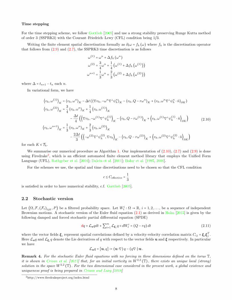
Time stepping
For the time stepping scheme, we follow Gottlieb [2005] and use a strong stability preserving Runge Kutta method
of order 3 (SSPRK3) with the Courant–Friedrich–Lewy (CFL) condition being 1/3.
Writing the finite element spatial discretisation formally as ∂tω = fh (ω) where fh is the discretisation operator
that follows from (2.9) and (2.7), the SSPRK3 time discretisation is as follows
ω(1)= ωn +∆fh (ωn)
ω(2)=
3
4ωn +
1
4(ω(1)
+∆fh (ω(1)))
ωn+1=
1
3ωn +
2
3(ω(2)
+∆fh (ω(2)))
where ∆ = tn+1 − tn each n.
In variational form, we have
⟨vh, ω(1)⟩
K= ⟨vh, ω
n⟩K −∆t (⟨∇vh,−ω
n∇⊥ψnh⟩K − ⟨vh,Q − rωn⟩K + ⟨vh, ω
n∇⊥ψnh ⋅ n⟩∂K)
⟨vh, ω(2)⟩
K=
3
4⟨vh, ω
n⟩K +
1
4⟨vh, ω
(1)⟩K
−∆t
4(⟨∇vh,−ω
(1)∇⊥ψ
(1)h ⟩
K− ⟨vh,Q − rω(1)⟩
K+ ⟨vh, ω
(1)∇⊥ψ
(1)h ⋅ n⟩
∂K)
⟨vh, ωn+1⟩
K=
1
3⟨vh, ω
n⟩K +
2
3⟨vh, ω
(2)⟩K
−2∆t
3(⟨−ω(2)
∇⊥ψ
(2)h ,∇vh⟩
K− ⟨vh,Q − rω(2)⟩
K+ ⟨vh, ω
(2)∇⊥ψ
(2)h ⋅ n⟩
∂K)
(2.10)
for each K ∈ Th.
We summarise our numerical procedure as Algorithm 1. Our implementation of (2.10), (2.7) and (2.9) is done
using Firedrake2, which is an efficient automated finite element method library that employs the Unified Form
Language (UFL), Rathgeber et al. [2016]; Dalcin et al. [2011]; Balay et al. [1997, 2016].
For the schemes we use, the spatial and time discretisations need to be chosen so that the CFL condition
c ≤ Ceffective =1
3
is satisfied in order to have numerical stability, c.f. Gottlieb [2005].
2.2 Stochastic version
Let (Ω,F , (Ft)t≥0 , P ) be a filtered probability space. Let W it ∶ Ω → R, i = 1,2, . . . , be a sequence of independent
Brownian motions. A stochastic version of the Euler fluid equation (2.1) as derived in Holm [2015] is given by the
following damped and forced stochastic partial differential equation (SPDE)
dq +Luqdt +∑m
i=1Lξi
q dW it = (Q − rq)dt (2.11)
where the vector fields ξi represent spatial correlations defined by a velocity-velocity correlation matrix Cij = ξiξTj .
Here Luq and Lξiq denote the Lie derivatives of q with respect to the vector fields u and ξ respectively. In particular
we have
Luq = [u, q] ∶= (u ⋅∇) q − (q∇⋅)u .
Remark 4. For the stochastic Euler fluid equations with no forcing in three dimensions defined on the torus T,
it is shown in Crisan et al. [2017] that, for an initial vorticity in W 2,2 (T) , there exists an unique local (strong)
solution in the space W 2,2 (T) . For the two dimensional case considered in the present work, a global existence and
uniqueness proof is being prepared in Crisan and Lang [2018]
2http://www.firedrakeproject.org/index.html
8
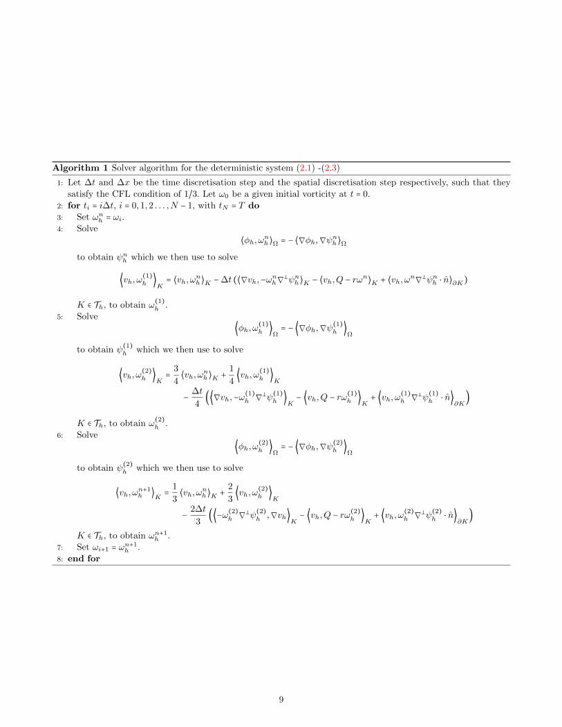
Algorithm 1 Solver algorithm for the deterministic system (2.1) -(2.3)
1: Let ∆t and ∆x be the time discretisation step and the spatial discretisation step respectively, such that they
satisfy the CFL condition of 1/3. Let ω0 be a given initial vorticity at t = 0.
2: for ti = i∆t, i = 0,1,2 . . . ,N − 1, with tN = T do
3: Set ωnh = ωi.
4: Solve
⟨φh, ωnh⟩Ω = − ⟨∇φh,∇ψ
nh⟩Ω
to obtain ψnh which we then use to solve
⟨vh, ω(1)h ⟩
K= ⟨vh, ω
nh⟩K −∆t (⟨∇vh,−ω
nh∇
⊥ψnh⟩K − ⟨vh,Q − rωn⟩K + ⟨vh, ωn∇⊥ψnh ⋅ n⟩∂K)
K ∈ Th, to obtain ω(1)h .
5: Solve
⟨φh, ω(1)h ⟩
Ω= − ⟨∇φh,∇ψ
(1)h ⟩
Ω
to obtain ψ(1)h which we then use to solve
⟨vh, ω(2)h ⟩
K=
3
4⟨vh, ω
nh⟩K +
1
4⟨vh, ω
(1)h ⟩
K
−∆t
4(⟨∇vh,−ω
(1)h ∇
⊥ψ(1)h ⟩
K− ⟨vh,Q − rω
(1)h ⟩
K+ ⟨vh, ω
(1)h ∇
⊥ψ(1)h ⋅ n⟩
∂K)
K ∈ Th, to obtain ω(2)h .
6: Solve
⟨φh, ω(2)h ⟩
Ω= − ⟨∇φh,∇ψ
(2)h ⟩
Ω
to obtain ψ(2)h which we then use to solve
⟨vh, ωn+1h ⟩
K=
1
3⟨vh, ω
nh⟩K +
2
3⟨vh, ω
(2)h ⟩
K
−2∆t
3(⟨−ω
(2)h ∇
⊥ψ(2)h ,∇vh⟩
K− ⟨vh,Q − rω
(2)h ⟩
K+ ⟨vh, ω
(2)h ∇
⊥ψ(2)h ⋅ n⟩
∂K)
K ∈ Th, to obtain ωn+1h .
7: Set ωi+1 = ωn+1h .
8: end for
9
Equation (2.11) arises from the assumption that the Eulerian transport velocity for this flow is described by the
Stratonovich stochastic differential equation (1.2).
Remark 5. One may ask whether the sum in (1.2) should be over an infinite number of terms. For simplification,
we make the assumption that m is finite. This assumption allows us to avoid certain technical issues when we are
interested in the practical aspects for data assimilation.
Assuming u in (1.2) is divergence free, and the ξi are taken to be the eigenvectors of the velocity-velocity
correlation tensor, one can show that ξi are also divergent free vector fields. Hence for each ξi, there exists a
potential function, denoted by ζi, such that
ξi = ∇⊥ζi.
Thus (1.2) can be expressed in terms of ψ and ζi,
dx = ∇⊥ ψdt +∑
m
i=1∇⊥ ζi dW
it . (2.12)
Expressing the transport velocity in this form is useful because it allows us to introduce stochastic perturbation
(i.e. terms with dW it ) via the streamfunction when solving the SPDE system numerically, thereby keeping the
discretisation of (2.11) the same as the deterministic equation (2.1). In other words, upon using the divergence free
properties of u and ξi, we can rewrite (2.11) to obtain
dq +∇⊥ (ψdt +∑m
i=1ζi dW
it ) ⋅ ∇q = (Q − rq)dt , (2.13)
which has the same form as (2.1). Thus, our numerical algorithm for solving the SPDE system is largely the same
as Algorithm 1.
We describe the numerical method in the next subsection and show that it is consistent with the SPDE.
Remark 6. Equation (2.11) is in Stratonovich form. To obtain the equivalent Ito form of (2.11) we apply the
identity
∫
t
0Lξi
q (s) dW is = ∫
t
0Lξi
q (s)dW is +
1
2⟨Lξi
q,W i⟩t
(2.14)
where ⟨., .⟩t is the cross-variation process and
⟨Lξiq,W i⟩
t= Lξi
⟨q,W i⟩t
= Lξi⟨∫ (Q − rq)dt −Luqdt −∑
∞
j=1Lξj
q dW jt ,W
i⟩t
= Lξi⟨−∫
.
0Lξi
q dW is ,W
i⟩t
= Lξi(−∫
t
0Lξi
q (s)ds)
= −∫
t
0L
2ξiq(s)ds
Hence
∫
t
0Lξi
q (s) dW is = ∫
t
0Lξi
q (s)dW is −
1
2∫
t
0L
2ξiq(s)ds
and (2.14) is thus
dq +Luqdt +∑m
i=1Lξi
q dW it =
1
2∑
m
i=1L
2ξiq dt + (Q − rq)dt (2.15)
where L2ξiq = Lξi
(Lξiq) = [ξi, [ξi, q]] is the double Lie derivative of q with respect to the divergence free vector field
ξi.
2.2.1 Numerical implementation
The SPDE system (2.11) has Stratonovich stochastic terms. Consequently, to solve it numerically, the scheme must
take this into account. Of course one could also work with the corresponding Ito form (2.15), in which case the
equation would have a modified drift term.
10
To solve the stochastic system (2.11), we extend the SSPRK3 scheme used in the deterministic case. We will
show that the numerical scheme we introduce is consistent in the sense of Definition 3, see Lang [2010].
Let (Hp, (⋅, ⋅)Hp) be a separable Hilbert space with norm ∥⋅∥Hp
∶=√
(⋅, ⋅)Hp. In our setting, we have Hp =W
p,2,
for some sufficiently large p, see Remark 7. Let Vh be a finite dimensional subspace of Hp. The parameter h ∈ (0,1]
controls the dimension of Vh. For every h, let Ph ∶ Hp → Vh denote the Ritz projection operator mapping elements
of Hp to the finite dimensional subspace Vh such that
limh→0
∥Phq − q∥H = 0
for all q ∈Hp and
(Phq, vh)Hp= (q, vh)Hp
(2.16)
for all q ∈Hp and vh ∈ Vh.
Let f ∶ Hp ×Hp → Hp−1 denote a nonlinear operator which is affine in the second variable, and gi ∶ Hp → Hp−1,
i = 1,2, . . . ,m, are linear mappings from Hp to Hp−1. For notational convenience, we shall write f (⋅) ∶= f (⋅, ⋅) when
the two arguments are the same. Consider the following Stratonovich SPDE
dq(t) = f (q(t))dt +∑m
i=1gi (q(t)) dW i
t . (2.17)
In our model (2.11), f(q) = −Luq + (Q − rq) and gi(q) = −Lξiq. Since u and q satisfy the relation
u = ∇⊥ψ = ∇
⊥∆−1q,
we write f(q).
As noted in Remark 4, for our choice of f and gi, for sufficiently large p the SPDE is well-posed, see Crisan and
Lang [2018]. However, we do not consider the well-posedness of (2.17) for general f and gi, it is beyond the scope
of the present work.
The stochastic SSPRK3 scheme for the SPDE (2.17) is
q(1) = qn + f (qn)∆ +∑m
i=1gi (qn)∆W i
q(2) =3
4qn +
1
4(q(1) + f (q(1))∆ +∑
m
i=1gi (q(1))∆W i)
qn+1=
1
3qn +
2
3(q(2) + f (q(2))∆ +∑
m
i=1gi (q(2))∆W i) , (2.18)
which computes the approximation qn+1 given qn. We will show this time stepping method is consistent in the next
subsection.
We let S∆ ∶Hp ×Ω→Hp−1 denote the one step stochastic SSPRK3 temporal discretisation, that is
qn+1= S∆ (qn) .
The operator S∆ can be seen as the discrete approximation of the solution semigroup operator S (t) ∶Hp ×Ω→Hp
for (2.17). In other words, for an initial condition q0 ∶ Ω→Hp the solution to the SPDE (2.17) is given by
q(t) = S (t) (q0) .
Note that in the continuous case, no differentiability is lost.
Consider the semi-discrete problem on Vh
dqh(t) = fh (qh(t))dt +∑m
i=1gih (qh(t)) dW
it . (2.19)
where fh and gih are spatial approximations to the operators f and gi. In our implementation, like in the PDE case,
we use finite element discretisation to obtain fh and gih. The scheme for the SPDE system is a combination of the
stochastic SSPRK3 scheme for the temporal variable, and a mix of continuous and discontinuous Galerkin finite
11

element approximation for the spatial variables. Algorithm 2 summarises the numerical methodology for the SPDE
system. It is largely the same as Algorithm 1, with the differences (i.e. the additional stochastic terms) highlighted
in red. Note that at each corresponding step in the algorithm, we add the perturbations via the streamfunction,
see (2.13), the result of which is then used to obtain the velocity field u used in the subsequent numerical step.
By substituting q(1)h into q
(2)h , and q
(2)h into qn+1 in (2.18) and expanding fh and gih, the combined spatial and
temporal scheme can be expressed in leading order terms as
qn+1h = S∆ (qnh) = q
nh + fh (qnh)∆ +∑
m
i=1gih (qnh)∆W i
+1
2∑
m
i,j=1gihg
jh (qnh)∆W i∆W j
+H.O.T. (2.20)
where H.O.T. denotes higher order terms.
Algorithm 2 Solver algorithm for the SPDE system
1: Let ∆t and ∆x be the time discretisation step and the spatial discretisation step respectively, such that they
satisfy the CFL condition of 1/3. Let q0 be a given initial vorticity at t = 0.
2: for ti = i∆t, i = 0,1,2 . . . ,N − 1, with tN = T do
3: Set qnh = qi.
4: Let θi ∶= ∑Nj ζj∆W
j for iid ∆W j ∼ N (0,∆t)
5: Solve
⟨φh, qnh⟩Ω = − ⟨∇φh,∇ψ
nh⟩Ω
to obtain ψnh . Let ψnh ∶= ψnh + θi which we then use to solve
⟨vh, q(1)h ⟩
K= ⟨vh, q
nh⟩K −∆t (⟨∇vh,−q
nh∇
⊥ψnh⟩K − ⟨vh,Q − rqn⟩K + ⟨vh, qn∇⊥ψnh ⋅ n⟩∂K)
K ∈ Th, to obtain q(1)h .
6: Solve
⟨φh, q(1)h ⟩
Ω= − ⟨∇φh,∇ψ
(1)h ⟩
Ω
to obtain ψ(1)h . Let ψ
(1)h ∶= ψ
(1)h + θi which we then use to solve
⟨vh, q(2)h ⟩
K=
3
4⟨vh, q
nh⟩K +
1
4⟨vh, q
(1)h ⟩
K
−∆t
4(⟨∇vh,−q
(1)h ∇
⊥ψ(1)h ⟩
K− ⟨vh,Q − rq
(1)h ⟩
K+ ⟨vh, q
(1)h ∇
⊥ψ(1)h ⋅ n⟩
∂K)
K ∈ Th, to obtain q(2)h .
7: Solve
⟨φh, q(2)h ⟩
Ω= − ⟨∇φh,∇ψ
(2)h ⟩
Ω
to obtain ψ(2)h . Let ψ
(2)h ∶= ψ
(2)h + θi which we then use to solve
⟨vh, qn+1h ⟩
K=
1
3⟨vh, q
nh⟩K +
2
3⟨vh, q
(2)h ⟩
K
−2∆t
3(⟨−q
(2)h ∇
⊥ψ(2)h ,∇vh⟩
K− ⟨vh,Q − rq
(2)h ⟩
K+ ⟨vh, q
(2)h ∇
⊥ψ(2)h ⋅ n⟩
∂K)
K ∈ Th, to obtain qn+1h .
8: Set qi+1 = qn+1h .
9: end for
2.2.2 Consistency of the numerical method for the SPDE
We now define consistency for the time stepping scheme for the SPDE (2.17).
12

The approximation operator S∆ can be decomposed into a deterministic part Sd∆ and a stochastic part Ss∆. The
deterministic part correspond to the SSPRK3 discretisation (2.10) for the PDE system (2.1). The stochastic part
Ss∆ should satisfy additional compatibility condition, see Definition 2, in order to be consistent with Stratonovich
integrals.
Definition 1. The local truncation error ej (∆) of the discretisation scheme (2.18) is defined by
ej (∆) = q (tj+1) − S∆q (tj) . (2.21)
The corresponding deterministic local truncation error is
edj (∆) = ω (tj+1) − Sd∆ω (tj) , (2.22)
where ω solves the deterministic system (2.1).
Definition 2. For some γ > 1, the discrete approximation operators Ss∆ is called F-compatible if Ss∆ is Ftj+1measurable and
E (Ss∆ (q (tj))∣Ftj) =1
2∆∑
m
i=1gigiq (tj) +O(∆γ
) (2.23)
for all j = 0, . . . , n − 1.
Definition 3. [Consistency] We say the numerical scheme S∆ is consistent in mean square of order γ > 1 with
respect to (2.17) if there exists a constant c independent of ∆ ∈ (0, T ] and if for all ε > 0, there exist η, δ > 0 such
that for all 0 < ∆ < δ, and j ∈ 1,2, . . . ,N
E (∥ej (∆)∥2H) < c∆γ (2.24)
and
E (∥edj (∆)∥H) < c∆γ (2.25)
and Ss∆ is F-compatible.
Henceforth we introduce a few notational simplifications. Let fs(qt) denote f (qs, qt) when f depends on the
solution at two different times. In our model, this means fs(qt) = −Lusqt + (Q − rqt), and without the subscript we
have f(qt) = −Lutqt + (Q − rqt). Also, since fs(⋅) is affine, we can express it as the summation of a linear part and
a translation, fs(⋅) = As(⋅) +B, where As denotes the linear part, and B denotes the translation.
A 1. We assume the following are bounded,
E (supk ∥fkq (tn) − f (qn)∥2H),
E (sups supr ∥Asfr (qr)∥2H),
E (sups supr ∥Asgigi (qr)∥
2
H),
E (sups supr ∥Asgi (qr)∥
2
H),
E (supr ∥gifr (qr)∥
2
H),
E (supr ∥gigj (qr)∥
2
H),
E (supr ∥gigjgj (qr)∥
2
H).
We also assume that the terms in H.O.T. in (2.20) are bounded in expected H norm squared.
Remark 7. Assumption A1 holds provided the SPDE is well-posed and for all T > 0 and for sufficiently large p,
we have
E⎛
⎝supt∈[0,T ]
∥q(t)∥2p,2
⎞
⎠<∞,
see Crisan and Lang [2018].
13
Lemma 4. Assuming the SPDE (2.17) is well-posed, and Assumption 1 is satisfied, the numerical scheme S∆
described by (2.18) is consistent with γ = 2.
We prove Lemma 4 next. To prove Lemma 4, first note that the mean square of the local truncation error (2.24)
can be bounded as follows.
Lemma 5.
E (∥en (∆)∥2H) ≤ 4E (∥∫
tn+1
tn(f (q(s)) − f (qn))ds∥
2
H)
+ 4E (∥∑m
i=1 ∫
tn+1
tn(gi (qs) − g
i(qn))dW i
s∥
2
H)
+4E (∥1
2∑
m
i=1(∫
tn+1
tngigi (qs)ds −∑
m
j=1gigj (qn)∆W i∆W j
)∥
2
H)
+ 4E (∥H.O.T.∥2H) (2.26)
Proof. Writing the SPDE (2.17) in Ito integral form we have
q (tn+1) = q (tn) + ∫tn+1
tnf (qs)ds +∑
m
i=1 ∫
tn+1
tngi (qs)dW
is +
1
2∑
m
i=1 ∫
tn+1
tngigi (qs)ds (2.27)
Thus, using (2.20) we get
E (∥q (tn+1) − S∆ (qn)∥2H) = E (∥∫
tn+1
tn(f (qs) − f (qn))ds
+∑m
i=1 ∫
tn+1
tn(gi (qs) − g
i(qn))dW i
s
+1
2∑
m
i=1(∫
tn+1
tngigi (qs)ds −∑
m
j=1gigj (qn)∆W i∆W j
)
− H.O.T.∥2H) (2.28)
Using the inequality (x1 + x2 + ⋅ ⋅ ⋅ + xn)2≤ n (x2
1 + x22 + ⋅ ⋅ ⋅ + x
2n), we have the result.
We bound each term in (2.26) individually.
Lemma 6.
E (∥∫
tn+1
tn(f (qs) − f (qn))ds∥
2
H) = O (∆2)
Proof. Using (2.27), we have
f (qs) = fsq(tn) + ∫s
tnAsfr (qr)dr +∑
m
i=1 ∫
s
tnAsg
i(qr)dW
ir +
1
2∑
m
i=1 ∫
s
tnAsg
igi (qr)dr
where As is the linear part of fs. Hence
E (∥∫
tn+1
tn(fs (qs) − f (qn))ds∥
2
H) = E (∥∫
tn+1
tnfsq(tn) − f(q
n)ds + ∫
tn+1
tn∫
s
tnAsfr (qr)drds
+∑m
i=1 ∫
tn+1
tn∫
s
tnAsg
i(qr)dW
irds +
1
2∑
m
i=1 ∫
tn+1
tn∫
s
tnAsg
igi (qr)drds∥2
H) .
Using the Cauchy–Schwarz inequality we have
E (∥∫
tn+1
tnfsq (tn) − f (qn)ds∥
2
H) ≤ ∆∫
tn+1
tnE (∥fsq (tn) − f (qn)∥
2H)ds
≤ E (supk
∥fkq (tn) − f (qn)∥2H)∆2
14

E (∥∫
tn+1
tn∫
s
tnAsfr (qr)drds∥
2
H) ≤ ∆∫
tn+1
tn(s − tn)∫
s
tnE (∥Asfr (qr)∥
2H)drds
≤ E (sups
supr
∥Asfr (qr)∥2H)∆∫
tn+1
tn(s − tn)
2ds
≤ E (sups
supr
∥Asfr (qr)∥2H)
1
3∆4
E (∥1
2∑
m
i=1 ∫
tn+1
tn∫
s
tnAsg
igi (qr)drds∥2
H) ≤
m
4∑
m
i=1∆∫
tn+1
tn(s − tn)∫
s
tnE (∥Asg
igi (qr)∥2
H)drds
≤m2
12E (max
isups
supr
∥Asgigi (qr)∥
2
H)∆4.
Using the Cauchy–Schwarz inequality and Ito isometry we have
E (∥∑m
i=1 ∫
tn+1
tn∫
s
tnAsg
i(qr)dW
irds∥
2
H) ≤m∆∑
m
i=1 ∫
tn+1
tn∫
s
tnE (∥Asg
i(qr)∥
2
H)drds
≤m2
2E (max
isups
supr
∥Asgi(qr)∥
2
H)∆3.
Collect the bounds together to obtain the result.
Lemma 7.
E (∥∑m
i=1 ∫
tn+1
tn(gi (qs) − g
i(qn))dW i
s∥
2
H) = O (∆2)
Proof. Using (2.27), we obtain
gi (qs) = giq(tn) + ∫
s
tngifr (qr)dr +∑
m
j=1 ∫
s
tngigj (qr)dW
jr +
1
2∑
m
j=1 ∫
s
tngigjgj (qr)dr.
Hence
E (∥∑m
i=1 ∫
tn+1
tn(gi (qs) − g
i(qn))dW i
s∥
2
H) = E (∥∑
m
i=1 ∫
tn+1
tn∫
s
tngifr (qr)drdW
is
+∑m
i=1∑m
j=1 ∫
tn+1
tn∫
s
tngigj (qr)dW
jr dW
is
+1
2∑
m
i=1∑m
j=1 ∫
tn+1
tn∫
s
tngigjgj (qr)drdW
is∥
2
H) .
We bound each term individually and obtain the following
E (∥∑m
i=1 ∫
tn+1
tn∫
s
tngifr (qr)drdW
is∥
2
H) ≤m∑
m
i=1 ∫
tn+1
tnE (∥∫
s
tngifr (qr)dr∥
2
H)ds
≤m2
3E (max
isupr
∥gifr (qr)∥2
H)∆3
E (∥∑m
i=1∑m
j=1 ∫
tn+1
tn∫
s
tngigj (qr)dW
jr dW
is∥
2
H) ≤
m4
2E (max
i,jsupr
∥gigj (qr)∥2
H)∆2
E (∥1
2∑
m
i=1∑m
j=1 ∫
tn+1
tn∫
s
tngigjgj (qr)drdW
is∥
2
H) ≤
m4
12E (max
i,jsupr
∥gigjgj (qr)∥2
H)∆3.
Collect the bounds together to obtain the result.
15
Lemma 8.
E (∥1
2∑
m
i=1 ∫
tn+1
tngigi (qs)ds −
1
2∑
m
i=1∑m
j=1gigj (qn)∆W i∆W j
∥
2
H) = O (∆2)
Proof. We have
E (∥1
2∑
m
i=1 ∫
tn+1
tngigi (qs)ds −
1
2∑
m
i=1∑m
j=1gigj (qn)∆W i∆W j
∥
2
H)
≤m
4∑
m
i=1E (∥∫
tn+1
tngigi (qs)ds −∑
m
j=1gigj (qn)∆W i∆W j
∥
2
H)
≤m
4∑
m
i=1E (∥∫
tn+1
tngigi (q(tn))ds −∑
m
j=1gigj (qn)∆W i∆W j
+ ∫
tn+1
tn∫
s
tnH.O.T. ds∥
2
H)
≤m
4∆2∑
m
i=14 [E (∥gigi (q(tn))∥
2
H) +m∑
m
j=1E (∥gigj (qn)∥
2
H)]
+m
4∑
m
i=12E (∥∫
tn+1
tn∫
s
tnH.O.T. ds∥
2
H)
By combining the estimates together we obtain the consistency condition (2.24). For (2.25), the deterministic
part is simply the deterministic SSPRK3 scheme (2.10), see Gottlieb [2005]. The compatibility condition (2.23) for
the stochastic part follows from the leading order term expression (2.20) of the stochastic SSPRK3 scheme and the
fact that
E (∑m
j=1gigj (qn)∆W i∆W j
∣Ftn) = E (gigi (qn)∆W i∆W i∣Ftn) = gigi (qn)∆
as W i and W j are independent for i ≠ j.
3 Calibration of the correlation eigenvectors
3.1 Methodology
In the stochastic geophysical fluid dynamics framework, SPDEs are derived from the starting assumption that
(averaged) fluid particles satisfy the equation
dx(a, t) = u(x(a, t), t)dt +∑m
i=1ξi(x(a, t)) dW
it , (3.1)
where a is the Lagrangian label. The assumption (3.1) leads, for example, to the Eulerian stochastic QG equation,
dq(x, t) + (u(x, t)dt +∑iξi(x, t) dW
it ) ⋅ ∇q(x, t) = 0. (3.2)
Equation (3.2) is what we actually solve. Equation (3.1) is not explicitly solved. However, (3.1) describes the
motion of fluid particles under the SPDE solution, and is used to derive the SPDE.
The goal of the stochastic PDE is to model the coarse-grained components of a deterministic PDE that exhibits
rapidly fluctuating components. We can estimate the components ξi in the stochastic term by comparing (3.1) with
the deterministic equation for unapproximated trajectories,
dx(a, t) = u(x(a, t), t)dt, x(a,0) = xa0 (3.3)
moving with the unapproximated velocity u and starting from xa0 . We assume that the velocity can be written as
u = u+ ζ, where u is a spatially-filtered velocity that can be represented accurately in a coarse-grid simulation. By
comparing (3.1) and (3.3),
dx(a, t) = u(x(a, t), t)dt +∑m
i=1ξi(x(a, t)) dW
it
≈ u(x(a, t), t)dt,
16
where we determine dx(a, t) at the coarse resolution from u(x(a, t), t)dt at the fine resolution, we see that we are
seeking an approximation such that
∑iξi(x(a, t), t) dW
it ≈ u(x(a, t), t)dt − u(x(a, t), t)dt. (3.4)
Our methodology is as follows. We spin up a fine grid simulation from t = −Tspin to t = 0 (till some statistical
equilibrium is reached), then we record velocity time series from t = 0 to t =M∆t, where ∆t = kδt and δt is the fine
grid timestep. We define X0ij as coarse grid points.
For each m = 0,1, . . . ,M − 1, we
1. Solve Xij(t) = u(Xij(t), t) with initial condition Xij(m∆t) =X0ij , where u(x, t) is the solution from the fine
grid simulation.
2. Compute uij(t) by spatially averaging u over the coarse grid box size around gridpoint ij.
3. Compute Xij by solving ˙Xij(t) = uij(t) with the same initial condition.
4. Compute the difference ∆Xmij = Xij((m+1)∆t)−Xij((m+1)∆t), which measures the error between the fine
and coarse trajectory.
Having obtained ∆Xmij , we would like to extract the basis for the noise. This amounts to a Gaussian model of
the form∆Xm
ij√
∆t= ¯∆Xij +∑
N
k=1ξkij∆W
km,
where ∆W km are i.i.d. standard Gaussian random variables.
We estimate ξ by minimising
E⎡⎢⎢⎢⎢⎣
∥∑ijm
∆Xmij
√δt
− ¯∆Xij −∑N
k=1ξkij∆W
km∥
2⎤⎥⎥⎥⎥⎦
,
where the choice of N can be informed by using EOFs.
Remark 8 (EOF). Empirical orthogonal functions (EOFs) can be thought of as principal components that corre-
spond to the spatial correlations of a field, see Hannachi [2004]; Hannachi et al. [2007]. In our case, EOFs are the
eigenvectors of the velocity-velocity spatial covariance tensor. Writing the data time series ∆Xmij , m = 0, . . . ,M − 1
as a matrix F whose entries are two dimensional vectors, and whose rows (row index m) correspond to serialised
∆Xmij . Let F ∶= detrend(F ) where the detrend function removes the column mean from each entry. We then es-
timate the spatial covariance tensor by computing R ∶= 1M−1
FTF . We take the EOFs to be the eigenvectors of R,
ranked in descending order according to the eigenvalues.
3.2 Numerical experiments
3.2.1 Fine grid PDE solution and its coarse graining
We solve the PDE system (2.1)–(2.5) on a fine grid of size 512 × 512. Our choices for α and β in the forcing
term (2.4) are 0.1 and 8, respectively. We apply a coarse-graining procedure to the fine grid solution to obtain
its coarse-grained version on a coarse grid of size 64 × 64, which we call the truth. The coarse-graining procedure
comprises of two steps. First we apply spatial averaging, using for example the Helmholtz operator, to the fine
grid streamfunction. Then this spatially-averaged streamfunction is directly projected onto the coarse grid. The
coarse-grained versions of the vorticity and velocity fields are obtained from the coarse-grained streamfunction.
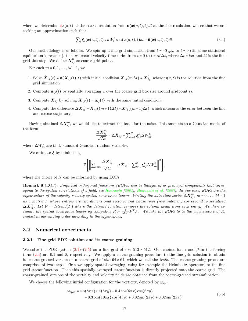
We choose the following initial configuration for the vorticity, denoted by ωspin,
ωspin = sin(8πx) sin(8πy) + 0.4 cos(6πx) cos(6πy)
+ 0.3 cos(10πx) cos(4πy) + 0.02 sin(2πy) + 0.02 sin(2πx)(3.5)
17
from which we spin–up the system until an energy equilibrium state seems to have been reached. This equilibrium
state, denoted by ωinitial, is then chosen as the initial condition for our numerical experiments.
For our numerical experiments, time is measured in terms of large eddy turnover time, henceforth abbreviated
to ett. It describes the time scale of the large scale flow features and is defined by τL = L/U , where L is the length
scale of the largest eddy and U is the mean velocity. Using the numerical PDE solution we estimate that, in our
setup 1 ett is equivalent to 2.5 time units corresponding to the deterministic system.
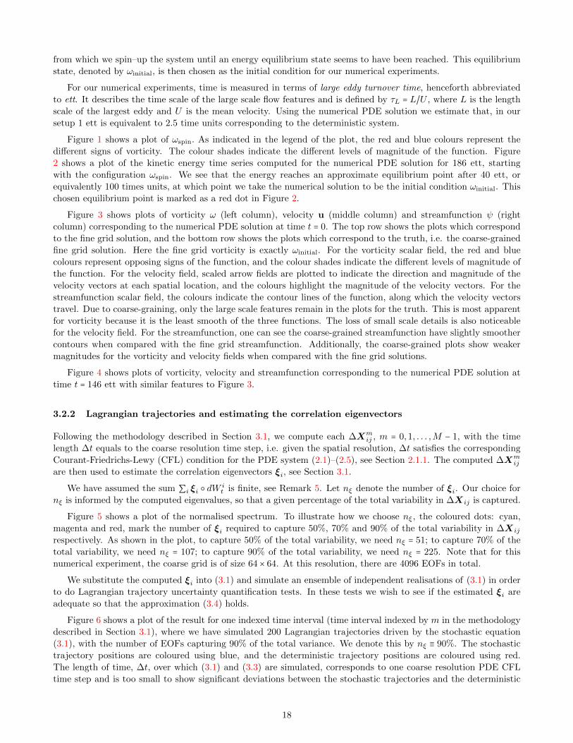
Figure 1 shows a plot of ωspin. As indicated in the legend of the plot, the red and blue colours represent the
different signs of vorticity. The colour shades indicate the different levels of magnitude of the function. Figure
2 shows a plot of the kinetic energy time series computed for the numerical PDE solution for 186 ett, starting
with the configuration ωspin. We see that the energy reaches an approximate equilibrium point after 40 ett, or
equivalently 100 times units, at which point we take the numerical solution to be the initial condition ωinitial. This
chosen equilibrium point is marked as a red dot in Figure 2.
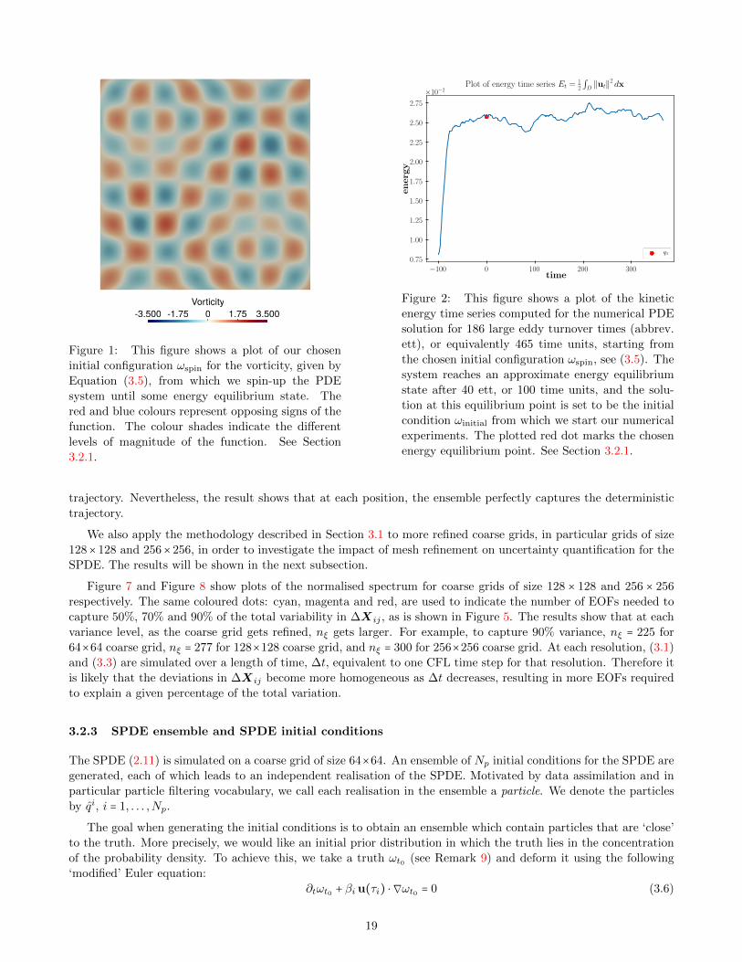
Figure 3 shows plots of vorticity ω (left column), velocity u (middle column) and streamfunction ψ (right
column) corresponding to the numerical PDE solution at time t = 0. The top row shows the plots which correspond
to the fine grid solution, and the bottom row shows the plots which correspond to the truth, i.e. the coarse-grained
fine grid solution. Here the fine grid vorticity is exactly ωinitial. For the vorticity scalar field, the red and blue
colours represent opposing signs of the function, and the colour shades indicate the different levels of magnitude of
the function. For the velocity field, scaled arrow fields are plotted to indicate the direction and magnitude of the
velocity vectors at each spatial location, and the colours highlight the magnitude of the velocity vectors. For the
streamfunction scalar field, the colours indicate the contour lines of the function, along which the velocity vectors
travel. Due to coarse-graining, only the large scale features remain in the plots for the truth. This is most apparent
for vorticity because it is the least smooth of the three functions. The loss of small scale details is also noticeable
for the velocity field. For the streamfunction, one can see the coarse-grained streamfunction have slightly smoother
contours when compared with the fine grid streamfunction. Additionally, the coarse-grained plots show weaker
magnitudes for the vorticity and velocity fields when compared with the fine grid solutions.
Figure 4 shows plots of vorticity, velocity and streamfunction corresponding to the numerical PDE solution at
time t = 146 ett with similar features to Figure 3.
3.2.2 Lagrangian trajectories and estimating the correlation eigenvectors
Following the methodology described in Section 3.1, we compute each ∆Xmij , m = 0,1, . . . ,M − 1, with the time
length ∆t equals to the coarse resolution time step, i.e. given the spatial resolution, ∆t satisfies the corresponding
Courant-Friedrichs-Lewy (CFL) condition for the PDE system (2.1)–(2.5), see Section 2.1.1. The computed ∆Xmij
are then used to estimate the correlation eigenvectors ξi, see Section 3.1.
We have assumed the sum ∑i ξi dWit is finite, see Remark 5. Let nξ denote the number of ξi. Our choice for
nξ is informed by the computed eigenvalues, so that a given percentage of the total variability in ∆Xij is captured.
Figure 5 shows a plot of the normalised spectrum. To illustrate how we choose nξ, the coloured dots: cyan,
magenta and red, mark the number of ξi required to capture 50%, 70% and 90% of the total variability in ∆Xij
respectively. As shown in the plot, to capture 50% of the total variability, we need nξ = 51; to capture 70% of the
total variability, we need nξ = 107; to capture 90% of the total variability, we need nξ = 225. Note that for this
numerical experiment, the coarse grid is of size 64 × 64. At this resolution, there are 4096 EOFs in total.
We substitute the computed ξi into (3.1) and simulate an ensemble of independent realisations of (3.1) in order
to do Lagrangian trajectory uncertainty quantification tests. In these tests we wish to see if the estimated ξi are
adequate so that the approximation (3.4) holds.
Figure 6 shows a plot of the result for one indexed time interval (time interval indexed by m in the methodology
described in Section 3.1), where we have simulated 200 Lagrangian trajectories driven by the stochastic equation
(3.1), with the number of EOFs capturing 90% of the total variance. We denote this by nξ ≡ 90%. The stochastic
trajectory positions are coloured using blue, and the deterministic trajectory positions are coloured using red.
The length of time, ∆t, over which (3.1) and (3.3) are simulated, corresponds to one coarse resolution PDE CFL
time step and is too small to show significant deviations between the stochastic trajectories and the deterministic
18
-1.75 0 1.75-3.500 3.500Vorticity
Figure 1: This figure shows a plot of our chosen
initial configuration ωspin for the vorticity, given by
Equation (3.5), from which we spin-up the PDE
system until some energy equilibrium state. The
red and blue colours represent opposing signs of the
function. The colour shades indicate the different
levels of magnitude of the function. See Section
3.2.1.
Figure 2: This figure shows a plot of the kinetic
energy time series computed for the numerical PDE
solution for 186 large eddy turnover times (abbrev.
ett), or equivalently 465 time units, starting from
the chosen initial configuration ωspin, see (3.5). The
system reaches an approximate energy equilibrium
state after 40 ett, or 100 time units, and the solu-
tion at this equilibrium point is set to be the initial
condition ωinitial from which we start our numerical
experiments. The plotted red dot marks the chosen
energy equilibrium point. See Section 3.2.1.
trajectory. Nevertheless, the result shows that at each position, the ensemble perfectly captures the deterministic
trajectory.
We also apply the methodology described in Section 3.1 to more refined coarse grids, in particular grids of size
128× 128 and 256× 256, in order to investigate the impact of mesh refinement on uncertainty quantification for the
SPDE. The results will be shown in the next subsection.
Figure 7 and Figure 8 show plots of the normalised spectrum for coarse grids of size 128 × 128 and 256 × 256
respectively. The same coloured dots: cyan, magenta and red, are used to indicate the number of EOFs needed to
capture 50%, 70% and 90% of the total variability in ∆Xij , as is shown in Figure 5. The results show that at each
variance level, as the coarse grid gets refined, nξ gets larger. For example, to capture 90% variance, nξ = 225 for
64×64 coarse grid, nξ = 277 for 128×128 coarse grid, and nξ = 300 for 256×256 coarse grid. At each resolution, (3.1)
and (3.3) are simulated over a length of time, ∆t, equivalent to one CFL time step for that resolution. Therefore it
is likely that the deviations in ∆Xij become more homogeneous as ∆t decreases, resulting in more EOFs required
to explain a given percentage of the total variation.
3.2.3 SPDE ensemble and SPDE initial conditions
The SPDE (2.11) is simulated on a coarse grid of size 64×64. An ensemble of Np initial conditions for the SPDE are
generated, each of which leads to an independent realisation of the SPDE. Motivated by data assimilation and in
particular particle filtering vocabulary, we call each realisation in the ensemble a particle. We denote the particles
by qi, i = 1, . . . ,Np.
The goal when generating the initial conditions is to obtain an ensemble which contain particles that are ‘close’
to the truth. More precisely, we would like an initial prior distribution in which the truth lies in the concentration
of the probability density. To achieve this, we take a truth ωt0 (see Remark 9) and deform it using the following
‘modified’ Euler equation:
∂tωt0 + βi u(τi) ⋅ ∇ωt0 = 0 (3.6)
19
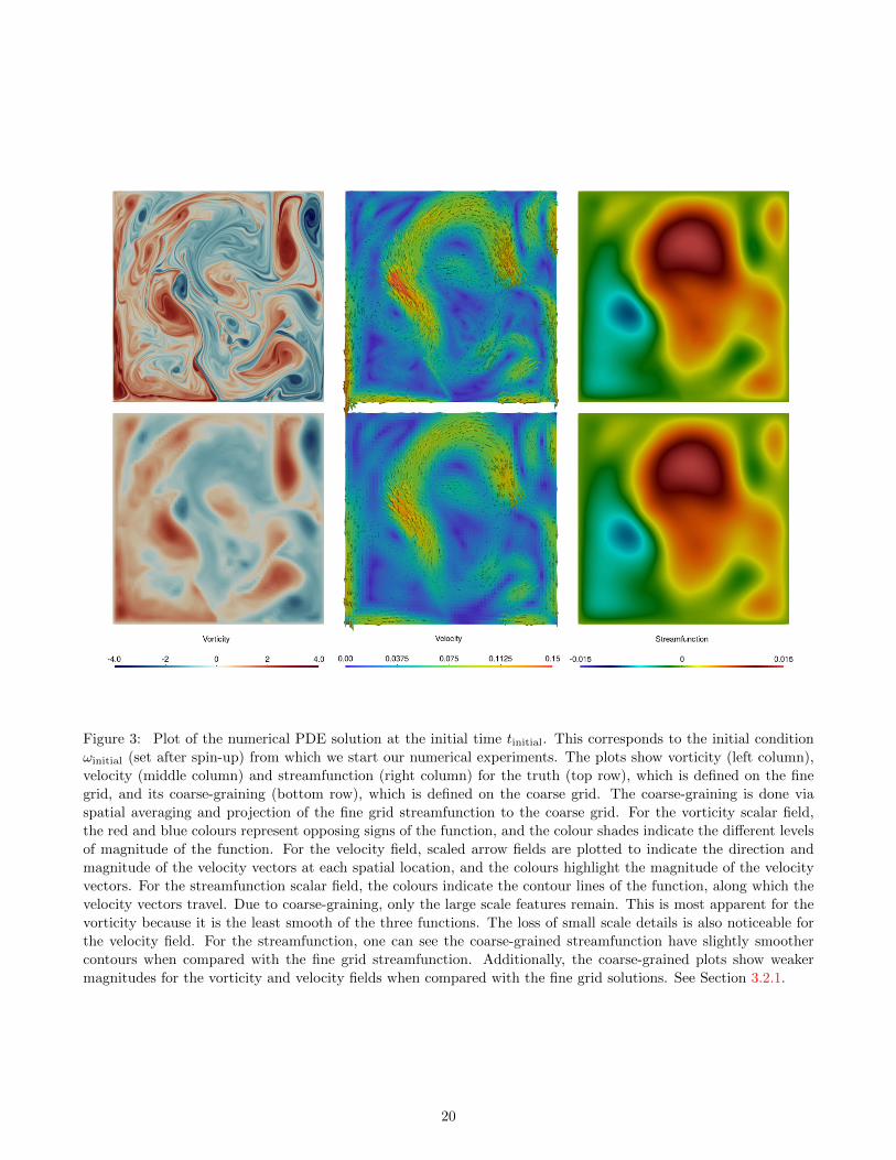
Figure 3: Plot of the numerical PDE solution at the initial time tinitial. This corresponds to the initial condition
ωinitial (set after spin-up) from which we start our numerical experiments. The plots show vorticity (left column),
velocity (middle column) and streamfunction (right column) for the truth (top row), which is defined on the fine
grid, and its coarse-graining (bottom row), which is defined on the coarse grid. The coarse-graining is done via
spatial averaging and projection of the fine grid streamfunction to the coarse grid. For the vorticity scalar field,
the red and blue colours represent opposing signs of the function, and the colour shades indicate the different levels
of magnitude of the function. For the velocity field, scaled arrow fields are plotted to indicate the direction and
magnitude of the velocity vectors at each spatial location, and the colours highlight the magnitude of the velocity
vectors. For the streamfunction scalar field, the colours indicate the contour lines of the function, along which the
velocity vectors travel. Due to coarse-graining, only the large scale features remain. This is most apparent for the
vorticity because it is the least smooth of the three functions. The loss of small scale details is also noticeable for
the velocity field. For the streamfunction, one can see the coarse-grained streamfunction have slightly smoother
contours when compared with the fine grid streamfunction. Additionally, the coarse-grained plots show weaker
magnitudes for the vorticity and velocity fields when compared with the fine grid solutions. See Section 3.2.1.
20
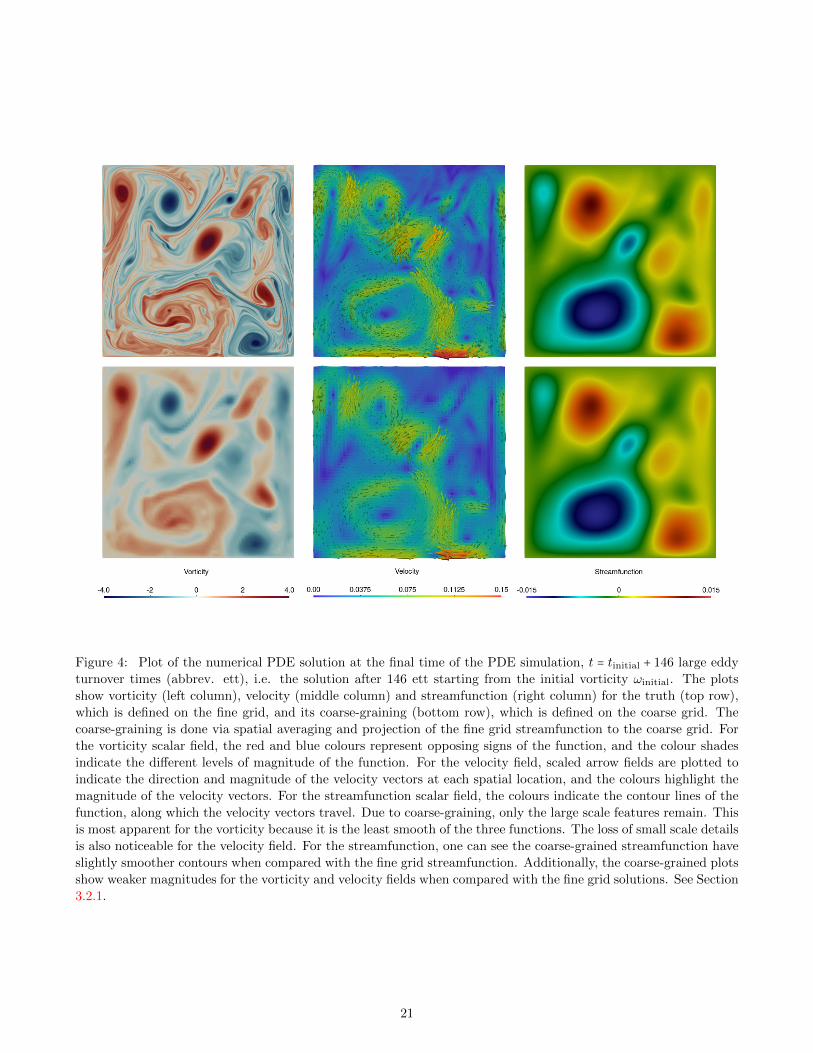
Figure 4: Plot of the numerical PDE solution at the final time of the PDE simulation, t = tinitial + 146 large eddy
turnover times (abbrev. ett), i.e. the solution after 146 ett starting from the initial vorticity ωinitial. The plots
show vorticity (left column), velocity (middle column) and streamfunction (right column) for the truth (top row),
which is defined on the fine grid, and its coarse-graining (bottom row), which is defined on the coarse grid. The
coarse-graining is done via spatial averaging and projection of the fine grid streamfunction to the coarse grid. For
the vorticity scalar field, the red and blue colours represent opposing signs of the function, and the colour shades
indicate the different levels of magnitude of the function. For the velocity field, scaled arrow fields are plotted to
indicate the direction and magnitude of the velocity vectors at each spatial location, and the colours highlight the
magnitude of the velocity vectors. For the streamfunction scalar field, the colours indicate the contour lines of the
function, along which the velocity vectors travel. Due to coarse-graining, only the large scale features remain. This
is most apparent for the vorticity because it is the least smooth of the three functions. The loss of small scale details
is also noticeable for the velocity field. For the streamfunction, one can see the coarse-grained streamfunction have
slightly smoother contours when compared with the fine grid streamfunction. Additionally, the coarse-grained plots
show weaker magnitudes for the vorticity and velocity fields when compared with the fine grid solutions. See Section
3.2.1.
21

Figure 5: EOF normalised spectrum for coarse grid size
64 × 64. To illustrate how we choose nξ, the coloured
dots: cyan, magenta and red, mark the number of ξirequired to capture 50%, 70% and 90% of the total vari-
ability in ∆Xij respectively. As shown in the plot, to
capture 50% of the total variability, we need nξ = 51; to
capture 70% of the total variability, we need nξ = 107; to
capture 90% of the total variability, we need nξ = 225.
Note that at this resolution, there are 4096 EOFs in
total. See Section 3.2.2.
Figure 6: Lagrangian trajectory uncertainty quantifica-
tion corresponding to the time interval [50,52) in simu-
lation time units, see Section 3.1. There are 200 stochas-
tic Lagrangian trajectories (driven by the stochastic
equation (3.1)), using a number of EOFs capturing 90%
of the total variance, nξ ≡ 90%. The length of time, ∆t,
over which (3.1) and (3.3) are simulated, corresponds to
one coarse resolution PDE CFL time step. The stochas-
tic trajectory positions are coloured using blue, and
the deterministic trajectory positions are coloured using
red. The time step ∆t is too small to show significant
deviations between the stochastic trajectories and the
deterministic trajectory. Nevertheless, the plot shows
that at each position, the ensemble perfectly captures
the deterministic trajectory. See Section 3.2.2.
where βi ∼ N (0, ε), i = 1, . . . ,Np are centered Gaussian weights with an apriori variance parameter ε, and τi ∼
U (tinitial, t0) , i = 1, . . . ,Np are uniform random numbers. Thus each u (τi) corresponds to a PDE solution in the
time period [tinitial, t0). Equation (3.6) is solved for one or two ett to obtain a deformation ωit0 of the coarse grained
initial condition ωt0 . These are then used as initial conditions for the SPDE realisations, i.e. qit0 ∶= ωit0 , i = 1, . . . ,Np.
Remark 9. At the start of Section 3.2 we discussed simulating the PDE on the fine grid. The PDE initial condition
ωinitial was obtained after spin–up. The overall simulation time interval from the point of ωinitial is of length 146
ett. Let tinitial denote the time point that corresponds to ωinitial. We divide the overall simulation time interval into
two halves [tinitial, t0) and [t0,146] . The PDE solutions in the period [tinitial, t0) are used for generating the initial
condition ensemble for the SPDE, see (3.6). This way, the velocity field used in (3.6) is physical. t0 is set as the
initial time to start the SPDE uncertainty quantification numerical experiments.
Figures 9, 10 and 11 show plots for the truth and two independent realisations of the SPDE at times t0, t0 + 3
ett and t0 + 5 ett, respectively. In each figure, the plots show vorticity (left column), velocity (middle column) and
streamfunction (right column) for the truth (top row), and the two particles (middle and bottom rows).
In Figure 9 the particles are generated using the deformation procedure (3.6). Intuitively, deformations of the
truth hope to capture the idea of “location uncertainty” in the initial conditions. The middle particle seems to be
‘closer’ to the truth in terms of the visible large scale features than the bottom particle.
At time t0 + 3 ett, which is shown in Figure 10, although the middle particle started ‘closer’ to the truth than
the bottom particle at time t0, different large and small scale features to the truth have developed. Comparing
the streamfunction plots, the bottom particle seems to have diverged from the truth even further. Seen at t0 + 5
22
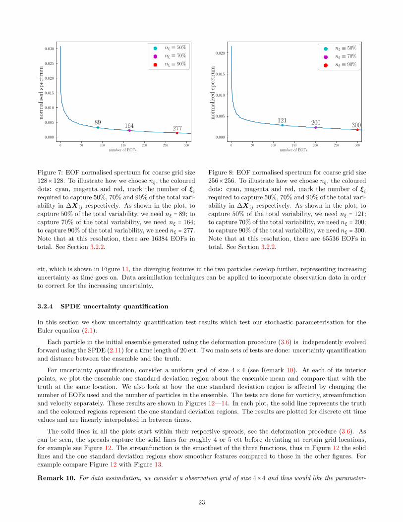
Figure 7: EOF normalised spectrum for coarse grid size
128× 128. To illustrate how we choose nξ, the coloured
dots: cyan, magenta and red, mark the number of ξirequired to capture 50%, 70% and 90% of the total vari-
ability in ∆Xij respectively. As shown in the plot, to
capture 50% of the total variability, we need nξ = 89; to
capture 70% of the total variability, we need nξ = 164;
to capture 90% of the total variability, we need nξ = 277.
Note that at this resolution, there are 16384 EOFs in
total. See Section 3.2.2.
Figure 8: EOF normalised spectrum for coarse grid size
256× 256. To illustrate how we choose nξ, the coloured
dots: cyan, magenta and red, mark the number of ξirequired to capture 50%, 70% and 90% of the total vari-
ability in ∆Xij respectively. As shown in the plot, to
capture 50% of the total variability, we need nξ = 121;
to capture 70% of the total variability, we need nξ = 200;
to capture 90% of the total variability, we need nξ = 300.
Note that at this resolution, there are 65536 EOFs in
total. See Section 3.2.2.
ett, which is shown in Figure 11, the diverging features in the two particles develop further, representing increasing
uncertainty as time goes on. Data assimilation techniques can be applied to incorporate observation data in order
to correct for the increasing uncertainty.
3.2.4 SPDE uncertainty quantification
In this section we show uncertainty quantification test results which test our stochastic parameterisation for the
Euler equation (2.1).
Each particle in the initial ensemble generated using the deformation procedure (3.6) is independently evolved
forward using the SPDE (2.11) for a time length of 20 ett. Two main sets of tests are done: uncertainty quantification
and distance between the ensemble and the truth.
For uncertainty quantification, consider a uniform grid of size 4 × 4 (see Remark 10). At each of its interior
points, we plot the ensemble one standard deviation region about the ensemble mean and compare that with the
truth at the same location. We also look at how the one standard deviation region is affected by changing the
number of EOFs used and the number of particles in the ensemble. The tests are done for vorticity, streamfunction
and velocity separately. These results are shown in Figures 12—14. In each plot, the solid line represents the truth
and the coloured regions represent the one standard deviation regions. The results are plotted for discrete ett time
values and are linearly interpolated in between times.
The solid lines in all the plots start within their respective spreads, see the deformation procedure (3.6). As
can be seen, the spreads capture the solid lines for roughly 4 or 5 ett before deviating at certain grid locations,
for example see Figure 12. The streamfunction is the smoothest of the three functions, thus in Figure 12 the solid
lines and the one standard deviation regions show smoother features compared to those in the other figures. For
example compare Figure 12 with Figure 13.
Remark 10. For data assimilation, we consider a observation grid of size 4×4 and thus would like the parameter-
23

Figure 9: The plots show vorticity (left column), velocity (middle column) and streamfunction (right column) for
the coarse-grained fine solution (top row), which we call the truth, and two independent realisations of the SPDE
(middle and bottom rows) at time t0, which we call particles. The particles at this time point are generated using
the deformation procedure (3.6). For the vorticity scalar field, the red and blue colours represent opposing signs
of the function, and the colour shades indicate the different levels of magnitude of the function. For the velocity
field, scaled arrow fields are plotted to indicate the direction and magnitude of the velocity vectors at each spatial
location, and the colours highlight the magnitude of the velocity vectors. For the streamfunction scalar field, the
colours indicate the contour lines of the function, along which the velocity vectors travel. The middle particle seems
to be ‘closer’ to the truth in terms of the visible large scale features than the bottom particle, see (3.6). See Section
3.2.3.
24

Figure 10: Following on from Figure 9, the plots show vorticity (left column), velocity (middle column) and
streamfunction (right column) for the truth (top row), and the two particles (middle and bottom rows) at time
t0 + 3 ett. For the vorticity scalar field, the red and blue colours represent opposing signs of the function, and
the colour shades indicate the different levels of magnitude of the function. For the velocity field, scaled arrow
fields are plotted to indicate the direction and magnitude of the velocity vectors at each spatial location, and the
colours highlight the magnitude of the velocity vectors. For the streamfunction scalar field, the colours indicate the
contour lines of the function, along which the velocity vectors travel. The middle particle started ‘closer’ to the
truth in terms of the visible large scale features at time t0 than the bottom particle, see Figure 9, however as can
be seen, different large and small scale features to the truth have developed. Comparing the streamfunction plots,
the bottom particle seems to have diverged from the truth even further. See Section 3.2.3.
25

Figure 11: Following on from Figure 10, the plots show vorticity (left column), velocity (middle column) and
streamfunction (right column) for the truth (top row), and the two particles (middle and bottom rows) at time
t0 + 5 ett. For the vorticity scalar field, the red and blue colours represent opposing signs of the function, and
the colour shades indicate the different levels of magnitude of the function. For the velocity field, scaled arrow
fields are plotted to indicate the direction and magnitude of the velocity vectors at each spatial location, and the
colours highlight the magnitude of the velocity vectors. For the streamfunction scalar field, the colours indicate the
contour lines of the function, along which the velocity vectors travel. The middle particle started ‘closer’ to the
truth in terms of the visible large scale features at time t0 than the bottom particle, see Figure 9, however as can
be seen, different large and small scale features to the truth have developed. Comparing the streamfunction plots,
the bottom particle seems to have diverged from the truth even further. See Section 3.2.3.
26
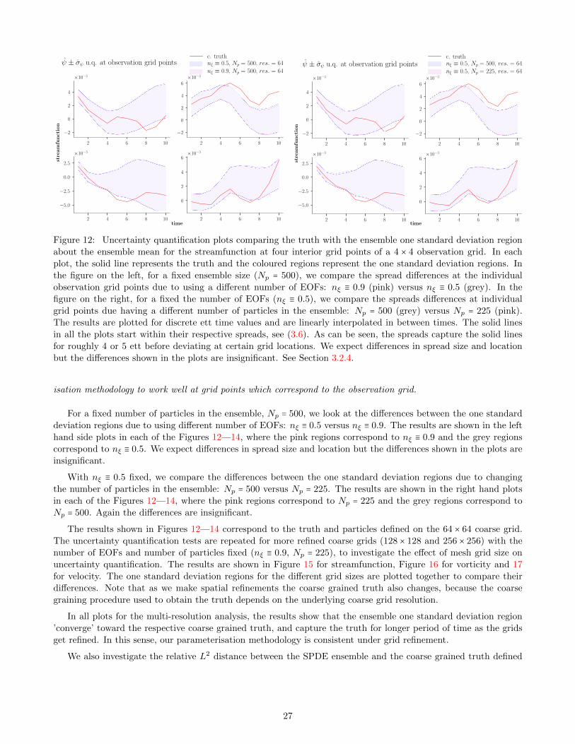
Figure 12: Uncertainty quantification plots comparing the truth with the ensemble one standard deviation region
about the ensemble mean for the streamfunction at four interior grid points of a 4 × 4 observation grid. In each
plot, the solid line represents the truth and the coloured regions represent the one standard deviation regions. In
the figure on the left, for a fixed ensemble size (Np = 500), we compare the spread differences at the individual
observation grid points due to using a different number of EOFs: nξ ≡ 0.9 (pink) versus nξ ≡ 0.5 (grey). In the
figure on the right, for a fixed the number of EOFs (nξ ≡ 0.5), we compare the spreads differences at individual
grid points due having a different number of particles in the ensemble: Np = 500 (grey) versus Np = 225 (pink).
The results are plotted for discrete ett time values and are linearly interpolated in between times. The solid lines
in all the plots start within their respective spreads, see (3.6). As can be seen, the spreads capture the solid lines
for roughly 4 or 5 ett before deviating at certain grid locations. We expect differences in spread size and location
but the differences shown in the plots are insignificant. See Section 3.2.4.
isation methodology to work well at grid points which correspond to the observation grid.
For a fixed number of particles in the ensemble, Np = 500, we look at the differences between the one standard
deviation regions due to using different number of EOFs: nξ ≡ 0.5 versus nξ ≡ 0.9. The results are shown in the left
hand side plots in each of the Figures 12—14, where the pink regions correspond to nξ ≡ 0.9 and the grey regions
correspond to nξ ≡ 0.5. We expect differences in spread size and location but the differences shown in the plots are
insignificant.
With nξ ≡ 0.5 fixed, we compare the differences between the one standard deviation regions due to changing
the number of particles in the ensemble: Np = 500 versus Np = 225. The results are shown in the right hand plots
in each of the Figures 12—14, where the pink regions correspond to Np = 225 and the grey regions correspond to
Np = 500. Again the differences are insignificant.
The results shown in Figures 12—14 correspond to the truth and particles defined on the 64 × 64 coarse grid.
The uncertainty quantification tests are repeated for more refined coarse grids (128 × 128 and 256 × 256) with the
number of EOFs and number of particles fixed (nξ ≡ 0.9, Np = 225), to investigate the effect of mesh grid size on
uncertainty quantification. The results are shown in Figure 15 for streamfunction, Figure 16 for vorticity and 17
for velocity. The one standard deviation regions for the different grid sizes are plotted together to compare their
differences. Note that as we make spatial refinements the coarse grained truth also changes, because the coarse
graining procedure used to obtain the truth depends on the underlying coarse grid resolution.
In all plots for the multi-resolution analysis, the results show that the ensemble one standard deviation region
’converge’ toward the respective coarse grained truth, and capture the truth for longer period of time as the grids
get refined. In this sense, our parameterisation methodology is consistent under grid refinement.
We also investigate the relative L2 distance between the SPDE ensemble and the coarse grained truth defined
27
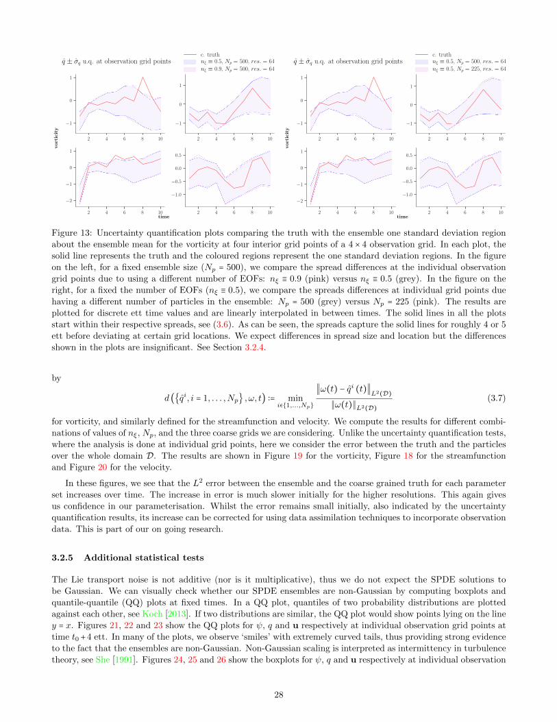
Figure 13: Uncertainty quantification plots comparing the truth with the ensemble one standard deviation region
about the ensemble mean for the vorticity at four interior grid points of a 4 × 4 observation grid. In each plot, the
solid line represents the truth and the coloured regions represent the one standard deviation regions. In the figure
on the left, for a fixed ensemble size (Np = 500), we compare the spread differences at the individual observation
grid points due to using a different number of EOFs: nξ ≡ 0.9 (pink) versus nξ ≡ 0.5 (grey). In the figure on the
right, for a fixed the number of EOFs (nξ ≡ 0.5), we compare the spreads differences at individual grid points due
having a different number of particles in the ensemble: Np = 500 (grey) versus Np = 225 (pink). The results are
plotted for discrete ett time values and are linearly interpolated in between times. The solid lines in all the plots
start within their respective spreads, see (3.6). As can be seen, the spreads capture the solid lines for roughly 4 or 5
ett before deviating at certain grid locations. We expect differences in spread size and location but the differences
shown in the plots are insignificant. See Section 3.2.4.
by
d (qi, i = 1, . . . ,Np , ω, t) ∶= mini∈1,...,Np
∥ω(t) − qi (t)∥L2
(D)
∥ω(t)∥L2(D)
(3.7)
for vorticity, and similarly defined for the streamfunction and velocity. We compute the results for different combi-
nations of values of nξ, Np, and the three coarse grids we are considering. Unlike the uncertainty quantification tests,
where the analysis is done at individual grid points, here we consider the error between the truth and the particles
over the whole domain D. The results are shown in Figure 19 for the vorticity, Figure 18 for the streamfunction
and Figure 20 for the velocity.
In these figures, we see that the L2 error between the ensemble and the coarse grained truth for each parameter
set increases over time. The increase in error is much slower initially for the higher resolutions. This again gives
us confidence in our parameterisation. Whilst the error remains small initially, also indicated by the uncertainty
quantification results, its increase can be corrected for using data assimilation techniques to incorporate observation
data. This is part of our on going research.
3.2.5 Additional statistical tests
The Lie transport noise is not additive (nor is it multiplicative), thus we do not expect the SPDE solutions to
be Gaussian. We can visually check whether our SPDE ensembles are non-Gaussian by computing boxplots and
quantile-quantile (QQ) plots at fixed times. In a QQ plot, quantiles of two probability distributions are plotted
against each other, see Koch [2013]. If two distributions are similar, the QQ plot would show points lying on the line
y = x. Figures 21, 22 and 23 show the QQ plots for ψ, q and u respectively at individual observation grid points at
time t0+4 ett. In many of the plots, we observe ‘smiles’ with extremely curved tails, thus providing strong evidence
to the fact that the ensembles are non-Gaussian. Non-Gaussian scaling is interpreted as intermittency in turbulence
theory, see She [1991]. Figures 24, 25 and 26 show the boxplots for ψ, q and u respectively at individual observation
28
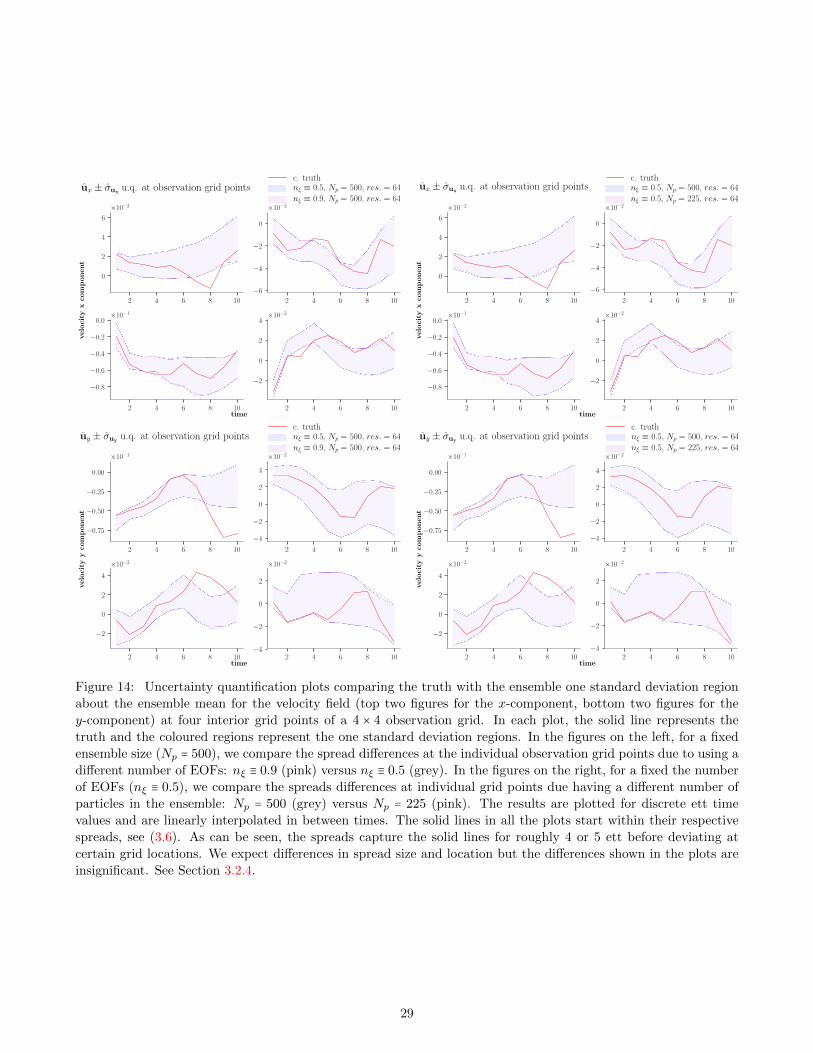
Figure 14: Uncertainty quantification plots comparing the truth with the ensemble one standard deviation region
about the ensemble mean for the velocity field (top two figures for the x-component, bottom two figures for the
y-component) at four interior grid points of a 4 × 4 observation grid. In each plot, the solid line represents the
truth and the coloured regions represent the one standard deviation regions. In the figures on the left, for a fixed
ensemble size (Np = 500), we compare the spread differences at the individual observation grid points due to using a
different number of EOFs: nξ ≡ 0.9 (pink) versus nξ ≡ 0.5 (grey). In the figures on the right, for a fixed the number
of EOFs (nξ ≡ 0.5), we compare the spreads differences at individual grid points due having a different number of
particles in the ensemble: Np = 500 (grey) versus Np = 225 (pink). The results are plotted for discrete ett time
values and are linearly interpolated in between times. The solid lines in all the plots start within their respective
spreads, see (3.6). As can be seen, the spreads capture the solid lines for roughly 4 or 5 ett before deviating at
certain grid locations. We expect differences in spread size and location but the differences shown in the plots are
insignificant. See Section 3.2.4.
29

Figure 15: Uncertainty quantification comparing the truth with the ensemble one standard deviation region about
the ensemble mean for the streamfunction. The left and right hand figures each contain four plots. Each plot
corresponds to a fixed grid point on a observation grid of size 4×4. For a fixed number of EOFs nξ ≡ 0.9 and a fixed
number of particles in the ensemble Np = 225, each plot shows the truths and spreads corresponding to three coarse
resolutions: 64× 64, 128× 128 and 256× 256.. The solid lines represent the truth and the coloured regions represent
the one standard deviation regions. Recall that the truth depends on the coarse grid size, see Figure 3. The red
line and spread correspond to the 64× 64 coarse grid. The green line and spread correspond to the 128× 128 coarse
grid. The blue line and spread correspond to the 256× 256 coarse grid. The results are plotted for discrete ett time
values and are linearly interpolated in between times. We see that as the coarse grid resolution gets refined, the one
standard deviation region stays closer to the truth for longer time periods. This confirms that the parameterisation
methodology is consistent under grid refinement. See Section 3.1 and 3.2.4
.
30
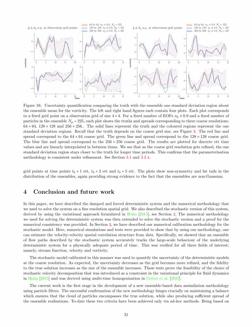
Figure 16: Uncertainty quantification comparing the truth with the ensemble one standard deviation region about
the ensemble mean for the vorticity. The left and right hand figures each contain four plots. Each plot corresponds
to a fixed grid point on a observation grid of size 4× 4. For a fixed number of EOFs nξ ≡ 0.9 and a fixed number of
particles in the ensemble Np = 225, each plot shows the truths and spreads corresponding to three coarse resolutions:
64 × 64, 128 × 128 and 256 × 256.. The solid lines represent the truth and the coloured regions represent the one
standard deviation regions. Recall that the truth depends on the coarse grid size, see Figure 3. The red line and
spread correspond to the 64 × 64 coarse grid. The green line and spread correspond to the 128 × 128 coarse grid.
The blue line and spread correspond to the 256 × 256 coarse grid. The results are plotted for discrete ett time
values and are linearly interpolated in between times. We see that as the coarse grid resolution gets refined, the one
standard deviation region stays closer to the truth for longer time periods. This confirms that the parameterisation
methodology is consistent under refinement. See Section 3.1 and 3.2.4.
grid points at time points t0 + 1 ett, t0 + 2 ett and t0 + 5 ett. The plots show non-symmetry and fat tails in the
distribution of the ensembles, again providing strong evidence to the fact that the ensembles are non-Gaussian.
4 Conclusion and future work
In this paper, we have described the damped and forced deterministic system and the numerical methodology that
we used to solve the system on a fine resolution spatial grid. We also described the stochastic version of this system,
derived by using the variational approach formulated in Holm [2015], see Section 2, The numerical methodology
we used for solving the deterministic system was then extended to solve the stochastic version and a proof for the
numerical consistency was provided. In Section 3, we have described our numerical calibration methodology for the
stochastic model. Here, numerical simulations and tests were provided to show that by using our methodology, one
can estimate the velocity-velocity spatial correlation structure from data. Specifically, we showed that an ensemble
of flow paths described by the stochastic system accurately tracks the large-scale behaviour of the underlying
deterministic system for a physically adequate period of time. This was verified for all three fields of interest;
namely, stream function, velocity and vorticity.
The stochastic model calibrated in this manner was used to quantify the uncertainty of the deterministic models
at the coarse resolution. As expected, the uncertainty decreases as the grid becomes more refined, and the fidelity
to the true solution increases as the size of the ensemble increases. These tests prove the feasibility of the choice of
stochastic velocity decomposition that was introduced as a constraint in the variational principle for fluid dynamics
in Holm [2015] and was derived using multi-time homogenisation in Cotter et al. [2017].
The current work is the first stage in the development of a new ensemble-based data assimilation methodology
using particle filters. The successful confirmation of the new methodology hinges crucially on maintaining a balance
which ensures that the cloud of particles encompasses the true solution, while also producing sufficient spread of
the ensemble realisations. To-date these two criteria have been achieved only via ad-hoc methods. Being based on
31
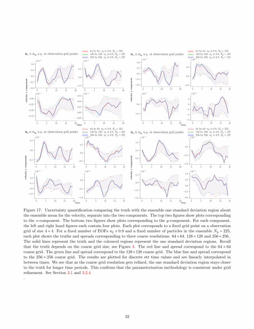
Figure 17: Uncertainty quantification comparing the truth with the ensemble one standard deviation region about
the ensemble mean for the velocity, separate into the two components. The top two figures show plots corresponding
to the x-component. The bottom two figures show plots corresponding to the y-component. For each component,
the left and right hand figures each contain four plots. Each plot corresponds to a fixed grid point on a observation
grid of size 4 × 4. For a fixed number of EOFs nξ ≡ 0.9 and a fixed number of particles in the ensemble Np = 225,
each plot shows the truths and spreads corresponding to three coarse resolutions: 64× 64, 128× 128 and 256× 256..
The solid lines represent the truth and the coloured regions represent the one standard deviation regions. Recall
that the truth depends on the coarse grid size, see Figure 3. The red line and spread correspond to the 64 × 64
coarse grid. The green line and spread correspond to the 128×128 coarse grid. The blue line and spread correspond
to the 256 × 256 coarse grid. The results are plotted for discrete ett time values and are linearly interpolated in
between times. We see that as the coarse grid resolution gets refined, the one standard deviation region stays closer
to the truth for longer time periods. This confirms that the parameterisation methodology is consistent under grid
refinement. See Section 3.1 and 3.2.4
.
32
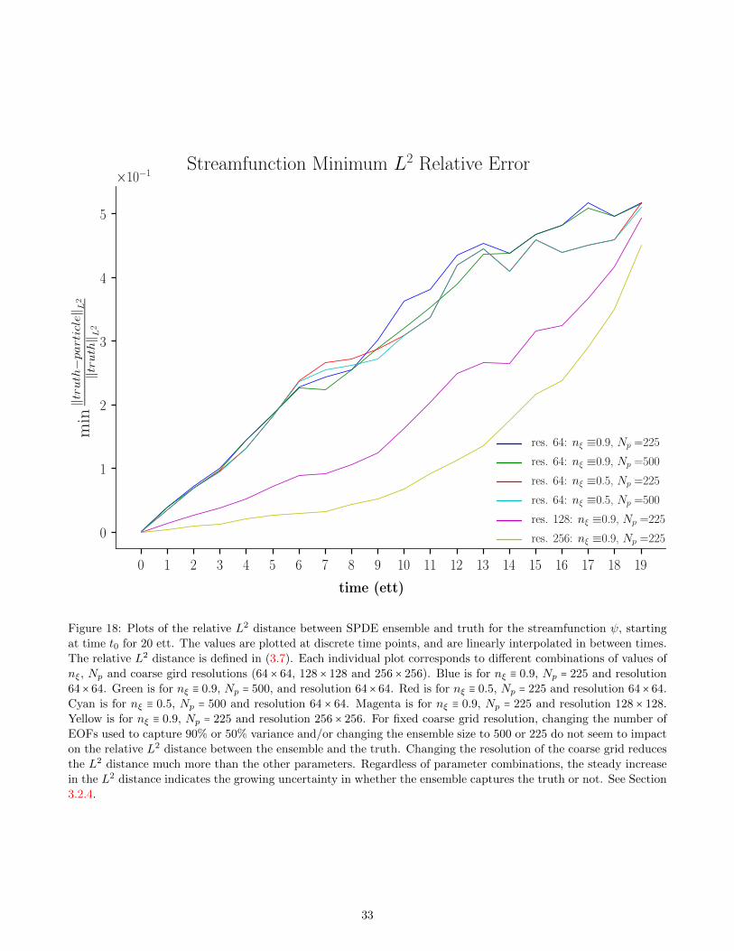
Figure 18: Plots of the relative L2 distance between SPDE ensemble and truth for the streamfunction ψ, starting
at time t0 for 20 ett. The values are plotted at discrete time points, and are linearly interpolated in between times.
The relative L2 distance is defined in (3.7). Each individual plot corresponds to different combinations of values of
nξ, Np and coarse gird resolutions (64 × 64, 128 × 128 and 256 × 256). Blue is for nξ ≡ 0.9, Np = 225 and resolution
64× 64. Green is for nξ ≡ 0.9, Np = 500, and resolution 64× 64. Red is for nξ ≡ 0.5, Np = 225 and resolution 64× 64.
Cyan is for nξ ≡ 0.5, Np = 500 and resolution 64 × 64. Magenta is for nξ ≡ 0.9, Np = 225 and resolution 128 × 128.
Yellow is for nξ ≡ 0.9, Np = 225 and resolution 256 × 256. For fixed coarse grid resolution, changing the number of
EOFs used to capture 90% or 50% variance and/or changing the ensemble size to 500 or 225 do not seem to impact
on the relative L2 distance between the ensemble and the truth. Changing the resolution of the coarse grid reduces
the L2 distance much more than the other parameters. Regardless of parameter combinations, the steady increase
in the L2 distance indicates the growing uncertainty in whether the ensemble captures the truth or not. See Section
3.2.4.
33

Figure 19: Plots of the relative L2 distance between SPDE ensemble and truth for the vorticity, starting at time
t0 for 20 ett. The values are plotted at discrete time points, and are linearly interpolated in between times. The
relative L2 distance is defined in (3.7). Each individual plot corresponds to different combinations of values of nξ,
Np and coarse gird resolutions (64 × 64, 128 × 128 and 256 × 256). Blue is for nξ ≡ 0.9, Np = 225 and resolution
64× 64. Green is for nξ ≡ 0.9, Np = 500, and resolution 64× 64. Red is for nξ ≡ 0.5, Np = 225 and resolution 64× 64.
Cyan is for nξ ≡ 0.5, Np = 500 and resolution 64 × 64. Magenta is for nξ ≡ 0.9, Np = 225 and resolution 128 × 128.
Yellow is for nξ ≡ 0.9, Np = 225 and resolution 256 × 256. For fixed coarse grid resolution, changing the number of
EOFs used to capture 90% or 50% variance and/or changing the ensemble size to 500 or 225 do not seem to impact
on the relative L2 distance between the ensemble and the truth. Changing the resolution of the coarse grid reduces
the L2 distance much more than the other parameters. Regardless of parameter combinations, the steady increase
in the L2 distance indicates the growing uncertainty in whether the ensemble captures the truth or not. See Section
3.2.4.
34

Figure 20: Plots of the relative L2 distance between SPDE ensemble and truth for the velocity, starting at time
t0 for 20 ett. The values are plotted at discrete time points, and are linearly interpolated in between times. The
relative L2 distance is defined in (3.7). Each individual plot corresponds to different combinations of values of nξ,
Np and coarse gird resolutions (64 × 64, 128 × 128 and 256 × 256). Blue is for nξ ≡ 0.9, Np = 225 and resolution
64× 64. Green is for nξ ≡ 0.9, Np = 500, and resolution 64× 64. Red is for nξ ≡ 0.5, Np = 225 and resolution 64× 64.
Cyan is for nξ ≡ 0.5, Np = 500 and resolution 64 × 64. Magenta is for nξ ≡ 0.9, Np = 225 and resolution 128 × 128.
Yellow is for nξ ≡ 0.9, Np = 225 and resolution 256 × 256. For fixed coarse grid resolution, changing the number of
EOFs used to capture 90% or 50% variance and/or changing the ensemble size to 500 or 225 do not seem to impact
on the relative L2 distance between the ensemble and the truth. Changing the resolution of the coarse grid reduces
the L2 distance much more than the other parameters. Regardless of parameter combinations, the steady increase
in the L2 distance indicates the growing uncertainty in whether the ensemble captures the truth or not. See Section
3.2.4.
35

Figure 21: Quantile-Quantile (QQ) plots for the SPDE ensemble streamfunction at time t = 4 ett, at eight obser-
vation grid (size 4 × 4) points, shown here in two separate figures of four plots each. Each plot correspond to an
individual grid point. The plot compares the ensemble quantiles to the theoretical quantiles from the Gaussian
distribution. If the ensemble is Gaussian, then we would see the plotted points (in blue) lying on the line y = x
(shown in red). The fact that the plots show fat tails give strong evidence to the fact that the ensembles are not
Gaussian. See Section 3.2.5.
Figure 22: Quantile-Quantile (QQ) plots for the SPDE ensemble vorticity at time t = 4 ett, at eight observation
grid (size 4×4) points, shown here in two separate figures of four plots each. Each plot correspond to an individual
grid point. The plot compares the ensemble quantiles to the theoretical quantiles from the Gaussian distribution.
If the ensemble is Gaussian, then we would see the plotted points (in blue) lying on the line y = x (shown in red).
The fact that the plots show fat tails give strong evidence to the fact that the ensembles are not Gaussian. See
Section 3.2.5.
36
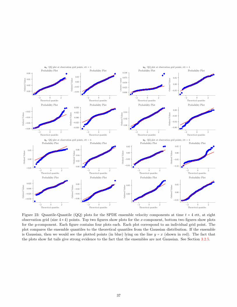
Figure 23: Quantile-Quantile (QQ) plots for the SPDE ensemble velocity components at time t = 4 ett, at eight
observation grid (size 4× 4) points. Top two figures show plots for the x-component, bottom two figures show plots
for the y-component. Each figure contains four plots each. Each plot correspond to an individual grid point. The
plot compares the ensemble quantiles to the theoretical quantiles from the Gaussian distribution. If the ensemble
is Gaussian, then we would see the plotted points (in blue) lying on the line y = x (shown in red). The fact that
the plots show fat tails give strong evidence to the fact that the ensembles are not Gaussian. See Section 3.2.5.
37

Figure 24: Box plots for the SPDE ensemble streamfunction ψ at times t = 1,2, . . . ,5 in ett, at eight observation
grid points, shown here in two separate figures of four plots each (each plot corresponds to one grid point). The
boxplots show non-symmetry and fat tails in the distribution of the ensembles, again providing strong evidence to
the fact that the ensembles are non-Gaussian.
Figure 25: Box plots for the SPDE ensemble vorticity q at times t = 1,2, . . . ,5 in ett, at eight observation grid
points, shown here in two separate figures of four plots each (each plot corresponds to one grid point). The plots
show non-symmetry and fat tails in the distribution of the ensembles, again providing strong evidence to the fact
that the ensembles are non-Gaussian.
38

Figure 26: Box plots for the SPDE ensemble velocity components, ux (top row) and uy (bottom row) at times
t = 1,2, . . . ,5 in ett, at eight observation grid points, divided into two figures of four plots each (each plot corresponds
to one grid point). The plots show non-symmetry and fat tails in the distribution of the ensembles, again providing
strong evidence to the fact that the ensembles are non-Gaussian.
39

the principles of stochastic geometric mechanics, the current work offers the first theoretically validated systematic
approach that satisfies both of these crucial ensemble-based data assimilation criteria. The trajectories of the
particles in the ensemble arise from a decomposition of the true (deterministic) fluid velocity into a drift velocity
and a (Stratonovich) stochastic perturbation at the coarse resolution. The equations for the drift velocity arise
from stationary variations of Hamilton’s principle for ideal fluid dynamics, constrained to follow the stochastic
Lagrangian paths whose spatial correlations are determined from the present methodology. Thus, derived via
fundamental principles of stochastic geometric mechanics, the present methodology has produced successful results
for uncertainty quantification.
The ensembles produced by the methodology presented here will be used in further work to forecast the future
position of the true trajectory. An additional mechanism will correct the ensemble by selecting and multiplying
the more likely particles and casting out those that are too far from the true solution. This “pruning” procedure
to correct, or refine the ensemble will be based on partial (sparse/noisy) observations. The correction mechanism
assimilates the data into the system and reduces the model uncertainty. Accomplishing this forecast will be a
challenging task, because the dimensionality of the system will remain high, even after applying the coarsening
using the methodology developed here. The authors will report progress toward accomplishing such forecasts in a
sequel to the present paper.
Acknowledgements
The authors thank The Engineering and Physical Sciences Research Council (EPSRC) for their support of this
work through the grant EP/N023781/1. The authors also thank Pavel Berloff, Mike Cullen, John Gibbon, Georg
Gottwald, Nikolas Kantas, Etienne Memin, Sebastian Reich, Valentin Resseguier, and Aretha Teckentrup for the
many useful, constructive discussions held with them throughout the preparation of this work.
References
Balay, S., Abhyankar, S., Adams, M. F., Brown, J., Brune, P., Buschelman, K., Dalcin, L., Eijkhout, V., Gropp,
W. D., Kaushik, D., Knepley, M. G., McInnes, L. C., Rupp, K., Smith, B. F., Zampini, S., Zhang, H., and Zhang,
H. (2016). PETSc users manual. Technical Report ANL-95/11 - Revision 3.7, Argonne National Laboratory.
Balay, S., Gropp, W. D., McInnes, L. C., and Smith, B. F. (1997). Efficient management of parallelism in object
oriented numerical software libraries. In Arge, E., Bruaset, A. M., and Langtangen, H. P., editors, Modern
Software Tools in Scientific Computing, pages 163–202. Birkhauser Press.
Beale, J., Kato, T., and Majda, A. (1984). Remarks on the breakdown of smooth solutions for the 3-D Euler
equations. Com. Math. Phys., 94:61–66.
Bernsen, E., Bokhove, O., and van der Vegt, J. J. (2006). A (dis)continuous finite element model for generalized
2D vorticity dynamics. J. Comput. Phys., 211(2):719–747.
Beskos, A., Crisan, D., Jasra, A., Kamatani, K., and Zhou, Y. (2017). A stable particle filter for a class of
high-dimensional state-space models. Advances in Applied Probability, 49(1):2448.
Brzezniak, Z., Flandoli, F., and Maurelli, M. (2016). Existence and uniqueness for stochastic 2D Euler flows with
bounded vorticity. Archive for Rational Mechanics and Analysis, 221:107–142.
Cotter, C., Gottwald, G., and Holm, D. D. (2017). Stochastic partial differential fluid equations as a diffusive limit
of deterministic Lagrangian multi-time dynamics. arXiv: 1706.00287 [math.AP].
Crisan, D., Flandoli, F., and Holm, D. D. (2017). Solution properties of a 3D stochastic Euler fluid equation. arXiv:
1704.06989 [math-ph].
Crisan, D. and Lang, O. (2018). Well-posedness for 2D Euler equations with stochastic Lie transport noise. In
preparation.
40
Dalcin, L. D., Paz, R. R., Kler, P. A., and Cosimo, A. (2011). Parallel distributed computing using Python.
Advances in Water Resources, 34(9):1124–1139. New Computational Methods and Software Tools.
Gay-Balmaz, F. and Holm, D. D. (2018). Stochastic geometric models with non-stationary spatial correlations in
Lagrangian fluid flows. Journal of Nonlinear Science, 28(3):873–904.
Gottlieb, S. (2005). On high order strong stability preserving Runge–Kutta and multi step time discretizations. J.
Sci. Comput., 25(1):105–128.
Hannachi, A. (2004). A primer for EOF analysis of climate data.
Hannachi, A., Jolliffe, I., and Stephenson, D. (2007). Empirical orthogonal functions and related techniques in
atmospheric science: A review. Int. J. Climatol., 27:1119–1152.
Holm, D. D. (2011). Geometric Mechanics, Part 1 and Part 2. World Scientific, 2nd Ed.
Holm, D. D. (2015). Variational principles for stochastic fluids. Proc. Roy. Soc. A, 471.
Holm, D. D., Marsden, J., and Ratiu, T. (1998). The Euler–Poincare equations and semidirect products with
applications to continuum theories. Adv. in Math., 137:1–81.
Holm, D. D., Schmah, T., and Stoica, C. (2009). Geometric Mechanics and Symmetry: From Finite to Infinite
Dimensions. Oxford University Press.
Koch, I. (2013). Analysis of multivariate and high-dimensional data, volume 32. Cambridge University Press.
Lang, A. (2010). A Lax equivalence theorem for stochastic differential equations. Journal of Computational and
Applied Mathematics, 234(12):3387–3396.
Marsden, J. and Ratiu, T. (1999). Introduction to Mechanics and Symmetry. Springer, 2nd Ed.
Memin, E. (2014). Fluid flow dynamics under location uncertainty. Geophys. Astro. Fluid, 108:119–146.
Mikulevicius, R. and Rozovskii, B. (2004). Stochastic Navier–Stokes equations for turbulent flows. SIAM J. Math.
Anal., 35:1250–1310.
Pardoux, E. (2007). Stochastic Partial Differential Equations. Lectures given in Fudan University, Shanghai. Mar-
seille, France.
Rathgeber, F., Ham, D. A., Mitchell, L., Lange, M., Luporini, F., McRae, A. T. T., Bercea, G.-T., Markall, G. R.,
and Kelly, P. H. J. (2016). Firedrake: automating the finite element method by composing abstractions. ACM
Trans. Math. Softw., 43(3):24:1–24:27.
Schaumloffel, K.-U. (1988). White noise in space and time and the cylindrical Wiener process. Stoch. Anal. Appl.,
6:81–89.
She, Z.-S. (1991). Intermittency and non-gaussian statistics in turbulence. Fluid Dynamics Research, 8(1-4):143.
41