Embed Size (px)
Citation preview
/66
AntoineCornuéjols
AgroParisTech–INRAMIA518
CollaboraDvefiltering
Automa'crecommenda'ons
hGp://www.agroparistech.fr/ufr-info/membres/cornuejols/Teaching/Master-AIC/M2-AIC-advanced-ML.html
/66
IntroducDon
ThecollaboraDvefilteringproblem
2«CollaboraDvefiltering»(A.Cornuéjols)
/66
History
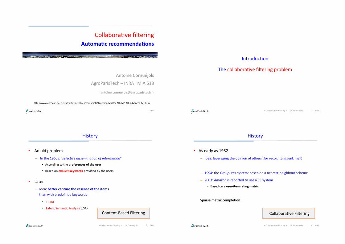
• Anoldproblem
– Inthe1960s:“selec%vedissemina%onofinforma%on”
• Accordingtothepreferencesoftheuser
• Basedonexplicitkeywordsprovidedbytheusers
• Later– Idea:be9ercapturetheessenceoftheitems
thanwithpredefinedkeywords
• TF-IDF
• LatentSemanDcAnalysis(LSA)
3«CollaboraDvefiltering»(A.Cornuéjols)
Content-BasedFiltering
/66
History
• Asearlyas1982– Idea:leveragingtheopinionofothers(forrecognizingjunkmail)
– 1994:theGroupLenssystem:basedonanearest-neighbourscheme
– 2003:AmazonisreportedtouseaCFsystem
• Basedonauser-itemra'ngmatrix
Sparsematrixcomple'on
4«CollaboraDvefiltering»(A.Cornuéjols)
CollaboraDveFiltering
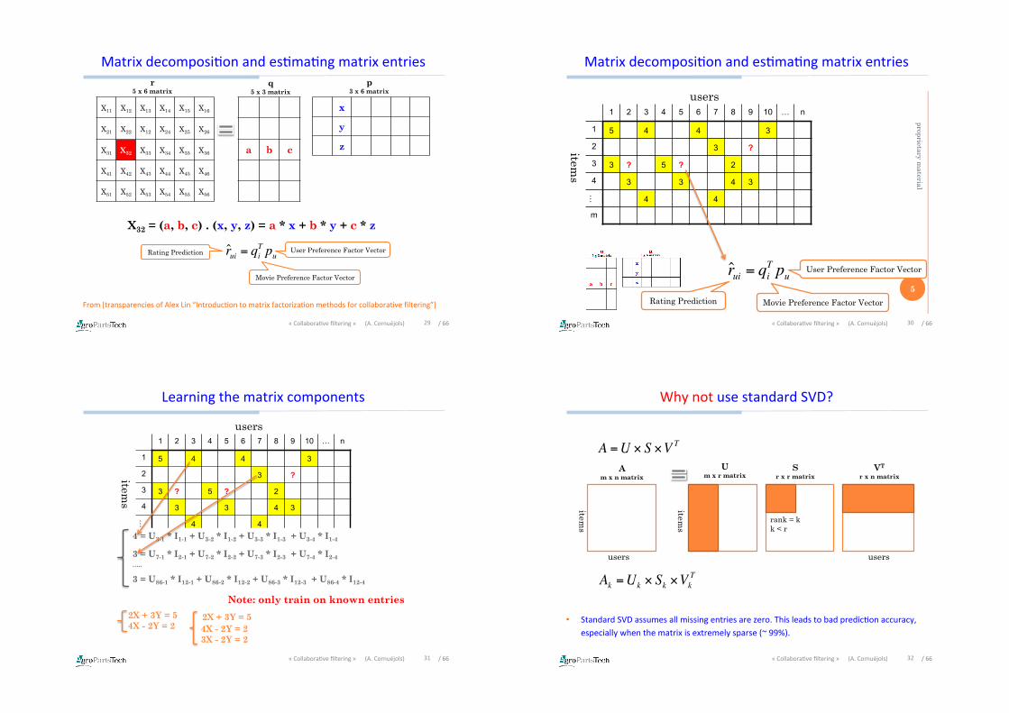
/66
History
• TheNe>lixPrizein2006
– Amillion-dollarprizeforthefirstteamtodemonstrateasystemthat
outperformedthein-housesystembymorethan10%onRMSE
– Datasetwith100,000,000realcustomerraDngs
– Morethan5,000teamsregistered
– Prizeawardedin2009
5«CollaboraDvefiltering»(A.Cornuéjols) /66
Examples
• Amazon
• GoogleNews
– recommendsarDclesbasedonclickand
searchhistory
– Millionsofusers/millionsofarDcles
6«CollaboraDvefiltering»(A.Cornuéjols)
Intro Prelim Class/Reg MF Extend Combo Conclude
Collaborative Filtering in the Wild...
Amazon.com recommends products based on purchasehistory
Linder et al., 2003
Lester Mackey Collaborative Filtering
Intro Prelim Class/Reg MF Extend Combo Conclude
Collaborative Filtering in the Wild...
• Google Newsrecommends newarticles based onclick and searchhistory
• Millions of users,millions of articles
Das et al., 2007
Lester Mackey Collaborative Filtering
/66
IntroducDon
torecommendingsystems
7«CollaboraDvefiltering»(A.Cornuéjols) /66
TheNeflixprize
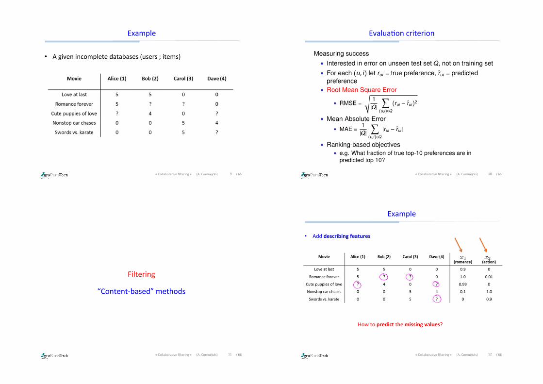
• Adatabaseof≈25,000movies
• Approximately500,000users
• Over100.106raDngs(from1to5)(≈200/user)
Ø Predictthemissingra'ngs(≈12.109missingvalues!!)
8«CollaboraDvefiltering»(A.Cornuéjols)
users
Items(movies)
Knownvalues
/66
Example
• Agivenincompletedatabases(users;items)
9«CollaboraDvefiltering»(A.Cornuéjols) /66
EvaluaDoncriterion
10«CollaboraDvefiltering»(A.Cornuéjols)
Intro Prelim Class/Reg MF Extend Combo Conclude
What is Collaborative Filtering?
Measuring success• Interested in error on unseen test set Q, not on training set• For each (u, i) let rui = true preference, r̂ui = predicted
preference• Root Mean Square Error
• RMSE =s
1|Q|X
(u,i)2Q(rui � r̂ui)2
• Mean Absolute Error• MAE =
1|Q|X
(u,i)2Q|rui � r̂ui |
• Ranking-based objectives• e.g. What fraction of true top-10 preferences are in
predicted top 10?
Lester Mackey Collaborative Filtering
/66
Filtering
“Content-based”methods
11«CollaboraDvefiltering»(A.Cornuéjols) /66
Example
• Adddescribingfeatures
12«CollaboraDvefiltering»(A.Cornuéjols)
Howtopredictthemissingvalues?
/66
Example
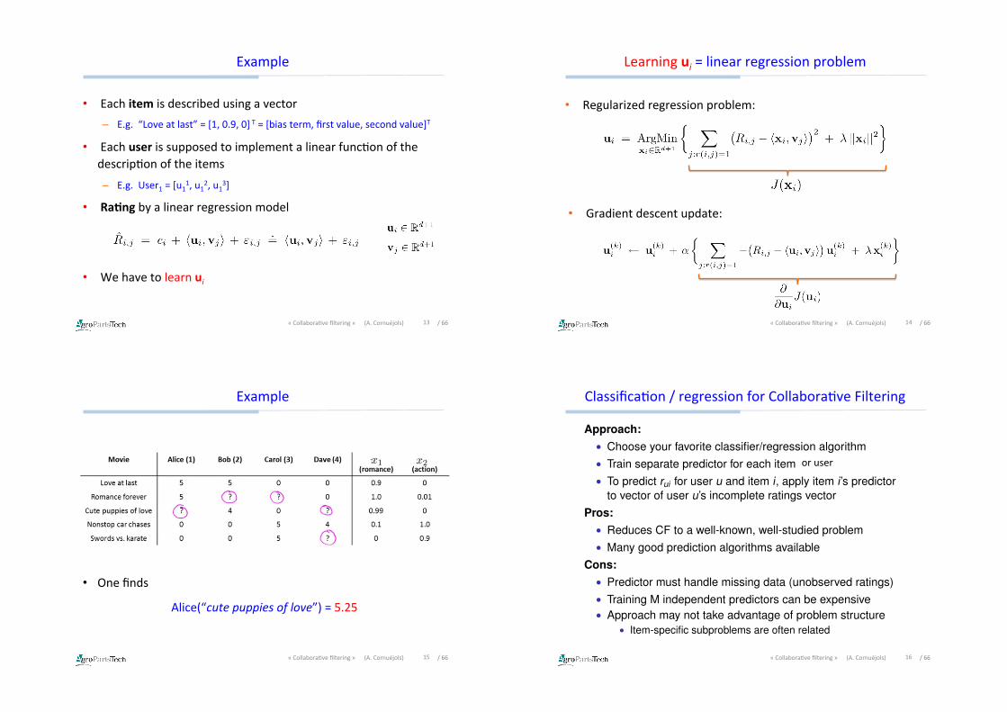
• Eachitemisdescribedusingavector– E.g.“Loveatlast”=[1,0.9,0]T=[biasterm,firstvalue,secondvalue]T
• EachuserissupposedtoimplementalinearfuncDonofthe
descripDonoftheitems
– E.g.User1=[u11,u12,u13]
• Ra'ngbyalinearregressionmodel
• Wehavetolearnui
13«CollaboraDvefiltering»(A.Cornuéjols) /66
Learningui=linearregressionproblem
• Regularizedregressionproblem:
14«CollaboraDvefiltering»(A.Cornuéjols)
• Gradientdescentupdate:
/66
Example
• Onefinds
Alice(“cutepuppiesoflove”)=5.25
15«CollaboraDvefiltering»(A.Cornuéjols) /66
ClassificaDon/regressionforCollaboraDveFiltering
16«CollaboraDvefiltering»(A.Cornuéjols)
Intro Prelim Class/Reg MF Extend Combo Conclude Naive Bayes KNN
Classification/Regression for CF
Approach:• Choose your favorite classifier/regression algorithm• Train separate predictor for each item• To predict rui for user u and item i, apply item i’s predictor
to vector of user u’s incomplete ratings vectorPros:• Reduces CF to a well-known, well-studied problem• Many good prediction algorithms available
Cons:• Predictor must handle missing data (unobserved ratings)• Training M independent predictors can be expensive• Approach may not take advantage of problem structure
• Item-specific subproblems are often related
Lester Mackey Collaborative Filtering
oruser
/66
Conclusionsaboutcontent-basedfiltering
• Notreallycollabora've
• Requiresthatrelevantfeaturesbegiventocharacterizetheitems(e.g.movies)
• Requiresthatitemsbecharacterizedusingthesefeatures
17«CollaboraDvefiltering»(A.Cornuéjols) /66
CollaboraDvefiltering
“Neibourhood”methods
18«CollaboraDvefiltering»(A.Cornuéjols)
/66
Principle
• User-basedapproach
1. Computessimilari'esbetweenthegivenuserandeveryotherusers
2. IdenDfynearestneighborsofthegivenuser
3. Computethemissingvalue(s)usingaweightedscorefromtheneighbor
users
Requiresameasureofsimilaritybetweenusers
19«CollaboraDvefiltering»(A.Cornuéjols) /66
Example
• Database
20«CollaboraDvefiltering»(A.Cornuéjols)
/66
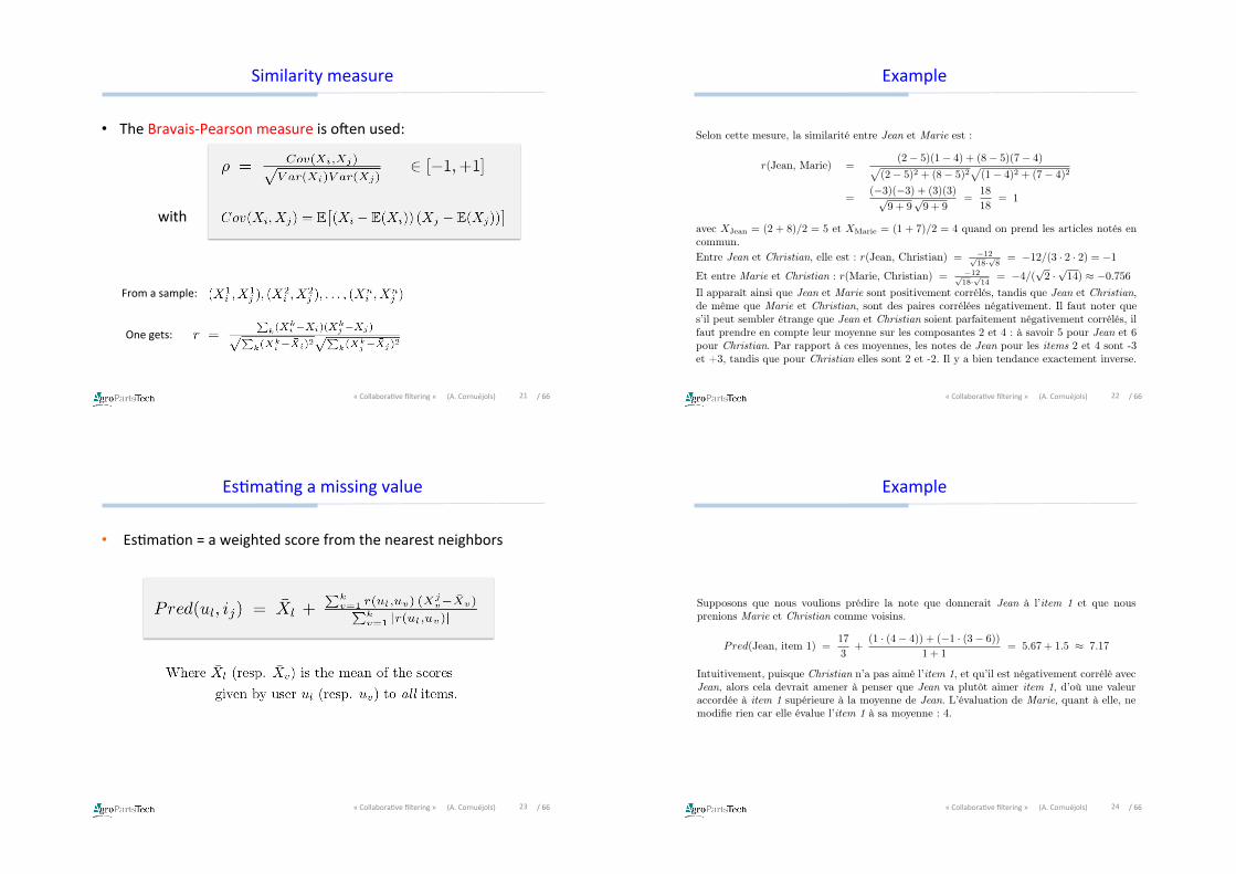
Similaritymeasure
• TheBravais-Pearsonmeasureisosenused:
21«CollaboraDvefiltering»(A.Cornuéjols)
with
Fromasample:
Onegets:
/66
Example
688 PARTIE 5 : Au-delà de l’apprentissage supervisé
scores élevés pour la première variable auront tendance à avoir des scores faibles pour la deuxièmeet inversement.
En disposant d’un échantillon de taille n, (X1i , X
1j ), (X
2i , X
2j ), . . . , (X
ni , X
nj ) tiré d’une distri-
bution conjointe, la quantité :
r =
�k(X
ki � X̄i)(Xk
j � X̄j)⇤�k(X
ki � X̄i)2
⇤�k(X
kj � X̄j)2
est une estimation de �.
Exemple Calcul de la similaritéSelon cette mesure, la similarité entre Jean et Marie est :
r(Jean, Marie) =(2� 5)(1� 4) + (8� 5)(7� 4)⇥
(2� 5)2 + (8� 5)2⇥(1� 4)2 + (7� 4)2
=(�3)(�3) + (3)(3)⇤
9 + 9⇤9 + 9
=18
18= 1
avec XJean = (2 + 8)/2 = 5 et XMarie = (1 + 7)/2 = 4 quand on prend les articles notés encommun.Entre Jean et Christian, elle est : r(Jean, Christian) = �12⇥
18·⇥8
= �12/(3 · 2 · 2) = �1
Et entre Marie et Christian : r(Marie, Christian) = �12⇥18·
⇥14
= �4/(⇤2 ·
⇤14) ⇥ �0.756
Il apparaît ainsi que Jean et Marie sont positivement corrélés, tandis que Jean et Christian,de même que Marie et Christian, sont des paires corrélées négativement. Il faut noter ques’il peut sembler étrange que Jean et Christian soient parfaitement négativement corrélés, ilfaut prendre en compte leur moyenne sur les composantes 2 et 4 : à savoir 5 pour Jean et 6pour Christian. Par rapport à ces moyennes, les notes de Jean pour les items 2 et 4 sont -3et +3, tandis que pour Christian elles sont 2 et -2. Il y a bien tendance exactement inverse.
De fait, il a été empiriquement observé que la corrélation de Pearson n’est pas la mesure decorrélation la mieux adaptée pour le filtrage collaboratif, un meilleur choix étant de prendrela corrélation de Pearson à la puissance 2.5 [BHK98].
Calcul d’une recommandation
La plupart des algorithmes de recommandations utilisent une combinaison des évaluationsd’utilisateurs proches au sens de la mesure de similarité employée. Par exemple, l’approche laplus simple consiste à retenir les k plus proches voisins au sens de cette similarité r et de calculerune moyenne pondérée de leurs évaluations pour fournir une prédiction d’utilité.
Pred(ul, ij) = X̄l +
�kv=1 r(ul, uv) (X
jv � X̄v)�k
v=1 |r(ul, uv)|(20.11)
où X̄l (resp. X̄v) est la moyenne des notes attribuées par l’utilisateur ul (resp. uv) à tous lesitems.
22«CollaboraDvefiltering»(A.Cornuéjols)
/66
EsDmaDngamissingvalue
• EsDmaDon=aweightedscorefromthenearestneighbors
23«CollaboraDvefiltering»(A.Cornuéjols) /66
Example
Chapitre 20 Vers de nouvelles tâches et de nouvelles questions 689
Exemple Calcul d’une recommandationSupposons que nous voulions prédire la note que donnerait Jean à l’item 1 et que nousprenions Marie et Christian comme voisins.
Pred(Jean, item 1) =17
3+
(1 · (4� 4)) + (�1 · (3� 6))
1 + 1= 5.67 + 1.5 ⇤ 7.17
Intuitivement, puisque Christian n’a pas aimé l’item 1, et qu’il est négativement corrélé avecJean, alors cela devrait amener à penser que Jean va plutôt aimer item 1, d’où une valeuraccordée à item 1 supérieure à la moyenne de Jean. L’évaluation de Marie, quant à elle, nemodifie rien car elle évalue l’item 1 à sa moyenne : 4.
L’approche centrée items est duale de l’approche centrée utilisateurs. Elle consiste en e�et àutiliser une mesure de similarité entre items pour déterminer les k items les plus similaires à l’itemij pour lequel on cherche à calculer Pred(ul, ij). On utilise alors une formule de pondération qui,dans le cas le plus simple, est :
Pred(ul, ij) = X̄i +
�kv=1 r(ij , iv) (X
vl � X̄v)
�kv=1 |r(ij , iv)|
(20.12)
ExempleSupposons que nous voulions prédire la note que donnerait Jean à l’item 1 et que nousprenions Item 2 et Item 4 comme voisins (Item 3 ne peut pas être voisin de Item 1 car il nepartage aucune composante utilisateur).En utilisant la mesure de corrélation de Pearson, on trouve que r(Item 1, Item 2) = �1 etr(Item 1, Item 4) = 1. On a alors :
Pred(Jean, Item 1) =4 + 3
2+
(�1 · (2� 11/3)) + (1 · (8� 19/3))
1 + 1⇤ 3.5 + 1.67 = 5.17
On observe que, en utilisant ces formules de similarité et de combinaison, le résultat n’estpas le même que dans l’approche centrée utilisateur.
5.2 Les di�cultés
Les di⇥cultés liées au filtrage collaboratif proviennent essentiellement :• de la dimension de la matrice utilisateurs-items qui peut éventuellement être énorme (typi-
quement de l’ordre de 104 lignes ⇥105 colonnes) ;• du caractère creux de cette matrice (typiquement avec moins de 1 % d’entrées) ;• du choix à e�ectuer de la mesure de similarité, en particulier si les données comportent des
relations.Par ailleurs, il n’est pas facile de mesurer la performance d’un système de filtrage-collaboratif,
ce qui est nécessaire pour identifier la technique la mieux adaptée à une tâche particulière.
5.2.1 Traitement des matrices
Afin de traiter de très grandes matrices, dans lesquelles la liste des items est relativement peuvariable comparée à la liste des utilisateurs, plusieurs techniques sont employées.
L’une d’elles consiste à précalculer les voisins dans l’espace des items (peu variables) afin delimiter les calculs en ligne de pred(ul, ij). Une autre consiste à e�ectuer une classification non
24«CollaboraDvefiltering»(A.Cornuéjols)
/66
Item-centeredtechnique
• Thesametechniquecanbeusedonitemsinsteadofusers
25«CollaboraDvefiltering»(A.Cornuéjols) /66
Conclusions
• Difficultdueto
– Highdimensionalityofthematrix
– Highnumberofitems
– Highnumberofusers
– Thesimilaritymustbecomputedforallusers(oritems)
26«CollaboraDvefiltering»(A.Cornuéjols)
/66
CollaboraDvefiltering
Matrixcomple'onmethods
27«CollaboraDvefiltering»(A.Cornuéjols) /66
NoDonoflatentvariablesLatent variable view
Geared towards females
Geared towards males
serious
escapist
The PrincessDiaries
The Lion King
Braveheart
Lethal Weapon
Independence Day
AmadeusThe Color Purple
Dumb and Dumber
��������11
Sense and Sensibility
Gus
Dave
Latent factor models
28«CollaboraDvefiltering»(A.Cornuéjols)
/66
MatrixdecomposiDonandesDmaDngmatrixentries
From[transparenciesofAlexLin“IntroducDontomatrixfactorizaDonmethodsforcollaboraDvefiltering”]
29«CollaboraDvefiltering»(A.Cornuéjols)
Refresher: Matrix Decomposition
a b c
x
y
z
p 3 x 6 matrix
X11 X12 X13 X14 X15 X16
X21 X22 X12 X24 X25 X26
X31 X32 X33 X34 X35 X36
X41 X42 X43 X44 X45 X46
X51 X52 X53 X54 X55 X56
r 5 x 6 matrix
X32 = (a, b, c) . (x, y, z) = a * x + b * y + c * z
q 5 x 3 matrix
!
ˆ r ui = qiT pu 4
Movie Preference Factor Vector
User Preference Factor Vector Rating Prediction
proprietary material
/66
MatrixdecomposiDonandesDmaDngmatrixentries
Making Prediction as Filling Missing Value
n … 10 9 8 7 6 5 4 3 2 1
3 4 4 5 1
? 3 2
2 ? 5 ? 3 3
3 4 3 3 4
4 4
…
m
users
items
5
!
ˆ r ui = qiT pu
Movie Preference Factor Vector
User Preference Factor Vector
Rating Prediction
proprietary material
30«CollaboraDvefiltering»(A.Cornuéjols)
/66
LearningthematrixcomponentsLearn Factor Vectors
n … 10 9 8 7 6 5 4 3 2 1
3 4 4 5 1
? 3 2
2 ? 5 ? 3 3
3 4 3 3 4
4 4
…
m
users
items
4 = U3-1 * I1-1 + U3-2 * I1-2 + U3-3 * I1-3 + U3-4 * I1-4
3 = U7-1 * I2-1 + U7-2 * I2-2 + U7-3 * I2-3 + U7-4 * I2-4 …..
3 = U86-1 * I12-1 + U86-2 * I12-2 + U86-3 * I12-3 + U86-4 * I12-4
2X + 3Y = 5 4X - 2Y = 2 3X - 2Y = 2
2X + 3Y = 5 4X - 2Y = 2
6
proprietary material
Note: only train on known entries
31«CollaboraDvefiltering»(A.Cornuéjols) /66
WhynotusestandardSVD?
• StandardSVDassumesallmissingentriesarezero.ThisleadstobadpredicDonaccuracy,
especiallywhenthematrixisextremelysparse(~99%).
32«CollaboraDvefiltering»(A.Cornuéjols)
Singular Value Decomposition (SVD)
!
Ak =Uk " Sk "VkT
!
A =U " S "VT
A m x n matrix
users
items
VT r x n matrix
U m x r matrix
S r x r matrix
items
users
rank = k k < r
20
proprietary material
/66
Learningthematrixcomponents
• rui:actualraDngforuseruonitemi
• xui:predictedraDngforuseruonitemi
33«CollaboraDvefiltering»(A.Cornuéjols)
How to Learn Factor Vectors ! How do we learn preference factor vectors (a, b, c) and
(x, y, z)? ! Minimize errors on the known ratings
8
!
minq*.p*
(rui " xui)2
(u,i)#k$ To learn the factor
vectors (pu and qi)
Minimizing Cost Function (Least Squares Problem)
rui : actual rating for user u on item I xui : predicted rating for user u on item I
proprietary material
/66
DatanormalizaDonData Normalization ! Remove Global mean
n … 10 9 8 7 6 5 4 3 2 1
.49 -.2 -.9 1.5 1
? .79 2
-.4 ? .46 ? 0.6 3
.69 .76 .82 .39 4
.8 .52
…
m
users
items
9
proprietary material
34«CollaboraDvefiltering»(A.Cornuéjols)
/66
FactorisaDonmodel
35«CollaboraDvefiltering»(A.Cornuéjols)
Factorization Model
rui : actual rating of user u on item I u : training rating average bu : user u user bias bi : item i item bias qi : latent factor array of item i pu : later factor array of user u
10
To learn the factor vectors (pu and qi)
! Only Preference factors
!
minq*.p*
(rui "µ " qiT pu)
2
(u,i)#k$
Global Mean
Preference Factor
Rating = 4
proprietary material
• rui:actualraDngofuseruonitemi
• u:trainingraDngaverage
• bu:useruuserbias
• bi:itemiitembias
• qi:latentfactorarrayofitemI
• pu:latentfactorarrayofuseru
/66
Additembiasanduserbias
36«CollaboraDvefiltering»(A.Cornuéjols)
Adding Item Bias and User Bias
!
minq*.p*
(rui "µ " bi " bu " qiT pu)
2
(u,i)#k$
rui : actual rating of user u on item I u : training rating average bu : user u user bias bi : item i item bias qi : latent factor array of item i pu : later factor array of user u
11
! Add Item bias and User bias as parameters
To learn Item bias and User bias
Global Mean
Preference Factor
Rating = 4
Item Bias User Bias
proprietary material
• rui:actualraDngofuseruonitemi
• u:trainingraDngaverage
• bu:useruuserbias
• bi:itemiitembias
• qi:latentfactorarrayofitemI
• pu:latentfactorarrayofuseru
/66
RegularizaDon
37«CollaboraDvefiltering»(A.Cornuéjols)
Topreventmodeloverfixng
Regularization ! To prevent model overfitting
!
minq*.p*
(rui "µ " bi " bu " qiT pu)
2 + #( qi2
+ pu2
+ bi2 + bu
2)(u,i)$k%
rui : actual rating of user u on item I u : training rating average bu : user u user bias bi : item i item bias qi : latent factor array of item i pu : later factor array of user u : regularization Parameters
!
"
12
Regularization to prevent overfitting
Global Mean
Preference Factor
Rating = 4
Item Bias User Bias
proprietary material
• rui:actualraDngofuseruonitemi
• u:trainingraDngaverage
• bu:useruuserbias
• bi:itemiitembias
• qi:latentfactorarrayofitemI
• pu:latentfactorarrayofuseru
/66
OpDmizefactorvectors
• FindopDmalfactorvectors–minimizingcostfuncDon
• Algorithms
– Stochas'cgradientdescent:mostfrequentlyused
– Others:alternaDngleastsquares,…
38«CollaboraDvefiltering»(A.Cornuéjols)
Risk Minimization View• Objective Function
• Stochastic gradient descent
• No need for locking• Multicore updates asynchronously
(Recht, Re, Wright, 2012 - Hogwild)
minimizep,q
X
(u,i)2S
(rui � hpu, qii)2 + �hkpk2
Frob
+ kqk2Frob
i
muchfaster
pu (1� ⇥�t)pu � �tqi(rui � hpu, qii)qi (1� ⇥�t)qi � �tpu(rui � hpu, qii)
/66
MatrixfactorizaDontuning
• Numberoffactors(latentvariables)inthepreferencevectors
• LearningrateofGradientDescent
– Bestresultsusuallycomingfromdifferentlearningratesfordifferent
parameters.Especiallyuser/itembiasterms
• ParametersinfactorizaDonmodel
– Timedependentparameters
– Seasonalitydependentparameters
• ManyotherconsideraDons
39«CollaboraDvefiltering»(A.Cornuéjols) /66
Learningthematrixcomponents
• Byatwo-stepprocedurerepeatedmanyDmes=coordinategradientdescent
– First,esDmatetheuser’spreferencevectors,givenasetofitem’svectors
– Second,esDmatetheitem’svectors,giventheuser’spreferencevectors
40«CollaboraDvefiltering»(A.Cornuéjols)
Risk Minimization View• Objective Function
• Alternating least squares
minimizep,q
X
(u,i)2S
(rui � hpu, qii)2 + �hkpk2
Frob
+ kqk2Frob
i
pu
2
4�1+X
i|(u,i)⇥S
qiq⇤i
3
5�1
X
i
qirui
qi
2
4�1+X
u|(u,i)⇥S
pup⇤u
3
5�1
X
i
purui
good forMapReduce
/66
IllustraDon
E
41«CollaboraDvefiltering»(A.Cornuéjols) /66
IllustraDon
E
42«CollaboraDvefiltering»(A.Cornuéjols)
/66
IllustraDon
E
43«CollaboraDvefiltering»(A.Cornuéjols) /66
IllustraDon
E
44«CollaboraDvefiltering»(A.Cornuéjols)
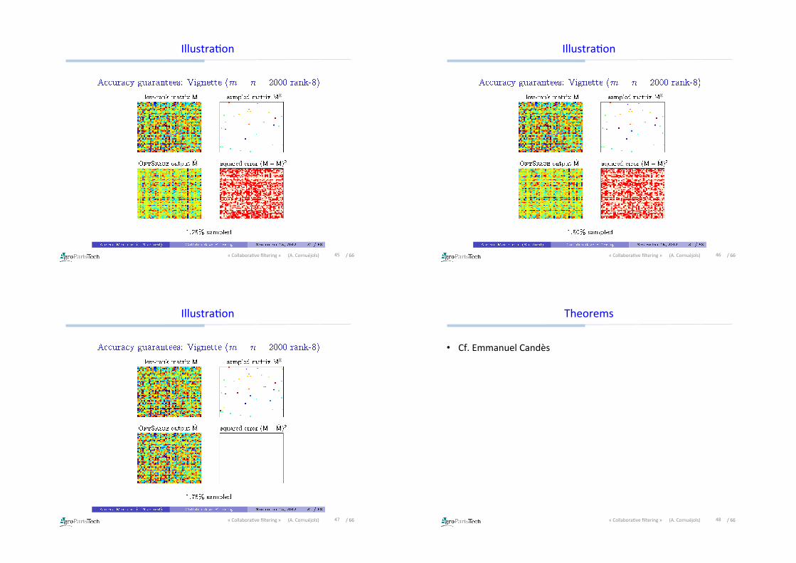
/66
IllustraDon
E
45«CollaboraDvefiltering»(A.Cornuéjols) /66
IllustraDon
E
46«CollaboraDvefiltering»(A.Cornuéjols)
/66
IllustraDon
E
47«CollaboraDvefiltering»(A.Cornuéjols) /66
Theorems
• Cf.EmmanuelCandès
48«CollaboraDvefiltering»(A.Cornuéjols)
/66
Ranking
49«CollaboraDvefiltering»(A.Cornuéjols) /66
Theproblem
• Wehaveasetof“objects”xi∈X
• WewantarankingonX
WesupposethatthereexistsatrainingsetEofpairs(u,v)∈XxXst.
– u>v(upreferredtov)orv<u
– Everyx∈XappearsatleastonceinE
Welookforafunc'onF:X→ℜst.u<viffF(u)>F(v)
50«CollaboraDvefiltering»(A.Cornuéjols)
/66
Rankingsandpreferencegraphs
Totalorder
51«CollaboraDvefiltering»(A.Cornuéjols)
“48740_7P_8291_011.tex” — 10/1/2012 — 17:41 — page 344
344 11 Learning to Rank
(a) (b)
(c) (d)
Figure 11.1Four sample feedback graphs. The vertices are instances, and the edges are the preference pairs indicating thatone instance should be ranked above the other.
Such inconsistent feedback is analogous to receiving the same example with contradictorylabels in the classification setting.
As noted earlier, the aim of the learning algorithm is to find a good ranking over the entiredomain X . Formally, we represent such a ranking by a real-valued function F : X → Rwith the interpretation that F ranks v above u if F(v) > F(u). Note that the actual numericalvalues of F are immaterial; only the relative ordering that they define is of interest (althoughthe algorithms that we describe shortly will in fact use these numerical values as part of thetraining process).
To quantify the “goodness” of a ranking F with respect to the given feedback, we computethe fraction of preference-pair misorderings:
1|E|
!
(u,v)∈E1{F(v) ≤ F(u)} .
Bipar'tegraph
Allelementsofone
setarepreferredto
everyelementsof
theotherset
“48740_7P_8291_011.tex” — 10/1/2012 — 17:41 — page 344
344 11 Learning to Rank
(a) (b)
(c) (d)
Figure 11.1Four sample feedback graphs. The vertices are instances, and the edges are the preference pairs indicating thatone instance should be ranked above the other.
Such inconsistent feedback is analogous to receiving the same example with contradictorylabels in the classification setting.
As noted earlier, the aim of the learning algorithm is to find a good ranking over the entiredomain X . Formally, we represent such a ranking by a real-valued function F : X → Rwith the interpretation that F ranks v above u if F(v) > F(u). Note that the actual numericalvalues of F are immaterial; only the relative ordering that they define is of interest (althoughthe algorithms that we describe shortly will in fact use these numerical values as part of thetraining process).
To quantify the “goodness” of a ranking F with respect to the given feedback, we computethe fraction of preference-pair misorderings:
1|E|
!
(u,v)∈E1{F(v) ≤ F(u)} .
Layeredfeedback
“48740_7P_8291_011.tex” — 10/1/2012 — 17:41 — page 344
344 11 Learning to Rank
(a) (b)
(c) (d)
Figure 11.1Four sample feedback graphs. The vertices are instances, and the edges are the preference pairs indicating thatone instance should be ranked above the other.
Such inconsistent feedback is analogous to receiving the same example with contradictorylabels in the classification setting.
As noted earlier, the aim of the learning algorithm is to find a good ranking over the entiredomain X . Formally, we represent such a ranking by a real-valued function F : X → Rwith the interpretation that F ranks v above u if F(v) > F(u). Note that the actual numericalvalues of F are immaterial; only the relative ordering that they define is of interest (althoughthe algorithms that we describe shortly will in fact use these numerical values as part of thetraining process).
To quantify the “goodness” of a ranking F with respect to the given feedback, we computethe fraction of preference-pair misorderings:
1|E|
!
(u,v)∈E1{F(v) ≤ F(u)} .
Arbitraryfeedback
(withintransiDve
preferences)
/66
OpDmizaDoncriteria
• Empiricalrankingloss
• RankinglossofFwrt.adistribuDonDoverE
52«CollaboraDvefiltering»(A.Cornuéjols)
[rloss(F ) =
1
|E|X
(u,v)2E
1�F (v) F (u)
rlossD(F ).
=X
(u,v)2X⇥X
D(u, v) 1�F (v) F (u)
= P(u,v)⇠D
⇥F (v) F (u)
⇤
/66
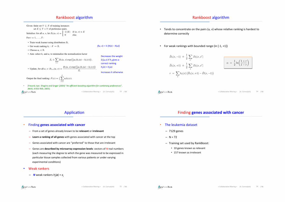
Rankboostalgorithm
• [Freund,Iyer,ShapireandSinger(2003)“Anefficientboos%ngalgorithmforcombiningpreferences”,JMLR,4:933-969,2003]
53«CollaboraDvefiltering»(A.Cornuéjols)
“48740_7P_8291_011.tex” — 10/1/2012 — 17:41 — page 346
346 11 Learning to Rank
Algorithm 11.1The RankBoost algorithm, using a pair-based weak learner
Given: finite set V ⊆ X of training instancesset E ⊆ V ×V of preference pairs.
Initialize: for all u, v, let D1(u, v) =!
1/|E| if (u, v) ∈ E
0 else.For t = 1, . . . , T :
• Train weak learner using distribution Dt .• Get weak ranking ht : X → R.• Choose αt ∈ R.• Aim: select ht and αt to minimalize the normalization factor
Zt.="
u,v
Dt (u, v) exp# 1
2αt (ht (u)−ht (v))$.
• Update, for all u, v: Dt+1(u, v) = Dt(u, v) exp# 1
2αt (ht (u)−ht (v))$
Zt
.
Output the final ranking: F(x) = 12
T"
t=1
αt ht (x).
RankBoost uses the weak rankings to update the distribution as shown in the algorithm.Suppose that (u, v) is a preference pair so that we want v to be ranked higher than u (inall other cases, Dt(u, v) will be zero). Assuming for the moment that the parameter αt > 0(as it usually will be), this rule decreases the weight Dt(u, v) if ht gives a correct ranking(ht (v) > ht(u)), and increases the weight otherwise. Thus, Dt will tend to concentrate onthe pairs whose relative ranking is hardest to determine correctly. The actual setting of αt
will be discussed shortly. The final ranking F is simply a weighted sum of the weak rankings.The RankBoost algorithm can in fact be derived directly from AdaBoost, using an appro-
priate reduction to binary classification. In particular, we can regard each preference pair(u, v) as providing a binary question of the form “Should v be ranked above or below u?”Moreover, weak hypotheses in the reduced binary setting are assumed to have a particularform, namely, as a scaled difference h(u, v) = 1
2 (h(v)−h(u)). The final hypothesis, whichis a linear combination of weak hypotheses, then inherits this same form “automatically,”yielding a function that can be used to rank instances. When AdaBoost is applied, the result-ing algorithm is exactly RankBoost. (The scaling factors of 1
2 appearing above and in thealgorithm have no significance, and are included only for later mathematical convenience.)
Decreasestheweight
Dt(u,v)ifhtgivesacorrectranking
ht(v)>ht(u)
Increasesitotherwise
f(u,v)=½[h(v)–h(u)]
/66
Rankboostalgorithm
• Tendstoconcentrateonthepairs(u,v)whoserelaDverankingishardesttodeterminecorrectly
• Forweakrankingswithboundedrange(in[-1,+1])
54«CollaboraDvefiltering»(A.Cornuéjols)
D̃
t
(x,�1).
=1
2
X
x
0
D
t
(x, x0)
D̃
t
(x,+1).
=1
2
X
x
D
t
(x, x0)
r =X
x
h
t
(x)�D̃
t
(x,+1)� D̃(x,�1)�
↵ =1
2ln
✓1 + r
1� r
◆
/66
ApplicaDon
• Findinggenesassociatedwithcancer– Fromasetofgenesalreadyknowntoberelevantorirrelevant
– Learnarankingofallgeneswithgenesassociatedwithcanceratthetop
– Genesassociatedwithcancerare“preferred”tothosethatareirrelevant
– Genesaredescribedbymicroarrayexpressionlevels:vectorsofNrealnumbers
(eachmeasuringthedegreetowhichthegenewasmeasuredtobeexpressedin
parDcularDssuesamplescollectedfromvariouspaDentsorundervarying
experimentalcondiDons)
• Weakrankers
– Nweakrankershj(x)=xj
55«CollaboraDvefiltering»(A.Cornuéjols) /66
Findinggenesassociatedwithcancer
• Theleukemiadataset
– 7129genes
– N=72
– TrainingsetusedbyRankBoost:• 10genesknownasrelevant• 157knownasirrelevant
56«CollaboraDvefiltering»(A.Cornuéjols)
/66
Findinggenesassociatedwithcancer
57«CollaboraDvefiltering»(A.Cornuéjols)
Algorithm RankBoost (Bipartite)
Input: (S+, S�) 2 Xm ⇥ Xn.
Initialize: D1(x+i
, x
�j
) =1
mn
for all i 2 {1, . . . ,m}, j 2 {1, . . . , n}.For t = 1, . . . , T :
• Train weak learner using distribution D
t
; get weak ranking f
t
: X!R.
• Choose ↵
t
2 R.
• Update: Dt+1(x+
i
, x
�j
) =1Z
t
D
t
(x+i
, x
�j
) exp��↵
t
�f
t
(x+i
)� f
t
(x�j
)�
,
where Zt
=mX
i=1
nX
j=1
D
t
(x+i
, x
�j
) exp��↵
t
�f
t
(x+i
)� f
t
(x�j
)�
.
Output the final ranking: f(x) =TX
t=1
↵
t
f
t
(x).
Fig. 1. The bipartite RankBoost algorithm of Freund et al.15
behind RankBoost15, k
t
is chosen as
k
t
= arg mink2{1,...,d}
⇢min↵2R
mX
i=1
nX
j=1
D
t
(x+i
,x
�j
)e�↵(x+ik�x
�jk)
�,
and ↵
t
is then chosen as
↵
t
= arg min↵2R
mX
i=1
nX
j=1
D
t
(x+i
,x
�j
)e�↵(x+ikt�x
�jkt
).
As in the case of the AdaBoost algorithm forclassification16, with the above choice of k
t
and ↵
t
,the bipartite RankBoost algorithm can be viewed asperforming coordinate descent to minimize an objec-tive function that forms a convex upper bound on theranking error with respect to the training sample28.Our final ranking function f : Rd!R is a linear func-tion given by f(x) = w ·x, where w
k
=P
{t:kt=k} ↵
t
for each k 2 {1, . . . , d}.
4. EXPERIMENTS
We evaluated our gene ranking approach on two pub-licly available microarray data sets: a leukemia dataset17 and a colon cancer data set7. Below we de-scribe these data sets (Section 4.1), the methodologywe used for selecting positive and negative traininggenes (Section 4.2), and our results (Section 4.3).
4.1. Data Sets
We conducted experiments on two publicly availablemicroarray data sets. The first of these is a leukemiadata set that was first used in a study by Golub etal.17 and was subsequently made available by theauthors of that study.a The data set contains ex-pression levels of 7129 genes across 72 samples. Thesamples in this data set correspond to tissue samplesobtained from di↵erent leukemia patients; of the 72samples, 25 are from acute myeloid leukemia (AML)and 47 from acute lymphoblastic leukemia (ALL).In many studies involving this data set, the goalhas been to classify samples as belonging to AMLor ALL. In our case, the goal was to rank genes byrelevance to leukemia.
The second data set is a colon cancer data setthat was first used by Alon et al.7 and was subse-quently made available.b The data set contains ex-pression levels of 2000 genes across 62 samples. Thesamples in this data set correspond to tissue samplesobtained from patients with and without colon can-cer; of the 62 samples, 40 are from tumor tissue and22 from normal tissue. In many studies involvingthis data set, the goal has been to classify samples
aThis data set is available from http://www.broad.mit.edu/cgi-bin/cancer/datasets.cgi .bThis data set is available from http://microarray.princeton.edu/oncology/affydata/index.html .
/66
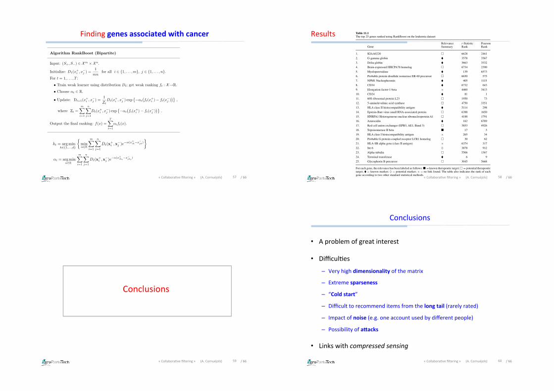
Results
58«CollaboraDvefiltering»(A.Cornuéjols)
“48740_7P_8291_011.tex” — 10/1/2012 — 17:41 — page 368
368 11 Learning to Rank
if the feedback is dense. Nevertheless, even in such cases, we saw how the algorithm canbe implemented very efficiently in the special but natural case of layered or quasi-layeredfeedback. Further, we saw how RankBoost and its variants can be used with weak learn-ing algorithms intended for ordinary binary classification, possibly with confidence-ratedpredictions. Treating multi-label, multiclass classification as a ranking problem leads to theAdaBoost.MR algorithm. Finally, we looked at applications of RankBoost to parsing andfinding cancer-related genes.
Table 11.1The top 25 genes ranked using RankBoost on the leukemia dataset
Relevance t-Statistic PearsonGene Summary Rank Rank
1. KIAA0220 ! 6628 2461
2. G-gamma globin " 3578 3567
3. Delta-globin " 3663 3532
4. Brain-expressed HHCPA78 homolog ! 6734 2390
5. Myeloperoxidase " 139 6573
6. Probable protein disulfide isomerase ER-60 precursor ! 6650 575
7. NPM1 Nucleophosmin " 405 1115
8. CD34 " 6732 643
9. Elongation factor-1-beta × 4460 3413
10. CD24 " 81 1
11. 60S ribosomal protein L23 ! 1950 73
12. 5-aminolevulinic acid synthase ! 4750 3351
13. HLA class II histocompatibility antigen " 5114 298
14. Epstein-Barr virus small RNA-associated protein ! 6388 1650
15. HNRPA1 Heterogeneous nuclear ribonucleoprotein A1 ! 4188 1791
16. Azurocidin " 162 6789
17. Red cell anion exchanger (EPB3, AE1, Band 3) ! 3853 4926
18. Topoisomerase II beta # 17 3
19. HLA class I histocompatibility antigen × 265 34
20. Probable G protein-coupled receptor LCR1 homolog ! 30 62
21. HLA-SB alpha gene (class II antigen) × 6374 317
22. Int-6 ♦ 3878 912
23. Alpha-tubulin ! 5506 1367
24. Terminal transferase " 6 9
25. Glycophorin B precursor ! 3045 5668
For each gene, the relevance has been labeled as follows: # = known therapeutic target; ! = potential therapeutictarget; " = known marker; ♦ = potential marker; × = no link found. The table also indicates the rank of eachgene according to two other standard statistical methods.
/66
Conclusions
59«CollaboraDvefiltering»(A.Cornuéjols) /66
Conclusions
• Aproblemofgreatinterest
• DifficulDes
– Veryhighdimensionalityofthematrix
– Extremesparseness
– “Coldstart”
– Difficulttorecommenditemsfromthelongtail(rarelyrated)
– Impactofnoise(e.g.oneaccountusedbydifferentpeople)
– Possibilityofa9acks
• Linkswithcompressedsensing
60«CollaboraDvefiltering»(A.Cornuéjols)
/66
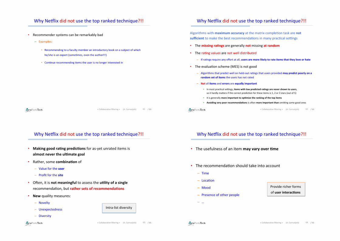
WhyNeflixdidnotusethetoprankedtechnique?!!
• Recommendersystemscanberemarkablybad
– Examples:
• Recommendingtoafacultymemberanintroductorybookonasubjectofwhich
he/sheisanexpert(someDmes,eventheauthor!!!)
• ConDnuerecommendingitemstheuserisnolongerinterestedin
61«CollaboraDvefiltering»(A.Cornuéjols) /66
WhyNeflixdidnotusethetoprankedtechnique?!!
AlgorithmswithmaximumaccuracyatthematrixcompleDontaskarenotsufficienttomakethebestrecommendaDonsinmanypracDcalsexngs
• Themissingra'ngsaregenerallynotmissingatrandom
• TheraDngvaluesarenotwelldistributed
– IfraDngsrequireanyeffortatall,usersaremorelikelytorateitemsthattheyloveorhate
• TheevaluaDonscheme(MES)isnotgood
– Algorithmsthatpredictwellonheld-outraDngsthatusersprovidedmaypredictpoorlyonarandomsetofitemstheusershasnotrated
– Notallitemsanderrorsareequallyimportant
• InmostpracDcalsexngs,itemswithlowpredictedra'ngsarenevershowntousers,soithardlymaGersifthecorrectpredicDonfortheseitemsis1,2or3stars(outof5)
• Itisgenerallymoreimportanttoop'mizetherankingofthetopitems
• Avoidingverypoorrecommenda'onsisosenmoreimportantthanomixngsomegoodones
62«CollaboraDvefiltering»(A.Cornuéjols)
/66
WhyNeflixdidnotusethetoprankedtechnique?!!
• Makinggoodra'ngpredic'onsforas-yetunrateditemsis
almostnevertheul'mategoal
• Rather,somecombina'onof
– Valuefortheuser
– Profitforthesite
• Osen,itisnotmeaningfultoassesstheu'lityofasinglerecommendaDon,butrathersetsofrecommenda'ons
• Newqualitymeasures:
– Novelty
– Unexpectedness
– Diversity
63«CollaboraDvefiltering»(A.Cornuéjols)
Intra-listdiversity
/66
WhyNeflixdidnotusethetoprankedtechnique?!!
• Theusefulnessofanitemmayvaryover'me
• TherecommendaDonshouldtakeintoaccount
– Time
– LocaDon
– Mood
– Presenceofotherpeople
– …
64«CollaboraDvefiltering»(A.Cornuéjols)
Providericherforms
ofuserinterac'ons
/66
OpenquesDons
• HowtocombinecontextinformaDonwithmatrixcompleDonapproaches?
• Howtofindthemost“informa've”itemsthatusersshouldbeaskedtorate?
• HowtodesignalgorithmsthatbalancediversityandaccuracyinanopDmal
way?
• ArecommendersystemisosenonlyonecomponentwithinaninteracDveapplicaDon.Howtointegrateallcomponents?
65«CollaboraDvefiltering»(A.Cornuéjols)
The current research community is too focused on
abstract performance metrics which do take into
accountallrelevantaspectsoftheproblem
/66
References
S.Agarwal&S.Senguptat
Rankinggenesbyrelevancetodisease
8thAnnualInt.Conf.onComputaDonalSystemsBioinformaDcs,2009
A.Cornuéjols&L.Miclet
ApprenDssageArDficiel.Conceptsetalgorithmes
Eyrolles(2°éd.),2010
D.Jannach,P.Resnick,A.Tuzhilin&M.Zanker
RecommenderSystems–BeyondmatrixcompleDon
Comm.oftheACM,Nov.2016,Vol.59,No.11
66«CollaboraDvefiltering»(A.Cornuéjols)