AFRL-OSR-VA-TR-2015-0177

Collaborative Research Model Reduction for Nonlinear and Parametric Systems with Uncertainty

Matthias HeinkenschlossWILLIAM MARSH RICE UNIV HOUSTON TX

07/14/2015Final Report

DISTRIBUTION A: Distribution approved for public release.

Air Force Research LaboratoryAF Office Of Scientific Research (AFOSR)/RTA

Arlington, Virginia 22203Air Force Materiel Command

Page 1 of 1

7/17/2015https://livelink.ebs.afrl.af.mil/livelink/llisapi.dll

REPORT DOCUMENTATION PAGE Form Approved OMB No. 0704-0188

The public reporting burden for this collection of information is estimated to average 1 hour per response, including the time for reviewing instructions, searching existing data sources, gathering and maintaining the data needed, and completing and reviewing the collection of information. Send comments regarding this burden estimate or any other aspect of this collection of information, including suggestions for reducing the burden, to the Department of Defense, Executive Service Directorate (0704-0188). Respondents should be aware that notwithstanding any other provision of law, no

person shall be subject to any penalty for failing to comply with a collection of information if it does not display a currently valid OMB control number.

PLEASE DO NOT RETURN YOUR FORM TO THE ABOVE ORGANIZATION.

1. REPORT DATE (DD-MM-YYYY)

10-07-2015 2. REPORT TYPE

Final Report 3. DATES COVERED (From - To)

15-April-2012 to 14-April-2015

4. TITLE AND SUBTITLE

COLLABORATIVE RESEARCH: MODEL REDUCTION FOR NONLINEAR AND

PARAMETRIC SYSTEMS WITH UNCERTAINTY

5a. CONTRACT NUMBER

5b. GRANT NUMBER

FA9550-12-1-0155

5c. PROGRAM ELEMENT NUMBER

6. AUTHOR(S)

Heinkenschloss, Matthias

Sorensen, Danny, C.

5d. PROJECT NUMBER

5e. TASK NUMBER

5f. WORK UNIT NUMBER

7. PERFORMING ORGANIZATION NAME(S) AND ADDRESS(ES)

Department of Computational and Applied Mathematics - MS 134

William Marsh Rice University

6100 Main Street

Houston, Texas 77005

8. PERFORMING ORGANIZATIONREPORT NUMBER

9. SPONSORING/MONITORING AGENCY NAME(S) AND ADDRESS(ES)

USAF, AFRL

AF Office of Scientific Research

875 N. Randolph Street

Arlington, VA 22203

10. SPONSOR/MONITOR'S ACRONYM(S)

11. SPONSOR/MONITOR'S REPORTNUMBER(S)

12. DISTRIBUTION/AVAILABILITY STATEMENT

Public Release distribution A

13. SUPPLEMENTARY NOTES

14. ABSTRACT

This project has developed and analyzed new mathematical algorithms to substantially reduce the complexity of simulating and optimizing

parametrically dependent systems and to support decision-making under uncertainty. Specifically, this research has advanced the state of the art in

reduced order modeling based on projections and on the discrete empirical interpolation method (DEIM) for nonlinear systems, developed new

adaptive sampling methods for optimization of systems with uncertain inputs, devised a domain decomposition based methods to systematically

integrate the uncertainty propagation through components into uncertainty propagation through a systems composed of these components,

established a so-called CUR factorization based on the DEIM that provides a low rank approximate factorization of a given large matrix with

applications to POD model reduction and analysis of data. The feasibility of our algorithms was demonstrated on a number of problems with

relevance to the Air Force.

15. SUBJECT TERMS

16. SECURITY CLASSIFICATION OF: 17. LIMITATION OFABSTRACT

UU

18. NUMBEROFPAGES

19a. NAME OF RESPONSIBLE PERSON

Melinda Cotten a. REPORT

U

b. ABSTRACT

U

c. THIS PAGE

U 19b. TELEPHONE NUMBER (Include area code)

713-348-6200

Standard Form 298 (Rev. 8/98) Prescribed by ANSI Std. Z39.18

Adobe Professional 7.0

Reset

INSTRUCTIONS FOR COMPLETING SF 298

1. REPORT DATE. Full publication date, including

day, month, if available. Must cite at least the year and

be Year 2000 compliant, e.g. 30-06-1998; xx-06-1998;

xx-xx-1998.

2. REPORT TYPE. State the type of report, such as

final, technical, interim, memorandum, master's thesis,

progress, quarterly, research, special, group study, etc.

3. DATES COVERED. Indicate the time during which

the work was performed and the report was written,

e.g., Jun 1997 - Jun 1998; 1-10 Jun 1996; May - Nov

1998; Nov 1998.

4. TITLE. Enter title and subtitle with volume number

and part number, if applicable. On classified

documents, enter the title classification in parentheses.

5a. CONTRACT NUMBER. Enter all contract numbers

as they appear in the report, e.g. F33615-86-C-5169.

5b. GRANT NUMBER. Enter all grant numbers as

they appear in the report, e.g. AFOSR-82-1234.

5c. PROGRAM ELEMENT NUMBER. Enter all

program element numbers as they appear in the report,

e.g. 61101A.

5d. PROJECT NUMBER. Enter all project numbers as

they appear in the report, e.g. 1F665702D1257; ILIR.

5e. TASK NUMBER. Enter all task numbers as they

appear in the report, e.g. 05; RF0330201; T4112.

5f. WORK UNIT NUMBER. Enter all work unit

numbers as they appear in the report, e.g. 001;

AFAPL30480105.

6. AUTHOR(S). Enter name(s) of person(s)

responsible for writing the report, performing the

research, or credited with the content of the report. The

form of entry is the last name, first name, middle initial,

and additional qualifiers separated by commas, e.g.

Smith, Richard, J, Jr.

7. PERFORMING ORGANIZATION NAME(S) AND

ADDRESS(ES). Self-explanatory.

8. PERFORMING ORGANIZATION REPORT NUMBER.

Enter all unique alphanumeric report numbers assigned by

the performing organization, e.g. BRL-1234;

AFWL-TR-85-4017-Vol-21-PT-2.

9. SPONSORING/MONITORING AGENCY NAME(S)

AND ADDRESS(ES). Enter the name and address of the

organization(s) financially responsible for and monitoring

the work.

10. SPONSOR/MONITOR'S ACRONYM(S). Enter, if

available, e.g. BRL, ARDEC, NADC.

11. SPONSOR/MONITOR'S REPORT NUMBER(S).

Enter report number as assigned by the sponsoring/

monitoring agency, if available, e.g. BRL-TR-829; -215.

12. DISTRIBUTION/AVAILABILITY STATEMENT. Use

agency-mandated availability statements to indicate the

public availability or distribution limitations of the report. If

additional limitations/ restrictions or special markings are

indicated, follow agency authorization procedures, e.g.

RD/FRD, PROPIN, ITAR, etc. Include copyright

information.

13. SUPPLEMENTARY NOTES. Enter information not

included elsewhere such as: prepared in cooperation

with; translation of; report supersedes; old edition number,

etc.

14. ABSTRACT. A brief (approximately 200 words)

factual summary of the most significant information.

15. SUBJECT TERMS. Key words or phrases identifying

major concepts in the report.

16. SECURITY CLASSIFICATION. Enter security

classification in accordance with security classification

regulations, e.g. U, C, S, etc. If this form contains

classified information, stamp classification level on the top

and bottom of this page.

17. LIMITATION OF ABSTRACT. This block must be

completed to assign a distribution limitation to the abstract.

Enter UU (Unclassified Unlimited) or SAR (Same as

Report). An entry in this block is necessary if the abstract

is to be limited.

Standard Form 298 Back (Rev. 8/98)

COLLABORATIVE RESEARCH: MODEL REDUCTION FOR NONLINEAR ANDPARAMETRIC SYSTEMS WITH UNCERTAINTY

FA9550-12-1-0155 and FA9550-12-1-0420

Matthias Heinkenschloss and Danny C. SorensenDepartment of Computational and Applied Mathematics

Rice University, Houston, Texas

Karen WillcoxDepartment of Aeronautics & Astronautics

Massachusetts Institute of Technology

Abstract

This project has developed and analyzed new mathematical algorithms to substantially reducethe complexity of simulating and optimizing parametrically dependent systems and to supportdecision-making under uncertainty. Specifically, this research has advanced the state of the art inreduced order modeling based on projections and on the discrete empirical interpolation method(DEIM) for nonlinear systems, developed new adaptive sampling methods for optimization ofsystems with uncertain inputs, devised a domain decomposition based methods to systematicallyintegrate the uncertainty propagation through components into uncertainty propagation through asystems composed of these components, established a so-called CUR factorization based on theDEIM that provides a low rank approximate factorization of a given large matrix with applicationsto POD model reduction and analysis of data. The feasibility of our algorithms was demonstratedon a number of problems with relevance to the AirForce.

1 Introduction

Effective computational tools to support decision-making under uncertainty have become essentialin the design and operation of aerospace systems. Many problems of relevance to the Air Force aredescribed by mathematical models of high complexity—involving multiple disciplines, character-ized by a large number of parameters, and impacted by multiple sources of uncertainty. The accu-rate and efficient propagation of uncertainties in parameters through these complex, high fidelitycomputational models is a significant challenge. This project has developed new mathematicalalgorithms and analyses to substantially reduce the complexity of simulating and optimizing para-metrically dependent systems and of propagating uncertainty through systems. In particular, thisresearch has advanced the state of the art in reduced order modeling based on projections and onthe discrete empirical interpolation method (DEIM) for nonlinear systems, developed new adaptivesampling methods for optimization of systems with uncertain inputs, devised a domain decompo-sition based methods to systematically integrate the uncertainty propagation through componentsinto uncertainty propagation through a systems composed of these components, established a so-

1

called CUR factorization based on the DEIM that provides a low rank approximate factorizationof a given large matrix with applications to POD model reduction and analysis of data. The fea-sibility of algorithms was demonstrated on a number of problems with relevance to the AirForce.This report highlights several of our research results. More details can be found in the publications[1, 2, 3, 4, 5, 7, 8, 9, 10, 11, 13] and theses [6, 12] that resulted from this research.

Sections 2.1 to 2.4 summarize our advancements to the state of the art in reduced order modelingbased on projections and on the discrete empirical interpolation method (DEIM) for nonlinear sys-tems. Section 2.1 is concerned with the application of the Discrete Empirical Interpolation Method(DEIM) to systems obtained by finite element discretizations of partial differential equations, andto a class of parameterized system that arises, e.g., in shape optimization. Careful analysis andreorganizations of computations lead to evaluations of the DEIM reduced order models (ROMs)that are substantially faster than those of the standard projection based ROMs. Additional gainsare obtained with the DEIM ROMs when one has to compute derivatives of the model with respectto the parameter.

Traditionally, projection based reduced order models use only one subspace for all parameters.To obtain an accurate ROM, this can require relatively large dimensional subspaces, and, conse-quently, result in a less efficient ROM. The approach in Section 2.2 divides the parameter spaceinto regions and for each region develops a different ROM. The regions in parameter space are de-termined using machine learning methods in the offline computational phase via clustering. Thisapproach can lead to significantly smaller and therefore computationally cheaper ROMs.

Section 2.3 summarizes our development of an efficient approach for a-posteriori error estimationfor POD-DEIM reduced nonlinear dynamical systems. Our a-posteriori error estimator can beefficiently decomposed in an offline/online fashion and is obtained by a one dimensional auxiliaryODE during reduced simulations.

The application of the DEIM requires that a component of the system nonlinearity depends onlyon a few components of the vector of arguments, and it requires explicit knowledge of this depen-dence. If DEIM based model reduction is applied to existing codes, determining this dependencycan be tedious and error prone task. Section 2.4 describes how standard techniques of automaticdifferentiation (AD) can be adapted to producing such a code and hence can facilitate the use ofDEIM by non-experts.

The methods in sections 2.5 and 2.6 are concerned with efficient uncertainty propagation throughcoupled systems, and efficient optimization of PDE systems with uncertain parameters. Thus,while the methods summarized in sections 2.1 to 2.4 deal with complexity reduction in simulationof general parameterized systems, the approaches in sections 2.5 and 2.6 integrate the statisticaldistributions of the uncertain parameters.

We have developed a rigorous framework based on trust-region algorithms and adaptive stochasticcollocation for the efficient solution of optimization problems governed by partial differential equa-tions with uncertain parameters. Sparse grid collocation or other sampling methods lead to inexact

2

objective functions and gradients in the optimization problems. Our new trust-region frameworkrigorously manages the use of this inexact problem information. As a result, we dramatically re-duce the number of samples required, which leads to a dramatic reduction in the computationalcost. Moreover, numerical results indicate that our new algorithm rapidly identifies the stochas-tic variables that are relevant to obtaining an accurate optimal solution. When the number ofsuch variables is independent of the dimension of the stochastic space, the algorithm exhibits neardimension-independent behavior.

Decomposition of a system into subsystems or component parts is another strategy to managecomplexity. We have developed a domain decomposition approach for uncertainty analysis. Ourapproach sketched in Section 2.6 generates computational models for the propagation of uncer-tainty through the subsystems. These subsystem models are computed independently in an “of-fline” phase and they account for propagation of uncertainly through interface conditions, whichis important for the coupled systems. Once the subdomain models are constructed, importancesampling is used to couple the subdomain models and analyze the propagation of uncertainty inthe global system. This last step is performed in an“online” phase and does not require expensivesimulations.

Finally, Section 2.7 summarizes our development and analyzes of a new CUR matrix factorizationfor matrices built from large-scale data sets. The CUR offers two advantages over the SVD: whenthe data in A are sparse, so too are the C and R matrices, unlike the matrices of singular vectors;and the columns and rows that comprise C and R are representative of the data (e.g., sparse,nonnegative, integer valued, etc.). Our algorithm is novel in that it only requires one pass throughthe data A and only requires a few columns of A to be in memory at any given step of the algorithm.This is ideal for POD based model reduction schemes since the high dimensional trajectory neednot be stored.

2 Accomplishments

This rsection highlights several of our research results. More details can be found in the publica-tions [1, 2, 3, 4, 5, 7, 8, 9, 10, 11, 13] and theses [6, 12] that resulted from this research.

2.1 Application of the Discrete Empirical Interpolation Method to ReducedOrder Modeling of Nonlinear and Parametric Systems

Projection based methods lead to reduced order models (ROMs) with dramatically reduced num-bers of equations and unknowns. However, for nonlinear or parametrically varying problems thecost of evaluating these ROMs still depends on the size of the full order model and therefore isstill expensive. The Discrete Empirical Interpolation Method (DEIM) further approximates the

3

nonlinearity in the projection based ROM. The resulting DEIM ROM nonlinearity depends onlyon a few components of the original nonlinearity. If each component of the original nonlinearitydepends only on a few components of the argument, the resulting DEIM ROM can be evaluatedefficiently at a cost that is independent of the size of the original problem. For systems obtainedfrom finite difference approximations, the ith component of the original nonlinearity often dependsonly on the ith component of the argument. This is different for systems obtained using finite ele-ment methods, where the dependence is determined by the mesh and by the polynomial degree ofthe finite element subspaces. Our paper [AHS13] describes two approaches of applying DEIM inthe finite element context, one applied to the assembled and the other to the unassembled form ofthe nonlinearity. We carefully examine how the DEIM is applied in each case, and the substantialefficiency gains obtained by the DEIM. In addition, we demonstrate how to apply DEIM to obtainROMs for a class of parameterized system that arises, e.g., in shape optimization. The evaluationsof the DEIM ROMs are substantially faster than those of the standard projection based ROMs.Additional gains are obtained with the DEIM ROMs when one has to compute derivatives of themodel with respect to the parameter.

The following example is a semillinear elliptic reaction-advection-diffusion partial differentialequation (PDE) posed on Ω = (0,18)× (0,9)× (0,9). A concentration of u = 0.2 is imposedon 0× [3,6]××[3,6]. We want to represent the concentration (the solution of the semillinearelliptic PDE) for varying parameter (ln(A),E) in the reaction term. A finite element mesh (Mesh 2)of the domain Ω and concentration corresponding to parameter (ln(A),E) = (6.4,0.11) are shownin Figure 1.

Figure 1: Coarse finite element mesh of the domain Ω (left plot) and solution of the semillinearreaction-advection-diffusion PDE with parameter (ln(A),E) = (6.4,0.11) (right plot).

4

piecewise linear FEMassembled unassembled

Figure 2: The tetrahedra that contain DEIM points for piecewise linear finite elements are shown.

Figure 2 shows the tetrahedra in Mesh 2 that contain a node corresponding to a DEIM point. Theplots in the left column correspond to the DEIM applied to the assembled form of the nonlinearity.The expense of evaluating the DEIM reduced order model is proportional to the number of nodesthe DEIM indices are connected to. Figure 2 already indicates that the unassembled form of DEIMis more efficient. This is confirmed by the timing results in Table 1. Table 1 clearly show thetime saving of DEIM-POD receded order models over naive POD reduced order model for bothpiecewise linear (p = 1) and piecewise quadratic (p = 2) finite elements. Using the unassembledform of DEIM leads to additional gains.

Polynomial degree p = 1 p = 2Mesh number 1 2 3 1 2Full 1.78 (4) 10.60 (3) 43.30 (3) 7.80 (3) 185.00 (3)POD 1.28 (4) 8.04 (3) 23.80 (3) 4.12 (3) 38.80 (3)POD-DEIM 0.15 (4) 0.10 (3) 0.21 (4) 0.21 (3) 0.40 (3)POD-DEIM-u 0.16 (9) 0.07 (4) 0.10 (4) 0.01 (4) 0.18 (4)

Table 1: The computing times (in sec) and the number of Newton iterations (in parenthesis) neededto solve the full order model, the POD reduced order model, the POD-DEIM reduced order model,and the POD-DEIM-u (unassembled) reduced order model for different grid levels and linear (p =1) and quadratic (p = 2) finite elements.

2.2 Localized DEIM

We have proposed the Localized DEIM (LDEIM) as way to improve the efficiency of DEIM ROMsfor nonlinear parameterized PDEs [PBWB13]. Whereas DEIM projects the nonlinear term onto

5

one global subspace, our LDEIM method computes k local subspaces, each tailored to a particu-lar region of characteristic system behavior. Then, depending on the current state of the system,LDEIM selects an appropriate local subspace for the approximation of the nonlinear term. In thisway, the dimensions of the local DEIM subspaces, and thus the computational costs, remain loweven though the system might exhibit a wide range of behaviors as it passes through differentregimes. LDEIM uses machine learning methods in the offline computational phase to discoverthese regions via clustering. In our implementation, the snapshots are clustered with k-means. Lo-cal DEIM approximations are then computed for each cluster. In the online computational phase,machine-learning-based classification procedures select one of these local subspaces adaptively asthe computation proceeds. We use a nearest neighbor classifier. The classification can be achievedusing either the system parameters or a low-dimensional representation of the current state of thesystem obtained via feature extraction.

The LDEIM approach is demonstrated for a reacting flow example of a premixed H2-Air flame.The physics are modeled with the one-step reaction mechanism

2H2 +O2→ 2H2O ,

where H2 is the fuel, O2 is the oxidizer, and H2O is the product. The evolution of the flame in thedomain Ω is given by the nonlinear advection-diffusion-reaction equation

κ∆y−w∇y+ f(y,µ) = 0 , (1)

where y = [yH2,yO2,yH2O,T ]T contains the mass fractions of species H2,O2, and H2O and thetemperature. The constants κ = 2.0cm2/sec and w = 50cm/sec are the molecular diffusivity andthe velocity of the velocity field in x1 direction, respectively. The geometry of the problem is shownin Figure 3. We prescribe homogeneous Dirichlet boundary conditions on the mass fractions on Γ1and Γ3, and homogeneous Neumann conditions on temperature and mass fractions on Γ4,Γ5, andΓ6. We have Dirichlet conditions on Γ2 with yH2 = 0.0282,yO2 = 0.2259,yH2O = 0,yT = 950K,and on Γ1,Γ3 with yT = 300K.

Γ4

Γ5

Γ6

Γ1

Γ2

Γ3

Ω

3cm

3cm

3cm

Fuel

+

Oxidizer

x2

x1

18cm

9cm

Figure 3: The spatial domain of the reacting flow simulation.

The nonlinear reaction source term f(y,µ = [ fH2(y,µ), fO2(y,µ), fH2O(y,µ), fT (y,µ)]T in (1) has

6

the components

fi(y,µ) = −νi (ηH2yH2)2 (ηO2yO2)µ1 exp

(− µ2

RT

), i = H2,O2,H2O

fT (y,µ) = Q fH2O(y,µ),

where νi and ηi are constant parameters, R = 8.314472J/(mol K) is the universal gas constant, andQ= 9800K is the heat of reaction. The parameters µ= (µ1,µ2)∈D with D = [5.5e+11,1.5e+03]×[1.5e+13,9.5e+03] are the pre-exponential factor and the activation energy, respectively. The equa-tion (1) is discretized using the finite difference method on a 73×37 grid leading to N = 10,804degrees of freedom. The resulting nonlinear system of equations is solved with the Newton method.The snapshots are computed for the parameters on a 50×50 equidistant grid in D .

Figure 4 compares DEIM, parameter-based LDEIM with splitting and clustering, and state-basedLDEIM. For splitting, we set the tolerance ε to 1e-08, which is about two orders below what DEIMachieves. For the parameter-based LDEIM with clustering, the number of clusters is set to 5. Moreclusters lead to an unstable behavior. For the state-based LDEIM, however, we set the number ofclusters to 15. The state-based LDEIM uses a point-based feature extraction with M = 5 dimen-sions. In all cases, we have 40 POD modes. In Figure 4, we see that the results of the parameter-based LDEIM with clustering do not improve after about 10 DEIM modes. Again, the clusteringbecomes unstable. However, this is not the case for state-based LDEIM which achieves about twoorders of magnitude better accuracy than DEIM. The same holds for the splitting approach.

Figure 4: For the reacting flow example, the comparison between DEIM, parameter-based LDEIM,and state-based LDEIM. The results are shown for 40 POD and 20 DEIM modes. State-basedLDEIM achieves about two orders of magnitude better accuracy than DEIM for the same numberof DEIM modes.

7

2.3 A-Posteriori Error Estimation for DEIM

We have introduced an efficient approach for a-posteriori error estimation for POD-DEIM reducednonlinear dynamical systems [WSH12]. The considered nonlinear systems may also include timeand parameter-affine linear terms as well as parametrically dependent inputs and outputs. The re-duction process involves a Galerkin projection of the full system and approximation of the system’snonlinearity by the DEIM method [Chaturantabut & Sorensen (2010)]. The proposed a-posteriorierror estimator can be efficiently decomposed in an offline/online fashion and is obtained by a onedimensional auxiliary ODE during reduced simulations. Key elements for efficient online compu-tation are partial similarity transformations and matrix DEIM approximations of the nonlinearityJacobians. The theoretical results are illustrated by application to an unsteady Burgers equationand a cell apoptosis model.

The key ideas of our error estimation procedure is an application of a Gronwall-like differentialinequality for the error norm ‖y(t)−yr(t)‖ (full vs. reduced state) , estimation of local logarithmicLipschitz constants and an estimation of the DEIM approximation error for a ROM of order musing a higher order DEIM approximation of order m+m′. Essentially, we treat the higher orderapproximation heuristically as representing the true state. We use these tools to provide a-posteriorierror bounds which can be computed along with the reduced system trajectory at negligible cost.Only a simple 1D ODE must be propagated along with the reduced state calculation.

5 10 15 20 25 30

3.2e−002

1.0e−001

3.2e−001

1.0e+000

3.2e+000

Linf−L2 absolute error

order

5

10

15

20

25

305

1015

2025

3035

40

3.2e−002

1.0e−001

3.2e−001

1.0e+000

3.2e+000

error order

Estimated absolute error

order

Figure 5: (Left) Absolute error of DEIM Approximation (Right) Demonstration of Error Estimatefor varying m and m′

The graphs in Figure 6 illustrate the effectiveness of our error estimator. The graph on the leftshows the absolute error of the reduced state from the DEIM reduced model with the true state.The right graph is a surface plot showing the error estimate using the m+m′ model in place of thetrue state. The axis labeled “order” shows the error as the model order m is increased. The axislabeled “error order” shows the estimated error as m′ increases. The fact that the surface quicklyflattens out in the m′ direction verifies that m′ does not need to be large, it typically adequate for

8

accurate error estimation at values between 5 and 10. This plot is for a 1D Burgers’ equation butwe obtained virtually identical behavior for a 60,000 variable 2D Reaction-Diffusion model CellApoptosis.

2.4 Automating DEIM

As mentioned previously, the Discrete Empirical Interpolation Method (DEIM) is based upon amodification to proper orthogonal decomposition which is designed to reduce the computationalcomplexity for evaluating the reduced order nonlinear term. The DEIM approach is based upon aninterpolatory projection and only requires evaluation of a few selected components of the originalnonlinear term. Thus, implementation of the reduced order nonlinear term requires a new code tobe derived from the original code for evaluating the nonlinearity. We have developed a methodol-ogy for automatically deriving a code for the reduced order nonlinearity directly from the originalnonlinear code. The methodology is an adaptation of standard techniques of automatic differenti-ation (AD). This capability removes the possibly tedious and error prone task of producing such acode by hand and hence can facilitate the use of DEIM by non-experts.

We have a working prototype system that establishes proof of concept [CS12]. We were ableto automatically produce a reduced order code from the original code for 2-phase miscible flowsimulation. This automatically derived code was able to completely reproduce the simulationresults from the hand coded ROM with essentially no degradation in computation time. The ideais to first obtain a computational graph representation of the original code and then this graph is“pruned” to retain only the graph necessary to compute the code to evaluate the DEIM selectednodes (which correspond to the DEIM indices of the desired components of the nonlinearity). Thepruned graph is then used in a reverse process to generate the code for the ROM. Using standardAD techniques, one could also generate the Jacobian of the ROM automatically.

2.5 Trust-Region Algorithms with Adaptive Stochastic Collocation for PDEOptimization under Uncertainty.

We have improved our trust-region adaptive sparse grid framework for the solution of optimizationproblems governed by partial differential equations (PDEs) with random coefficients. While previ-ously adaptive sparse grids were only used to generate the models used to commute the step insidethe trust-region framework [7], we now also allow the approximation of function values usingadaptive sparse grids [8]. This results in substantial computational savings. With our algorithmicimprovements, numerical solutions that previously required high performance parallel computers1

can now be run on a desktop [8].1The computations in [7] were carried out on RedSky, an institutional computing cluster at Sandia National Labo-

ratories. The cluster is built on a 3D toroidal QDR InfiniBand interconnect and provides 2,816 compute nodes, eachwith 8 cores, 2.93 GHz Nehalem X5570 processors, and 12 GB RAM per compute node.

9

The numerical solution of optimization problems governed by PDEs with random coefficients po-tentially requires a the large number of deterministic PDE solves at each optimization iteration.Our algorithm for solving such problems based on a combination of adaptive sparse-grid collo-cation for the discretization of the PDE in the stochastic space and a trust-region framework foroptimization and fidelity management of the stochastic discretization. The overall algorithm adaptsthe collocation points based on the progress of the optimization algorithm and the impact of therandom variables on the solution of the optimization problem. It frequently uses few collocationpoints initially and increases the number of collocation points only as necessary, thereby keepingthe number of deterministic PDE solves low while guaranteeing convergence. Our trust-regionframework now allows adaptation to build the model, as well as to approximate the objective func-tion [8]. Our trust-region framework can be used in a wide range of applications, and extends thestate-of-the-art in trust region methods for problems with inexact function and derivative infor-mation. Currently an error indicator is used to estimate gradient errors due to adaptive stochasticcollocation, but other adaptive discretizations could be used as well.

The following example is motivated by the optimal control of direct field acoustic testing (DFAT).An important objective in DFAT is to accurately shape sound pressure fields in a region of interestby using acoustic sources, such as loudspeakers, located away from and directed at the region ofinterest. When the refractive index of the medium in the region of interest is random, we mayassume that the governing physics are modeled by the stochastic Helmholtz equation

−∆u(y,x)− k2(1+σε(y,x))2u(y,x) = z(x) ∀ (y,x) ∈ Γ×D (2)

with Robin boundary conditions ∂

∂nu(y,x) = iku(y,x) for all (y,x) ∈ Γ× ∂D. Here x is the spatialvariable in the spatial domain D and y is the random variable. We consider an idealized DFATexample in two spatial dimensions, where the domain is D = (−5,5)2. The goal of this controlproblem is to match the wave pressure u to a desired wave pressure w ∈ L2(D;C) in the diskDR = x ∈ D : ‖x‖2 ≤ R ⊂ D. We apply distributed controls in DC, which is the union of theregions occupied by 20 loudspeakers arranged in a circle exterior to DR. Figure 6 depicts theexperimental setup.

10

DR

Figure 6: Left: A sketch of the computational domain with the region of interest DR and 20 loud-speakers spaced uniformly along a circle surrounding DR. The red (lighter) color denotes uncer-tainty in the refraction index inside DR and uncertainty in the loudspeaker enclosures (includingthickness and sound speed). The blue (darker) color stands for the loudspeaker control regions,whose union is denoted by DC. Right: The real component of the desired state, w.

In this example we study three sources of uncertainty: refractive index, loudspeaker thickness,and speed of sound in each loudspeaker. We assume that the stochastic refractive index is of theform ε(y,x) =∑

Mm=1 εm(x)ym and that its covariance is given by a Matern covariance functions. The

series representation of ε is motivated by a truncated Karhunen-Loeve (KL) expansion. In total, wehave dim = 40+M random variables, 40 random loudspeaker parameters (enclosure thicknessesand wave number for each speaker) and M random variables representing the stochastic refractiveindex ε. For additional details see Section 5.2 in [KHRW14]. Figure 7 shows the optimal solutionfor (dim = 60 random variables (i.e., M = 20).

Figure 7: Left: The real parts of the computed optimal controls. Center: The real part of theexpected value of the optimal state, restricted to the region of interest. Right: The real part of thestandard deviation of the optimal state.

11

Table 2 gives the computational cost of our algorithm as the stochastic dimension increases fromdim = 42 to dim = 80 and it illustrates the power of our algorithm. Even for the largest dimension,dim= 80, the problem can now be solved using a desktop. In contrast, the 40-dimensional problemusing the previous version of our algorithm [KHRW13] required 1,804,001 collocation pointsfor the evaluation of the high-fidelity objective function, while the 80-dimensional problem nowrequires only 311 points due to the adaptive objective function evaluations. We also note that in thisexample many of the random variables are not important for the optimization context. However,it is not clear which one are the important ones. Our algorithm is able to automatically detect theimportant random variables and automatically zooms in on approximately 10 (out of 80) stochasticdimensions that are relevant to achieving objective function and gradient consistency conditionsrequired by the trust-region framework. As a result it vastly reduces the effective problem sizeand, in this example, shows a convergence behavior that is nearly independent of the stochasticdimension.

dim PDE Solves CPobj CPgrad Obj. Value42 11,543 145 145 5.254244 32,739 233 481 5.263746 60,617 243 1,453 5.264148 79,221 247 2,961 5.264150 90,157 251 4,569 5.264160 100,911 271 7,621 5.264170 103,979 291 8,233 5.264180 105,607 311 8,253 5.2641

Table 2: Computational cost of the fully adaptive trust-region algorithm applied to the Helmholtzcontrol example. Here dim is the stochastic dimension, PDE Solves is the total number of forwardand adjoint PDE solves, CPobj is the final number of collocation points used by the adaptiveobjective function scheme, CPgrad is the final number of collocation points used by the adaptivesubproblem (gradient) model, and Obj. Value is the computed value of the objective function attermination.

2.6 A Domain-Decomposition Approach for Uncertainty Analysis.

We have proposed a new decomposition approach for uncertainty analysis of systems governedby PDEs [LW14]. The system is split into local components using domain decomposition. Ourdomain-decomposed uncertainty quantification (DDUQ) approach performs uncertainty analysisindependently on each local component in an “offline” phase, and then assembles global uncer-tainty analysis results using pre-computed local information in an “online” phase. At the heart ofthe DDUQ approach is importance sampling, which weights the pre-computed local PDE solutionsappropriately so as to satisfy the domain decomposition coupling conditions. To avoid global PDEsolves in the online phase, a proper orthogonal decomposition reduced model provides an efficientapproximate representation of the coupling functions.

12

The DDUQ approach comprises the following three steps: (1) pre-step: generate POD basis forinterface functions; (2) offline step: generate local solution samples and construct surrogates forthe coupling functions; (3) online step: estimate target input PDFs using surrogates and re-weightoutput samples. The pre-step is cheap, since although it performs standard domain decompositioniterations, the number of input samples is small. In the offline stage, expensive computational tasksare fully decomposed into subdomains, i.e., there is no data exchange between subdomains. Theonline stage is relatively cheap, since no PDE solve is required. This approach is summarized inFigure 8, where communication refers to data exchange between subdomains.

DOMAIN DECOMPOSED UNCERTAINTY QUANTIFICATION 11

density estimation, which has a computational cost that scales linearly with the sample sizewhen using efficient density estimation techniques [36, 63]. However, in the numerical studiesof this paper, we use the traditional KDE as implemented in the MATLAB KDE toolbox [32]with cost quadratically dependent on the sample size. This full approach is also summarizedin Figure 6.1, where communication refers to data exchange between subdomains.

Pre-step (cheap)• Generate interface POD basis.(Solve PDEs, has communication, but a few samples)

Offline step for D1 (expensive)• Generate local solution samples.• Construct coupling surrogates.(Solve PDEs, no communication)

Offline step for DM (expensive)• Generate local solution samples.• Construct coupling surrogates.(Solve PDEs, no communication)

q q q

Online step (cheap)• Estimate target input PDFs using coupling surrogates.• Re-weight offline output samples.(No PDE solve, has communication)

HHHHHHHHj?

HHHHHHHHj

?

Fig. 6.1. DDUQ summary.

For the problems of interest (systems governed by PDEs), the cost of the DDUQ ap-proach is dominated by the local PDE solves in the offline step. We perform a rough orderof magnitude analysis of the computational costs by taking the cost of each local PDE solveto be Csolve (i.e., the costs of all local PDE solves are assumed equal for simplicity). Thedominant cost of DDUQ is the total number of local PDE solves,

∑Mi=1 NiCsolve. If we assume

that the offline sample sizes are equal for each subdomain, Ni = Noff for all subdomains i,then this cost can be written as MNoffCsolve.

For comparison, we consider the corresponding cost of system-level Monte Carlo com-bined with parallel domain decomposition for N samples. To simplify the analysis, assumethat KDD domain decomposition iterations are performed for each PDE solve. In prac-tice, the number of domain decomposition iterations may vary from case to case, but theywill typically be of similar magnitude. The cost of the system-level Monte Carlo is thenKDDMNCsolve.

For the same number of samples, N = Noff , the cost of the system-level Monte Carlo isa factor of KDD times larger than the DDUQ cost. This is because the system-level MonteCarlo solves local PDEs at every domain decomposition iteration step. In contrast, DDUQonly solves the local PDEs once at each sample point in the offline step, and uses cheapsurrogates to perform the domain decomposition iterations in the online step. We note thatthe system-level Monte Carlo could also be made more efficient by combining surrogatemodels with parallel domain decomposition, but this situation is not considered in this paper.However, it is important to note that this comparison does not tell the full story of the relative

Figure 8: Domain-decomposed uncertainty quantification (DDUQ) summary.

In the offline stage of DDUQ, we first specify a proposal input PDF from which the samples willbe drawn. We denote the proposal input PDF by pξi,τi(ξi,τi), where ξi is the vector of uncertainparameters corresponding to subdomain i and τi is the vector of interface parameters for subdomaini. The proposal input PDF must be chosen so that its support is large enough to cover the supportof the true (unknown) interface parameters. Provided this condition on the support is met, anyproposal input PDF can be used; however, the better the proposal (in the sense that it generatessufficient samples over the support of the target input PDF) the better the performance of theimportance sampling. A poor choice of proposal input PDF will lead to many wasted samples (i.e.,requiring many local PDE solves).

The next step, still in the offline phase, is to perform uncertainty quantification on each localsubdomain i independently. This involves generating a large number Ni of samples (ξ(s)i ,τ

(s)i )Ni

s=1of pξi,τi(ξi,τi), where the superscript (s) denotes the sth sample, and computing the local solutions

u(x,ξ(s)i ,τ(s)i ) by solving the deterministic problem for each sample. Once the local solutions are

13

computed, we evaluate the local outputs of interest yi(u(x,ξ(s)i ,τ

(s)i )) and store them.

In the online stage of DDUQ, we first generate Non samples, ξ(s)Nons=1, of the joint PDF of inputs

πξ(ξ). For each sample ξ(s), we use the domain decomposition iteration to evaluate the corre-sponding interface parameters. After the above process, we have obtained a set of samples drawnfrom each local target input PDF πξi,τi(ξi,τi). We next estimate each local target input PDF fromthe samples using a density estimation technique, such as kernel density estimation (KDE).

The final step of the DDUQ online stage is to use importance sampling to re-weight the outputsyi

(u(

x,ξ(s)i ,τ(s)i

))Ni

s=1that we generated by PDE solves in the offline stage. The weights, w(s)

i ,are computed by taking the ratio of the estimated target PDF to the proposal PDF for each localsubdomain:

w(s)i =

πξi,τi

(ξ(s)i ,τ

(s)i

)pξi,τi

(ξ(s)i ,τ

(s)i

) , s = 1, . . . ,Ni, i = 1, . . . ,M.

We can show that the probability computed from these weighted samplesw(s)

i yi

(u(

x,ξ(s)i ,τ(s)i

))Ni

s=1is consistent with the actual distributions of the outputs, so

that under certain conditions.

We illustrate the DDUQ approach using a diffusion problem posed on a 2D spatial domain with twosubdomains with randomness in the permeability coefficient, the Robin coefficient, and the sourcefunction. The PDFs of the outputs of this problem are shown in Figure 9, where we see that asthe number of offline samples Noff increases the PDFs generated by DDUQ approach the referencePDFs (generated using the system-level Monte Carlo simulation with Nref = 106 samples).

70 71 72 73 74 75 760

0.1

0.2

0.3

0.4

0.5

0.6

0.7

PD

F

y1

Noff=103

Noff=104

Noff=105

reference

1.6 1.65 1.7 1.75 1.8 1.85 1.90

2

4

6

8

10

12

14

PD

F

y2

Noff=103

Noff=104

Noff=105

reference

Figure 9: PDFs of the outputs of interest for a four-parameter test problem using the diffusionequation.

14

2.7 CUR Factorization

We have developed a new CUR matrix factorization based upon the Discrete Empirical Interpola-tion Method (DEIM) [SE14]. A CUR factorization provides a low rank approximate factorizationof a given matrix A ∈Rm×n that is of the form A≈CUR where C = A(:,q) ∈Rm×k is a subset ofthe columns of A and R = A(p, :) ∈ Rk×n is a subset of the rows of A. The k× k matrix U is con-structed to assure that CUR is a good approximation to A. Assuming the best rank-k singular valuedecomposition (SVD) A≈VSWT is available, the algorithm uses the DEIM points q = DEIM(V)and p = DEIM(W) to select the matrices C and R.

This approximate factorization is nearly as accurate as the best rank k SVD approximation in thesense that

‖A−CUR‖2 = O(σk+1)

where σk+1 is the first neglected singular value of A.

The CUR factorization is an important tool for matrices built from large-scale data sets, in whichcase it offers two advantages over the SVD: when the data in A are sparse, so too are the C andR matrices, unlike the matrices of singular vectors; and the columns and rows that comprise Cand R are representative of the data (e.g., sparse, nonnegative, integer valued, etc.). The followingsimple example, adapted from Mahoney and Drineas2, illustrates the latter advantage. Supposethat A ∈ R2×n has columns each of which are one of the forms[

x1x2

], or

√2

2

[−1 11 1

][x1x2

],

where in both cases x1 ∼ N(0,1) and x2 ∼ N(0,42) are independent normal random samples. Thusthe columns of A are drawn from two different multivariate normal distributions. Figure 10 showsthat the two left singular vectors, though orthogonal by construction, fail to represent the truenature of the data; in contrast, the first two columns selected by the DEIM-CUR procedure givea much better overall impression of the data. While trivial in this two-dimensional case, one canimagine the utility of such approximations for high-dimensional data.

2CUR matrix decompositions for improved data analysis. Proc. Nat. Acad. Sci., 106:697–702, 2009

15

Figure 10: Comparison of singular vectors (left, scaled, in red) and DEIM-CUR columns (right,in blue) for a data set drawn from two multivariate normal distributions having different principalaxes.

CUR-type factorizations had their origin in “pseudoskeleton” approximations3 and pivoted, trun-cated QR decompositions4. Numerous prominent recent algorithms instead use leverage scores5.These algorithms all rely upon initially having a low rank SVD approximation. The error analysisof these algorithms is probabilistic in nature.

Our algorithm, based upon DEIM, is entirely deterministic and involves few (if any) parameters.We have developed an error analysis that applies to a broad class of CUR factorizations. We havealso proposed a novel incremental QR algorithm for approximating the SVD. This approximateQR algorithm can also be applied to efficiently compute leverage scores if desired. The excellentperformance of our new CUR factorization is illustrated on several examples. These results indi-cate that the DEIM-CUR approach generally provides far superior low rank approximations to thegiven data when compared to existing leverage score based methods.

The incremental low rank QR factorization has important consequences for POD based modelreduction. Here, the given data A ≈ VT where the columns of V are mutually orthonormal andT is rectangular. Given a user specified tolerance tol, the procedure will automatically producea rank k factorization that achieves ‖A−VT‖ ≤ tol‖T‖ where V is order n× k while T is order

3S. A. Goreinov, E. E. Tyrtyshnikov, and N. L. Zamarashkin. A theory of pseudoskeleton approximations. LinearAlgebra Appl., 261:1–21, 1997.

4G. W. Stewart. Four algorithms for the efficient computation of truncated QR approximations to a sparse matrix.Numer. Math., 83:313–323, 1999.

5C. Boutsidis and D. P. Woodruff. Optimal CUR matrix decompositions, arXiv.cs.DS:1405.7910, 2014. P. Drineas,M. W. Mahoney, and S. Muthukrishnan. Relative-error CUR matrix decompositions. SIAM J. Matrix Anal. Appl., pp.844–881, 2008. M. W. Mahoney and P. Drineas, CUR matrix decompositions for improved data analysis. Proc.Nat. Acad. Sci., 106:697–702, 2009. S. Wang and Z. Zhang, Improving CUR matrix decomposition and the Nystromapproximation via adaptive sampling. J. Machine Learning Res., 14:2729–2769, 2013.

16

k×n. The algorithm is novel in that it only requires one pass through the data A and only requiresa few columns of A to be in memory at any given step of the algorithm. This is ideal for PODbased schemes since the high dimensional trajectory need not be stored.

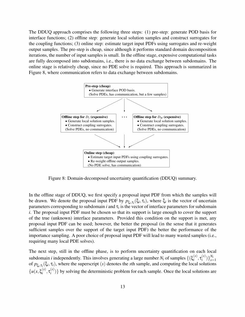
To illustrate the performance of DEIM-CUR as compared to a leverage score algorithm, the fol-lowing example builds a matrix A ∈ R300,000×300 having the form

A =10

∑j=1

1000j

x jyTj +

300

∑j=11

1j

x jyTj , (3)

where x j ∈ R300,000 and y j ∈ R300 are sparse vectors with random nonnegative entries (in MAT-LAB, x j = sprand(30000,1,0.025) and y j = sprand(300,1,0.025)). In this instantiation, about18% of all entries of A are nonzero. The form (3) is not a singular value decomposition, since thevectors in x j and y j are not orthonormal; however, due to the sparsity of these vectors thisdecomposition suggests the structure of the SVD: the singular values decay like 1/ j, and with thefirst ten singular values weighted more heavily to give a significant drop between σ10 and σ11.

Figure 11 compares the error ‖A−CUR‖ of the CUR approximation for DEIM-CUR to two meth-ods based on leverage scores. For the first method, the rank-k approximation takes the k rows andcolumns that have the largest leverage scores computed using only the leading 10 left and rightsingular vectors; the second method is the same, but using all singular vectors. Both methods per-form rather more poorly than DEIM-CUR, which closely tracks the optimal value σk+1. As seenin Figure 11, the DEIM-CUR approach delivers an excellent approximation, while selecting therows and columns with the leading leverage scores does not perform nearly as well.

Figure 11: Accuracy of CUR approximations using k columns and rows, for DEIM-CUR andtwo leverage score strategies for the sparse, nonnegative matrix (3). “LS(all)” selects rows andcolumns having the highest leverage scores computed using all 300 singular vectors; “LS(10)”uses the leading 10 singular vectors.

17

Acknowledgment/Disclaimer

This work was sponsored (in part) by the Air Force Office of Scientific Research, USAF, undergrants/contract numbers FA9550-12-1-0155, FA9550-12-1-0420. The views and conclusions con-tained herein are those of the authors and should not be interpreted as necessarily representing theofficial policies or endorsements, either expressed or implied, of the Air Force Office of ScientificResearch or the U.S. Government.

References

[1] H. Antil, S. Hardesty, and M. Heinkenschloss, Shape Optimization of Shell Structure Acous-tics, Technical Report, Department of Computational and Applied Mathematics, Rice Uni-versity, 2014. Submitted (in review).

[2] H. Antil, M. Heinkenschloss, and D. C. Sorensen, Application of the Discrete EmpiricalInterpolation Method to Reduced Order Modeling of Nonlinear and Parametric Systems. In:Reduced Order Methods for Modeling and Computational Reduction, A. Quarteroni and G.Rozza (eds.). MS&A. Model. Simul. Appl., Vol. 9, 2014, pp. 101-136, Springer Verlag. doi:10.1007/978-3-319-02090-7 4

[3] M. Bambach, M. Heinkenschloss, and M. Herty, A Method for Model Identification and Pa-rameter Estimation. Inverse Problems, 2013, Vol. 29, No. 2, pp. 025009, doi:10.1088/0266-5611/29/2/025009.

[4] P. Benner, M. Heinkenschloss, J. Saak, and H. K. Weichelt, Inexact low-rank Newton-ADI method for large-scale algebraic Riccati equations. Max Planck Institute Magde-burg, Germany,Technical Report MPIMD/15-06, May 2015. Available at http://www.mpi-magdeburg.mpg.de/preprints.

[5] R. Carden and D.C. Sorensen, Automating DEIM for Nonlinear Model Reduction. TechnicalReport CAAM TR12-16, available on line at http://www.caam.rice.edu/tech reports.html,

[6] J. W. Gohlke, Reduced Order Modeling for Optimization of Large Scale Dynamical Systems,Masters Thesis, Department of Computational and Applied Mathematics, Rice University,2013.

[7] D. P. Kouri, M. Heinkenschloss, D. Ridzal, and B. G. van Bloemen Waanders A Trust-Region Algorithm with Adaptive Stochastic Collocation for PDE Optimization under Un-certainty. SIAM Journal on Scientific Computing, 2013, Vol. 35, No. 4, pp. A1847-A1879,doi: 10.1137/120892362.

[8] D. P. Kouri, M. Heinkenschloss, D. Ridzal, and B. G. van Bloemen Waanders Inexact Objec-tive Function Evaluations in a Trust-Region Algorithm for PDE-Constrained Optimization

18

under Uncertainty. SIAM Journal on Scientific Computing, 2014, Vol. 36, No. 6, pp. A3011-A3029, doi: 10.1137/140955665.

[9] Q. Liao and K. Willcox, A Domain Decomposition Approach for Uncertainty Analysis,SIAM Journal on Scientific Computing, 2015, Vol. 37, No. 1, pp. A103–A133, doi:10.1137/140980508.

[10] B. Peherstorfer, D. Butnaru, K. Willcox and H.-J. Bungartz, Localized Discrete Empirical In-terpolation Method, SIAM Journal on Scientific Computing, 2014, Vol. 36, No. 1, pp. A168–A192, doi: 10.1137/130924408.

[11] D.C. Sorensen and M. Embree, A DEIM Induced CUR Factorization CAAM Technical Re-port TR14-04, (2014).

[12] T. Takhtaganov, High-Dimensional Integration for Optimization Under Uncertainty, MastersThesis, Department of Computational and Applied Mathematics, Rice University, 2015.

[13] D. Wirtz, D.C. Sorensen and B. Haasdonk, A-posteriori Error Estimation for DEIM ReducedNonlinear Dynamical Systems, SIAM Journal on Scientific Computing, 2014, Vol. 36, No. 2,pp. A311–A338, doi: 10.1137/120899042.

19

Response ID:4753 Data

1.

1. Report Type

Final Report

Primary Contact E-mailContact email if there is a problem with the report.

heinken@rice.edu

Primary Contact Phone NumberContact phone number if there is a problem with the report

713-348-5176

Organization / Institution name

Rice University

Grant/Contract TitleThe full title of the funded effort.

COLLABORATIVE RESEARCH: MODEL REDUCTION FOR NONLINEAR AND PARAMETRIC SYSTEMSWITH UNCERTAINTY

Grant/Contract NumberAFOSR assigned control number. It must begin with "FA9550" or "F49620" or "FA2386".

FA9550-12-1-0155

Principal Investigator NameThe full name of the principal investigator on the grant or contract.

Heinkenschloss, Matthias

Program ManagerThe AFOSR Program Manager currently assigned to the award

Dr. Fariba Fahroo, Dr. Jean-Luc Cambier

Reporting Period Start Date

04/15/2012

Reporting Period End Date

04/14/2015

Abstract

This project has developed and analyzed new mathematical algorithms to substantially reduce thecomplexity of simulating and optimizing parametrically dependent systems and to support decision-makingunder uncertainty. Specifically, this research has advanced the state of the art in reduced order modelingbased on projections and on the discrete empirical interpolation method (DEIM) for nonlinear systems,developed new adaptive sampling methods for optimization of systems with uncertain inputs, devised adomain decomposition based methods to systematically integrate the uncertainty propagation throughcomponents into uncertainty propagation through a systems composed of these components, established aso-called CUR factorization based on the DEIM that provides a low rank approximate factorization of agiven large matrix with applications to POD model reduction and analysis of data. The feasibility of ouralgorithms was demonstrated on a number of problems with relevance to the Air Force.

Distribution StatementThis is block 12 on the SF298 form.

Distribution A - Approved for Public Release

Explanation for Distribution Statement

If this is not approved for public release, please provide a short explanation. E.g., contains proprietary information.

SF298 FormPlease attach your SF298 form. A blank SF298 can be found here. Please do not password protect or secure the PDF

The maximum file size for an SF298 is 50MB.

SF298_Form_Rice_July10_2015.pdf

Upload the Report Document. File must be a PDF. Please do not password protect or secure the PDF . Themaximum file size for the Report Document is 50MB.

FinalReport2015.pdf

Upload a Report Document, if any. The maximum file size for the Report Document is 50MB.

Archival Publications (published) during reporting period:

See attached report

Changes in research objectives (if any):

None

Change in AFOSR Program Manager, if any:

None

Extensions granted or milestones slipped, if any:

None

AFOSR LRIR Number

LRIR Title

Reporting Period

Laboratory Task Manager

Program Officer

Research Objectives

Technical Summary

Funding Summary by Cost Category (by FY, $K)

Starting FY FY+1 FY+2

Salary

Equipment/Facilities

Supplies

Total

Report Document

Report Document - Text Analysis

Report Document - Text Analysis

Appendix Documents

2. Thank You

E-mail user

Jul 12, 2015 17:52:55 Success: Email Sent to: heinken@rice.edu